Download HF Modulation Analysis

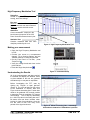
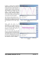
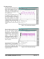
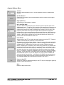
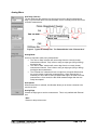
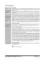
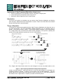
For the SIA-3000
Applications of High Frequency Modulation Analysis tool
•
•
•
View accumulated jitter in the modulation domain—the signal causing the jitter.
Look at the frequency components of jitter using an FFT.
View how the jitter changes over time or output cycles.
Introduction
The focus of this guide is to familiarize the user with the High Frequency Modulation tool allowing
quick and easy measurements and interpretation of results. Refer to the SIA-3000 User’s Manual
and the VISI help files for more information.
Theory of Operation
The analysis of measurements gathered with the High Frequency Modulation tool allows the user to
see jitter accumulation. This tool automatically creates histograms over an increasing range of
periods. The process is shown in Figure 1. The SIA-3000 builds a histogram of time measurements
for a single period, then increments and makes another histogram of two periods, repeating this
process until enough periods are spanned to cover the –3dB frequency.
The 1-Sigma and Peak-to-Peak values from each histogram can then be plotted relative to the
Figure 1. High Frequency Modulation Analysis data acquisition
number of periods spanned. These plots allow you to see how jitter changes or accumulates over
increasing numbers of periods. In doing so, we are able to see the Jitter Modulation. This time
domain data can be transformed to the frequency domain by using an FFT of the autocorrelation of
the variance of the 1-sigma values. Frequency vs. power can then be plotted.
HIGH FREQUENCY MODULATION ANALYSIS
©WAVECREST Corporation 2002
Page 1 of 12
200015-01
REV A
High Frequency Modulation Tool
Dialog Bar
Access to Acquire, FFT algorithm,
Arming, and Filter settings.
Plot area
Zoom in—hold down left mouse button,
expand zoom box over area of interest.
Zoom out—double click left mouse.
Status Bar
Cursor coordinates - Displayed in the
box at lower right portion of the VISI
Panel. Units are same as those in plot.
Statistics View
Contains measured data from each
view/plot provided by the tool.
Figure 2. High Frequency Modulation Tool
Making your measurement
• Open the High Frequency Modulation tool
in VISI.
• Connect your source to a measurement
channel. Go to “Acquire Options” and use
“Add/Del Channel” to select that channel.
• On the Front Panel or Tool Bar, press
“Pulse Find” .
• Verify the voltage levels and close out the
pulse find box.
• Press the Single Acquire button .
Understanding the Results
Figure 3. Instrument Setup
All of the measurements and data required
to calculate and display the different views
or plots available in the tool are gathered
simultaneously on one pass or acquisition.
Before investigating the FFT, start by
viewing the 1-Sigma vs span plot/view
(Figure 4). Try to get at least two full cycles
of the modulation of interest. Note that
Figure 4 shows increasing jitter. Further data
needs to be gathered over enough periods
to determine if this is modulation or if it stops
accumulating. This is done by decreasing
the –3db Freq value in the Dialog bar menu.
Be aware that test times increase when
looking for lower freq modulation, since the
tool will need to look over many more
periods of the signal under test.
HIGH FREQUENCY MODULATION ANALYSIS
©WAVECREST Corporation 2002
Figure 4. Shows increasing jitter—not enough
information to determine if modulation is present.
Page 2 of 12
In Figure 5, –3db Freq value on the Dialog
Bar has been decreased to 15.0 KHz (from
100KHz in figure 4). The periodic nature of
the plot data clearly shows that there is
modulation present. The jitter increases to a
maximum of about 851ps over 370 Periods
and decreases to a minimum over 748
periods. The minimum 1-sigma values are
constant. A lower frequency modulation
would be indicated if the minimum 1-Sigma
values were increasing. A further reduction
in the –3db Freq value would measure over
more periods to show this modulation.
After viewing the data provided by the 1sigma vs span view (Figures 4 & 5), use the
keyboard Page up or Page down keys to see
the frequency and amplitude of the periodic
jitter components in the FFT views (Figure
6).
Figure 5. Shows the jitter modulation over more
periods.
These
views
are
FFT’s
of
the
autocorrelation, of the variance of the 1sigma values in the 1-sigma vs span plot.
Two FFT views are provided: FFT N-clk and
1-clk. The N-clk view shows every jitter
frequency as having equal effects on a
period of the carrier frequency.
The 1-clk view shows how the jitter
frequency components and amplitude affect
a single clock period. Low Frequency jitter
has a smaller effect on the jitter of a single
clock period. Compared to the N-clk view,
the 1-clk view has a 20 db/decade roll-off for
low frequencies. Therefore, Low frequency
jitter components are lower in amplitude.
Figure 6. Shows the N-clk FFT. A 1MHz peak is
present.
HIGH FREQUENCY MODULATION ANALYSIS
©WAVECREST Corporation 2002
Page 3 of 12
PLL Measurements
This section covers the measurement of
Phase Locked Loop (PLL) devices using
this tool. When analyzing PLL’s, the 1Sigma Plot responses produce a
characteristic curve, which indicates the
noise response and bandwidth of the
PLL’s feedback loop.
Figure 7 shows the analysis of a PLL. In
the displayed 1-Sigma vs Span view;
note the characteristic loop response of
the PLL over ‘N’ periods. The 1-sigma
jitter values increase over a small
number of periods (x-axis). This relates
to high frequencies. At a certain number
of periods (or frequency) the jitter stops
accumulating, and the jitter (or
modulation) effects are seen as hills and
valleys.
Figure 7. PLL response with modulation
Also, note that any rising curve that
settles at a high level will be seen by an
FFT as a low frequency component
(see Figure 8). The FFT treats the
rising curve as the first part of an entire
modulation curve. The FFT will show
a very low frequency spike, which is an
artifact.
Any
real
frequency
components will remain constant in
frequency and amplitude as –3db Freq
is decreased to view more cycles of
the clock, but any artifact will move
down in frequency.
Figure 8 shows the FFT of the 1-sigma
data from Figure 7. The low frequency
shoulder is an artifact caused by the
rising curve of the 1-Sigma plot. Notice
that the frequency spike to the right of
the artifact is the true deterministic jitter
component at 1MHz.
HIGH FREQUENCY MODULATION ANALYSIS
©WAVECREST Corporation 2002
Figure 8. The FFT of the data from Fig 8.
Page 4 of 12
High Frequency Modulation Main Menu
View
The View pull-down menu provides the user several different ways to see the
acquired measurement data, depending on the active tool.
Acquire Options
Opens the Acquire Options menu.
Arming
Opens the Arming menu.
Voltages
Opens the Voltages menu.
RJ+PJ Filters
Opens the RJ+PJ Filters menu.
View Options
Opens the View Options menu.
HIGH FREQUENCY MODULATION ANALYSIS
©WAVECREST Corporation 2002
Page 5 of 12
Acquire Options Menu
Channel
Opens the channel selection menu. Use the keypad to select one measurement
channel.
Hits Per Measure
Determines the number of time measurements that will be made for each edge or
point on the plot.
Edge to Measure
Select Rising or Falling edge to measure.
HPF –3dB Freq (kHz)
The HPF -3dB low rolloff frequency is the frequency of the half power point of the
20dB/decade “knee”. The choice of this frequency will determine the low frequencies
visible on the FFT. The -3dB Frequency (kHz) is used to determine the maximum
measurement interval to be used in sampling and is entered in kHz. A lower -3dB
Frequency extends the time required to acquire the measurement set because
histograms over many more periods must be acquired. Below the -3dB Frequency, a
natural roll-off of approximately 20dB per decade is observed. The default value is
100kHz. -3dB Frequency affects how much data is acquired and, therefore, the
choice of this value also affects the test time.
Fmax Divider
Allows scaling of the FFT by dividing the upper frequency end of the FFT. Default is
1 which shows frequencies of jitter up to 1/2 the clock rate.
Changing this value allows faster analysis of lower frequency information by skipping
edges and ignoring high frequency effects. However, changing this value without
changing the HPF -3dB frequency will reduce the number of edges measured.
NOTE: Depending on the frequency of the clock being measured, it is possible that
the Nyquist of the clock (1/2 the clock rate) could intrude into or is below the region
chosen as the First Order filter frequency. Additionally, if the Fmax Divider is set at
any value other than one, this will eliminate any frequency content above divided
Fmax. For example, if measuring a 400MHz clock, the Fmax or Nyquist is 200MHz.
Therefore, a First Order filter set to 20MHz would be 20dB down at 200MHz. But, if
the Fmax divider is set to '2', then the "Nyquist" or "Fmax" would be 100MHz and
would cut into the first order filter. In this case, the RJ (RMS) value measured may
not contain the same spectral content as did the measurement with Fmax set to '1'.
The reported RJ(RMS) value would be lower with the Fmax set to '2'.
Passes to Avg FFT
Selects the number of passes to average for the FFT output. Averaging will generally
reduce the noise floor of the FFT.
Back
Returns to the previous menu.
HIGH FREQUENCY MODULATION ANALYSIS
©WAVECREST Corporation 2002
Page 6 of 12
Arming Menu
Arm Delay (19-21ns)
The arm delay sets the minimum time from an arm event to the first measurement
edge. Figure 3 shows there is a user selectable 19 to 21 ns delay from the Arm event
to the first measurement.
Figure 3. Typical Arm Setup time. The Pattern Marker is the “External Arm”
Arming Mode
An arm is required to make every measurement.
• The “Arm on Stop” selection will use an edge from the currently chosen
measurement channel. 'Stop' refers to using an edge type (rising or falling)
that begins the.
• The “Arm on Start” selection will use an edge from the currently chosen
measurement channel. 'Start' refers to using an edge type (rising or falling)
that begins the measurement.
• The “External Arm” selection will use an edge from a channel different than
the one(s) chosen to make the measurement(s). When 'External Arm' is
selected, you will be able to select a channel and edge to be used to arm the
measurement. Once armed, the SIA-3000 measures edges after the Arm
Delay has elapsed.
Arm Number
When External Arm is selected, Arm Number allows you to choose a channel to be
used as the Arm.
Arming Edge
Choose the edge type to arm the measurement. This is only available with External
Arm.
Back
Returns to the previous menu.
HIGH FREQUENCY MODULATION ANALYSIS
©WAVECREST Corporation 2002
Page 7 of 12
Voltages Menu
Threshold Voltage
When set to AUTO, sets start and stop threshold reference voltages based on the
minimum and maximum level found on each channel (from Pulsefind).
The
threshold is automatically set to the 50% point. The voltages are shown in the
voltage display boxes after a pulsefind is completed.
Select "USER VOLTS" to manually enter threshold voltages in the voltage display
boxes. A pulsefind cannot be performed with this setting.
Channel Voltage
When "Threshold Voltage" is set to AUTO, use the "channel" control to view the
threshold voltages derived from PULSEFIND. Voltages are displayed under
“Channel Voltage". In USER VOLTS, the voltage can be set here.
Arm Voltage
When "Threshold Voltage" is set to AUTO, use the "channel" control to view the
threshold voltages derived from PULSEFIND. Voltages are displayed under "Arm
Voltage". In USER VOLTS, the voltage can be set here.
Back
Returns to the previous menu
HIGH FREQUENCY MODULATION ANALYSIS
©WAVECREST Corporation 2002
Page 8 of 12
RJ+PJ Filters Menu
RJ+PJ HPF
Natural Rolloff – Uses the –3dB frequency as the “Natural Rolloff”. This is a “Natural
Rolloff” because the amount of data acquired by the tool naturally limits the lowest
frequency "seen".
Brickwall – Brick wall cuts off any frequencies below this value. Note that the –3dB
frequency should be lower than the brick wall cutoff or the natural rolloff will have a
filtering effect.
NOTE: Depending on the frequency of the clock being measured, it is possible that
the Nyquist Frequency of the clock (1/2 the clock rate) could intrude into or be below
the region chosen as the First Order filter frequency. Additionally, if the Fmax Divider
is set at any value other than one, this will eliminate any frequency content above
divided Fmax. For example, if measuring a 400MHz clock, the Fmax or Nyquist is
200MHz. Therefore, a First Order filter set to 20MHz would be 20dB down at
200MHz. But, if the Fmax divider is set to '2', then the "nyquist" or "Fmax" would be
100MHz and would cut into the first order filter. In this case, the RJ(RMS) value
measured may not contain the same spectral content as did the measurement with
Fmax set to '1'. The reported RJ(RMS) value would be lower with the Fmax set to '2'.
High Pass Freq (MHz)
Lower frequency limit for the window over which RJ and PJ is calculated. Default is
Corner Frequency. This setting cannot be set lower than the corner frequency.
RJ+PJ Low Pass Filter (LPF)
Nyquist – This is the default. The highest frequency that the tool can measure is ½
the clock rate (or the Nyquist).
First Order – Enter a -3dB frequency. This filter does not eliminate all the jitter
energy above this frequency (it is not a brick wall filter). The frequency components
or spectral content above this frequency will still contribute to the RJ(RMS) as
displayed from the 1-sigma plot. (see figure)
NOTE: Depending on the frequency of the clock being measured, it is possible that
the Nyquist of the clock (1/2 the clock rate) could intrude into or be below the region
chosen as the First Order filter frequency. Additionally, if the “Fmax Divider” is set at
any value other than one, this will eliminate any frequency content above divided
Fmax. For example, if measuring a 400MHz clock, the Fmax or Nyquist is 200MHz.
Therefore, a First Order filter set to 20MHz would be 20dB down at 200MHz. But, if
the “Fmax Divider” is set to '2', then the Nyquist or Fmax would be 100MHz and
would cut into the first order filter. In this case, the RJ(RMS) value measured may
not contain the same spectral content as did the measurement with Fmax set to '1'.
The reported RJ(RMS) value would be lower with the Fmax set to '2'.
Low Pass Freq (MHz)
Upper frequency limit for the window over which RJ and PJ is calculated. Default is
the Nyquist frequency.
Back
Returns to the previous menu
HIGH FREQUENCY MODULATION ANALYSIS
©WAVECREST Corporation 2002
Page 9 of 12
View Options Menu
FFT Window
To reduce spectral information distortion of FFTs, the time domain signal is multiplied
by a window weighting function before the transform is performed. The choice of
window will determine which spectral components will be isolated, or separated, from
the dominant frequency(s). Each window function has advantages/disadvantages
over other windows.
FFT, Padding Multiplier
Padding increases the frequency resolution of the FFT. Generally, a higher padding
value will increase transformation processing time.
FFT Alpha Factor
Varying the Alpha Factor illustrates the inverse proportionality relationship between
the spectral peak width and the sidelobe rejection of the Kaiser-Bessel window. As
the Alpha Factor increases, the spectral peak widens and the side lobes shrink. As
the Alpha Factor decreases, the spectral peak narrows and the side lobes increase in
amplitude.
X-axis
Select the horizontal plot axis unit of measure.
Delay Time - Shows time from Arm
Delay Periods - Shows number of periods from Arm
Elapsed Time - Shows elapsed acquisition time
Event - Take a measurement for each event from START event to STOP event and
plot these values versus the count.
Hit Number - Low Frequency Modulation: Hit number is integer value assigned to
each measurement as it is made.
Measurement - Shows number of total measurements
Span Periods - Shows number of periods measured
Span Time - Shows units of time measured
Time - Take a measurement and plot the value versus time.
UI Spans - Shows number of UI spans measured
Back
Returns to the previous menu
HIGH FREQUENCY MODULATION ANALYSIS
©WAVECREST Corporation 2002
Page 10 of 12
Summary
The High Frequency Modulation Analysis tool capitalizes on the capabilities of the SIA-3000’s internal
architecture, specifically, the Nth event counters. The ability of the counters to span multiple edges or
periods allows the SIA-3000 to perform measurements allowing it to view jitter modulation of the signal
under test. This data is plotted on either a 1-sigma vs span view or an FFT view. Performing an FFT of
the autocorrelation of the variance from the 1-sigma information will give a frequency vs power plot
allowing the user to see the frequency components of the jitter modulation and their respective
amplitudes.
HIGH FREQUENCY MODULATION ANALYSIS
©WAVECREST Corporation 2002
Page 11 of 12
For more information contact:
WAVECREST Corporation
7626 Golden Triangle Dr
Eden Prairie, MN 55344
www.wavecrest.com
1(952)-646-0111
HIGH FREQUENCY MODULATION ANALYSIS
©WAVECREST Corporation 2002
Rev09.11.02_tag
Page 12 of 12
200015-01
REV A