Download Quick Start Guide

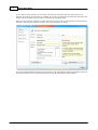
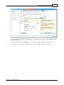
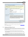
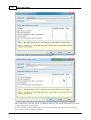
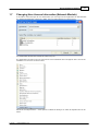
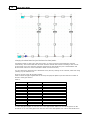
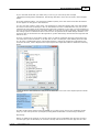
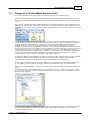
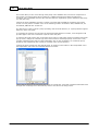
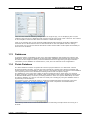
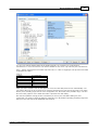
Piping Systems FluidFlow
Quick Start
Owned and Copyright by Flite Software NI Ltd
I
Quick Start Guide
Table of Contents
Foreword
Part I Piping Systems FluidFlow
0
1
1 Welcome
................................................................................................................................... 1
2 Installation
................................................................................................................................... 1
3 Activation
................................................................................................................................... 1
4 Keeping
...................................................................................................................................
your Software Current
5
5 Network
...................................................................................................................................
Issues
6
6 Starting
...................................................................................................................................
the Application (Network Module)
9
7 Changing
...................................................................................................................................
User Access Information (Network Module)
11
8 Application
...................................................................................................................................
Layout
13
9 Design
...................................................................................................................................
of a cooling water system
14
10 Design
...................................................................................................................................
of a Tank Farm Gas Collection System
27
11 Design
...................................................................................................................................
of a Cooling Water System. Part 2.
29
12 Configuration
...................................................................................................................................
and Environment
32
13 Databases
................................................................................................................................... 33
14 Fluids
...................................................................................................................................
Database
33
15 Database
...................................................................................................................................
of Manually Operated Valves
35
16 Add
...................................................................................................................................
a New Pump
38
Index
40
Flite Software NI Ltd
Piping Systems FluidFlow
1
Piping Systems FluidFlow
1.1
Welcome
1
Welcome to Piping Systems FluidFlow a state-of-the-art fluid flow simulator. This software application
allows you to simulate the flow of fluids in complex networks, taking into account the phase state of
the fluid and determining heat changes. FluidFlow is more than a pipe network analysis program, it is
a fully developed steady-state process-flow simulator.
System Requirements
1024 MB RAM (2048 MB recommended)
Microsoft Windows Server 2008, 2003, Windows 7, Windows 8, Vista or XP
80MB of free hard disk space
SVGA or higher resolution monitor (XGA recommended)
Mouse or other pointing device
1.2
Installation
FluidFlow is supplied as a single compressed installation file - FF3SETUP.EXE. This file is available via
a download from our website www.fluidflowinfo.com (preferred method).
This is a common installation file for all possible modules. Simply run the file FF3SETUP.EXE and the
installer will start and take you through the setup process. You can also use the setup program to
install updates into your installation folder (only executable, help files etc are updated, databases
and your project files are not overwritten).
It is possible to install remotely if you are a network administrator. The installation does not require
any registry entries and for users not wishing to use an installer (for example in locked
environments) there is a zipped version of the application and associated folders.
This product has been fully tested and can also be installed to run under C itrix or Terminal Services.
If you intend to run many concurrent users across remote locations outside of a LAN, (i.e. a WAN
across country borders) you need to purchase a global licence.
Once installed the software reverts to demo mode until it is activated. So the first thing you need to
do after installation is to Activate the software. There is a simple activation process for both installed
and unzipped installations.
In order to activate and run the software you MUST have read/write access to the folder where
FluidFlow is installed. You cannot activate over a LAN or WAN without using terminal services, remote
desktop, citrix etc, since for activation the application MUST be running in the server process
workspace. For more information about the activation process see the activation chapter.
1.3
Activation
Activation is the process of configuring access to the available FluidFlow modules. After a new
installation there are no active modules.
From FluidFlow V3.3, the product activation can be carried out automatically. When FluidFlow is
started for the first time the following dialog appears
© <2013> ... Flite Software NI Ltd
2
Quick Start Guide
If you wish to defer activation or do not have an internet connection then press No and you can
activate via email or directly from our website. If you have an internet connection then select the Yes
button and the activation process will be completed as described below.
When you purchase the software or obtain a demo licence you will be provided with a Username and
Password. Use the information provided in the Licence Manager as shown.
Press the Activate FluidFlow3 button and the software will automatically obtain an activation code and
activate the software. If a successful activation occurs the following message appears
© <2013> ... Flite Software NI Ltd
Piping Systems FluidFlow
3
All of the alternative activation methods that were available prior to V3.3 are still available and these
are described below.
You can use the 'Help | Activate FluidFlow...' menu option, which will display the dialog below.
C lick on the "How to Register" tab and select one of the available registration methods.
© <2013> ... Flite Software NI Ltd
4
Quick Start Guide
The software generates a Product Id (9DFC -D803 in the example above) directly from your
computer. Simply email this Product Id together with the calculation modules you need, or have
purchased, to [email protected] and an activation code and registration name will be
provided (usually by return).
On receipt of your activation code and registration name (you can specify the registration name if
you wish in the email you send to us), click on the "Activate" tab and enter the information you have
received as shown below.
Assuming we have received the following activation data:
Registration Name: Flite Software NI Ltd
Activation C ode:
0A0306A5365AAF07A3F28D3FA20BFB5C7BE5682AB8571C880EBF57FD384AB966A91D7A987EE0338F7EDFBF57FD384AB966A922ADEA59EF25E4
187DBF57FD384AB966A9A3BFF345B0BA0CEACBAF6A2F9111094829563E472CE22F9180EFAF6A2F911109482940AF7E349247A69F8BF57FD384A
B966A932CCEDCABF38D8FF4AF6A2F9111094829DBAEB3D1623F8B8BFAF6A2F9111094829256BDC8D142CD1ED6AF6A2F911109482918FF7329
00F4D7F42AF6A2F91110948291
C opy and paste this information from your email.
© <2013> ... Flite Software NI Ltd
Piping Systems FluidFlow
5
Press the 'Activate FluidFlow' button and the Registration Id will now contain a code instead of
Evaluation Version and the modules that you have purchased will become available.
Once activated you should quit the application and restart. This step is important for correct
activation.
If you are activating a network version then you should also read the network activation and setup
section for additional information.
1.4
Keeping your Software Current
Flite Software has a commitment to constant improvement of the FluidFlow product. In addition we
provide an undertaking to attempt to fix bugs and annoyances in a timely manner. This commitment
means that the FluidFlow product is constantly improving and so it is in your interest to stay current
by using the latest release.
From Version 3 we have adopted the following numbering convention for product versions.
All minor bug fixes for a given version will be implemented via new builds of the same version.
This is in contrast to the old system used for V2 product, which always incremented the version
number for all bug fixes.
Only enhancements or new features will cause a version number increment to occur. For example,
in the past any new bugs reported for version 2.26 would be fixed and appear in a 2.27 version
only. Now, any new bugs reported for version 3.15 Build 1 will be fixed and will appear in version
© <2013> ... Flite Software NI Ltd
6
Quick Start Guide
3.15 Build 2. Written as 3.15.2
All version numbers have the format [Major Version].[Minor Version] Build Number, for example,
3.22 Build 5 means a Version 3 product with a Minor Version number of 22 and a Build Number of
5. Written as 3.22.5
It is your responsibility to keep your software current via our website. We have a Software
Assurance Policy that enables continued access to the downloads area of our website:
http://www.fluidflowinfo.com/Downloads/Downloads.asp
1.5
Network Issues
Note: This section is only relevant if you have the Network module.
Network Installation
The installation process on the network is the same as stand-alone: simply run FF3SETUP.EXE.
FluidFlow can be installed across a network as long as you use terminal services, remote desktop, or
a similar access method. The network folder MUST have write access, which usually means you must
have admin rights during the installation process. FluidFlow does not use or require access to the
Registry.
After installation your network users must be given permission/access rights to the FluidFlow folder.
We would suggest that users are given full access to the folder that FluidFlow is installed in, e.g.,
\Flite\FluidFlow3, and that this access is propagated through the sub-folders.
However, if you wish to restrict full access, FluidFlow requires read access to all folders, and
additionally, write access to the following folders:
\Flite\FluidFlow3
\Flite\FluidFlow3\Data (and all sub-folders)
\Flite\FluidFlow3\Preferences (and all sub-folders)
Note: In Windows XP, it is not enough to just change the properties of the folder(s), you must also
check the 'Allow network users to change my files' checkbox in the Network Sharing and Security
Properties for the folder. (Note: This can be accessed in Windows Explorer via the Properties context
menu item, then the Sharing tab.)
Overriding the location of the Read-Write Folders
With some network installations, Administrators prefer to have control over which folders client users
have read-write access to. To cater for this, FluidFlow provides PSFF.INI which allows the
Administrator to specify the default location for \Data, \Preferences, and the Network Access files.
Note: FluidFlow does not create this INI file itself; it is the responsibility of the Network Administrator
to create PSFF.INI and place it in the same folder as PSFF.EXE. If you wish to use a psff.ini file follow
the explanations below;
PSFF.INI
[Options]
; Data
UseCommonAppDataFolder=0
DataFolder=
; Preferences
UseLocalAppDataPreferencesFolder=0
PreferencesFolder=
; Network Access
UseCommonAppDataNetworkAccessFolder=0
NetworkAccessFolder=
Data
If UseC ommonAppDataFolder=1 then FluidFlow will use the "C :\Document and Settings\All
© <2013> ... Flite Software NI Ltd
Piping Systems FluidFlow
7
Users\Application Data\FluidFlow3\Data" folder. Otherwise FluidFlow will use the value of the
DataFolder entry. If this is blank, or PSFF.INI does not exist, then FluidFlow will use "\FluidFlow3
\Data".
NOTE: If DataFolder is specified then this folder MUST exist.
Preferences
If UseLocalAppDataPreferencesFolder=1 then FluidFlow will use the "C :\Document and
Settings\[Username]\Local Settings\Application Data\FluidFlow3\Preferences" folder. Otherwise
FluidFlow will use the value of the PreferencesFolder entry + [Username]. If this is blank, or PSFF.INI
does not exist, then FluidFlow will use "\FluidFlow3\Preferences\[Username]". [Username] is the
windows log on name of the user.
Network Access
If UseC ommonAppDataNetworkAccessFolder=1 then FluidFlow will use the "C :\Document and
Settings\All Users\Application Data\FluidFlow3" folder. Otherwise FluidFlow will use the value of the
NetworkAccessFolder entry. If this is blank, or PSFF.INI does not exist, then FluidFlow will use
"\FluidFlow3".
NOTE: If NetworkAccessFolder is specified then this folder MUST exist.
Network Activation
Although FluidFlow can be installed across a network, it must be activated from the installation on
the server machine. This means you must be either physically at the server or accessing the server
remotely via terminal services, citrix etc. You cannot activate the server via normal LAN access.
When contacting Flite for an Activation C ode, please state how many users the network license is
for.
To contact Flite and receive your Activation C ode:
Ring Flite on Int+44 2871 279227. You will need to quote your Product Id, specify a Registration
Name, and the Modules you require.
E-mail [email protected]. You will need to include your Product Id, a Registration Name, and
the Modules you require.
When you enter the Activation C ode you will need to restart FluidFlow for it to take effect.
Client Setup
After installing and activating FluidFlow on the network server you can set up the client machine by
placing a link on the client's desktop to FluidFlow. To do this, assuming that FluidFlow3 is the name of
the shared folder:
1. Right-click on the desktop and select the 'New | Shortcut' menu item.
2. Type the location of the PSFF.EXE file, e.g., '\\Server\FluidFlow3\PSFF.exe' and click 'Next'.
3. Enter the title for the shortcut, e.g., 'FluidFlow3 (Network)' and click 'Finish'.
Note: If you do place a link on the desktop to FluidFlow on the network server, then this may affect
the startup speed of the client machine. This is because on startup the client will search the Network
Neighbourhood to find the link's target. Normally, if the network server is always on, this will take no
noticeable time; however, if the network server is down, you may notice some small extra delay in
startup. (Note: This is not specific to FluidFlow, but is true of all applications linked to a network
resource.)
Help Files on the Network
From FluidFlow release V3.22.4 help files work across a LAN or WAN automatically.
If you are not using the current production release then the following info may be important in order
© <2013> ... Flite Software NI Ltd
8
Quick Start Guide
to get your help files operating over a network.
R e c e nt s e c urity up d a te s to W ind o w s X P ha v e intro d uc e d s o m e s e v e re re s tric tio ns fo r a c c e s s ing HT M L
He lp file s a c ro s s ne tw o rk d riv e s . U nd e r W ind o w s X P a nd V is ta m o s t file link s in HT M L He lp file s w ill
no w g e ne ra lly no t w o rk a t a ll a nd HT M L He lp its e lf is a ls o s e v e re ly re s tric te d . W itho ut re g is try
c ha ng e s o n the us e r's c o m p ute r HT M L He lp no w c a nno t b e us e d a t a ll o n ne tw o rk s . T his ha s a n e ffe c t
o n the Fluid Flo w Ne tw o rk V e rs io n a s a ll c lie nt m a c hine s tha t try to d is p la y the He lp file w ill re c e iv e a
"P a g e no t fo und " m e s s a g e .
M o re d e ta ils a nd a fix fo r this p ro b le m a re a v a ila b le o n the He lp & M a nua l w e b s ite .
A lte rna tiv e ly , the re is a w o rk a ro und to a llo w a c lie nt m a c hine to d is p la y Ne tw o rk -b a s e d HT M L He lp
file s , b ut it d o e s inv o lv e m o d ify ing the R e g is try o n the c lie nt m a c hine . T o d o this :
1. C lic k 'Sta rt', c lic k 'R un', ty p e 're g e d it', a nd the n c lic k 'O K '.
2. Lo c a te a nd the n c lic k the fo llo w ing s ub k e y :
HK EY _LO C A L_M A C HINE\SO FT W A R E\M ic ro s o ft\HT M LHe lp \1.x \Its s R e s tric tio ns
No te : If this re g is try s ub k e y d o e s no t e x is t, c re a te it. T o d o this , fo llo w the s e s te p s :
a . O n the 'Ed it' m e nu, p o int to 'Ne w ', a nd the n c lic k 'K e y '.
b . T y p e 'Its s R e s tric tio ns ', a nd the n p re s s 'ENT ER '.
4. R ig ht-c lic k the Its s R e s tric tio ns s ub k e y , p o int to 'Ne w ', a nd the n c lic k 'DW O R D V a lue '.
5. T y p e 'M a x A llo w e d Z o ne ', a nd the n p re s s 'ENT ER '.
6. R ig ht-c lic k the M a x A llo w e d Z o ne v a lue , a nd the n c lic k 'M o d ify '.
7. In the V a lue d a ta b o x , ty p e '1', a nd the n c lic k 'O K '.
T his w ill a llo w y o u to a c c e s s C HM file s o n a s ha re d ne tw o rk fo ld e r. Fo r m o re info rm a tio n s e e : http ://
s up p o rt.m ic ro s o ft.c o m /?k b id = 896054
No te : A lw a y s m a k e a b a c k up o f the R e g is try b e fo re m a k ing a ny m o d ific a tio ns s o tha t y o u c a n
'ro llb a c k ' the c ha ng e s if a ny thing g o e s a w ry . T o d o this , run R e g e d it, s e le c t the 'File | Ex p o rt' m e nu
ite m , s e le c t the 'A ll' o p tio n fro m 'Ex p o rt R a ng e ', e nte r a file na m e a nd c lic k 'Sa v e '. Y o u c a n la te r us e
the 'File | Im p o rt' m e nu ite m if y o u w a nt to re v e rt to y o ur o rig ina l R e g is try .
Troubleshooting
The most usual issues reported for network installations and their resolutions are given below...
1. Unable to Activate
This is because you are trying to activate from a client machine. This is not possible because
you are running the application in the client workspace and not the server workspace. For the
purpose of activation ONLY, you can overcome this issue by connecting to the server via remote
desktop (terminal services, citrix etc) or being physically present at the server to activate. So to
activate a network version, run the application via remote desktop, or be physically at the server.
Another possible reason for "unable to activate" is because you do not have the correct
read/write/modify permissions to the folder (and all sub folders) where FluidFlow is installed.
2. "User Limit [1] reached. No more users allowed." message always displayed no matter how many
licenses. This is caused by the incorrect sharing of the FluidFlow folder. For more information see the
Network Installation section above.
© <2013> ... Flite Software NI Ltd
Piping Systems FluidFlow
1.6
9
Starting the Application (Network Module)
If you have the network module activated the product starts slightly differently to the start-up of the
stand-alone version.
If you do not have the network module activated then skip this section.
The first step in the start-up for a network user is a simple logon screen:
Select your username from the list and enter the password given to you by the system
administrator.
Select from the available licenses the calculation functionality you will need. In the above below we
have selected liquid, gas and Two-Phase calculations.
Press the OK button and the application will start up proper.
In the below example the user Administrator will be using 3 modules from a total pool of 5.
© <2013> ... Flite Software NI Ltd
10
Quick Start Guide
The next user to log on will see the following Logon dialog.
Notice that there are now less licence's available as liquid, gas and Two-Phase modules were taken
by Administrator who logged on first.
You can skip to the next section unless you are the administrator and wish to set up a group of
users, delete a user, or change a password.
© <2013> ... Flite Software NI Ltd
Piping Systems FluidFlow
1.7
11
Changing User Access Information (Network Module)
To be able to make changes to user information you must logon to the application as Administrator.
The default administrator password is PSFF. Logon as Administrator as shown below:
You must select at least one module in order to log on.
The application will start in the normal manner but an additional item will appear at the end of the
'Database' menu items as shown below:
Select the 'C onfigure Users...' menu option to obtain the dialog from which all adjustments can be
made.
© <2013> ... Flite Software NI Ltd
12
Quick Start Guide
From this dialog you can add or delete users, change passwords, or just view the current
connections.
It is not possible to delete the Administrator.
© <2013> ... Flite Software NI Ltd
Piping Systems FluidFlow
1.8
13
Application Layout
The application work screen consists of two main windows. The flowsheet window where a schematic
layout of the piping network is developed or built, and the data palette where data input is made,
results and warnings are shown, etc.
You can have as many flowsheets open as desired. From a flowsheet viewpoint the application
behaves similar to Microsoft Word's Multiple Document Interface, that is, you can tile, cascade, and
select a flowsheet from the window menu or by clicking on the caption bar of the window. If you
double-click the caption bar the flowsheet fills the available work area.
The data palette size can be adjusted by dragging the left side of the window border. The data
palette is synchronized to the flowsheet, so if you click on a flowsheet element, the data palette is
refreshed to reflect the current selections(s). This process also works in reverse, for example, if you
click an element warning in the data palette, or a list item, the flowsheet selection updates to reflect
this.
At the top of the work screen are three rows of operators: (1) a set of drop down menus; (2) a
toolbar; (3) the component palette. The component palette consists of a series of tab options. Within
each tab are the equipment item icons or elements that are used to build a fluid network.
A flowsheet toolbar is positioned along the left hand side of the screen. Options here determine how
you access and utilize the flowsheet window.
© <2013> ... Flite Software NI Ltd
14
1.9
Quick Start Guide
Design of a cooling water system
This section is based on a simple example that will illustrate some of the basic concepts you can use
in FluidFlow. The example involves designing a cooling water distribution system to three heat
exchangers.
The topics covered in this example design are:
Flowsheet and model building basics
How to enter data
How to interpret results
How to make changes to the model so that we can obtain a better design
Problem Statement:
It is desired to provide a balanced cooling water flow from a cooling tower to 3 shell and tube heat
exchangers HE1, HE2 and HE3. The size of the heat exchangers has already been determined from
the process requirement and is summarized in the following table.
Table 1
Name
HE1
HE2
HE3
Heat Load in W
200000
250000
170000
Tube length in m
3
3
3
Tube diameter in m Number of tubes
0.012
130
0.012
165
0.012
110
The cooling water is to flow through the tubes and the maximum inlet summer temperature of the
cooling water will be 25°C . The design temperature rise of the cooling water is 10°C . The elevation
of the exchangers above the pump centerline is 3m and the exchangers are approximately 7 m
apart. Each exchanger has 2 tube passes.
We need to design/specify the following items.
Pipe sizes to be used.
The method we will use to balance the flow through each exchanger.
How to make a pump selection.
We need to consider what happens to the exit cooling water temperature of HE2 if the heat load is
increased by 33%.
The completed example can be found in the Examples folder "C ooling Water Distribution. First Design
Iteration", "C ooling Water Distribution. Second Design Iteration" ... through to "C ooling Water
Distribution. Final Design Iteration"
Building the model in the FluidFlow flowsheet:
Before we start building the model, let us consider a moment, the design approach we intend to use.
If you have the autoselection or scripting modules installed you would almost certainly use a
different approach to that taken in this example.
Without these modules we will need to take more of a trial and error approach.
With the design of all systems the initial question we need to answer is where do we start and end
the model i.e. where do we and how do we define the model boundaries. For this design we will start
the model at the cooling tower sump and end the model at the top of the cooling tower. This means
the cooling tower will not be included in this model. Most cooling water systems have a supply header
taking fresh cooling water to each individual exchanger and a collection return header, we will use
this same approach.
Finally, before we start building the model we need to consider the cooling water flow we need to
each exchanger branch. The flow to each exchanger is determined by a heat balance. The heat
transferred to the cooling water will be:
Heat Transferred (W) = mass flow (kg/s) x specific heat capacity (J/kg) x temperature rise (°C )
The specific heat of water at 30° C is approx 4154 J/kg, so from Table 1 we see that the mass flow
needed to HE1 will be 200000 / (4154 x 10) = 4.81 kg/s. Summarizing in Table 2
Table 2
Heat Exchanger Name
Mass Flow in kg/s
© <2013> ... Flite Software NI Ltd
Piping Systems FluidFlow
HE1
HE2
HE3
15
4.81
6.02
4.09
We will start building the model by placing 3 shell and tube exchangers onto the flowsheet. Select the
shell and tube exchanger by clicking on the component palette Heat Exchangers Tab and by selecting
the shell and tube icon.
Drop 3 heat exchangers onto a new flowsheet as shown below:
As we drop each element (or component) onto the flowsheet, default data is associated with the
element. The default data for each element can be seen in the data palette by clicking on the Input
Tab. Often we need to change some value(s) in the default data to meet our needs. For now we will
continue building and come back later to change each individual element as necessary.
The reason we are deferring this task is that there are many group features built into FluidFlow to aid
data editing and setup, which we can use later.
Next we will add the two boundaries.
Inlet Boundary:
For the cooling water inlet boundary we need a boundary that can represent the cooling water sump.
We know that the sump is open to atmosphere and that during normal operation the liquid level in
the sump is 0.5m above the pump centreline.
If we specify the pressure at any boundary then FluidFlow will calculate the flow that will be delivered
to the system. In our design we know the design flow that is needed, because this is determined by
the heat load of the exchangers. Later we will make a pump selection that will provide us with the
correct flow.
Select the known flow boundary by clicking on the component palette Boundaries Tab and by
selecting the known pressure icon. Place the known pressure element on the flowsheet anywhere
below the 3 heat exchangers.
Outlet Boundary:
The collection return line eventually leads back to a cooling tower. At this boundary we know (or it is
a design specified condition) the pressure that we must be above in order for the system to work.
The water pressure necessary at the exit boundary is the sum of the elevation we need to rise to the
top of the cooling tower + any pressure required to overcome the loss in the flow distribution system
feeding the cooling water tower. The elevation of the cooling tower inlet above the pump centerline is
6m and the manufacturer of the cooling tower requires a minimum pressure loss of 30000 Pascals
for the flow distribution to work effectively. We will therefore select a known pressure element for
the exit boundary.
© <2013> ... Flite Software NI Ltd
16
Quick Start Guide
At this point the flowsheet should look something like;.
To add a pump with a known flow (in this case our design flow of 14.92 kg/s), we need to select the
pump element found on the Auto tab. If we select a pump from the boosters tab this will represent a
specific pump and the flow we obtain in the system will be that dictated by the intersection of the
pump and system curves. C hances are that the specific pump selection will be incorrect, so we will
defer the selection of the actual pump model until we have sized the pipes. To do this we use the
pump from the Auto tab and specify the system design flow. The auto pump element will calculate
the head required to deliver our design flow and thus provide us with the information to make the
correct pump model selection.
Place an auto pump on the flowsheet to the right of node 4 (the node representing the cooling tower
sump).
We are ready to start connecting pipes. FluidFlow makes pipe connecting very easy, because there is
no need to include bends. These are added for you as you draw the pipes. We will again defer the
task of editing data values as we connect pipes. Right now we are only concerned with building the
model connectivity.
C lick the pipe tool on the steel pipe icon.
As you move the cursor over the flowsheet the shape changes to a pipe
.
C lick on the known pressure boundary and then move the mouse to be directly over the auto pump
element, then click the left mouse button.
FluidFlow will then complete the pipe connection from the cooling water sump to the pump. While the
© <2013> ... Flite Software NI Ltd
Piping Systems FluidFlow
17
cursor is over the pump make a second left mouse click and then move the mouse cursor to the
right beneath heat exchanger 3 and make another left mouse click. A pipe is created starting at the
pump and terminating at an open end. C lick on the open end and move the cursor to lie over the
heat exchanger as shown below
C lick on the exchanger, to complete the connection from the open end to the far right heat
exchanger. Notice that the open pipe has changed to a bend.
f you make a mistake, click on the selector icon, in the flowsheet toolbar, select the wrongly
connected element and use the C trl and Delete keys together to delete the selected element
Move the cursor to the location shown above. Notice how the cursor changes from a pipe to a split
pipe as we move over a pipe that can be split. If we click here the pipe will be split and we can make
the connection to the middle heat exchanger.
The split pipe has converted itself into a Tee connection. This type of junction, because it is made
dynamically, adjusts itself depending on the number of pipes connected. For example a single pipe
connected and the junction is an open ended pipe, two connected pipes and the junction transforms
to a bend, three connected pipes the junction becomes a tee or wye and with four connected pipes
the junction becomes a cross.
Make further connections so that we end up with a connected network as shown next.
Turn on the pipe numbering from the flowsheet toolbar.
Note that pipe numbers go from -1 ...
-n and that other elements (nodes and text) are numbered 1 ... n.
© <2013> ... Flite Software NI Ltd
18
Quick Start Guide
C hanging the default data using the flowsheet and data palette:
Up until this point no data entry has been made, we have focused on describing the element
connectivity. This means that each element will have default data values according to the current
environment set in use when the element was placed on the flowsheet (see C ustomizations and
Environment section for more information about environment sets).
You can select any element on the flowsheet at any time by clicking on the element, after first using
(clicking on) the selector icon.
First we need to enter all the pipe lengths.
Table 3 shows the pipe lengths that are fixed by the physical plant layout and also the number of
bends in each pipe section.
Table 3
Pipe Number
-1
-2
-3
-4
-5
-6
-7
-8
-9
-10
-11
-12
-13
Pipe Length in m
5
12
3
8
3
8
3
3
18
8
3
8
3
Number of 90° bends in pipe
2
3
2
0
2
0
2
2
5
0
2
0
2
To enter the pipe lengths we can use one of two approaches. Either we can select pipes from the
flowsheet or we can select pipes from the Lists Tab in the data palette. We will use the flowsheet in
© <2013> ... Flite Software NI Ltd
Piping Systems FluidFlow
19
this example.
We can reduce the amount of data entry we make by recognizing the fact that some of the pipes are
identical. For example the main feed and return branches to each exchanger are identical (pipes -3, 5, -7, -8, -11 and -13). If we use the fact that we can make multiple selections on the flowsheet we
can change the length of all 6 pipes with one edit.
There are many ways to make multiple element selections, but for now we will use the mouse click
method. To make multiple selections using mouse clicks on the flowsheet simply hold down the Shift
key and click each element you wish to select. If you make a mistake and select the wrong element
just click the element again and it will deselect. Don't forget to keep the Shift key depressed as you
are making the multiple selections. Use this method to select the 6 identical branch pipes. If you
release the shift key and click anywhere on the flowsheet other than on a selected element you will
loose your selections.
To enter the pipe length of 3 m for each selected pipe, click on the Input tab in the data palette,
move to the Length row in the Input Inspector and change the length to 3.
© <2013> ... Flite Software NI Ltd
20
Quick Start Guide
<---- Input Inspector
The length of all 6 pipes is changed in one edit. C hange the length of the remaining pipes, (Hint: the
header and return sections -3, -5, -9 and -11 are identical).
Time to save our work. Use the File Save menu to save your work now. It is good practice to
regularly save your work.
To complete the pipe data entry we need to make 2 additional entries. For each pipe we need to
specify a nominal size and we need to add further bends as shown in Table 3. We need to determine
pipe size and FluidFlow can help us here, so we will defer this task and add the additional bends
now.
There are 2 additional bends in each branch line, 3 in the supply line from the known flow to the first
branch (8) and 5 additional bends in the return line from the last return branch (11) to the cooling
tower.
As we are dealing with an incompressible fluid, where the density change is small throughout the
network we can avoid entering all bends individually. Instead use the Quantity row for each bend we
add in the Input Inspector to reduce the number of bends we need to add.
Note: This approach is NOT recommended where density changes throughout a pipe section are
significant.
Select the Junctions Tab in the component palette and click on the bend, then drop this bend into
pipe. If you need to create some additional length to pipe -1 on the flowsheet, click on the pump
node (6), hold down the left mouse button and drag the node to a different location.
Both of these operations are shown below.
<----- Dragging a node
<---- Inserting a bend
Add the remaining bends as shown highlighted in the flowsheet below.
© <2013> ... Flite Software NI Ltd
Piping Systems FluidFlow
21
Hold the Shift key and click on bends 14, 15, 16, 17, 18, and 19 and change the Quantity row in the
Input Inspector on the Input page of the data palette from 1 to 2.
C lick on bend 13 and change the quantity to 3. C lick on bend 20 and change the quantity to 5. This
completes the data entry for the pipe data given in Table 3. All that remains for pipe entry is to set
each pipe size.
You may have noticed that inserting an element in a pipe splits the pipe lengths into two equal
sections, this is the default behavior but can be changed if desired.
C lick on each heat exchanger and change the default data to reflect the tube information provided in
table 1. The Input Inspector for HE2 is shown below.
You have probably realised, that the number and content of the rows displayed in the Input Inspector
is governed by the choices you make. For example changing the Heat Loss Model From Ignore to
Fixed Transfer Rate means that you need to supply additional data and so the additional rows Heat
Transfer Direction, Heat Transferred and Heat Transfer Unit appear. Heat Transfer Direction Into the
network means that the exchangers are acting as coolers i.e. the process side is generating heat.
Two more entries in the Inspector and we are ready to make our first calculation. At the input
boundary (4) we need to set the pressure, boundary temperature and ensure that the fluid is water.
The Input Inspector should look like. (25°C inlet temperature and a pressure of 1 atm).
© <2013> ... Flite Software NI Ltd
22
Quick Start Guide
In the known pressure outlet boundary (5) we need to set the pressure to 1 atm + 30000 Pascals
needed to overcome losses in the cooling tower flow distributor. We can leave the temperature and
fluid at the default entries since the flow will be out at this boundary and therefore the temperature,
flow and fluid will be determined by the calculation.
At the auto pump (5) we need to enter the desired flow of 14.92 kg/s. The orientation of the pump
should be set so that the red dot, which represents the pump discharge, points to pipe -2. If you
need to change this click on the Orientation row in the input editor.
Before we make the first calculation you should also check that elevations are correct for each
element. In fluid flow calculations the relative elevations are important, which means that we need to
select a datum or grade point. i.e. a point where all elevations are measured relative to. Normally we
would select the ground to represent a 0 elevation. In this example we will take the pump centreline
as representing 0 elevation. C heck that your node elevations are;
Node 4 at 0.5m
Node 6 at 0m
Nodes 13, 9, 8, 7 at 0m
Nodes 14, 15, 16 at 1.5m
Nodes 1, 2, 3 at 3m
Nodes 19, 18, 17 at 4.5m
Nodes 10, 11, 12, 20, 5 at 6m
To complete the data input make sure that all pipe lengths are set to the values in table 3. At this
stage we can leave the pipe sizes at the default values because our next task is to size all of the
pipes.
© <2013> ... Flite Software NI Ltd
Piping Systems FluidFlow
23
If you wish that check that your data entry is correct, you can load up the example
"\Examples\C ooling Water Distribution. First Design Iteration" which can be found in the Examples
folder.
Press the calculate button, you should see FluidFlow quickly solve the network and flow directional
arrows appear on the pipes in the flowsheet.
You can view the results in many ways. The simplest is to select the Results Tab in the data palette
and click on each heat exchanger in turn on the flowsheet. In the results table the only row we are
interested in at this stage is the mass flow through each exchanger. If we click on each exchanger in
turn we can see that the flows do not match what we need from a cooling viewpoint. This means that
the cooling system is unbalanced and is will not work as specified in the initial design definition. You
should be able to see that the flow through HE1 is greater than design and the flow through HE2 and
HE3 is too low.
There is a useful way to view these results. Since we will be constantly referring to these flows we
can show them on the flowsheet. To do this click on the 3 exchangers, while holding down the shift
key to make a multiselection then in the Input Inspector, change the Properties on Flowsheet row
from Hide to Show, set the Alignment to Top and press the Properties button to obtain the following
dialog.
C heck the Flow in the Results tree and press the OK button. The rows in the Input Inspector should
look like
and the results will be shown on the flowsheet. If you wish to cross check your calculation at this
stage you can load up the file "\Examples\C ooling Water Distribution. Second Design Iteration"
Pipe Sizing:
Before we balance the network we need to set the pipe sizes. In FluidFlow each time the pressure
loss through a pipe is calculated, its economic velocity and hence the economic pipe size are also
© <2013> ... Flite Software NI Ltd
24
Quick Start Guide
calculated. By default these values are shown in the results table. Select the Results Tab in the data
palette and click on the branch pipes in the flowsheet. As we move from each branch pipe we can
see that the Exact Economic Size row in the results table will be around 50mm. This means that we
should use the nearest standard pipe size 50mm (2") pipe in the branches. Since the default pipe
size is 2", (unless this has been changed or you are using a different environment) which means we
do not need do make any size changes to the branch pipes. Use multi select in the flowsheet to
select all the branch pipes and change the size if you need to do this.
<--- Economic pipe size
C lick on the supply or return header pipework and we can see that the size needed ranges from
93mm to 50mm. There is a case for reducing the header size after each take off. This will may
reduce costs, since we can utilise reducing Tee's.
We will use the economic size suggestions to change the pipe sizes in the following manner.
Set the pipe size in the supply header to the first branch (9) and in the return header from the last
branch (12) to be 4" (Pipes -2, -14, -21 and -9).
Set the pipe in each header between the first and second branches to be 3". We do not need to make
adjustments to the rest of the header as it is already at size 2".
Recalculate and save your work at this point. You may wish to load up the example
"\Examples\C ooling Water Distribution. Third Design Iteration" which can be found in the Examples
folder, so that you can check that your results are similar.
FluidFlow calculates correctly for reducing Tees, provided that you are using Idelchik, Miller or SAE
types (this is the default). The tee's at nodes 8 and 11 have connecting pipe sizes 4, 3 and 2" and
pressure conversion effects from velocity to static or vice versa are taken into account when
calculating pressure losses at the tee. C lick on the tee, select the Input Tab and click the
Nomenclature row in the Input Inspector if you need further information. For tees having 3 different
branch sizes the loss relationships need to be extrapolated and you may find that you have warning
messages to this effect.
Warning messages are there to help you decide if you need to make design changes. In this case the
warning messages refer to the possible loss of calculation accuracy in the tee junctions because
relationship data has been extrapolated. Since there are no other available pressure loss
relationships available for these types of reducing tees we have no choice but to accept this warning.
Still it is worthwhile checking on the calculated K values to ensure these are within an expected
range (-2 to 10). You can also cross-check by using another loss relationship (say Miller type) and
verify that the calculated K values and pressure losses are similar. This is the case here and so we
can safety ignore the warnings. In fact we can turn off some of the less severe warnings, but this is
not recommended.
Often, as engineers we like to keep header and return line sizes equal along the header and so a 4"
or even 3" header/return line size is also a valid solution. Remember to take into account all possible
operating scenarios and future considerations before making your final design decisions. For
example, if we knew there was a possibility of a 4th heat exchanger being added at some time in the
future then it would be a better solution to make the header and supply lines all 4". Pipe line sizing is
always a balance between capital costs, operating costs and operating flexibility.
Pump suction lines should always be given careful consideration. We must always ensure that we
have an entry head at the pump suction above the net positive suction head required by the pump +
a safety margin. FluidFlow will detect and warn if adverse conditions exist and as a first guess we will
use 4" pipe.
Balancing the network:
© <2013> ... Flite Software NI Ltd
Piping Systems FluidFlow
25
We need to add additional elements in order to balance the network. Of course we can achieve the
balance directly if we use a flow controller in each branch, and this may be a valid solution.
In this example we will introduce orifice plates to drop pressure in a controlled manner in each
branch so that the correct flow balance is achieved. Balancing is wasteful of energy, however we
achieve our distribution goal.
To obtain the distribution required we will use 3 orifice plates, one in each branch. Using orifice plates
is a cheap solution to the distribution issue. However it may not prove very flexible if process
conditions are likely to change. In this case using throttling valves may be a better solution
If you have the autoselect module this can be accomplished automatically. Without this module we
need to use trial and error.
Add the orifice as shown in the flowsheet, set the Elevation of each orifice to be 3.75 m and the
diameter to be slightly below the default pipe size say 50 mm. Recalculate and we can see a different
flow distribution.
We have added some free text to the flowsheet to indicate the design flows that we are trying to
achieve. Use the Text tool on the flowsheet palette to do this.
In our trial and error approach to flow balancing we will use the following technique.
1. Reduce the size of the first orifice (21) until we reach a flow slightly below the design flow. (after a
few iterations you will arrive at a size of 34 mm). Note the flow balance is almost acceptable.
2. Reduce the orifice size in the third branch (23), until we obtain the slightly below the design flow.
You should end up with a size of 43 mm.
3. Adjust the size of the middle orifice until the overall balance is to the required flow (+- 5%). You
should end up with a size of 47mm
The final result is stored as "C ooling Water Distribution. Final C alculation". You should also note that
it is quite possible to obtain different orifice sizes than those provided above and still obtain the
balance required.
We have now almost completed the design. We will look at how to make final equipment
© <2013> ... Flite Software NI Ltd
26
Quick Start Guide
specifications and how to consider the effect of likely operating scenarios in Part 2.
Summarizing you should have learned the following skills:
How to select components from the component palette and how to place and move them on the
flowsheet.
How to connect pipes between nodes.
How the Input Inspector works.
How to make data changes to the flowsheet elements, both individually and as a selected group.
How to show result text on the flowsheet
How to interpret the calculated results to select or optimise a pipe size.
How to balance a fluid network using orifice plates.
© <2013> ... Flite Software NI Ltd
Piping Systems FluidFlow
1.10
27
Design of a Tank Farm Gas Collection System
In this example we are not concerned with building the model and data entry. Instead we focus on
the engineering.
Problem Statement:
It is desired to collect together the air vents from a group of 5 storage tanks holding a flammable,
obnoxious liquid. The vent gas is to be treated in an activated carbon bed before finally passing to
atmosphere.
In this problem we are only concerned with the situation that occurs as the tanks are filling. In our
scenario each tank, vents gas (for simplicity considered to be air), at the rate of which it can be
filled. The exit gas vent from each yank is modeled as a known flow element, with the maximum
tank fill rates already entered.
The remainder of the collection network has been built and can be opened from the \Examples folder
"Non Sized Gas C ollection System". Open the example and consider how we may answer the
following question.
1. Size all pipes so that the operating pressure under maximum filling rates does not exceed that
allowed under code API 650. This means no more than 1 psig operating pressure in each storage
tank.
C onsiderations and approach:
We will take the worst case of all 5 tanks filling at one time.
To easily view the calculation result values we can use one of three possible techniques:
We can configure and turn on the fly by results. In this way we can move the mouse over the
flowsheet and look at the result values we are interested in.
We can click the Results tab in the data palette on the left click on the flowsheet to select each
component we are interested in.
We can show the results on the flowsheet.
It is important to state at the outset that there are many solutions to this problem. For example we
could increase all line sizes until the pressure in each tank dropped below 1 psig. This would
undoubtedly work, but as the lines are made of stainless steel and are of a reasonable length we
may not wish to over design in this way due to cost considerations.
© <2013> ... Flite Software NI Ltd
28
Quick Start Guide
To start, let us consider the tank pressures if we use 2" pipe throughout (this is the case if we open
the example). You can see that each tank is over the maximum allowed pressure of 1 psig.
C lick on any pipe and look at the results table in the data palette. You can see immediately that each
pipe is already larger than the size recommended according to the economic size. This is an
important point and illustrates that you cannot blindly set all pipe sizes to the suggested economic
size in all cases.
C lick on a few more components and consider the row titled "Non Recoverable Loss", this loss
represents the pressure loss that can never be recovered. It is this value that we must impact
(reduce) if we are to design a safe system.
You should quickly note that the majority of the system pressure loss occurs at over the packed bed.
The packed bed represents a pressure loss of 0.6 psi out of a total of < 1psi available.
Using this knowledge, perhaps the best approach to take is increase the diameter of the bed to
reduce the pressure loss, rather than increase the pipe size of each pipe. This now becomes a cost
issue. For example is it less expensive to change the diameter of the bed, or use a different particle
size in the bed rather than change the pipe sizes.
We do not have sufficient information to fully consider the available choices. What is important is that
you recognise how to ustilise the power of FluidFlow to consider the alternative design scenarios.
If you have the scripting module you can automate this process.
An acceptable design changing only pipe sizes downstream of the Tee junction (node 15) is saved as
"Pipe Sized Gas C ollection System".
© <2013> ... Flite Software NI Ltd
Piping Systems FluidFlow
1.11
29
Design of a Cooling Water System. Part 2.
This is the concluding part to the design of a cooling water system, started in Part 1.
In this part we will select a pump to perform at the operating duty specified from the auto booster
element and consider the effect on the system if the heat load on exchanger 2 (HE2) is increased by
33%.
Open the file "\Examples\C ooling Water Distribution. Final Design Iteration" as the starting point for
this exercise and then click on the auto booster element on the flowsheet and the results tab on the
data palette. If you are using the default "System International" environment you should see a result
similar to;
i.e. the design flow of 14.92 kg/s of water at 25° C needs a pressure rise of 137098 Pa in order to
operate at the design flows. We may wish to stop here and ask our preferred pump manufacturer to
suggest a pump to supply this duty. To do this we will need to convert the pump duty flow to a
suitable volumetric units and the calculated pressure rise needed to head units. You can use
FluidFlow to do this for you automatically, however you may find it instructional to do the conversion
now to m3/h and m Fluid. The density of water, obtained from the results table is 997 kg/m3 and so
the calculated volumetric flow will be 14.92 x 3600/997 = 53.87 m3/h. The head that the pump is
required to produce will be 137098/(997 x 9.80665) = 14.02 m Fluid. This information, together with
the operating fluid and temperature conditions is enough for the pump manufacturer to make a
selection and under normal circumstances this is all that is required.
It is better to allow the manufacturer to make the selection for the following reasons; pump selection
is often more than a simple hydraulic selection. Pump configuration, sealing and shaft load
considerations, materials of construction etc are best handled by the manufacturer.
Even though the manufacturer is in a better position to make the selection it is still worthwhile and
you can often get a more flexible design by making some additional hydraulic considerations.
For the purpose of illustration we will use the inbuilt pump selector to make the selection at this duty
point.
As we wish to select a pump without the auto select module, we aid our task by using the following
tool. From the menu select 'Tools | Equipment Performance Viewers | Pump Performance' to create
the dialog shown below.
To use this tool change the Design Flow to be 53.86 m3/h, and as you click on each pump in the list
the performance data (Head, Efficiency, Best Efficiency and NPSH required) are shown for the
currently highlighted pump.
© <2013> ... Flite Software NI Ltd
30
Quick Start Guide
This means that you can move through each pump in the database and view how it will perform in
this system. The pump shown above would be a suitable selection from NPSH and efficiency
viewpoint, but is unsuitable because the head developed is significantly greater that that required by
our duty (14.02m).
Viewing the pump database provides a number of pumps that will fulfill the hydraulic and system
needs. You may wish to consider some of the following models: Girdelstone 32ns; DNP85-165; FA
253-4402Z; NM3196 2x3-10 MTX etc.
The best choice is the to select a pump operating near the best efficiency or a pump with the highest
efficiency at the duty point.
To complete the example we will select he Gould pump NM 3196 2x3-10 MTX, even though this will
provide approx 20% more head than required at the duty flow.
To achieve this right mouse click on the auto pump node (6) and select C hange C omponent from the
pop up menu, change the element type from auto booster to centrifugal pump. C lick on the newly
created centrifugal pump and from the Input Editor click on the orientation row so that the pump
discharge side (denoted by the red dot) is oriented in the correct direction.
C hange the pump model from the default pump, by clicking on the button in the Pump Model row in
the Input Editor and select the Gould NM 3196 2x3-10 MTX
Notice that the pressure developed by this pump is around 20% more than needed and that the flows
through each exchanger have increased by around 10% above the design flows.
© <2013> ... Flite Software NI Ltd
Piping Systems FluidFlow
31
As engineers we like to over design. Right !!!. Before we congratulate ourselves on the design we
may wish to consider that the selected pump is operating very near to the run out condition. This is
wasteful of energy, has a larger NPSH requirement, increases pump wear and we would need to
oversize the motor to operate at this condition.
We should select a smaller pump, or better still we can reduce the impeller diameter to from 254mm
to around 239mm. This will allow us some additional capacity if needed in the future and enables us
to more closely meet the design conditions (< 2%).
The system calculation using this pump with a speed reduction to 1360 instead of a reduced impeller
size, is saved as "C ooling Water Distribution. Final Design Iteration. Pump Selected and Adjusted".
WARNING
You should note that reducing the impeller diameter or changing the speed will produce a flexible
design, but in this example, you can see from the adjusted pump chart that we are still operating
away from the best efficiency point and so this may not be the best solution.
Finally we need to consider increasing the heat load to HE2 by 33%. C hange the heat transferred to
be 333,000 Watt, then recalculate. The temperature ex the heat exchanger rises from 34.9 °C to
38.2 °C . The temperature to the cooling tower increases from 34.9 to 36.2 °C .
This increase in temperature is considered to be acceptable and we do not need to rebalance the
system.
© <2013> ... Flite Software NI Ltd
32
1.12
Quick Start Guide
Configuration and Environment
Nearly all aspects of the FluidFlow application can be configured and customized. The configuration
settings that you change are saved, so that each time the application starts your own preferences
are applied. Some of the configurations will be familiar, such as changing the position of tool bars,
adding buttons, etc., because these customizations are commonly found in professional software.
Some aspects of the environment are stored as a subset called an Environment Set. You can make
as many environment sets as you need and change between them interactively.
An environment set is closely associated with the default input data and units for every component
(fluid equipment item) that is available from the component palette as well as how and what
calculation results you wish to see.
Each environment set stores the following information, and can be easily accessed via a function
key:
F4 - Provides access to the default settings for each component available from within the program.
F5 - Provides access to the data columns you wish to export to Excel.
F6 - Allows you to set up Fly By Options. A 'fly by' is the window that appears as you move the
mouse over a component on the active flowsheet. It is possible to set the fly by content for each
component.
F7 - Provides access to the columns you wish to print in your report, or export to Word, HTML, or
PDF.
F8 - Allows you to configure the contents of the table shown on the Results tab of the data palette.
F9 - Allows you to individually set the calculated result units and the number of decimal places you
wish to use.
After a new installation of FluidFlow there are 2 environment sets already made for you. "System
International" and "US Basic". These should form the basis of changes you make. Rather than
making the changes to any of the basic sets provided, it is a better idea to make a renamed copy
and make the changes to the copy.
As an example of how to do this. First change environment to that you wish to copy from, you can do
this from the combo box on the main application toolbar.
Then select from the menu 'C onfiguration | Environment | Save Environment' to a new name
Use the combo box in the main toolbar to change to the newly created environment and then
customize by say pressing F9 to change the result units in this set.
© <2013> ... Flite Software NI Ltd
Piping Systems FluidFlow
33
Here we have made the following changes from the original copy, we are displaying flow in l/min
instead of kg/s and we are displaying both pressure and pressure drop in bar a and bar. The number
of decimal places shown has also been increased to reflect this change.
Load up an example such as "QA Incompressible Flow\Boosters\4 Pumps in Parallel 3 Operating"
which has text on the flowsheet. Move to the Results tab on the data palette and then change
environment set. You will see that the flowsheet results and the table results update immediately to
show the new conditions.
1.13
Databases
A powerful feature of FluidFlow are the many associated databases that support and enhance the
application. These include a database of fluid properties, databases that describe the performance
and limits of fluid equipment items, materials databases that hold pipe sizing and pipe insulation
information, and a database of manufacturers, costs, and user-defined areas of application.
1.14
Fluids Database
The fluids database contains comprehensive thermo physical data for over 850 fluids. Thermo
physical properties (density, viscosity, thermal conductivity, specific heat, physical constants and
critical values, heat of vaporization, vapor pressure, and surface tension) are stored so that FluidFlow
can complete pressure loss calculations including heat transfer and phase change.
The database is much more than a table of physical properties. Many "state of the art" physical
property prediction methods are available, often used together with modern Equations of State such
as Benedict Webb Rubin, Lee Kesler, and Peng Robinson. There are special relationships for water
and steam (IAPWS), air, and you can also mix fluids (non-reacting) by using the database tools or
dynamically in the flowsheet.
An example of a pre-mixed fluid made by combining fundamental fluid components in the fluid
database is natural gas. A typical definition, showing molar composition is illustrated below:
Alternatively fluids can be mixed on the flowsheet. The following example shows the mixing of 4
alcohols.
© <2013> ... Flite Software NI Ltd
34
Quick Start Guide
The scope of explaining the addition of a new fluid to the fluid properties database is a little outside
the quick start guide. For detailed information on how to do this see the help file or user manual.
In the database section we will explain a simpler addition in the next section.
© <2013> ... Flite Software NI Ltd
Piping Systems FluidFlow
1.15
35
Database of Manually Operated Valves
As an example of how the various databases are structured we will look closer at the dataset of
manually operated valves. The dataset of manual valves is actually a subset of a larger database
containing all fluid equipment components or items. The full database describes performance,
limitations, and usage of all items on the component palette.
To view, edit, delete, or add to the manual valves subset, make the selection from the 'Database |
Valves' menu, to display the 'Database Editor - Valves' dialog:
The Database Editor is also used for viewing, editing, deleting, and adding other fluid equipment
items so the skills we learn here can also be applied to other items of fluid equipment.
On the left side of the editor dialog is a tree control that enables you to quickly access the individual
item you need in the hierarchy. You can reorganize the tree if this is more convenient. Below we see
the valves data tree re-organized according to manufacturer. In this dataset there are 8
manufacturers of butterfly valves shown in alphanumeric order.
© <2013> ... Flite Software NI Ltd
36
Quick Start Guide
Adding new Data:
With all FluidFlow datasets the method of data entry is identical. In general we follow these steps:
1.
2.
3.
4.
Select the appropriate dataset - use 'Database | Dataset Name' from the application menu.
Press the 'Add' button.
Enter a unique name and press 'OK'.
Enter the data that describes the component (fluid equipment item).
Add a new Valve:
To add a new gate type valve, select 'Database | Valves' from the application menu. This will display
the 'Database Editor - Valves' dialog, identical to that shown earlier in this section. Organize the tree
according to C omponent Kind and click on the branch titled "Gate Valve".
After clicking at this branch the 'Add' button should be enabled. C lick the 'Add' button enter a name
say "MyValve" and press the 'OK' button. The Editor should look like:
© <2013> ... Flite Software NI Ltd
Piping Systems FluidFlow
37
You can now edit the default data via the Data Inspector. For example you could assign a
manufacturer or several materials. The data available for this valve is provided by the manufacturer:
Size = 100mm with pressure loss data expressed as a C v value in usgpm/psi. The pressure loss data
is tabulated in Table 4
Table 4
% Open
100
80
60
40
20
10
C v usgpm/psi
600
500
400
280
150
70
After you enter at least 3 sets of data points a curve fit of the data points occurs automatically. You
can change the type of curve fit and if you select a polynomial you can also fix the order. The graph
allows you to visually judge how the curve fit appears over the whole of the possible range. You can
also zoom the graph for more detail and make a printout from this dialog.
We cannot emphasize enough, that it is vital that you check your data after adding any new
component. You need to check the data for continuity over all possible operating positions/range and
that you have also entered all additional data needed.
© <2013> ... Flite Software NI Ltd
38
1.16
Quick Start Guide
Add a New Pump
As an additional exercise add a new (fictitious) centrifugal pump from the following data:
Max Operating Pressure = 10 m Water g
Suction Size = 150 mm
Discharge Size = 100 mm
Data Operating Speed = 100
Min Speed = 50
Max Speed = 150
Data Impeller diameter = 250 mm
Min Impeller Diameter = 200 mm
Max Impeller Diameter = 300 mm
It is possible to leave the suction and discharge values at 0. If you do this FluidFlow will not make
any size check. FluidFlow makes size checks to ensure you connect up a correct pipe size to the
suction and discharge flanges of the pump.
The Data Operating Speed and the Min and Max Speed can also be at the same value. You can do
this if you do not intend to install a variable speed motor.
The Data Impeller Diameter and the Min Impeller and Max Impeller Diameters can also be set to the
same value. This may be true if the pump only takes a fixed size impeller.
Then enter the capacity, efficiency, and NPSHr curves from Table 5
Table 5
Flow in l/s
0
2
4
6
8
10
12
14
16
Head in m Fluid
5.0
5.5
5.75
5.75
5.5
5.0
4
2.5
0
Eff (%)
0
30
45
60
68
70
65
50
0
NPSH in m Fluid
2.5
2
2.5
3
3.5
4
4.8
Min Flow limit = 2 l/s
Max Flow limit (run out) = 12 l/s
Name = [your own choice]
© <2013> ... Flite Software NI Ltd
Piping Systems FluidFlow
39
An Important point is you should note is the entry at Head = 0. You are unlikely to get this
information from any manufacturer, so you must make an estimate. The estimate you make can be
guessed (this is OK because we will never operate the pump anywhere near to this condition). When
you make the guess at head of zero, ensure that you do not "upset" the shape of the curve for the
valid data points by selecting a value that lies on a smooth curve. If you do not make this guess you
run the risk of using the pump in a system that is difficult to solve (converge).
Now that we have added the data save by pressing the 'OK' button and use the pump in the following
simple flowsheet.
C heck that the flow and head of the pump used in the system lies on the curve that you have
previously entered.
© <2013> ... Flite Software NI Ltd
40
Quick Start Guide
Index
-Ggas collection
-A-
27
-H-
Activation
1
activation code
1
Add a new pump
38
Add a new Valve
35
Adding new Data
35
Administrator
11
heat exchanger
14
Help
6
How to enter data
14
How to interpret results
14
How to make changes
14
-B-
-I-
balance the network
14
Balancing
14
boundary
14
building the model
14
Inlet Boundary
14
Installation
1, 6
-K-
-C-
Keeping current
5
known flow boundary
14
known pressure outlet boundary
calculate button
14
component palette
13
Configuration
32
-L-
-Ddata entry
14
data input
13
data palette
13, 27
Database
35
Databases
33
default administrator password
default data
14
-Eeconomic pipe size
14
economic velocity
14
Environment
14, 32
environment sets
32
-Fflow balancing
14
Flowsheet
14
fluids database
33
14
Logon
11
-M11
model building basics
14
modules
1
multiple element selections
14
-NNetwork
6
network module
9
-Oorifice plates
14
Outlet Boundary
14
-Pphysical properties
33
physical property prediction methods
33
© <2013> ... Flite Software NI Ltd
Index
pipe length
14
pipe numbering
14
pipe size
27
Pipe sizes
14
Pipe Sizing
14
piping network
13
Product Id
1
pump
14, 29
-QQuantity
quick key
14
32
-Sschematic layout
13
Setting Up Client
6
settings
32
Setup
1
synchronised
13
System Requirements
1
-WWelcome
1
© <2013> ... Flite Software NI Ltd
41
Back Cover