1
puma User Guide
R. D. Pearson, X. Liu, M. Rattray, M. Milo, N. D. Lawrence, G. Sanguinetti
September 18, 2007
1
Abstract
Most analyses of Affymetrix GeneChip data are based on point estimates of expression
levels and ignore the uncertainty of such estimates. By propagating uncertainty to
downstream analyses we can improve results from microarray analyses. For the first
time, the puma package makes a suite of uncertainty propagation methods available
to a general audience. puma also offers improvements in terms of scope and speed
of execution over previously available uncertainty propagation methods. Included are
summarisation, differential expression detection, clustering and PCA methods, together
with useful plotting functions.
2
Citing puma
The puma package is based on a large body of methodological research. Citing puma in
publications will usually involve citing one or more of the methodology papers (1; 2; 3;
4; 5; 6) that the software is based on as well as citing the software package itself. For the
methodology papers, see http://www.bioinf.manchester.ac.uk/resources/puma/. puma
makes use of the donlp2() function (7) by Peter Spellucci. The use of donlp2() must be
acknowledged in any publication which contains results obtained with puma or parts of
it. Citation of the author’s name and netlib-source is suitable. The software itself as
well as the extension of PPLR to the multi-factorial case (the pumaDE function) can be
cited as:
puma: a Bioconductor package for Propagating Uncertainty in Microarray Analysis
(2007) Pearson et al. In preparation
1
3
Introduction
Microarrays provide a practical method for measuring the expression level of thousands
of genes simultaneously. This technology is associated with many significant sources of
experimental uncertainty, which must be considered in order to make confident inferences from the data. Affymetrix GeneChip arrays have multiple probes associated with
each target. The probe-set can be used to measure the target concentration and this
measurement is then used in the downstream analysis to achieve the biological aims of
the experiment, e.g. to detect significant differential expression between conditions, or
for the visualisation, clustering or supervised classification of data.
Most currently popular methods for the probe-level analysis of Affymetrix arrays
(e.g. RMA, MAS5.0) only provide a single point estimate that summarises the target
concentration. Yet the probe-set also contains much useful information about the uncertainty associated with this measurement. By using probabilistic methods for probe-level
analysis it is possible to associate gene expression levels with credibility intervals that
quantify the measurement uncertainty associated with the estimate of target concentration within a sample. This within-sample variance is a very significant source of
uncertainty in microarray experiments, especially for relatively weakly expressed genes,
and we argue that this information should not be discarded after the probe-level analysis. Indeed, we provide a number of examples were the inclusion of this information
gives improved results on benchmark data sets when compared with more traditional
methods which do not make use of this information.
PUMA is an acronym for Propagating Uncertainty in Microarray Analysis. The
puma package is a suite of analysis methods for Affymetrix GeneChip data. It includes
functions to:
1. Calculate expression levels and confidence measures for those levels from raw CEL
file data.
2. Combine uncertainty information from replicate arrays
3. Determine differential expression between conditions, or between more complex
contrasts such as interaction terms
4. Cluster data taking the expression-level uncertainty into account
5. Perform a noise-propagation version of principal components analysis (PCA)
There are a number of other Bioconductor packages which can be used to perform the
various stages of analysis highlighted above. The affy package gives access to a number
of methods for calculating expression levels from raw CEL file data. The limma package
provides well-proven methods for determination of differentially expressed genes. Other
packages give access to clustering and PCA methods. In keeping with the Bioconductor
philosophy, we aim to reuse as much code as possible. In many cases, however, we offer
2
techniques that can be seen as alternatives to techniques available in other packages.
Where this is the case, we have attempted to provide tools to enable the user to easily
compare the different methods.
We believe that the best method for learning new techniques is to use them. As
such, the majority of this user manual (Section 4) is given over to case studies which
highlight different aspects of the package. The case studies include the scripts required
to recreate the results shown. At present there is just one case study (based on data
from the estrogen package), but others will soon be included.
One of the most popular packages within Bioconductor is limma. Because many
users of the puma package are already likely to be familiar with limma, we have written
a special section (Section 5), highlighting the similarities and differences between the
two packages. While this section might help experienced limma users get up to speed
with puma more quickly, it is not required reading, particularly for those with little or
no experience of limma.
The main benefit of using the propagation of uncertainty in microarray analysis is
the potential of improved end results. However, this improvement does come at the cost
of increased computational demand, particularly that of the time required to run the
various algorithms. The key algorithms are, however, parallelisable, and we have built
this parallel functionality into the package. Users that have access to a computer cluster,
or even a number of machines on a network, can make use of this functionality. Details
of how this should be set up are given in Section 6. This section can be skipped by those
who will be running puma on a single machine only.
The puma package is intended as a full analysis suite which can be used for all stages
of a typical microarray analysis project. Many users will want to compare different
analysis methods within R, and the package has been designed with this is mind. Some
users, however, may prefer to carry out some stages of the analysis using tools other than
R. Section 7 gives details on writing out results from key stages of a typical analysis,
which can then be read into other software tools.
We have chosen to leave details of individual functions out of this vignette, though
comprehensive details can be found in the online help for each function.
This software package uses the optimization program donlp2 (7).
3
4
Introductory example analysis - estrogen
In this section we introduce the main functions of the puma package by applying them
to the data from the estrogen package
4.1
Installing the puma package
The recommended way to install puma is to use the biocLite function available from
the bioconductor website. Installing in this way should ensure that all appropriate
dependencies are met.
> source("http://www.bioconductor.org/biocLite.R")
> biocLite("puma")
4.2
Loading the package and getting help
The first step in any puma analysis is to load the package. Start R, and then type the
following command:
> library(puma)
Welcome to puma version 1.3.3
puma is free for research purposes only. For more details, type
license.puma(). Type citation('puma') for details on how to cite
puma in publications.
To get help on any function, use the help command. For example, to get help on
the pumaDE type one of the following (they are equivalent):
> help(pumaDE)
> ?pumaDE
To see all functions that are available within puma type:
> help(package="puma")
4.3
Loading in the data
The next step in a typical analysis is to load in data from Affymetrix CEL files, using the
ReadAffy function from the affy package. puma makes extensive use of phenotype data,
which maps arrays to the condition or conditions of the biological samples from which
the RNA hybridised to the array was extracted. It is recommended that this phenotype
information is supplied at the time the CEL files are loaded. If the phenotype information
4
is stored in the AffyBatch object in this way, it will then be made available for all further
analyses.
The easiest way to supply phenotype information is in a text file that is loaded using
the phenotype parameter of the ReadAffy function (see affy documentation or Case
Studies within this document for more information). The phenotype text file that comes
with the estrogen package is unfortunately not in the form required by ReadAffy, and
so we will add phenotype information to the AffyBatch object directly using the pData
method.
The data used in this example are also available in the pumadata package.
As an alternative to loading data from CEL files for this example, simply type
biocLite("pumadata") (if the pumadata package is not already installed), library(pumadata) and then data(affybatch.estrogen) at the R prompt.
>
>
+
+
>
+
+
+
>
+
+
+
+
+
datadir <- file.path(.find.package("estrogen"),"extdata")
estrogenFilenames <- c("low10-1.cel", "low10-2.cel"
, "high10-1.cel", "high10-2.cel", "low48-1.cel"
, "low48-2.cel", "high48-1.cel", "high48-2.cel")
affybatch.estrogen <- ReadAffy(
filenames=estrogenFilenames
,
celfile.path=datadir
)
pData(affybatch.estrogen) <- data.frame(
"estrogen"=c("absent","absent","present","present"
,"absent","absent","present","present")
,
"time.h"=c("10","10","10","10","48","48","48","48")
,
row.names=rownames(pData(affybatch.estrogen))
)
> show(affybatch.estrogen)
AffyBatch object
size of arrays=640x640 features (9 kb)
cdf=HG_U95Av2 (12625 affyids)
number of samples=8
number of genes=12625
annotation=hgu95av2
notes=
Here we can see that affybatch.estrogen has 8 arrays, each with 12,625 probesets.
> pData(affybatch.estrogen)
low10-1.cel
estrogen time.h
absent
10
5
low10-2.cel
high10-1.cel
high10-2.cel
low48-1.cel
low48-2.cel
high48-1.cel
high48-2.cel
absent
present
present
absent
absent
present
present
10
10
10
48
48
48
48
We can see from this phenotype data that this experiment has 2 factors (estrogen
and time.h), each of which has two levels (absent vs present, and 10 vs 48), hence this
is a 2x2 factorial experiment. For each combination of levels we have two replicates,
making a total of 2x2x2 = 8 arrays.
4.4
Determining expression levels
We will first use multi-mgMOS to create an expression set object from our raw data.
This step is similar to using other summarisation methods such as MAS5.0 or RMA, and
for comparison purposes we will also create an expression set object from our raw data
using RMA. Note that the following lines of code are likely to take a significant amount
of time to run, so if you in hurry and you have the pumadata library loaded simply
type data(eset_estrogen_mmgmos) and data(eset_estrogen_rma) at the command
prompt.
> eset_estrogen_mmgmos <- mmgmos(affybatch.estrogen, gsnorm="none")
> eset_estrogen_rma <- rma(affybatch.estrogen)
Note that we have gsnorm="none" in running mmgmos. The gsnorm option enables
different global scaling (between array) normalizations to be applied to the data. We
have chosen to use no global scaling normalization here so that we can highlight the
need for such normalization (which we do below). The default option with mmgmos is to
provide a median global scaling normalization, and this is generally recommended.
Unlike many other methods, multi-mgMOS provides information about the expected
uncertainty in the expression level, as well as a point estimate of the expression level.
> exprs(eset_estrogen_mmgmos)[1,]
low10-1.cel
7.044149
low48-1.cel
10.117206
low10-2.cel high10-1.cel high10-2.cel
7.006220
6.387901
6.900364
low48-2.cel high48-1.cel high48-2.cel
9.937288
10.696670
10.154695
> assayDataElement(eset_estrogen_mmgmos,"se.exprs")[1,]
6
low10-1.cel
0.5585693
low48-1.cel
0.2002344
low10-2.cel high10-1.cel high10-2.cel
0.5785603
0.7373298
0.6430139
low48-2.cel high48-1.cel high48-2.cel
0.2190787
0.1582523
0.2098834
Here we can see the expression levels, and standard errors of those expression levels,
for the first probe set of the affybatch.estrogen data set.
If we want to write out the expression levels and standard errors, to be used elsewhere,
this can be done using the write.reslts function.
> write.reslts(eset_estrogen_mmgmos, file="eset_estrogen")
This code will create seven different comma-separated value (csv) files in
the working directory. eset_estrogen_exprs.csv will contain expression levels.
eset_estrogen_se.csv will contain standard errors. The other files contain different
percentiles of the posterior distribution, which will only be of interest to expert users.
For more details type ?write.reslts at the R prompt.
4.5
Determining gross differences between arrays
A useful first step in any microarray analysis is to look for gross differences between
arrays. This can give an early indication of whether arrays are grouping according to
the different factors being tested. This can also help to identify outlying arrays, which
might indicate problems, and might lead an analyst to remove some arrays from further
analysis.
Principal components analysis (PCA) is often used for determining such gross differences. puma has a variant of PCA called Propagating Uncertainty in Microarray
Analysis Principal Components Analysis (pumaPCA) which can make use of the uncertainty in the expression levels determined by multi-mgMOS. Again, note that the
following example can take some time to run, so to speed things up, simply type
data(pumapca_estrogen) at the R prompt.
> pumapca_estrogen <- pumaPCA(eset_estrogen_mmgmos)
For comparison purposes, we will run standard PCA on the expression set created
using RMA.
> pca_estrogen <- prcomp(t(exprs(eset_estrogen_rma)))
7
>
>
>
+
+
+
+
+
+
+
par(mfrow=c(1,2))
plot(pumapca_estrogen,legend1pos="right",legend2pos="top",main="pumaPCA")
plot(
pca_estrogen$x
,
xlab="Component 1"
,
ylab="Component 2"
,
pch=unclass(as.factor(pData(eset_estrogen_rma)[,1]))
,
col=unclass(as.factor(pData(eset_estrogen_rma)[,2]))
,
main="Standard PCA"
)
●
time.h
●
●
10
48
10
−10
0
absent
present
Component 2
0.1
0.0
estrogen
●
−0.2
Component 2
Standard PCA
20
●
0.2
0.3
pumaPCA
●
●
−0.4
−20
●
−0.6
−0.4
−0.2
0.0
0.2
0.4
0.6
●
−30
Component 1
−20
−10
0
10
20
30
Component 1
Figure 1: First two components after applying pumapca and prcomp to the estrogen
data set processed by multi-mgMOS and RMA respectively.
It can be seen from Figure 1 that the first component appears to be separating the
arrays by time, whereas the second component appears to be separating the arrays by
presence or absence of estrogen. Note that grouping of the replicates is much tighter
with multi-mgMOS/pumaPCA. With RMA/PCA, one of the absent.48 arrays appears
to be closer to one of the absent.10 arrays than the other absent.48 array. This is not
the case with multi-mgMOS/pumaPCA.
The results from pumaPCA can be written out to a text (csv) file as follows:
> write.reslts(pumapca_estrogen, file="pumapca_estrogen")
Before carrying out any further analysis, it is generally advisable to check the distributions of expression values created by your summarisation method. Like PCA analysis,
8
this can help in identifying problem arrays. It can also inform whether further normalisation needs to be carried out. One way of determining distributions is by using box
plots.
> par(mfrow=c(1,2))
> boxplot(data.frame(exprs(eset_estrogen_mmgmos)),main="mmgMOS - No norm")
> boxplot(data.frame(exprs(eset_estrogen_rma)),main="Standard RMA")
15
mmgMOS − No norm
Standard RMA
●
●
●
●
●
●
●
●
●
●
●
●
●
●
●
●
●
●
●
●
●
●
●
●
●
●
●
●
●
●
●
●
●
●
●
●
●
●
●
●
●
●
●
●
●
●
●
●
●
●
●
●
●
●
●
●
●
●
●
●
●
●
●
●
●
●
●
●
●
●
●
●
●
●
●
●
●
●
●
●
●
●
●
●
●
●
●
●
●
●
●
●
●
●
●
●
●
●
●
●
●
●
●
●
●
●
●
●
●
●
●
●
●
●
●
●
●
●
●
●
●
●
●
●
●
●
●
●
●
●
0
10
5
12
10
14
●
●
●
●
●
●
●
●
●
●
●
●
●
●
●
●
●
●
●
●
●
●
6
●
●
●
●
●
●
●
●
●
●
●
●
8
●
●
●
●
●
●
●
●
●
●
low10.1.cel
●
high10.2.cel
4
−15
−10
−5
●
●
high48.1.cel
low10.1.cel
high10.2.cel
high48.1.cel
Figure 2: Box plots for estrogen data set processed by multi-mgMOS and RMA respectively.
From Figure 2 we can see that the expression levels of the time=10 arrays are generally lower than those of the time=48 arrays, when summarised using multi-mgMOS.
Note that we do not see this with RMA because the quantile normalisation used in
RMA will remove such differences. If we intend to look for genes which are differentially
expressed between time 10 and 48, we will first need to normalise the mmgmos results.
9
> eset_estrogen_mmgmos_normd <- pumaNormalize(eset_estrogen_mmgmos)
> boxplot(data.frame(exprs(eset_estrogen_mmgmos_normd))
+
, main="mmgMOS - median scaling")
mmgMOS − median scaling
−15
−10
−5
0
5
10
●
●
●
●
●
●
●
●
●
●
●
●
●
●
●
●
●
●
●
●
●
●
●
●
●
●
●
●
●
●
●
●
●
●
●
low10.1.cel
●
●
●
●
●
●
●
●
●
●
●
●
●
high10.2.cel
high48.1.cel
Figure 3: Box plot for estrogen data set processed by multi-mgMOS and normalisation
using global median scaling.
Figure 3 shows the data after global median scaling normalisation. We can now see
that the distributions of expression levels are similar across arrays. Note that the default
option when running mmgmos is to apply a global median scaling normalization, so this
separate normalization using pumaNormalize will generally not be needed.
4.6
Identifying differentially expressed (DE) genes
There are many different methods available for identifying differentially expressed genes.
puma incorporates the Probability of Positive Log Ratio (PPLR) method (5). The PPLR
method can make use of the information about uncertainty in expression levels provided
by multi-mgMOS. This proceeds in two stages. Firstly, the expression level information
from the different replicates of each condition is combined to give a single expression level
(and standard error of this expression level) for each condition. Note that the following
code can take a long time to run. The end result is available as part of the pumadata
package, so the following line can be replaced with data(eset_estrogen_comb).
> eset_estrogen_comb <- pumaComb(eset_estrogen_mmgmos_normd)
Note that because this is a 2 x 2 factorial experiment, there are a number of contrasts
that could potentially be of interest. puma will automatically calculate contrasts which
10
are likely to be of interest for the particular design of your data set. For example, the
following command shows which contrasts puma will calculate for this data set
> colnames(createContrastMatrix(eset_estrogen_comb))
[1]
[2]
[3]
[4]
[5]
[6]
[7]
"present.10_vs_absent.10"
"absent.48_vs_absent.10"
"present.48_vs_present.10"
"present.48_vs_absent.48"
"estrogen_absent_vs_present"
"time.h_10_vs_48"
"Int__estrogen_absent.present_vs_time.h_10.48"
Here we can see that there are seven contrasts of potential interest. The first four
are simple comparisons of two conditions. The next two are comparisons between the
two levels of one of the factors. These are often referred to as “main effects”. The final
contrast is known as an “interaction effect”.
Don’t worry if you are not familiar with factorial experiments and the previous paragraph seems confusing. The techniques of the puma package were originally developed
for simple experiments where two different conditions are compared, and this will probably be how most people will use puma. For such comparisons there will be just one
contrast of interest, namely “condition A vs condition B”.
The results from pumaComb can be written out to a text (csv) file as follows:
> write.reslts(eset_estrogen_comb, file="eset_estrogen_comb")
To identify genes that are differentially expressed between the different conditions
use the pumaDE function. For the sake of comparison, we will also determine genes that
are differentially expressed using a more well-known method, namely using the limma
package on results from the RMA algorithm.
> pumaDERes <- pumaDE(eset_estrogen_comb)
> limmaRes <- calculateLimma(eset_estrogen_rma)
The results of these commands are ranked gene lists. If we want to write out the
statistics of differential expression (the PPLR values), and the fold change values, we
can use the write.reslts.
> write.reslts(pumaDERes, file="pumaDERes")
This code will create two different comma-separated value (csv) files in the working
directory. pumaDERes_statistics.csv will contain the statistic of differential expression (PPLR values if created using pumaDE). pumaDERes_FC.csv will contain log fold
changes.
11
Suppose we are particularly interested in the interaction term. We saw above that
this was the seventh contrast identified by puma. The following commands will identify
the gene deemed to be most likely to be differentially expressed due to the interaction
term by our two methods
> topLimmaIntGene <- topGenes(limmaRes, contrast=7)
> toppumaDEIntGene <- topGenes(pumaDERes, contrast=7)
Let’s look first at the gene determined by RMA/limma to be most likely to be
differentially expressed due to the interaction term
> plotErrorBars(eset_estrogen_rma, topLimmaIntGene)
9.0
8.5
●
●
8.0
Expression Estimate
9.5
10.0
33730_at
absent:10
present:10
absent:48
present:48
estrogen:time.h
Figure 4: Expression levels (as calculated by RMA) for the gene most likely to be differentially expressed due to the interaction term in the estrogen data set by RMA/limma
The gene shown in Figure 4 would appear to be a good candidate for a DE gene.
There seems to be an increase in the expression of this gene due to the combination of the
estrogen=absent and time=48 conditions. The within condition variance (i.e. between
replicates) appears to be low, so it would seem that the effect we are seeing is real.
We will now look at this same gene, but showing both the expression level, and,
crucially, the error bars of the expression levels, as determined by multi-mgMOS.
12
> plotErrorBars(eset_estrogen_mmgmos_normd, topLimmaIntGene)
5
6
33730_at
4
3
2
−1
0
1
Expression Estimate
●
●
absent:10
present:10
absent:48
present:48
estrogen:time.h
Figure 5: Expression levels and error bars (as calculated by multi-mgMOS) for the gene
determined most likely to be differentially expressed due to the interaction term in the
estrogen data set by RMA/limma
Figure 5 tells a somewhat different story from that shown in figure 4. Again, we see
that the expected expression level for the absent:48 condition is higher than for other
conditions. Also, we again see that the within condition variance of expected expression
level is low (the two replicates within each condition have roughly the same value).
However, from figure 5 we can now see that we actually have very little confidence in the
expression level estimates (the error bars are large), particularly for the time=10 arrays.
Indeed the error bars of absent:10 and present:10 both overlap with those of absent:48,
indicating that the effect previously seen might actually be an artifact.
13
> plotErrorBars(eset_estrogen_mmgmos_normd, toppumaDEIntGene)
8
1651_at
6
4
2
Expression Estimate
●
●
absent:10
present:10
absent:48
present:48
estrogen:time.h
Figure 6: Expression levels and error bars (as calculated by multi-mgMOS) for the gene
determined most likely to be differentially expressed due to the interaction term in the
estrogen data set by mmgmos/pumaDE
Finally, figure 6 shows the gene determined by multi-mgMOS/PPLR to be most likely
to be differentially expressed due to the interaction term. For this gene, there appears
to be lower expression of this gene due to the combination of the estrogen=absent and
time=48 conditions. Unlike with the gene shown in 5, however, there is no overlap in
the error bars between the genes in this condition, and those in other conditions. Hence,
this would appear to be a better candidate for a DE gene.
4.7
Clustering with pumaClust
The following code will identify seven clusters from the output of mmgmos:
> pumaClust_estrogen <- pumaClust(eset_estrogen_mmgmos, clusters=7)
Clustering is performing ......
Done.
The result of this is a list with different components such as the cluster each probeset is assigned to and cluster centers. The following code will identify the number of
probesets in each cluster, the cluster centers, and will write out a csv file with probeset
to cluster mappings:
14
> summary(as.factor(pumaClust_estrogen$cluster))
1
834
2
3
153 2634
4
219
5
6
7
475 1418 6892
> pumaClust_estrogen$centers
1
2
3
4
5
6
7
1
2
3
4
5
6
7
low10-1.cel low10-2.cel high10-1.cel high10-2.cel
-0.6051144 -0.5453407
-1.1263435 -0.86259682
-0.8585345 -0.8099295
-1.0233928 -0.80913459
-1.0668557 -0.9929569
-0.7416059 -0.55233631
-0.9422701 -0.8193974
-0.9385643 -0.57327869
-0.9793389 -0.9470712
-0.0987438
0.04966766
-0.9981806 -0.8558967
-0.9321673 -0.60550003
-0.9696365 -0.8783477
-0.9427614 -0.73078653
low48-1.cel low48-2.cel high48-1.cel high48-2.cel
1.2481653 1.08035218
0.8297912
0.6026140
1.0894748 0.81565271
1.1535430
0.7099917
0.7095318 0.50075580
1.3985140
1.0235940
0.9873586 0.96691018
0.8074324
1.1712203
0.2852901 0.07062796
1.4239041
1.1889228
0.8553717 0.89283416
0.9995762
1.1011195
0.9088230 0.76907340
1.1766577
0.9227309
> write.csv(pumaClust_estrogen$cluster, file="pumaClust_clusters.csv")
4.8
Analysis using remapped CDFs
There is increasing awareness that the original probe-to-probeset mappings provided by
Affymetrix are unreliable for various reasons. Various groups have developed alternative
probe-to-probeset mappings, or “remapped CDFs”, and many of these are available either
as Bioconductor annotation packages, or as easily downloadable cdf packages.
In this particular example, we will use a remapped CDF package created using
AffyProbeMiner (http://discover.nci.nih.gov/affyprobeminer/). To run the example you
will first need to download and install the CDF package for the HG U95Av2 array. This
can be done as follows:
1. Download the following file: http://gauss.dbb.georgetown.edu/liblab/affyprobeminer/dist/
Homosapiens/hgu95av2transcriptccdscdf 1.8.0.tar.gz 2. Install from the command line
using: R CMD INSTALL hgu95av2transcriptccdscdf 1.8.0.tar.gz
One of the issues with using remapped CDFs is that many probesets in the remapped
data have very few probes. This makes reliable estimation of the expression level of such
probesets even more problematic than with the original mappings. Because of this, we
believe that even greater attention should be given to the uncertainty in expression level
15
measurements when using remapped CDFs than when using the original mappings. In
this section we show how to apply the uncertainty propogation methods of puma to the
re-analysis the estrogen data using a remapped CDF. Note that most of the commands
in this section are the same as the commands in the previous section, showing how
straight-forward it is to do such analysis in puma.
Alternative CDFs can be specified when loading in CEL file data by using the cdfname argument to ReadAffy. Alternatively, the CDF of an existing AffyBatch object
can be altered by modifying the cdfName slot, as in the following example:
> affybatch.estrogen.remapped <- affybatch.estrogen
> affybatch.estrogen.remapped@cdfName<-"hgu95av2transcriptccds"
To see the effect of the remapping, the following commands give the numbers of
probes per probeset using the original, and the remapped CDFs:
> summary(as.factor(sapply(pmindex(affybatch.estrogen),length)))
6
8
16
12387
7
3
20
66
8
3
69
1
9
4
10
1
11
4
12
11
13
53
14
45
15
39
> summary(as.factor(sapply(pmindex(affybatch.estrogen.remapped),length)))
5
394
17
92
29
92
41
6
54
3
96
1
6
321
18
57
30
82
42
16
55
1
98
1
7
297
19
43
31
123
43
11
57
2
107
2
8
313
20
42
32
382
44
6
58
2
9
272
21
56
33
17
45
13
59
2
10
274
22
46
34
14
46
10
60
1
11
315
23
40
35
8
47
15
61
2
12
319
24
64
36
8
48
46
62
2
13
433
25
49
37
8
49
1
63
2
14
513
26
50
38
6
50
1
64
6
15
16
884 4275
27
28
46
72
39
40
9
6
52
53
2
1
66
71
1
1
Note that, while for the original mapping the vast majority of probesets have 16
probes, for the remapped CDF many probesets have less than 16 probes. With this
particular CDF, probesets with less than 5 probes have been excluded, but this is not
the same for all remapped CDFs.
Analysis can then proceed essentially as before. In the following we will compare the
use of mmgmos/pumaPCA/pumaDE with that of RMA/PCA/limma.
16
> eset_estrogen_mmgmos.remapped <- mmgmos(affybatch.estrogen.remapped)
Model optimising ......................................................................
Expression values calculating .........................................................
Done.
> eset_estrogen_rma.remapped <- rma(affybatch.estrogen.remapped)
Background correcting
Normalizing
Calculating Expression
> pumapca_estrogen.remapped <- pumaPCA(eset_estrogen_mmgmos.remapped)
Iteration
Iteration
Iteration
Iteration
Iteration
Iteration
>
>
>
>
+
+
+
+
+
+
+
number:
number:
number:
number:
number:
number:
1
2
3
4
5
6
pca_estrogen <- prcomp(t(exprs(eset_estrogen_rma.remapped)))
par(mfrow=c(1,2))
plot(pumapca_estrogen.remapped,legend1pos="right",legend2pos="top",main="pumaPCA")
plot(
pca_estrogen$x
,
xlab="Component 1"
,
ylab="Component 2"
,
pch=unclass(as.factor(pData(eset_estrogen_rma.remapped)[,1]))
,
col=unclass(as.factor(pData(eset_estrogen_rma.remapped)[,2]))
,
main="Standard PCA"
)
●
time.h
●
●
●
10
48
●
●
−0.4
0
−20
−0.2
absent
present
●
−10
0.0
estrogen
●
Component 2
10
0.2
●
Component 2
Standard PCA
20
0.4
pumaPCA
17
−0.6
−0.4
−0.2
0.0
0.2
Component 1
0.4
0.6
−20
−10
0
10
Component 1
20
30
Figure 7 shows essentially the same story as Figure 1, namely that grouping of the
replicates is much tighter with multi-mgMOS/pumaPCA than with RMA/PCA.
> eset_estrogen_comb.remapped <- pumaComb(eset_estrogen_mmgmos.remapped)
Calculating expected completion time
pumaComb expected completion time is 3 hours
.......20%.......40%.......60%.......80%......100%
..................................................
>
>
>
>
>
pumaDERes.remapped <- pumaDE(eset_estrogen_comb.remapped)
limmaRes.remapped <- calculateLimma(eset_estrogen_rma.remapped)
topLimmaIntGene.remapped <- topGenes(limmaRes.remapped, contrast=7)
toppumaDEIntGene.remapped <- topGenes(pumaDERes.remapped, contrast=7)
plotErrorBars(eset_estrogen_rma.remapped, topLimmaIntGene.remapped)
10.0
9.5
9.0
●
●
8.5
Expression Estimate
10.5
HG_U95Av2HF8901
absent:10
present:10
absent:48
present:48
estrogen:time.h
Figure 8: Expression levels (as calculated by RMA) for the gene determined most likely
to be differentially expressed due to the interaction term in the remapped estrogen data
set by RMA/limma
18
> plotErrorBars(eset_estrogen_mmgmos.remapped, topLimmaIntGene.remapped)
5
●
3
4
●
2
Expression Estimate
6
7
HG_U95Av2HF8901
absent:10
present:10
absent:48
present:48
estrogen:time.h
Figure 9: Expression levels (as calculated by mmgmos) for the gene determined most
likely to be differentially expressed due to the interaction term in the remapped estrogen
data set by RMA/limma
19
> plotErrorBars(eset_estrogen_mmgmos.remapped, toppumaDEIntGene.remapped)
8.5
9.0
9.5 10.0
●
●
8.0
Expression Estimate
11.0
HG_U95Av2HF14215
absent:10
present:10
absent:48
present:48
estrogen:time.h
Figure 10: Expression levels (as calculated by mmgmos) for the gene determined most
likely to be differentially expressed due to the interaction term in the remapped estrogen
data set by mmgmos/pumaDE
Figures 8, 9 and 10 show essentially the same picture as Figures 4, 5 and 6, namely
that the gene identified by mmgmos/pumaDE would appear to be a better candidate
for a DE gene, than the gene identified by RMA/limma.
20
5
puma for limma users
puma and limma both have the same primary goal: to identify differentially expressed
genes. Given that many potential users of puma will already be familiar with limma,
we have consciously attempted to incorporate many of the features of limma. Most
importantly we have made the way models are specified in puma, through the creation
of design and contrast matrices, very similar to way this is done in limma. Indeed, if
you have already created design and contrast matrices in limma, these same matrices
can be used as arguments to the pumaComb and pumaDE functions.
One of the big differences between the two packages is the ability to automatically
create design and contrast matrices within puma, based on the phenotype data supplied
with the raw data. We believe that these automatically created matrices will be sufficient for the large majority of analyses, including factorial designs with up to three
different factors. It is even possible, through the use of the createDesignMatrix and
createContrastMatrix functions, to automatically create these matrices using puma,
but then use them in a limma analysis. More details on the automatic creation of design
and contrast matrices is given in Appendix A.
One type of analysis that cannot currently be performed within puma, but that is
available in limma, is the detection of genes which are differentially expressed in at least
one out of three or more different conditions (see e.g. Section 8.6 of the limma user
manual). Factors with more than two levels can be analysed within puma, but only at
present by doing pairwise comparisons of the different levels. The authors are currently
working on extending the functionality of puma to incorporate the detection of genes
differentially expressed in at least one level of multi-level factors.
puma is currently only applicable to Affymetrix GeneChip arrays, unlike limma,
which is applicable to a wide range of arrays. This is due to the calculation of expression
level uncertainties within multi-mgMOS from the PM and MM probes which are specific
to GeneChip arrays.
21
6
Parallel processing with puma
The most time-consuming step in a typical puma analysis is running the pumaComb
function. This function, however, operates on a probe set by probe set basis, and
therefore it is possible to divide the full set of probe sets into a number of different
“chunks”, and process each chunk separately on separate machines, or even on separate
cores of a single multi-core machine, hence significantly speeding up the function.
This parallel processing capability has been built in to the puma package, making use
of functionality from the R package snow . The snow package itself has been designed to
run on the following three underlying technologies: MPI, PVM and socket connections.
The puma package has only been tested using MPI and socket connections. We have
found little difference in processing time between these two methods, and currently
recommend the use of socket connections as this is easier to set up. Parallel processing
in puma has also only been tested to date on a Sun GridEngine cluster. The steps to
set up puma on such an architecture using socket connections and MPI are discussed in
the following two sections
6.1
Parallel processing using socket connections
If you do not already have the package snow installed, install this using the following
commands:
> source("http://bioconductor.org/biocLite.R")
> biocLite("snow")
To use the parallel functionality of pumaComb you will first need to create a snow
“cluster”. This can be done with the following commands. Note that you can have as
many nodes in the makeCluster command as you like. You will need to use your own
machine names in the place of “node01”, “node02”, etc. Note you can also use full IP
addresses instead of machine names.
> library(snow)
> cl <- makeCluster(c("node01", "node02", "node03", "node04"), type = "SOCK")
You can then run pumaComb with the created cluster, ensuring the cl parameter is
set, as in the following example, which compares the times running on a single node,
and running on four nodes:
>
>
>
+
+
library(puma)
data(affybatch.example)
pData(affybatch.example) <- data.frame(
"level"=c("twenty","twenty","ten")
,
"batch"=c("A","B","A")
22
+
>
>
>
,
row.names=rownames(pData(affybatch.example)))
eset_mmgmos <- mmgmos(affybatch.example)
system.time(eset_comb_1 <- pumaComb(eset_mmgmos))
system.time(eset_comb_4 <- pumaComb(eset_mmgmos, cl=cl))
To run pumaComb on multi-cores of a multi-core machine, use a makeCluster command such as the following:
> library(snow)
> cl <- makeCluster(c("localhost", "localhost"), type = "SOCK")
We have found that on a dual-core notebook, the using both cores reduced execution
time by about a third.
Finally, to run on multi-cores of a multi-node cluster, a command such as the following can be used:
> library(snow)
> cl <- makeCluster(c("node01", "node01", "node02", "node02"
+ , "node03", "node03", "node04", "node04"), type = "SOCK")
6.2
Parallel processing using MPI
First follow the steps listed here:
1. Download the latest version of lam-mpi from http://www.lam-mpi.org/
2. Install lam-mpi following the instructions available at http://www.lam-mpi.org/
3. Create a text file called hostfile, the first line of which has the IP address of the
master node of your cluster, and subsequent line of which have the IP addresses
of each node you wish to use for processing
4. From the command line type the command lamboot hostfile. If this is successful
you should see a message saying
LAM 7.1.2/MPI 2 C++/ROMIO - Indiana University
(or similar)
5. Install R and the puma package on each node of the cluster (note this will often
simply involve running R CMD INSTALL on the master node)
6. Install the R packages snow and Rmpi on each node of the cluster
23
The function pumaComb should automatically run in parallel if the lamboot command
was successful, and puma , snow and Rmpi are all installed on each node of the cluster.
By default the function will use all available nodes.
If you want to override the default parallel behaviour of pumaComb, you can set up
your own cluster which will subsequently be used by the function. This cluster has to
be named cl. To run a cluster with, e.g. four nodes, run the following code:
>
>
>
>
library(Rmpi)
library(snow)
cl <- makeCluster(4)
clusterEvalQ(cl, library(puma))
Note that it is important to use the variable name cl to hold the makeCluster
object as puma checks for a variable of this name. The argument to makeCluster (here
4) should be the number of nodes on which you want the processing to run (usually the
same as the number of nodes included in the hostfile file, though can also be less).
Running pumaComb in parallel should generally give a speed up almost linear in terms
of the number of nodes (e.g. with four nodes you should expect the function to complete
in about a quarter of the time as if using just one node).
7
Session info
This vignette was created using the following:
> sessionInfo()
R version 2.6.0 alpha (2007-09-11 r42820)
i386-apple-darwin8.10.1
locale:
C/en_US.UTF-8/C/C/C/C
attached base packages:
[1] tools
stats
graphics
[6] datasets methods
base
grDevices utils
other attached packages:
[1] hgu95av2transcriptccdscdf_1.8.0
[2] pumadata_1.0.0
[3] puma_1.3.3
[4] hgu95av2cdf_1.17.0
[5] ROCR_1.0-2
[6] gplots_2.3.2
24
[7]
[8]
[9]
[10]
[11]
[12]
[13]
[14]
[15]
[16]
[17]
gdata_2.3.1
gtools_2.4.0
annotate_1.15.7
AnnotationDbi_0.1.15
RSQLite_0.6-0
DBI_0.2-3
limma_2.11.12
affy_1.15.8
preprocessCore_0.99.13
affyio_1.5.10
Biobase_1.15.33
25
A
Automatic creation of design and contrast matrices
The puma package has been designed to be as easy to use as possible, while not compromising on power and flexibility. One of the most difficult tasks for many users,
particularly those new to microarray analysis, or statistical analysis in general, is setting up design and contrast matrices. The puma package will automatically create such
matrices, and we believe the way this is done will suffice for most users’ needs.
It is important to recognise that the automatic creation of design and contrast
matrices will only happen if appropriate information about the levels of each factor
is available for each array in the experimental design. This data should be held in
an AnnotatedDataFrame class. The easiest way of doing this is to ensure that the
affybatch object holding the raw CEL file data has an appropriate phenoData slot.
This information will then be passed through to any ExpressionSet object created, for
example through the use of mmgmos. The phenoData slot of an ExpressionSet object
can also be manipulated directly if necessary.
Design and contrast matrices are dependent on the experimental design. The simplest
experimental designs have just one factor, and hence the phenoData slot will have a
matrix with just one column. In this case, each unique value in that column will be
treated as a distinct level of the factor, and hence pumaComb will group arrays according
to these levels. If there are just two levels of the factor, e.g. A and B, the contrast
matrix will also be very simple, with the only contrast of interest being A vs B. For
factors with more than two levels, a contrast matrix will be created which reflects all
possible combinations of levels. For example, if we have three levels A, B and C, the
contrasts of interest will be A vs B, A vs C and B vs C. In addition, from puma version
1.2.1, the following additional contrasts will be created: A vs other (i.e. A vs B & C),
B vs other and C vs other.
If we now consider the case of two or more factors, things become more complicated.
There are now two cases to be considered: factorial experiments, and non-factorial
experiments. A factorial experiment is one where all the combinations of the levels of
each factor are tested by at least one array (though ideally we would have a number
of biological replicates for each combination of factor levels). The estrogen case study
(Section 4) is an example of a factorial experiment. A non-factorial experiment is one
where at least one combination of levels is not tested. If we treat the example used
in the puma-package help page as a two-factor experiment (with factors “level” and
“batch”), we can see that this is not a factorial experiment as we have no array to test
the conditions “level=ten” and “batch=B”. We will treat the factorial and non-factorial
cases separately in the following sections.
26
A.1
Factorial experiments
For factorial experiments, the design matrix will use all columns from the phenoData slot.
This will mean that combineRepliactes will group arrays according to a combination
of the levels of all the factors.
A.2
Non-factorial designs
For non-factorial designed experiments, we will simply ignore columns (right to left)
from the phenoData slot until we have a factorial design or a single factor. We can see
this in the example used in the puma-package help page. Here we have ignored the
“batch” factor, and modelled the experiment as a single-factor experiment (with that
single factor being “level”).
A.3
Further help
There are examples of the automated creation of design and contrast matrices for increasingly complex experimental designs in the help pages for createDesignMatrix and
createContrastMatrix.
27
References
[1] Milo,M., Niranjan,M., Holley,M.C., Rattray,M. and Lawrence,N.D. (2004) A probabilistic approach for summarising oligonucleotide gene expression data. Technical
report available upon request.
[2] Liu,X., Milo,M., Lawrence,N.D. and Rattray,M. (2005) A tractable probabilistic
model for Affymetrix probe-level analysis across multiple chips. Bioinformatics,
21:3637-3644.
[3] Sanguinetti,G., Milo,M., Rattray,M. and Lawrence, N.D. (2005) Accounting for
probe-level noise in principal component analysis of microarray data. Bioinformatics, 21:3748-3754.
[4] Rattray,M., Liu,X., Sanguinetti,G., Milo,M. and Lawrence,N.D. (2006) Propagating
uncertainty in Microarray data analysis. Briefings in Bioinformatics, 7:37-47.
[5] Liu,X., Milo,M., Lawrence,N.D. and Rattray,M. (2006) Probe-level measurement
error improves accuracy in detecting differential gene expression. Bioinformatics,
22:2107-2113.
[6] Liu,X., Lin,K.K., Andersen,B., and Rattray,M. (2006) Including probe-level uncertainty in model-based gene expression clustering. BMC Bioinformatics, 8(98).
[7] Peter Spellucci. DONLP2 code and accompanying documentation. Electronically
available via http://plato.la.asu.edu/donlp2.html.
28