1
AutoCAD Civil 3D 2012 Vertical Profile Optimization on the Cloud User Manual January 2012 Table of Contents 1 Introduction......................................................................................................... 3 2 Installation .......................................................................................................... 4 3 Submitting a Job with a Single EG Centerline .................................................. 6 3.1 General Parameters ............................................................................................................ 6 3.2 Borrow/Waste .................................................................................................................... 10 3.3 Profile Options ................................................................................................................... 11 3.3.1 Maximum Grade ........................................................................................................ 12 3.3.2 Minimum Grade ......................................................................................................... 12 3.3.3 Minimum Tangent Length .......................................................................................... 13 3.3.4 Fix first and last PVI elevation ................................................................................... 13 3.4 Optimization Options ......................................................................................................... 13 3.4.1 Number of earthwork sections ................................................................................... 14 3.4.2 Intensity of PVIs ......................................................................................................... 15 3.4.3 Solution precision ...................................................................................................... 15 3.4.4 Maximum solving time ............................................................................................... 15 3.4.5 Submission ................................................................................................................ 15 4 Results and Import ........................................................................................... 17 4.1 4.2 4.3 4.4 PDF Report ........................................................................................................................ 17 ASCII Profile ...................................................................................................................... 19 LandXML Profile ................................................................................................................ 21 Logfile ................................................................................................................................ 22 5 Using Profile Offsets – A Case Study.............................................................. 24 5.1 Preparing the Drawing ....................................................................................................... 24 5.2 First Submission with Parameter Changes ....................................................................... 25 5.2.1 Design Speed ............................................................................................................ 25 5.2.2 Surface Profile Selection ........................................................................................... 25 5.2.3 Maximum Grade ........................................................................................................ 26 5.2.4 Start and End-PVI elevations .................................................................................... 26 5.2.5 PVI Intensity ............................................................................................................... 27 5.3 Import and Analysis of Volumes ........................................................................................ 27 5.4 Change of Excavation Cost ............................................................................................... 29 6 Limitations ........................................................................................................ 31 6.1 6.2 Cross-Sections .................................................................................................................. 31 Mass-Haul and Volume Reports ........................................................................................ 31 1 Introduction The geometric design of a road is a crucial part in any highway construction project. Once fixed, the design determines largely the construction costs. An optimal vertical road profile, with respect to earthwork cost, follows the ground surface as close as possible. The closer the road is to the ground profile, the fewer earthwork needs to be done in order to cut or fill sections of the road. However, due to design constraints like slope, grade changes, vertical curve length, etc., it is not always possible to follow the ground surface. Finding the road profile that minimizes the construction costs subject to design constraints is a process that we call profile design optimization. Traditionally, the design of road profiles is done manually by engineers using a mass-diagram. In this approach, the vertical profile is evaluated with an integration of the earthwork volumes between the road profile and the ground surface. The integral can be plotted by hand or with the help of software. After visual inspection of the mass diagram, the engineer changes the profile and re-computes the volumes. This process is repeated until a satisfying solution is found. There are several disadvantages using the mass-diagram approach: The mass diagram does not provide a real cost for a given design. The mass diagram considers uni-directional earthwork only. It does not account for earthwork that could start on either end of the road. The mass diagram does not account for different costs, such as excavation, embankment, load, borrow, and waste. The mass diagram cannot combine multiple surface layers in combination with cut and fills. The mass-diagram approach is a manual approach that is not able to incorporate design constraints automatically. Due to timely and budgetary constraints, a final alignment is often chosen from a small selection of possible solutions. In the cloud-based vertical profile optimization, we address all the above shortcomings of the mass diagram with a new Cloud-based algorithm. To access this service, the user needs to use the Profile Optimization Wizard, which comes as a Civil 3D extension. The installation instructions for the extension are given in Section 2. PVI’s are created automatically and the vertical and horizontal position of these PVI’s are optimized with respect to total earthwork cost. The algorithm can handle multiple ground surface layers with different earthwork costs, and incorporates borrow and waste pits for different materials. In our algorithm, only the Existing Ground (EG) centerline is needed for input. However, submission of additional centerline offsets may result in more accurate volume approximations and, therefore, potentially better solutions. In Section 3 we explain how to use the single EG centerline approach. Section 5 covers the method of using additional Profile Offsets. The solution is provided in formats that are ready to be imported into Civli 3D, together with an earthwork plan for the cheapest hauling scheme. Section 4 shows how the solutions are imported and Section 6 shows the limitations of the algorithm. 3 | Section 1 Introduction 2 Installation 1. Launch the Profile Optimizer for Civil 3D 2012 (C3DProfileOpt2012.exe). 2. In the installer window, click Next (see Figure 1). Figure 1: Start installation 3. If you accept the License Agreement, click Next (see Figure 2). Figure 2: License Agreement 4 | Section 2 Installation 4. Select AutoCAD Civil 3D 2012 and click on Install (see Figure 3). Figure 3: Civil 3D version 5. When the install is completed, click Finish (see Figure 4). Figure 4: Finish install 5 | Section 2 Installation 3 Submitting a Job with a Single EG Centerline The current algorithm estimates a road width based on the chosen design speed. If a single EG centerline is used, the cross-sections will be approximated with the assumption that there are retaining walls on either side of the road. Hence, using a single EG centerline only (no offsets) may not produce as accurate results. However, the solving process is significantly faster without the use of offsets. In this section, we discuss the use of a single EG centerline only. In the single EG centerline mode, we submit an EG profile, and let the optimization service create an entirely new profile. For the following example, we use the file at: http://labs.blogs.com/Silverstar/Silverstar-Tutorial-1.dwg In order to submit a job, we need to provide at least one EG centerline. Figure 5 shows the Silverstar-Tutorial-1.dwg example with a finished EG centerline. Figure 5: Silverstar-Tutorial-1.dwg example with EG centerline profile. 3.1 General Parameters 1. Launch the optimization wizard from the AutoCAD Toolbox. Select Autodesk Labs Technology Previews Profile Optimization for AutoCAD Profile Optimization (see Figure 6). 2. A login window appears (see Figure 7). Silverstar is an Autodesk Cloud service. Hence, you need to enter a valid Autodesk Account login and password. If you don’t have an account yet, please visit https://accounts.autodesk.com to create an account at no cost. Once you entered your credentials, the optimization wizard should appear as shown in Figure 8. 6 | Section 3 Submitting a Job with a Single EG Centerline Figure 6: Toolbox launcher Figure 7: Autodesk Cloud login Figure 8: Optimization Wizard 3. The account e-mail is shown on the top left (see Figure 8). The solution will be sent to this address. 4. The solution e-mail will contain a PDF report with the PVI configurations and earthwork estimates. Additionally, the user will receive the solution in an ASCII and a LandXML data file that can be imported into a Civil 3D drawing (see Figure 9). To opt out of the additional formats, you can simply uncheck them. 7 | Section 3 Submitting a Job with a Single EG Centerline Figure 9: Output format 5. If a design speed is defined for the alignment, the optimization wizard will read this speed into the “Design Speed” textbox (see Figure 10). If no design speed is found, you need to provide a valid speed. The design speed will be taken in the unit of the Civil 3D drawing (mph or km/h). Design speeds will be rounded on the server side to multiples of 5 when mph, or multiple of 10 when km/h. The server side optimization uses AASHTO 2001 design guidelines for the given design speed. Some of the design constraints can be overridden, as we show in a later step. Figure 10: Design speed 8 | Section 3 Submitting a Job with a Single EG Centerline 6. Select an Existing Ground (EG) surface profile (see Figure 11). For multiple horizontal alignments in the same drawing, select the ground profile for which you wish to receive a vertical road profile. Multiple soil layers can be handled by the optimization algorithm. Make sure that you select only ground layer surfaces that are for the same horizontal alignment. Selecting ground surfaces from different alignments may produce wrong results. In the wizard, you are also able to select ground offsets in order to provide more accurate volume computations. We will discuss this functionality in Section 0. Figure 11: Existing ground surface 7. Enter a reusability factor r ≤ 1.0 (see Figure 12). The reusability factor is the percentage of material from the selected ground layer that can be re-used for earthwork fill operations. For example, if we have two different ground layers, overburden and rock, we can set the factor for overburden to 1.0, and for rock to 0.5. This means that 100% of overburden material from a cut can be re-used in fills. However, only 50% of rock from a cut can be used in fills. 9 | Section 3 Submitting a Job with a Single EG Centerline Figure 12: Reusability factor 8. Change the earthwork cost table (see Figure 13). The earthwork costs per surface are given in dollars per cubic unit (cubic feet for a design using imperial measures, cubic meters for metric measures). The cost table can be seen in Figure 13. Figure 13: Earthwork table 3.2 Borrow/Waste Similar to a Mass-Haul diagram, we can add borrow and waste pits in the Borrow/Waste window (see Figure 14). In order to add a pit, we use the Add a Borrow/Dump Site button. We then edit 10 | Section 3 Submitting a Job with a Single EG Centerline the Station to indicate the position where the access road to the pit joins the road on the x-axis of the profile. The Dead Haul is the length of the access road (hence the distance of the pit to the station that we added before). Finally, the capacity indicates a borrow or a waste pit. Positive capacity is borrow, negative capacity means waste. For every profile optimization problem, there are already default borrow and waste pits joining the road at Station 0.0. These pits have infinite capacity but incur considerable costs compared to locally added pits. Figure 14: Borrow/Waste pits 3.3 Profile Options The Profile Options window allows us to override the design constraints that are taken from AASHTO 2001 (see Figure 15). A detailed description of each parameter follows below. 11 | Section 3 Submitting a Job with a Single EG Centerline Figure 15: Profile options 3.3.1 Maximum Grade Maximum grade defines the maximum vertical slope in decimals greater equal to zero. If v denotes the design speed, the default maximum slope in decimals grows/shrinks linearly with v according to Table 1 and Table 2. Table 1: Maximum slope (metric) Slope 0.05 0.07 - 0.05 0.12 - 0.07 Design Speed v > 110 110 ≥ v ≥ 50 50 ≥ v Table 2: Maximum slope (imperial) Slope 0.05 0.07 - 0.05 0.12 - 0.07 Design Speed v > 70 70 ≥ v ≥ 30 30 ≥ v 3.3.2 Minimum Grade The minimum required slope in decimals greater or equal to zero. The default value is 0.0. The minimum grade can be increased for draining purposes. However, the value must be smaller or equal to the Maximum Grade. Overriding the default value in the case of a single EG centerline (no offsets), will result in an optimization problem that needs significantly more time to solve than the one using no minimum slope. 12 | Section 3 Submitting a Job with a Single EG Centerline 3.3.3 Minimum Tangent Length The minimum length required for a tangent between 2 PVI’s. If v is the design speed, the default value for the minimum tangent length in meter is 0.625∙v, if v is given in km/h, or 3∙v, if v is given in mph. 3.3.4 Fix first and last PVI elevation The user can fix the elevation of the first PVI (i.e. the beginning of the road) and/or the elevation of the last PVI (i.e. the end of the road). The unit is according to the linear unit used in the drawing (see Figure 16). If, at the same time, the maximum grade is given, the optimization wizard will check if the fixed PVI elevations can actually be reached with that maximum grade. If not, a tooltip will be show that asks for a feasible configuration (see Figure 16). Figure 16: Fix initial PVI 3.4 Optimization Options The Optimization Options window allows for changes of parameters that guide the optimization process (see Figure 17: Optimization Options). A detailed description of each option follows below. 13 | Section 3 Submitting a Job with a Single EG Centerline Figure 17: Optimization Options 3.4.1 Number of earthwork sections The number of equally spaced earthwork sections that are going to be used along the horizontal axis. An earthwork section is a section along the profile that is considered to be assigned to an earthwork crew for excavation and embankment. Hauling is considered as free inside the section (i.e. hauling is done by equipment that is assigned to that section). The length LS of a section depends on the length LA of the alignment and the number n of earthwork sections defined. Hence, LS = LA/n. Figure 18: Earthwork sections If a section cannot balance fill and cuts (i.e. there is a demand or a surplus of material), the needed quantities are hauled in or out from or to other sections. Hauling costs are computed between sections and depend on the length of sections. 14 | Section 3 Submitting a Job with a Single EG Centerline 3.4.2 Intensity of PVIs For a given ground surface, the optimization algorithm creates PVI’s automatically. It approximates the ground surface with tangents, and the intersection points of these tangents are the initial PVI’s. The PVI Intensity controls the balance of number of lines, vs. close approximation of the ground. Currently, we do not support fixed numbers of PVI’s. If there is a need for an exact number, we may consider this as a feature for future versions. Figure 19: PVI Intensity 3.4.3 Solution precision The optimal solution is computed with respect to earthwork and hauling costs. The cost value is given in dollars and is visible in the PDF report. The solution precision is a dollar value that is related to that cost. For example, if the solution precision is set to 0.5 (¢5), the algorithm continues to look for a better profile configuration until the cost for a number of adjustments to the best profile does not change the cost by more than ¢5. Hence, the smaller this precision, the longer it takes to solve, but the more precise is the optimal solution. 3.4.4 Maximum solving time The maximum allowed solving time is another stopping condition. The algorithm will stop after the maximum solving time, even if it did not find an optimal solution within the given solution precision. The algorithm then returns the current best solution. The default value is 60.0 minutes (1 hour). For very large problems (profiles with lengths of 40 km and more), the solving time should be increased. 3.4.5 Submission The final step is to submit the job. This is done by a click on the Finish button (see Figure 20: Submission). On the command console of AutoCAD, the following output should appear: Exporting Alignments ... Exporting Profiles ... Command: Command: Sending the Request ... The request was sent successfully 15 | Section 3 Submitting a Job with a Single EG Centerline Figure 20: Submission 16 | Section 3 Submitting a Job with a Single EG Centerline 4 Results and Import Currently, the solution for a job together with a report and a logfile are sent to the user by email (see Figure 21). Figure 21: Solution email 4.1 PDF Report The PDF Report contains profile and an earthwork information for the optimal solution. Profile information can be seen in Figure 22. Blue dots represent PVI’s, green dots show the beginning and end of a vertical curve. 17 | Section 4 Results and Import Figure 22: PDF Report (top) The earthwork plan shows an optimal haul schedule for each soil layer (see Figure 23). An arrow from one section to another section indicates a hauling move. The quantity of the corresponding soil material is given above the arrow. Double-headed arrows inside a section indicate earthwork volumes that occur inside the section. Green arrows indicate borrow quantities, blue arrows indicate waste quantities. Quantities are approximations and might not be as accurate as the Civil 3D Volume Report. 18 | Section 4 Results and Import Figure 23: Earthwork plan 4.2 ASCII Profile The ASCII-Solution.txt file contains the profile in ASCII format. This file can be imported with the Profile creation tools in Civil 3D. 1. 2. 3. 4. Save the file to your local drive. In the Civil 3D Home ribbon, select Profile Create Profile from File (see Figure 24). Select the file that you saved before. Confirm the import dialog (see Figure 25). 19 | Section 4 Results and Import Figure 24: Create Profile from File Figure 25: Create Profile from ASCII The result of the imported profile can be seen in Figure 26 with PVI’s at the beginning and end, and PVI’s in between the endpoints indicated by the upwards arrows. 20 | Section 4 Results and Import Figure 26: Imported ASCII Profile 4.3 LandXML Profile To import the solution into via LandXML, follow the steps below. 1. Save the LandXML solution file to disk. 2. Open a new drawing in Civil 3D. 3. On the Insert ribbon, in the Import section, click the LandXML button (see Figure 27). Figure 27: Importing LandXML 4. Select the saved LandXML file. 5. In the LandXML import dialog, click on “Edit LandXML Settings” (see Figure 28). 21 | Section 4 Results and Import Figure 28: Edit LandXML Settings 6. In the LandXML Settings, under “Conflict Resolution Settings”, change the “Conflict Resolution” to append (see Figure 29). Figure 29: LandXML conflict resolution 7. Click OK in the LandXML Settings, followed by OK in the Import LandXML dialog. 4.4 Logfile The logfile is a verbatim output of the optimization algorithm. It contains the information of the job and shows the optimization iterations. Below is a copy of an example logfile: /usr/local/bin/vertopt /var/spool/vertopt/2vLFUs2kecj1U/input.xml /var/spool/vertopt/2vLFUs2kecj1U/input_solution.txt /var/spool/vertopt/2vLFUs2kecj1U/input_solution.xml /var/spool/vertopt/2vLFUs2kecj1U/input_solution.tex Process file /var/spool/vertopt/2vLFUs2kecj1U/input.xml 22 | Section 4 Results and Import C:\Program Files\Autodesk\AutoCAD Civil 3D 2012\Help\Civil Tutorials\Drawings\Profile-1.dwg Linear unit: meter Length: 483.413 ProfSurfs: 1 PVI's: 4 0 (0.0000,42.2803) L=0.0000 1 (126.2319,35.5479) L=113.6087 2 (305.3804,38.1552) L=160.2292 3 (483.4128,47.0853) L=0.0000 Design speed: 100 Max slope: 0.0533 Min slope: 0.0000 Min tangent: 62.5000 Road width: 21.9000 Side slope: 0.0000 Use cross sections: 0 Earth sections: 10 Earth sub sec: 324 Waste pits: 1 Borrow pits: 1 SLSQ penalty: 14.8490 EG - Surface (1) Start: 0.0000 End: 483.4128 Soil type: 0 Fill percent: 1.0000 Cost table Excavation cost: 2.3400 Load cost: 1.4300 Haul cost: 0.0000 Embankment cost: 3.3700 Waste cost: 0.7500 Borrow cost: 2.1000 f(x0) = 65836.3957 eval: obj val, sigma, hist dev -----------------------------0: 6.583639568e+04, 1.000000000e+01, inf 8: 6.461731007e+04, 1.000000000e+01, inf 64: 5.748920532e+04, 1.453676911e+01, inf 70: 5.608999251e+04, 1.453676911e+01, 2.930685222e+03 116: 5.556844006e+04, 9.971384912e+00, 1.798274134e+03 . . . 864: 5.533154441e+04, 2.669340003e+00, 3.807882002e+00 871: 5.533137229e+04, 2.669340003e+00, 3.313989516e+00 930: 5.533048183e+04, 1.529599507e+00, 1.500803563e+00 936: 5.533031343e+04, 1.529599507e+00, 1.087946149e+00 Function value history tolerance reached. Total iteration: 162 Total evaluation: 951 Solving time: 4.430000000e+02 x: 1.043706358e+02 3.262262715e+02 2.008417832e+02 f = 5.533020753e+04, fmax = 5.533168543e+04 2.428668909e+02 Optimal Solution: ================= PVI's: 0 (0,39.91) L=0 1 (104.4,35.19) L=200.8 2 (326.2,35.05) L=242.9 3 (483.4,43.43) L=0 Earthwork cost: $55330.21 Earthwork plan: Move 683.59 cu. meter of Soil Type 0 from Section 0 to Section 2 Move 183.39 cu. meter of Soil Type 0 from Section 0 to Section 4 Move 1412.00 cu. meter of Soil Type 0 from Section 0 to Section 5 Move -2174.92 cu. meter of Soil Type 0 from Section 0 to Section 0 Move 60.90 cu. meter of Soil Type 0 from Section 1 to Section 2 Move -8.61 cu. meter of Soil Type 0 from Section 1 to Section 1 Move -707.75 cu. meter of Soil Type 0 from Section 2 to Section 2 Move 522.76 cu. meter of Soil Type 0 from Section 3 to Section 4 Move -498.89 cu. meter of Soil Type 0 from Section 3 to Section 3 Move -673.72 cu. meter of Soil Type 0 from Section 4 to Section 4 Move -2388.86 cu. meter of Soil Type 0 from Section 5 to Section 5 Move -2629.37 cu. meter of Soil Type 0 from Section 6 to Section 6 Move -394.63 cu. meter of Soil Type 0 from Section 7 to Section 7 Move 1091.16 cu. meter of Soil Type 0 from Section 8 to Section 5 Move 20.72 cu. meter of Soil Type 0 from Section 8 to Section 7 Move -1061.10 cu. meter of Soil Type 0 from Section 8 to Section 8 Move 2755.18 cu. meter of Soil Type 0 from Section 9 to Section 6 Move 410.69 cu. meter of Soil Type 0 from Section 9 to Section 7 Move -3021.31 cu. meter of Soil Type 0 from Section 9 to Section 9 Generate PDF... Create solution email for [email protected] 23 | Section 4 Results and Import 5 Using Profile Offsets – A Case Study The use of a single EG centerline as shown in Section 3 can be useful for rough estimates and alignments along flat regions. However, for designs with alignments along steep slopes and other terrain that results in highly irregular cross-sections, Profile Offsets can be used to increase the accuracy of earth volume approximations. Solutions using Profile Offsets can be significantly better than solutions that use the EG centerline only. However, the increased accuracy usually requires more solving time. This section explains how to use Profile Offsets. Although comparing the Mass-Haul diagram with the optimized earthwork solution is not recommended (as explained in Section 6), we still would like to see how an optimized solution could affect the Mass-Haul diagram of the previous solution. Hence, we will look at the change of the Mass-Haul diagram when switching from the original to an optimized solution. 5.1 Preparing the Drawing For the following example, we use the file at http://labs.blogs.com/Silverstar/Silverstar-Tutorial-2.dwg The file is from the Civil 3D tutorial for Mass-Haul diagrams. For meaningful comparison, we made the following changes: 1. Using the Create Surface Profile tool from Civil 3D, we added 20 offsets to the EG centerline, 10 on either side, 10.0’ apart (-100.0’, -90.0’, -80.0’, … , 0.0’, … , 80.0’, 90.0’, 100.0’). The number of offsets can be chosen by the user. More offsets result in more accurate volumes. 2. The optimization engine uses sample line distances of 50.0’ (imperial), or 10.0 meter (metric). The sample lines are equally spaced over the whole alignment. We adapted the sample line distance in the drawing for closer match of the Civil 3D volume computations with the volume approximations of the optimization engine. 3. When using offsets, the optimization engine assumes a Simple Assembly as shown in Figure 30, with two straight lanes and simple daylights with cut slope of 2:1 and fill slope of 4:1. The lane width depends on the design speed. At low speeds, 36.0’ is accounted for the top of the assembly trapezoid. At high speeds, the total width assumed is 108.0’.The optimizer does not account for pavement. Hence, we modified the assembly and the sub-assemblies to use simple lines. (see Figure 30). Figure 30: Updated cross-section assembly. 4. The profile view of the drawing with offsets looks like Figure 31. 24 | Section 5 Using Profile Offsets Figure 31: Silverstar-Tutorial.dwg with offsets. If we look at the Volume Report for this alignment, we note the following quantities: Table 3: Initial Volumes. Volume 13,121 10,950 2,170 Cumulative Cut Cumulative Fill Cumulative Net If you decide to do comparisons with your own drawings, please make sure that you modify your drawings according to the points described above. 5.2 First Submission with Parameter Changes Since the original drawing is not constraint-based, we have to override some of the default parameters in order to obtain a meaningful comparison. 5.2.1 Design Speed We derive the design speed from the maximum grade in the original design. If we take the two end points of the vertical curves at position (849.39’, 111.21’) and (697.19’,100.143’), we obtain a grade of 7.27%. This approximately corresponds to a design speed of 30 mph. 5.2.2 Surface Profile Selection Select all of the 21 Surface Profiles in the surface selection of the wizard (see Figure 32). 25 | Section 5 Using Profile Offsets Figure 32: Surface selection. 5.2.3 Maximum Grade We override the default Maximum Slope with 7.27% (see Figure 33). 5.2.4 Start and End-PVI elevations To use the same endpoints as the original design, we use the following PVI elevations: Fix first PVI elevation at: 77.906’ Fix last PVI elevation at: 105.000’ 26 | Section 5 Using Profile Offsets Figure 33: Overriding grade and PVI elevations. 5.2.5 PVI Intensity In our example, we work with relatively slow design speed. This results in shorter minimum tangent length. In order to avoid an excessive amount of PVI’s, we therefore reduce the intensity and move the slider to the center (see Figure 34). Figure 34: PVI Intensity 5.3 Import and Analysis of Volumes Import the ASCII-Solution as a new Profile. Open the Prospector in the Civil 3D Toolspace. Under Corridors, right-click the Basic Road Corridor and select the Corridor Properties. Change the profile from Layout Design to File (#) (see Figure 35). 27 | Section 5 Using Profile Offsets Figure 35: Change the profile for Mass-Haul. After clicking OK in the Properties Dialog, your design and Mass-Haul diagram should look similar to the one in Figure 36. The red-white profile is the imported one. Figure 36: Optimized solution for Mass Haul-2.dwg. From the new Mass-Haul diagram, we can see that the optimizer created a solution that is nearly balanced. The comparison of the volumes in the Civil 3D Volume Report with the volumes given in the Profile Optimization Report are shown in Table 4. Table 4: Volume differences between Civil 3D and Optimizer. Cumulative Cut Cumulative Fill Cumulative Net 28 | Section 5 Civil 3D Volume 9,953 9,537 415 Using Profile Offsets Optimizer Volume 9,562 9,562 0 3 There is a difference of 415 yd , mostly in the cut volumes. One reason for the volume discrepancy is the use of earthwork sections. The beginning or the end of an earthwork section can fall between sample lines. In such a case, the optimizer places an additional sample line at the endpoint of the earthwork section, which results in more sample lines on the server side. 5.4 Change of Excavation Cost Using the default parameters, the optimizer will always try to produce a balanced solution. This is based on the optimizer’s assumption that default borrow and waste pits are located 500.0’ (or 500.0 meters) from Station 0+0.0. Hence the hauling of excessive waste to that pit location is more expensive than using cut material along the road. If we want to use more cut material from outside, we can influence the optimization by increasing the excavation cost. In our study, we submit the problem again with identical parameters as in Section 5.2, except for 3 the hauling costs. In our new submission, we set them to $5.80/ yd (see Figure 37). Figure 37: New excavation costs. The import of the new solution results in the Mass-Haul diagram in Figure 38. The volumes are given in Table 5. Table 5: Volumes with high excavation costs. Cumulative Cut Cumulative Fill Cumulative Net Civil 3D Volume 8,445 9,732 -1,287 Optimizer Volume 8,189 9,840 -1,651 29 | Section 5 Using Profile Offsets Figure 38: Mass-Haul after solution with higher cut costs. 30 | Section 5 Using Profile Offsets 6 Limitations 6.1 Cross-Sections If a single EG centerline only is used, the current version of the profile optimization algorithm uses rectangles to approximate cross-sections. In other words, the optimization algorithm assumes that there exist retaining walls along the alignment. Hence, the user has to be aware of the following implications: 1. If a single EG centerline is used, the result is an optimal centerline with respect to earthwork and hauling, only if cross-section assemblies with retaining walls on each side are used. 2. After importing a profile from the profile optimization algorithm, switching the profile of an existing corridor to the new profile may result in errors if custom cross-section assemblies without retaining walls are used in the existing corridor. If Profile Offsets are used, the algorithm uses a Simple Assembly as described in Section 5.1. The optimizer looks for the intersection of the daylight side slope with the ground surface. If no intersection is found that is at most 6 times the road width away from the centerline, a retaining wall is placed and the same limitations apply as to the single EG centerline. 6.2 Mass-Haul and Volume Reports There are important considerations, when using Mass-Haul diagrams and Volume Reports on a profile from the profile optimization algorithm. 1. Volumes given by the Civil 3D Volume Report may differ from the volumes given from the Profile Optimization Report. The optimizer uses cross-section area approximations that are based on the Profile Offsets. The more offsets, the closer the volumes will be. Also, the sample distances used in the optimizer are either 50.0’ or 10 meter apart. Hence, sample lines with the same distances should be used for Civil 3D Volume Reports. Furthermore, As mentioned in Section 6.1, when using a solution with EG centerline only, the algorithm assumes retaining walls on either side of the road. You will need to adapt your assemblies accordingly. 2. You should not use a Mass-Haul diagram to quantify a solution from the optimization algorithm with a manual solution. The optimization algorithm uses fixed earthwork sections and assumes free hauling within these sections. A Mass-Haul diagram places free-haul sections dynamically (having the center of the section at a balance point of the diagram). Furthermore, the optimization algorithm uses hauling costs that depend on the hauling distance. The Mass-Haul diagram considers volumes only. Hence, the two methods are not really suitable for comparisons. 31 | Section 6 Limitations