Download Using ArcGIS Spatial Analyst

ArcGIS 9
®
Using ArcGIS Spatial Analyst
®
Copyright © 2001–2002 ESRI
All rights reserved.
Printed in the United States of America.
The information contained in this document is the exclusive property of ESRI. This work is protected under United States copyright law and other
international copyright treaties and conventions. No part of this work may be reproduced or transmitted in any form or by any means, electronic or
mechanical, including photocopying and recording, or by any information storage or retrieval system, except as expressly permitted in writing by ESRI. All
requests should be sent to Attention: Contracts Manager, ESRI, 380 New York Street, Redlands, CA 92373-8100, USA.
The information contained in this document is subject to change without notice.
DATA CREDITS
Yellowstone National Park data: National Park Service, Yellowstone National Park, Wyoming
Joshua Tree National Park data: National Park Service, Department of the Interior, U.S. Government
Haul Cost Analysis map: Boise Cascade Corporation, Boise, Idaho
Quick-start tutorial data: courtesy of the State of Vermont
CONTRIBUTING WRITERS
Jill McCoy, Kevin Johnston, Steve Kopp, Brett Borup, Jason Willison, Bruce Payne
U.S. GOVERNMENT RESTRICTED/LIMITED RIGHTS
Any software, documentation, and/or data delivered hereunder is subject to the terms of the License Agreement. In no event shall the U.S. Government acquire
greater than RESTRICTED/LIMITED RIGHTS. At a minimum, use, duplication, or disclosure by the U.S. Government is subject to restrictions as set forth in
FAR §52.227-14 Alternates I, II, and III (JUN 1987); FAR §52.227-19 (JUN 1987) and/or FAR §12.211/12.212 (Commercial Technical Data/Computer
Software); and DFARS §252.227-7015 (NOV 1995) (Technical Data) and/or DFARS §227.7202 (Computer Software), as applicable. Contractor/Manufacturer
is ESRI, 380 New York Street, Redlands, CA 92373-8100, USA.
ESRI and the ESRI globe logo are trademarks of ESRI, registered in the United States and certain other countries; registration is pending in the European
Community. ArcMap, ArcCatalog, ArcGIS, and GIS by ESRI are trademarks and www.esri.com is a service mark of ESRI. Microsoft is a registered trademark and
the Microsoft Internet Explorer logo is a trademark of Microsoft Corporation. HP and LaserJet are registered trademarks of Hewlett–Packard.
Other companies and products mentioned herein are trademarks or registered trademarks of their respective trademark owners.
Contents
Getting started
1
Introducing ArcGIS Spatial Analyst
3
Deriving information from data 4
Identifying spatial relationships 5
Finding suitable locations 6
Calculating cost of travel 7
Tips on learning Spatial Analyst 8
2 Quick-start tutorial
11
Exercise 1: Displaying and exploring your data 13
Exercise 2: Finding a site for a new school in Stowe, Vermont, USA 23
Exercise 3: Finding an alternative access road to the new school site 39
3 Modeling spatial problems
55
Modeling spatial problems 56
A conceptual model for solving spatial problems 58
Using the conceptual model to create a suitability map
61
Understanding rasters and analysis
4
Understanding raster data
73
Understanding a raster dataset 74
Coordinate space and the raster dataset 78
Discrete and continuous data 82
The resolution of a raster dataset 84
Raster encoding 85
Representing features in a raster dataset 86
Assigning attributes to a raster dataset 88
Using feature data directly in Spatial Analyst 89
iii
Deriving raster datasets from existing maps
5
90
Understanding cell-based modeling
91
Understanding analysis in Spatial Analyst 92
The operators and functions of Spatial Analyst 93
NoData and how it affects analysis 101
Values and what they represent 102
The analysis environment 104
The cell size and analysis 105
Handling projections during analysis 106
12
Performing analysis
6 Setting up your analysis environment
109
Creating temporary or permanent results 110
Specifying a location on disk for the results 112
Using an analysis mask 113
About the coordinate system and analysis
115
Setting the extent for results 116
Setting the cell size for results 117
7 Performing spatial analysis
119
Mapping distance 120
Straight line distance 121
Allocation 124
Cost weighted distance 126
Shortest path 131
Mapping density 133
Interpolating to raster 135
Inverse Distance Weighted 136
Spline 139
iv
USING ARCGIS SPATIAL ANALYST
Kriging 141
Performing surface analysis 149
Contour 151
Slope 153
Aspect 155
Hillshade 157
Viewshed 160
Cut/Fill 162
Cell statistics 164
Neighborhood statistics 166
Zonal statistics 170
Reclassification 173
The Raster Calculator 179
Conversion 186
Appendix A
191
Map Algebra language components
Map Algebra rules 199
Appendix B
192
203
Table of supported operators and precedence values
About precedence values 205
Appendix C
207
About remap tables 208
Slice and remap tables 212
Reclass and remap tables 215
Slice versus Reclass relative to remap tables
Glossary
Index
CONTENTS
204
216
217
227
v
Getting started
Section 1
section1.pmd
1
2003.11.17, 11:17
Introducing ArcGIS Spatial Analyst
IN THIS CHAPTER
• Deriving information from data
• Identifying spatial relationships
• Finding suitable locations
• Calculating cost of travel
• Tips on learning ArcGIS Spatial
Analyst
1
A key benefit of geographic information systems (GIS) is the ability to apply
spatial operators to GIS data to derive new information. These tools form the
foundation for all spatial modeling and geoprocessing. Of the three main types
of GIS data—raster, vector, and tin—the raster data structure provides the
richest modeling environment and operators for spatial analysis. ESRI®
ArcGIS Spatial Analyst extension adds a comprehensive, wide range of
cell-based GIS operators to ArcGIS.
®
• Derive new information. Apply Spatial Analyst tools to create useful
information—watershed delineation, surface estimation, and
classification—for example, derive distance from roads or calculate
population density.
• Identify spatial relationships. Explore relationships between layers
through weighted overlay and combinations. Spatial Analyst contains a rich
set of Map Algebra tools for cell-based modeling.
• Find suitable locations. By combining layers, find areas that are the
most suitable for particular objectives (e.g., siting a new building, or
analyzing high risk areas for flooding or landslides).
• Calculate travel cost. Create travel cost surfaces to identify optimum
corridors. Factor in economic, environmental, and other objectives.
• Work with all cell-based GIS data. Regardless of the raster format,
Spatial Analyst allows you to combine them in your analysis.
These operations and much more are possible. As a GIS modeler, this is the
central toolset you’ll use for analysis and modeling. The next few pages will
introduce you to what is possible with ArcGIS Spatial Analyst.
3
Ch01.pmd
3
2003.11.17, 11:12
Deriving information from data
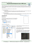
Using Spatial Analyst functions you can create a rich set of informative maps from your data. Create a hillshade to use as a backdrop of
the terrain to support other data layers. Calculate slope, aspect, and contours, or create a map displaying visibility. Use derived data
together to help solve spatial problems.
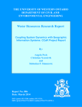
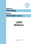
In order to break a suspect’s alibi, a viewshed analysis finds out if he actually would have been able to see the location of the
fire from where he called it in, claiming he saw flames. Areas drawn in yellow identify the locations from which the fire would
have been seen. This visibility analysis demonstrates that he could not have seen the flames from the phone booth.
4
USING ARCGIS SPATIAL ANALYST
Identifying spatial relationships
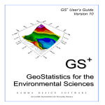
Spatial Analyst provides tools to model spatial relationships.
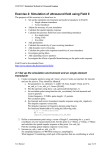
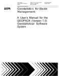
Model results aid in visual analysis. The darker red areas show locations predicting the highest level of drug traffic while the yellow dots
represent the drug arrest locations for a three-month period. There is a high correlation between the two. There is also a marked
difference in the number of arrests when you go west of 16th Street.
INTRODUCING ARCGIS SPATIAL ANALYST
5
Finding suitable locations
Use the Spatial Analyst to query your data to identify locations that meet your set of objectives or produce a suitability map, combining
datasets to analyze suitability.
Suitable locations for winter rock climbing, based on distance from a campsite and steep, south-facing slopes
6
USING ARCGIS SPATIAL ANALYST
Calculating cost of travel
Travel cost analysis involves modeling to generate the cost surface and then calculating optimum corridors across the surface.
Calculating travel cost can provide a rich set of information for decision making.
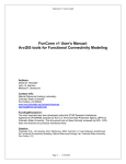
Haul Cost Analysis
Boise Cascade Corporation,
Boise, Idaho
Brian Liberty, Nick Blacklock
Copyright @ 1997
This map displays the least-cost travel for timber transport within a 200-mile radius of each mill. It considers obstacles to
travel and estimates the cost in dollars to transport wood from each location to the nearest mill.
INTRODUCING ARCGIS SPATIAL ANALYST
7
Tips on learning Spatial Analyst
About this book
If you’re new to the concept of geographic information systems
(GIS), remember that you don’t have to know everything about
Spatial Analyst to get immediate results. Begin learning Spatial
Analyst by reading Chapter 2, ‘Quick-start tutorial’. This chapter
introduces you to some of the tasks you can accomplish using
Spatial Analyst and provides an excellent starting point as you
start to think about how to tackle your own spatial problems.
Spatial Analyst comes with the data used in the tutorial, so you
can follow along step by step at your computer.
This book is designed to help you perform spatial analysis by
giving you conceptual information and teaching you how to
perform tasks to solve your spatial problems. Topics covered in
Chapter 2, ‘Quick-start tutorial’, assume you are familiar with the
fundamentals of GIS and have a basic knowledge of ArcGIS. If
you are new to GIS or ArcMap™, you are encouraged to take
some time to read Getting Started with ArcGIS and Using
ArcMap, which you received in your ArcGIS package. It is not
necessary to do so to continue with this book; simply use these
books as references.
If you prefer to jump right in and experiment on your own, use
Chapter 7, ‘Performing spatial analysis’, as a guide to learn the
concepts and the steps to perform a certain task.
Finding answers to questions
Like most people, your goal is to complete your tasks while
investing a minimum amount of time and effort on learning how to
use software. You want intuitive, easy-to-use software that gives
you immediate results without having to read pages of
documentation. However, when you do have a question, you
want the answer quickly so you can complete your task. That’s
what this book is all about—getting the answers you need, when
you need them.
This book describes spatial analysis tasks—from basic to
advanced—that you’ll perform using Spatial Analyst. Although
you can read this book from start to finish, you’ll likely use it
more as a reference. When you want to know how to perform a
particular task, such as finding the shortest path, just look it up in
the table of contents or the index. What you’ll find is a concise,
step-by-step description of how to complete the task. Some
chapters also include detailed information that you can read if
you want to learn more about the concepts behind the tasks. You
may also refer to the glossary in this book if you come across any
unfamiliar GIS terms or need to refresh your memory.
8
Chapter 3, ‘Modeling spatial problems’, takes you through the
spatial modeling process, helping you to break down your spatial
problems into manageable pieces. Chapter 4, ‘Understanding
raster data’, helps you to understand raster data, and Chapter 5,
‘Understanding cell-based modeling’, explains the process of cellbased modeling. Chapter 6, ‘Setting up your analysis
environment’, tells you how to set up your analysis options
before performing analysis, and Chapter 7, ‘Performing spatial
analysis’, provides detailed information to help you perform each
spatial function.
The appendices are split into three sections: Appendix A explains
Map Algebra syntax and rules for the Raster Calculator,
Appendix B provides a table of supported operators and
precedence values for use in the Raster Calculator, and
Appendix C explains remap tables for use when reclassifying data
using the Raster Calculator.
Getting help on your computer
In addition to this book, use the ArcGIS Desktop Help system to
learn how to use Spatial Analyst and ArcMap. To learn how to
use the ArcGIS Desktop Help system, see Using ArcMap.
USING ARCGIS SPATIAL ANALYST
Contacting ESRI
If you need to contact ESRI for technical support, see the product
registration and support card you received with ArcGIS Spatial
Analyst, or refer to ‘Contacting Technical Support’ in the ‘Getting
more help’ section of the ArcGIS Desktop Help system. You can
also visit ESRI on the Web at www.esri.com and support.esri.com
for more information on Spatial Analyst and ArcGIS.
ESRI education solutions
ESRI provides educational opportunities related to geographic
information science, GIS applications, and technology. You can
choose among instructor-led courses, Web-based courses, and
self-study workbooks to find education solutions that fit your
learning style. For more information, go to www.esri.com/
education.
INTRODUCING ARCGIS SPATIAL ANALYST
9
2
Quick-start tutorial
IN THIS CHAPTER
• Exercise 1: Displaying and
exploring your data
• Exercise 2: Finding a site for a
new school
• Exercise 3: Finding an alternative
route to the new school site
With Spatial Analyst you can easily perform spatial analysis on your data.
You can provide answers to simple spatial questions, such as “How steep is
it at this location?” or “What direction is this location facing?”, or you can
find answers to more complex spatial questions, such as “Where is the best
location for a new facility?” or “What is the least-cost path from A to B?”
When used in conjunction with ArcMap, Spatial Analyst provides a comprehensive set of tools for exploring and analyzing your spatial data, enabling
you to find solutions to your spatial problems.
Tutorial scenario
The town of Stowe, Vermont, USA, has experienced a substantial increase
in population. Demographic data suggests this increase has occurred due to
families with children moving to the region, taking advantage of the many
recreational facilities located nearby. It has been decided that a new school
must be built to take the strain off the existing schools, and as a town
planner you have been assigned the task of finding the potential sites.
Spatial Analyst provides the tools to find an answer to such spatial problems. This tutorial will show you how to use some of these tools and will
give you a solid basis from which you can start to think about how to solve
your own specific spatial problems.
11
Ch02.pmd
11
2003.11.17, 11:13
It is assumed that you have installed the Spatial Analyst
extension before you begin this tutorial. The data required
is included on the Spatial Analyst installation disk (the
default installation path is ArcGIS\ArcTutor\Spatial, on the
drive where the tutorial data is installed). The datasets were
provided courtesy of the State of Vermont for use in this
tutorial. The tutorial scenario is fictitious, and the original
data has been adapted for the purpose of the tutorial.
The datasets are:
Dataset
Description
Elevation
Raster dataset of the elevation of the area
Landuse
Raster dataset of the landuse types over the
area
Roads
Feature dataset displaying linear road
network
Rec_sites
Feature dataset displaying point locations
of recreation sites
Schools
Feature dataset displaying point locations
of existing schools
Destination
Feature dataset displaying the destination
point for use in finding the shortest path
In this tutorial you will first explore your data to learn
more about it and to understand its relationships. Then, you
will find suitable locations for the new school, based on the
fact that it is preferable to locate close to recreational
facilities for ease of access to these places for the children,
and it is also important to locate away from existing
schools to spread their locations over the town. You also
want to avoid steep slopes and certain landuse types.
12
Once you have found the best sites, you will examine these
locations to see which is potentially the most suitable. You
will then examine the data to see if any problems may arise
from building the school in the chosen location.
This tutorial is divided into exercises and is designed to let
you explore the functionality of Spatial Analyst at your
own pace.
• Exercise 1 shows you how to display and explore your
data using the functionality of ArcMap and Spatial
Analyst. You will add and display your datasets, highlight values on the map, identify locations to obtain
values, examine a histogram, and create a hillshade.
• Exercise 2 helps you to find the best location for a new
school by creating a suitability map. You will derive
datasets of distance and slope, reclassify datasets to a
common scale, weight those that are more important to
consider, then combine the datasets to find the most
suitable locations.
• Exercise 3 shows you how to find an alternative route—
the least-cost, or shortest path—for a road to the new
school site.
Copies of the results obtained from each exercise are stored
in the Results folder on your local drive where you installed the tutorial data (the default installation path is
ArcGIS\ArcTutor\Spatial\Results).
You will need about one hour of focused time to complete
the tutorial. However, you can perform the exercises one at
a time if you wish, saving your results along the way when
recommended.
USING ARCGIS SPATIAL ANALYST
Exercise 1: Displaying and exploring your data
You should explore your data to understand it and to identify
relationships. Understanding your data and recognizing
relationships will enable you to more accurately prepare
your data for analysis.
In this exercise, you will open ArcMap and add the Spatial
Analyst toolbar to your ArcMap session. You will then
explore your datasets using functionality within ArcMap
and Spatial Analyst.
3
Starting ArcMap and Spatial Analyst
1. Start ArcMap by either double-clicking a shortcut
installed on your desktop or using the Programs list in
your Start menu.
The Spatial Analyst toolbar is added to your ArcMap
session.
2. Click OK to open a new empty map.
Enabling the Spatial Analyst toolbar
1. Click the Tools menu.
2. Click Extensions and check Spatial Analyst.
3. Click Close.
2
3. Click View, point to Toolbars, and click Spatial Analyst.
QUICK-START TUTORIAL
13
Adding data to your ArcMap session
1. Click the Add Data button on the Standard toolbar.
The datasets are added to the ArcMap table of contents as layers.
1
2. Navigate to the folder on your local drive where you
installed the tutorial data (the default installation path is
ArcGIS\ArcTutor\Spatial, on the drive where the tutorial
data is installed).
3. Click elevation, press and hold down the Shift key, then
click landuse, rec_sites, roads, and schools.
4. Click Add.
3
You will now explore the display capabilities of ArcMap by
changing the symbology of some of the layers.
1. Right-click landuse in the table of contents and click
Properties.
2
4
14
Displaying and exploring data
1
USING ARCGIS SPATIAL ANALYST
2. Click the Symbology tab.
All landuse categories are currently drawn using cell
values as the Value Field and in random colors. You will
change the Value Field to be more meaningful and
change the color of each symbol to show a more
appropriate color for each landuse on the map.
You can also change the color and properties of symbols via
the table of contents.
6. Click the point representing schools in the table of
contents.
3. Click the Value Field dropdown arrow and click landuse.
6
4. Double-click each symbol and choose a suitable color to
represent each landuse type.
5. Click OK.
7. Scroll to the School 2 symbol and click it.
8. Click the color dropdown arrow and click a color.
2
3
9. Click OK.
8
4
The changes you make are reflected in the table of
contents and in the map.
QUICK-START TUTORIAL
7
9
The changes you make are reflected in the table of
contents and in the map.
15
Highlighting a selection on the map
Examining the attribute table gives you an idea of the
number of cells of each attribute in the dataset.
1. Right-click landuse in the table of contents and click
Open Attribute Table.
1
Notice that Forest (value of 6) has the largest count,
followed by Agriculture (value of 5), then Water
(value of 2).
2. Click the row representing Wetlands (value of 7).
16
2
This selected set, all areas of Wetlands, is highlighted on
the map.
3. Click the Options button on the Open Attribute Table
dialog box, then click Clear Selection.
3
4. Click the Close button to close the Attributes of landuse
table.
USING ARCGIS SPATIAL ANALYST
5
Identifying features on the map
3
6
1. Click the Identify tool on the Tools toolbar.
2. Click the Rec_site shown in the map below to identify
the features in this particular location.
2
1
Using Spatial Analyst to explore your data
You will now create a histogram from the landuse layer
and a hillshade from the Elevation layer to gain more of an
understanding of the nature of the landscape.
Setting the analysis properties
Before you use Spatial Analyst, you should set up the
analysis options, stating the working directory, the extent,
and the cell size for your analysis results. These settings
are specified in the Options dialog box.
Note: Your display will not be zoomed in this much; this
is only to show the location of the recreation site to
click.
3. Click the Layers dropdown arrow on the Identify
Results dialog box and click All layers.
4. Click the Rec_site again to identify the features in this
particular location for all layers.
5. Expand the tree of each layer to obtain the value for
each layer in this location.
6. Close the Identify Results dialog box.
QUICK-START TUTORIAL
17
1. Click the Spatial Analyst dropdown arrow and click
Options.
2
1
2. Specify a working directory on your local drive in which
to place your analysis results. For example, type
c:\spatial to create a folder called spatial on your C:\
drive for use throughout this tutorial.
3
4
3. Click the Extent tab.
4. Click the Analysis extent dropdown arrow and click
Same as Layer “landuse”.
The extent of all subsequent resulting datasets will be
the same as the landuse layer.
18
USING ARCGIS SPATIAL ANALYST
5. Click the Cell Size tab.
Creating a hillshade
6. Click the Analysis Cell Size dropdown arrow and click
Same as Layer “elevation”.
Creating a hillshade from elevation data and adding transparency gives you a good visual impression of the terrain
and can greatly enhance the display of your map.
7. Click OK on the Options dialog box.
This will set the cell size for your analysis results to be at
a 30-meter resolution, the largest cell size of your
datasets.
1. Click the Spatial Analyst dropdown arrow, point to
Surface Analysis, and click Hillshade.
Examining a histogram
1. Click the Layer dropdown arrow and click landuse.
2. Click the Histogram button.
1
1
2
The histogram displays the number of cells of each type
of landuse.
3. Close the Histogram.
QUICK-START TUTORIAL
2. Click the Input surface dropdown arrow and click
elevation. Leave the defaults for all other options.
2
19
3. Click OK on the Hillshade dialog box.
The result of the Hillshade function is added to the map
as a new layer.
4
5
All results from analysis functions are temporary. If you
want to make any result available for future use, you
should make the dataset permanent.
4. Right-click the created hillshade layer and click Make
Permanent.
5. Navigate to the folder on your local drive where you set
up your working directory (C:\Spatial).
6. Type “Hillshade” in the Name text box.
8
7. Click the Save as type dropdown arrow and click ESRI
GRID.
8. Click Save.
Note: A copy of Hillshade can be found in the location
ArcGIS\ArcTutor\Spatial\Results\Ex1\Hillshade on the
drive where the tutorial data is installed.
20
6
7
USING ARCGIS SPATIAL ANALYST
Applying transparency
You will now make the landuse layer transparent so the
Hillshade can be seen through it.
1. Click Hillshade of elevation in the table of contents and
drag the layer below the landuse layer.
2
1
2. Click View on the Main menu, point to Toolbars, and
click Effects.
3. Click the Layer dropdown arrow and click landuse.
4. Click the Adjust Transparency button and move the
scroll bar up to 30 percent transparency.
3
4
The Hillshade layer can now be seen underneath the
landuse layer, giving a vivid impression of the terrain.
QUICK-START TUTORIAL
21
5
6
Exploring your data gives you a useful basis of information that will help you during your analysis. For example, you need to know the different landuse types and
their distribution over an area, as well as their relative
importance, in order to decide how much weight each
should have in a suitability model. Alternatively, you
need to know how rugged the terrain is so you know to
include slope as a factor in determining the least-cost
path.
Having explored your data, you are now in a position to
begin to find suitable locations for the new school.
First, you will need to remove all the layers used in this
exercise.
5. Click the top layer in the table of contents to highlight
it. Press and hold the Shift key and click all other layers.
6. Right-click one of the layers in the table of contents and
click Remove.
22
All layers will be removed from the ArcMap data
frame.
This exercise showed you how to display and explore your
data. In the next exercise you will use the Spatial Analyst
functions to find a potential site for a new school. You can
continue on with the tutorial or close ArcMap and continue
at a later date. There is no need to save the map document
at this point.
Note: To save your work at any time, click the File menu
and click Save As. Navigate to the location where you set
up your local working directory (C:\Spatial), specify a
filename for the map document—Spatial_Tutorial—and
click Save. Simply open Spatial_Tutorial.mxd when you
wish to continue with the tutorial. You will, however, be
prompted when it is appropriate to save the map document.
USING ARCGIS SPATIAL ANALYST
Exercise 2: Finding a site for a new school in Stowe, Vermont, USA
In this exercise you will find suitable locations for a new
school. The four steps to produce such a suitability map are
outlined below.
Step 1:
Input Datasets
Step 2:
Derive Datasets
Step 3:
Reclassify
Datasets
Step 4:
Weight and
Combine
Datasets
Landuse
Decide which datasets you need as
inputs. The datasets you will use in
this exercise are displayed to the
right.
Reclassify each dataset to a common scale—for example, 1–10—
giving higher values to more suitable
attributes.
Weight datasets that should have
more influence in the suitability
model if necessary, then combine
them to find the suitable locations.
Elevation
Recreation
Schools
Step 2
Calculate Slope Find Distance Find Distance
Derive datasets. Create data from
existing data to gain new information.
Your input datasets in this exercise are Landuse, Elevation,
Recreation Sites, and Existing Schools. You will derive
slope, distance to recreation sites, and distance to existing
schools, then reclassify these derived datasets to a common
scale from 1–10. You will then weight them according to a
percentage influence and combine them to produce a map
displaying suitable locations for the new school. The
diagram to the right shows the process you will take.
QUICK-START TUTORIAL
Step 1
Step 3
Reclassify
Reclassify
Reclassify
Reclassify
Step 4
Weight and Combine Datasets
23
Step 1: Inputting datasets
1. Click the Add Data button on the Standard toolbar.
Setting the analysis properties
Set up the analysis options like you did in Exercise 1.
1. Click the Spatial Analyst dropdown arrow and click
Options.
1
2. Navigate to the folder on your local drive where you
installed the tutorial data (the default installation path is
ArcGIS\ArcTutor\Spatial, on the drive where the tutorial
data is installed).
3. Click elevation, then click and hold down the Ctrl key
and click landuse, rec_sites, and schools.
4. Click Add.
3
2. Specify a working directory on your local drive in
which to place your analysis results. Type c:\spatial to
create a folder called spatial on your C:\ drive.
3. Click the Extent tab.
4. Click the Analysis Extent dropdown arrow and click
Same as Layer “landuse”.
5. Click the Cell Size tab.
6. Click the Analysis Cell Size dropdown arrow and click
Same as Layer “elevation”.
7. Click OK on the Options dialog box.
2
4
Each dataset is added to the ArcMap table of contents
as a layer.
24
USING ARCGIS SPATIAL ANALYST
Step 2: Deriving datasets
Deriving data from your input datasets is the next step in
the suitability model. You will derive the following:
• Slope from elevation
3. Type slope in the Output raster text box to permanently
save your output slope dataset to the location of your
working directory (c:\spatial).
You will use this dataset again in Exercise 3.
• Distance from recreation sites
• Distance from existing schools
Note: A copy of this slope dataset can be found in the
location ArcGIS\ArcTutor\Spatial\Results\Ex2\Slope.
Deriving slope
4. Click OK.
Since the area is mountainous, you need to find areas of
relatively flat land to build on, so you will take into consideration the slope of the land.
2
1. Click the Spatial Analyst dropdown arrow, point to
Surface Analysis, and click Slope.
1
3
4
The output slope dataset will be added to your ArcMap
session as a new layer. High values—red areas—
indicate steeper slopes.
2. Click the Input surface dropdown arrow and click
elevation.
QUICK-START TUTORIAL
25
3. Click OK.
2
Deriving distance from recreation sites
In this model, it is preferable that the school be built near
recreational facilities, so you will now calculate the
straight-line distance from Recreation Sites.
1. Click the Spatial Analyst dropdown arrow, point to
Distance, and click Straight Line.
3
The output distance to the rec_sites dataset will be
added to your ArcMap session as a new layer. Values of
zero indicate the location of a recreation site, with
values—distances—increasing as you move away from
each of these sites.
1
2. Click the Distance to dropdown arrow and click
rec_sites.
Leave the defaults for all other options.
26
USING ARCGIS SPATIAL ANALYST
Note: A copy of this distance to rec_sites dataset can be
found in the location
ArcGIS\ArcTutor\Spatial\Results\Ex2\recD.
The output distance to schools dataset will be added to
your ArcMap session as a new layer.
4. Uncheck the box next to Schools to turn off this layer so
you only see the locations of the recreation sites and the
distance to them.
Deriving distance from schools
You will now derive a dataset of distance from existing
schools. It is preferable to locate the new school away from
existing schools to spread out their locations through the
town.
1. Click the Spatial Analyst dropdown arrow, point to
Distance, and click Straight Line.
2. Click the Distance to dropdown arrow and click schools.
Leave the defaults for all other options.
3. Click OK.
2
4. Check the box next to the schools layer to turn it back
on and uncheck the box next to rec_sites to turn this
layer off so you only see the locations of the schools and
the distance to them.
Note: A copy of this distance to schools dataset can be
found in the location
ArcGIS\ArcTutor\Spatial\Results\Ex2\schD.
3
QUICK-START TUTORIAL
27
Step 3: Reclassifying datasets
You now have the required datasets to find the best location
for the new school. The next step is to combine them to
find out where the potential locations can be found.
In order to combine the datasets, they must first be set to a
common scale. That common scale is how suitable a
particular location—each cell—is for building a new school.
You will reclassify each dataset to a common scale, within
the range 1–10, giving higher values to attributes within
each dataset that are more suitable for locating the school:
1
• Reclassify slope
• Reclassify Distance to recreation sites
• Reclassify Distance to schools
• Reclassify landuse
2
Reclassifying slope
It is preferable that the new school site be located on
relatively flat ground. You will reclassify the Slope layer,
giving a value of 10 to the most suitable slopes—those with
the lowest angle of slope—and 1 to the least suitable
slopes—those with the steepest angle of slope.
3
1. Click the Spatial Analyst dropdown arrow and click
Reclassify.
2. Click the Input raster dropdown arrow and click Slope.
3. Click Classify.
28
USING ARCGIS SPATIAL ANALYST
4. Click the Method dropdown arrow and click Equal
Interval.
7
5. Click the Classes dropdown arrow and click 10.
6. Click OK.
5
4
8
6
You want to reclassify the Slope layer so steep slopes
are given low values, as these are least suitable for
building on.
The output reclassified slope dataset will be added to your
ArcMap session as a new layer. Locations with higher
values—less-steep slopes—are more suitable than locations
with lower values—steeper slopes.
7. Click the first New value record in the Reclassify dialog
box and change it to a value of 10. Give a value of 9 to
the next New value, 8 to the next, and so on. Leave
NoData as NoData.
8. Click OK.
QUICK-START TUTORIAL
29
Note: A copy of this reclassified slope dataset can be found
in the location
ArcGIS\ArcTutor\Spatial\Results\Ex2\slopeR.
2
Reclassifying distance to recreation sites
3
The school should be located near recreational facilities.
You will reclassify this dataset, giving a value of 10 to
areas closest to recreation sites—the most suitable locations—giving a value of 1 to areas far from recreation
sites—the least suitable locations—and ranking the values
in between. By doing this you will find out which areas are
near and which areas are far from recreation sites.
1. Click the Spatial Analyst dropdown arrow and click
Reclassify.
4. Click the Method dropdown arrow and click Equal
Interval.
5. Click the Classes dropdown arrow and click 10.
6. Click OK.
5
4
1
2. Click the Input raster dropdown arrow and click
Distance to rec_sites.
3. Click Classify.
6
30
USING ARCGIS SPATIAL ANALYST
You want to locate the school near recreational facilities,
so you will give higher values to locations close to
recreational facilities, as these are the most desirable.
7. As you did when reclassifying the Slope layer, click the
first New value record in the dialog box and change it to
a value of 10. Give a value of 9 to the next New value, 8
to the next, and so on. Leave NoData as NoData.
The output reclassified distance to recreation sites
dataset will be added to your ArcMap session as a new
layer. It shows locations that are more suitable for
locating another school. High values indicate more
suitable locations.
8. Click OK.
7
Note: A copy of this reclassified distance from recreation
sites dataset can be found in the location
ArcGIS\ArcTutor\Spatial\Results\Ex2\recR.
8
QUICK-START TUTORIAL
31
2
Reclassifying distance to schools
It is necessary to locate the new school away from existing
schools in order to avoid encroaching on their catchment
areas. You will reclassify the Distance to schools layer,
giving a value of 10 to areas away from existing schools—
the most suitable locations—giving a value of 1 to areas
near existing schools—east suitable locations—and ranking
the values in between. By doing this you will find out
which areas are near and which areas are far from existing
schools.
3
1. Click the Spatial Analyst dropdown arrow and click
Reclassify.
4. Click the Method dropdown arrow and click Equal
Interval.
5. Click the Classes dropdown arrow and click 10.
6. Click OK.
1
5
4
2. Click the Input raster dropdown arrow and click
Distance to schools.
3. Click Classify.
6
32
USING ARCGIS SPATIAL ANALYST
You want to locate the school away from existing
schools, so you will give higher values to locations
farther away, as these locations are most desirable.
As the default gives high New values—more suitable—
to high Old values—locations farther away from existing
schools—you do not need to change any values this
time.
7. Click OK.
Note: A copy of this reclassified distance from schools
dataset can be found in the location
ArcGIS\ArcTutor\Spatial\Results\Ex2\schR.
7
The output reclassified distance to schools dataset will
be added to your ArcMap session as a new layer. It
shows locations that are more suitable for locating
another school. Higher values indicate more suitable
locations.
QUICK-START TUTORIAL
33
Reclassifying landuse
At a town planners meeting it was decided that certain
landuse types were better for building on than others,
taking into consideration the costs involved in building on
different landuse types.
You will now reclassify landuse. A lower value indicates
that a particular landuse type is less suitable for building
on. Water and Wetlands will be given NoData as they
cannot be built on and should be excluded.
You will now remove the Water and Wetland attributes
and change their values to NoData.
5. Click the row for Water, press the Shift key, click
Wetlands, then click Delete Entries.
6. Check Change missing values to NoData.
All values for Water and Wetlands will be changed to
NoData.
7. Click OK.
1. Click the Spatial Analyst dropdown arrow and click
Reclassify.
4
2
3
5
1
2. Click the Input raster dropdown arrow and click landuse.
3. Click the Reclass field dropdown arrow and click
Landuse.
6
7
4. Type the following values in the New values column:
Agriculture—10
Built up—3
Barren land—6
Forest—4
Brush/Transitional—5
34
USING ARCGIS SPATIAL ANALYST
The output reclassified landuse dataset will be added to
your ArcMap session as a new layer. It shows locations
that have landuse types that are considered to be better
than others for locating the school—higher values
indicate more suitable locations.
9
W
Q
Note: A copy of this reclassified landuse dataset can be
found in the location
ArcGIS\ArcTutor\Spatial\Results\Ex2\landuseR.
8. Right-click Reclass of landuse in the table of contents
and click Properties.
9. Click the Symbology tab.
10. Click the Display NoData as dropdown arrow and click
Arctic White to show NoData values—Water and
Wetlands—in this color.
11. Click OK.
QUICK-START TUTORIAL
35
Step 4: Weighting and combining datasets
After applying a common scale to your datasets, where
higher values are given to those attributes that are considered more suitable within each dataset, you are ready to
combine them to find the most suitable locations.
If all datasets were equally important, you could simply
combine them at this point; however, you have been
informed that it is preferable to locate the new school close
to recreational facilities and away from other schools. You
will weight all the datasets, giving each a percentage
influence. The higher the percentage, the more influence a
particular dataset will have in the suitability model.
You will give the layers the following percent influence:
(Each percentage is divided by 100 to normalize the
values.)
Reclass of Distance to rec_sites:
0.5
(50%)
Reclass of Distance to schools:
0.25
(25%)
Reclass of landuse:
0.125
(12.5%)
Reclass of slope:
0.125
(12.5%)
1. Click the Spatial Analyst dropdown arrow and click
Raster Calculator.
1
2. Double-click Reclass of Distance to rec_sites from the
Layers list to add it to the expression box.
3. Click Multiply.
4. Click 0.5.
5. Click Add.
6. Double-click Reclass of Distance to schools.
7. Click Multiply.
8. Click 0.25.
9. Click Add.
10. Double-click Reclass of landuse.
11. Click Multiply.
12. Click 0.125.
13. Click Add.
14. Double-click Reclass of slope.
15. Click Multiply.
36
USING ARCGIS SPATIAL ANALYST
16. Click 0.125.
17. Click Evaluate to perform the weighting and combining
of the datasets.
18. Right-click the newly created raster layer in the table of
contents and click Properties.
19. Click the Symbology tab.
20. Click Classified from the Show list.
21. Click the Classes dropdown arrow and click 10.
22. Scroll to the last three classes, click one, then press and
hold the Shift key and click the other two.
23. Right-click the highlighted classes, click Properties for
selected Colors, and click a bright color.
24. Click the Display NoData as dropdown arrow and click
the color black. This displays values of NoData—Water
and Wetlands—in this color.
25. Click OK.
A
S
P
I
The output raster dataset shows you how suitable each
location is for locating the new school, according to the
criteria you set in the suitability model. Higher values
indicate locations that are more suitable.
The suitable locations are those areas that are close to
recreation sites, away from existing schools, on relatively flat land, and on certain types of landuse. The
higher weightings set for Distance to schools and
Distance to rec_sites have a powerful influence on
deciding which areas are more suitable than others.
QUICK-START TUTORIAL
D
G
F H
37
You decide that there are three main potential areas for
locating the school. They are labeled in the diagram
below.
Area 1
Area 2
Area 3
Note: A copy of this Suitability dataset can be found in
the location
ArcGIS\ArcTutor\Spatial\Results\Ex2\Suitability.
29. Click the output raster twice slowly. Rename the layer
Suitability.
Z
You decide that the best location is somewhere within Area
1, as there are three recreation sites in the neighboring area,
the ski resort being one of them. Also, although you know
that a considerable volume of traffic already uses the
current access road to this potential site, you are involved
in plans for constructing an alternative road to this area,
which will help alleviate the volume of traffic on the
current access road.
You should now assess these locations to see which
might be the best location. This should be done in the
field, as well as by examining the data you have on each
potential area.
26. Right-click the output layer in the table of contents and
click Make Permanent.
27. Navigate to the folder on your local drive where you set
up your working directory (c:\spatial).
28. Type Suitability and click Save.
The temporarily created dataset will now be permanently stored on disk.
38
30. Click the Schools layer in the table of contents, press
the Ctrl key, and click all other layers except Suitability
(use the scroll bar to move down the table of contents).
31. Right-click one of the highlighted layers and click
Remove.
You have now completed Exercise 2. You can continue on
to Exercise 3, or you can stop and continue later. Whichever option you choose, save the map document at this
point. Click the File menu and click Save As. Navigate to
the location where you set up your local working directory
(c:\spatial), specify a filename for the map document—
Spatial_Tutorial—and click Save.
USING ARCGIS SPATIAL ANALYST
Exercise 3: Finding an alternative access road to the new school site
In this exercise you will find the best route for a new
access road. The steps you might follow to produce such a
path are outlined below, and the steps you will take in this
exercise are diagrammed to the right.
Step 1: Create Source and Cost Datasets
Source
Cost
Step 1: Create Source and Cost Datasets
Create the source dataset if necessary. The Source is the
school site in this exercise.
Create the cost dataset by deciding which datasets are
required, reclassifying them to a common scale, weighting,
then combining them.
Step 2: Cost Weighted Distance
Step 2: Perform Cost Weighted Distance
Perform cost weighted distance using the Source and Cost
datasets as inputs. The Distance dataset created from this
function is a raster where the value of each cell is the
accumulated cost of traveling from each cell back to the
source.
To find the shortest path, you need a Direction dataset,
which can be created as an additional dataset from the cost
weighted function. This gives you a raster of the direction
of the least costly path from each cell back to the source (in
this exercise, the school site).
Destination
Distance
Direction
Step 3: Shortest Path
Step 3: Perform Shortest Path
Create the destination dataset if necessary. In this exercise,
the Destination is a point at a road junction.
Perform shortest path using the Distance and Direction
datasets created from the cost weighted function.
QUICK-START TUTORIAL
39
Step 1: Creating the source and cost datasets
To find the best route to the potential school site, you will
first need to create the Source dataset (the school site)
from the suitability map, and a Cost dataset, and use these
as inputs into the cost weighted function.
3
Creating the source dataset
If you want to know how to create the Source dataset,
follow the next 29 steps. Alternatively, click the Add Data
button and navigate to the location where you installed the
tutorial data (ArcGIS\ArcTutor\Spatial). Click Roads, then
click Add. Then, click the Add Data button again and
navigate to ArcGIS\ArcTutor\Spatial\Results\Ex3. Click
School_site, then click Add and skip the next 29 steps.
You will first create an empty shapefile in ArcCatalog™,
then digitize the location of the site using the editng tools in
ArcMap.
1. Click the ArcCatalog button on the Standard toolbar.
4. Type “School_site” for the name of the new shapefile.
5. Click the Feature Type dropdown arrow and click
Polygon to choose the type of feature that will be
created.
6. Click Edit to add spatial reference information to the
shapefile.
4 5
1
2. Navigate in the Catalog tree to the folder on your local
drive where you set up your working directory
(c:\spatial).
6
3. Right-click the Spatial folder, point to New, and click
Shapefile.
40
USING ARCGIS SPATIAL ANALYST
7. Click Select to use a predefined coordinate system.
10. Click OK on the Spatial Reference Properties dialog
box.
11. Click OK on the Create New Shapefile dialog box.
A new shapefile called School_site will be created and
added to the Catalog tree.
12. Click File, click Exit to close ArcCatalog, and return to
ArcMap.
13. Click the Add Data button and navigate to the folder on
your local drive where you installed the tutorial data
(the default installation path is
ArcGIS\ArcTutor\Spatial).
7
14. Click roads.shp.
15. Click Add.
8. Click the Projected Coordinate Systems folder, click
State Plane, then click NAD 1983 and scroll to NAD
1983 StatePlane Vermont FIPS 4400.prj.
T
R
9. Click Add.
8
Y
9
16. Click the Add Data button again and navigate to the
folder on your local drive where you set up your
working directory (c:\spatial).
17. Click School_site.
18. Click Add.
QUICK-START TUTORIAL
41
19. Click the Zoom In tool on the Tools toolbar and zoom in
on the area that was deemed most suitable (area 1,
circled in yellow below).
20. Click View, point to Toolbars, and click Editor.
P
A
21. Click the Editor dropdown arrow and click Start
Editing.
S
42
USING ARCGIS SPATIAL ANALYST
22. Click c:\spatial (or wherever you specified your working
directory to be) for the folder from which to edit data.
28. Click the Editor dropdown arrow and click Stop Editing.
23. Click OK.
Note: A copy of this school_site dataset can be found in the
location ArcGIS\ArcTutor\Spatial\Results\Ex3\source.shp.
24. Click the Task dropdown arrow and click Create New
Feature.
25. Click the Target dropdown arrow and click School_site.
26. Click the Create New Feature dropdown arrow and
click Create New Feature.
J
G
H
29. Click Yes to save your edits.
Creating the cost dataset
You will now create a dataset of the cost of traveling over
the landscape, based on the fact that it is more costly to
traverse steep slopes and construct a road on certain
landuse types.
1. Right-click the Suitability layer and click Remove.
2. Click the Add Data button and navigate to the folder on
your local drive where you set up your working directory
(c:\spatial).
3. Click slope (the dataset created in exercise 2).
27. Draw a polygon on the screen in the location shown in
the diagram. Click and hold to add a polygon vertex,
drag the cursor, and add another polygon vertex.
Continue until the polygon is complete. Double-click to
close the polygon.
4. Click Add.
5. Click the Add Data button again and navigate to the
folder on your local drive where you installed the
tutorial data (the default installation path is
ArcGIS\ArcTutor\Spatial).
6. Click landuse and click Add.
K
QUICK-START TUTORIAL
43
7. Right-click landuse and click Zoom To Layer.
2. Click the Input raster dropdown arrow and click slope.
3. Click Classify.
2
7
3
Reclassifying slope
1. Click the Spatial Analyst dropdown arrow and click
Reclassify.
4. Click the Method dropdown arrow and click Equal
Interval.
5. Click the Classes dropdown arrow and click 10.
6. Click OK.
1
44
USING ARCGIS SPATIAL ANALYST
5
4
6
You want to avoid steep slopes when constructing the
road, so steep slopes should be given higher values in
the Cost dataset.
Reclassifying landuse
1. Click the Spatial Analyst dropdown arrow and click
Reclassify.
As the defaults give high values to steeper slopes, you
do not need to change the default New Values.
7. Click OK on the Reclassify dialog box.
The Reclass of slope layer will be added to the table of
contents. It shows locations that are more costly than
others for constructing a road—higher values indicate
the more costly areas that should be avoided.
QUICK-START TUTORIAL
1
45
2. Click the Input raster dropdown arrow and click landuse.
3 Click the Reclass field dropdown arrow and click
Landuse.
4. Click the first New value to edit the values and type in
the following values:
Agriculture—4
Built up—9
Barren land—6
Forest—8
Brush/Transitional—5
Water—10
The Reclass of landuse layer will be added to the table of
contents. It shows locations that are more costly than others
for constructing a road, based on the type of landuse.
The NoData value—Wetlands—is currently displayed
transparently so you can see the layers underneath. To
make this value solid, change it to white.
8. Right-click Reclass of landuse and click Properties.
9. Click the Symbology tab.
Higher values indicate higher road-construction costs.
5. Click Wetlands and click Delete Entries.
10. Click the Display NoData as dropdown arrow and click
Arctic White.
11. Click OK.
6. Click Change missing values to NoData.
9
7. Click OK.
2
4
3
Q
5
W
6
46
7
USING ARCGIS SPATIAL ANALYST
1
Combining datasets
You will now combine Reclass of slope and Reclass of
landuse in order to produce a dataset of the cost of building
a road at each location in the landscape, in terms of steepness of slope and landuse type. In this model, each dataset
has equal weighting, so it is not necessary to apply any
weight as we did when finding the suitable location for the
school.
2
4 3
1. Click the Spatial Analyst dropdown arrow and click
Raster Calculator.
2. Double-click Reclass of landuse to add it to the
expression box.
3. Click the Add button.
4. Double-click Reclass of slope to add it to the expression
box.
5. Click Evaluate.
QUICK-START TUTORIAL
5
47
The result is added to your ArcMap session. Locations
with low values identify the areas that will be the least
costly to build a road through. They are displayed in
dark blue in the graphic below.
Step 2: Performing cost weighted distance
You will now perform cost weighted distance using the Cost
dataset you just created and the School_site layer (the
source). Using this function, you will create a Distance
dataset where each cell contains a value representing the
accumulated least cost of traveling from that cell to the
school site and a Direction dataset that gives the direction
of the least-cost path from each cell back to the source.
This conceptual process is explained in more detail in
Chapter 7, ‘Performing spatial analysis’.
1. Click the Spatial Analyst dropdown arrow, point to
Distance, and click Cost Weighted.
6. Click the output layer in the table of contents to highlight
it, click again, and rename it Cost.
1
You will now remove all layers except Cost,
School_site, and Roads.
7. Click Reclass of landuse, press and hold down the Ctrl
key, click Reclass of slope, slope, and landuse.
8. Right-click one of the layers and click Remove.
48
USING ARCGIS SPATIAL ANALYST
2. Click the Distance to dropdown arrow and click
School_site.
3. Click the Cost raster dropdown arrow and click Cost.
6
4. Check Create direction.
5. Click OK.
2
4
7
3
Step 3: Performing shortest path
5
The Distance and Direction datasets are added to your
ArcMap session as layers.
6. Click the output Distance layer in the table of contents,
click again, and rename it Distance.
7. Click the output Direction layer in the table of contents,
click again, and rename it Direction.
You are now almost ready to find the shortest path from the
school site. You have performed cost weighted distance,
creating a Distance dataset and a Direction dataset, using
the school site as the source. However, you will need to
decide on, and then create, the destination point for the
road. As you have already learned how to create a new
shapefile, this destination point shapefile has been created
for you.
1. Click the Add Data button.
2. Navigate to the folder on your local drive where you
installed the tutorial data (the default installation path is
ArcGIS\ArcTutor\Spatial).
3. Click Destination and click Add.
Locating the destination point for the road in the position
identified by the Destination shapefile will take much of
the traffic away from the current road and provide a
back route to the area for school buses and other
vehicles.
QUICK-START TUTORIAL
49
4. Click the Spatial Analyst dropdown arrow, point to
Distance, and click Shortest Path.
The shortest path is calculated, and the resulting layer is
added to your ArcMap session. It represents the leastcost path—least cost meaning avoiding steep slopes and
on landuse types considered to be least costly for
constructing the road—from the school site to the road
junction.
9. Click Distance in the table of contents, press the Ctrl
key, and click Direction and Cost.
4
10. Right-click Cost and click Remove to remove all three
layers.
5. Click the Path to dropdown arrow and click Destination.
6. Click the Cost distance raster dropdown arrow and click
Distance.
7. Click the Cost direction raster dropdown arrow and click
Direction.
Q
Leave the defaults for the other options.
8. Click OK.
5
6
7
50
USING ARCGIS SPATIAL ANALYST
Displaying the results
To see exactly where this path should be constructed, you
will now create a more detailed map.
8
Adding the datasets
1. Click the Add Data button on the Standard toolbar.
9
2. Navigate to the folder on your local drive where you set
up your working directory (c:\spatial).
3. Click Hillshade and click Add.
Note: A copy of this hillshade dataset can be found in
the location
ArcGIS\ArcTutor\Spatial\Results\Ex1\Hillshade.
4. Click the Add Data button on the Standard toolbar.
5. Navigate to the folder on your local drive where you
installed the tutorial data (the default installation path is
ArcGIS\ArcTutor\Spatial).
6. Click landuse and click Add.
Applying transparency
7. If the Effects toolbar is not already present, click View
on the Main menu, point to Toolbars, and click Effects.
8. Click the Layer dropdown arrow on the Effects toolbar
and click landuse.
9. Click the Adjust Transparency button and move the
scroll bar up to a transparency of 30 percent.
QUICK-START TUTORIAL
51
Changing the default field for landuse
Zooming in on the area
You will now change the value field for the landuse layer so
you can more easily distinguish each landuse type.
1. Click the Zoom In tool on the Tools toolbar.
1. Right-click Landuse in the table of contents and click
Properties.
1
2. Click the Symbology tab.
3. Click the Value Field dropdown arrow and click
landuse.
4. Click OK.
Change the color of the symbols in the table of contents
to more appropriate colors for each type of landuse.
5. Right-click the symbols representing landuse types in
the table of contents and pick an appropriate color for
each one.
2. Click and drag a rectangle around the location of the
new road to zoom in on this area (the area to zoom to is
highlighted in red on the map below).
5
52
USING ARCGIS SPATIAL ANALYST
3
Labeling the roads
Label the road network to be able to identify which existing
roads may be of use in constructing the new road.
4
2
5
The road names are labeled on the map.
1. Right-click Roads in the table of contents and click
Properties.
2. Click the Labels tab.
3. Check Label Features.
4. Click the Label Field dropdown arrow and click
STREET_NAM.
5. Click OK.
QUICK-START TUTORIAL
53
6. Click the File menu and click Save.
If this is the first time you are saving the map document,
navigate to the location where you set up your working
directory (c:\spatial), specify a filename for the map
document—Spatial_Tutorial—and click Save.
This brings you to the end of this tutorial. You have been
introduced to some of the functions of Spatial Analyst,
such as learning how to explore your data, producing a
suitability map, and finding the least-cost path.
You have covered much ground, but there is a great deal
more for you to explore. The rest of this book will provide
you with a guide as you learn how to solve your own
specific spatial problems.
54
USING ARCGIS SPATIAL ANALYST
3
Modeling spatial problems
IN THIS CHAPTER
• Modeling spatial problems
• A conceptual model for solving
spatial problems
Spatial Analyst can help you perform useful analysis, but it cannot solve
problems by itself. To get the results you are hoping for, you have to ask the
right questions and provide the right information. This chapter will introduce
you to the concept of spatial modeling to help you recognize the conceptual
steps involved in performing spatial analysis.
This chapter will explain:
• Using the conceptual model to
create a suitability map
• Modeling spatial problems.
• The conceptual modeling process:
• Stating the problem
• Breaking the problem down
• Exploring input datasets
• Performing analysis
• Verifying the model’s result
• Implementing the result
• Following the conceptual modeling process to build a suitability model. The
suitability model from Exercise 2 of the quick-start tutorial, ‘Finding a site
for a new school in Stowe, Vermont, USA’, will be broken down
conceptually to explain each of the modeling steps.
55
Ch03.pmd
55
2003.11.17, 11:13
Modeling spatial problems
In general terms, a model is a representation of reality. Due to the
inherent complexity of the world and the interactions in it, models
are created as a simplified, manageable view of reality. Models
help you understand, describe, or predict how things work in the
real world. There are two main types of models: those that
represent the objects in the landscape—representation models—
and those that attempt to simulate processes in the landscape—
process models.
The representation model attempts to capture the spatial
relationships within an object—the shape of a building—and
between the other objects in the landscape—the distribution of
buildings. Along with establishing the spatial relationships, the
GIS representation model is also able to model the attributes of
the objects—who owns each building. Representation models are
sometimes referred to as data models and are considered
descriptive models.
Representation models
Process models
Representation models try to describe the objects in a landscape,
such as buildings, streams, or forest. The way representation
models are created in a GIS is through a set of data layers. For
Spatial Analyst, these data layers will be either raster or feature
data. Raster layers are represented by a rectangular mesh or grid,
and each location in each layer is represented by a grid cell,
which has a value. Cells from various layers stack on top of each
other, describing many attributes of each location.
Process models attempt to describe the interaction of the objects
that are modeled in the representation model. The relationships
are modeled using spatial analysis tools. Since there are many
different types of interactions between objects, ArcGIS and
Spatial Analyst provide a large suite of tools to describe
interactions. Process modeling is sometimes referred to as
cartographic modeling. Process models can be used to describe
processes, but they are often used to predict what will happen if
some action occurs.
Each Spatial Analyst operation and function can be considered a
process model. Some process models are simple, while others are
more complex. Even more complexity can be added by including
logic, combining multiple process models, and using the Spatial
Analyst object model and Microsoft® Visual Basic®.
56
USING ARCGIS SPATIAL ANALYST
One of the most basic Spatial Analyst operations is adding two
rasters together:
And even more complexity is added by combining several
functions and logic:
Complexity can be added through logic:
A process model should be as simple as possible to capture the
necessary reality to solve your problem. You may just need a
single operation or function, but sometimes hundreds of
operations and functions may be necessary.
Types of process models
Additional complexity is added through specialized functions:
There are many types of process models to solve a wide variety
of problems. Some include:
•
Suitability modeling: Most spatial models involve finding
optimum locations, such as finding the best location to build a
new school, landfill, or resettlement site.
•
Distance modeling: What is the flight distance from Los
Angeles to San Francisco?
•
Hydrologic modeling: Where will the water flow to?
•
Surface modeling: What is the pollution level for various
locations in a county?
A set of conceptual steps can be used to help you build a model.
The remainder of this chapter explains these steps.
MODELING SPATIAL PROBLEMS
57
A conceptual model for solving spatial problems
Step 1: Stating the problem
What is your goal?
Step 2: Breaking the problem down
What are the objectives to reach your goal?
What are the phenomena and interactions (process models)
necessary to model?
What datasets will be needed?
Step 3: Exploring input datasets
What is contained within your datasets?
What relationships can be identified?
Step 4: Performing analysis
Which GIS tools will you use to run the individual
process models and build the overall model?
Step 5: Verifying the model’s result
Do certain criteria in the overall model need
changing?
If Yes—go back to step 4.
Step 6: Implementing the result
58
USING ARCGIS SPATIAL ANALYST
Step 1: Stating the problem
To solve your spatial problem, you need to start off by clearly
stating the problem you are trying to solve. What is your goal?
Following the steps below will help you realize your goal.
Step 2: Breaking the problem down
Once the goal of the problem is understood, you must then break
the problem down into a series of objectives, identify the
elements and their interactions that are needed to meet your
objectives, and create the necessary input datasets to develop
the representation models.
By breaking the problem down into a series of objectives, you will
discover the necessary steps to reach your goal, which will help
you to solve the problem. If your goal was to find the best sites
for spotting moose, your objectives might be to find out where
moose were recently spotted, what vegetation types they feed on
most, and so on. By arranging the objectives in order, you will
begin to understand the big picture of what you are ultimately
trying to solve.
Once you have established your objectives, you need to identify
the elements, and the interactions between these elements, that
will meet your objectives. The elements will be modeled through
representation models and their interactions through process
models. Moose and vegetation types will be only a few of the
elements necessary for identifying where moose are most likely to
be. The location of humans and the existing road network will
also influence the moose. The interactions between the elements
are that moose prefer certain vegetation types and they avoid
humans, who can gain access to the landscape through roads. A
series of process models might be needed to ultimately find the
locations with the greatest chance of spotting a moose.
MODELING SPATIAL PROBLEMS
During this step, you should also identify the necessary input
datasets. Input datasets might contain sightings of moose in the
past week, vegetation type, and the location of human dwellings
and roads. Once you have identified them, they need to be
represented as a set of data layers—a representation model. To
do this, you need to understand how raster data is represented in
Spatial Analyst. Chapter 4, ‘Understanding raster data’, explains
the concepts involved when representing data.
The overall model—made up of a series of objectives, process
models, and input datasets—provides you with a model of reality,
which will help you in your decision making process.
Step 3: Exploring input datasets
It is useful to understand the spatial and attribute relationships of
the individual objects in the landscape and the relationships
between them—the representation model. To understand these
relationships, you need to explore your data. A wide variety of
tools are available in ArcGIS and Spatial Analyst to explore your
data, and these tools are covered throughout the various books
accompanying ArcGIS.
Step 4: Performing analysis
At this stage, you need to identify the tools to use to build the
overall model. Spatial Analyst provides a wide variety of tools to
serve this purpose. In our moose spotting example, you may need
to identify the tools necessary to select and weight certain
vegetation types and buffer houses and roads and weight them
appropriately. Chapter 5, ‘Understanding cell-based modeling’,
presents the principles for performing cell-based modeling and
the issues that must be considered. Chapter 6, ‘Setting up your
analysis environment’, and Chapter 7, ‘Performing spatial
analysis’, show how these principles are realized in Spatial
Analyst.
59
Step 5: Verifying the model’s result
Check the result from the model in the field. Do certain parameters
need changing to give you a better result?
If you created several models, determine which model you should
use. You need to identify which model is best. Does one
particular model clearly meet your initial goal better than the rest?
Step 6: Implementing the result
Once you have solved your spatial problem, verifying that the
result from a particular model meets your initial expectations
outlined in step 1, implement your result. When you visit the
locations with the greatest chance of spotting moose, do you in
fact see any?
60
USING ARCGIS SPATIAL ANALYST
Using the conceptual model to create a suitability map
Step 1: Stating the problem
Step 2: Breaking down the problem
To solve a spatial problem, you should first state the problem you
are trying to solve. What is your goal? Start with a concept of the
intended output of the study; visualize the type of map you want
to produce.
Once the problem is stated, break it down into smaller pieces until
you know what steps are required to solve it. These steps are
objectives that you will solve.
To understand the step process, you will work through a sample
problem for the remainder of this chapter. Your problem is to find
the best location for siting a new school. The result you seek is a
map showing potential sites—ranked best to worst—that could
be suitable for building a new school. This is called a ranked
suitability map because it shows a relative range of values
indicating how suitable each location is on the map, taking into
account the criteria you put into the model.
Best site
for a new
school
To help you model your spatial problem, draw a
diagram of the steps involved:
When defining objectives, consider how you will measure them.
How will you measure what is the best area for the new school?
In siting the school, it is preferable to find a location near
recreational facilities, as many of the families who have relocated
to the town have young children interested in pursuing
recreational activities. It is also important to be away from existing
schools to spread their locations over the town. The school must
also be built on suitable land that is relatively flat.
The graphic below outlines the objectives:
Best site
for a new
school
Start with the statement of the problem. As you
work through the problem, you will expand the
diagram to show objectives, process models,
and necessary input datasets to use to reach
your goal.
Near
recreational
facilities
Away from
existing
schools
On
relatively
flat land
On
suitable
landuse
You want to know the following: “Where are locations with
relatively flat land? Is the landuse in these locations of a suitable
type? Are these locations close enough to recreation sites? Are
they far enough away from existing schools?”
MODELING SPATIAL PROBLEMS
61
Are these locations close enough to recreation sites?
Best site
for a new
school
You know that it is preferable to locate the school close to
recreational facilities, so you need to create a map displaying the
distance to recreation sites to locate the school in areas that are
close to them. The process model here involves calculating the
distance from recreation sites.
Input dataset needed: location of recreational facilities
Are they far enough away from existing schools?
You want to site the school away from existing schools to avoid
encroaching on their catchment areas. So you need to create a
map displaying the distance to schools. Here, the process model
involves calculating the distance from existing schools.
Near
recreational
facilities
Away from
existing
schools
On
relatively
flat land
On
suitable
landuse
Input dataset needed: location of existing schools
Calculate slope
Where are locations with relatively flat land?
To find areas of relatively flat land, you need to create a map
displaying the slope of the land. The process model here involves
calculating the slope of the land.
Calculate distance
Input dataset needed: elevation
Is the landuse in these locations of a suitable type?
You need to decide what makes a suitable landuse type on which
to build. This is a subjective process, according to your problem.
Here, agricultural land is considered the least costly to build on
and therefore the most preferable. Barren land is next, then
brush–transitional, forest, and existing built-up areas. There is no
process model involved here, just an identification of the input
landuse dataset and which landuses are most preferable to
build on.
Elevation
Rec_sites
Landuse
Schools
Input dataset needed: landuse
62
USING ARCGIS SPATIAL ANALYST
Step 3: Exploring input datasets
Examine the attribute table for each layer.
Once you have broken down your problem into a series of
objectives and process models and decided what datasets you
will need, you should explore your input datasets to understand
their content. This involves understanding which attributes
within and between datasets are important for solving the
problem and looking for trends in the data.
By exploring your data, you can often gain insights about the
areas you wish to locate the school in, the weightings for input
attributes, and alterations to your modeling process. You can see
the locations of existing schools and recreation sites, and you
can tell from the elevation dataset where the higher elevations
are. The landuse dataset tells you what types of landuse are in
the area and where they are located in relation to the other
datasets.
Create and examine histograms from each layer.
See Exercise 1 of the Quick-start tutorial for how to use some of
the tools of ArcMap and Spatial Analyst to explore your data.
Identify features to get information from all layers.
Calculate hillshade to examine the relief.
MODELING SPATIAL PROBLEMS
63
Step 4: Performing analysis
Creating suitability scales
You have decided on your objectives, the elements and their
interactions, the process models, and what input datasets you
will need. You are now in the position to perform analysis.
As is the case with this example, many scales are synthetic.
These are often a ranked measure of suitability, or preference,
from best to worst. It is based on something you can measure
such as distance to schools, but in the end it is a subjective
measure of how suitable a certain distance is from a school for
locating another school.
The ESRI Guide to GIS Analysis describes in detail the many
tasks that can be solved with ArcGIS.
When finding the best location for the new school, there are
two ways to go about performing analysis. You can create a
suitability map to find out the suitability of every location on the
map, or you can simply query your created datasets to obtain a
Boolean result of true or false.
Creating a suitability map
Creating a suitability map enables you to obtain a suitability
value for every location on the map.
Once you have created the necessary layers, how do these
created layers get combined to create a single ranked map of
potential areas to site the school? You need a way to compare the
values of classes between layers. One way to do this is to assign
numeric values to classes within each map layer.
Each map layer is ranked by how suitable it is as a location for a
new school. You may, for instance, assign a value to each class in
each layer on a scale of 1–10, with 10 being the best. This is often
referred to as a suitability scale.
NoData can be used to mask off areas that should not be
considered. Having all measures on the same numeric scale gives
them equal importance in determining the most suitable locations.
The model is initially constructed in this way, then while testing
alternative scenarios, weight factors can be applied to layers to
further explore the data and its relationships.
64
There are natural scales that are commonly associated with some
objectives. Cost is a good example but needs to be defined in
sufficient detail. In a study of building suitability, an objective of
low real estate cost would be measured on a scale of dollars. Be
sure to adequately define the scale. For something as well
understood as dollars, there are other variables such as whether
it’s U.S. dollars, Australian dollars, or an exchange rate between
monies.
Many scales are not linear relationships, although they are often
presented that way to save time and money or because all
options were not considered. For example, if assigning a scale to
travel distance, traveling 1, 5, or 10 kilometers would not be
ranked as a suitability of 10, five, and one if you were walking.
Some people may think walking 5 kilometers is only two times as
bad as 1 kilometer, while others may think it’s 10 times as bad.
When you construct a suitability scale, work with experts to find
the best and worst of a scenario and as many intermediate points
as possible. Experts should be knowledgeable about the objective
being studied. For example, it is more meaningful to ask
commuters to rank their opinions on drive-time desirability than
to ask a city official when he thinks traffic is worst.
USING ARCGIS SPATIAL ANALYST
Ranking the areas close to recreation sites
Ranking the areas away from existing schools
To site the school close to recreational facilities, you need to
know the distance to them. The Spatial Analyst Straight Line
Distance function will create such a map, calculating the straight
line distance from any location to the nearest recreation site. The
result is a raster dataset in which every cell represents the
distance to the nearest recreation site. To rank this map, simply
use the Reclassify function. As it is preferable to locate close to
recreation sites, give a value of 1 to distances far from recreation
sites and a value of 10 to distances close to recreation sites, then
rank the distances linearly in between as the following chart
shows.
To avoid the catchment areas of the other schools, you need to
know the distance to them. The Spatial Analyst Straight Line
Distance function will create such a map, calculating the straight
line distance from any location to the nearest school. The result is
a raster dataset in which every cell represents the distance to the
nearest school. To rank this map, simply use the Reclassify
function. As it is preferable to locate away from existing schools,
give a value of 1 to distances close to existing schools and a
value of 10 to distances far from existing schools, then rank the
distances linearly in between as the following chart shows.
10
10
8
6
Suitability
4
2
6
4
2
MODELING SPATIAL PROBLEMS
0
95
,2
55
–1
8,
5,
25
5
0
56
–1
,5
60
65
,8
13
15
5
3,
86
1,
,1
–1
11
,1
70
10
5–
47
10
8,
–1
70
5
47
0
8,
78
0–
78
6,
6,
5,
08
5–
5,
08
5
0
39
0–
39
3,
69
5–
3,
1,
69
5
0
0–
5
19
6
8,
37
7,
37
6–
7,
55
7–
55
7
7
6,
7–
73
Distance (meters)
6,
7
73
5,
91
91
7–
5,
7
4,
7–
09
4,
4,
27
8–
4,
09
27
3,
9–
3,
45
9–
2,
63
1,
8
9
9
45
2,
63
1,
0–
82
0–
82
0
0
1,
Suitability
8
Distance (meters)
65
Ranking the areas on relatively flat land
To avoid steep slopes and find areas that are relatively flat to
build on, you need to know the slope of the land. The Spatial
Analyst Slope function will create such a map, identifying for
each cell the maximum rate of change in value from each cell to its
neighbors. To rank this map, simply use the Reclassify function.
As it is preferable to locate on relatively flat slopes, give a value
of 1 to locations with steep slopes, 10 to locations with the least
steep slopes, then rank the values linearly in between as the
following chart shows.
10
preferable and whether steep slopes or less steep slopes are
preferable, then rank the rest of the values linearly, or specify a
maximum distance or slope to consider. Here you have to decide
which landuse types are preferable. This is subjective depending
on your study. The easiest way to decide what type of land is
preferable for building on and what is not is to decide on the most
preferable and then the least preferable. Then, out of the landuse
types left, again decide on the most and least preferable. Do this
until you have put the landuse type in order of preference.
Landuses of Water and Wetlands have been excluded from the
analysis since you cannot build on water, and there are
restrictions against building on wetlands. The chart below shows
how the landuse types have been ranked.
10
6
8
4
Suitability
Suitability
8
2
6
4
0
9.
0
Ranking the areas on suitable landuse types
up
Bu
re
Fo
ilt
st
h
us
Br
n
rre
Ba
re
tu
Ag
ric
Slope (degrees)
0
ul
.0
71
–7
.1
63
2
–7
1
3.
1.
2
55
.2
–6
3
5.
–5
7.
47
.3
–4
39
.4
9.
4
0
32
.0
–3
7
2.
–3
3.
.7
23
–2
15
.8
15
9–
7.
0–
7.
9
.8
0
Landuse types
To rank the map representing landuse types, use the Reclassify
function. As it is preferable to build on certain landuse types due
to the costs involved, you need to decide how to rank the values.
Ranking distance or slope values is relatively straightforward.
You simply have to decide whether short or long distances are
66
USING ARCGIS SPATIAL ANALYST
Combining the suitability maps
The last step in the suitability model is to combine the suitability
maps of distance to recreation sites, distance to schools, slope,
and landuse.
If all objectives had equal weight, the suitability maps could
simply be combined at this point using the Raster Calculator.
However, you know from breaking down the problem that the
most preferable objective to satisfy is to locate the school close
to recreational facilities, and the next is to locate away from
existing schools.
To account for the fact that some objectives have more
importance in the suitability model, you can weight the datasets,
giving those datasets that should have more importance in the
model a higher percentage influence—weight—than the others.
The following percentage influences will be assigned to the
suitability maps. The values in brackets are the percentage
divided by 100 to normalize the values. This normalized value will
be assigned to each suitability map:
Distance to recreation sites:
50%
(0.5)
Distance to schools:
25%
(0.25)
Slope:
12.5%
(0.125)
Landuse types:
12.5%
(0.125)
So, the Distance to recreation sites suitability map has an
influence of 50% (0.5) on the final result, and Distance to schools
has an influence of 25% (0.25). Slope and Landuse types both
have a 12.5% (0.125) influence. Like assigning scales of
suitability, assigning weights is a subjective process, depending
on what objectives are most important to your study.
The following graphs show the effect of applying the above
weights on each suitability map.
MODELING SPATIAL PROBLEMS
67
Weights assigned to each suitability map
Notice how the values of suitability have changed by applying weights. For example, the suitability value for Agriculture was 10 in the
original suitability map. By applying a weight of 0.125—or a percentage influence of 12.5%—the suitability value for Agriculture is now
only 1.25. When these four weighted suitability maps are combined, the suitable locations for the school will have been influenced by
the assigned weights. Areas close to recreation sites will have the most influence on the final suitability map.
8
8
Suitability
10
6,
8
0
0
9.
71
.0
–7
–7
.1
63
.2
55
1.
3.
2
–6
5.
3
47
.3
–5
7.
4
–4
39
.4
9.
0
2.
–3
up
ilt
Bu
st
Fo
re
h
us
tu
ul
ric
Ag
95
8,
25
55
,2
15
13
,5
60
–1
–1
5,
3,
56
5
0
5
86
–1
65
,8
10
,1
70
–1
1,
,1
10
8,
5–
47
8,
11
5
47
0
0–
78
6,
5–
6,
78
5
5,
08
5,
0–
39
3,
5–
3,
08
39
5
69
1,
69
0–
1,
Br
0
0
0
70
2
0
2
n
4
rre
4
6
Ba
6
re
Suitability
8
Suitability
10
68
32
.7
Slope (degrees)
Distance to recreation sites (meters)
10
Distance to schools (meters)
.0
–3
3.
–2
23
.8
15
7.
7
.8
9
7.
8,
37
7,
55
6–
7,
7–
7–
73
5,
19
6
37
55
7
6,
73
7
5,
91
4,
09
4,
3,
7–
4,
7–
8–
27
91
09
4,
3,
9–
45
2,
1,
7
8
27
45
9
2,
9–
63
1,
63
82
0–
0–
82
5
0
7
0
9
2
0
2
1
4
15
4
6
9–
6
0–
Suitability
10
Landuse types
USING ARCGIS SPATIAL ANALYST
The final suitability map is produced by combining all the maps
together. Weights can be assigned in the Raster Calculator at the
same time as combining the suitability maps:
The result would give a Boolean true or false map of locations
that meet or do not meet the criteria.
For example:
Step 5: Verifying the model’s result
Distance to rec_sites * 0.5 + Distance to schools * 0.25 + Slope *
0.125 + Landuse * 0.125
Once you have your result from any spatial analysis, you should
verify that it is correct. This should be done, if possible, by
visiting the potential sites in the field. Often the result you
achieve has not accounted for something important, for instance,
there may be a cow barn upwind of the site, producing foul odors,
or by examining the town hall records you may discover a
restriction on building on the desired land of which you were not
aware. If either is the case, then you will need to add this
information to the analysis.
The result will be a suitability map displaying the best locations
for the new school. Higher values indicate more suitable
locations.
See Exercise 2 of the quick-start tutorial for how to use Spatial
Analyst to find the best location for the new school.
See Exercise 3 of the quick-start tutorial for how to use Spatial
Analyst to find an alternative access road to the new school site.
Querying your data
The alternative way to find suitable locations for the new
school—rather than creating a suitability map—is to query your
data. Once you have created all the datasets you need—slope,
distance to recreation sites, and distance to schools—you can
simply query the data to find the suitable locations. Such a query
would be to find all locations on agricultural land with slopes less
than 20 degrees where the distance to recreation sites is less than
1,000 meters and the distance to schools is greater than
4,000 meters.
Step 6: Implementing the result
The final step in the spatial model is to implement the result,
building the new school in the chosen location.
The above query in the Raster Calculator:
[landuse] == 5 & [Slope] < 20 & [Distance to rec_sites] < 1000 &
[Distance to schools] > 4000
MODELING SPATIAL PROBLEMS
69
Understanding rasters and analysis
Section 2
section2.pmd
71
2003.11.17, 11:17
4
Understanding raster data
IN THIS CHAPTER
• Discrete and continuous data
When using Spatial Analyst for some or all of your processing, you will
have to use or create raster datasets. In this chapter you will be exposed
to how a raster dataset is represented in Spatial Analyst and the issues you
need to be aware of when using and creating rasters. This chapter will
focus on the concerns of the raster representation, while Chapter 5,
‘Understanding cell-based modeling’, a companion chapter to this one, will
address the issues that must be considered when performing analysis.
• The resolution of a raster dataset
From this chapter you will learn:
• Understanding a raster dataset
• Coordinate space and the raster
dataset
• Raster encoding
• About the structure of raster datasets
• The importance of coordinate space and raster datasets
• Representing features in a raster
dataset
• Assigning attributes to a raster
dataset
• Using feature data directly in
Spatial Analyst
• Deriving raster datasets from
existing maps
• The difference between discrete and continuous types of raster
datasets
• About the resolution or cell size when creating a raster dataset
• How raster datasets are encoded and how points, lines, and polygons
are represented as cells
• Other issues you need to be aware of, such as when adding other
attributes to raster datasets and creating raster datasets from existing
maps
73
Ch04.pmd
73
2003.11.17, 11:14
Understanding a raster dataset
Raster data is generally divided into two categories: thematic
data and image data. The values in thematic raster data represent
some measured quantity or classification of a particular
phenomena such as elevation, pollution concentration, or
population. For example, in a landcover map the value 5 may
represent forest, and the value 7 may represent water. The values
of cells in an image represent reflected or emitted light or energy
such as that of a satellite image or a scanned photograph. The
analysis tools of Spatial Analyst are primarily intended for use
on thematic raster data.
The cell
A raster dataset is made up of cells. Each cell, or pixel, is a square
that represents a specific portion of an area. All cells in a raster
must be the same size. The cells in a raster dataset can be any size
that you desire, but they should be small enough to accomplish
the most detailed analysis. A cell can represent a square kilometer,
a square meter, or even a square centimeter.
All Spatial Analyst functions process the first band of any raster
dataset. This section will provide an overview of raster data and
how it is created.
The composition of a raster dataset
A raster dataset, like a map, describes the location and
characteristics of an area and their relative positions in space.
Because a single raster typically represents a single theme, such
as landuse, soils, roads, streams, or elevation, multiple raster
datasets should be produced to fully depict an area.
Rows and columns
Cells are arranged in rows and columns, an arrangement that
produces a Cartesian matrix. The rows of the matrix are parallel
to the x-axis of the Cartesian plane, and the columns to the y-axis.
Each cell has a unique row and column address. All locations in a
study site are covered by the matrix.
74
USING ARCGIS SPATIAL ANALYST
Values
Zones
Each cell is assigned a specific value to identify or describe the
class, category, or group the cell belongs to or the magnitude or
quantity of the phenomenon the raster describes. The
characteristics the values represent include soil type, soil texture,
landuse class, water body type, road class, and housing type.
Any two or more cells with the same value belong to the same
zone. A zone can consist of cells that are connected,
disconnected, or both. Zones whose cells are connected usually
represent single features of an area, such as a building, a lake, a
road, or a power line. Assemblages of entities, such as forest
stands in a state, soil types in a county, or the single-family
houses in a town, are features of an area that will most likely be
represented by zones made up of many disconnected groups of
connected cells.
A value can also represent the magnitude, distance, or
relationship of the cell on a continuous surface. Elevation, slope,
aspect, noise pollution from an airport, and pH concentration
from a bog are all examples of continuous surfaces.
For rasters representing images and photographs, the values can
represent colors or spectral reflectance.
Every cell on a raster belongs to a zone. Some raster datasets
contain only a few zones, while others contain many.
Both integer and floating-point values are supported in Spatial
Analyst. Integer values are best used to represent categorical
data, and floating-point values to represent continuous surfaces.
UNDERSTANDING RASTER DATA
75
Regions
Each group of connected cells in a zone is considered a region. A
zone that consists of a single group of connected cells has only
one region. Zones can be composed of as many regions as are
necessary to represent a feature; the number of cells that make up
a region has no practical limits. Spatial Analyst provides the
tools needed to turn regions into individual zones. In the raster
dataset above, Zone 2 consists of two regions, Zone 4 of three
regions, and Zone 5 of only one region.
2. Ignoring the NoData cell and completing the calculations with
all valid values.
The second option, to ignore the NoData cell, is not possible
when using operators between two datasets or with local
functions. When a NoData cell is within the neighborhood of a
cell in a focal function or a zone of a zonal function, by default,
the sum, median, variety, majority, or minority of all cells with
known values can be calculated and assigned to the output raster
dataset (this default can be overridden).
NoData
The associated table
If a cell is assigned the NoData value, then either no information
or insufficient information about the particular characteristics of
the location the cell represents is available. The NoData value,
sometimes also referred to as the null value, is treated differently
from any other value by all operators and functions.
Integer—categorical—raster datasets usually have an attribute
table associated with them. The first item in the table is Value,
which stores the value assigned to each zone of a raster. A
second item, Count, stores the total number of cells in the dataset
that belong to each zone. Both Value and Count are mandatory
items.
Cells with NoData values are processed in one of two ways:
1. Assigning NoData to the output cell location if the NoData
value exists for the location on any of the inputs in an operator
or local function, in its neighborhood in a focal function, or in its
zone in a zonal function.
76
USING ARCGIS SPATIAL ANALYST
Name
Each raster dataset must have a name to distinguish it from the
other raster datasets in a database. All access to a raster dataset is
performed through its name, which must be used consistently in
all expressions.
An essentially limitless number of optional items can be
incorporated into the table to represent the other attributes of the
zone.
UNDERSTANDING RASTER DATA
77
Coordinate space and the raster dataset
Coordinate space defines the spatial relationship between the
locations in a raster dataset. All raster datasets are in some
coordinate space. This coordinate space may be a real-world
coordinate system or image space. Since almost all raster
datasets represent some real-world location, it is best to have that
dataset in the real-world coordinate system that best represents it.
Converting a raster dataset from a nonreal-world coordinate
system—image space—to a real-world coordinate system is
called georeferencing.
The x,y Cartesian coordinate system associated with a raster
dataset that is in a real-world coordinate space is defined with
respect to a map projection. Map projections transform the threedimensional surface of the earth to allow the raster to be
displayed and stored as a two-dimensional map.
For a raster dataset, the orientation of the cells is determined by
the x- and y-axes of the coordinate system. Cell boundaries are
parallel to the x- and y-axis, and the cells are square in map
coordinates. Cells are always referenced by an x,y location in map
coordinate space and never by specifying a row–column location.
Georeferencing a raster dataset
Y-axis
Number of columns
Row
Number of
rows
Cell size
(Xmin, Ymin)
(0, 0)
78
The process of rectifying a raster dataset to map coordinates or
converting a raster dataset from one projection to another is
referred to as geometric transformation.
To georeference a raster dataset from image space to a real-world
coordinate system, you need to know the location of
recognizable features in both coordinate spaces. These locations
are used to create control points. The control points are used to
build a polynomial transformation that will warp the image from
one coordinate space to another. This can be done with the
Georeferencing toolbar (click View, point to Toolbars, and click
Georeferencing).
Control points are locations that can be accurately identified on
the raster dataset and in real-world coordinates. These
identifiable locations may be road and stream intersections,
building corners, bridges, the mouth of a stream, rock outcrops,
and identifiable points on geometric landscape features such as
the end of a jetty of land, the corner of an established field, or
the intersection of two hedgerows.
For each control point selected on the input raster dataset, the
output location may be specified either by graphically selecting a
point that is already in the desired output coordinate system or by
Column
X-axis
Center of lower-left cell
USING ARCGIS SPATIAL ANALYST
typing in the known output coordinates. The relationship
between the control points chosen in the raster dataset and the
output coordinate space is then determined.
Using this relationship and a polynomial transformation, the
raster dataset is converted from nonreal-world space to
real-world space.
Polynomial transformation
A polynomial transformation computed using the specified
control points is applied so the input locations approximate the
specified output locations using a least-square fit.
The best-fit polynomial transformation yields two formulas: one
for computing the output x-coordinate for an input (x,y) location
and one for computing the y-coordinate for an input (x,y)
location. The goal of the least-square fit is to derive a general
formula that can be applied to all points, usually at the expense
of slight movement of the to-positions of the control points.
When the general formula is derived and applied to the control
point, a measure of the error is returned. The error is the
difference between where the from-point ended up as opposed to
the actual location that was specified—the to-point position.
Links can be removed if the error is particularly large, and more
points can be added. The more control points of equal quality
used, the more accurately the polynomial can convert the input
data to output coordinates.
Projecting raster datasets
The cells of a raster dataset will always be square and of equal
area with respect to the Cartesian coordinate system—map
coordinate space—associated with the raster dataset. The shape
and area a cell represents on the surface of the earth will never
be constant across a raster dataset. Since the area represented—
on the face of the earth—by the cells will vary across the raster
UNDERSTANDING RASTER DATA
dataset, the output cell size and the number of rows and columns
may change when projected.
Converting from one projection to another can also change the
shape and area a cell represents on the surface of the earth. Each
projection treats the relationship between a three-dimensional
world and a two-dimensional one differently. You should be
aware of the properties and assumptions for each projection
before selecting one.
When displaying and performing analysis with raster datasets,
they should be in the same coordinate space and in the same
projection. If two raster datasets are in different coordinate
systems, the values of the coordinates are on different scales.
Errors will occur when comparing such datasets because they
will represent different locations.
Geometric transformation
When you rectify a raster dataset, project it, convert the raster
dataset from one projection to another, or change the cell size,
you are performing a geometric transformation. Geometric
transformation is the process of changing the geometry of a
raster dataset from one coordinate space to another. Types of
geometric transformations include rubber sheeting—usually used
for georeferencing—projection—using the projection information
to transform the data from one projection to another—
translation—shifting all the coordinates equally—rotation—
rotating all the coordinates by some angle—and changing the cell
size of the dataset.
Rarely, after the geometric transformation is applied to the input
raster do the cell centers of the input raster line up with the cell
centers on the output raster; however, values need to be assigned
to the centers.
To derive a value for the center on the output raster, a resampling
technique must be used. Resampling is the process of
79
determining new values for cells in an output raster that result
from applying a geometric transformation to an input raster
dataset. There are several techniques that can be used to derive a
value. It does not matter if this transformation is a rectification, a
change in projection, a change in cell size, or a rotation.
The first step in transforming a raster dataset is determining the
extent of the output dataset. This is calculated by applying the
transformation to the bounding box around the input raster. The
output raster extent is then gridded into cells at the resolution
specified for the output. If no resolution is specified, the output
resolution is determined from the resolution of the input.
The coordinate value for each output cell is then determined. To
find the value each cell should receive on the output raster, the
center of each cell in the output must be mapped to the original
input coordinate system. Each cell center coordinate is
transformed backwards to identify the location of the point on
the original input raster. Once the input location is identified, a
value can be assigned to the output location based on the nearby
cells in the input. It is rare that an output cell center will align
exactly with any cell center of the input raster. Therefore,
techniques have been developed to determine the output value
depending on where the point falls relative to the center of cells
of the input raster and the value associated with these cells. The
three techniques for determining output values are nearest
neighbor assignment, bilinear interpolation, and cubic
convolution. Each of these techniques assigns values to the
output differently, thus the values assigned to the cells of an
output raster may differ according to the technique used.
Nearest neighbor assignment
Nearest neighbor assignment is the resampling technique of
choice for categorical data since it does not alter the value of the
input cells. Once the location of the cell’s center on the output
80
raster dataset is located on the input raster, nearest neighbor
assignment determines the location of the closest cell center on
the input raster and assigns the value of that cell to the cell on
the output raster.
The nearest neighbor assignment does not change any of the
values of cells from the input raster dataset. The value 2 in the
input raster will always be the value 2 in the output raster—it will
never be 2.2 or 2.3. Since the output cell values remain the same,
nearest neighbor assignment should be used for nominal or
ordinal data, where each value represents a class, member, or
classification—categorical data such as a landuse, soil, or forest
type.
Bilinear interpolation
Bilinear interpolation uses the value of the four nearest input cell
centers to determine the value on the output raster. The new
value for the output cell is a weighted average of these
four values, adjusted to account for their distance from the center
of the output cell in the input raster. This interpolation method
results in a smoother-looking surface than can be obtained using
nearest neighbor.
Since the values for the output cells are calculated according to
the relative position and the value of the input cells, bilinear
interpolation is preferred for data where the location from a
known point or phenomenon determines the value assigned to
the cell—that is, continuous surfaces. Elevation, slope, intensity
of noise from an airport, and salinity of the groundwater near an
estuary are all phenomena represented as continuous surfaces
and are most appropriately resampled using bilinear
interpolation.
USING ARCGIS SPATIAL ANALYST
Cubic convolution
Cubic convolution is similar to bilinear interpolation except the
weighted average is calculated from the 16 nearest input cell
centers and their values.
Cubic convolution will have a tendency to sharpen the data more
than bilinear interpolation since more cells are involved in the
calculation of the output value.
Bilinear interpolation or cubic convolution should not be used on
categorical data since the categories will not be maintained in the
output raster dataset. However, all three techniques can be
applied to continuous data, with nearest neighbor producing a
blocky output, bilinear interpolation producing smoother results,
and cubic convolution producing the sharpest results.
UNDERSTANDING RASTER DATA
81
Discrete and continuous data
Discrete data, which is sometimes called categorical or
discontinuous data, mainly represents objects in both the feature
and raster data storage systems. A discrete object has known and
definable boundaries. It is easy to define precisely where the
object begins and where it ends. A lake is a discrete object within
the surrounding landscape. Where the water’s edge meets the
land can be definitively established. Other examples of discrete
objects include buildings, roads, and parcels. Discrete objects are
usually nouns.
A continuous surface represents phenomena where each location
on the surface is a measure of the concentration level or its
relationship from a fixed point in space or from an emitting
source. Continuous data is also referred to as field, nondiscrete,
or surface data. One type of continuous surface is derived from
those characteristics that define a surface, where each location is
measured from a fixed registration point. These include
elevation—the fixed point being sea level—and aspect—the fixed
point being direction: north, east, south, and west.
82
Another type of continuous surface includes phenomena that
progressively vary as they move across a surface from a source.
Illustrations of progressively varying continuous data are fluid
and air movement. These surfaces are characterized by the type
or manner in which the phenomenon moves. The first type of
movement is through diffusion or any other locomotion where
the phenomenon moves from areas with high concentration to
those with less concentration, until the concentration level evens
out. Surface characteristics of this type of movement include salt
concentration moving through either the ground or water,
contamination level moving away from a hazardous spill or a
nuclear reactor, and heat from a forest fire. In this type of
continuous surface, there has to be a source. The concentration is
always greater near the source, and diminishes as a function of
distance and the medium the substance is moving through.
USING ARCGIS SPATIAL ANALYST
In the source-concentration surface above, the concentration of
the phenomenon at any location is a function of the capability of
the event to move through the medium. Another type of
concentration surface is governed by the inherent characteristics
of the moving phenomenon. For example, the movement of the
noise from a bomb blast is governed by the inherent
characteristics of noise and the medium it moves through. Mode
of locomotion can also limit and directly affect the surface
concentration of a feature, as is the case with seed dispersal from
a plant. The means of locomotion, whether it be bees, man, wind,
or water, all affect the surface concentration of seed dispersal for
the plant. Other locomotion surfaces include dispersal of animal
populations, potential customers of a store—car being the means
of locomotion and time being the limiting factor—and the
spreading of a disease.
When representing and modeling many features, the boundaries
are not clearly continuous or discrete. A continuum is created in
representing geographic features, with the extremes being pure
UNDERSTANDING RASTER DATA
discrete and pure continuous features. Most features fall
somewhere between the extremes. Illustrations of features that
fall along the continuum are soil types, edges of forests,
boundaries of wetlands, and geographic markets influenced from
a television advertising campaign.
The determining factor for where a feature falls on the
continuous-to-discrete spectrum is the ease in defining the
feature’s boundaries. No matter where on the continuum the
feature falls, the grid-cell storage can represent it to a greater or
lesser accuracy.
It is important to understand the type of data you are modeling,
whether it be continuous or discrete, when making decisions
based on the resulting values. The exact site for a building
should not be solely based on the soils map. The square area of a
forest cannot be the primary factor when determining available
deer habitat. A sales campaign should not be based only on the
geographic market influence of a television advertising spree.
The validity and accuracy of boundaries of the input data must
be understood.
83
The resolution of a raster dataset
The size chosen for a raster cell of a study area depends on the
data resolution required for the most detailed analysis. The cell
must be small enough to capture the required detail, but large
enough so that computer storage and analysis can be performed
efficiently. The more homogeneous an area is for critical
variables such as topography and landuse, the larger the cell size
can be without affecting accuracy.
disk space and processing speeds. For a given area, changing
cells to half the current size requires as much as four times the
storage space, depending on the type of data and the storage
techniques used. For most users, the efficiency of cell-based
analysis more than compensates for the loss of resolution.
Before specifying the cell size, the following factors should be
considered:
•
•
•
•
The resolution of the input data
The size of the resultant database and disk capacity
The desired response time
The application and analysis that is to be performed
A cell size finer than the input resolution will not produce more
accurate data than the input data. It is generally accepted that the
resultant raster dataset should be the same or coarser than the
input data.
Spatial Analyst allows for raster datasets of different resolutions
to be stored and analyzed together in the same database. Since
Spatial Analyst provides this capability, the four decisions
discussed above can be made separately for each dataset, rather
than simultaneously for all of the rasters in the database. Raster
datasets that store different types of information can be stored at
different resolutions to meet the needs of the data and of the
analysis that will be completed with the raster. A raster dataset
representing a state’s watershed boundaries can be stored at a
coarser cell resolution than a raster dataset representing the
distribution of endangered species.
Input vegetation
Coarse resolution
Larger cells may encompass more than one data value, which
must be aggregated or prioritized and each cell given a single
value, thereby decreasing data resolution. The optimum cell size
to capture the appropriate detail varies from study to study. The
smaller the cells, the greater the resolution and accuracy; but
coding, database storage, and processing speed for analysis are
more costly.
Polygons
Raster from polygons
The major disadvantage of raster-cell representation of map data
is the loss of resolution that accompanies restructuring data to
fixed raster-cell boundaries. Resolution increases as the size of
the cell decreases; however, cost normally also increases both in
84
USING ARCGIS SPATIAL ANALYST
Raster encoding
The process of creating a raster dataset is like draping a fishnet
containing square cells over the study area. A code is assigned to
each cell according to the feature that is at the center of the cell.
The code or value of a cell is a numeric value that corresponds to
an attribute type. Numeric values speed processing and allow for
data compression.
Each cell represents a specified portion of the world. A cell can
be any size you define; there are no practical limits. The main
consideration is that the size be appropriate for the analysis. For
example, you would not normally use a one-kilometer cell size
when studying a field mouse habitat.
If the input data is polygonal, then each cell on the resulting
raster dataset from the conversion process is assigned the value
of the feature that passes through the center of the cell. It is only
guaranteed that the feature that the value represents is present at
the center of the cell. For continuous data (see ‘Discrete and
continuous data’ earlier in this chapter) this is the only situation
that is possible. However, for discrete data, it is assumed that the
feature homogeneously fills the entire extent of the cell. There is
some chance that the cell center is not representative of the entire
cell, but the size of the cells can be reduced if desired.
Converting linear features to a raster dataset is similar to
converting point features. For any line that passes within the
extent of a cell, the cell will receive the value of the attribute
identified in the conversion. If multiple lines pass through a
single cell, Spatial Analyst will randomly select one of the lines
to represent that cell location on the output raster dataset. As
with point data, linear features will be as wide as the size of the
cell. For example, if the linear features that are being converted
represent roads, and if the size of the cells is a kilometer, the
road will be a kilometer wide on the output raster dataset.
Obviously, a road is not a kilometer wide, thus you should select
a cell size that is appropriate to the linear feature that you are
representing. If the cell size is a meter, then the road would only
be a meter wide.
For additional information and understanding of the issues of the
raster encoding of the different feature types, refer to the next
section, ‘Representing features in a raster dataset’.
If the input features are points, then any cell extent that
encompasses a point will receive the value of the attribute of the
point data that is being converted. By definition, a point has no
area and you are converting the data to a locational
representation that has area. With a cell representation there is
some generalization of the original data. If two or more points
fall within the extent of a cell, Spatial Analyst randomly selects
one of the points when assigning a value to the cell. Thus, it is
possible to have fewer cells with values than there are points
being converted. You should make your cell size small enough to
capture enough of the input points for the desired analysis.
UNDERSTANDING RASTER DATA
85
Representing features in a raster dataset
When converting points, polylines, and polygons to a raster, you
should be aware of how the raster dataset will represent the
features.
Point data
A point feature is any object at a given resolution that can be
identified as being without area. Although a well, a telephone
pole, or the location of an endangered plant are all features that
can be rendered as points at some resolutions, at other
resolutions they do in fact have area. For example, a telephone
pole viewed from an airplane two kilometers high will be
represented by only a point, but the same pole viewed from an
airplane 25 meters high will be represented by a circle.
Linear data
Linear data is all of those features that, at a certain resolution,
appear only as a polyline, such as a road, a stream, or a power
line. A line by definition does not have area. In Spatial Analyst, a
polyline can be represented only by a series of connected cells.
As with a point, the accuracy of the representation will vary
according to the scale of the data and the resolution of the raster
dataset.
Polyline features
Raster line features
Polygon data
Point features
Raster point features
Point features are represented by the smallest unit of a raster, a
cell. It is important to remember that a cell has area as a property.
The smaller the cell size, the smaller the area and thus the closer
the representation of the point feature. Points with area have an
accuracy of plus or minus half the cell size. This is the trade-off
that must be made when working with a cell-based system.
Having all data types—points, polylines, and polygons—in the
same format and being able to use them interchangeably in the
same language are more important to many users than a loss of
accuracy.
86
Polygonal or areal data is best represented by a series of
connected cells that best portrays its shape. Polygonal features
include buildings, ponds, soils, forests, swamps, and fields.
Trying to represent the smooth boundaries of a polygon with a
series of square cells does present some problems, the most
infamous of which is called the jaggies, an effect that resembles
stair steps. Since Spatial Analyst can handle very large raster
datasets with millions of cells, the jaggies become insignificant.
USING ARCGIS SPATIAL ANALYST
Polygon features
Raster polygon features
To iterate, the accuracy of the above representation is dependent
on the scale of the data and the size of the cell. The finer the cell
resolution and the greater the number of cells that represent
small areas, the more accurate the representation.
UNDERSTANDING RASTER DATA
87
Assigning attributes to a raster dataset
The value associated with a cell is an identifier that defines to
which class, group, category, or member the cell belongs. The
value is a number, either an integer or floating point. Cell
locations with the same value belong to the same zone. Cells of
the same zone do not have to be connected. When an integer
value is used, it is often a code for a much more complex
identification. For example, a 4 may equate to single-family
residential parcels on a landuse raster dataset. Associated with
the 4 might be a series of attributes, such as the average
commercial value, average number of inhabitants, or census
code. These additional attributes are either managed by the user
manually or in a relational database.
landuse type you will be able to ask questions, such as “Where
are all the agricultural areas that are available for building?”
However, you cannot add (join) the owner attribute to the raster
dataset because this is a many-to-one relationship. That is, there
will probably be many owners for parcels containing forest. If
you use owner, you can then ask questions, such as “Which
parcels does Fred Smith own?” You can also relate the landuse
type to the relational table because each parcel will have
one landuse type. Where this logic collapses is when one person
owns multiple parcels with different landuse types. In this case,
you may have to use parcel-ID or some other unique feature
when converting.
There is usually a one-to-many relationship between the cell
values, or codes, and the number of cells that are assigned the
code. That is, there might be 400 cells with the value 4—singlefamily residential—and 150 cells associated with 5—commercial
zoning—on the landuse raster dataset. The code is stored many
times, once for each of the cells in the category—which will vary
according to the storage technique—but the attributes of the
code are only stored once. This reduces storage and simplifies
updating.
Usually with continuous data, each cell has a unique value and
will have no attribute table, so there will be no attributes to
relate. In this case, the many-to-one issue will not be applicable.
When creating a raster dataset, the value and level of groupings
should reflect the analysis to be completed. Whether slope is
divided into five categories—0 to 10, 11 to 20, 21 to 30, 31 to
40, and 50+ percent—or divided into groupings containing only
two percent intervals—0 to 2 percent, 3 to 4 percent, and so
forth—depends on the most detailed breakdown necessary in
future analyses. When in doubt, the most detailed breakdown
should be used. Information can be grouped into fewer categories
more easily than splitting fewer categories into more categories.
The field you use in the conversion process will affect the
analysis that you can perform on the dataset. If you have a
polygon feature dataset that contains landuse type and owner for
each parcel in a town, you can use either attribute. If you use
88
USING ARCGIS SPATIAL ANALYST
Using feature data directly in Spatial Analyst
Several of the Spatial Analyst dialog boxes allow you to enter a
point, polyline, or polygon feature directly into the function.
There are two ways that features are handled in Spatial Analyst.
It either processes the feature data directly, or it converts it to a
raster and then processes it.
Certain functions require that one or more of the inputs be
feature data, and Spatial Analyst processes the data as feature
data. For instance, the Inverse Distance Weighted and the
Kriging functions create a continuous surface raster dataset from
a point feature layer of measured sample data. The calculations
are performed on the point feature data directly.
Other functions allow you to enter feature data for one or more
of the inputs and converts that feature data to a raster before
performing the calculations. An example of such a function is the
zone dataset in the zonal statistics function. Note that the value
raster must be a raster dataset. Feature data entered for the zone
dataset will take the cell size specified on the cell size tab of the
Options dialog box when it is converted to a raster. The output
resolution can be a specific cell size or the maximum or
minimum cell size of the other input raster datasets into the
function. The default is set to the coarsest input raster dataset
into the function. For additional information on issues related to
converting feature data, please refer to ‘Representing features in
a raster dataset’ earlier in this chapter.
You will know if the input can be either a feature or a raster
dataset because when you open the browser to enter the input,
the browser will say “Raster datasets and feature classes” in the
Show of type input field, and both feature and raster data will be
displayed in the browser.
UNDERSTANDING RASTER DATA
If only rasters are allowed as input, then the browser will say
“Raster Datasets” in the Show of type input field, and only raster
datasets will be displayed.
Some browsers will allow the input of both feature and raster
data. Because of this capability, you do not have to convert all
the feature data to raster datasets before you perform analysis.
89
Deriving raster datasets from existing maps
When creating raster datasets from existing maps—data entry—
everal factors must be considered to allow for full utilization of
the input data.
Selecting maps
When selecting maps for the creation of the database, you must
be aware of:
•
•
•
•
The age and date of the map
The cartographic accuracy
The resolution and detail
The compatibility of the map with other input maps
The age and date will determine whether the map is current
enough for the analysis to be completed. If it is not, then a more
current map must be found. The cartographic accuracy,
resolution, and detail must be fine enough to complete the
analysis at hand, but not so detailed that the cost of entry, loss in
processing speed, and size of the database are too inhibiting. The
input maps must be compatible. Simple things, such as the
location of registration points on different maps, can ease
database construction. Accuracy of analysis depends on the
consistency and accuracy of the data variables.
• Different photographic projections used to draft the original
data
• Physical changes in the materials used for the maps—
shrinking or swelling
Drafting errors can be minimized by taking care in drawing,
allotting sufficient time for drawing and entry, rotating staff
frequently from the mundane tasks, and assigning dependable
individuals to the tasks. Maps in different projection systems can
be registered in the computer, but you must remember to
transform these layers to the desired projection at a future time.
It is difficult to monitor the photographic projections, but it can
be requested from the supplier that the images be in the same
projections before drafting or that the data be transformed in the
computer if necessary. Using Mylar ® in a temperature-controlled
environment will eliminate shrinking and swelling problems.
Potential errors
Even with current maps that are accurate, at the same resolution,
with the desired amount of detail, and compatible, errors can still
occur. Some of the most common errors include:
• Drafting errors
• Different cartographic projections used to draft the original
data
90
USING ARCGIS SPATIAL ANALYST
Understanding cell-based modeling
IN THIS CHAPTER
• Understanding analysis in Spatial
Analyst
• The operators and functions of
Spatial Analyst
• NoData and how it affects analysis
• Values and what they represent
• The analysis environment
• The cell size and analysis
• Handling projections during
analysis
5
One of the strongest aspects of Spatial Analyst is its analytical capabilities.
Spatial Analyst takes a locational perspective, where each cell represents a
location and the value associated with each cell identifies the type of
phenomenon that is at each location (see Chapter 4, ‘Understanding raster
data’). Each operator and function in Spatial Analyst manipulates the value
for each cell in different ways, depending on the type of function.
In this chapter you will learn the general principles of cell-based modeling.
By combining these principles you will be able to solve almost any of your
specific problems. Not only will you learn about the general principles of
cell-based modeling, but you will also learn what considerations you must be
aware of when performing analysis. You will understand the effects that the
values in the raster dataset, cell size, NoData, projections, and analysis
extent will have on your analysis. It is from this understanding that you will
make better decisions when performing cell-based analysis.
91
Ch05.pmd
91
2003.11.17, 11:15
Understanding analysis in Spatial Analyst
The easiest way to understand cell-based modeling is from the
perspective of an individual cell—the worm’s-eye approach—as
opposed to the entire raster—the bird’s-eye approach. To do so,
think of yourself as a cell in a raster dataset. You represent a
location and you have a value. All Spatial Analyst operators and
functions will ask you to manipulate your value—or remain the
same—based on a set series of rules.
For you to calculate an output value for your location using any
Spatial Analyst operation or function, there are three things you
need to know.
•
You need to know your value.
•
You need to know the manipulation of the operator or
function.
•
You need to know which other cell locations and their values
need to be included in your calculations.
How do you determine these three things?
You automatically know what your value is for your location.
Each operator and function in Spatial Analyst manipulates the
value at your location in different ways. You will know how to
manipulate your value based on the operator or function being
applied from knowledge built into Spatial Analyst.
With some Spatial Analyst operations and functions you can
calculate an output value just from knowing the value of your
location, such as raising your value by a specified power [a local
function]. To complete other operations and functions, you need
to know the values of other locations within the raster dataset
you belong to, such as looking in a neighborhood around you [a
focal function], or you will include cell locations and their values
belonging to other raster datasets, such as zonal functions.
Let’s walk through the three-step process for several functions. If
the Cos function is being applied to your raster dataset, for you
to return an output value for your location, you will need to know
92
your value and how to take the cosine of your value. If a focal
function is applied, looking for the maximum value within a 3-by-3
neighborhood (you will learn more about focal functions later in
this chapter), you must know your value and the values of the
eight immediate neighbors around you. You will assign the
highest of the nine values to your location on the output raster
dataset. If a zonal function is applied with the mean option (you
will learn more about the zonal functions later in this chapter),
you need to know your value and must take the mean of all the
values of the cell locations that belong to the same zone as you,
defined by a zone raster dataset. If the addition operator is
applied to your raster dataset and to two other raster datasets,
you need to add your value to the values of the same location
you represent in the two other raster datasets in order to return
an output value for your location. If the Straight Line—
Euclidean—Distance function is applied, you will need to
determine how far you are from the closest source—which is
defined by a source dataset—in order to return an output value
for your location.
The three-step process occurs for each location in the raster
dataset. All operators and functions work on a cell-by-cell basis,
and each calculation for each cell needs to know the value of the
cell, the manipulation that is being applied, and which other cell
locations to include in the calculations. The Spatial Analyst
operators and functions are grouped into categories based on
how they manipulate values. Instead of trying to memorize each
operator and function, you need only to understand how the cell
values are manipulated in the different categories.
For many functions you can refine how the manipulation—the
calculations—will be performed through parameters. For example,
for a focal function, the cells to include may vary based on the
neighborhood that’s specified.
USING ARCGIS SPATIAL ANALYST
The operators and functions of Spatial Analyst
The functions associated with raster-cell cartographic modeling
can be divided into five types:
•
Those that work on single cells (local functions)
•
Those that work on cells within a neighborhood (focal
functions)
•
Those that work on cells within zones (zonal functions)
•
Those that work on all cells within the raster (global
functions)
•
Those that, when combined in a series, perform a specific
application (application functions)
Each of these categories is influenced by, or is based on, the
spatial or geometric representation of the data, not solely on the
attributes that they portray. That is, a function that is to add two
layers together—work on single cells—is dependent on the
location and the value of its counterpart on another layer.
Functions applied to cells within neighborhoods or zones rely on
the spatial configuration of the neighborhood or zone as well as
the cells and values in the configuration.
Local functions
Local, or per-cell, functions compute an output raster dataset
where the output value at each location is a function of the value
associated with that location on one or more raster datasets. That
is, the value of the single cell, regardless of the values of
neighboring cells, has a direct influence on the value of the
output. A per-cell—local—function can be applied to a single
raster dataset or to multiple raster datasets. For a single dataset,
examples of per-cell functions are the trigonometric functions—
for example, sin—or the exponential and logarithmic functions—
for example, exponential or log.
UNDERSTANDING CELL-BASED MODELING
Examples of local functions that work on multiple raster datasets
are functions that return the minimum, maximum, majority, or
minority value for all the values of the input raster datasets at
each cell location.
Focal functions
Focal, or neighborhood, functions produce an output raster
dataset in which the output value at each location is a function of
the input value at a location and the values of the cells in a
specified neighborhood around that location. A neighborhood
configuration determines which cells surrounding the processing
cell should be used in the calculation of each output value.
93
Neighborhood functions can return the mean, standard deviation,
sum, or range of values within the immediate or extended
neighborhood.
Zonal functions
Zonal functions compute an output raster dataset where the
output value for each location depends on the value of the cell at
the location and the association that location has within a
cartographic zone. Zonal functions are similar to focal functions
except that the definition of which cells to include in the
processing—the neighborhood—in a zonal function is defined
by the configuration of the zones or features in the input zone
dataset, not by a specified neighborhood shape. Each zone can
be unique. Operations that can be completed on these cells return
the mean, sum, minimum, maximum, or range of values from the
first dataset that fall within a specified zone of the second.
94
Global functions
Global, or per-raster, functions compute an output raster dataset
in which the output value at each cell location is potentially a
function of all the cells in the input raster datasets. There are two
groups of global functions: Euclidean distance and weighted
distance.
Euclidean distance global functions assign to each cell in the
output raster dataset its distance from the closest source cell—a
source may be the location from which to start a new road. The
direction of the closest source cell can also be assigned as the
value of each cell location in an additional output raster dataset.
USING ARCGIS SPATIAL ANALYST
that a specific application function can manipulate cell-based data
for an entirely different application than its category.
Destination
Shortest Path
Source
Cost Weighted
Distance Raster
Dataset
Cost Raster
Dataset
By applying a global function to a weighted—cost—surface, you
can determine the cost of moving from a destination cell—the
location where you wish to end the road—to the nearest source
cell. To take this one step further, the shortest path over a cost
surface can be calculated over a nonnetworked surface from a
source cell to a destination cell. In all the global calculations,
knowledge of the entire surface is necessary to return the
solution.
Application functions
There is a wide series of cell-based modeling functions that are
developed to solve specific applications. The local, focal, zonal,
and global functions are not specific to any application. There is
some overlap in the categorization of an application function and
the local, focal, zonal, and global functions—such as the fact that
even though slope is usually used in the application of analyzing
surfaces, it is also a focal function. Some of the application
functions are more general in scope, such as surface analysis,
while other application functions are more narrowly defined, such
as the hydrologic analysis functions. The categorization of the
application functions is an aid to group and understand the wide
variety of Spatial Analyst operators and functions. You may find
UNDERSTANDING CELL-BASED MODELING
Some of these application functions are available in the Spatial
Analyst user interface. Others are available in other dialog boxes
such as the Georeferencing toolbar. Some are available through
sample applications built by ESRI and other users, while others
are only available through the Raster Calculator via Map Algebra
(see Appendix A) or through the Spatial Analyst object model.
The following sections provide an overview of the application
functions. For additional information on the application functions
that are available through the Spatial Analyst user interface, see
Chapter 7, ‘Performing spatial analysis’, and refer to the online
command references for information on those application
functions available only through Map Algebra and the object
model.
Density
The Density function distributes a measured quantity of an input
point layer throughout a landscape to produce a continuous
surface. For example, a retail store chain has multiple stores in a
particular district. For each store, management has sales figures
on its customers. Management assumes that customers patronize
one store over another based on how far they have to travel. In
this example, it is assumed that the customer will always choose
the closest store. The farther away from the closest store, the
farther the customer will need to travel to that store. But shoppers
farther away will also shop at other stores. Management wishes
to study the distribution of where the customers live. From the
sales figures and the spatial distribution of the stores,
management wishes to create a surface of their customers by
intelligently spreading them out across the landscape. To
accomplish this task, Spatial Analyst considers where each store
is in relation to other stores, the quantity of customers shopping
at each store, and how many cells need to share a portion of the
95
measured quantity, the shoppers. The cells nearer to the
measured points, the stores, receive higher proportions of the
measured quantity than those farther away.
Surface generation
The surface functions use the surface representation of a raster
dataset to represent height, concentration, or magnitude—for
example, elevation, pollution, or noise.
Surface generation functions, called surface interpolators, create
a continuous surface from sampled point values. Surface
generation functions make predictions for all locations in a raster
dataset whether a measurement has been taken at the location or
not. There are a variety of ways to derive a prediction for each
location; each method is referred to as a model. With each model,
there are different assumptions made of the data—for example,
the data needs to be normally distributed)—and the model
produces predictions using different calculations. Below is a brief
description of each model that is available in Spatial Analyst.
Inverse Distance Weighted (IDW) is based on a basic principle of
geography, that things close to one another are more alike. Thus,
if you are at a location with no measured value, in IDW, you will
look within a specified neighborhood—or distance—around you
and identify the measured values. You know that things close to
you are probably more like your unknown value, thus they will
influence your prediction more than those measured locations
farther away; you will weight the closer measured points more
than those farther away. Hence, the name IDW—as the distance
increases, you will inversely weight the values. This process
continues for each location in the study site.
Polynomial trend surface is conceptually similar to taking a piece
of paper and trying to pass it through measured points that are
raised to the height of their values. That paper is fitted so that
overall it fits best to all the points.
96
Spline is conceptually like taking a rubber membrane and, once
the measured points are raised to the height of their values, trying
to fit it through the points the best you can. The criterion
imposed on fitting this membrane is that it must pass through the
measured points.
Kriging is a statistical method that quantifies the correlation of
the measured points through variography. When making a
prediction for an unknown location, kriging weights the nearby
measured points by their configuration around the prediction
location and uses the fitted model from variography to determine
a value. For additional information on kriging, see Chapter 7,
‘Performing spatial analysis’.
ArcGIS Geostatistical Analyst provides additional tools for more
advanced surface generation.
Surface analysis
The premise behind the surface analysis functions is that
additional information can be derived by producing new data and
identifying patterns in existing surfaces.
Slope identifies the slope, or maximum rate of change, from each
cell to its neighbors. An output slope raster dataset can be
calculated as either a percentage of slope—for example, 10
percent slope—or a degree of slope—for example, 45-degree
slope.
Aspect identifies the steepest downslope direction from each cell
to its neighbors. The value of the output raster dataset represents
the compass direction of the aspect: 0 is true north, a 90-degree
aspect is to the east, and so forth.
Hillshade is used to determine the hypothetical illumination of a
surface for either analysis or graphical display. For analysis,
hillshade can be used to determine the length of time and
intensity of the sun in a given location. For graphical display,
hillshade can greatly enhance the relief of a surface.
USING ARCGIS SPATIAL ANALYST
Viewshed identifies either how many of the observation points
specified on the input observation raster dataset can be seen
from each cell or which cell locations can be seen from each
observation point.
Curvature measures the slope of the surface at each cell. It
calculates the second derivative of the input-surface raster
dataset—the slope of the slope. The result of the curvature
function can be used to describe the physical characteristics of a
surface, such as the erosion and runoff processes within a
landscape. The slope identifies the overall rate of downward
movement, and aspect defines the direction of flow. The profile
curvature is the shape of the surface in the direction of the slope.
The planform curvature defines the shape of the surface
perpendicular to the direction of the slope.
Contour produces an output polyline dataset. The value of each
line represents all contiguous locations with the same height,
magnitude, or concentration of whatever the values on the input
dataset represent. The function does not connect cell centers; it
interpolates a line that represents locations with the same
magnitude.
Watersheds for each section of a stream network
The hydrologic modeling functions are available through the
RasterHydrologyOp or through Map Algebra via the Raster
Calculator.
Hydrologic analysis
The shape of a surface determines how water will flow across it.
The hydrologic modeling functions provide methods for
describing the hydrologic characteristics of a surface. Using an
elevation raster dataset as input, it is possible to model where
water will flow, create watersheds and stream networks, and
derive other hydrologic characteristics.
UNDERSTANDING CELL-BASED MODELING
97
Geometric transformation
The geometric transformation functions either change the
location of each cell in the raster dataset or alter the geometric
distribution of the cells within a dataset to correct a distortion.
The mosaicking functions—another geometric transformation—
combine multiple raster datasets representing adjacent areas into
a single raster dataset.
There are two groups of geometric transformation functions,
translation and rotation, which change the location represented
by the cells. Translation shifts the coordinates of the raster
dataset by a specified x,y offset, and rotation rotates a raster
dataset by a specified amount.
Flip and mirror are special cases of rotation functions. Using flip,
a raster dataset can be flipped in a specified y direction. With
mirror, a raster dataset can be mirrored in the x direction.
The geometric transformation functions that alter the geometric
distribution within a raster dataset change the count of cells in
some areas to correct geometric distortion. Geometric distortion
occurs when features in a raster dataset are not located where
they should be in the real world. From a known set of real-world
coordinates that match known locations in a raster dataset, the
raster cell locations can be adjusted to more closely represent
reality. Warp uses a polynomial transformation to correct for
distortion in the entire raster dataset.
adjacent satellite scenes, neighboring towns, or states that are
separately managed.
Some of the geometric transformation functions are available on
the Georeferencing toolbar in ArcMap, and all are available
through Map Algebra, which is accessed through the Raster
Calculator.
Generalization
Sometimes a raster dataset contains data that is erroneous or
irrelevant to the analysis at hand or is more detailed than you
need. For instance, if a raster dataset was derived from the
classification of a satellite image, it may contain many small and
isolated areas that are misclassified. The generalization functions
assist with identifying such areas and automating the assignment
of more reliable values to the cells that make up the areas.
The generalization functions are available through
RasterGeneralizeOp or through Map Algebra via the Raster
Calculator.
These tools provide capabilities for aggregation, edge smoothing,
intelligent noise removal, and more.
Merge and mosaic combine several spatially adjacent raster
datasets into a single, larger dataset. The difference between the
two is in how they handle the overlapping areas between the
raster datasets. In merge, the cell is assigned to the last input
value from the series of input raster datasets. Mosaic smoothes
the transition between the adjacent raster datasets in the
overlapping areas. These functions are used when several raster
datasets come from a tiled, continuous data source, such as
98
USING ARCGIS SPATIAL ANALYST
Other generalization functions include BoundaryClean and
MajorityFilter, which smooth the boundaries between different
zones; Expand, which expands specified zones; Shrink, which
shrinks specified zones; and Thin, which thins linear features in a
raster dataset and is particularly useful for cleaning up scanned
paper maps.
The base classification from a satellite image
Use Nibble to remove the single, misclassified cells in the
classified image. This function will remove small areas of
misclassified cells and assign them the most common value in
their immediate neighborhood. For example, you may want to get
rid of all groups of cells that are less than 7,200 square meters.
These cells may be either misclassified or too small for upcoming
analysis.
Effect of MajorityFilter applied to the output from Nibble
Effect of Nibble applied to the base classification
UNDERSTANDING CELL-BASED MODELING
99
Resolution altering
The resolution altering functions change the resolution of an
existing raster dataset. If you have one raster dataset at a finer
resolution than the rest of the raster datasets, you may wish to
resample the finer resolution dataset to the same resolution of the
coarser ones to make all the raster datasets the same resolution.
This speeds up processing and reduces the data size.
The effect on the raster of resampling to a coarser resolution
The two principal ways to determine values when changing the
resolution of a raster dataset are interpolation and aggregation.
One group of resampling interpolation functions uses either the
nearest-neighbor, bilinear, or cubic methods on the values of the
input raster dataset. A second group of resampling interpolation
functions uses a specified statistical aggregation method within a
neighborhood to derive values. Unlike the cell-size setting in the
analysis environment, the resolution-altering functions are
applied only to the resultant dataset.
The aggregation functions group a series of cells to the same
value. To perform an aggregation, the block functions are
implemented. With a block function, Spatial Analyst calculates a
specified statistic within nonoverlapping neighborhoods.
100
USING ARCGIS SPATIAL ANALYST
NoData and how it affects analysis
Every cell location in a raster has a value assigned to it. When
inadequate information is available for a cell location, the location
can be assigned NoData. NoData and 0 are not the same; 0 is a
valid value.
The fact that a location can have NoData instead of a valid value
has ramifications in operators and functions. NoData means that
not enough information is known about a cell location to assign it
a value. There are two ways that a location with NoData can be
treated in the computation of an expression:
It is important to understand how NoData is handled in a
particular function before making a decision. You may need to
know if a location with NoData on the output ever had a value, or
if it received NoData from the operator or function. Sometimes,
when locations receive values, it may be important to know if the
output value really is the actual minimum or maximum value, or if
it is the minimum or maximum value of the existing known values.
• Return NoData for the location no matter what.
• Ignore the NoData and compute with the available values.
Depending on the operator or function, one of the above
approaches will make greater sense than the other. For instance,
when adding two raster datasets together, if a cell location in one
of the datasets contains NoData, there is no basis for assigning a
value to the corresponding location on the output raster dataset.
In contrast, when looking for the minimum value in a
neighborhood that contains a NoData value, an assumption can
be made, or a risk taken, that the cell location with the NoData
value will not be the minimum value. The focal function can thus
be used to return the minimum value of the remaining valid values
in the neighborhood.
Spatial Analyst fully supports the NoData concept. If NoData
exists in any of the input raster datasets in the Spatial Analyst
expression, the output values will be affected. The behavior of
NoData is addressed for each operator and function in the online
command references.
UNDERSTANDING CELL-BASED MODELING
101
Values and what they represent
The type of measurement system used may have a dramatic effect
on the interpretation of the resulting values. A distance of
20 kilometers is twice as far as 10 kilometers, and something that
weighs 100 pounds is a third as much as something that weighs
300 pounds. But someone who came in first place may not have
done three times as well as someone in third place, and soil with a
pH of 3 is not half as acidic as soil with a pH of 6.
To carry this even further, someone that is 60 years old is twice as
old as someone that is 30 years old. But the older of the two
individuals can only be twice as old as the younger individual
just once in a lifetime. Also, if their birth dates are examined, and
if the older individual was born in 1930 and the younger was born
in 1960, the value 1930 is not twice the value 1960.
The significance of this discussion on numbers is that all
numbers cannot be treated the same. It is important for you to
know the type of measurement system being used in the raster
dataset so that the appropriate operations and functions can be
implemented and the results will be predictable. Measurement
values can be broken into four types: ratio, interval, ordinal, and
nominal.
Interval
Time of day, years on a calendar, the Fahrenheit temperature
scale, and pH value are all examples of interval measurements.
These are values on a linear calibrated scale, but they are not
relative to a true zero point in time or space. Because there is no
true zero point, relative comparisons can be made between the
measurements, but ratio and proportion determinations are not as
useful.
Acidic
Neutral
Basic
pH scale
Ordinal
Ordinal values determine position. These measurements show
place, such as first, second, and third, but they do not establish
magnitude or relative proportions. How much better, worse,
prettier, healthier, or stronger something is cannot be
demonstrated from ordinal numbers.
Ratio
The values from the ratio measurement system are derived
relative to a fixed zero point on a linear scale. Mathematical
operations can be used on these values with predictable and
meaningful results. Examples of ratio measurements are age,
distance, weight, and volume.
Distance Scale
Kilometers
102
USING ARCGIS SPATIAL ANALYST
Nominal
Values associated with this measurement
system are used to identify one instance
from another. They may also establish the
group, class, member, or category with
which the object is associated. These
values are qualities, not quantities, with
no relation to a fixed point or a linear
scale. Coding schemes for landuse, soil
types, or any other attribute qualify as a
nominal measurement. Other nominal
values are social security numbers, ZIP
Codes, and telephone numbers.
Spatial Analyst does not distinguish between the four different
types of measurements when asked to process or manipulate the
values. Most mathematical operations work well on ratio values,
but when interval, ordinal, or nominal values are multiplied,
divided, or evaluated for the square root, the results are typically
meaningless. On the other hand, subtraction, addition, and
Boolean determinations can be very meaningful when used on
interval and ordinal values. Attribute handling within and
between raster datasets is most effective and efficient when using
nominal measurements.
Discrete versus continuous data
A second subdivision of the values assigned to each cell is
whether the values represent discrete or continuous data.
Discrete data
Discrete data, sometimes called categorical data, most often
represents objects. These objects usually belong to a class—for
example, soil type—a category—for example, landuse type—or a
UNDERSTANDING CELL-BASED MODELING
group—for example, political party. A categorical object has
known and definable boundaries.
An integer value is normally associated with each cell in a
discrete raster dataset. Most integer raster datasets can have a
table that carries additional attribute information. Floating-point
values can be used to represent discrete data.
Discrete data is best represented by ordinal or nominal numbers.
Continuous data
A continuous raster dataset, or surface, can be represented by a
raster with floating-point values—referred to as a floating-point
raster dataset—or integer values. The value for each cell in the
dataset is based on a fixed point—such as sea level—a compass
direction, or the distance of each location from a phenomenon in
a specified measurement system—such as the noise in decibels at
various sites near an airport. Examples of continuous surfaces are
elevation, aspect, slope, the radiation levels from a nuclear plant,
and the salt concentration from a salt marsh as it moves inland.
Floating-point raster datasets usually do not have a table
associated with them because most, if not all, cell values are
unique, and the nature of continuous data excludes other
associated attributes.
Continuous data is best represented by ratio and interval values.
Many times, meaningless results will occur when combining
discrete and continuous data, for instance, adding landuse—
discrete data—to elevation—continuous data. A value of 104 on
the resulting raster dataset could have been derived from adding
single-family housing landuse type, with a value of 4, to an
elevation of 100.
103
The analysis environment
Spatial Analyst allows you to process a subset of cells and to
specify the resolution in which to process them. For a more
detailed discussion of the Spatial Analyst analysis environment,
see Chapter 6, ‘Setting up your analysis environment’.
The analysis extent
The mask
The mask identifies those cells within the analysis extent that will
not be considered when performing an operation or a function.
All identified cells will be masked out and assigned to the NoData
value on all subsequent output raster datasets.
When performing analysis, the area of interest may be a portion
of a larger raster dataset. If the area of interest is a portion of a
larger raster dataset, the analysis extent can be set to encompass
only the desired cells. All subsequent results from analysis will be
to this extent. The analysis extent is a rectangle and is specified
by identifying the coordinates of the window in map space.
Raster dataset
Analysis result using a mask
The cell size
The output cell size, or resolution, for any operation or function
can be set to any size desired. The default output resolution is
determined by the coarsest of the input raster datasets.
Performing analysis on a small section of the raster
104
USING ARCGIS SPATIAL ANALYST
The cell size and analysis
Cells in different raster datasets do not need to be stored in the
same resolution. But when processing between multiple datasets,
the cell resolution, as is the case with the registration, needs to be
the same. When multiple raster datasets are input into any Spatial
Analyst function and their resolutions are different, one or more
of the input datasets will be automatically resampled, using the
nearest neighbor assignment (for additional information, see
Chapter 4, ‘Understanding raster data’) to the coarsest input.
The nearest neighbor assignment resampling technique is used
since it is applicable to both discrete and continuous value types,
while bilinear and cubic are only applicable to continuous data. A
resampling technique is necessary because rarely do the centers
of the input cells align with the transformed cell centers of the
desired resolution.
The default resampling to the coarsest resolution of the input
rasters can be changed in the Cell Size tab of the Options dialog
box to a specific cell size or to the minimum of the input raster
datasets. Caution must be taken when specifying a finer cell size
than the coarsest input because the resolution of the output
cannot be more accurate than the coarsest of the inputs.
Specifying a cell size of 50 meters when the input raster datasets
are 100 meters creates an output raster with a cell size of
50 meters, but the accuracy is still 100.
When performing analysis, make sure you are asking appropriate
questions of the cell size. That is, you will not study mouse
movement when the cell size is five kilometers, and you will not
want to use five-kilometer cells when studying the effects of
global warming over the earth.
UNDERSTANDING CELL-BASED MODELING
105
Handling projections during analysis
Raster datasets must be registered with one another before
completing any analysis or processing between them. Each
location on the ground must be represented by the same x,y cell
address on the different input datasets. This means that the input
raster datasets have to be in the same coordinate space or
coordinate system—in the same projection. The coordinate space
of the output will be dependent on the coordinate space of the
input datasets. If two or more input raster datasets in an
expression are not in the same coordinate space, Spatial Analyst
will automatically put them in the same space using the
following rules.
on-the-fly projection, a low-order polynomial transformation is
applied to the dataset. The on-the-fly projection transformation is
less accurate than if you project the dataset using the geometric
transformation tools that are available in ArcMap and Spatial
Analyst, which are discussed in Chapter 4, ‘Understanding
raster data’.
The default behavior:
If only one raster dataset is input, the output will be in the same
coordinate space as the input—a very common situation.
If multiple raster and feature datasets are in the same coordinate
space, the output will also be in that same coordinate space.
If more than one raster dataset is input, the output will be in the
same coordinate space as the first input.
If feature and raster data with different coordinate spaces are
input to the same function, the feature dataset will be projected to
the coordinate space of the raster; the output will be in the
coordinate space of the raster.
If feature data is input, the output will be in the same coordinate
space as the first input.
Overriding the default:
On the General tab of the Options dialog box, you can set the
coordinate space of all output raster datasets to be the same as
that specified for the data frame.
Automatically transforming a raster or feature dataset into the
common coordinate system in the cases identified above is
referred to as projecting on the fly. To maintain the speed of
106
USING ARCGIS SPATIAL ANALYST
Performing analysis
Section 3
section3.pmd
107
2003.11.17, 11:18
Setting up your analysis environment
IN THIS CHAPTER
• Creating temporary or permanent
results
• Specifying a location on disk for
the results
• Using an analysis mask
• Setting the coordinate system for
results
• Setting the extent for results
• Specifying the cell size for results
6
Specifying a certain extent, cell size, and working directory for your analysis
results is a prerequisite to performing analysis. For instance, you may only
be interested in analyzing a small piece of a geographic area, or you may
want to write the results to a specific location.
Setting the options for your analysis results enables you to control the output
directory for your results, the analysis extent, and the cell size. It also
enables you to specify an analysis mask and a snapping extent, if
appropriate. It is recommended that you set up your analysis options before
you perform analysis on your data, or you can accept the defaults. By
default, the directory for your analysis results is set to that of your system’s
temporary directory, usually c:\temp, the cell size is set to that of the largest
cell size of your inputs, and the extent is set to the intersection of your input
data.
This chapter will explain the following:
• Understanding and creating temporary and permanent results
• How to specify a location on disk for your analysis results
• What an analysis mask is and how to apply one
• How to set the extent for your analysis results
• The importance of cell size and how to specify this for your analysis
results
109
Ch06.pmd
109
2003.11.17, 11:15
Creating
temporary or
permanent
results
By default, most results from
analysis are temporary. Exceptions are the conversion functions and functions that do not
output raster data. In these cases,
results will be permanent by
default.
Results from all other functions
can be made permanent in three
ways:
Making your results
permanent within a
function dialog box
1. When performing any
function, type the name for
the output and it will be
permanently saved to your
working directory.
1
Alternatively, type a location
on disk and a name for the
output or use the Browse
button to navigate to a folder
on disk.
Results will be permanent.
•
By supplying a name for the
result in a function dialog
box
Making temporary results
permanent
•
By creating a temporary
result, then making the
temporary result permanent
1. Right-click the temporary
result in the table of contents
and click Make Permanent.
•
By saving the map document, which makes all
temporary results permanent
in the specified working
directory, using the default
output names
2. Navigate to the directory in
which you wish to save the
result and specify a name.
3. Click Save.
1
2
Tip
Setting your working
directory
Click Options on the Spatial
Analyst toolbar, then click the
General tab to set up your working
directory for your analysis results.
110
3
USING ARCGIS SPATIAL ANALYST
Tip
Why save your map
document?
Saving the map document is a
quick way to make all your
temporary analysis results
permanent and provides a way to
save your work in order to
continue your analysis at a later
date.
Tip
A quick way to save your
map document
Once you have specified a location
and name for your map document,
simply click the Save button on the
Standard toolbar to save your
work.
Making results
permanent by saving the
map document
1. Click the File menu and click
Save As.
2. Navigate to the location in
which you want to save the
map document.
3. Type a filename.
1
2
4. Click the Save as type
dropdown arrow and click
ArcMap Documents (*.mxd).
5. Click Save.
3
SETTING UP YOUR ANALYSIS ENVIRONMENT
4
5
111
Specifying a
location on disk
for the results
The default location for your
analysis results is your
system’s temporary directory,
usually c:\temp.
There are two ways to specify
where your analysis results
should go. The first way is to
specify a location on disk for
your results using the Analysis
Options dialog box before you
perform any analysis. This way,
all your analysis results will go
to this directory. The second
way is to specify a location on
disk each time you perform
analysis in each of the function
dialog boxes. This is useful if
you want to sort your analysis
results into different folders.
Tip
Creating a new working
directory
Simply type the path to the new
location in the Working directory
input box.
Tip
Using your working
directory
If you have set up your working
directory, type the name for the
output in a function dialog box to
save it permanently to your
working directory.
112
Specifying a location for
all analysis results via
the Analysis Options
1. Click the Spatial Analyst
dropdown arrow and click
Options.
2. Click the General tab.
3. Type a location on disk for
your analysis results or use
the Browse button to navigate
to a directory.
4. Click OK.
1
4 3
Specifying a location on
disk for each output from
a function
1. Type a location on disk and a
name for the output when
performing any function.
1
Alternatively, use the Browse
button to navigate to a folder
on disk.
By specifying a location and
a name, the results will be
permanent.
USING ARCGIS SPATIAL ANALYST
Using an
analysis mask
Sometimes you only want to
perform analysis on a selected set
of cells and you want to mask out
the rest.
Setting an analysis mask is a
two-step process:
First, the analysis mask must be
created, if you do not already
have one. An analysis mask
identifies those cells that will be
considered when performing an
operation or function. All
NoData cells in the analysis mask
will be masked out and assigned the NoData value on all
subsequent output raster datasets.
An analysis mask can be created
via the Reclassify dialog box.
Second, the analysis mask must
be specified in the General tab
of the Options dialog box in
order for it to be used in all
subsequent analyses.
2
Creating the analysis
mask by reclassifying
1. Click the Spatial Analyst
dropdown arrow and click
Reclassify.
3
2. Click the Input raster
dropdown arrow and click
the raster from which you
wish to create the analysis
mask.
4
5
3. Click the Reclass field
dropdown arrow and click
the field you want to use.
4. Click the values you wish to
exclude from any further
processing.
5. Click Delete Entries.
6. Check the Change missing
values to NoData check box.
The values you deleted will
be turned to NoData in the
output raster.
7. Type a location on disk and a
name for the mask.
Alternatively, click the
Browse button to browse to a
folder in which to place the
result.
8. Click OK.
6
SETTING UP YOUR ANALYSIS ENVIRONMENT
7
8
113
Tip
An alternative way to
create an analysis mask
Rather than creating the analysis
mask based on attributes, you can
specify a spatial boundary as the
mask. Create a new feature dataset
in ArcCatalog, digitize the spatial
boundary in ArcMap, then convert
these features to a raster to create
the mask. All NoData cells, areas
outside of the original features, in
the analysis mask will be set to the
NoData value on all subsequent
output raster datasets.
Using the mask dataset in
all subsequent analysis
2
1. Click the Spatial Analyst
dropdown arrow and click
Options.
2. Click the General tab.
3
3. Click the Analysis mask
dropdown arrow and click the
created mask.
4. Click OK.
Tip
An alternative to setting an
analysis mask
For layers for which you can
access the table, right-click the
layer in the table of contents and
click Open Attribute Table. Select
rows from the table. This selection
will be respected when you
perform a spatial function, so
analysis will only be performed on
the selected set.
114
4
USING ARCGIS SPATIAL ANALYST
About the
coordinate
system and
analysis
When performing analysis you
can control the changing of
coordinate systems.
To make on-the-fly projection of
raster data for display fast, an
approximation of the actual
projection transformation is
used and only the pixels that
need to be drawn on the screen
are transformed.
This transformation approximation can introduce error. It is
well suited for use in low- to
mid-latitudes and study areas of
local or regional scale. It is not
well suited for global or continental scale analysis. At high
latitudes, it is only appropriate
for small study areas, approximately two degrees of latitude
and longitude at 60 degrees, and
less than one degree at 75
degrees and higher. When
working at the equator with
cylindrical projections, areas as
large as 10 degrees can be used
with minimal error introduced by
the projection.
Improved projection results can
be achieved by using a rigorous
cell-by-cell or piecewise
reprojection of your data. Use
the ARC commands PROJECT
or PROJECTGRID, respectively.
SETTING UP YOUR ANALYSIS ENVIRONMENT
Specifying the coordinate
system option for
analysis results
1. Click the Spatial Analyst
dropdown arrow and click
Options.
2. Click the General tab.
3. Click the Analysis Coordinate
System option you wish to
use.
By default, analysis results
will be saved in the coordinate system of the first input
raster with a defined coordinate system. This minimizes
the reprojection of raster
data, which can be slow and
introduce error.
1
2
Alternatively, click the second
option to have analysis
results saved in the coordinate system of the data
frame.
4. Click OK.
3
4
115
Setting the extent
for results
The extent of a layer is the x,y
coordinates for the bottom-left
and the top-right corners. The
analysis extent for your results
can be set in the Extent tab of the
Options dialog box. The default
extent is set to Intersection of
Inputs, so any analysis will only
be performed where all layers
overlay—the minimum of the
inputs. You may wish to change
the default setting.
Union of Inputs sets the extent of
the results to be the same as the
combined extent of inputs to a
function. You may only wish to
perform analysis on the area
visible in the map—Same as
Display—or you may wish to
make the extent the same as
another layer in the table of
contents—Same as Layer
“filename”. Alternatively, you
can specify a custom extent—
As Specified Below.
Specifying an extent for
analysis results
1. Click the Spatial Analyst
dropdown arrow and click
Options.
2. Click the Extent tab.
3. Click the Analysis extent
dropdown arrow and choose
an option to specify the extent
for all subsequent analysis
results.
1
4. Click OK.
2
3
Tip
Setting the snap extent
Setting the snap extent to a specific
raster dataset will snap all output
raster datasets to the cell registration of the specified raster dataset.
4
116
USING ARCGIS SPATIAL ANALYST
Setting the cell
size for results
The default cell size, or resolution, for analysis results is set
to the input raster dataset with
the largest cell size—the
Maximum of Inputs.
The default cell size when a
feature dataset is used as input
to a function is to take the
width or the height—whichever
is shortest—of the extent of the
input feature dataset and divide
by 250 to get 250 cells.
Exercise caution when specifying a cell size finer than the
input raster datasets. No new
data is created; cells are
interpolated using nearestneighbor resampling. The result
is as precise as the coarsest
input.
Specifying a cell size for
all subsequent analysis
results
1. Click the Spatial Analyst
dropdown arrow and click
Options.
2. Click the Cell Size tab.
3. Click the Analysis cell size
dropdown arrow and choose
the appropriate option.
4. Click OK.
1
2
3
The default cell size can be
changed on the Cell Size tab of
the Options dialog box. The cell
size you specify will be applied
to all subsequent results.
Other options available:
Minimum of Inputs sets the cell
size of your analysis results to
the input raster dataset with the
smallest cell size, As Specified
Below enables you to specify a
cell size for analysis results,
and Same As Layer enables you
to select an input raster layer
on which to base the cell size of
your analysis results. u
SETTING UP YOUR ANALYSIS ENVIRONMENT
4
117
Alternatively, specify the
number of rows and columns to
split your analysis extent into,
and an appropriate cell size will
be applied.
Applying a different cell
size than the default for
certain functions
For functions that accept
nonraster data, you can specify
the cell size for your output raster
dataset directly in the function
dialog box. The default is
whatever is set on the Cell Size
tab of the Options dialog box—
be this the default or a cell size
you specified.
2. Click OK.
1. Type a cell size.
1
The cell size you specified
will be applied to your Output
raster.
2
Tip
Finding out a raster layer’s
cell size
To find out the cell size of a raster
layer, right-click the raster layer in
the table of contents, click
Properties, then click the Source
tab.
118
USING ARCGIS SPATIAL ANALYST
Performing spatial analysis
IN THIS CHAPTER
• Mapping distance
• Mapping density
• Interpolating to raster
• Performing surface analysis
• Calculating cell statistics
• Calculating neighborhood
statistics
• Calculating zonal statistics
7
Spatial Analyst provides you with tools to perform spatial analysis on your
data that help you solve your spatial problems.
The previous chapter gave you information about setting the analysis
properties before performing analysis. This chapter will provide you with
detailed information about the analytical functions in Spatial Analyst,
explaining what each of these functions do, why you might want to use them,
and how to use these functions to perform tasks.
The Spatial Analyst functions accept layers added to ArcMap, and raster or
feature datasets that you can browse to in each function dialog box. The
Spatial Analyst functions also support selection on layers, so you can select
certain values in an attribute table or on the map and use this selection in
your analysis.
• Using the raster calculator
This chapter is organized in the order of the functions on the user interface,
so if you want, for instance, information on converting your data—near the
bottom of the pulldown menu—simply visit the last few pages of this chapter
to get more information.
• Converting your data
This chapter contains:
• Reclassifying your data
• Conceptual information about each function
• Step-by-step details of how to use each function
Use this chapter as a reference guide, looking up a particular function when
you need more information.
119
Ch07.pmd
119
2003.11.17, 11:16
Mapping distance
What are distance mapping functions?
The distance mapping functions are global functions. They
compute an output raster dataset where the output value at each
location is potentially a function of all the cells in the input raster
datasets.
There are several distance mapping tools for measuring both
straight line—Euclidean—distance and distance measured in
terms of other factors, such as the cost to travel over the
landscape. The outputs from the Straight Line Distance functions
are normally used directly, while the outputs from the Cost
Weighted Distance functions are most commonly used to
compute shortest, or least-cost, paths.
Straight Line Distance functions
The Straight Line Distance function measures the straight line
distance from each cell to the closest source—the source
identifies the objects of interest, such as wells, roads, or a school.
The distance is measured from cell center to cell center.
The Cost Weighted Direction function provides a road map,
identifying the route to take from any cell, along the least-cost
path, back to the nearest source.
The Distance and Direction raster datasets are normally created
to serve as inputs to the pathfinding function, the shortest, or
least-cost, path.
Why is it useful to map distance?
By mapping distance, you can find out information, such as the
distance to the nearest hospital from certain areas for an
emergency helicopter, or find all fire hydrants within 500 meters of
a burning building. Alternatively, you could find the shortest, or
least-cost, path from one location to another, based on some cost
factor.
The pages that follow explain Straight Line Distance, Allocation,
Cost Weighted Distance, and Shortest Path in more detail.
The Straight Line Allocation function assigns each cell the value
of the source to which it is closest. The nearest source is
determined by the Straight Line Distance.
The Straight Line Direction function computes the direction to
the nearest source, measured in degrees.
Cost Weighted Distance functions
The Cost Weighted Distance function modifies the Straight Line
Distance by some other factor, which is a cost to travel through
any given cell. For example, it may be shorter to climb over the
mountain to the destination, but it is faster to walk around it.
The Cost Weighted Allocation function identifies the nearest
source cell based on accumulated travel cost.
120
USING ARCGIS SPATIAL ANALYST
Straight line distance
What are the Straight Line Distance functions?
The Straight Line Distance functions describe each cell’s
relationship to a source or a set of sources.
There are three potential outputs from this function.
Primary output:
• Straight Line Distance gives the distance from each cell in
the raster to the closest source.
Example of usage: What is the distance to the closest town?
Optional outputs:
• Straight Line Allocation identifies the cells that are to be
allocated to a source based on closest proximity.
Example of usage: Which town am I closest to?
in projection units, such as feet or meters, and are computed from
cell center to cell center.
The Straight Line Distance function is used frequently as a
standalone function for applications, such as finding the nearest
hospital for an emergency helicopter. Alternatively, this function
can be used when creating a suitability map, when you need to
include data representing the distance from a certain object (for
more details, see ‘Finding a site for a new school in Stowe,
Vermont, USA’ in Chapter 2).
In the example below, the distance to each town is found. This
sort of information could be extremely useful for planning a hiking
trip. You may want to stay within a certain distance of a town in
case of emergencies, or know how much further you have to
travel to pick up supplies.
• Straight Line Direction gives the direction from each cell to
the closest source.
Example of usage: What is the direction to the closest town?
The source
The source identifies the location of the objects of interest, such
as wells, shopping malls, roads, forest stands, and so on. If the
source is a raster, it must contain only the values of the source
cells—all other cells must be NoData. If the source is a feature, it
will internally be transformed into a grid when you run the
function.
The straight line distance raster
The straight line distance to the
nearest town from every location.
The straight line distance raster contains the measured distance
from every cell to the nearest source. The distances are measured
PERFORMING SPATIAL ANALYSIS
121
Optional outputs
The Straight Line Direction raster dataset
The Straight Line Allocation raster dataset
The Straight Line Direction raster contains the azimuth direction
from each cell to the nearest source. The directions are measured
in degrees, where north is 0 degrees.
Every cell in the Straight Line Allocation raster is assigned the
value of the source to which it is closest. The nearest source is
determined by the Straight Line Distance. Use this function to
assign space to objects, such as identifying the customers served
by a group of stores.
In the example below, the allocation function has identified the
town that is closest to each cell. This could be valuable
information if you need to get to the nearest town from a remote
location (for more information, see ‘Allocation’ in this chapter).
In the example below, the direction to the nearest town is found
from every location. This could provide useful information for an
emergency helicopter when transporting an injured hiker to the
nearest town for medical treatment.
N
NE
E
SE
S
SW
W
NW
Finding the direction to the nearest source: What is the
direction from this location to the nearest town?
Allocating cells to sources: Which areas
are served by which town?
122
Keep in mind that the Straight Line Distance functions give you
information according to Euclidean, or straight line, distance.
It may not be possible to travel in a straight line to get to a
location; you may have to avoid obstacles, such as a river or a
steep slope. In such cases, you should consider using the Cost
Weighted Distance function to achieve more realistic results (see
‘Cost Weighted Distance’ later in this chapter).
USING ARCGIS SPATIAL ANALYST
Straight line
distance
The Straight Line Distance
function enables you to
calculate how far each cell is
from the nearest source. The
source can be anything you
choose, from a well, to a road,
to a group of retail stores, and
can be in any supported raster
or feature format.
Tip
Setting analysis options
Click Options on the Spatial
Analyst toolbar to set up your
working directory, extent, and cell
size for your analysis results.
Calculating straight line
distance
2. Click the Distance to
dropdown arrow and click
the layer to find the distance
to.
3. Optionally, specify a maximum distance. Cells outside
this distance will not be
considered in the calculation
and will be given the value of
NoData.
4. Specify an output cell size for
the result(s).
Browsing for files or
directories
If the file you need is not in your
table of contents, or if you need to
check the directory to place your
results, click the Browse button.
5. Optionally, click Create
direction to create a raster
displaying the straight line
direction to the closest
source.
Deciding on the maximum
distance
Use the Measure tool on the Tools
toolbar to decide on the maximum
distance from each source.
2
Leaving the Maximum
distance blank will not put a
limit on how far distances will
be measured.
Tip
Tip
1
1. Click the Spatial Analyst
dropdown arrow, point to
Distance, and click Straight
Line.
6. Optionally, click Create
allocation to create a raster
where every cell is assigned
the value of the closest
source.
3
4
5
6
7
8
7. Type a name for the result or
leave the default to create a
temporary result in your
working directory.
8. Click OK.
PERFORMING SPATIAL ANALYSIS
123
Allocation
What is the Allocation function?
Why use the Allocation function?
The Allocation function allows you to identify which cells belong
to which source based on closest proximity, in a straight line.
Use the Allocation function to perform analyses such as:
An output raster is produced that records the identity of the
closest source cell for each cell. Each cell in an allocation raster
receives the value of the source cell to which it will be allocated.
•
Identifying the customers served by a series of stores
•
Finding out which hospital is the closest
•
Finding areas with a shortage of fire hydrants
•
Locating areas that are not served by a chain of supermarkets
The example to the left identifies
the areas of land supported by a
recreation site. You can easily
identify the areas that may be in
need of more recreation sites—
mainly areas in the northeast half
of the raster.
= NoData
Note that the Allocation function can also be performed via the
Straight Line Distance function or the Cost Weighted Distance
function.
Performing the Allocation function via the Straight Line Distance
function allows you to find the cells that are to be allocated to
which source based on closest proximity, in a straight line.
Performing the Allocation function via the Cost Weighted
Distance function takes the cost of traveling over the land into
consideration rather than the straight line distance (see ‘Cost
weighted distance’ later in this chapter).
124
USING ARCGIS SPATIAL ANALYST
Allocating cells
to sources
The Allocation function allows
you to allocate cells to the
closest source. The source can
be anything you choose, such
as a point dataset displaying
the location of parks, and can
be in any supported raster or
feature format.
Tip
Deciding on the Maximum
Distance
Use the Measure tool on the Tools
toolbar to decide what the maximum distance from each source
should be.
Tip
Setting analysis options
Click Options on the Spatial
Analyst toolbar to set up your
working directory, extent, and cell
size for your analysis results.
Tip
Browsing for files or
directories
If the file you need is not in your
table of contents, or if you need to
check the directory to place your
results, click the Browse button.
PERFORMING SPATIAL ANALYSIS
Calculating straight line
allocation
1. Click the Spatial Analyst
dropdown arrow, point to
Distance, and click
Allocation.
1
2. Click the Assign to dropdown
arrow and click the layer
containing sources to which
you wish to assign cells.
3. Optionally, specify a maximum distance. Cells outside
this distance will not be
considered in the calculation
and will be given the value of
NoData.
2
Leaving the Maximum
distance blank will not put a
limit on how far distances will
be measured.
3
4. Specify an Output cell size
for the result—the default cell
size is that specified in the
Options dialog box.
4
5
5. Type a name for the result or
leave the default to create a
temporary result.
6. Click OK.
6
125
Cost weighted distance
What is cost weighted distance mapping?
Example: Finding the least-cost route for a road
Cost weighted distance mapping finds the least accumulative
cost from each cell to the nearest, cheapest source. Cost can be
money, time, or preference.
In the following example, the Cost Weighted Distance functions
are used to find the least-cost path for a new road. The Cost
Weighted Distance function is the prerequisite to the Shortest
Path function, which is discussed in the next section. The
Shortest Path function determines the actual route for the road.
The functions that perform cost weighted distance mapping are
similar to the Straight Line Distance functions, but instead of
calculating the actual distance from one point to another, they
compute the accumulative cost of traveling from each cell to the
nearest source, based on the cell’s distance from each source and
the cost to travel through it—for example, it is easier to walk
through a meadow than a swamp.
Why use the Cost Weighted Distance function?
Cost weighted distance modeling is useful whenever movement is
based on geographic factors, such as animal migration studies or
consumer travel behavior. Cost weighted distance may also be
used to minimize construction costs for routing new roads,
transmission lines, or pipelines.
The straight line distance between two
points is not necessarily the best. In the
graphic to the left, the shortest path over
the mountain takes three hours. The
longer path around only takes two hours.
If time were a cost, then the route with the
longer distance should be taken. However,
B
the aim may be to climb over the mountain.
Applying cost weighted distance enables
you to specify preferences in your input data. It may, for example,
take longer to travel over the mountain due to steep slopes, so
steep slopes should be given a higher cost when finding a
suitable path from A to B.
To calculate the least accumulative cost from each cell to the
nearest source, the Cost Weighted Distance function needs a
source and a cost raster.
The source
The source, as you can see in the graphic below, in red, is the
starting point for the proposed road.
A
126
The cost raster
The cost raster identifies the cost of traveling through every cell.
To create this raster, you need to identify the cost of constructing
a road through each cell. Although the cost raster is a single
dataset, it is often used to represent several criteria. In the
following example, landuse and slope influence the construction
costs. These datasets are in different measurement systems—
landuse type and percent slope—so they cannot be compared
relative to one another and must be reclassified to a common
scale.
USING ARCGIS SPATIAL ANALYST
Creating a cost raster
Weighting datasets according to percent influence
Reclassifying your datasets to a common scale
The next step in producing the cost raster is to add the
reclassified datasets together. The simplest approach is to just
add them together. However, you may know that some factors are
more important than others. For instance, avoiding steep slopes
may be twice as important as the landuse type, so you might, for
example, give this dataset an influence of 66 percent and the
landuse dataset an influence of 34 percent, to make 100 percent.
The following diagram shows the conceptual process:
In this example, slope and landuse have been reclassified on a
scale of 1–10. The attributes of each dataset should be examined,
in turn, to decide on their contribution to the cost of building a
road. For example, it is more costly to traverse steep slopes, so
steeper slopes will be assigned higher costs when reclassifying
this dataset. The graphics below display the results.
4
5
* 0.66
6
8
9
Slope
10
Reclassified Landuse
1
2
* 0.34
3
4
5
Landuse
6
7
8
9
10
Reclassified Slope
High cell values are the more
costly cells through which to route the road.
PERFORMING SPATIAL ANALYSIS
127
Combining the datasets
The Cost Weighted Distance function
The final cost raster is the result of adding the weighted datasets
together.
Using the cost raster and the source, the Cost Weighted Distance
function produces an output raster in which each cell is assigned
a value that is the least accumulative cost of getting back to the
source.
Using our example, the function takes the cost raster and
calculates a value for each cell in the output cost-weighted
distance raster that is the accumulated least cost of getting from
that cell to the nearest source.
+
Every cell in the cost-weighted distance raster is assigned a value
that represents the sum of the minimum travel costs that would be
incurred by traveling back along the least-cost path to its nearest
source.
=
In the example below, the accumulated least costly way of getting
from the cell colored dark red to the school is 10.5.
Taking this example, the following diagram shows the final cost
raster, the result of reclassifying the datasets of slope and
landuse, weighting each by 0.66 and 0.34, respectively, then
combining the weighted datasets.
The cells shaded dark blue
are the most suitable cells
through which to route the
road, as they are the least
costly.
128
Two additional outputs—direction and allocation rasters—can be
created from the Cost Weighted Distance function. These are
explained on the following pages.
USING ARCGIS SPATIAL ANALYST
Direction
The cost-weighted distance raster tells you the least accumulated
cost of getting from each cell to the nearest source, but it doesn’t
tell you which way to go to get there. The direction raster
provides a road map, identifying the route to take from any cell,
along the least-cost path, back to the nearest source.
Cost Weighted
Distance
Direction
Both the cost-weighted distance and direction rasters are
required if you want to go on to calculate the least-cost—
shortest—path between source locations and destination
locations.
Cost Weighted
Direction
Direction Coding
The algorithm for computing the direction raster assigns a code
to each cell that identifies which one of its neighboring cells is on
the least-cost path back to the nearest source. In the direction
coding diagram above, 0 represents every cell in the
cost-weighted distance raster. Each cell is assigned a value
representing the direction of the nearest, cheapest cell on the
route of the least costly path to the nearest source.
For example, in the graphic above, the cheapest way to get from
the cell with a value of 10.5 is to go diagonally, through the cell
with a value of 5.7, to the source, the school site. The direction
algorithm assigns a value of 4 to the cell with a value of 10.5, and
4 to the cell with a value of 5.7, because this is the direction of the
least-cost path back to the source from each of these cells. This
process is done for all cells in the cost-weighted distance raster
to produce the direction raster, which tells you the direction to
travel from every cell in the cost-weighted distance raster back to
the source.
PERFORMING SPATIAL ANALYSIS
Allocation
The cost-allocation raster identifies the nearest source from each
cell in the cost-weighted distance raster. It is conceptually similar
to the Straight Line Distance Allocation function, where each cell
is assigned to its nearest source cell. However, near is expressed
in terms of accumulated travel cost.
All cells are allocated to
the school source.
129
Cost weighted
distance
The Cost Weighted Distance
function calculates a value for
every cell that is the least
accumulated cost of traveling
from each cell to the source.
The source can be anything
you choose, such as a point
layer displaying the location of
a road junction or a building,
and can be in any supported
raster or vector format.
The Maximum Distance option
allows you to specify that the
processing is only done on
cells up to a certain distance
away from each source.
Tip
Setting analysis options
Click Options on the Spatial
Analyst toolbar to set up your
working directory, extent, and cell
size for your analysis results.
Tip
Browsing for files or
directories
If the file you need is not in your
table of contents, or if you need to
check the directory to place your
results, click the Browse button.
Calculating cost
weighted distance
1. Click the Spatial Analyst
dropdown arrow, point to
Distance, and click Cost
Weighted.
1
2. Click the Distance to
dropdown arrow and click
the source layer.
3. Click the Cost raster
dropdown arrow and click
the raster to use.
4. Optionally, specify a Maximum distance. Cells outside
this distance will not be
considered in the calculation
and will be given the value of
NoData.
2
Leaving the Maximum
distance blank will not put a
limit on how far distances will
be measured.
3
4
5
5. Specify an Output cell size
for the result.
6. Optionally, check Create
direction to create a direction
raster. This is a required input
for the Shortest Path function.
6
7
7. Optionally, check Create
allocation to create an
Allocation raster.
8. Type a name for each result
or leave the default to create
a temporary result.
8
9
9. Click OK.
130
USING ARCGIS SPATIAL ANALYST
Shortest path
What is the Shortest Path function?
The Shortest Path function determines the path from a
destination point to a source. Once you have performed the Cost
Weighted Distance function, creating distance and direction
rasters, you can then compute the least-cost—or shortest—path
from a chosen destination to your source point, which in our
original example was the starting point for the new road.
Why find the shortest path?
The shortest path travels from the destination to the source and
is guaranteed to be the cheapest route—relative to the cost units
defined by the original cost raster. Use it to find the best route for
a new road in terms of construction costs, or to identify the path
to take from several suburban locations—sources—to the closest
shopping mall—destinations.
purple line represents the path created using a cost raster where
each input raster—landuse and slope—had the same influence.
The red line represents the path created using a cost raster where
the slope input raster had a weight, or influence, of 66 percent. By
giving the slope input raster a higher weight, more attention was
given to avoiding steeper slopes in the red path.
The point to understand from this is that it is important to spend
time considering how to weight the rasters that make up the cost
raster. How you weight your rasters depends on your application
and the results you wish to achieve.
You can see two potential paths for the new road in the diagram
above, in purple and red, to illustrate an important point. The
PERFORMING SPATIAL ANALYSIS
131
Finding the
shortest path
The Shortest Path function
finds the shortest, or least-cost,
path from a source, or a set of
sources, to a destination, or set
of destinations, such as finding
the least-cost path from several
suburban locations—sources—
to the closest shopping mall—
destinations.
Performing shortest path
1. Click the Spatial Analyst
dropdown arrow, point to
Distance, and click Shortest
Path.
1
2. Click the Path to dropdown
arrow and click your destination layer.
3. Click the Cost distance raster
dropdown arrow and click the
raster you want to use.
The Path type indicates the
number of paths that will be
found:
4. Click the Cost direction raster
dropdown arrow and click the
raster you want to use.
A path For Each Cell finds a
path for each cell in each
zone—each cell in every suburb
receives its own path.
5. Click the Path type dropdown
arrow and choose an option,
depending on how many
paths you wish to be found.
A path For Each Zone finds the
one, least-cost path for each
zone—each suburb receives
only one path.
6. Type a name for the result or
leave the default to create a
temporary result.
2
3
4
5
6
7. Click OK.
The Best Single path finds the
least-cost path for all the
zones—only the shortest path
between one suburb and one
mall is computed.
See Also
7
See ‘Cost weighted distance’ earlier
in this chapter.
132
USING ARCGIS SPATIAL ANALYST
Mapping density
What is density?
By calculating density you spread point values over a surface.
The magnitude at each sample location, line or point, is
distributed throughout a landscape, and a density value is
calculated for each cell in the output raster.
The following graphic gives an example of a density surface.
When added together, the population values of all the cells equal
the sum of the population of the original point layer.
Density maps are predominantly created from point data, and a
circular search area is applied to each cell in the output raster
being created. The search area determines the distance to search
for points in order to calculate a density value for each cell in the
output raster.
Density calculations
You can calculate density using simple or kernel calculations.
In a simple density calculation, points or lines that fall within the
search area are summed and then divided by the search area size
to get each cell’s density value.
The kernel density calculation works the same as the simple
density calculation, except the points or lines lying near the
center of a raster cell’s search area are weighted more heavily
than those lying near the edge. The result is a smoother
distribution of values.
0–53
53–106
106–159
159–212
212–265
265–319
319–372
372–425
425–478
Point locations display
census population figures for
each town.
Why map density?
Density surfaces are good for showing where point or line
features are concentrated. For example, you might have a point
value for each town, representing total population, but you want
to learn more about the spread of population over the region.
With census data, you may have a point representing the number
of people in each town. Since all the people in each town do not
live at the population point, by calculating density you can create
a surface showing the predicted distribution of the population
throughout the landscape.
PERFORMING SPATIAL ANALYSIS
133
Density
Calculating density
The Density function allows
you to create a continuous
density surface from a set of
input features. It can provide a
more realistic interpretation of
your values—point values are
spread out, giving you a better
indication as to their distribution over a surface.
1. Click the Spatial Analyst
dropdown arrow and click
Density.
Tip
Deciding on the search
radius
Click the Measure tool on the Tools
toolbar and measure distance from
a certain point. The distance is
reported in the status bar. It will
help you reach a decision on how
big to make the search radius.
Tip
Setting analysis options
Click Options on the Spatial
Analyst toolbar to set up your
working directory, extent, and cell
size for your analysis results.
1
2. Click the Input data
dropdown arrow and click
the input layer.
3. Click the Population field
dropdown arrow and click
the field you want to use.
4. Click either Kernel or Simple
Density type.
5. Type a value in the Search
radius text box to determine
the distance to search for
points or lines from each cell
in the output raster.
2
6. Click the Area units
dropdown arrow and choose
the units in which the density
values should be presented.
3
4
5
6
7
8
7. Specify an Output cell size.
8. Type a name for the result or
leave the default to create a
temporary result.
9. Click OK.
9
134
USING ARCGIS SPATIAL ANALYST
Interpolating to raster
What is interpolation?
Interpolation predicts values for cells in a raster from a limited
number of sample data points. It can be used to predict unknown
values for any geographic point data: elevation, rainfall, chemical
concentrations, noise levels, and so on.
Point dataset of known
values
Raster Interpolated from
the points. Cells
highlighted in red indicate
the values of the input
point dataset.
The assumption that makes interpolation a viable option is that
spatially distributed objects are spatially correlated; in other
words, things that are close together tend to have similar
characteristics. For instance, if it is raining on one side of the
street, you can predict with a high level of confidence that it is
also raining on the other side of the street. You would be less
sure if it was raining across town and less confident still about
the state of the weather in the next county. Using this analogy, it
is easy to see that the values of points close to sampled points
are more likely to be similar than those that are further apart. This
is the basis of interpolation.
A typical use for point interpolation is to create an elevation
surface from a set of sample measurements. Each symbol in the
point layer represents a location where the elevation has been
measured. By interpolating, the values between these input
points will be predicted.
Low
The left-hand graphic above is a point dataset of known values.
The right-hand graphic is a raster interpolated from these points.
Unknown values are predicted with a mathematical formula that
uses the values of nearby known points.
High
Why interpolate to raster?
Visiting every location in a study area to measure the height,
magnitude, or concentration of a phenomenon is usually difficult
or expensive. Instead, strategically dispersed sample input point
locations can be selected and a predicted value can be assigned
to all other locations. Input points can be either randomly or
regularly spaced points containing height, concentration, or
magnitude measurements.
PERFORMING SPATIAL ANALYSIS
Details on the interpolators
The available interpolation methods are Inverse Distance
Weighted, Spline, and Kriging. They make certain assumptions
about how to determine the best estimated values. Based on the
phenomena the values represent and on how the sample points
are distributed, different interpolators will produce better
estimates relative to the actual values. No matter which
interpolator is selected, however, the more input points and the
greater their distribution, the more reliable the results.
135
Inverse Distance Weighted
IDW estimates cell values by averaging the values of sample data
points in the vicinity of each cell. The closer a point is to the
center of the cell being estimated, the more influence, or weight, it
has in the averaging process. This method assumes that the
variable being mapped decreases in influence with distance from
its sampled location. For example, when interpolating a surface of
consumer purchasing power for a retail site analysis, the
purchasing power of a more distant location will have less
influence because people are more likely to shop closer to home.
points indicates the minimum number of measured points to use
within the neighborhood. All the measured points that fall within
the radius will be used in the calculation of each interpolated cell.
When there are fewer measured points in the neighborhood than
the specified minimum, the search radius will increase until it can
encompass the minimum number of points. The specified fixed
search radius will be used for each interpolated cell—cell
center—in the study area; thus, if your measured points are not
spread out equally, which they rarely are, then there are likely to
be a different number of measured points used in the different
neighborhoods for the various predictions.
Power
Variable search radius
With IDW you can control the significance of known points upon
the interpolated values, based upon their distance from the
output point. By defining a high power, more emphasis is placed
on the nearest points, and the resulting surface will have more
detail—be less smooth. Specifying a lower power will give more
influence to the points that are furthur away, resulting in a
smoother surface. A power of 2 is most commonly used, and is
the default.
With a variable search radius, the number of points used in
calculating the value of the interpolated cell is specified, which
makes the radius distance vary for each interpolated cell,
depending on how far it has to search around each interpolated
cell to reach the specified number of input points. Thus, some
neighborhoods can be small and others can be large, depending
on the density of the measured points near the interpolated cell.
You can also specify a maximum distance, in map units, that the
search radius cannot exceed. If the radius for a particular
neighborhood reaches the maximum distance before obtaining the
specified number of points, the prediction for that location will be
performed on the number of measured points within the maximum
distance.
What is Inverse Distance Weighted (IDW)?
Search radius
The characteristics of the interpolated surface can also be
controlled by applying a search radius, fixed or variable, which
limits the number of input points that can be used for calculating
each interpolated cell.
Fixed search radius
A fixed search radius requires a distance and a minimum number
of points. The distance dictates the radius of the circle of the
neighborhood, in map units. The distance of the radius is
constant, so for each interpolated cell, the radius of the circle
used to find input points is the same. The minimum number of
136
Barrier
A barrier is a polyline dataset used as a break that limits the
search for input sample points. A polyline can represent a cliff,
ridge, or some other interruption in a landscape. Only those input
sample points on the same side of the barrier as the current
processing cell will be considered.
USING ARCGIS SPATIAL ANALYST
Inverse Distance
Weighted
interpolation
IDW has two options: a Fixed
search radius type and a
Variable search radius type.
With a Fixed radius, the radius
of the circle used to find input
points is the same for each
interpolated cell. By specifying
a minimum count, you can
ensure that within the fixed
radius, at least a minimum
number of input points will be
used in the calculation of each
interpolated cell.
A higher Power puts more
emphasis on the nearest points,
creating a surface that has more
detail but is less smooth. A
lower Power gives more
influence to surrounding points
that are farther away, creating a
smoother surface.
Use a barrier to limit the search
for input sample points to the
side of the barrier on which the
interpolated cell sits, such as in
the case of a cliff or a ridge.
With a variable radius, the
count represents the number of
points used in calculating the
value of the interpolated cell.
This makes the search radius
variable for each interpolated
cell, depending on how far it u
PERFORMING SPATIAL ANALYSIS
Creating a surface using
IDW with a Fixed radius
1. Click the Spatial Analyst
dropdown arrow, point to
Interpolate to Raster, and
click Inverse Distance
Weighted.
1
2. Click the Input points
dropdown arrow and click
the point dataset you wish to
use.
3. Click the Z value field
dropdown arrow and click
the field you wish to use.
4. Optionally, change the
default Power value.
2
5. Click the Search radius type
dropdown arrow and click
Fixed.
6. Optionally, change the
default Distance for the
search radius. The default
radius is five times the cell
size of the output raster.
3
4
5
7. Optionally, change the
Minimum number of points.
6
7
8. Optionally, specify a barrier.
8
9
Q
9. Optionally, change the
default Output cell size.
10. Specify a name for the
Output raster or leave the
default to create a temporary
dataset in your working
directory.
11. Click OK.
W
137
has to stretch to reach the
specified number of input
points.
Specify a maximum distance to
limit the potential size of the
radius of the circle. If the
number of points is not reached
before the maximum distance of
the radius is reached, fewer
points will be used in the
calculation of the interpolated
point.
Tip
Deciding on the distance or
the number of points
Use the Measure tool on the Tools
toolbar to measure distance
between points to get an idea of the
distance and number of points to
use when setting the Search Radius.
Tip
Fixed or variable?
Use a fixed radius type if your input
sample points are plentiful and are
regularly spaced. Use a variable
radius type if your sample points
are sparse and are randomly
placed.
Creating a surface using
IDW with a variable
radius
1. Click the Spatial Analyst
dropdown arrow, point to
Interpolate to Raster, and
click Inverse Distance
Weighted.
1
2. Click the Input points
dropdown arrow and click
the point dataset you wish to
use.
3. Click the Z value field
dropdown arrow and click
the field you wish to use.
4. Optionally, change the
default Power value.
2
5. Click the Search radius type
dropdown arrow and click
Variable.
6. Optionally, change the
default number of points to
use in the calculation of each
interpolated point.
3
4
5
7. Specify a maximum distance
for the radius to expand to in
search of the number of
points specified.
6
7
8. Optionally, specify a barrier.
8
9
Q
9. Optionally, change the
default Output cell size.
10. Specify a name for the
Output raster or leave the
default to create a temporary
dataset in your working
directory.
11. Click OK.
138
W
USING ARCGIS SPATIAL ANALYST
Spline
What is Spline?
Optional parameters
Spline estimates values using a mathematical function that
minimizes overall surface curvature, resulting in a smooth surface
that passes exactly through the input points.
Weight
For Regularized, weight defines the weight of the third derivatives
of the surface in the curvature minimization expression. The
higher the weight, the smoother the surface. The values entered
for this parameter must be equal to or greater than zero. The
typical values that may be used are 0, .001, .01, .1, and .5.
Conceptually, it is like bending a sheet of rubber to pass through
the points while minimizing the total curvature of the surface. It
fits a mathematical function to a specified number of nearest input
points while passing through the sample points. This method is
best for gently varying surfaces, such as elevation, water table
heights, or pollution concentrations.
For Tension, weight defines the weight of tension. The higher the
weight, the coarser the surface. The values entered have to be
equal to or greater than zero. The typical values are 0, 1, 5, and 10.
Spline methods
Number of points
There are two Spline methods: regularized and tension.
Regularized
The Regularized method creates a smooth, gradually changing
surface with values that may lie outside the sample data range.
Number of points identifies the number of points used in the
calculation of each interpolated cell. The more input points you
specify, the more each cell is influenced by distant points and the
smoother the surface.
Tension
The Tension method tunes the stiffness of the surface according
to the character of the modeled phenomenon. It creates a
less-smooth surface with values more closely constrained by the
sample data range.
PERFORMING SPATIAL ANALYSIS
139
Spline
interpolation
The Regularized Spline type
ensures that you create a
smooth surface and slope.
Creating a surface using
Spline interpolation
1. Click the Spatial Analyst
dropdown arrow, point to
Interpolate to Raster, and
click Spline.
The Tension Spline type tunes
the stiffness of the surface
according to the character of
the modeled phenomenon.
2. Click the Input points
dropdown arrow and click
the point dataset you wish to
use.
The Number of points option
specifies the number of points
used in the calculation of each
interpolated point. The more
input points you specify, the
smoother the surface.
3. Click the Z value field
dropdown arrow and click
the field you wish to use.
Tip
5. Optionally, change the
default Weight.
Choosing a weight for
Spline interpolations
Regularized spline: The higher the
weight, the smoother the surface.
Weights between 0 and 5 are
suitable. Typical values are 0, .001,
.01, .1, and .5.
Tension spline: The higher the
weight, the coarser the surface and
the more the values conform to the
range of sample data. Weight
values must be greater than or
equal to zero. Typical values are 0,
1, 5, and 10.
1
4. Click the Spline type
dropdown arrow and click
the Spline method you wish
to use.
2
For the Regularized method,
the higher the weight, the
smoother the surface. For the
Tension method, the higher
the weight, the coarser the
surface.
3
4
5
6
7
8
6. Optionally, change the
default Number of points to
use in the calculation of each
interpolated point.
7. Optionally, change the
default Output cell size.
8. Specify a name for the
Output raster or leave the
default to create a temporary
dataset in your working
directory.
9
9. Click OK.
140
USING ARCGIS SPATIAL ANALYST
Kriging
What is Kriging?
IDW and Spline, discussed earlier, are referred to as deterministic
interpolation methods because they are directly based on the
surrounding measured values or on specified mathematical
formulas that determine the smoothness of the resulting surface.
A second family of interpolation methods consists of
geostatistical methods, such as Kriging, that are based on
statistical models that include autocorrelation—the statistical
relationship among the measured points. Because of this, not
only do these techniques have the capability of producing a
prediction surface, but they can also provide some measure of the
certainty or accuracy of the predictions.
Kriging is similar to IDW in that it weights the surrounding
measured values to derive a prediction for an unmeasured
location. The general formula for both interpolators is formed as a
weighted sum of the data:
N
Zˆ (s 0 ) = ∑ λi Z (si )
i =1
where
Z(si) is the measured value at the ith location;
li is an unknown weight for the measured value at the ith
location;
s0 is the prediction location;
N is the number of measured values.
In IDW, the weight, li, depends solely on the distance to the
prediction location. However, in Kriging, the weights are based
not only on the distance between the measured points and the
prediction location, but also on the overall spatial arrangement
among the measured points and their values. To use the spatial
PERFORMING SPATIAL ANALYSIS
arrangement in the weights, the spatial autocorrelation must be
quantified. Thus, in Ordinary Kriging, the weight, li, depends on
a fitted model to the measured points, the distance to the
prediction location, and the spatial relationships among the
measured values around the prediction location.
To make a prediction with Kriging, two tasks are necessary: (1) to
uncover the dependency rules and (2) to make the predictions. To
realize these two tasks, Kriging goes through a two-step process:
(1) variograms and covariance functions are created to estimate
the statistical dependence—called spatial autocorrelation—
values, which depends on the model of autocorrelation—fitting a
model—and (2) prediction of unknown values are made. It is
because of these two distinct tasks that it has been said that
Kriging uses the data twice: the first time to estimate the spatial
autocorrelation of the data and the second time to make the
predictions.
Variography
Fitting a model, or spatial modeling, is also known as structural
analysis, or variography. In spatial modeling of the structure of
the measured points, we begin with a graph of the empirical
semivariogram, computed as:
Semivariogram(distance h) = 0.5 * average[ (value at location i –
value at location j)2]
for all pairs of locations separated by distance h. The formula
involves calculating the difference squared between the values of
the paired locations. The diagram that follows shows the pairing
of one point—the red point—with all other measured locations.
This process continues for each measured point.
141
Spatial autocorrelation quantifies a basic principle of
geography—things that are closer are more alike than things
farther apart. Thus, pairs of locations that are closer—far left on
the x-axis of the semivariogram cloud—should have more similar
values—low on the y-axis of the semivariogram cloud. As pairs of
locations become farther apart—moving to the right on the x-axis
of the semivariogram cloud—they should become more dissimilar
and have a higher squared difference—move up on the y-axis of
the semivariogram cloud.
Fitting a model to the empirical semivariogram
The pairing of one point—the red point—with all other measured locations
Often, each pair of locations has a unique distance, and there are
often many pairs of points. To plot all pairs quickly becomes
unmanageable. Instead of plotting each pair, the pairs are
grouped into lag bins. For example, compute the average
semivariance for all pairs of points that are greater than 40 meters
apart but less than 50 meters. The empirical semivariogram is a
graph of the averaged semivariogram values on the y-axis and
distance, or lag, on the x-axis (see diagram below).
The next step is to fit a model to the points forming the empirical
semivariogram. Semivariogram modeling is a key step between
spatial description and spatial prediction. The main application of
Kriging is the prediction of attribute values at unsampled
locations. We have seen how the empirical semivariogram
provides information on the spatial autocorrelation of datasets.
However, it does not provide information for all possible
directions and distances. For this reason, and to ensure that
Kriging predictions have positive Kriging variances, it is
necessary to fit a model—that is, a continuous function or
curve—to the empirical semivariogram. Abstractly, this is similar
to regression analysis, where a continuous line or curve is fitted.
We select some function that serves as our model—for example, a
spherical type that rises at first and then levels off for larger
distances beyond a certain range. There are deviations of the
points on the empirical semivariogram from the model; some
points are above the model curve, and some points are below.
But, if we add the distance each point is above the line and add
the distance each point is below the line, the two values should
be similar. There are a lot of different semivariogram models to
choose from.
Semivariance
Distance
142
USING ARCGIS SPATIAL ANALYST
Different types of semivariogram models
Spatial Analyst provides the following functions to choose from
to model the empirical semivariogram: Circular, Spherical,
Exponential, Gaussian, and Linear. The selected model influences
the prediction of the unknown values, particularly when the
shape of the curve near the origin differs significantly. The
steeper the curve is near the origin, the more influence the closest
neighbors will have on the prediction. As a result, the output
surface will be less smooth. Each model is designed to fit different
types of phenomenon more accurately.
The diagrams below show two common models and identify how
the functions differ:
• The Spherical model
Semivariance
• The Exponential model
Semivariance
Distance
This model is applied when spatial autocorrelation decreases
exponentially with increasing distance. Here, the autocorrelation
disappears completely only at an infinite distance. The
exponential model is also a commonly used model.
The choice of which model to use in Spatial Analyst is based on
the spatial autocorrelation of the data and on prior knowledge of
the phenomenon.
Distance
This model shows a progressive decrease of spatial
autocorrelation—equivalently, an increase of semivariance—until
some distance, beyond which autocorrelation is zero. The
spherical model is one of the most commonly used models.
PERFORMING SPATIAL ANALYSIS
Understanding a semivariogram—the range, sill, and
nugget
As previously discussed, the semivariogram depicts the spatial
autocorrelation of the measured sample points. Because of a
basic principle of geography—things that are closer are more
alike—measured points that are closer will generally have a
smaller difference squared than those farther apart. Once each
pair of locations is plotted, after being binned, a model is fit
through them. There are certain characteristics that are commonly
used to describe these models.
143
The range and sill
When you look at the model of a semivariogram, you will notice
that at a certain distance the model levels out. The distance where
the model first flattens out is known as the range. Sample
locations separated by distances closer than the range are
spatially autocorrelated, whereas locations farther apart than the
range are not.
γ(si,sj)
Partial
Sill
Sill
Range
Nugget
0
Distance
The value at which the semivariogram model attains the range—
the value on the y-axis—is called the sill. The partial sill is the sill
minus the nugget (see following section).
The nugget
Theoretically, at zero separation distance—that is, lag = 0—the
semivariogram value is zero. However, at an infinitely small
separation distance, the semivariogram often exhibits a nugget
effect, which is some value greater than zero. If the semivariogram
model intercepts the y-axis at 2, then the nugget is 2.
The nugget effect can be attributed to measurement errors or
spatial sources of variation at distances smaller than the sampling
interval, or both. Measurement error occurs because of the error
144
inherent in measuring devices. Natural phenonema can vary
spatially over a range of scales—that is, micro or macro scales.
Variation at micro scales smaller than the sampling distances will
appear as part of the nugget effect. Before collecting data, it is
important to gain some understanding of the scales of spatial
variation that you are interested in.
Making a prediction
The first task of uncovering the dependence, autocorrelation, in
your data has been accomplished. You have also finished with
the first use of the data, where the spatial information in the data,
to compute distances, is used to model the spatial
autocorrelation. Once you have the spatial autocorrelation,
proceed with prediction using the fitted model; thereafter, the
empirical semivariogram is set aside.
For the second task, use the data again to make predictions. Like
IDW interpolation, Kriging forms weights from surrounding
measured values to predict at unmeasured locations. As with
IDW interpolation, the measured values closest to the
unmeasured locations have the most influence. However, the
Kriging weights for the surrounding measured points are more
sophisticated than those of IDW. IDW uses a simple algorithm
based on distance, but Kriging weights come from a
semivariogram model that was developed by looking at the spatial
nature of the data. To create a continuous surface or map of the
phenomenon, predictions are made for each location—cell
centers—in the study area based on the semivariogram model
and the spatial arrangement of measured values that are nearby.
Search radius
We know from a basic principle of geography that things that are
close to one another are more alike than things farther away.
Using this principle, we can assume that as the locations get
farther from the prediction location, the measured values will have
USING ARCGIS SPATIAL ANALYST
less spatial autocorrelation with the unknown value for the
location we are predicting. Thus, we can eliminate those farther
locations with little influence. Not only is there less relationship
with farther locations, it is possible that the farther locations may
have a negative influence if they are located in an area much
different than the prediction location. Another reason to use
search neighborhoods is for computational speed. The smaller
the search neighborhood, the faster the predictions can be made.
As a result, it is common practice to limit the number of points
that are used when making a prediction by specifying a search
neighborhood. The specified shape of the neighborhood restricts
how far, and where, to look for the measured values to be used in
each prediction. Other neighborhood parameters restrict the
locations that will be used within that shape, such as defining the
maximum and minimum number of measured points to use within
the neighborhood.
You can determine the weights for the measured locations using
the configuration of the valid points within the specified
neighborhood around the prediction location in conjunction with
the model fit to the semivariogram. From the weights and the
values, a prediction can be made for the unknown value at the
prediction location.
the specified minimum, the search radius will increase until it can
encompass the minimum number of points. The specified fixed
search radius will be used for each interpolated cell—cell
center—in the study area; thus, if your measured points are not
spread out equally, which they rarely are, then there will likely be
a different number of measured points used in the different
neighborhoods for the various predictions.
Variable search radius
With a variable search radius, the number of points used in
calculating the value of the interpolated cell is specified, which
makes the radius distance vary for each interpolated cell,
depending on how far it has to search around each interpolated
cell to reach the specified number of input points. Thus, some
neighborhoods can be small and others can be large, depending
on the density of the measured points near the interpolated cell.
You can also specify a maximum distance, in map units, that the
search radius cannot exceed. If the radius for a particular
neighborhood reaches the maximum radius before obtaining the
specified number of points, the prediction for that location will be
performed on the number of measured points within the maximum
radius.
Spatial Analyst has two neighborhood types: fixed and variable.
Kriging methods
Fixed search radius
Spatial Analyst provides two kriging methods: Ordinary and
Universal.
A fixed search radius requires a distance and a minimum number
of points. The distance dictates the radius of the circle of the
neighborhood, in map units. The distance of the radius is
constant, so for each interpolated cell, the radius of the circle
used to find input points is the same. The Minimum number of
points indicates the minimum number of measured points to use
within the neighborhood. All the measured points that fall within
the radius will be used in the calculation of each interpolated cell.
When there are fewer measured points in the neighborhood than
PERFORMING SPATIAL ANALYSIS
Ordinary kriging
Ordinary kriging is the most general and widely used of the
kriging methods. It assumes the constant mean is unknown. This
is a reasonable assumption unless there is some scientific reason
to reject this assumption.
145
Universal kriging
Universal kriging assumes that there is an overriding trend in the
data—for example, a prevailing wind—and it can be modeled by a
deterministic function, or polynomial. This polynomial is
subtracted from the original measured points, and the
autocorrelation is modeled from the random errors. Once the
model is fit to the random errors, before making a prediction, the
polynomial is added back to the predictions to give you
meaningful results. Universal kriging should only be used when
you know there is a trend in your data and you can give a
scientific justification to describe it.
146
USING ARCGIS SPATIAL ANALYST
Kriging
interpolation
Creating a surface using
kriging interpolation with
a variable radius
There are two kriging methods:
Ordinary and Universal.
1. Click the Spatial Analyst
dropdown arrow, point to
Interpolate to Raster, and
click Kriging.
Ordinary kriging is the most
general and widely used of the
kriging methods and is the
default. It assumes the constant
mean is unknown. Universal
kriging should only be used
when you know there is a trend
in your data and you can give a
scientific justification to
describe it.
By using a variable search
radius, you can specify the
number of points to use in
calculating the value of the
interpolated cell. This makes the
search radius variable for each
interpolated cell, depending on
how far it has to stretch to
reach the specified number of
input points.
Specifying a maximum distance
limits the potential size of the
radius of the circle. If the
number of points is not reached
before the maximum distance of
the radius is reached, fewer
points will be used in the
calculation of the interpolated
cell. u
1
2. Click the Input points
dropdown arrow and click
the point dataset you wish to
use.
3. Click the Z value field
dropdown arrow and click
the field you wish to use.
4. Click the Kriging method you
wish to use.
2
5. Click the Semivariogram
model dropdown arrow and
click the model you wish to
use.
3
4
5
6. Click the Search radius type
dropdown arrow and click
Variable.
7. Optionally, change the
default number of points.
6
8. Optionally, specify a maximum distance.
7
8
9
9. Optionally, change the
default Output cell size.
10. Optionally, check Create
Prediction of standard error.
11. Specify a name for the
Output raster or leave the
default to create a temporary
dataset in your working
directory.
W
Q
E
12. Click OK.
PERFORMING SPATIAL ANALYSIS
147
With a Fixed radius, the radius
of the circle used to find input
points is the same for each
interpolated cell. The default
radius is five times the cell size
of the output raster. By specifying a minimum number of
points, you can ensure that
within the Fixed radius, at least
a minimum number of input
points will be used in the
calculation of each interpolated
cell.
Creating a surface using
kriging interpolation with
a fixed radius
Tip
4. Click the Kriging method you
wish to use.
Deciding on the radius or
the number of points
Use the Measure tool on the Tools
toolbar to measure distance
between points to get an idea of the
radius and number of points to use.
Tip
Changing the lag size,
major range, partial sill,
and nugget
Click Advanced Parameters on the
Kriging dialog box to specify these
parameters if they are known;
otherwise, Spatial Analyst will
estimate them for you.
1. Click the Spatial Analyst
dropdown arrow, point to
Interpolate to Raster, and
click Kriging.
1
2. Click the Input points
dropdown arrow and click the
point dataset you wish to use.
3. Click the Z value field
dropdown arrow and click the
field you wish to use.
2
5. Click the Semivariogram
model dropdown arrow and
click the model you wish to
use.
3
4
5
6. Click the Search radius type
dropdown arrow and click
Fixed.
7. Optionally, change the
default distance for the
search radius setting.
6
8. Optionally, change the
minimum number of points.
7
8
9
9. Optionally, change the
default Output cell size.
10. Optionally, check Create
Prediction of standard error.
11. Specify a name for the
Output raster or leave the
default to create a temporary
dataset in your working
directory.
W
Q
E
12. Click OK.
148
USING ARCGIS SPATIAL ANALYST
Performing surface analysis
You can gain additional information by producing a new dataset
that identifies a specific pattern within an original dataset.
Patterns that were not readily apparent in the original surface can
be derived, such as contours, angle of slope, aspect, hillshade,
viewshed, and cut/fill.
Contours can be useful for finding areas of the same value. You
may be interested in obtaining elevation values for specific
locations and examining the overall gradation of the land.
Flat
N
You may be a farmer interested in
locating a field on an area with a
southerly aspect.
NE
E
SE
S
SW
W
NW
Output aspect
You can create a hillshade for both
analytical and graphical purposes.
Graphically, a hillshade can provide an
attractive and realistic backdrop showing
how other layers are distributed in relation
to the terrain relief.
High
Low
Input elevation raster
Output contours
You may, for instance, want to know the variations in the slope of
the landscape because you want to find the areas most at risk of
landslide based on the angle of slopes in an area—steeper slopes
being those most at risk.
Steeper
angle of
slope
Output hillshade
From an analytical
point of view, you
can, for instance,
analyze how the
landscape is
illuminated at various
times of the day by
lowering and raising
the sun angle used in
the analysis.
Azimuth 45°
Azimuth 315°
Output slope
PERFORMING SPATIAL ANALYSIS
149
Calculating viewshed is useful when you want to know how
visible objects will be. For instance, you might want to find the
location with the most expansive view in an area because you
want to know the best location for a lookout.
It is useful to calculate a Cut/Fill surface when you want to know
the areas and volumes of change between two surfaces. It
identifies the areas and volumes of the surface that have been
modified by the addition or removal of surface material. You may
want to know the volumes and areas of surface material to be
removed and filled in order to level a site for building
construction, or you might want to identify areas that have been
removed and areas that have been filled after a volcanic eruption.
High
Low
Input elevation raster
Output viewshed
Display a hillshade transparently
underneath the result from the Viewshed
function.
Before surface
After surface
Cut/Fill surface
150
USING ARCGIS SPATIAL ANALYST
Contour
What are contours?
Contours are polylines that connect points of equal value, such
as elevation, temperature, precipitation, pollution, or atmospheric
pressure. The distribution of the polylines shows how values
change across a surface. Where there is little change in a value,
the polylines are spaced farther apart. Where the values rise or
fall rapidly, the polylines are closer together.
The Contour attribute table contains an elevation attribute for
each contour polyline.
Why create contours?
By following the polyline of a particular contour, you can identify
which locations have the same value. Contours are also a useful
surface representation because they allow you to simultaneously
visualize flat and steep areas—distance between contours—and
ridges and valleys—converging and diverging polylines.
The example below shows an input elevation dataset and the
output contour dataset. The areas where the contours are closer
together indicate the steeper locations. They correspond with the
areas of higher elevation—in white on the input elevation
dataset.
Input elevation dataset
PERFORMING SPATIAL ANALYSIS
Output contour dataset
151
Creating
contours
The Contour function allows
you to create contours for an
entire dataset.
The Base contour is the value
from which to begin generating
contours. Contours are generated above and below this
value as needed to cover the
entire value range of the raster.
The Contour interval specifies
the distance between contour
polylines.
The Z-factor is the number of
ground x,y units in one surface
z unit. The Input surface values
are multiplied by the specified
Z-factor to adjust the Input
surface z units to another
measurement unit.
Tip
Creating contours for
your whole map
1. Click the Spatial Analyst
dropdown arrow, point to
Surface Analysis, and click
Contour.
1
2. Click the Input surface
dropdown arrow and click the
surface you want to contour.
3. Type a Contour interval to
specify the distance between
contours.
4. Type a Base contour from
which to start contouring, or
leave the default of 0.
2
5. Optionally, type a value for
the Z-factor.
6. Specify a name for the Output
features or leave the default,
which creates a permanent
dataset in your working
directory.
3
4
5
7. Click OK.
Using the Contour tool
Use the Contour tool on the Spatial
Analyst toolbar to create contours
for specific locations in your input
dataset.
6
Tip
Highlighting contours
Use the Select Features tool on the
Tools toolbar to select contours,
then open the table to examine the
values. Alternatively, select
contours from the table.
152
7
USING ARCGIS SPATIAL ANALYST
Slope
What is slope?
The Slope function calculates the maximum rate of change
between each cell and its neighbors—the maximum change in
elevation over distance between the cell and its eight
neighbors—for example, the steepest downhill descent for the
cell. Every cell in the output raster has a slope value. The lower
the slope value, the flatter the terrain; the higher the slope value,
the steeper the terrain. The output slope dataset can be
calculated as percent slope or degree of slope.
Degree of slope = θ
tan θ =
Percent of slope =
rise
High
Low
* 100
run
Elevation dataset
rise
run
rise
θ
θ
θ
run
0–7
7–15
Degree of slope =
30
45
76
15–23
Percent of slope =
58
100
375
23–31
When the slope angle equals 45 degrees, the rise is equal to the
run. Expressed as a percentage, the slope of this angle is
100 percent. Note that as the slope approaches vertical (90°), the
percentage slope approaches infinity.
31–39
The Slope function is most frequently run on an elevation
dataset, as the following diagrams show. Steeper slopes are
shaded red on the output slope dataset. It can also be used with
other types of continuous data, such as population, to identify
sharp changes in value.
PERFORMING SPATIAL ANALYSIS
39–47
47–55
55–63
63–70
70–78
Output slope dataset
(in degrees)
153
Calculating slope
Creating a slope dataset
The Slope function enables you
to create a slope raster for an
entire area, enabling you to get
an impression of the steepness
of the terrain and to use the
output for further analysis.
1. Click the Spatial Analyst
dropdown arrow, point to
Surface Analysis, and click
Slope.
The Z-factor is the number of
ground x,y units in one surface
z unit. The Input surface values
are multiplied by the specified
Z-factor to adjust the Input
surface z units to another unit
of measure.
Tip
Degree and percent slope
Slope can be measured in degrees
from horizontal (0–90), or percent
slope, which is the rise divided by
the run, times 100.
1
2. Click the Input surface
dropdown arrow and click the
surface you want to calculate
slope for.
3. Choose the Output measurement units.
4. Optionally, type a value for
the Z-factor.
5. Optionally, change the
default Output cell size.
2
6. Specify a name for the Output
raster or leave the default to
create a temporary dataset in
your working directory.
7. Click OK.
3
4
5
6
Tip
Why use a Z-factor?
To get accurate slope results, the
z units must be the same as the
x,y units. If they are not the same,
use a Z-factor to convert z units to
x,y units. For example, if your
x,y units are in meters, and your
z units are in feet, you could use a
Z-factor of 0.3048 to convert feet to
meters.
154
7
USING ARCGIS SPATIAL ANALYST
Aspect
What is aspect?
Why use the Aspect function?
Aspect identifies the steepest downslope direction from each cell
to its neighbors. It can be thought of as slope direction or the
compass direction a hill faces.
With the Aspect function, you can:
•
It is measured clockwise in degrees from 0—due north—to 360—
again due north, coming full circle. The value of each cell in an
aspect dataset indicates the direction the cell’s slope faces. Flat
slopes have no direction and are given a value of -1.
Find all north-facing slopes on a mountain as part of a search
for the best slopes for ski runs.
•
Calculate the solar illumination for each location in a region as
part of a study to determine the diversity of life at each site.
•
Find all southerly slopes in a mountainous region to identify
locations where the snow is likely to melt first as part of a
study to identify those residential locations that are likely to
be hit by meltwater first.
•
Identify areas of flat land to find an area for a plane to land in
an emergency.
NW
315
N
0
Flat
NE
45
N
NE
E
W 270
90 E
SE
S
135
SE
225
SW
180
S
SW
W
NW
The diagram below shows an input elevation dataset and the
output aspect raster.
Flat
N
NE
E
High
SE
S
SW
W
Low
PERFORMING SPATIAL ANALYSIS
NW
155
Calculating
aspect
The Aspect function enables
you to create a map displaying
the steepest down-slope
direction from each cell to its
neighbors for an entire region.
It is most commonly used with
an elevation raster to identify
the direction of slope.
Tip
Identifying slope direction
Use the Identify tool on the Tools
toolbar to identify locations. This
will give you the compass direction
for a specific location on your
output Aspect dataset.
Creating an aspect
dataset
1. Click the Spatial Analyst
dropdown arrow, point to
Surface Analysis, and click
Aspect.
1
2. Click the Input surface
dropdown arrow and click the
surface for which you want to
calculate aspect.
3. Optionally, change the
default Output cell size.
4. Specify a name for the Output
raster or leave the default to
create a temporary dataset in
your working directory.
2
3
4
5. Click OK.
5
156
USING ARCGIS SPATIAL ANALYST
Hillshade
What is the Hillshade function?
Using hillshading for display
The Hillshade function obtains the hypothetical illumination of a
surface by determining illumination values for each cell in a raster.
It does this by setting a position for a hypothetical light source
and calculating the illumination values of each cell in relation to
neighboring cells. It can greatly enhance the visualization of a
surface for analysis or graphical display.
By placing an elevation raster on
top of a created hillshade, then
making the elevation raster
transparent, you can create
realistic images of the landscape.
Add other layers, such as roads
or streams, to further increase the
informational content in the
display.
By default, shadow and light are shades of gray associated with
integers from 0 to 255, increasing from black to white.
Azimuth is the angular direction of the sun,
measured from north in clockwise degrees
from 0 to 360. An azimuth of 90 is east. The
default is 315 NW.
Altitude is the slope or angle of the
illumination source above the horizon. The
units are in degrees, from 0—on the
horizon—to 90 degrees—overhead. The
default is 45 degrees.
Using hillshading in analysis
By modeling shade, the default option, you calculate the local
illumination whether the cell falls in a shadow or not.
By modeling shadow, you can identify those cells that will be in
the shadow of another cell at a particular time of day. Cells that
are in the shadow of another cell are coded 0; all other cells are
coded with integers from 1 to 255. You can reclassify values
greater than 1 to 1, producing a binary output raster. In the
example below, the black areas are in shadow. The azimuth is the
same, but the sun angle—altitude—has been modified.
The hillshade to the left has an
azimuth of 315 and an altitude of
45 degrees.
Sun angle: 45 degrees
PERFORMING SPATIAL ANALYSIS
Sun angle: 60 degrees
157
Computing
hillshade
The Hillshade function is
typically used to create a
shaded relief map from an
elevation raster.
Creating a hillshade
dataset
1. Click the Spatial Analyst
dropdown arrow, point to
Surface Analysis, and click
Hillshade.
The default azimuth and altitude
values work well for graphical
display. For analysis, you may
wish to modify these values.
2. Click the Input surface
dropdown arrow and click the
surface for which you want to
calculate hillshade.
Azimuth is the angular direction
of the sun; the default angle of
315 is NW.
3. Specify the azimuth you wish
to use. The default is
315 degrees.
Altitude is the slope or angle of
the illumination source above
the horizon. The default is
45 degrees above the surface.
4. Specify an altitude. The
default is 45 degrees.
Tip
Why use a Z-factor?
To get accurate hillshade results,
the z units must be the same as the
x,y units. If they are not the same,
use a Z-factor to convert z units to
x,y units. For example, if your
x,y units are in meters, and your
z units are in feet, you could use a
Z-factor of 0.3048 to convert feet to
meters.
Tip
Modeling shadows
Checking Model shadows will
assign a value of 0 to any cell that
falls within a shadow. By accepting
the default—not to model
shadows—the local illumination
will be calculated whether the cell
falls in a shadow or not.
158
1
2
5. Check Model shadows if you
wish to model shadows by
assigning a value of 0 to
areas in shadow.
Leaving this unchecked will
create an output raster that
will give local illumination
regardless of shadows.
6. Specify a Z-factor. The default
is 1.
3
4
5
6
7
8
7. Optionally, change the
default Output cell size.
8. Specify a name for the Output
raster or leave the default to
create a temporary dataset in
your working directory.
9. Click OK.
9
USING ARCGIS SPATIAL ANALYST
Using
transparency
Transparency can be a useful
tool for graphical display of
your information. Applying a
percentage of transparency to
certain layers allows you to see
multiple layers of information at
the same time.
Transparency can be applied to
both raster and feature data.
Tip
Adjusting brightness and
contrast
Use the Adjust Brightness and
Adjust Contrast buttons on the
Effects toolbar to adjust the
brightness or contrast of the
hillshade layer for even better
display.
Displaying hillshade
transparently
2
1. Follow steps 1 through 9 for
Creating a hillshade dataset.
2. Click and drag the elevation
raster to the top of the table
of contents, over the created
hillshade.
3. Click View, point to Toolbars,
and click Effects.
4. Click the Layer dropdown
arrow and click elevation.
5. Click the Adjust Transparency button and move the
scroll bar up to the desired
level of transparency—try
30%.
You should now see the
hillshade underneath the
elevation raster.
3
4
5
PERFORMING SPATIAL ANALYSIS
159
Viewshed
What is viewshed?
Viewshed identifies the cells in an input raster that can be seen
from one or more observation points or lines. Each cell in the
output raster receives a value that indicates how many observer
points or lines can be seen from each location. If you have only
one observer point, each cell that can see that observer point is
given a value of 1. All cells that cannot see the observer point are
given a value of 0.
Displaying a hillshade underneath your elevation and the output
from the Viewshed function is a useful technique for visualizing
the relationship between visibility and terrain.
The observer points feature class can contain points or lines. The
nodes and vertices of lines will be used as observation points.
Why calculate viewshed?
Viewshed is useful when you want to know how visible objects
might be, such as finding well-exposed places for communication
towers.
In the example that follows, the viewshed from an observation
point is identified. The elevation raster displays the height of the
land—darker locations represent lower elevations—and the
observation point is marked as a green triangle. Cells in green are
visible from the observation point, and cells in red are not visible.
The elevation in the area of the
observation point
160
The relationship between visibility and
the terrain
The Viewshed function can correct for the curvature of the earth
and refraction of light rays passing through the atmosphere if the
input surface has a projection file in which the ground units and
surface z units are expressed in standard units—feet, meters, or
units–meter.
Green cells are visible from the
observation point, red cells are
not visible.
USING ARCGIS SPATIAL ANALYST
Finding viewshed
The Viewshed function allows
you to identify the places that
can be seen from one or more
observation points or lines. If
lines are used as input, the
observation points occur at the
vertices of the lines.
The raster created from this
function contains cells coded to
indicate whether they are
visible to or hidden from the
observer. If there is more than
one observer point, each visible
cell in the raster shows the
number of points from which it
is visible.
Tip
Specifying a Z-factor
To get accurate viewshed results,
the z units must be the same as the
x,y units. If they are not the same,
use a Z-factor to convert z units to
x,y units. For example, if your
x,y units are meters and your
z units are feet, you could specify a
Z-factor of 0.3048 to convert feet to
meters.
Creating a viewshed
dataset
1. Click the Spatial Analyst
dropdown arrow, point to
Surface Analysis, and click
Viewshed.
2. Click the Input surface
dropdown arrow and click
the input surface from which
you want to calculate the
viewshed.
1
3. Click the Observer points
dropdown arrow and click
the feature layer to use as
observer points.
4. Optionally, check use Earth
curvature.
2
5. Optionally, change the
default Z-factor.
6. Optionally, change the
default Output cell size.
3
4
5
6
7. Specify a name for the
Output raster or leave the
default to create a temporary
dataset in your working
directory.
8. Click OK.
Tip
Using optional parameters
Optional viewshed parameters—
SPOT, OFFSETA, OFFSETB, and
so on—will be used if they are
present in the feature observer
attribute table. For more information, search the ArcGIS Desktop
Help system for Viewshed.
PERFORMING SPATIAL ANALYSIS
8
7
161
Cut/Fill
What is Cut/Fill?
Cut/Fill summarizes the areas and volumes of change between
two surfaces. It identifies the areas and volume of the surface that
have been modified by the addition or removal of surface material.
the Pinochet Natioal Forest. Filled areas are displayed in green,
cut areas in red, and areas where the surface material did not
change are displayed in yellow on the Cut/Fill diagram.
By taking two surfaces of a given area from two different time
periods, the Cut/Fill function will produce a raster displaying
regions of surface material addition, surface material removal, and
areas where the surface has not changed over the time period.
Negative volume values indicate areas that have been filled;
positive volume values indicate regions that have been cut.
Taking river morphology as an example, to track the amount and
location of erosion and deposition in a river valley, a series of
cross sections need to be taken through the valley and surveyed
on a regular basis to identify regions of sediment erosion and
deposition.
Before surface
Cut/Fill surface
After surface
Why use the Cut/Fill function?
With the Cut/Fill function you can:
•
Identify regions of sediment erosion and deposition in a river
valley.
•
Calculate the volumes and areas of surface material to be
removed and areas to be filled to level a site for building
construction.
•
Identify areas that become frequently inundated with surface
material during a mudslide in a study to locate safe areas of
stable land for building homes.
The Cut/Fill function peforms the surveying for you, identifying
the areas that have been eroded, the areas of deposition, and the
areas of no change. It also calculates the volume of surface
material that has been cut or filled in each area.
The diagrams below show how the Cut/Fill function uses the
Before and After surface to calculate the areas filled, cut, and
areas that did not change as a result of the St Helen’s volcano in
162
USING ARCGIS SPATIAL ANALYST
Calculating
Cut/Fill
The Cut/Fill function enables
you to create a map based on
two input surfaces—before and
after—displaying the areas and
volumes of surface material that
have been modified by the
addition or removal of surface
material.
The Z-factor is the number of
ground x,y units in one surface
z unit. The Input surface values
are multiplied by the specified
Z-factor to adjust the Input
surface z units to another unit
of measure.
Tip
Specifying a Z-factor
To get accurate Cut/Fill results, the
z units must be the same as the
x,y units. If they are not the same,
use a Z-factor to convert z units to
x,y units. For example, if your
x,y units are meters and your
z units are feet, you could specify a
Z-factor of 0.3048 to convert feet to
meters.
Creating a Cut/Fill
dataset
1. Click the Spatial Analyst
dropdown arrow, point to
Surface Analysis, and click
Cut/Fill.
2. Click the Before surface
dropdown arrow and click a
surface.
1
3. Click the After surface
dropdown arrow and click
another surface.
4. Optionally, change the
default Z-factor.
5. Optionally, change the
default Output cell size.
2
6. Specify a name for the
Output raster or leave the
default to create a temporary
dataset in your working
directory.
3
7. Click OK.
4
5
6
7
PERFORMING SPATIAL ANALYSIS
163
Cell statistics
What is the Cell Statistics function?
The Cell Statistics function is a local function, where the value at
each location on the output raster is a function of the input
values at each location.
By computing cell statistics, you can compute a statistic for each
cell in an output raster that is based on the values of each cell of
multiple input rasters.
Why calculate cell statistics?
The following statistics can be computed on a cell-by-cell basis
between input rasters, then sent to the corresponding cell
location on the output raster:
Majority: determines the value that occurs most often on a cellby-cell basis between inputs
Maximum: determines the maximum value on a cell-by-cell basis
between inputs
Mean: computes the mean of the values on a cell-by-cell basis
between inputs
Calculate cell statistics when you want to calculate a statistic
between multiple rasters—for instance, to analyze a certain
phenomenon over time, such as the average crop yield over a
10-year period or the range of temperatures between years.
Median: computes the median of the values on a cell-by-cell
basis between inputs
In the graphic below, the variety of landuse types between cells
of rasters from different years is calculated to identify the areas
where the variety is greater than one—areas shaded gray. This
indicates the areas that have changed landuse type over the time
period, in this case, highlighting areas of urban sprawl—areas
shaded red.
Minority: determines the value that occurs least often on a cellby-cell basis between inputs
Minimum: determines the minimum value on a cell-by-cell basis
between inputs
Range: determines the range of values on a cell-by-cell basis
between inputs
Standard Deviation: computes the standard deviation of the
values on a cell-by-cell basis between inputs
Sum: computes the sum of the values on a cell-by-cell basis
between inputs
Variety: determines the number of unique values on a cell-by-cell
basis between inputs
164
USING ARCGIS SPATIAL ANALYST
Calculating cell
statistics
The Cell Statistics function
allows you to compute a
statistic for each cell in an
output raster based on the
values of multiple input rasters.
If any cell in one of the input
rasters contains a value of
NoData, the value of the cell in
the same location in the output
raster will be NoData.
Tip
Setting analysis options
Click Options on the Spatial
Analyst toolbar to set up your
working directory, extent, and cell
size for your analysis results.
Tip
Browsing for files or
directories
If the file you need is not in your
table of contents, or if you need to
check the directory to place your
output raster, click the Browse
button.
Creating a dataset using
Cell Statistics
1. Click the Spatial Analyst
dropdown arrow and click
Cell Statistics.
1
2. Click the Layers you want to
use in the calculation; use
the Shift key to highlight
multiple layers.
Alternatively, click the
Browse button to access
raster datasets on disk.
3. Click Add.
4. Click the Overlay statistic
dropdown arrow and click
the type of statistic you want
to compute on your input
layers.
2
3
5. Specify a name for the
Output raster or leave the
default to create a temporary
dataset in your working
directory.
6. Click OK.
4
5
6
PERFORMING SPATIAL ANALYSIS
165
Neighborhood statistics
What is the Neighborhood Statistics function?
Neighborhood shapes
The Neighborhood Statistics function is a focal function that
computes an output raster where the value at each location is a
function of the input cells in some specified neighborhood of the
location.
The neighborhoods that can be specified are a rectangle of any
dimension, a circle of any radius, an annulus—a doughnut
shape—of any radius, and a wedge in any direction.
For each cell in the input raster, the Neighborhood Statistics
function computes a statistic based on the value of the
processing cell and the value of the cells within a specified
neighborhood, then sends this value to the corresponding cell
location on the output raster.
The following statistics can be computed within the
neighborhood of each processing cell, then sent to the
corresponding cell location on the output raster:
Rectangle
The width and height units of a rectangular neighborhood can be
in cells or in map units. The default is a neighborhood of
3-x-3 cells.
Majority: determines the value that occurs most often in the
neighborhood
Maximum: determines the maximum value in the neighborhood
Mean: computes the mean of the values in the neighborhood
Median: computes the median of the values in the neighborhood
Minimum: determines the minimum value in the neighborhood
Minority: determines the value that occurs least often in the
neighborhood
Circle
The size of the circle depends on the specified radius. The radius
is identified in cells or map units, measured perpendicular to the xor y-axis. Any cell center encompassed by the circle will be
included in the processing of the neighborhood.
Range: determines the range of values in the neighborhood
Standard Deviation: computes the standard deviation of the
values in the neighborhood
Sum: computes the sum of the values in the neighborhood
Variety: determines the number of unique values within the
neighborhood
166
Annulus
Cells that fall within the annulus will be included in the
processing of the neighborhood. The inner radius specifies the
radius of the inner circle of the annulus from the center of the
processing cell. Any cell falling within the radius will not be
USING ARCGIS SPATIAL ANALYST
included in the processing of the neighborhood. The outer radius
specifies the radius of the outer circle of the annulus from the
center of the processing cell. The outer circle defines the extent of
the neighborhood. Any cell center falling within the radius of the
outer circle but outside the radius of the inner circle will be
included in the processing of the neighborhood.
cell equals 24. So a value of 24 is given to the value of the cell in
the output raster in the same location as the processing cell in the
input raster.
The radius is identified in cells or map units, measured
perpendicular to the x- or y-axis.
=
Input processing cells
Output value for one cell
Wedge
The neighborhood function on an entire dataset
Cells that fall within the wedge will be included in the processing
of the neighborhood. The wedge is created by specifying a radius
and an angle.
Each cell in the output raster below has been calculated by
summing the cells in a 3-x-3 neighborhood for each cell. The cells
highlighted in yellow identify the neighborhood of the input
processing cell with a value of 5 and output cell value of 24. This
process is performed on every input processing cell to calculate
an output value for each cell.
The radius is specified in either cell or map units, from the center
of the processing cell, measured perpendicular to the x- or y-axis.
The start angle for the wedge can be an integer or floating point
value from 0 to 360. Values for the wedge begin at 0 on the
positive x-axis and increase counterclockwise until they return
full-circle to 0.
=
The end angle for the wedge can be an integer or floating point
value from 0 to 360. The angle defined by the start and end values
is used to create the wedge. All cells that fall within the wedge are
included in the processing of the neighborhood.
The neighborhood function for an individual cell
Input processing raster
Output raster
Take the processing cell with a value of 5 in the diagram that
follows. With a rectangular 3-x-3 cell neighborhood, the sum of
the value of neighboring cells plus the value of the processing
PERFORMING SPATIAL ANALYSIS
167
Processing cells of NoData
If a cell of NoData is present in the neighborhood, it will be
ignored in the processing. If the entire neighborhood consists of
cells of NoData, the output cell value will be NoData.
Why calculate neighborhood statistics?
Calculating neighborhood statistics is useful for obtaining a
value for each cell based on a specified neighborhood. For
example, when examining ecosystem stability, it might be useful to
obtain the variety of species for each neighborhood to identify
the locations that are lacking a variety of species.
The example below takes a raster displaying land cover and
calculates the variety of different land cover types in each
neighborhood.
A value is given to
each cell in the output
raster based on the
cell’s value and the
values in a specified
neighborhood. A
quick overview of the
region shows you the
areas with more than
one land cover.
By zooming in on a
particular region, you
can see more clearly
that there are
neighborhoods with
three and even
four types of land
cover.
Land cover type
168
The attribute table for
the output raster tells
you how many cells
there are that contain
multiple types of land
cover within the
specified
neighborhood.
USING ARCGIS SPATIAL ANALYST
Calculating
neighborhood
statistics
The Neighborhood Statistics
function allows you to calculate
a statistic for each cell based on
the value of that cell and the
values in a neighborhood you
specify. Use it, for example, to
find the most dominant species
in a neighborhood—majority—
or to see how many species are
located in each neighborhood—variety.
The Neighborhood dictates the
shape of the area used to obtain
a value for the cell being
processed. The Neighborhood
Settings dictate the size of the
shape—the number of cells or
map units—that is used to
obtain a value for the cell being
processed.
Tip
Highlighting cells on the
map
Right-click the output raster and
click Open Attribute Table. Click a
row in the table to highlight the
cells on the map.
Creating a map using
neighborhood statistics
1. Click the Spatial Analyst
dropdown arrow and click
Neighborhood Statistics.
2. Click the Input data
dropdown arrow and click
the layer on which you want
to perform neighborhood
statistics.
1
3. Click the Field dropdown
arrow and click the field from
the Input data you wish to
use.
4. Click the Statistic type
dropdown arrow and click
the type of statistic you wish
to compute.
2
5. Click the Neighborhood
dropdown arrow and click
the type of neighborhood you
wish to use.
3
4
5
6. Specify the Neighborhood
Settings for your chosen
neighborhood.
6
7. Optionally, change the
default Output cell size.
8. Specify a name for the
Output raster or leave the
default to create a temporary
dataset in your working
directory.
7
8
9. Click OK.
9
PERFORMING SPATIAL ANALYSIS
169
Zonal statistics
What is the Zonal Statistics function?
The following statistics can be computed within each zone:
With the Zonal Statistics function, a statistic is calculated for
each zone of a zone dataset, based on values from another
dataset.
Majority: determines the value that occurs most often in the zone
Maximum: determines the maximum value in the zone
Mean: computes the mean of the values in the zone
A zone is all the cells in a raster that have the same value,
regardless of whether or not they are contiguous. However, both
raster and feature datasets can be used as the zone dataset. So,
for example, residential is a zone of a landuse raster dataset, or a
roads feature dataset can be the zone for an accident dataset.
Minimum: determines the minimum value in the zone
Zonal statistical functions perform operations on a per-zone
basis; a single output value is computed for every zone in the
input zone dataset.
Standard Deviation: computes the standard deviation of the
values in the zone
Zone layer:
2
1
Defines the zones—
shape, values, and
locations.
Median: computes the median of the values in the zone
Minority: determines the value that occurs least often in the zone
Range: determines the range of values in the zone
Sum: computes the sum of the values in the zone
Variety: determines the number of different values within the
zone
3
Value raster:
Contains the input
values used in
calculating the output
for each zone.
Input Zone layer:
472
3020
2118
170
A field can be added
to the zone layer
attribute table,
containing the
statistics calculated
for each zone.
USING ARCGIS SPATIAL ANALYST
Why use zonal statistics?
You might calculate the mean elevation for each forest zone or the number of accidents along each of the roads in a town. Alternatively,
you might want to know how many different types of vegetation there are in each elevation zone—variety. The graphics below show an
example of the inputs and outputs from the Zonal Statistics function. The variety of vegetation species per elevation zone is displayed
in the output table and chart. The most variety of species occurs at elevation levels of around 2,500 meters.
Input zone dataset: elevation zones
(Elevation range from 1,547 to
3,358 meters)
Output table
Input value raster: vegetation type
Output chart
PERFORMING SPATIAL ANALYSIS
171
Calculating zonal
statistics
The Zonal Statistics function
allows you to compute statistics for each zone of a zone
dataset based on the information in a value raster. This could
be average population density
per zone of pollution or
vegetation type per zone of
elevation.
The zone dataset can be feature
or raster data. The value raster
must be a raster dataset.
Tip
Using NoData
Uncheck the Ignore NoData in
calculations check box if you want
NoData values to be included in the
calculation. If there are NoData
values within a zone, the output
value for the zone will be NoData
because there is insufficient
information to complete the
calculation.
Leave the Ignore NoData in
calculations check box checked if
you want NoData values to be
ignored. Only cells on the value
raster that have data values within
each zone will be used in the
calculation.
Creating a chart using
zonal statistics
1. Click the Spatial Analyst
dropdown arrow and click
Zonal Statistics.
2. Click the Zone dataset
dropdown arrow and click the
layer you want to use.
1
3. Click the Zone field
dropdown arrow and click the
field of the Zone layer you
wish to use.
4. Click the Value raster
dropdown arrow and click the
raster you wish to use.
2
5. Uncheck Ignore NoData in
calculations to use the
NoData values of the Value
raster in the calculation.
6. Check the check box to Join
the output table to the zone
layer.
Note that this option is only
available for layers, not
datasets you browsed to.
7. Click the Chart statistic
dropdown arrow and click the
type of statistic you wish to
chart.
8. Specify a name for the Output
table or leave the default to
create a table in your working
directory.
3
4
5
6
7
8
9
9. Click OK.
172
USING ARCGIS SPATIAL ANALYST
Reclassification
What is reclassification?
Reclassifying your data simply means replacing input cell values
with new output cell values.
The input data can be any supported raster format. If you add a
multiband raster, the first band will be taken and used in the
reclassification.
Why reclassify your data?
There are many reasons why you might want to reclassify your
data. Some of the most common reasons are:
•
To replace values based on new information
•
To group certain values together
•
To reclassify values to a common scale—for example, for use
in suitability analysis or for creating a cost raster for use in
the Cost Weighted Distance function
•
To set specific values to NoData or to set NoData cells to a
value
Replacing values based on new information
Reclassification is useful when you want to replace the values in
the input raster with new values. This could be due to finding out
that the value of a cell or a number of cells should actually be a
different value, for example, the landuse in an area changed over
time.
Grouping values together
Reclassifying values of a set of rasters to a common
scale
Another reason to reclassify is to assign values of preference,
sensitivity, priority, or some similar criteria to a raster. This may be
done on a single raster—a raster of soil type may be assigned
values of 1–10 that represent erosion potential—or with several
rasters to create a common scale of values.
For example, when finding slopes most at risk of avalanche
activity, input rasters might be slope, soil type, and vegetation.
Each of these rasters might be reclassified on a scale of 1–10
depending on the susceptibility of each attribute in each raster to
avalanche activity—that is, steep slopes in the slope raster might
be given a value of 10 because they are most susceptible to
avalanche activity. For more details on suitability modeling, see
‘Finding a site for a new school in Stowe, Vermont, USA’, in
Chapter 2.
Setting specific values to NoData or setting NoData cells
to a value
Sometimes you want to remove specific values from your
analysis. This might be, for example, because a certain landuse
type has restrictions, such as wetland restrictions, which means
you cannot build there. In such cases, you might want to change
these values to NoData in order to remove them from further
analysis.
In other cases, you may want to change a value of NoData to be a
value, such as in the case where new information means a value
of NoData has become a known value.
You may want to simplify the information in a raster. For instance,
you may want to group together various types of forest into one
forest class.
PERFORMING SPATIAL ANALYSIS
173
Reclassifying
your data
The Reclassify dialog box
enables you to modify the
values in an input raster and
save the changes to a new
output raster.
There are many reasons why
you may wish to do this,
including replacing values
based on new information,
grouping entries, reclassifying
values to a common scale—for
example, for use in suitability
analysis—or setting specific
values to NoData or setting
NoData cells to a value.
The Load button enables you
to load a remap table that was
previously created by pressing
the Save button and apply it to
the input raster. u
Tip
Replacing NoData values
NoData values can be turned into
numeric values in the same way as
replacing any value.
2
Replacing values based
on new information
1. Click the Spatial Analyst
dropdown arrow and click
Reclassify.
3
2. Click the Input raster
dropdown arrow and click the
raster with values you wish to
change.
4
5
3. Click the Reclass field
dropdown arrow and click the
field you wish to use.
4. Click the New values you
wish to change and type a
new value.
5. Click all the other New
values while holding down
the Shift key, then click
Delete Entries.
All other values will remain
the same in the Output raster.
6. Optionally, click Save to save
the remap table.
7. Specify a name for the Output
raster or leave the default to
create a temporary dataset in
your working directory.
8. Click OK.
7
Tip
Changing the classes of
your old values
Click Classify to classify your old
values differently. Click Unique to
separate classes of old values into
unique values.
174
6
8
USING ARCGIS SPATIAL ANALYST
The Save button enables you to
save a remap table for later use.
Tip
Ungrouping entries
To ungroup entries, right-click the
group and click Ungroup Entries.
Tip
Changing the classes of
your old values
Click Classify to change the
classification of your old values.
Click Unique to separate classes of
old values into unique values.
Grouping entries
1. Click the Spatial Analyst
dropdown arrow and click
Reclassify.
2. Click the Input raster
dropdown arrow and click
the raster with values you
wish to group.
3. Click the Reclass field
dropdown arrow and click
the field you wish to use.
1
4. Click the Old values you wish
to group—click one, then
hold down the Shift key and
click the next one—then
right-click and click Group
Entries.
2
5. Give the grouped entry and
other Old values the New
values you wish for them to
have.
3
6. Optionally, click Save to save
the remap table.
7. Specify a name for the
Output raster or leave the
default to create a temporary
dataset in your working
directory.
4
8. Click OK.
7
6
PERFORMING SPATIAL ANALYSIS
8
175
Use the Reclassify dialog box to
apply a common scale of values
to your rasters when doing
suitability modeling. This
involves reclassifying each
raster on the same scale, giving
higher new values to those old
values that are more important
to consider.
Tip
Changing the classes of
your old values
Click Classify to change the
classification of your old values.
Click Unique to separate classes of
old values into unique values.
See Also
For more details on suitability
modeling, see ‘Finding a site for a
new school in Stowe, Vermont,
USA’, in Chapter 2.
Reclassifying values of a
set of rasters to a
common scale
1. Click the Spatial Analyst
dropdown arrow and click
Reclassify.
2. Click the Input raster
dropdown arrow and click the
raster with values you wish to
prioritize.
1
3. Click the Reclass field
dropdown arrow and click the
field you wish to use.
4. Click the New values input
box for each entry and
prioritize the entries; this is
subjective according to your
spatial problem—for example, preference, cost, or
time.
2
3
5. Optionally, click Save to save
the remap table.
6. Specify a name for the Output
raster or leave the default to
create a temporary dataset in
your working directory.
4
7. Click OK.
6
5
176
7
USING ARCGIS SPATIAL ANALYST
Tip
Changing input ranges to
be unique values
If your input values are split into
ranges and you want them to be
unique values, click Unique.
See Also
See ‘Standard classification
schemes’ in Using ArcMap for
information on classification
schemes.
2
Changing the
classification of input
ranges
1. Click the Spatial Analyst
dropdown arrow and click
Reclassify.
3
4
2. Click the Input raster
dropdown arrow and click
the raster with values you
wish to reclassify.
3. Click the Reclass field
dropdown arrow and click
the field you wish to use.
4. Click the Classify button.
5. Click the Method dropdown
arrow and choose a classification method to use to
reclassify your input data.
6. Click the Classes dropdown
arrow and choose the
number of classes into which
your input data will be split.
6
5
7. Click OK.
8. Modify the New values for
your Output raster if appropriate.
9. Specify a name for the
Output raster or leave the
default to create a temporary
dataset in your working
directory.
10. Click OK on the Reclassify
dialog box.
7
PERFORMING SPATIAL ANALYSIS
177
Tip
Changing a value to
NoData
You can type “NoData” in the input
box for a new value to change an
input value to NoData.
2
Setting specific values to
NoData
1. Click the Spatial Analyst
dropdown arrow and click
Reclassify.
3
2. Click the Input raster
dropdown arrow and click the
raster with values you wish to
set to NoData.
4
3. Click the Reclass field
dropdown arrow and click the
field you wish to use.
5
4. Click the input boxes for the
New values you wish to
change to NoData.
5. Click Delete Entries.
6. Check Change missing
values to NoData.
7. Optionally, click Save to save
the remap table.
8. Specify a name for the Output
raster or leave the default to
create a temporary dataset in
your working directory.
9. Click OK.
The values you deleted will
be changed to NoData in the
Output raster.
8
6
178
7
9
USING ARCGIS SPATIAL ANALYST
The Raster Calculator
What can you do with the Raster Calculator?
Arithmetic operators
The Raster Calculator provides you with a powerful tool for
performing multiple tasks. You can type in Map Algebra syntax
to perform mathematical calculations using operators and
functions, set up selection queries, or type in Spatial Analyst
function syntax. Inputs can be grid datasets or raster layers,
shapefiles, coverages, tables, constants, and numbers.
Arithmetic operators allow for the addition, subtraction,
multiplication, and division of two rasters or numbers, or a
combination of the two.
Arithmetic operators: *, /, -, +
For example, the result of [Inlayer1] + [Inlayer2] / 2 results in an
output raster displaying the mean value for every cell.
Mathematical operators and functions
Operators and functions evalulate the expression only for input
cells that are spatially coincident with the output cell.
Input raster Inlayer1
Input raster Inlayer2
Sqrt([Inlayer1])
Mathematical operators
Mathematical operators apply a mathematical operation to
the values in two or more input rasters. Three groups of
mathematical operators are available in the Raster
Calculator: Arithmetic, Boolean, and Relational. All
operators, including Bitwise, Combinatorial, and Logical,
can be typed into the Raster Calculator. For supported
operators and precedence values, see Appendix B.
PERFORMING SPATIAL ANALYSIS
Output raster—
mean of Inlayer1 and
Inlayer2
179
Boolean operators
Boolean operators use Boolean logic—TRUE or FALSE—on
input rasters on a cell-by-cell basis. Output values of TRUE are
written as 1 and FALSE as 0.
Boolean operators: And, Or, Xor, Not
And (&): Finds where values are true (nonzero) in the cells of
both input rasters.
Or ( | ): Finds where nonzero values are present in the cells of
one or both input rasters.
Xor (!): Finds where nonzero values are present in the cells of
one input raster or another input raster, but not both.
Not (^): Finds where nonzero values are not present in the cells
of a single input raster.
Relational operators
Relational operators evaluate specific relational conditions. If a
condition is TRUE, the output is assigned 1; if a condition is
FALSE, the output is assigned 0.
Relational operators: ==, >, <, <>, >=, <=
Input raster Inlayer1
Input raster Inlayer2
Output raster
[Inlayer1] & [InLayer2]
180
For example, the result of Inlayer1 <> 3, where values in Inlayer1
are not equal to 3, might give an output raster showing all other
landuses except forest, if forest was represented by a value of 3.
Input raster Inlayer1
Output raster
[Inlayer1] <> 3
USING ARCGIS SPATIAL ANALYST
Mathematical functions
Mathematical functions are applied to the values in a single input
raster.
There are four groups of mathematical functions: Logarithmic,
Arithmetic, Trigonometric, and Powers.
Logarithmic functions: The Logarithmic functions perform
exponential and logarithmic calculations on input rasters and
numbers. The base e (Exp), base 10 (Exp10), and base 2 (Exp2)
exponential capabilities and the natural (Log), base 10 (Log10),
and base 2 (Log2) logarithmic capabilities are available.
For example, the result of Exp([Inlayer1]) is shown below:
(Asin), inverse cosine (Acos), and inverse tangent (Atan)
functions exist.
Power functions: Three Power functions are available. The
square root (Sqrt) of the values on the input raster can be
calculated, the square (Sqr) determined, or the values raised to a
power (Pow).
Map Algebra syntax
Map Algebra is the analysis language for Spatial Analyst. An
output will result from some manipulation of the input. Type Map
Algebra syntax to access a variety of functions.
Basic rules and limitations
• Inputs can be grid datasets, raster layers, shapefiles
coverages, tables, constants, or numbers.
• Outputs can be grid datasets, shapefiles, tables and files
stored on disk, such as ASCII files.
Input raster Inlayer1
Output raster
Exp([Inlayer1])
Arithmetic functions: There are six Arithmetic functions. The
Abs function takes the absolute value of the values in an input
raster. Two rounding functions, Ceil and Floor, convert decimalpoint values into whole numbers. Int and Float convert values
from and to integer and floating-point values. The IsNull function
returns 1 if the values on the input raster are NoData and 0 if they
are not.
Trigonometric functions: The Trigonometric functions perform
various trigonometric calculations on the values in an input
raster. The sine (Sin), cosine (Cos), tangent (Tan), inverse sine
PERFORMING SPATIAL ANALYSIS
• Multiline expressions are supported.
• The raster layer name, if the raster layer is in the table of
contents, or the full pathname to the dataset must be
provided.
• The accumulative operators are not supported.
• Spatial Analyst functions can be run in the Raster Calculator:
slope([Inlayer1])—calculates the slope of Inlayer1
mean([Inlayer1], [Inlayer2], [Inlayer3])—calculates the mean
value between rasters on a cell-by-cell basis
hillshade(e:\spatial\ingrid)—creates a hillshade from a grid
dataset on disk
For more on Map Algebra, see Appendix A, or search the ArcGIS
Desktop Help index for Map Algebra.
181
Using the Raster
Calculator
The Raster Calculator gives you
access to numerous tools. Use
Map Algebra to weight rasters
and combine them as part of a
suitability model, make selections on your data in the form
of queries, apply mathematical
operators and functions, or
type Spatial Analyst functions.
2. Double-click the layer to
which you want to add
weight.
The layer will be added to the
expression box.
3. Click the Multiply button.
Tip
Using the Raster
Calculator to combine
rasters
Tip
Creating permanent output
Either specify an output name in the
expression,
outgrid = [inlayer] * [inlayer2]
or create a temporary result, then
right-click the output in the table
of contents and click Make
Permanent.
182
3
1. Click the Spatial Analyst
dropdown arrow and click
Raster Calculator.
Use layers from the table of
contents, or type the full
pathname to the grid dataset,
shapefile, coverage, or table on
disk. For example, typing
c:\spatial\elevation * 2 will use
the elevation dataset in the
location specified and multiply
it by two. u
Changing the font used to
build an expression
Right-click inside the expression
box and click Font.
2
Using the Raster
Calculator to weight
rasters
4. Type a value to weight the
dataset.
4
5. Follow steps 1 through 5 for
all datasets you want to
weight.
6
6. Click Evaluate.
2
4
3
1. Click the Spatial Analyst
dropdown arrow and click
Raster Calculator.
2. Double-click the first layer.
3. Click the Add button.
4. Click the next layer.
5. Repeat steps 3 and 4 to add
all your datasets together.
6. Click Evaluate.
6
USING ARCGIS SPATIAL ANALYST
The Raster Calculator enables
you to perform many different
types of queries on your data.
For example,
Using the Raster
Calculator to make
selections on your data
[elevation] > 3000 & [landuse]
== 5
1. Click the Spatial Analyst
dropdown arrow and click
Raster Calculator.
will identify all those cells of the
elevation raster that are higher
than 3,000 meters with a landuse
value of 5. Cells that meet the
criteria—cells over 3,000 meters
with a landuse value of 5—will be
given a value of 1 in the output
raster. Cells that do not meet the
criteria—cells with elevations
lower than 3,000 meters and with
a landuse value that is not 5—
will be given a value of 0. u
Tip
Accessing recently used
expressions
Right-click inside the expression
box and click Recent expressions.
Copy/paste expressions into the
expression box.
2. Double-click the layer you
want to make a selection
from to add it to the Expression box—for example,
elevation.
1
3. Click the operator you wish
to use—for example, “>” or
“And”.
4. Click or type a value—for
example, 3000—or click
another Layer, depending on
the operator you choose.
2
4
3
5. Click Evaluate to perform the
calculation.
The Raster Calculator will be
closed and the result
displayed.
Tip
Writing long expressions
If your expression is too long to fit
on a single line, use the line
continuation symbol, ~, at the end
of the line, then continue to type
your expression on the next line.
5
See Also
Type expressions, multiline in the
online Help index for information
on entering multiline expressions.
PERFORMING SPATIAL ANALYSIS
183
Use the Raster Calculator to
perform mathematical functions
on your data.
The example used in the task is
Exp.
Use the following syntax when
using raster layers from the
Layers list (those layers you
added to ArcMap):
Exp([Density])
If you have not added the raster
dataset you wish to use as a
raster layer to ArcMap, it will
not appear as a layer in the
Layers list. If the raster dataset
is a grid, you can specify the
path to the grid dataset on disk:
Exp(c:\data\Density)
u
Using the Raster
Calculator to perform
mathematical functions
on your data
1. Click the Spatial Analyst
dropdown arrow and click
Raster Calculator.
2. Click the Expansion button to
expand the Raster Calculator
and reveal the mathematical
functions.
1
3. Click the function you want to
use.
4. Double-click the layer to
which you want to apply the
function.
4
5. Click Evaluate.
Tip
Expanding the expression
box
Click and drag the bottom of the
Raster Calculator dialog box to
expand the expression box.
See Also
For more information on Map
Algebra syntax and rules, see
Appendix A. For supported
operators and precedence values,
see Appendix B.
5
2 3
See Also
Click About Building Expressions
to access help for the Raster
Calculator, including the Spatial
Analyst functional reference.
184
USING ARCGIS SPATIAL ANALYST
Use the Raster Calculator to
perform Spatial Analyst
functions. For example:
slice([elevation], eqinterval, 20)
Using the Raster
Calculator to perform
Spatial Analyst functions
SLICE splits the input data—
elevation—into 20 equal
interval classes.
For all Map Algebra expressions, specify the Map Algebra
function, an open bracket, the
input raster, and then any other
parameters and a closed
bracket.
Type the following syntax when
using raster layers from the
Layers list—those layers you
added to ArcMap:
slice([elevation], eqinterval, 20)
Otherwise, if the input data is a
coverage, shapefile, table, or
grid dataset, you can specify
the path to the input data on
disk:
slice(c:\data\elevation],
eqinterval, 20)
1. Click the Spatial Analyst
dropdown arrow and click
Raster Calculator.
2. Type in the Map Algebra
function—for example, slice.
1
3. Type an open bracket.
4. Double-click the layer you
want to use as an input
dataset.
5. Type a close bracket or type
a comma, add other
parameters, then close the
brackets.
4
6. Click Evaluate.
Tip
Obtaining usage
information
Type a Spatial Analyst function,
select it, then right-click and click
Usage to see Map Algebra syntax.
See Also
2
6
Click About Building Expressions
to access help for the Raster
Calculator, including the Spatial
Analyst functional reference.
PERFORMING SPATIAL ANALYSIS
185
Conversion
Converting from features to raster
Polygons, polylines, and points from any type of source file can
be converted to a raster. It doesn’t matter if the source data for
the features comes from a CAD drawing, coverage, or shapefile; it
can be converted to a raster.
You can convert features using both string and numeric fields. If
you use a string field, then each unique string in the field is
assigned a unique value in the output raster. A field will be added
to the table of the output raster to hold the original string value
from the features.
Polygon features to raster
When you convert polygons, cells are given the value of the
polygon found at the center of each cell.
Input polygons
Input polylines
Output raster
Point features to raster
When you convert points, cells are given the value of the points
found within each cell. Cells that do not contain a point are given
the value of NoData.
If more than one point is found in a cell, the cell is given the value
of the first point it encounters when processing. Using a smaller
cell size during conversion will alleviate this.
Output raster
Polyline features to raster
Input points
Output raster
When you convert polylines, cells are given the value of the line
that intersects each cell. Cells that are not intersected by a line
are given the value of NoData. If more than one line is found in a
cell, the cell is given the value of the first line it encounters when
processing. Using a smaller cell size during conversion will
alleviate this.
186
USING ARCGIS SPATIAL ANALYST
Converting from raster to features
Raster to polygons
When you convert a raster representing polygonal features to
polygon features, the polygons are built from groups of
contiguous cells having the same cell values.
Arcs are created from cell borders in the raster. Continuous cells
with the same value are grouped together to form polygons. Cells
that are NoData in the input raster will not become features in the
output polygon feature.
Input raster
Output polylines
Raster to points
When you convert a raster representing point features to point
features, for each cell of the input raster, a point will be created in
the output. Each point will be positioned at the center of cell that
it represents. NoData cells will not be transformed into points.
Input raster
Output polygons
Raster to polylines
When you convert a raster representing linear features to
polyline features, a polyline is created from each cell in the input
raster, passing through the center of each cell. Cells that are
NoData in the input raster will not become features in the output
polyline feature.
PERFORMING SPATIAL ANALYSIS
Input raster
Output points
187
Converting your
data
Data can be converted from
raster to features or from
features to raster.
When converting feature data
to a raster, you have the option
to specify a cell size for your
output raster. The cell size you
choose should be based on
several factors: the resolution
of the input data, the output
resolution needed to perform
your analysis, and the need to
maintain a rapid processing
speed. Larger rasters will
require longer processing times.
A fine resolution, and thus
slower processing speeds, may
sometimes be essential to your
analysis. The default cell size is
the smaller of the width or
height of the input features
extent divided by 250, unless
you specified a cell size in the
Options dialog box.
Tip
Setting analysis options
Click Options on the Spatial
Analyst toolbar to set up your
working directory, extent, and cell
size for your analysis results.
188
Converting feature data
to raster
1. Click the Spatial Analyst
dropdown arrow, point to
Convert, and click Features
to Raster.
2. Click the Input features
dropdown arrow and click the
feature you want to convert to
a raster.
1
3. Click the Field dropdown
arrow and click the field you
want to copy to the Output
raster.
4. Optionally, type an Output
cell size.
2
5. Specify a name for the Output
raster or leave the default to
create a temporary dataset in
your working directory.
3
4
5
6. Click OK.
6
USING ARCGIS SPATIAL ANALYST
Tip
Browsing for files or
directories
If the file you need is not in your
table of contents, or if you need to
check the directory to place your
results, click the Browse button.
Converting raster data to
features
1. Click the Spatial Analyst
dropdown arrow, point to
Convert, and click Raster to
Features.
2. Click the Input raster
dropdown arrow and click
the raster you want to convert
to a feature.
3. Click the Field dropdown
arrow and click the field with
which you want to define
features in the Input raster.
1
4. Click the Output geometry
type dropdown arrow and
click the type of feature you
want to create from your
raster data.
2
5. Specify a name for Output
features or leave the default
to create a temporary dataset
in your working directory.
3
4
5
6. Click OK.
6
PERFORMING SPATIAL ANALYSIS
189
A
Appendix
IN THIS APPENDIX
• Map Algebra language
components
• Map Algebra rules
In addition to the many functions that are available through the Spatial
Analyst user interface, a wide variety of additional functions are available
through Map Algebra, including Spatial Analyst functions. You can access
Map Algebra through the Raster Calculator dialog box. Map Algebra
expressions can be constructed using the buttons of the Raster Calculator,
or they can be typed into the expression box. The expressions will be
processed when you click Evaluate.
Map Algebra is the analysis language for Spatial Analyst. It is a simple
syntax that is similar to any algebra. Output data will result from some
manipulation of the input. The input can be as simple as a single grid dataset,
raster layer, or shapefile, and the manipulation can be calculating the sine of
each of the location’s values, or there can be a series of input grid datasets
or raster layers that the manipulation is applied to, such as when adding
three grid datasets or raster layers together. Not only does the algebra allow
access to additional functions not available in the user interface, but it also
allows you to build more complex expressions and process them as a single
command. For instance, you can calculate the sine of an input grid dataset
or raster layer and add that to two other input grid datasets or raster layers.
Like all languages, Map Algebra is composed of a series of rules. By
understanding these basic rules, you will be able to use Spatial Analyst in new
ways. This appendix outlines the syntax of Map Algebra.
191
AppendixA.pmd
191
2003.11.17, 11:19
Map Algebra language components
The major strength of Spatial Analyst is its analytical capabilities.
Spatial Analyst, through the Map Algebra language, provides
tools to perform operations as well as local, focal, zonal, global,
and application functions.
The set of operators is composed of arithmetical, relational,
Boolean, bitwise, and logical operators that support both integer
and floating-point values and combinatorial operators, which
simultaneously overlay grid datasets or raster layers and maintain
the input attributes.
The language components
Spatial Analyst functions are spatial cartographic modeling tools
that analyze cell-based data. These functions are divided into
five main categories: local, focal, zonal, global, and application
specific. Local functions include trigonometric, exponential,
reclassification, selection, and statistical functions. The focal
functions provide a set of tools for neighborhood analysis. The
zonal functions allow for zonal analysis and computing zonal
statistics. The global functions provide tools for full raster layer
or grid dataset analysis, such as the generation of Straight Line—
Euclidean—and Cost Weighted Distance rasters. The application
functions provide tools that are applicable to specific tasks, such
as hydrology, data cleanup, and geometric transformation.
The Map Algebra language provides building blocks that can be
used singularly or in conjunction with one another to solve
problems. When combining the blocks, a syntax or set of rules
must be followed for Spatial Analyst to perform the requested
task. The grammar of the language establishes the meaning of the
building blocks according to the position of a block in an
expression. If type constraints or syntax rules are violated, an
error message will be returned by Spatial Analyst and no result
will be created.
The building blocks for the Map Algebra language are objects,
actions, and qualifiers on the actions. These delineations are
similar to nouns, verbs, and adverbs.
Objects
Objects either store information or are values. They are inputs for
computation or can be storage locations for output. Grid datasets,
raster layers, tables, constants, and numbers are all objects in the
Map Algebra language. Any word used in an expression that is
not an operator, function, or constant is considered the proper
name of an existing or new grid dataset or existing raster layer or
table. The function or operator being used provides the context in
which to determine the object types.
Actions
Actions that can be performed on input objects are operators and
functions. Spatial Analyst operators perform mathematical
computations within and between grid datasets, raster layers,
tables, and numbers and between valid combinations of them all.
192
Qualifiers
Qualifiers are parameters that control how and where an action is
to take place. Even though operators and functions perform
actions, the type and manner of the actions vary.
Actions either allow or require qualifying parameters to identify
how, to what extent, and with which values the actions are to take
place. Which grid dataset or raster layer values should be used in
a zonal function, which cells should be included in a focal
neighborhood, and what power to raise the input values in a
power function are examples of parameters necessary for the
completion of a Spatial Analyst action.
Constants and numbers are single-value objects, usually
numerical, that can be used in conjunction with an operator or
function to achieve a desired result. Some of the built-in
constants available in the Map Algebra syntax and language are
USING ARCGIS SPATIAL ANALYST
PI (3.14), E (2.718), and DEG (57.296)—degree/radian. All of the
values of a grid dataset or raster layer can be multiplied or divided
by any number, or a number can be added to or subtracted from
each value in a grid dataset or raster layer. Numbers can be used
in most operations on a grid dataset, raster layer, or constant.
When used in a function, a number can also set a parameter, such
as a neighborhood width, the maximum distance to which to
calculate the Straight Line—Euclidean—distance, or the test for a
conditional statement.
Map Algebra syntax
Operators can be placed between one or two input grid datasets,
raster layers, numbers, or constants.
[inlayer1] + [inlayer2]
In the above equation, an output raster dataset is created storing
the results from an expression, adding the values for the raster
layers inlayer1 and inlayer2 on a cell-by-cell basis.
Or the operator can be placed in front of the input grid datasets,
raster layers, numbers, or constants.
- [inlayer1]
In the above equation, an output raster dataset is created where
each cell location will contain the negative of the value of the
corresponding cell location in the raster layer inlayer1.
An expression performing a function is dependent on the syntax
and parameters associated with each function.
sin(c:\data\ingrid1)
mean([inlayer1], [inlayer2], [inlayer3])
focalsum([inlayer1], rectangle, 3, 3)
zonalmean([inlayer1], c:\spatial\ingrid2)
eucdistance(e:\data2\ingridsource)
APPENDIX A
All of the previous expressions are valid. In the first expression,
an output raster dataset receives the sine of the values for the
grid dataset ingrid1 on a cell-by-cell basis. In the second
expression, an output raster dataset receives the mean of the
values of the raster layers inlayer1, inlayer2, and inlayer3 on a
cell-by-cell basis. In the third expression, each cell in the output
raster dataset receives the result of the sum of the values of the
eight immediate neighbors and the processing cell itself. The
fourth expression results are the mean of the values in the grid
dataset ingrid2 delineated by the zones of the raster layer
inlayer1. The final expression assigns to each cell in the output
raster dataset its Straight Line, or Euclidean, distance from the set
of source cells in the grid dataset ingridsource.
Compound or nested expressions that perform multiple tasks can
also be created. They are formed by combining constants,
numbers, grid datasets, raster layers, item names, and tables with
operators and functions. Each compound expression can consist
of multiple actions, as in:
sin([inlayer1]) + pow([inlayer2], 2)
Each operator has an assigned precedence value (see ‘Table of
supported operators and precedence values’ in Appendix B).
Spatial Analyst processes the operator with the highest
precedence first, the next-highest precedence second, and so on.
If two operators in an expression have the same precedence
value, Spatial Analyst, which reads left to right, will process the
operator that is located farthest to the left first. All functions have
equal precedence and therefore are processed simply from left to
right.
Parentheses overrule precedences, so Spatial Analyst completes
all operations within parentheses first. Parentheses can be
nested, with the deepest-nested operator or function being
processed first.
193
Spatial Analyst Map Algebra is similar to, and follows many of
the conventions of, the standard algebraic order of operations.
The main difference between the two is that Spatial Analyst Map
Algebra has been designed to work on grid datasets and raster
layers, while standard algebra works on numbers.
Map Algebra input types
Valid input types in the Map Algebra language are grid datasets,
raster layers, shapefiles, coverages, tables, constants, and
numbers.
All input grid datasets, raster layers, shapefiles, and tables must
exist prior to processing the expression.
When entering a grid dataset, shapefile, coverage, or table into an
expression, the name can be used directly if it resides in the
current working directory—set in the Options dialog box—as in
the following example:
cos(inlayer1)
The full pathname to the grid dataset, shapefile, coverage, or
table must be identified if it is not in the current workspace and is
not a raster layer added to your ArcMap session:
calc1. The number following calc will increase incrementally to the
next unique value for the name of each new output dataset.
Any integer raster dataset returned as the result of a function or
operator will usually have an associated table—a Value Attribute
Table, or VAT—with two default items: Value and Count. Some
operators return raster datasets in which the associated table has
additional items. For combinatorial operators and functions, the
output not only contains the Value and Count of a new raster
dataset, but also identifies the combination of values in the input
that resulted in each output value.
Multiple outputs
While most functions generate a single new raster dataset as
output, a few functions, such as the Euclidean Allocation and
Cost Allocation, create multiple output raster datasets. A function
that generates multiple output raster datasets returns one of the
raster datasets as its primary result. The remaining raster datasets
appear as optional output arguments to the function. They will be
permanently saved to the current working directory if output
raster names are supplied for the arguments or to the directory
you specify if a full pathname is supplied.
cos(E:\mydirectory\ingrid1)
If the input is a raster layer in the Layers list in the Raster
Calculator, the name of the layer needs to be in brackets.
cos([inlayer1])
Map Algebra results
Primary output
Input raster dataset
Optional outputs
The result from a Map Algebra expression can be a raster, a
shapefile, a table, or a file stored on disk, such as an ASCII file.
The output dataset name does not need to be specified, as a
temporary dataset can be created; Spatial Analyst will name the
temporary output dataset calc followed by a number—that is,
194
USING ARCGIS SPATIAL ANALYST
Output value types
The input value type can determine the value type of the
resultant raster dataset. Generally, when an operator—not a
function—is applied to one or more input integer grid datasets or
raster layers, the result will be an integer raster dataset; when an
operator is applied to one or more floating-point grid datasets or
raster layers, the result will be a floating-point raster dataset.
When an operation is performed on two or more grid datasets or
raster layers, and at least one of the input grid datasets or raster
layers contains floating-point values, a floating-point raster
dataset will result. There are exceptions to these rules. The
Boolean and combinatorial operators, for example, always output
integer values, no matter what the input types are.
Integer input
Integer input
Integer output
Integer input
Floating-point input
Floating-point output
Floating-point input
Floating-point input
Floating-point output
Floating-point values are returned by all functions that perform
statistical calculations, such as the mean and standard deviation
for local, focal, and zonal functions. Some global functions, such
APPENDIX A
as the distance and interpolation functions, return floating-point
results. With other functions, such as Select, FocalSum, and
ZonalMin, the input value type dictates the output value type.
The output type is specifically listed with each command in the
ArcGIS Desktop Help system.
Map Algebra provides several functions for converting between
floating-point and integer raster types. For additional information,
refer to the ArcGIS Desktop Help system discussions of Int,
Float, Floor, and Ceil.
NoData in operators and functions
The general behavior of NoData in Spatial Analyst is as follows:
• For any operator or local function, if any cell location of any
of the input grid datasets or raster layers is assigned NoData,
the output for the cell location will be NoData.
• For focal functions, if any cell location in a neighborhood of a
processing cell is assigned NoData, the function will ignore
the NoData value and compute with the remaining values. The
keyword NoData can be used to override this default behavior
to return NoData as the output for the processing cell location
when any cell within the neighborhood contains NoData.
• For zonal functions, if any cell location on the input value grid
dataset or raster layer in a zone defined by the input zone grid
dataset or raster layer is assigned NoData, by default the
function will ignore the NoData value and compute with the
remaining values. The keyword NoData can be used to
override this behavior and return NoData to the cell location
when any cell within the zone contains NoData. If NoData
exists for any cell location on the input zone grid dataset or
raster layer, the output value for the location is NoData.
• For straight line—Euclidean—distance functions, the NoData
value is ignored for computations since the distance and
195
direction are true Straight Line distance and direction. The
input source grid dataset or raster layer must contain valid
values for source cells and NoData for nonsource cells.
Each command reference in the Spatial Analyst ArcGIS Desktop
Help system contains the specific handling of NoData in the
computations.
• For cost-distance functions, any cell assigned NoData in the
Assigning values to NoData and NoData to values
cost grid dataset or raster layer will be considered a barrier in
computations, and the cell locations containing NoData
values on the input cost grid dataset or raster layer will
contain NoData on the output. The input source grid dataset
or raster layer must have valid values for source cells and
NoData for nonsource cells.
• For the remaining global functions, when NoData exists at any
location on the input grid dataset or raster layer, the output
value for that location will receive NoData.
At times, it may be desirable to replace cells with NoData in a grid
dataset or raster layer with some other valid value. The desired
result for the output of the expression is not to treat the NoData
values as NoData, but to treat them as zeros, or some other value.
There are many ways to change the NoData assignments to valid
values in Spatial Analyst. From the user interface, use the
Reclassify dialog box, or with the Map Algebra, use the IsNull
and Con functions.
• With the Select function, when the results of the evaluation of
con(isnull ([inlayer1]), 0, [inlayer1])
• For the conditional function, Con, if no value is assigned to
To perform the reverse and set cells with specific values to
NoData—to mask out cells—use the SetNull function.
the conditions are not True in the expression, NoData is
returned, rather than 0. This is in contrast to the Relational
operators and the Test function, which will return 0 for those
cells for which the results of the evaluation are False.
the false-expression output argument, which is used when the
result of the evaluation of the condition is False, cells that
evaluate to False will receive NoData on the output.
• Some local functions, such as Popularity, Majority, and
Minority, evaluate the number of occurrences of a value, not
the value itself. If there is no single value found to be the nth
most popular, minority, or majority, NoData will be assigned to
the output for the location. This situation occurs when all
input values at a location are different. No value ever occurs
the majority or the minority of times. Returning one of the
input values, such as the first one encountered, would be
incorrect. You would not know whether the value is truly a
majority, minority, or the nth most popular value.
196
The above expression says if—Con—the cell value on inlayer1
equals NoData—IsNull—then assign 0 to it (true_expression =
0); if it does not equal NoData—it is a valid value—assign the
value of inlayer1 (false_expression = inlayer1).
setnull([inlayer1] > 100, [inlayer1])
The above expression will assign all values greater than 100 to
NoData. The cell locations currently with NoData will remain
NoData, and the remaining cell locations will retain their input
values.
Locations outside the grid dataset or raster layer limits or beyond
the analysis extent are considered to be NoData.
USING ARCGIS SPATIAL ANALYST
The Con function
the results will be the same as the above output except that the
cells that have a value of 5 or less in the raster layer inlayer1 will
be assigned NoData on the output raster dataset.
The Con function’s name is short for conditional statement. The
Con function is a local function that is evaluated on a cell-by-cell
basis. The usage of the Con function is:
Any valid expression (see ‘Map Algebra rules’ later in this
appendix) can be used in place of a value for the true_expression
and false_expression arguments.
Conditional statements
Con (condition, true_expression, condition,
true_expression, condition, true_expression,
false_expression)
where condition is a conditional expression that is evaluated for
each cell in the analysis extent. If the condition is True,
true_expression identifies the value used to compute the output
cell value. Additional condition statements can be tested on the
values of the input grid dataset or raster layer with a mandatory
true_expression identifying the value to be applied to those cells
where the additional statement is True. If none of the results of
the evaluations of the conditional statements are True, a value or
expression can be applied to the cells through the
false_expression optional argument. If no value is specified at the
false_expression argument, any cell that does not meet any of the
conditions within the expression will be set to NoData. An
example of a simple Con function is:
con([inlayer1] > 5, 10, 100)
In the above expression, if the value of a cell location in the raster
layer inlayer1 is greater than 5, 10 will be assigned to that cell
location on the output raster dataset, while locations on inlayer1
with values 5 or lower will be assigned 100 on the output raster
dataset.
If no value or expression is specified for the False expressions,
con([inlayer1] > 5, 10)
con([inlayer1] > 5, sin([inlayer1]),
cos([inlayer1]))
In the above expression, the sine of all values greater than 5 and
the cosine for all values of 5 or less are calculated, and the results
are sent to an output raster dataset.
Multiple conditional statements can be used within the Con
function, but each must have a value or expression for
true_expression that can be used to assign values to the output
cells if the result of the evaluation of the condition is True. The
optional value or expression false_expression can be applied if
none of the results of the evaluations of the conditions are True.
con([inlayer1] < 5, sin([inlayer1]), [inlayer1] <
20, cos([inlayer1]), [inlayer1] > 50, 100, 0)
In the above expression, the sine is calculated for those values
that are less than 5; the cosine is calculated for the values that are
5 or greater but less than 20; the values greater than 50 are
assigned 100; and the remaining values, which are 20 or greater
but less than 50, are assigned 0.
Multiple parameters can be used in a conditional expression of
the Con function.
con(([inlayer1] > 5 & [inlayer1] < 10), 5, 100)
Operators and functions can be applied to the input grid datasets
and raster layers in the conditional expression and the results
evaluated.
con(sin([inlayer1]) > .5, 10, 100)
con(([inlayer1] + [inlayer2]) > 10, 100, 5)
APPENDIX A
197
con([inlayer1] > 5, cos([inlayer1]),
sin([inlayer1]))
A Con function can be nested within another Con function.
con([inlayer1] > 23, 5, con([inlayer1] > 20, 12,
con((([inlayer1] > 2) & (ingrid1 < 17)),
sin([inlayer1]), 100)))
Multiple grid datasets and raster layers can be used in the
conditional statement or in the expression to be performed on the
cells.
con([inlayer1] + c:\data\ingrid2 > 7,
sin([inlayer1]), cos(c:\data\ingrid2))
con([inlayer1] < 9, [inlayer1] * c:\data\ingrid2
+ tan([inlayer3]), cos([inlayer1]))
198
USING ARCGIS SPATIAL ANALYST
Map Algebra rules
The following notes are a quick reference to using Spatial Analyst
Map Algebra. By stating rules and providing examples, an
overview of Map Algebra is presented. This section only
presents the grammar of the language. Examples may not replicate
your exact expression, but by breaking down the components of
your expression, you should be able to find the grammatical rules
that apply to its pieces.
General Map Algebra rules
The result of a Map Algebra expression in the Raster Calculator
can be a raster dataset, a shapefile, a table or a file stored on disk
such as an ASCII file.
All operators must be separated from their operands by blank
spaces on both sides:
[inlayer1] * [inlayer2] div c:\data\ingrid3
[inlayer1] & [inlayer2]
[inlayer1] + c:\results\ingrid2 - [inlayer3]
Parentheses are not operators and do not need the blank spaces
on both sides:
Map Algebra rules for operators
Most operators can be utilized on multiple integer or floatingpoint grid datasets or raster layers:
[inlayer1] * [inlayer2]
[inlayer1] && [inlayer2]
[inlayer1] diff [inlayer2]
Generally, the operator is placed between two input grid datasets
or raster layers; however, due to the nature of the operator, unary
operators are placed before a single input grid dataset or raster
layer:
- [inlayer1]
^^ c:\mydirectory\ingrid1
^ [inlayer1]
Whenever the NoData value is encountered at a cell location on
any of the input grid datasets or raster layers, no matter what the
operator, the output for that location will receive NoData as a
result of the operation.
Multiple operators can be used in building an expression:
([inlayer1] div [inlayer2]) * [inlayer3]
[inlayer1] + [inlayer2] - [inlayer3]
[inlayer1] + ([inlayer2] + 8)
e:\sp\ingrid1 mod [inlayer2] div e:\sp\ingrid3
(([inlayer1] * 6) + [inlayer2]) & d:\data\ingrid3
^ [inlayer1] & [inlayer2]
Grid datasets, raster layers, shapefiles, coverages, tables, and
item names can consist of most combinations of characters and
numbers:
Parentheses and expressions with multiple operators,
grid datasets, and raster layers
[inlayer_1] + [inlayer2]
[inlayer12345] + [inlayer2]
Symbols such as (, {, and \ cannot be used in a name.
APPENDIX A
When multiple operators are used in an expression, the order of
processing is dependent on the precedence value assigned to the
operator (see Appendix B). The higher the precedence value, the
sooner the operation will be processed.
199
When two operators in the same expression have the same
precedence value, the one that is farthest to the left is processed
first:
Sometimes numbers are used as parameters within an expression
involving an operator:
[inlayer1] + c:\input_data\ingrid2 - [inlayer3]
Precedence values can be overridden using parentheses. The
expression within the innermost parentheses is processed first,
no matter what the precedence value of the operator:
Expressions need not contain any data and can be constructed
using only numbers and operators. The output dataset will
default to the existing dataset size and cell resolution that have
been set in the analysis environment:
([inlayer1] diff [inlayer2]) * [inlayer3]
5
[inlayer1] + (c:\data\ingrid2 & [inlayer3])
The output will be a raster where each cell value contains the
value 5.
[inlayer1] / ([inlayer2] - [inlayer3])
When two or more sets of parentheses at the same level are used,
each set has the same precedence value; therefore, the expression
in the set of parentheses farthest to the left is processed first:
([inlayer1] + [inlayer2]) / ([inlayer3] !!
[inlayer4])
[inlayer] in {0, 3, 5, 8}
9 + 20
The output will be a raster where each cell value contains the
value 29.
Operations with numbers and rasters
([inlayer1] - [inlayer2]) >> ([inlayer3] mod
c:\spatial\ingrid4)
Numbers can be used in the creation of compound expressions:
Parentheses can be nested. The expression within the innermost
parentheses will be processed first:
[inlayer1] < 2 * 35
([inlayer1] + ([inlayer2] - ([inlayer3] >>
[inlayer4]))) / [inlayer5]
[inlayer1] >> (( ^ [inlayer2]) ! [inlayer3])
([inlayer1] diff ([inlayer2] - ([inlayer3] &&
([inlayer4] - [inlayer5])))) div [inlayer6]
[inlayer1] / [inlayer2] + 5
[inlayer1] <= 40 - [inlayer2] + 7
The order of processing is still dependent on the precedence
value assigned to the operator. The order of processing can be
overridden with parentheses. All of the rules for the precedence
value and parentheses apply when expressions mix grid datasets,
raster layers, numbers, and operators:
Operators with numbers
([inlayer1] + 5) * 20
Numbers can also be used in the expressions:
[inlayer1] / [inlayer2] - (5 - 2)
[inlayer1] + 5
10 * ([inlayer1] + (6 / ([inlayer2] diff
[inlayer3])))
c:\data\ingrid1 > 8
[inlayer1] diff 3
200
USING ARCGIS SPATIAL ANALYST
Map Algebra rules for functions
All functions begin with the function name, followed by the grid
dataset, grid datasets, raster layer, or raster layers to which the
function is to be applied and the necessary parameters, all in
parentheses:
tan([inlayer])
focalmax([inlayer1], rectangle, 4, 4)
zonalmin([zonelayer], [valuelayer])
The arguments or parameters within functions are separated by
commas:
focalmin([inlayer1], circle, 6)
zonalmax([zonelayer], c:\data\valuegrid)
Many functions also have additional parameters. These
parameters may be keywords, numbers, names of tables, and even
other rasters. The parameters are function dependent:
selectbox([inlayer1], 45, 67, 200, 360)
focalrange([inlayer1], annulus, 2, 4)
zonalmean([zonelayer], c:\data\valgrid, NoData)
Compound expressions
Functions can be used in compound expressions together with
operators, grid datasets, raster layers, shapefiles, coverages, and
numbers:
sin([inlayer1]) + [inlayer2]
focalsum([inlayer1], rectangle, 3, 3) *
tan([inlayer2])
zonalmin([zonelayer], [valuelayer]) - 3
APPENDIX A
All functions have the same precedence value; therefore, when
multiple functions are used in an expression, they are evaluated
from left to right:
min([inlayer1], [inlayer2], [inlayer3]) +
abs([inlayer4])
ceil([inlayer1]) * slice([inlayer2], eqarea, 10)
popularity(2, [inlayer1], [inlayer2], [inlayer3])
* tan([inlayer4])
All rules that apply to parentheses for expressions built with
operators, grid datasets, and raster layers apply to functions
within expressions. The function or operator that is within the
most deeply nested parentheses will be processed first. As for an
operator, the output of a function is a raster dataset, and that
raster dataset can be used as further input in the expression:
(sin([inlayer1]) +
focalrange(c:\data\ingrid2,circle, 7)) - 6
[inlayer1] * (zonalmax([inlayer2] +
e:\algebra\ingrid3) + [valuelayer] / 8)
(majority([inlayer1], ([inlayer2] - [inlayer3]),
[inlayer4]) && (^ ([inlayer5] - 10)) /
[inlayer6]) > 8
Functions can be composed as long as the output of the inner
function is of the same type as the corresponding argument to
the outer function:
sin(focalmean ([inlayer1])) < 2 * 3
regiongroup(reclass([inlayer1],
c:\data\reclass_table.txt))
majority(([inlayer1] + [inlayer2]),
cos([inlayer3]), zonalmin([inlayer4],
[inlayer5]))
201
B
Appendix
IN THIS APPENDIX
• Table of supported operators and
precedence values
• About precedence values
The Raster Calculator provides the ability to use a full suite of operators to
perform analysis within and between multiple rasters. This section provides
a table, which lists all supported operators, followed by a discussion on
precedence values. A brief description accompanies each operator in the
table, followed by its precedence value. For more information on the
operators, refer to ‘The Raster Calculator’ in Chapter 7.
203
AppendixB.pmd
203
2003.11.17, 11:20
Table of supported operators and precedence values
The table below lists all supported operators. A brief description
accompanies each operator, followed by a precedence value.
Operator
Arithmetic:
mod
*
/
div
+
Boolean:
^, not
&, and
!, or
l, xor
Relational:
<, lt
<=, le
>, gt
>=, ge
==, eq
^=, <>, ne
Bitwise:
^^
>>
<<
&&
!!
ll
Combinatorial:
cand
cor
cxor
Logical:
diff
in
over
204
OPERATORS
Description of operator
Precedence
unary minus
modulus
multiplication
division
Floating-point division
addition
subtracts
12
11
11
11
11
10
10
complement of expression
and
exclusive or
or
12
3
2
2
less than
less than and equal to
greater than
greater than and equal to
equal to
not equal to
6
6
6
6
6
6
bitwise complement of expression
right shift
left shift
bitwise and
bitwise exclusive or
bitwise or
12
7
7
5
4
4
and
or
exclusive or
9
8
8
logical difference
contained in
over
8
8
8
USING ARCGIS SPATIAL ANALYST
About precedence values
The precedence value determines the priority of processing for
each operator. The larger the precedence number assigned in an
operator, the higher its priority, and thus the sooner the Spatial
Analyst interpreter will process it. The Spatial Analyst interpreter
processes the operator with the highest priority first, the
second-highest priority second, and so on.
- [inlayer1] + [inlayer2] div [inlayer3]
In the above expression, the negative of inlayer1 is first
calculated, then inlayer2 is divided by inlayer3 and, finally, the
two temporary resultant rasters are added together (the result of
- inlayer1 + the result of inlayer2 div inlayer3).
Operators with the same precedence level are processed from left
to right.
[inlayer1] * [inlayer2] div [inlayer3]
To process the above expression, the Spatial Analyst interpreter
will first multiply inlayer1 with inlayer2, then divide the result by
inlayer3.
The left-to-right rule applies to all operators except for shift
operators, << and >>, with precedence level 7 and unary
operators, unary -, ^, and ^^, with precedence level 12. These
two operators have a right-to-left association.
- ^ ^^ [inlayer1]
First the bitwise complement, ^^, of inlayer1 is calculated, then
the Boolean complement, ^, is taken from the results of the
bitwise complement and, finally, the unary minus is determined
from the previous resultant raster.
APPENDIX B
205
C
Appendix
IN THIS APPENDIX
• About remap tables
• Slice and remap tables
• Reclass and remap tables
• Slice versus Reclass relative to
remap tables
The Reclassify function in the Spatial Analyst user interface enables you to
quickly and easily reclassify your data and save the reclassification table if
you wish for later use. The format of this table is such that it allows the
mapping of NoData to a value; mapping a value, range, or string to NoData;
or mapping strings to new values.
As an alternative, remap tables (INFO™ and ASCII) can be used in the
Raster Calculator through the Reclass and Slice functions. This chapter
explains the rules for creating these INFO and ASCII remap tables, giving
examples of their use in the Reclass and Slice functions.
207
AppendixC.pmd
207
2003.11.17, 11:20
About remap tables
Overview of reclassification
ASCII remap tables
Remap tables can be applied to rasters via the Raster Calculator
using either the Reclass or the Slice function. However, you do
not need to use remap tables to reclassify your data using Spatial
Analyst. You can simply use the Reclassify function on the
Spatial Analyst toolbar to reclassify your data and save the table
you create if you wish. Doing so will enable you to load it again
at a later date.
The ASCII table functions in the same manner as the INFO
counterpart but allows for much greater flexibility in determining
the reclassified values. The remap table can be created with any
text editor using the formatting rules discussed in the following
paragraphs to define the parameters for reclassification.
Remap tables described here cannot be used in the Reclassify
dialog box.
Remap tables
Remap tables can be either ASCII files or INFO tables. They
consist of two parts. The first part identifies the particular cell
value to be reclassified, and the second part is the cell’s
reclassified output value.
INFO remap tables
Value
3
5
10
15
Symbol
1
2
3
4
Cells with a value less than or equal to 3 are assigned symbol 1.
Cells with a value greater than 3 and less than or equal to 5 are
assigned symbol 2.
Cells with a value greater than 5 and less than or equal to 10 are
assigned symbol 3.
Cells with a value greater than 10 and less than or equal to 15 are
assigned symbol 4.
Cells with a value greater than 15 are assigned NoData.
208
The ASCII remap table is made up of optional comments,
optional keywords, and required assignment statements. Each
statement must be on a separate line. Comments are descriptive
text that can be used to provide any additional information that
needs to be included. Comments can appear anywhere in the
remap table but must be preceded by a pound sign (#). The
keywords establish the parameters in which the reclassification
operates. The assignment statements assign an output value to a
specified input cell value or range of values.
The keywords are positioned at the beginning of the file before
any assignment statements are entered. Comments, however, can
be anywhere and may precede the keywords. There are
two optional keywords that can be included in the lookup table.
The first is LOWEST-INPUT, which identifies the lowest cell
value in a raster to consider for reclassification. LOWESTINPUT is formatted as follows: lowest-input <value>, where
<value> is the minimum cell value to consider for
reclassification. LOWEST-INPUT is used when you want to
exclude cells with values below the specified value. For
example, in a raster with cell values ranging from one to 20,
setting LOWEST-INPUT to 5 would exclude all those cells with
a value less than 5. If not specified, LOWEST-INPUT defaults to
the minimum value in the input raster.
The second optional keyword, LOWEST-OUTPUT, identifies the
lowest output value or starting point for the reclassified values.
This keyword is used to set the output reclassified values
automatically for cases where the assignment statements,
USING ARCGIS SPATIAL ANALYST
described later in this appendix, specify only an input value.
LOWEST-OUTPUT is formatted: lowest-output <value>, where
<value> is the lowest output reclassified value. If not specified,
LOWEST-OUTPUT defaults to 1.
The assignment statements follow the keywords. They can be
formatted using several different methods. The general form of
an assignment statement establishes the relationship between an
input cell value and its reclassified value:
input cell value
output reclassified value
The input cell value can be either an integer or a real number.
The output reclassified value, however, can only be an integer.
Several methods can be used to specify an input value and its
associated reclassified value. These methods are best presented
with examples. The remaining discussion on ASCII remap tables
presents a remap table and describes how the input cell values
are reclassified according to the table. All examples use a raster
dataset with cell values from one to 20. The first example shows
a remap table with assignment statements that contain only an
input cell value.
# Example 1
# Remap table for cell value reclassification
LOWEST-INPUT 3
LOWEST-OUTPUT 2
5
6
7
15
As with an INFO remap table, the successive assignment
statements implicitly define ranges of cell values for
reclassification. Thus, it is essential that the input cell values be
sorted in ascending order. The output reclassified value for each
range is automatically calculated from the value specified with
LOWEST-OUTPUT. The first range of cell values is reclassified
to the value specified with LOWEST-OUTPUT. The next range
is reclassified to LOWEST-OUTPUT plus one, and so on, until
all assignment statements have a reclassified value. Any cell
values that fall outside the specified ranges are reclassified to
NoData.
The following table summarizes the reclassification:
Input Cell Value
Less than 3
3 to 5
Greater than 5 to 6
Greater than 6 to 7
Greater than 7 to 15
Greater than 15
Output Reclassified
Value
NoData
2 (lowest-output)
3 (lowest-output + 1)
4 (lowest-output + 2)
5 (lowest-output + 3)
NoData
If LOWEST-INPUT has not been specified, all cell values less
than or equal to 5 would have been reclassified to 2. The
reclassified value would have defaulted to 1 if a LOWESTOUTPUT of 2 was not specified.
The first method shows how reclassification can be limited to
those cell values that fall between a minimum and a maximum
value. It does not, however, provide control over the cell values
within the minimum and maximum. To obtain this kind of
Input cell values must always be sorted in ascending order.
APPENDIX C
209
control, explicit ranges of input values can be specified. For
example:
# Example 2
# Remap table for cell value reclassification
LOWEST-OUTPUT 2
The input cell value or value range is followed first by a colon (:)
and then by the desired output reclassified value. When an
explicit output reclassified value is specified, LOWESTOUTPUT is ignored.
For example:
# Example 3
35
# Remap table for cell value reclassification
59
LOWEST-INPUT 3
13 15
With this method, LOWEST-INPUT is ignored. LOWESTOUTPUT automatically causes the reclassified values to be
generated for the input ranges. Remember that the ranges must
be sorted in ascending order. They also should not overlap
except at the border of two ranges. Thus, an input range from 5
to 9 followed by an input range from 8 to 12 is not valid. For the
above remap table, the input cell values are reclassified as shown
below.
Input Cell Values
Less than 3
3 to 5
Greater than 5 to 9
Greater than 9 to 13
Greater than 13 to 15
Greater than 15
Output Reclassified
Value
NoData
2
3
NoData
4
NoData
By omitting an assignment statement for the range for nine to 13,
all cells that fall within this range are reclassified as NoData and
are displayed with the symbol for NoData.
User-specified output values for each input value or input range
can be specified by adding an additional field to the remap table.
210
5 : 10
6 : 16
7 : 62
15 : 28
The reclassification is summarized in the following table:
Input Cell Values
Less than 3
3 to 5
Greater than 5 to 6
Greater than 6 to 7
Greater than 7 to 15
Greater than 15
Output Reclassified
Value
NoData
10
16
62
28
NoData
Similarly, an output value can be specified for explicit input
ranges.
# Example 4
# Remap table for cell value reclassification
35:9
59:8
13 15 : 59
USING ARCGIS SPATIAL ANALYST
The reclassification is summarized as shown below:
Input Cell Values
Less than 3
3 to 5
Greater than 5 to 9
Greater than 9 to 13
Greater than 13 to 15
Greater than 15
Output
Reclassified Value
NoData
9
8
NoData
59
NoData
This is an invalid remap table. All assignment statements must
have a specified output value.
# Invalid remap table for cell value reclassification
LOWEST-INPUT 3
5 : 10
6
7 : 62
15
All of the examples presented above are valid ASCII remap tables
that can be used to reclassify cell values. Each of the
four methods presented above shows the acceptable syntax for
an ASCII remap table. The syntax cannot be mixed among the
four types. For example, it is not valid to specify an assignment
statement that contains a single input value followed by another
assignment statement that contains an input range.
This is an invalid remap table. Single input cell values and input
ranges cannot be specified in the same remap table.
# Invalid remap table for cell value reclassification
LOWEST-INPUT 3
LOWEST-OUTPUT 2
5
69
11
15
Also, it is not valid to specify an output reclassified value only
on some of the assignment statements in a remap table. If a userspecified output value is entered, it must be specified in all
assignment statements.
APPENDIX C
211
Slice and remap tables
Slice uses remap tables to change ranges of values.
Using the Slice function, you can identify the item names in the
INFO remap table for the input and output columns.
slice (<raster>, {TABLE}, <remap_table>, {in_item},
{out_item}, {in_min})
Example:
slice([inlayer1], table, remap_table, type, code)
In the above example, table is a keyword defining the type of
slicing, remap_table is the name of the remap table, and code is
the name of the output column.
The item containing the values to be sliced and the item
containing the output value do not have to be adjacent in the
INFO table. If no names are specified for the input and output
fields, the default fields are VALUE and LINK. If the specified
input or output fields do not exist, or if no fields are specified
and the INFO table does not have VALUE and LINK fields, an
error will be returned.
Grid.item syntax can be used in the Raster Calculator. In the
input Slice expression, if no .item is identified for the input, the
values in the input field in the INFO table will be mapped to the
VALUE item in the grid’s VAT. The input field name in the INFO
remap table does not have to be VALUE for this mapping to
occur. If a range exists in the INFO remap table that is beyond the
values in the VALUE field of the VAT, the range will be ignored.
The values associated with the specified VAT item are mapped to
the corresponding cell locations. The INFO remap table item is
then used to reclassify the cell values.
The pages that follow give a graphical representation of the use
of remap tables in the Slice function.
212
USING ARCGIS SPATIAL ANALYST
INFO table
VALUE
0
1
2
4
VAT
COUNT
5
5
3
2
pH
0.0
6.0
6.2
7.5
Remap_Table
VALUE
pH
LINK
0
10
0.0
1
50
6.0
2
100
6.2
4
75
7.5
slice([inraster1], table, c:\data\remap_table, value, link)
APPENDIX C
213
INFO table
VALUE
0
1
2
4
VAT
COUNT
5
5
3
2
pH
0.0
6.0
6.2
7.5
Remap Table
pH
LINK
0.0
10
6.0
50
6.2
100
7.5
75
slice([inlayer1].ph, table, c:\data\Remap_Table, ph, link)
214
USING ARCGIS SPATIAL ANALYST
Reclass and remap tables
The Reclass function is designed for nominal data, whereas the
Slice function is designed for ordinal data. The principal
difference is the behavior of the Reclass function on input values
that are not explicitly listed as entries in the remap table. Rather
than assign such input values an output based on an inferred
range, Reclass assigns them either an output of NoData or an
output value identical to the input value, depending on the option
selected. In the following example, a cell value is identified and
then changed.
VAT
VALUE
COUNT
0
5
1
5
2
3
4
2
ASCII_Remap
_Table
0 : 10
1 : 50
2 : 100
4 : 75
reclass([inlayer1], c:\data\ASCII_Remap_Table.txt)
APPENDIX C
215
Slice versus Reclass relative to remap tables
Reclass easily changes single values to alternative values, while
Slice specializes in changing the ranges of values. Slice also has
several special capabilities, such as dividing the cell values into
groupings based on the value ranges or on the number of cells in
each grouping. With certain types of reclassifications, either
function can be used, and in others, only one can be used
efficiently. The following list differentiates the two commands as
they are used in remap tables:
• Slice always evaluates on ranges of values, while Reclass
changes values singly unless the input explicitly specifies
ranges.
• Reclass can copy over the original input values to the output
values. In Slice, all values are affected.
• Reclass cannot specify ranges through an INFO remap table.
216
USING ARCGIS SPATIAL ANALYST
Glossary
altitude
12
1. The height, z-value, or vertical elevation of an object above a surface.
2. The angle above the horizon—measured in degrees—from which a light source illuminates a
surface, used when calculating a hillshade.
analysis extent
A Spatial Analyst option to set the extent—the x,y coordinates for the bottom-left and the top-right
corners—for the results from spatial analysis.
analysis mask
A Spatial Analyst option that uses a raster dataset in which all cells of interest have a value and all
other cells are NoData. It enables you to perform analysis on a selected set of cells. Processing will
only occur on selected cells, with other cells being assigned NoData.
arithmetic functions
Functions within the Raster Calculator of Spatial Analyst.
There are six arithmetic functions: Abs, Ceil, Floor, Int, Float, and IsNull.
The Abs function takes the absolute value of the values in an input raster.
Ceil and Floor convert floating-point values into integers by rounding up or down, respectively.
Int and Float convert values from and to integer and floating-point values.
The IsNull function returns 1 if the values on the input raster are NoData—null—and 0 if they are
not.
arithmetic operators
Operators within the Raster Calculator of Spatial Analyst. They allow for the addition, subtraction,
multiplication, and division of two rasters or numbers or a combination of the two.
aspect
Aspect is the direction a slope faces or the direction of steepest descent, defined by the cell and its
eight surrounding neighbors.
217
attribute table
Boolean operators: And, Or, Xor, Not.
A table stored in rows and columns, giving information about
features on a map. Each row relates to a single feature; each
column contains the values for a single characteristic.
For example: inraster1 or inraster2
In an Integer—Categorical—raster attribute table, the first field in
the table is value, which stores the value assigned to each zone
of a raster. A second field, count, stores the number of cells that
belong to each zone.
Catalog tree
Contains a set of folder connections that provide access to
geographic data stored in folders on local disks or shared on the
network. It also includes folders that let you manage database
connections and coordinate systems. The Catalog tree provides a
hierarchical view of the geographical data in those folders.
autocorrelation
The statistical relationship among the measured points, where the
correlation depends on the distance and/or direction that
separates the locations.
azimuth
The direction, measured in degrees, from which a light source
illuminates a surface; used when calculating a hillshade.
barrier
A line or polygon dataset that limits the search for input sample
points when performing interpolation. The line can represent a
cliff, ridge, or some other interruption in the landscape. Only the
sample points on the same side of the barrier as the current
processing cell will be considered.
bin
A classification of lags, where all lags that have similar distance
and direction are put into the same bin. Bins are commonly
formed by dividing the sample area into grid cells or sectors.
Boolean operators
Operators within the Raster Calculator of Spatial Analyst. They
use Boolean logic—TRUE or FALSE—on the input rasters on a
cell-by-cell basis. Output values of TRUE are written as 1 and
False as 0.
218
categorical raster
A raster that represents the world with a set of values that have
been aggregated into classes. For example, a satellite image that
has been reclassified to extract a number of land cover types is a
categorical raster. The cells of categorical rasters represent areas.
See also discrete raster.
cell
See raster cell.
cell size
The length in map units of a side of a cell. The cell size is the
same in both the x and y directions.
cell statistics
A Spatial Analyst function that calculates a statistic for each cell
of an output raster that is based on the values in the same cell
location of each cell of multiple input rasters.
classify
The process of sorting or arranging attribute values into groups
or categories; all members of a group are represented on the map
by the same symbol.
USING ARCGIS SPATIAL ANALYST
continuous raster
cost weighted direction
A raster that represents the world with a set of values that vary
continuously as a surface. For example, a raster digital elevation
model and an interpolated chemical concentration surface are
continuous rasters. The cells of continuous rasters represent the
values at the center of the cell.
A Spatial Analyst function that provides a road map from the
Cost Weighted Distance raster, identifying the route to take from
any cell, along the least-cost path, back to the nearest source.
contour
A contour is a line that connect points of equal value on a
surface.
cost weighted distance
A Spatial Analyst function that uses a cost raster to assign a
value—the least accumulative cost of getting back to the
source—to each cell of an output raster.
cut/fill
coordinate system
A reference system used to measure horizontal and vertical
distances on a planimetric map. A coordinate system is usually
defined by a map projection, a spheroid of reference, a datum, one
or more standard parallels, a central meridian, and possible shifts
in the x and y directions to locate x,y positions of point, line, and
area features.
In ArcGIS, a system with units and characteristics defined by a
map projection. A common coordinate system is used to spatially
register geographic data for the same area.
cost dataset
An input dataset necessary to run the Cost Weighted Distance
function using Spatial Analyst. It identifies the cost of traveling
through each cell. The Cost Weighted Distance function uses
this cost raster dataset to calculate the accumulative cost of
traveling from every cell in the raster to a source or a set of
sources.
A Spatial Analyst function that summarizes areas and volumes of
change between two surfaces.
data
A collection of related facts usually arranged in a particular format
and gathered for a particular purpose.
data frame
A frame on the map that displays layers occupying the same
geographic area. You may have one or more data frames on your
map depending on how you want to organize your data. For
instance, one data frame might highlight a study area, and
another might provide an overview of where the study area is.
dataset
Any geographic data, such as a coverage, shapefile, raster, or
geodatabase. Same as data source.
density
cost weighted allocation
A Spatial Analyst function that identifies the nearest source from
each cell in a cost weighted distance raster. Each cell is assigned
to its nearest source cell in terms of accumulated travel cost.
GLOSSARY
A Spatial Analyst function that distributes the quantity or
magnitude of point or line observations over a unit of area to
create a continuous raster—for example, population per square
kilometer.
219
destination
format
The destination point for a path when performing the Shortest
Path function.
The pattern into which data is systematically arranged for use on
a computer. A file format is the specific design of how information
is organized in the file. For example, raster datasets come in
different formats such as ESRI grid, TIFF, and MrSID™ from
LizardTech Software.
discrete raster
A raster that typically represents phenomena that have clear
boundaries and attributes that are descriptions or categories.
Each cell in a discrete raster stores an integer value that
represents a feature. In a raster of land cover, for example, the
value 1 might represent forested land, the value 2 for urban land,
and so on. See also categorical raster.
function
See spatial function or mathematical functions.
GIS
extent
Geographic information system. An organized collection of
computer hardware, software, geographic data, and personnel
designed to efficiently capture, store, update, manipulate,
analyze, and display all forms of geographically referenced
information.
The minimum rectangle bounding the area of a geographic
dataset.
global functions
Euclidean distance
See straight line distance.
A representation of a real-world object in a layer on a map.
This group of Spatial Analyst functions computes an output
raster where the output value at each location is potentially a
function of all the cell(s) in the input raster.
feature dataset
grid
A collection of feature classes in a geodatabase that share the
same spatial reference.
A geographic representation of the world as an array of equally
sized square cells (or pixels) arranged in rows and columns. Each
grid cell is referenced by its geographic x,y location. See raster.
feature
field
A column in a table. Each field contains the value for a single
attribute.
hillshade
focal functions
histogram
This group of Spatial Analyst functions computes an output
raster where the output value at each location is a function of the
input cells in some specified neighborhood of the location.
A chart representing a frequency distribution. The width of each
rectangle in this chart represents a class interval. The area of each
rectangle is proportional to the corresponding frequency.
220
The hypothetical illumination of a surface.
USING ARCGIS SPATIAL ANALYST
interpolation
local functions
A set of Spatial Analyst functions that predict values for a
surface from a limited number of sample data points, creating a
continuous raster.
This group of Spatial Analyst functions computes an output
raster where the output value at each location is a function of the
input value at the same location.
Inverse Distance Weighted
logarithmic functions
An interpolation method where cell values are estimated by
averaging the values of sample data points in the vicinity of each
cell. The closer a point is to the center of the cell being estimated,
the more influence, or weight, it has in the averaging process.
Perform exponential and logarithmic calculations on input rasters
and numbers.
kriging
A surface interpolation method available in Spatial Analyst. It is a
geostatistical interpolation method based on statistical models
that include autocorrelation—the statistical relationship among
the measured points. Kriging weights the surrounding measured
values to derive a prediction for an unmeasured location. Weights
are based on the distance between the measured points, the
prediction location, and the overall spatial arrangement among
the measured points.
lag
The line—vector—that separates any two locations. A lag has
length—distance—and direction—orientation.
layer
A collection of similar geographic features—such as rivers, lakes,
counties, or cities—of a particular area or place for display on a
map. A layer references geographic data stored in a data source,
such as a raster, coverage, or shapefile, and defines how to
display it.
least-cost path
See shortest path.
GLOSSARY
There are six logarithmic functions: base e (Exp), base 10 (Exp10),
and base 2 (Exp2) exponential capabilities, and natural (Log), base
10 (Log10), and base 2 (Log2) logarithmic capabilities.
make permanent
Creates a permanent raster from a temporary analysis result.
Map Algebra
The analysis language for Spatial Analyst. It provides access to a
wide range of additional functions not included in the user
interface and enables you to build more complex expressions and
process them as a single command.
map document
The disk-based representation of a map. Map documents can be
printed or embedded into other documents. Map documents have
a .mxd file extension.
map projection
See projection.
mathematical functions
Functions within the Raster Calculator that are applied to the
values of a single input raster. There are four groups of
mathematical functions available: Logarithmic, Arithmetic,
Trigonometric, and Powers.
221
mathematical operators
Operators within the Raster Calculator that apply a mathematical
operation to the values in two or more input rasters. There are
three groups of mathematical operators available: Arithmetic,
Boolean, and Relational.
Arithmetic: *, /, -, +
Boolean: And, Or, Xor, Not
Relational: ==, >, <, <>, .=, <=
model
1. An abstraction of reality.
2. A set of clearly defined analytical procedures used to derive
new information.
normalize
To make, conform to, or reduce to a standard, or norm. Data can
be normalized by applying a percentage influence to each dataset,
divided by 100, when performing suitability modeling. This
process normalizes the values in the output suitability map to
those of the input datasets.
nugget
A parameter of a covariance or semivariogram model that
represents independent error, measurement error, and/or
microscale variation at spatial scales that are too fine to detect.
The nugget effect is seen as a discontinuity at the origin of either
the covariance or semivariogram model.
operator
nearest-neighbor resampling
Uses the value of the closest cell to assign a value to the output
cell when resampling.
neighborhood statistics
A mathematical symbol that performs an operation. Operators are
provided in the Raster Calculator to enable analysis to be
performed within and between multiple rasters. For a list of
available operators, see Appendix B.
A focal function that computes an output grid where the value at
each location is a function of the input cells within a specified
neighborhood of the location.
path
NoData
permanent dataset
Some rasters have empty cells within the area for which data was
collected. For grids, these cells are assigned NoData, while for
other formats they are often assigned a special value such
as -9999. Rasters with some NoData cells can also be created
using the Spatial Analyst Reclassify function. You can control the
display of NoData by setting the NoData color on the Symbology
tab of the Layer Properties dialog box.
A raster dataset permanently stored on disk. All output raster
results from Spatial Analyst are temporary, unless you specify a
location on disk and a filename in a function dialog box, or you
make the temporary dataset permanent, or you save the map
document. In these three cases, temporary results will become
permanent datasets on disk. See make permanent.
The location of a file or directory on a disk. A path is always
specific to the computer operating system.
pixel
See raster cell.
222
USING ARCGIS SPATIAL ANALYST
power functions
raster dataset
Apply a Power function to the values in a single input raster.
Three Power functions are available: Sqrt, Sqr, or Pow.
Contains raster data organized into bands. Each band consists of
an array of cells with optional attributes for each cell, or pixel,.
Raster datasets come in many different formats. See format.
projected coordinate system
A measurement of locations on the earth’s surface expressed in a
two-dimensional system that locates features based on their
distance from an origin (0,0) along two axes, a horizontal x-axis
representing east–west and a vertical y-axis representing
north–south. A map projection transforms latitude and longitude
to x,y coordinates in a projected coordinate system.
raster resolution
projection
region
A mathematical formula that transforms feature locations from the
earth’s curved surface to a map’s flat surface. A projected
coordinate system employs a projection to transform locations
expressed as latitude and longitude values to x,y coordinates.
Projections cause distortions in one or more of these spatial
properties: distance, area, shape, and direction.
Each group of connected cells in a zone. See zone.
raster
Relational operators: ==, <, >, <>, >=, <=.
Represents any data source that uses a grid structure to store
geographic information. See grid.
resampling
Raster Calculator
A Spatial Analyst function that provides a powerful tool for
performing multiple tasks: you can perform mathematical
calculations using operators and functions, set up selection
queries, or type in Map Algebra syntax.
The size of the cells in a raster. See also cell size.
reclassify
A Spatial Analyst function that takes input cell values and
replaces them with new output cell values.
relational operators
Evaluate specific relational conditions. If a condition is TRUE, the
output is assigned a value of 1. If the condition is FALSE, the
output is assigned a value of 0.
The process of extrapolating new cell values when transforming
rasters to a new coordinate space or cell size.
selected set
A subset of the features in a layer or records in a table. ArcMap
provides several ways to select features and records graphically
or according to their attribute values.
raster cell
A discretely uniform unit, such as a square meter or a square mile,
representing a portion of the earth in a raster. A cell, or pixel, has a
value that corresponds to the feature or characteristics at that
site, such as soil type, elevation, or landuse type.
GLOSSARY
semivariogram
The variogram divided by two.
223
shapefile
spatial analysis
A vector data storage format for storing the location, shape, and
attributes of geographic features.
The study of the locations and shapes of geographic features
and the relationships between them. Spatial analysis is useful
when evaluating suitability, when making predictions, and for
gaining a better understanding of how geographic features and
phenomena are located and distributed.
shortest path
A Spatial Analyst function that calculates the least-cost path from
a destination point to the cheapest source using the Cost
Weighted Distance and Cost Weighted Direction datasets created
via the Cost Weighted Distance function.
spatial data
The locations and shapes of geometric features with descriptions
of each.
sill
A parameter of a variogram or semivariogram model that
represents a value that the variogram tends to when distances get
very large. At large distances, variables become uncorrelated, so
the sill of the semivariogram is equal to the variance of the
random variable.
spatial function
An operation that performs spatial analysis. All spatial operations
on the Spatial Analyst user interface are classified as spatial
functions, for example, distance, slope, or density.
spatial reference
slope
Slope is the incline, or steepness, of a surface at a specific
location. The slope for a cell in a raster is the steepest downhill
slope of a plane defined by the cell and its eight surrounding
neighbors. Slope can be measured in degrees from horizontal
(0–90) or percent slope. As slope angle approaches vertical
(90 degrees), the percent slope approaches infinity.
Specifies the coordinate system of the dataset.
spline
An interpolation method where cell values are estimated using a
mathematical function that minimizes overall surface curvature,
resulting in a smooth surface that passes exactly through the
input points.
snap extent
straight line allocation
Setting the snap extent to a specific raster will snap all layers to
the cell registration of the specified raster. All layers will share the
lower-left corner and cell size of the specified raster.
Identifies which cells belong to which source, based on closest
proximity in a straight line.
source dataset
A necessary input to the Cost Weighted Distance function. The
source is the point or group of points that the Cost Weighted
Distance function uses when calculating the accumulated cost of
traveling through each cell to the nearest source.
224
straight line direction
Identifies the azimuth direction from each cell to the nearest
source.
USING ARCGIS SPATIAL ANALYST
straight line distance
Calculates the distance in a straight line from every cell to the
nearest source.
suitability model
A model that aids in finding optimum locations. A suitability
model might identify suitable locations for a new facility or a road.
symbol
A graphic representation of an individual feature or class of
features that helps identify it and distinguish it from other
features.
symbology
The criteria used to determine symbols for the features in a layer.
A characteristic of a feature may influence the size, color, and
shape of the symbol used.
three cases, temporary results will become permanent datasets on
disk. See make permanent.
trigonometric functions
Perform various trigonometric calculations on the values in an
input raster.
Available trigonometric functions: Sin, Cos, Tan, Asin, Acos,
Atan.
variogram
A function of the distance and direction separating two locations
that is used to quantify autocorrelation. The variogram is defined
as the variance of the difference between two variables at two
locations. The variogram generally increases with distance and is
described by nugget, sill, and range parameters.
variography
Lists all the data frames and layers on the map and shows what
the features in each layer represent.
The process of estimating the theoretical variogram. It begins
with exploratory data analysis, then computing the empirical
variogram, binning, fitting a variogram model, and using
diagnostics to assess the fitted model.
target
viewshed
The setting of the Target Layer dropdown list that determines to
which layer new features will be added. The target layer is set by
clicking a layer in the Target Layer dropdown list. For instance, if
you set the target layer to Buildings, any features you create will
be part of the Buildings layer. You must set the target layer
whenever you’re creating new features.
The viewshed identifies the cells in an input surface that can be
seen from one or more observation points.
table of contents
temporary dataset
A raster dataset temporarily stored on disk. All output raster
results from Spatial Analyst are temporary, unless you specify a
location on disk and a filename in a function dialog box, make the
temporary dataset permanent, or save the map document. In these
GLOSSARY
working directory
A directory specified in the General tab of the Options dialog box
that indicates the location on disk to place all results from
analysis. All permanent and temporary results will be written here,
unless otherwise specified in a function dialog box.
zonal functions
This group of functions creates an output raster in which the
computation of the desired function occurs on the cell values
225
from the input value raster that intersect or fall within each zone
of a specified input zone dataset. The input zone dataset is only
used to define the size, shape, and location of each zone, while
the value raster is used to identify the values to be used in the
evaluations within the zones.
zonal statistics
A Spatial Analyst function that calculates a statistic for each zone
of a zone dataset, based on values from a raster dataset. A single
output value is computed for every zone in the input zone
dataset.
zone
All cells in a raster with the same value, regardless of whether
they are contiguous.
Z-factor
The number of ground x,y units in one surface z unit. The input
surface values are multiplied by the specified Z-factor to adjust
the input surface z units to another unit of measure.
226
USING ARCGIS SPATIAL ANALYST
Index
A
Aggregation
a resampling function 100
Allocation (assign proximity)
cost weighted distance
calculating 130
described 129
overview 120
straight line (Euclidean) distance
calculating 123, 125
described 121, 122, 124
Altitude
defined 217
described 157
Analysis environment
analysis mask
creating 113
defined 217
described 104, 109
using 114
cell size
defined 218
described 104, 105
setting 117
coordinate system
defined 219
described 106
setting 115
extent
defined 217, 220
described 104, 109
setting 116
overview 104, 109
snap extent
defined 224
described 109
setting 116
working directory
defined 225
described 109
setting 112
Analysis extent
defined 217
setting 116
Analysis mask
creating 113
defined 217
described 104, 109
using 114
Application functions
described 93
Arithmetic functions
defined 217
described 179
using 184
Arithmetic operators
and precedence 203
defined 217
described 179
supported 203
Aspect
calculating 156
defined 217
described 96, 155
Assign proximity. See Allocation (assign proximity):
overview
Attribute table
defined 218
described 76
Autocorrelation
defined 218
described 141
Azimuth
defined 218
described 157
12
B
Barrier
defined 218
described 136
227
Bilinear resampling
and altering the resolution 100
and geometric transformations 79
options in analysis 105
Bin
defined 218
Bitwise operators
and precedence 203
supported 203
Block functions 100
Boolean operators
and precedence 203
defined 218
described 179
supported 203
C
Catalog tree
defined 218
Categorical data
described 103
Categorical raster
defined 218
Cell
statistics 92, 164
Cell size
defined 218
described 74, 84, 104, 105
setting 117
Cell statistics
a local function 92
calculating 165
defined 218
described 164
Chart relationships 170
Classify
defined 218
Column
of a raster dataset 74
228
Combinatorial operators
and precedence 203
supported 203
Con function 197
Continuous data
and raster encoding 85
attribute values 88, 103
defined 219
described 82
Contours
creating 152
defined 219
described 97, 151
Control points
and georeferencing 78
Conversion
described 85, 86, 186
performing 188
Coordinate system
and analysis 106, 115
and raster datasets 78
defined 219
Cost
of travel 7
Cost dataset
defined 219
described 126
Cost weighted allocation
calculating 130
defined 219
described 129
overview 120
Cost weighted direction
calculating 130
defined 219
described 129
overview 120
Cost weighted distance
calculating 130
defined 219
described 126
overview 120
Cubic convolution resampling
and altering the resolution 100
and geometric transformations 79
options in analysis 105
Curvature
correcting for 160
described 97
Cut/Fill
calculating 163
defined 219
described 162
D
Data
defined 219
exploration 63
handling in Spatial Analyst 89
permanent 110
temporary 110
Data frame
defined 219
Dataset
defined 219
Density
calculating 134
defined 219
described 133
Deriving information 4
Destination
defined 220
described 131
Discrete data
and raster encoding 85
attribute values 88, 103
described 82
Discrete raster
defined 220
Distance mapping
allocation (assign proximity)
calculating 123, 125
USING ARCGIS SPATIAL ANALYST
Distance mapping (continued)
allocation (assign proximity) (continued)
described 122, 124, 129, 130
overview 120
cost weighted
calculating 130
described 126
example 126
overview 120
straight line (Euclidean)
calculating 123
described 121
overview 120
E
Euclidean distance
defined 220. See Straight line distance:
described
Extent (analysis)
defined 220
described 104, 109
setting 116
F
Feature
defined 220
Feature data
converting 85, 86, 186, 188
defined 220
Field
defined 220
Find Distance. See Straight line distance:
described
Flip 98
Floating-point data
as attributes 88
Focal functions
defined 220
described 92
INDEX
Format
defined 220
Function
defined 220
G
Generalization functions
described 98
Geographic information systems (GIS)
defined 220
Geometric transformation
and analysis 106
described 78
functions 98
Georeferencing
described 78
GIS (Geographic information systems)
defined 220
Global functions
defined 220
described 93
Grid
a raster dataset 74
defined 220
H
Hillshade
calculating 158
defined 220
described 96, 157
displaying 159
Histogram
defined 220
Hydrologic
analysis 97
I
Identify
features 63
IDW (Inverse Distance Weighted) interpolation
defined 221
described 96, 136
using 137
Integer data
and tables 76
as attributes 88
Interpolation
defined 221
understanding 135
Interval
measurement systems 102
Inverse Distance Weighted (IDW) interpolation
defined 221
described 96, 136
using 137
K
Kriging interpolation
defined 221
described 96, 141
methods 145
using 147
L
Lag
defined 221
Lag bins 141
Layer
defined 221
Least-cost path. See Shortest path: described
Local functions
defined 221
described 92
229
Logarithmic functions
defined 221
described 179
using 184
Logical operators
supported 203
M
Make permanent
defined 221
Map Algebra
defined 221
language components 192
overview 191
performing 185
rules 199
Map calculator. See Raster Calculator:
described
Map document
defined 221
Map projections
and analysis 106, 115
and raster datasets 78
defined 221
Map query
described 6, 69
performing 183
Mask
creating 113
described 104, 109
using 114
Mathematical
functions 179, 184
defined 221
in Map Algebra 201
operators 179
defined 222
in Map Algebra 199
Merge 98
230
Model
defined 222
process 56
representation 56
suitability 61
Modeling
process 58
Mosaic 98
N
Nearest neighbor resampling
and altering the resolution 100
and geometric transformations 79
defined 222
options in analysis 105
Neighborhood statistics
a focal function 93
calculating 169
defined 222
described 166
NoData
and analysis 101
and changing cell values 196
and conversion 186
defined 222
in operators and functions 195
values in rasters 76
Nominal
measurement systems 102
Normalize
defined 222
Nugget 143
defined 222
O
Objectives
break problems into 59
Operators
and precedence 203
Operators (continued)
defined 222
supported 203
Ordinal
measurement systems 102
P
Path
defined 222
Permanent dataset
defined 222
Permanent results
creating 110
Pixel. See Raster cell: described
Polynomial transformation 79
Power
described 136
Power functions
defined 223
described 179
using 184
Problem
breakdown 59
Process model 56
Projected coordinate system
defined 223
Projection
defined 223
of raster datasets 79
R
Range 143
Raster
defined 223
Raster Calculator
defined 223
described 179
using 182
USING ARCGIS SPATIAL ANALYST
Raster cell
defined 223
described 74
Raster dataset
and coordinate space 78, 84
assigning attributes to 88
cell size 84
converting to 86
creating 85
defined 223
deriving from an existing map 90
discrete and continuous 82
measurement systems 102
understanding 74
Raster resolution
defined 223
Ratio
measurement systems 102
Reclassification
and remap tables 207
defined 223
described 173
performing 174
Rectify
through a geometric transformation 79
Region
defined 223
described 76
Regularized Spline method 139
Relational operators
and precedence 203
defined 223
described 179
supported 203
Remap tables
and reclass 215
and slice 212
described 208
Representation model 56
Resampling
and geometric transformations 79
and resolution altering 100
INDEX
Resampling (continued)
defined 223
options in analysis 105
Resolution. See Cell size: described
Rotation 98
Row
of a raster dataset 74
S
Search radius 134, 136, 144
Selected set
defined 223
Semivariogram
defined 223
described 141
models 143
Shapefile
defined 224
Shortest path
calculating 132
defined 224
described 131
Sill 144
defined 224
Slope
calculating 154
defined 224
described 96, 153
Snap extent
defined 224
setting 116
Source
defined 224
described 126
Spatial
analysis
defined 224
in Spatial Analyst 92
process 55
Spatial (continued)
data
defined 224
function
defined 224
reference
defined 224
relationships 5
Spline interpolation
defined 224
described 96, 139
using 140
Statistics
block 100
per-cell 92, 164
per-neighborhood 92, 166
per-zone 92, 170
Straight line allocation
calculating 123, 125
defined 224
described 122, 124
overview 120
Straight line direction
calculating 123
defined 224
described 122
overview 120
Straight line distance
calculating 123
defined 225
described 121
overview 120
Stream networks 97
Suitability
map 6, 64
model 61
defined 225
scales 64
Summarize zones. See Zonal statistics:
described
231
Surface
analysis 96, 149
generation 96, 135
Symbol
defined 225
Symbology
defined 225
VAT. See Attribute table: described
Viewshed
calculating 161
defined 225
described 97, 160
Visibility. See Viewshed: described
W
T
Table of contents
defined 225
Target layer
defined 225
Temporary results
creating 110
defined 225
Tension Spline Method 139
Transformation
geometric 79
Translation 98
Transparency
applying 159
Trend surface interpolation
described 96
Trigonometric functions
defined 225
described 179
using 184
V
Values
of raster cells 75
Variogram
defined 225
Variography
defined 225
described 141
232
Warp 98
Watersheds 97
Weight
and combine datasets 67
optional parameter for Spline interpolation
139
Working directory
defined 225
setting 112
Z
Z-factor
defined 226
Zonal functions
defined 225
described 92
Zonal statistics
a zonal function 93
calculating 172
defined 226
described 170
Zone
defined 226
described 75
USING ARCGIS SPATIAL ANALYST