Download HFTA - ARRL

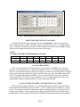
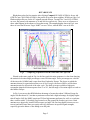
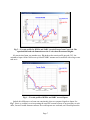
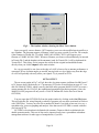
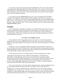
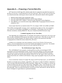
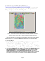
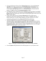
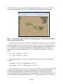
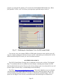
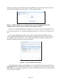
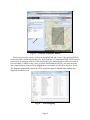
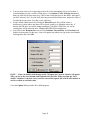
Operating Instructions for HFTA, Version 1.04
(HF Terrain Assessment for Windows)
February 22, 2013
This version of the HFTA Operating Instructions updates the method to download terrain data
files from the NED (National Elevation Database) USGS online servers. The MicroDEM program
then can be used to create terrain profiles for HFTA, using USGS map data in DEM (Digital
Elevation Model) or NED (National Elevation Database) seamless formats in the USA. In
addition, usage of SRTM (Shuttle Radar Topography Mission) 3-arc-second format is described,
allowing the user to generate terrain profiles for areas outside the USA. See Appendix A for
instructions on downloading and using digital terrain data.
PREFACE
HFTA is a ray-tracing program designed to evaluate the effect of foreground terrain on the
elevation pattern of up to four multi-element HF monoband Yagis in a stack. See Chapter 3 in the
21st Edition of The ARRL Antenna Book for details about the theory behind ray tracing and
diffraction in HFTA.
HFTA has a vastly improved operator interface compared to older DOS versions of its
predecessor programs, YT and YTAD. The program has been under continuous development since
1995. HFTA best models horizontally polarized Yagis, although a simple horizontal dipole model
has been added as well. HFTA takes into account the effects of Fresnel horizontal groundreflection coefficients, meaning that the ground conductivity and ground dielectric constant are
inputs to the program through the Options subscreen. (You will find that these ground coefficients
have only a minor effect on the elevation pattern at low angles, gradually becoming more
significant at higher elevation angles.) Besides reflection, HFTA also takes into account
diffraction. Please note: HFTA does not work with vertical polarization, only horizontal, and it
works best with directive arrays such as horizontally polarized Yagis or quads.
Fig 1 — HFTA main screen.
Page 1
HFTA’s output response is referenced to an isotropic radiator in free space; that is, in dBi. The
free-space gain assumed for the default four-element Yagi model is 8.5 dBi. Fig 1 shows HFTA’s
main window. We’ll get into details about operating HFTA later, but first we need to look at the
terrain data files you will need for your particular location.
Instructions for Running HFTA
Start up HFTA by clicking on its icon. Look again at Fig 1, which shows a typical main
window for HFTA. Like its stable mates TLW and YW, HFTA incorporates a number of “Tool
Tips.” When you move the mouse cursor and let it hover over a button or a text box on the screen,
a brief explanatory note will appear.
You can select up to four different terrain files, each with a set of heights for stacked antennas
and HFTA will overlay the resulting elevation patterns on a single high-resolution graph. I
regularly compare any patterns I generate to a reference 3-element Yagi over flat ground, usually
at a height of 60 feet on 21 or 28 MHz, or 100 feet for 14 or 7 MHz. (These are also the reference
antenna heights I specify when using the IONCAP or VOACAP propagation-prediction programs.)
HFTA saves the defaults you like to a startup file called YTW.DEF. If HFTA detects no
YTW.DEF file on bootup, it will automatically create a new one, showing blanks for the four
terrain files.
SELECTING A TERRAIN FILE
To select a Terrain File, click the left-mouse button with the mouse cursor in the appropriate
text box. A dialog box will open up asking you to “select existing terrain file” from a sorted list of
filenames. As usual in this familiar common-dialog style, you may change the subdirectory if you
have saved terrain filenames in other than the default subdirectory.
Keep in mind that you must have a terrain filename showing in the first position in HFTA, with
blanks in other positions if you like. Some operators like to keep FLAT.PRO in terrain filename 4
so they always have a reference flat terrain with which to compare the responses over actual
terrains. Click on the Cancel button to erase a filename in that Terrain Files box.
ANTENNA HEIGHTS
Once you’ve selected a terrain profile name, you will want to choose the type of antenna and
the number and heights of antennas in a stack. Click on the Ant. Type or Heights box you want.
A new dialog box will open. See Fig 2. The default when you first start HFTA is one 4-Ele. Yagi
antenna, at 100 feet in height. Let’s say that you want to specify three 4-Ele. Yagi antennas in a
stack at 90, 60 and 30 feet. You would place the cursor in the top left text box and edit the 100 to
be 90. Then you would edit the second box to be 60 and the third to be 30. You can move the
mouse or use the Tab key to advance the cursor from box to box. Once you click on OK, you
might want to set the same heights for the next Terrain Files box. The Copy buttons on the right
side of the Height 4 boxes give you a quick way of copying one row to another row. Click on the
Copy button you want and you will see the other two Copy buttons change their labels to “To”.
Click on the To button you want. By the way, always specify a height for each Terrain — 0 feet
won’t work right.
Page 2
Fig 2—Entering antenna types and heights for each terrain file.
SELECTING THE TYPE OF YAGI USED
Clicking on the button at the right down arrow in an Antenna box will open a drop-down
menu of antenna types available, including a dipole, and Yagis with as few as 2 elements all the
way to 8 elements. The gains in free space for these antennas are shown below in Table 1, along
with the boom lengths needed on 20 meters to achieve these gains.
Table 1
Free-Space Gain (dBi) and Boomlengths on 20 Meters
Antenna
Gain
20-m Boom
Dipole
2.15

2-Ele.
5.5
8'
3-Ele.
7.0
16'
4-Ele.
8.5
26'
5-Ele.
9.5
40'
6-Ele.
11.0
60'
8-Ele.
12.0
80'
OUT-OF-PHASE FEED
There is a useful feature in HFTA that earlier versions (such as YT) didn’t have. You may
choose to use out-of-phase drive to individual antennas in a stack. You do this by appending an
asterisk (*) to the end of a height number. For example, in a stack at 90, 60 and 30 feet, you might
run the top 90-foot high antenna out-of-phase with the two lower Yagis. Enter 90* in the top left
text box. Although employing out-of-phase drive is not often useful in terms of increasing the
overall performance of a stack of Yagis, sometimes it can cover high angles that a stack or any
single antenna cannot accomplish because of a steep mountainous terrain.
A CAVEAT ABOUT CLOSELY SPACED YAGIS IN A STACK
The internal Yagi model in HFTA is a very simple mathematical model. It does not compute
interactions between individual Yagis in a stack — HFTA assumes that each antenna is a “point
source.” For antennas stacked more than about a half wavelength apart this is not a problem. For
example, you should be cautious specifying spacings less than about 20 feet on 20 meters (and
proportionately scaled on other bands) because of mutual-coupling effects between real antennas.
Page 3
Spacings less about 20 feet on 20 meters will show a false increased gain in HFTA, even though
the real effects of interaction between the beams will actually be to decrease the gain.
SELECTING AN ELEVATION-STATISTICS FILE
Click in the box labeled Elevation File to select the nearest elevation-statistics file for your
targeted receiving area. See Fig 3. For example, from New England to Europe, choose
W1-MA-EU.PRN, standing for W1 (Massachusetts, the Boston area) to all of Europe. For each
amateur HF band from 80 to 10 meters, this file shows the percentage of time each elevation angle
is effective. These statistics were computed for all the times over the 11-year solar cycle when
each band is actually open. (If you run this example, you will find that the peak percentage for the
20-meter band is 12.7%, occurring at an elevation angle of 5 from Boston to all of Europe.)
Each elevation-angle statistic file is named in the generic format *.PRN and comes from the
CD-ROM shipped with the 19th through 21st editions of The ARRL Antenna Book (located in the
default HFTA subdirectory). The Antenna Book’s disk contains files for all regions of the USA to
Europe (EU), the Far East (JA), South America (SA), South Asia (AS), Southern Africa (AF), and
the South Pacific (OC), plus data files for a wide variety of other transmitting sites throughout the
world. You choose the general area where your transmitter is located during initial installation of
the HFTA program. Use the installation program for areas other than the ones you’ve already
installed. By the way, don’t try to select OUT.PRN as a statistical date file. It won’t work.
Fig 3 — Selecting Elevation-Statistical Files
CHANGING THE FREQUENCY
You can edit the frequency by clicking in the Frequency box on the main HFTA window. The
elevation-angle statistical data is automatically updated when you enter a different frequency.
Page 4
HFTA RESULTS
Fig 4 shows plots for four terrains after clicking Compute! BVCAPE-45.PRO is for my old
QTH on Cape Cod. K5MA-45.PRO is the profile of my next-door neighbor, K5MA on Cape Cod.
Both terrain profiles are for the 45 azimuth towards Europe. Terrain Files 3 and 4, FLAT.PRO,
are over flat ground, with antennas at 70 and 100 feet respectively. These serve as references to
show what happens in the absence of irregular terrain. The antenna heights shown in Fig 4 were
those of our actual 20-meter Yagis. N6BV’s was at 70 feet, while K5MA’s was at 80 feet.
Fig 4 — Comparing responses for K5MA and N6BV on Cape Cod.
Plotted on the same graph in Fig 4 as the line-graph elevation responses is a bar chart showing
the statistical elevation-angle percentages versus elevation angle. These percentages are valid for
all the times the 14-MHz band is open from New England to Europe. The degree to which the
antennas chosen for a particular terrain cover all these angles, the more effective will be those
antennas/terrain for all periods of the solar cycle. The ideal coverage would be a high-gain,
rectangular-shaped elevation response from 1 to 28, the full range of elevation angles covered on
this band to Europe.
In Fig 4 you can see that K5MA had an advantage of as much as about 5 dB into Europe for
angles less than about 10, but that my station next door had a slight advantage for slightly higher
takeoff angles. Still, the N6BV terrain and 70-foot high antenna performed as well, or even better
than, a station with a 70-foot high Yagi located over flat ground, the fourth (cyan) curve. Both
antennas were physically located 260 feet apart (we had a 260-foot long dipole between our two
towers) and into Europe there was rarely much of a difference in reported signal strengths,
especially given the nature of fast fading on an HF path.
Page 5
You can enlarge a portion of any HFTA graph using the mouse. For example, you might want
to expand the area from 2 to 15, where most of the action is occurring in Fig 4. Move the mouse
cursor to the upper left side of the portion you want to enlarge and hold down the left-mouse
button. While holding down the left-button, drag the cursor to the lower right and release the leftbutton. The graph will instantly blow up to show details in this region.
To return to the original graph, reverse the process—at the lower-right side of the graph, hold
down the left-button on the mouse and drag it upwards to the left. When you release the leftbutton the graph will return to its original area. Holding down the right-button on the mouse
allows you to scroll up and down on the graph. You can also choose to expand or contract the Xaxis for the graph by clicking on the appropriate Max. Elev. Angle option box on HFTA’s main
window. The default is 0 to 34. You may also choose to change the size of the graph by
dragging a corner or by clicking on the Maximize icon at the upper right.
If you want to read the exact value at some point on one of the curves, move the mouse cursor
to that point and a “Tool Tip” will appear, giving the angle, separated by the computed value at
that point. For example, moving the cursor to the top of the 4 bar-graph line in Fig 4 will show
“4 9.3”, meaning that at a 4 elevation angle the statistical percentage is 9.3% from New England
to Europe on 20 meters.
FIGURES OF MERIT
In Fig 4 you’ll see listed at the right-hand side a “Fig. of Merit” for each curve. This is a
weighted statistical average computed by multiplying the gain at each angle by the statistical
percentage that the band is open at that angle. The products for all the angles are averaged to
compute the Figure of Merit, which is calibrated in dBi.
For example, the flatland curve at 70 feet in Fig 4 has a Figure of Merit of 11.3 dBi, while the
curve for K5MA has a Figure of Merit of 11.9 dBi. This means that on average K5MA’s signal
will be 11.9 – 11.3 = 0.6 dB stronger than a flat-land station at 70 feet using the same Yagis.
I should caution you that a Figure of Merit (FOM) is only a “snapshot” of a complex situation.
You can easily find situations where the elevation response of an antenna over complex terrain is
better at low elevation angles than another antenna that has a higher FOM over the entire range of
possible elevation angles. Low angles are especially important during periods of low solar activity,
when the only possible modes of propagation are low-angle modes.
PLOTTING THE TERRAIN PROFILE
Clicking the Plot Terrain button with both K5MA-45.PRO and BVCAP45.PRO terrain files
selected yields the graph shown in Fig 5. K5MA’s tower was located behind his house on a rise
about 22 feet higher than my tower’s base. So his 80-foot high antenna was effectively 32 feet
higher than mine. This tended to give him an advantage at lower elevation angles, as might be
expected. In addition, there was a small peak almost equal in height to the N6BV antenna (the red
squashed diamond on the left-edge of the Y-axis). This peak tends to limit somewhat the elevation
response. Note that the Y-axis (maximum and minimum height) values on-screen are chosen
automatically in HFTA. Be careful when making assumptions about the steepness of a terrain!
Page 6
Fig 5 — Terrain profile for K5MA and N6BV towards Europe from Cape Cod. The
squashed blue and red diamonds near the Y-axis show the antenna heights.
My terrain into Japan was another story. Fig 6 shows the terrain profile towards 330, the
azimuth to Japan. About 300 feet away from the N6BV antenna was a small hill with a large water
tank on it.
Fig 6 — Terrain profile of K5MA and N6BV toward Japan.
Indeed, this difference was borne out consistently when we compared signals to Japan. See
Fig 7. Since we couldn’t co-exist operating the same DX contest because of our proximity to each
other, Jan and I would alternate contests: He would operate one weekend, and I would operate the
Page 7
next contest weekend. We ran a coax between our houses so that we could use each other’s
antennas. Even with an extra 400 feet of coax between the antennas, K5MA’s antenna/terrain was
always superior to my shot into Japan!
Fig 7 — Graph for K5MA and N6BV towards Japan from Cape Cod on 21.2 MHz.
DIFFERENT TYPES OF YAGIS
As mentioned earlier, you can select the type of antenna that HFTA uses for individual terrain
profiles. Fig 8 shows how different types of antennas affect the far-field elevation response at the
N6BV station in Windham, NH, in the direction of Europe for four different stacked antennas at
90/60/30 feet: a dipole, a 2-element Yagi, a 3-element Yagi and a 6-element Yagi.
Fig 8 — Response for 90/60/30’ stacks of different types of antennas.
Page 8
Options in HFTA
From HFTA’s main window, you can click on the Options button to bring up the Options,
HFTA form. Clicking OFF in the Diffraction box toggles the diffraction mechanism on and off,
to illustrate the effects of diffraction. When diffraction is off you will find that only a reflectionanalysis is run. In general, diffractions “fills in the holes” and “knocks down the peaks” in an
elevation pattern. This “fuzzing up” of the computed response is what happens in the real world,
where things are rarely very peaky or full of deep holes.
The drop-down box for Soil Conductivity (mS/m)/Dielectric allows you to choose the
conductivity and dielectric constant of the ground in the foreground of the antenna. A conductivity
of 5 mS/m and a dielectric constant of 13, typical of average to better-than-average ground, is the
default. You will find that changing the ground constants for a horizontally polarized antenna like
those used in HFTA changes the elevation pattern only a small amount, and only that at very high
elevation angles.
On this page you may select whether to display distances and elevations in feet or meters.
HFTA saves your choice of feet or meters in a definition file called YTW.DEF file so that you
don’t have to remember the next time it boots up. Along with the type of antenna mentioned
above, YTW.DEF also stores your preferred window sizes and locations for the elevation-response
and terrain-plot graphs.
If HFTA should crash somehow, you might end up with a corrupted YTW.DEF file. You
should navigate to the default HFTA subdirectory (usually located in the c:\AntBk20\HFTA
subdirectory if you did a standard installation) using Windows Explorer and delete the YTW.DEF
file there, or you can erase the YTW.DEF file using the Clear YTW.DEF button on the Options
page.
MOVING THE TOWER BACK
Several years ago, Zack, W1VT, a prominent VHF/UHF expeditioner who is fond of operating
from high mountain-top locations, told me he was concerned that his 6-meter antennas might be
too close to the edge of various drop offs to receive the benefit of ground reflections. On the
Options page of HFTA I have therefore added a function to evaluate the effect of moving the base
of a tower backward from the “zero” position stored in Terrain File 1. This “Move Tower”
function is most useful conceptually when the tower is placed at the edge of a steep drop off, but
you can also use it to move a terrain feature, such as a tall mountain peak, farther away from the
tower to see how the elevation response is affected.
See Fig 9. In the Options window, click on Move Tower. This will open a new window that
allows you to specify the distance to move back from the original tower position, either in feet or
meters. This will move the base back the specified distance, keeping the elevation the same as the
original tower elevation. In effect, this moves the tower back onto flat land, in the direction
directly behind the azimuth of interest. This is a common situation at the crest of a hill, where the
land is typically flat so that a house can be situated there.
Page 9
Fig 9 — The Options window, showing the Move Tower button.
Once you specify a move distance, HFTA requires you to save the modified terrain profile to a
new filename. The program suggests a filename, which you may override if you like. For example,
if the filename in Terrain File 1 is called “N6BV-045.00.PRO,” HFTA will suggest a new
filename of “N6BV-045.00-1.PRO.” Whatever filename you choose will automatically be inserted
in Terrain File 2 and the height(s) of the antenna(s) used for Terrain File 1 will be duplicated for
Terrain File 2. This allows you to compare the results for the original and modified terrains
directly when you click Compute! in the main window.
So, can you actually be too close to the edge of a cliff, at least as far as antenna performance is
concerned? If low elevation angles are needed, moving back on a level plain away from the edge
of a cliff will probably adversely affect your signals. Try it yourself in HFTA.
HFTA OUTPUT
The on-screen graphs in Fig 7 or Fig 8 show the elevation response (calibrated in dBi) from 1
to 34 degrees above the horizon, in ¼ increments. HFTA also writes this data in steps of 1 to a
disk file called OUT.PRN, which is used by the DOS utility program MAKEVOA.EXE to create a
custom antenna file for VOACAP, the sophisticated propagation-prediction program. (Note: the
MAKEVOA.EXE program will only create a VOACAP antenna file for the first set of data in
OUT.PRN.)
You may open the OUT.PRN file from the graph window by clicking on the Out File button.
This will open the file, using Notepad (or whatever program you may have associated in Windows
with *.PRN files). You may save the file to another file name if you wish to later use it in, say, a
spreadsheet for your own graphing and analysis. Note that a new OUT.PRN is created each time
you boot up HFTA.
OUT.PRN’s elevation data is delimited with commas. Character labels are delimited with
double quotation marks. This sort of data can be imported easily into a spreadsheet or database
management software for other types of manipulation, if you like.
Page 10
If you want to print the on-screen graphs click the Print button. The red trace will be printed
with a dotted line to help differentiate it on a black/white printer. The cyan trace will be printed
with a thinner line width to help differentiate it from the other traces. Note that if you try to print a
full-screen graphic, parts of it may be cut off towards the edges of the print. Resize the graphic to
print it fully on your particular printer.
You could also press the [Print Screen] key to put a copy of the graph onto the Windows
Clipboard. This can then be used by another Windows program, such as Word for Windows or
Paint Shop Pro. I find Paint Shop Pro to be particularly useful because by selecting Colors, Grey
Scale, I can view the graph as it would be printed on a black/white printer. To put a copy of only
the active window that has Windows “focus” onto the Clipboard, press the keyboard combination
[Alt][Print Screen] together.
Caveats
The HFTA program is still under development. For validation of its results, there are precious
little experimental data available showing careful measurements of HF elevation angles versus
terrain contours. Very few radio amateurs have access to a helicopter to really measure their
elevation patterns! HFTA does corroborate the results from a helicopter study done by WA3FET
and associates some years ago.
ACCURACY OF TERRAIN DATA
The terrain data itself from topographic maps can be “sparse” or somewhat questionable.
Irregularities that can be seen with the naked eye from the base of the tower are sometimes not
shown on a topo map, perhaps because a map was created years ago, before things were leveled by
bulldozers.
Furthermore, if you are using Shuttle Radar Topographic Mission (SRTM) terrain data you
have to recognize that a radar will see the tops of trees in a dense forest, not necessarily seeing the
underlying ground. And the area behind a steep peak will probably be partially blocked from sight
of the Space Shuttle-mounted synthetic-aperture radar.
The terrain model used by HFTA assumes that the terrain is represented by flat “plates”
connecting the elevation points in the *.PRO file with straight lines. The model is two
dimensional, meaning that range and elevation are the only data for a particular azimuth.
Obviously, the real world is three-dimensional. To get a true picture of the full effects of terrain, a
terrain model that shows azimuth along with range and elevation point-by-point would be
necessary. The computational requirements for such a fully 3-D model, even with the detailed
terrain data from MicroDEM, would be pretty horrendous.
You can get a feel for how your terrain affects signals launched in various azimuthal directions
by using separate data files for these directions. For example, from my old QTH in New
Hampshire, my coverage to central Europe goes from about 30 to 60. I have thus evaluated
azimuth shots for 5 increments: 30, 35, 40, 45, 50, 55 and 60. The overall effect for four
azimuths for a single antenna height can be plotted together on one screen to visualize the effect of
azimuth (and thus terrain shape). However, I will often plot the response of three real-world
Page 11
azimuths, plus a flat-ground case. This way I can judge what happens with changes in terrain
shape, compared to the result due only to the height over flat ground.
I had mentioned earlier that the internal mathematical model of an antenna is very simple and
does not take into account mutual impedances between antennas in a stack. There is another
simplifying assumption made inside HFTA — ray tracing is only done in the “forward” direction
from the tower towards the ionosphere on a single azimuthal heading. In earlier versions of this
program (YT and YTAD) I specifically limited the choices of antennas to directional antennas that
had little gain in the backwards direction. In HFTA I’ve included a simple dipole model so that
users can assess their own situations better. But the same program restrictions occur — ray tracing
is still only done in the forward direction, despite the fact that a dipole is bidirectional.
WHAT ABOUT DISTANT MOUNTAINS?
Some terrains may have tall mountain peaks that are further than 4400 meters from your tower
base. I normally recommend that you specify a distance of 4400 meters and a spacing of 30 meters
between distance samples in MicroDEM. HFTA can handle up to 149 data points (150 including
the tower base), so a typical PRO file will contain 149 points. You can manually edit a terrain file
to include a 5,000-meter peak at, say, 8000 meters away by deleting the last line in a file, and then
adding a line (using an ASCII word processor) saying: “8000 5000”.
ACCURACY AND TESTING THE RESULTS
What would I estimate as the “accuracy” of HFTA elevation predictions? I would say that I
would trust the results within plus/minus 3 dB. In other words, take HFTA results with a grain of
salt. Don’t obsess with changing the height of your antenna by fractions of a foot to see what
happens!
Having said that, now I must state that it is a good idea to compare elevation patterns in
intervals of perhaps 1 foot to assess whether HFTA is generating reasonably smooth results. Often,
the ¼ steps used in the program don’t align exactly and artificial spikes (or holes) can be created.
This is inherent in any ray-tracing program and can only be eliminated by using extremely small
angular step increments — and doing so would slow down execution even more.
After I do an evaluation for a particular antenna height, I will often specify an overlay of three
heights separated by one foot each. For example, if you are interested in a single antenna at a
height of 80 feet on 14.0 MHz for the K5MA-330.PRO terrain, you might first compare three
heights of 79, 80 and 81 feet, bracketing that height. The three curves overlaid on each other look
relatively smooth, except there is a 1.4-dB “bump” for the 79-foot height.
Now, run three heights of 80, 79 and 78 feet. Now, the curves for 78 and 79 feet look smooth,
but the 80-foot curve has a noticeable dip. This means that spurious artifacts of the ray-tracing
process are occurring at 80 feet in the program — but these would not occur in the real world. The
solution: don’t use the 80 foot point in the computer analysis, but you would mount your real
antenna at that 80-foot height if you like the response at 79 or 81 feet.
Page 12
FEEDBACK, PLEASE
I would greatly appreciate feedback from you about this program. If you have access to
validation data, I’d surely like to hear about it!
R. Dean Straw, N6BV
Senior Assistant Technical Editor (retired), ARRL
e-mail: [email protected]
Page 13
Appendix A — Preparing a Terrain Data File
HFTA needs an ASCII input file with the terrain data in a particular azimuthal direction from
the base of your tower. Terrain data may be in feet or in meters. There are four ways in which you
may obtain terrain data, and the pros/cons for each will be discussed in detail in this Appendix:
1.
2.
3.
4.
Manually from USGS paper topographic maps.
From the USGS DEM (Digital Elevation Model) maps database.
From the USGS NED “seamless” electronic maps (National Elevation Database).
From SRTM 3-arc-second electronic maps (Shuttle Radar Topography Mission) for areas
outside the USA.
Some sample data files are included with HFTA; for example, N6BV-45.00.PRO and N6BV330.00.PRO, meaning N6BV to Europe (at 45 azimuth) and to Japan (at 330). My old station
was located on a small hilltop in Windham, New Hampshire. These sample files have PRO
filename extensions, meaning PROFILE. They were created from DEM electronic maps.
Latitude/Longitude at Your Tower Base
One important piece of information you will need is the position of your tower. One way to get
this is to place a hand-held GPS receiver out at the base of your tower. Note that you may have to
smooth out the latitude/longitude GPS data by taking a number of measurements and then
averaging them to obtain an accurate location for your tower.
Another way to determine your tower position is to use Google Earth to find your street
address, zoom in and then home in on the exact latitude and longitude of your tower. You should
record the position of the base of your tower in your notebook for later use.
The Old-Fashioned, Paper-Map Way
The “old-fashioned” way to prepare a terrain profile was to buy an actual paper USGS
topographic map and painstakingly measure out the terrain data starting at a point representing
your own tower’s base, entering at each point along a desired azimuthal direction the distance
from the base and the elevation at that point into a disk file. For some parts of the world, where
digital terrain data isn’t available on the Internet, using a paper topographic map may be your only
choice.
If you examine the contents of a sample file using an ASCII word processor, you will find that
the data are arranged in two columns, separated by a tab, space or comma. Each line is terminated
with a carriage-return/linefeed and each line represents a single point. For example, to evaluate my
terrain towards Europe from my old location in New Hampshire, I drew a line from the base of my
tower at an azimuth of 45 towards the center of Europe. Where this line crossed each contour on
the topographic chart, I measured the distance from the tower base and entered it into the disk file.
Here is a sample of a typical data set I generated manually.
Page 14
feet
0
200
500
700
800
900
1000
1550
2200
4800
13200
430
420
410
400
380
360
340
360
340
340
360
The first data line starts at the base of the tower, at 0 feet distance. The elevation height above
mean sea level (also known as ASL, standing for Above Sea Level) at my old tower base was
430 feet. The next line in the data files shows that 200 feet from the tower base the elevation is
420 feet; at 500 feet the elevation is 410 feet, etc. I entered data at distances from the tower for
more than 13,000 feet (4000 meters), because even at that distance the effect is noticeable on
elevation pattern for low frequency antennas, like a 40-meter Yagi. HFTA will accept input of up
to 149 data points in an input terrain file, as mentioned before.
This method of producing terrain data manually is extremely labor-intensive. It was also hard
on the eyes, requiring a good magnifying glass and a steady hand with a set of calipers to measure
off the distance on the horizontal scale at the bottom of the paper map. For relatively
uncomplicated terrains (that is, ones not located in rugged mountains), I could complete a single
azimuth’s data profile in about a half hour. To show all azimuths of interest (“boxing the
compass,” as mariners are found of saying) takes a very long time!
TECHNOLOGY TO THE RESCUE — MICRODEM
Kevan Nason, NS4T, brought to my attention a really fine program that manipulates electronic
topographic data. The mapping program is called MicroDEM and a professor at the US Naval
Academy, Dr Peter Guth, is the author. Professor Guth and the US Naval Academy have
graciously allowed ARRL to put MicroDEM on the CD-ROM that accompanies this book.
MicroDEM automatically makes numerous terrain profiles, once you have downloaded the
appropriate electronic map files, described in detail later in this Appendix.
VERSIONS OF MICRODEM
The version (Alpha 7) of MicroDEM that is included presently on the CD-ROM that
accompanies this edition of The ARRL Antenna Book can create terrain profile files with USGS
DEM (Digital Elevation Model) and NED (National Elevation Dataset) data, but doesn’t work
with SRTM (Shuttle Radar Topographic Mission) terrain data. (See Appendix B for instructions
on setting up the Alpha 7 version.)
Dr Guth has modified versions of MicroDEM after June 6, 2009, to work correctly with SRTM
input. You will have to go to the MicroDEM website to download the complete basic package,
which is about 55 MB in size. After you have installed the basic version, you must then download
the latest executable Microdem.exe, following instructions also on the site. Later versions of
Page 15
MicroDEM will work with all DEM, NED and SRTM data sets.
http://www.usna.edu/Users/oceano/pguth/website/microdemdown.htm.
Once you have installed MicroDEM, bring it up on-screen. Fig A1 is a screen-shot of the
program with the Windham, NH quad map displayed, together with Tiger US Census data
showing roads, highways and streams. More on Tiger later.
Fig A1—Screen shot from MicroDEM program, showing Windham, NH, region.
SETTING OPTIONS IN THE LATEST MICRODEM FROM WEB SITE
If this is the first time you’ve used the MicroDEM program, you need to set some options to
generate data for HFTA. Click on the Options menu listing at the top of the main window.



Select the Units tab.
You probably will want to specify in the Lat/Long textbox the exact way you enter or show
latitude and longitude. For example, let’s say that your GPS shows your position at
42 4’ 30” N latitude and 82 7’ 35.1” W longitude. This is the so-called
“degrees/minutes/seconds” method of showing latitude or longitude. You would select the
“Decimal seconds” option. However, if your GPS showed the same position as 42.07500 N
and 82.12641 W, this is expressed in “Decimal degrees.” Click the OK button when finished.
Click on the Coordinates tab. In the Verify box, click on the option Keyboard entry. In the
Show roam on all maps box check the Reasonable option. Do this also for the Verify
Graphical Selections box. Click Keyboard selection for target run. The values for
latitude/longitude determined by double-clicking the mouse will now bring up a verification
box in which you can type the exact coordinates. Click the OK button when finished.
Page 16




Click on the Views tab and then click the Weapons Fans button. Click the LOS and fan
algorithm button. Make sure that the box labeled Radials from zoom map size is not
checked. Now, click Radial lines, discrete. Verify Ray Spacing is 5º (the default value).
Click Constant radial spacing and then verify Point Spacing (m) is 30 meters (also the
default). Click OK to return to the Fan Drawing Options window.
Set range rings to show constant-sized circles surrounding your tower location. I recommend
radii of 2200 and 4400 meters. First, check the box Draw range circles. Now click on the O
Range circles button and then type 2200 for the first range ring and 4400 for the second. Click
OK to exit this window.
Set the default subdirectories by clicking the Directories tab. MicroDEM creates a
subdirectory system where map data will be stored, usually in x:\Mapdata, where the “x”
denotes the disk drive you select during installation. The radial *.PRO files you will be
creating later will be stored in the x:\Mapdata\MD-PROJ\Fans subdirectory.
Generate a Weapons Fan to set additional default parameters. First, load the
“HangRockCanyon” sample DEM map using the File, Open, Open DEM menu selections.
Then click Calculate, Intervisibility, Viewshed. Move the cursor near to your location and
double-click the mouse. Type in the desired latitude and longitude and then click OK. A new
ViewShed Parameters window will open, as shown in Fig A2. Make sure you check Save
radials so that terrain profiles will be saved to disk.
Fig A2—Setting up ViewShed Parameters after double-clicking a location.

Close the Options dialog and then the MicroDEM program to save your options to disk.
Page 17
Getting Digital Map Data for the USA
As mentioned above, for the USA, the USGS (US Geologic Survey) maintains two types of
public-domain terrain data sets on the Internet. MicroDEM can use either of these data sets to
create terrain profiles for HFTA. There are advantages and disadvantages to each method:


DEMs (Digital Elevation Model) are essentially digital versions of the 7.5-minute quad paper
topographic maps with which most US hams (or hikers) are familiar.
NEDs (National Elevation Dataset) are “seamless” versions of the paper topographic maps.
USGS DEM MAPS
The DEM datasets are available from several commercial vendors. Some of these vendors
charge no fees for limited Internet access to the data. The NED datasets are available directly from
US Geological Survey, EROS Data Center, Sioux Falls, SD, on the Internet. I thank Pete Smith,
N4ZR, for giving me some vital tips on how to download and use NED files.
Downloading a specific DEM is usually faster than downloading a NED data file because the
DEM is generally smaller in size, by a factor of about two. However, you may need to merge as
many as four DEMs to cover an area large enough to create terrain profiles around a particular
tower location. Furthermore, finding the specific DEM(s) for a particular tower location can
involve quite a bit of hunting around at several Web sites, and you also must know the counties in
which various quads are located. In general, I recommend DEM files despite the merging
challenges, since the absolute accuracy of the DEM files appears to be better than of the
“smoothed” seamless NED files, especially on challenging terrain  such as on a mountaintop.
You need to know several simple facts before attempting to download DEM digital-terrain
data from the Web: the state and county, and possibly the ZIP Code too. It is very useful to have
an exact street address as well, which you can often find at http://www.qrz.com/. You will find
that it may not be immediately obvious what names the USGS (US Geologic Survey) has used to
label their quad 1:24000 topographic maps.
To see an overview map that shows the quad names near your location, go to the following
URL for MapMart: http://tinyurl.com/q8hleu. You will be presented with a map of the entire USA.
The easiest way to find an exact location is by specifying the street address by clicking in the
“Zoom to” drop-down box in the upper left-hand corner. See Fig A3. The red star was the location
of the N6BV mailbox at the front of the property when I lived in New Hampshire.
You will need to “Zoom Out” to see the names of the quad topo maps surrounding your target
location. Place the cursor on the red arrow when zooming out. Write down the quad names
surrounding your location. If your location is near the edge of a quad map (as many locations are),
you will need to download not only the quad map for your location, but also other nearby quads.
You may find it necessary to download and “merge” as many as four different quads to cover a
given location if it is located in the corner of its main quad map. For my old location in Windham,
Page 18
NH, I found it necessary to download the Derry quad in addition to the Windham quad and merge
the two.
Fig A3 – Result of zooming out four levels after searching for the exact street address at
N6BV’s old QTH in Windham, NH. The red star shows the N6BV location, bounded by topo
maps labeled Windham, Derry, Salem Depot and Sandown. Note checkbox “Display
Coordinates” at lower left that allows you to display latitude/longitude at the cursor, if you
wish.
Download DEMs
Go to this URL to download the DEMs: http://data.geocomm.com/dem/demdownload.html.
You must register once for free downloading of DEMs on this site. On the USA map shown in
Fig A4, click on your state and select your county. Click on the link Digital Elevation Models
(DEM) - 24K. (The label “24K” refers to the fact that this topo map has a scale of 24,000:1.)
Now, select the name of the quad you want to download and click the green Download button for
that quad.
Fig A4—USGS map selector screen. Click on your state.
Page 19
You will be presented with a link to click on, with a label similar to this:
1667372.DEM.SDTS.TAR.GZ (30 meter). When saving the map to disk, I usually edit this
confusing numerical name to something I can relate to, such as Windham_NH.SDTS.TAR.GZ to
describe my old location in New Hampshire. Note that you might have a choice of data in
increments of either 10 or 30 meters. Choose the 30-meter data, since the degree of precision in
the 10-meter data is not warranted for HF work and because 10-meter DEM files take far longer to
download. If there is no choice other than 10-meter data (as may happen for newer data sets),
MicroDEM can still automatically create 30-meter terrain profile information for HFTA to use.
Merging Topographic Maps
As mentioned above, at my old location in Windham, NH, I needed to merge two DEM maps,
because my tower was located near the junction of two topographic maps. In MicroDEM, first
make sure that you close any open DEMs.


Click on File in the top menu and then click on Data Manipulation, followed by Merge and
then DEMs. Click on Dems—pick single and you will be presented with a list of the DEMs
located in your default maps subdirectory. Select the first DEM you want, followed by the
second one you wish to merge. In my case, I selected the Windham, NH, and then the Derry,
NH, quads.
Then click Cancel to end the merging operation, and save the resulting merged file, using an
appropriate filename, such as “Merged Windham_Derry.DEM” or perhaps “N6BV.DEM.”
Finally, close the merge operation by clicking on File and then Close.
Merging 10-m and 30-m DEMs
Most USGS DEMs are 30-meter DEMs, meaning that the internal data is sampled at 30-meter
horizontal intervals. Some of the newer DEMs, however, are sampled at 10-meter intervals.
MicroDEM won’t allow you to merge these two different types directly. There is a workaround,
involving creating intermediate merged data files using the DTED format. At this point, however,
you may well want to consider downloading a NED data file rather than working with multiple
DEMs with different resolutions. However, if you choose to stick with DEMs, here’s the method
to merge, say, two 30-m DEMs and a 10-m DEM.





With no map showing on-screen, click on File in the top menu and then click on Data
Manipulation, followed by Merge and then DEMs and Dems—pick single.
Select the first 30-m DEM filename, followed by the second one. Click Cancel to end the
merge operation. Name the resulting file a temporary filename, say, “Merged.DEM” and get
back to the main screen by closing the dialog boxes and the map.
Now, you need to convert the merged 30-m DEM and the 10-m DEM to DTED files. Click on
File in the top menu, followed by Open, Open DEM and select the new “Merged.DEM” file.
Click File in the top menu, followed by Save DEM and then select the DTED format. Make
sure that the “Lat spacing (seconds)” and “Long spacing (seconds)” are set to “3”. Click on
OK and save to “Merged.DT1”. Again, get back to the main screen by closing the dialog
boxes and the map.
Click on File in the top menu, followed by Open, Open DEM and select the 10-m DEM file.
Click File in the top menu, followed by Save DEM and then DTED. Make sure that the “Lat
Page 20


spacing (seconds)” and “Long spacing (seconds)” are set to “3” (for 0.3 seconds). Click on
OK and save this to a filename such as “10m.DT1”. Close the dialog boxes and the map.
Now, you will merge the two DTED files. Click on File in the top menu and then click on
Data Manipulation, followed by Merge and DEMs and then DEMs—pick single. It may be
useful to type “*.DT1” followed by [Enter] in the Filename box to bring up only the DT1 files
you have created.
Select first the merged 30-m file (“Merge.DT1”), followed by the 10-m file “10m.DT1”. Click
Cancel to exit the merge function and name the file something else, perhaps “N6BV-1.DEM”.
Now, wasn’t that fun? It sounds very complicated but luckily you won’t have to do this very
often. Again, however, downloading a NED file may be more efficient.
Merging Across Different UTM Zones
You may live near where two maps you’d like to merge are in different UTM (Universal
Transverse Mercator) zones. Because of distortions at the edge of any map, which after all is
converting a round world (the Earth) to a flat-map representation, MicroDEM will not allow you
to directly merge these two maps across UTM boundaries. You use the same basic procedure as
above, using DTEDs to merge DEMs with 10-m and 30-m spacings rather than trying to merge the
DEMs directly. For this example we’ll merge two DEMs called “Dem1.DEM” and “Dem2.DEM.”






First, convert each DEM to DTED format. From the top menu, click File, Open, Open DEM
and select “Dem1.DEM.”
Save it as a DTED file by clicking File in the top menu, followed by Save DEM and then
DTED. Make sure that the “Lat spacing (seconds)” and “Long spacing (seconds)” are set to
“3” (for 0.3 seconds). Click on OK and save this as “Dem1.DT1”. Close the dialog boxes and
the map.
Process the second file. On the top menu click File, Open, Open DEM and select
“Dem2.DEM.”
Click File in the top menu, followed by Save DEM and then DTED. Make sure that the “Lat
spacing (seconds)” and “Long spacing (seconds)” are set to “3” (for 0.3 seconds). Click on
OK and save this as “Dem2.DT1”. Close the dialog boxes and the map.
Now merge the two DTED files. Click on File in the top menu and then click Data
Manipulation, followed by Merge and DEMs and DEMs—pick single. Again, it may be
useful to type “*.DT1” followed by [Enter] in the Filename box to bring up only the DT1 files
you have created.
Select “Dem1.DT1,” followed by “Dem2.DT1”. Click on Cancel to exit the merge function
and name the file something else, again perhaps “N6BV-1.DEM”. Close the dialog boxes and
the map.
Again, luckily you won’t have to do this special merging procedure too often!
SEAMLESS NED MAPS
MicroDEM can also use a “seamless” NED file to create a custom-sized topographic map
centered on the latitude/longitude you specify for the tower’s base. The latest URL for the MRLC
seamless data site is: http://www.mrlc.gov/viewerjs/. The default setting for downloading data is
Page 21
1 NED, which is what we need in the USA. Fig A5 shows the page that comes up for USGS
Seamless Data Distribution. (Note: Be aware that USGS seems to change this page often.)
Fig A5 — Initial setup window for MRLC Seamless Data page. The Data dropdown menu
shows the Download Tool icon.
The next screen will be similar to that shown in Fig A6. For example, at K1EA’s location in
Western Massachusetts, his 15/20-meter tower is located at 42 30' 52.96" N latitude and 7133'
0.39" W longitude. You now have two choices for entering coordinates. The most labor-intensive
one will place the tower exactly in the middle of the resulting NED DEM. Convert these to
decimal degrees, remembering that minutes are 1/60 of a degree and seconds are 1/3600 of a
degree:
42 + 30/60 + 52.96/3600 = 42.51471
71 + 33/60 + 0.39/3600 = 71.55011.
Now, add and subtract 0.1 to the tower’s position to define the rectangle surrounding the
tower base:
Top latitude = 42.61471 Bottom latitude = 42.41471
Left longitude = 71.65011 Right longitude = 71.45011.
The second method is easier to do in your head, but will result in a slightly offset NED file, but
one that is still large enough to cover the area around your tower. Simply add and subtract
5 minutes to/from the latitude and longitude to set the borders. You can ignore the values for
seconds. Following the above example, at a tower position of 42 30' 52.96" N latitude and 71 33'
0.39" W longitude, simply make the top border 42º 35' N, the bottom border 42º 25' N, the right
Page 22
border 71º 28' W, and the left border 71º 38' W. See Fig A6, where the “Switch to Degrees,
Minutes, Seconds” selection has been clicked previously to get to this “Download Tool” form.
Note too that I checked the “1 inch” elevation data checkbox — they really mean “1 arc-second”
rather than “1 inch.”
Fig A6 — Specifying coordinates for NED download. Tower is at 42 30' 52.96" N latitude
and 71 33' 0.39" W longitude, with 5 minutes subtracted and added to give corner
boundaries for data selection box.
However you decide to calculate the borders, now click on Add Area and you will next be
asked whether you really want to go on. Click OK and you will next be presented with the
Summary Request Page. Click the Modify Data Request button and the screen shown in Fig A7
will appear. Scroll down the page and make sure the National Elevation Dataset (NED) 1 Arc
Second box is checked and that you select GeoTIFF (instead of ArcGRID) for the Data Format.
Scroll down to the bottom of the page and click on Save Changes & Return to Summary button.
Now you’re back at the previous screen, but with the required format of the download changed
and updated.
Now click the Download button and follow the instructions to save the zipped file to your
hard disk. You should write down the name of the zipped file and save it to the subdirectory where
you usually place your DEM files. For a standard MicroDEM installation, that will be in:
C:\MapData\DEMs.
We’re done with USGS, but the fun isn’t quite over yet, because if you run MicroDEM at this
point, click File and then Open, Open DEM and try to open the zip file you just created, you will
get an error. What you now need to do is to extract from the zip file (use WinZip or whatever
Page 23
program you want) the file with the “tif” extension into the MapData\DEM subdirectory. When
you open this *.tif file, voila! You’ll have your topo map, open and ready to work on.
Fig A7 — Modifying the “Data Request” for a GeoTIFF output format.
You can now save your seamless DEM as a DEM with a descriptive name (such as your call
sign, for example), and open it directly to be sure it’s OK. At this point you can delete the *.tif file
and the associated zip file, because you won’t need them anymore.
ANOTHER NED SOURCE
The USGS (United States Geologic Survey) maintains a web site they call the “The National
Map.” Terrain data at this site is available in several formats, including some limited GeoTIFF
data described in the last section. However, the web site changes quite a lot as they built it out, and
trying to figure out where they’ve stashed things can be frustrating.
The URL is http://viewer.nationalmap.gov/viewer/. Click on the light blue arrow icon labeled
“Download Data” at the upper right of the screen. A drop-down menu will appear and you will
click on the link at the bottom, labeled “Click here to download by coordinate input.” This will
open a box like Fig A7, but will only accommodate input in decimal degrees of latitude and
Page 24
longitude. As in the previous method for gathering NED data, specify the upper and lower limits
for latitude and longitude, plus and minus 0.1° of the station’s position.
Fig A7 — Input bounding box. Use decimal degrees to enter bounding latitudes and
longitudes; that is, plus or minus 0.1 degrees of the station’s position.
When you’ve finished defining the bounding box (be careful to specify West longitudes in the
US as negative numbers), click the Draw Area button and choose “Elevation” data from the next
list.
Now, click the Next button to bring up the “USGS Available Data for download” screen.
Check “National Elevation Dataset (1 arc second) Pre-packaged Float format,” otherwise known
as “GridFloat.” (Do not check the “1/3 arc second” format unless you want to download some
huge files with that unnecessary amount of resolution.)
Fig A8 — Choose GridFloat data format.
Click Next again to bring up your shopping “Cart” on the left side of the screen and click the
Checkout button. You will be asked to provide your e-mail address, twice, and then you can click
Place Order. You’ll be given instructions to open the e-mail that will be sent to you automatically
when your data is available.
Page 25
Fig A9 — Click the “Checkout” button.
When you receive the e-mail, click on the download link and “Save to” the specified ZIP file
to your usual MicroDEM map subdirectory. By default this is C:\MapData\DEMs. USGS chooses
a one-degree by one-degree block of data surrounding your station location, which can result in
files exceeding 43 MByte in size. Once you have downloaded the ZIP file, you must unzip the
data using a program such as WinZip. Fig 10 shows an example of a Windows Explorer screen.
The filename automatically chosen by USGS imbeds the upper left-hand corner latitude and
longitude coordinates in it.
Fig 10 — After unzipping.
Page 26
The first file in Fig 10, the one with the “flt” (float) extension, is the file you would open using
MicroDEM to bring up a map. The rest of the files in the example subdirectory are also needed by
MicroDEM. However, once you bring up a MicroDEM map, you can save it as a “MD DEM” file
and erase the float directory and files.
Page 27
Getting Digital Map Data Outside the USA
DOWNLOAD AN SRTM FILE
The US government has released digital terrain data that covers 80% of the world (between
60° N and 54° S latitudes). The survey data was generated during a NASA Space Shuttle mission
in February 2000, and is called SRTM (Shuttle Radar Topography Mission) data. Inside the
continental USA, parts of Alaska, Hawaii, Puerto Rico and certain US Territories in the Pacific,
SRTM data is available with a resolution of 1 arc-seconds (roughly 30 meters). Outside these
areas, the US government has restricted the resolution to 3 arc-seconds (roughly 90 meters). Still,
the SRTM digital data is easier to use to generate terrain profiles for HFTA than are any manual
mapping methods.
The easiest way to download 3 arc-second SRTM (Shuttle Radar Topography Mission) data
that covers most of the world is to go to the website for the CGIAR Consortium for Spatial
Information: http://srtm.csi.cgiar.org/SELECTION/inputCoord.asp.
You will see a worldwide map with clickable blocks covering areas for which you want to
download topographic data. For example, let’s download topo data for GM3SEK in southern
Scotland. His tower is located at 54 44.160’ N, 4 28.283’ W. See Fig A11.
 Make sure the checkbox labeled Geo Tiff at the lower left is checked.
 Click on the box for the lower part of the UK.
 Now, click on the button Click here to begin search.
 Next, you’ll see a page similar to the one shown in Fig A12, where the area chosen is
zoomed in at the right to show some more detail.
Fig A11 — Starting page for CGIAR-CSI repository for SRTM data.
Page 28
Fig A12 — Detailed view of area selected in Fig A11.



If this is the area you want, click on Data Download (FTP). Save the zipped file to disk,
probably to the c:\MapData\DEMs subdirectory if you did a standard MicroDEM
installation.
Use WinZip or the Microsoft Explorer program to extract the *.TIF file from the zipped
file. Since each block contains detailed data for 5 of latitude and 5 of longitude, each
*.TIF file will be about 70 MB in size.
Open MicroDEM and click on File, Open, Open DEM to select a map.
Page 29
Creating Azimuth Terrain Files for HFTA in MicroDEM
You’ve finally managed to generate a digital map using MicroDEM! Now, you’ll need your
tower’s exact latitude and longitude — which you’ve gotten from a GPS or from Google Earth.
What we want now is for MicroDEM to generate terrain profiles in 5 steps of azimuth, with a
radius of 4400 meters around your tower base. This represents enough distance for HFTA to create
accurate reflection and diffraction ray-tracings to compute the far-field elevation responses.
Presuming that you have a map on-screen that covers the desired area, now click on Calculate,
Intervisibility, Viewshed menu. (You can also click on the Weapons Fan icon on the top of the
map window for this, if this icon is showing at the top of the map.) Double-click anywhere on the
map and a data entry box will open, where you enter the exact latitude and longitude at your
tower. Once you have entered these numbers and have clicked OK, another form, Viewshed
Parameters will open. See Fig A13.
Fig A13 — Setting the ViewShed Parameters. Note the “Save Radials” checkbox toward the
bottom of the form. Make sure it is checked. The “Fan name” at top is the filename base
under which the azimuthal profiles will be saved.
In the text box at the top in Fig A13, you choose a name for MicroDEM to use for subsequent
map operations, perhaps “N6BV-1” for the first tower location at a particular site. The filename
you specify will be what HFTA will use. For example, if you specify “N6BV-1”, MicroDEM will
create 71 files at 5-degree intervals, labeled N6BV-1-0.00.PRO, N6BV-1-5.00.PRO, N6BV-110.00.PRO, … up to N6BV-1-355.00.PRO.
Writing to disk takes about 5 seconds on a 1 GHz Pentium 3 computer running Windows 2000
Professional. Note that MicroDEM places the *.PRO files in the subdirectory: x:\Mapdata\MDPROJ\FANS, where “x:” is the subdirectory you chose on the Options, Directories tab. You may
Page 30
want to move these files manually using Windows Explorer to another subdirectory of your choice
after you finish working with MicroDEM.
Click the Observer range (m) text box and verify that it is 4400 meters, the default. Set the
Right Boundary to 355 degrees. Make sure you have clicked the selection “Save radials” at the
bottom. Don’t worry about setting the Observer AGL (m) or Target AGL (m) values. They’re
set at default values of 18 m (60 foot tower) and 2 m (the height of a soldier). Click OK to finish
creating the profiles.
Page 31
Other MicroDEM Capabilities
BRING ON THE TIGER!
This next step is not totally necessary, but it significantly adds to the process if you can
visualize how your terrain relates to the roads and streets near your location. This is where the US
Census Bureau “Tiger” data comes into play. Go to the following URL:
http://www.census.gov/geo/www/fips/fips65/ and look up the 5-digit FIPS code for your county.
This file gives a list of the so-called “FIPS” numbers. These identify a Tiger file for a
particular county in a particular state. (By the way, the term “Tiger” stands for “Topologically
Integrated Geographic Encoding and Referencing,” just in case you were wondering.) In my case,
I wanted to download Tiger information for Windham, NH, where the FIPS number is 33 015.
When you have the code (you’ll only need to do this once), go to
http://www.census.gov/geo/www/tiger/tiger2006se/tgr2006se.html and find your state at the
bottom of the page. Click on it and download the appropriate numbered zip file. For my old QTH
in New Hampshire, I chose to download “tgr33015.zip” to my c:\mapdata\Tiger\NH subdirectory.
(Note that I used the “Create New Folder” to create the “NH” subdirectory from the basic tree
structure MicroDEM created when it was installed.) Do not try to change the name assigned to this
zipped file or MicroDEM will not be able to find and associate it with DEMs you display. The
internal zipped file structure creates a temporary directory with that number as a name.
Now, you can bring up the map and add Tiger data to it. Start MicroDEM and click on the
File, Open, Open DEM selections from the top menu. For example, I might click on my merged
file “N6BV-1.DEM.” Then I click on the map icon on the top of the merged map’s window — the
one that looks like a miniature map of the southeastern USA. I select the file “tgr33015.zip” in the
c:\mapdata\Tiger\NH subdirectory and then marvel at what happens.
SETTING THE REFLECTANCE PARAMETERS
MicroDEM defaults to a gray “reflectance” display for elevation. I like to tweak the settings
for this, by clicking at the top menu Modify, Reflectance. Sometimes I use a color display of
elevations, so I may select IHS elev, with a Vert Exag of 8. Again, Fig A1 shows the resulting
display for my merged map with Tiger overlay of roads in red and streams in blue.
Page 32
Appendix B — Using the Older Version of MicroDEM
SETTING OPTIONS IN THE VERSION OF MICRODEM INCLUDED ON CD-ROM
Obtaining a completely new version of MicroDEM involves downloading about 60 MB of data
on the Internet. Some of you are still using dialup service and thus may be limited to using the
version of MicroDEM originally included on the CD-ROM bundled with the 20th or 21st Editions
of The ARRL Antenna Book. This limits you to the use of DEM or NED USGS data for the USA.
Here is how to set up the options in MicroDEM, Version 7.0 Alpha, the version on The ARRL
Antenna Book CD-ROM. Click on the Options menu listing at the top of the main window.




Select the Units tab (you may have to use the horizontal scroll arrows at the top to see all the
possibilities for options).
You may want to respecify in the Lat/Long textbox the exact way to specify or show latitude
and longitude. For example, let’s say that your GPS shows your position at 42 4’ 30” N
latitude and 82 7’ 35.1” W longitude. This is the so-called “degrees/minutes/seconds” method
of showing latitude or longitude. You would select the “Decimal seconds” option. However, if
your GPS showed the same position as 42.07500 N and 82.12641 W, this is expressed in
“Decimal degrees.”
Click on the Coordinates tab. In the Verify box, click on the option Keyboard entry.
In the Show roam on all maps box click on the Reasonable option. Do this also for the
Verify Graphical Selections box. The values for latitude/longitude determined by the mouse
will now bring up a verification box in which you can type the exact coordinates.
Now, click on the Views tab and then uncheck the box labeled Missing values set to sea level.
Click the Weapons Fans button to open the Fan Drawing Options page. Specify Ray Spacing
of 5º and Point Spacing of 30 meters. Make sure you click on the Radial lines option in the
upper right-hand corner. See Fig B1.
Fig B1—Fan Drawing Options. Make sure you click the Radial lines selection.
Page 33



You may next want to set a range ring to show the circle surrounding your tower location. I
recommend that you use a radius of 4400 meters. Use Options, Views, O Range circles and
then type 4400 for the first range ring, 2200 for the second and zero for the others. Note that if
you have selected “feet” for your units, this entry must still be 4400 meters, despite the label of
feet that shows on-screen. Yes, this is a bit confusing.
Set the default subdirectories by clicking the Directories tab. MicroDEM creates a
subdirectory system where map data will be stored, usually in x:\Mapdata, where the “x”
denotes the disk drive you select during installation. The radial *.PRO files you will be
creating later will be stored in the x:\Mapdata\MD-PROJ\Fans subdirectory.
Next click on the Weapons fan icon (or click Calculate, Intervisibility, and Viewshed) and
double-click anywhere on the map. A box will appear into which you type in the exact latitude
and longitude, then click OK.
Fig B2 — After you double-click the map in the “Weapons fan” process, this box will appear
after you key in the exact latitude and longitude and click OK. Make sure that the “Save
radials” checkbox is checked. Once you have selected this option, MicroDEM will continue to
use Save radials as a default value.
Close the Options dialog and the MicroDEM program.
Page 34