Download PHOTOMOD VectOr USER MANUAL

Software
PHOTOMOD
Module
PHOTOMOD VectOr
USER
MANUAL
Racurs, Moscow, 2009
PHOTOMOD
CONTENTS
1.
Overview ........................................................................................................................ 7
1.1. What is VectOr.............................................................................................................. 7
1.2. Hardware and software requirements............................................................................ 7
1.3. General software structure ............................................................................................ 7
1.4. Data types...................................................................................................................... 8
1.4.1. Vector maps structure ................................................................................................ 8
1.4.1.1. Vector map sheet................................................................................................. 8
1.4.1.2. Map nomenclature – sheet title ........................................................................... 8
1.4.1.2.1. Nomenclature of topographic maps ................................................................ 8
1.4.1.2.2. Nomenclature of geographic maps ............................................................... 10
1.4.1.2.3. Nomenclature of aerial navigation maps ...................................................... 13
1.4.1.3. Work region ...................................................................................................... 13
1.4.1.4. Structure of vector user maps............................................................................ 14
1.4.1.5. Group objects .................................................................................................... 15
1.4.1.6. Graphic map object ........................................................................................... 15
1.4.2. Raster map structure ................................................................................................ 15
1.4.3. Matrix map structure................................................................................................ 16
1.5. Scale range .................................................................................................................. 16
1.6. VectOr installation ...................................................................................................... 16
2.
VectOr interface.......................................................................................................... 16
2.1. Basic info .................................................................................................................... 16
2.1.1. Start and exit ............................................................................................................ 16
2.1.2. Moving map image .................................................................................................. 17
2.1.3. Moving cursor.......................................................................................................... 17
2.1.4. Getting object description........................................................................................ 17
2.1.5. Hot keys ................................................................................................................... 18
2.2. “File” menu options .................................................................................................... 18
2.2.1. Creating digital map................................................................................................. 19
2.2.1.1. Creating new map ............................................................................................. 19
2.2.1.2. Creating plan ..................................................................................................... 19
2.2.1.3. Creating user map ............................................................................................. 20
2.2.1.4. Creating matrix.................................................................................................. 20
2.2.1.4.1. Fast mode of matrix creation ........................................................................ 20
2.2.2. Opening digital map................................................................................................. 21
2.2.3. Map tree ................................................................................................................... 21
2.2.4. Loading data from external formats......................................................................... 21
2.2.4.1. Loading vector data........................................................................................... 21
2.2.4.2. Loading raster data............................................................................................ 22
2.2.4.2.1. Loading BMP files ........................................................................................ 22
2.2.4.2.2. Loading PCX files......................................................................................... 22
2.2.4.2.3. Loading TIFF files ........................................................................................ 22
2.2.5. Saving data............................................................................................................... 22
2.2.5.1. Saving digital map............................................................................................. 22
2.2.5.2. Saving data in exchange format ........................................................................ 22
2.2.6. Map upgrading ......................................................................................................... 23
2.2.7. Printing a map .......................................................................................................... 23
2.3. “Edit” menu options .................................................................................................... 23
2.4. “View” menu options .................................................................................................. 24
2.4.1. View contents (Map structure) ................................................................................ 24
© 2009
2
VectOr
2.4.2. Map displaying mode (Map image)......................................................................... 25
2.4.3. Raster displaying parameters (Raster list) ............................................................... 25
2.4.4. Matrix displaying parameters (Matrix list).............................................................. 25
2.4.5. User map displaying parameters.............................................................................. 25
2.5. “Search” menu options................................................................................................ 25
2.5.1. Search and mark objects .......................................................................................... 26
2.5.2. Searching objects by query ...................................................................................... 26
2.5.3. Searching objects by selected area........................................................................... 27
2.5.4. Searching objects by name ...................................................................................... 27
2.6. “Tools” menu options ................................................................................................. 27
2.7. “Scale” menu options .................................................................................................. 28
2.8. “Options” menu options .............................................................................................. 28
2.8.1. Map palette .............................................................................................................. 29
2.8.2. Setting fonts ............................................................................................................. 29
2.8.3. Image size and scale ................................................................................................ 29
2.9. “Window” menu options............................................................................................. 29
2.10.
“Help” menu options ............................................................................................... 30
3.
Basic application tasks................................................................................................ 30
3.1. Editing passport of vector map ................................................................................... 30
3.2. Vector map editor........................................................................................................ 31
3.2.1. General information ................................................................................................. 32
3.2.1.1. General information related to object editing ................................................... 32
3.2.1.2. Map editor options ............................................................................................ 32
3.2.1.3. Object selection................................................................................................. 33
3.2.1.4. Unselecting objects ........................................................................................... 33
3.2.1.5. Selecting object part.......................................................................................... 33
3.2.1.6. Editing object part ............................................................................................. 33
3.2.1.7. Completing operation........................................................................................ 33
3.2.1.8. Canceling operation .......................................................................................... 33
3.2.1.9. One step Undo................................................................................................... 34
3.2.2. Object creation......................................................................................................... 34
3.2.2.1. Object creation modes....................................................................................... 34
3.2.2.2. Creation of map object ...................................................................................... 34
3.2.2.3. Point object creation.......................................................................................... 34
3.2.2.4. Line object creation........................................................................................... 34
3.2.2.5. Polygon object creation..................................................................................... 35
3.2.2.6. Creating object with the code of existing object............................................... 35
3.2.2.7. Creating object group by coordinates, retrieved from file ................................ 36
3.2.2.8. Creating subobject............................................................................................. 37
3.2.2.9. Creating vector object from conditional object................................................. 37
3.2.2.10. Supplementary modes of object creation......................................................... 37
3.2.2.11. Map legend ...................................................................................................... 38
3.2.3. Deleting objects ....................................................................................................... 38
3.2.3.1. Deleting selected object .................................................................................... 38
3.2.3.2. “Delete” panel ................................................................................................... 38
3.2.3.3. Deleting one subobject...................................................................................... 38
3.2.3.4. Deleting all subobjects ...................................................................................... 38
3.2.4. Map objects editing.................................................................................................. 38
3.2.4.1. Changing code of marked objects ..................................................................... 38
3.2.4.2. Copying object to user map............................................................................... 38
3.2.4.3. Copying all subobjects ...................................................................................... 38
3
RACURS Co., Ul. Yaroslavskaya, 13-A, office 15, 129366, Moscow, Russia
PHOTOMOD
3.2.4.4. Full copy of object ............................................................................................ 39
3.2.4.5. Moving object ................................................................................................... 39
3.2.4.6. Changing object type......................................................................................... 39
3.2.4.7. Expanding vector line ....................................................................................... 39
3.2.4.8. Marking (grouping)........................................................................................... 39
3.2.4.9. Viewing map control information ..................................................................... 39
3.2.4.10. Changing scale range of marked objects ......................................................... 39
3.2.4.11. “Mark” panel.................................................................................................... 39
3.2.4.11.1. Restoring previously deleted objects .......................................................... 39
3.2.4.11.2. Intersection of marked objects .................................................................... 39
3.2.4.11.3. Smoothing marked objects.......................................................................... 39
3.2.4.11.4. Filtering marked objects ............................................................................. 39
3.2.4.11.5. Copying marked objects to user map.......................................................... 40
3.2.4.11.6. Deleting marked objects ............................................................................. 40
3.2.4.12. “Text” panel..................................................................................................... 40
3.2.4.13. “Group” panel .................................................................................................. 40
3.2.4.14. “Topology” panel............................................................................................. 40
3.2.4.14.1. Merging objects .......................................................................................... 40
3.2.4.14.2. Copying object part..................................................................................... 40
3.2.4.14.3. Creating subobject by existing object ......................................................... 41
3.2.4.14.4. Creating object intersections....................................................................... 41
3.2.4.14.5. Dissection of line object.............................................................................. 41
3.2.4.14.6. Dissection of polygon object ...................................................................... 41
3.2.4.14.7. Joining object vertices................................................................................. 41
3.2.4.14.8. Joining line objects ..................................................................................... 41
3.2.4.14.9. Creating a node ........................................................................................... 41
3.2.4.14.10. Smoothing object ...................................................................................... 41
3.2.4.14.11. Filtering objects ........................................................................................ 41
3.2.4.14.12. Joining objects .......................................................................................... 41
3.2.4.15. Restoring edited objects................................................................................... 42
3.2.5. Processing semantics of marked objects.................................................................. 42
3.2.5.1. Adding semantics .............................................................................................. 42
3.2.5.2. Deleting semantics ............................................................................................ 42
3.2.5.3. Replacing semantics.......................................................................................... 42
3.2.6. Vertex operations..................................................................................................... 42
3.2.6.1. Editing marked vertex ....................................................................................... 43
3.2.6.2. Editing common vertices of adjacent objects.................................................... 43
3.2.6.3. Deleting vertex .................................................................................................. 43
3.2.6.4. Adding vertex.................................................................................................... 43
3.2.6.5. Closing object.................................................................................................... 43
3.2.6.6. Object rotating................................................................................................... 43
3.2.6.7. Renumbering vertices........................................................................................ 43
3.2.7. Labels on the digital map......................................................................................... 43
3.2.7.1. Creating labels................................................................................................... 43
3.2.7.2. Editing labels..................................................................................................... 43
3.3. Data sorting(compression) .......................................................................................... 43
3.4. Measurements on a map.............................................................................................. 44
3.4.1. Length of drawn line................................................................................................ 44
3.4.2. Object length............................................................................................................ 44
3.4.3. Length of segment.................................................................................................... 44
3.4.4. Area of drawn polygon ............................................................................................ 44
3.4.5. Object area ............................................................................................................... 44
© 2009
4
VectOr
3.4.6. Coordinates calculations .......................................................................................... 45
3.4.7. Distance from point to object................................................................................... 45
3.4.8. Distance between map objects ................................................................................. 45
3.4.9. Building buffer zone ................................................................................................ 45
3.4.10. Crossing marked objects....................................................................................... 45
3.4.11. Intersection of marked and selected objects......................................................... 46
3.4.12. Defining map “empty” spaces (no object areas) .................................................. 46
3.4.13. Marked objects operations.................................................................................... 46
3.4.14. Objects statistical info .......................................................................................... 46
3.4.15. Marked objects statistical info.............................................................................. 46
3.4.16. Building loxodrome.............................................................................................. 46
3.4.17. Building orthodrome ............................................................................................ 46
3.4.18. “Matrix” panel ...................................................................................................... 46
3.4.19. Calculating absolute elevation.............................................................................. 47
3.4.20. Building profile along drawn line......................................................................... 47
3.4.21. Building profile along existing object .................................................................. 47
3.4.22. Building viewshed ................................................................................................ 47
3.4.23. Building buffer zones ........................................................................................... 48
3.4.24. 3D terrain displaying ............................................................................................ 48
3.4.25. Results displaying................................................................................................. 48
3.5. Editing classifier.......................................................................................................... 48
3.5.1. Creating and editing classifier ................................................................................. 48
3.5.2. Editing classifier objects.......................................................................................... 50
3.5.2.1. New object creation........................................................................................... 51
3.5.2.2. Copying object .................................................................................................. 51
3.5.2.3. Copying group of objects .................................................................................. 52
3.5.2.4. Deleting object .................................................................................................. 52
3.5.2.5. Deleting object group........................................................................................ 52
3.5.2.6. Filtering classifier objects ................................................................................. 52
3.5.2.7. Searching for classifier objects ......................................................................... 52
3.5.2.8. Displaying style of classifier object .................................................................. 52
3.5.2.9. Semantics of classifier objects .......................................................................... 52
3.5.2.10. Scale range of classifier objects....................................................................... 52
3.5.2.11. Printing style of classifier objects.................................................................... 53
3.5.3. Editing general classifier data.................................................................................. 53
3.5.4. Layers editing .......................................................................................................... 53
3.5.5. Semantics editing ..................................................................................................... 54
4.
Linked application tasks............................................................................................. 54
4.1. General information .................................................................................................... 54
4.2. Loading matrix map from GRD format ...................................................................... 55
4.3. Combining Work region to one map sheet.................................................................. 56
4.3.1. Removing borders of source map sheets ................................................................. 56
4.3.2. Creating border of output region ............................................................................. 56
4.4. Vector map transformation ......................................................................................... 56
4.4.1. Map transformation to control coordinates by map border ..................................... 57
4.4.2. Map transformation to control coordinates by map corners .................................... 57
4.4.3. Map transformation using control points by map border ........................................ 57
4.4.4. Map transformation using control points by map border ........................................ 57
4.4.5. Map transformation to selected zone of Gauss-Kruger coordinate system ............. 57
4.4.6. Map transformation to conic conformal projection for the block Europe ............... 57
4.4.7. Map transformation to conic conformal projection for the block Asia ................... 57
5
RACURS Co., Ul. Yaroslavskaya, 13-A, office 15, 129366, Moscow, Russia
PHOTOMOD
4.4.8. Map transformation to conic conformal projection for 1:4 000 000 map (Russia) . 57
4.4.9. Map transformation to Transverse Mercator projection .......................................... 58
4.4.10. Map transformation to cylindrical projection for Russia’s latitudes.................... 58
4.5. Joining sheets of Work region..................................................................................... 58
4.5.1. Control of joining objects on the sheet borders in the Work region........................ 58
4.5.2. Remove border “undershoots”................................................................................. 58
4.5.3. Automatic combining joined objects to a group...................................................... 58
4.6. Vector map georeferencing ......................................................................................... 58
4.6.1. Creating catalog of control points............................................................................ 59
4.6.2. Running process....................................................................................................... 59
4.6.2.1. Preparation ........................................................................................................ 59
4.6.2.2. Control points rejection..................................................................................... 60
4.6.2.3. Error messages and warnings............................................................................ 60
4.7. Raster image transformation ....................................................................................... 60
4.7.1. Raster transformation, step by step.......................................................................... 61
4.8. Export to DXF format ................................................................................................. 62
4.8.1. Symbol file structure................................................................................................ 62
4.8.1.1. Sample of symbol file ....................................................................................... 63
4.8.2. Creation of symbol file (DXL) ................................................................................ 63
4.8.2.1. Assigning semantics.......................................................................................... 64
4.9. Control of absolute elevations..................................................................................... 64
5.
Useful advises............................................................................................................... 65
5.1. Creation of arbitrary map fragment............................................................................. 65
5.2. Creating raster map by paper source........................................................................... 65
6.
Appendix А. DIR file structure.................................................................................. 66
7.
Appendix B. Sample of SXF file ................................................................................ 66
8.
Appendix C. MTRCREA.TXT file structure ........................................................... 69
© 2009
6
VectOr
1.
Overview
1.1.
What is VectOr
The VectOr software is a powerful desktop cartography and GIS system, developed for
digital maps creating, editing and printing out. You can create digital map based on separate
digital map sheets of different scales, types and nomenclatures. VectOr aggregates
complete list of tools for visualization, creating, editing and searching map objects. You can
add different types of objects including non-cartographic ones to the map, display fragments
of the map, using different scales, select objects and process groups of objects based on
semantics and metrics parameters.
VectOr is running under Windows 95 or Windows NT operation systems.
VectOr supports MDI interface and drag and drop mode to make the system user-friendly
and simple. You can use True Type fonts while map creation and make high quality
hardcopies, using a comprehensive list of output devices, supported by MS Windows.
The system kernel is implemented as a set of Dynamic Loading Libraries (DLLs) that allows
to add any map-handling functions easily. Applications can be created using different C++
compilers as well as MS Visual Basic and databases such as FoxPro or Paradox.
The main features of VectOr system are as follows:
•
creation and using hierarchical structure of database, including following levels:
work region, map sheets, layer, objects;
•
editing digital maps using GUI: creating new level, updating, deleting, copying
and restoring map objects
•
displaying map objects, using standard geographic, topographic, cadastral and
other map symbols
•
supporting standard Russian map classifiers (object coding)
•
supporting user-created map symbols
•
measurements on the map: distances, areas, perimeters, buffer zones, statistical
parameters
•
colorful and grayscale hardcopies, changing map contents and scale when output
•
WYSIWYG mode;
•
C++, C, Pascal, Delphi, Visual Basic, Builder C++ and other programming
interfaces.
1.2.
•
•
•
Hardware and software requirements
Pentium;
16 mb RAM;
Windows 95,98,2000,NT.
1.3.
General software structure
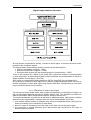
VectOr is implemented as module-separated multitasking system. All modules may be called
from the main shell. VectOr includes:
•
digital maps manager;
•
command shell;
•
service modules.
VECTOR.EXE file is used as a command shell. It is responsible for user-interface. Digital
maps manager is a DLL used for digital maps creating, editing, etc. Service modules are
data converters, printing modules, modules of calculations and analysis and others. All of
them are also implemented as DLLs.
Such a structure allows users to create their own applications and easily integrate them to
the system.
See also \DOC\MAPAPI.DOC file.
7
RACURS Co., Ul. Yaroslavskaya, 13-A, office 15, 129366, Moscow, Russia
PHOTOMOD
1.4.
Data types
The digital map may contain following cartographic datasets:
• vector maps,
• raster images,
• matrix datasets
Different types of datasets can be processed separately or as a whole. They can be
converted to a number of formats or from one type to another, displayed, printed out, edited,
etc.
1.4.1. Vector maps structure
VectOr processes vector maps, stored in open SXF format. Datasets from F1, F20V, MIF /
MID, DXF and other vector formats can be converted to/from SXF.
For SXF description see \DOC\SXF3-30.TXT и DOC\SXF4TXT.DOC files.
1.4.1.1.Vector map sheet
Digital vector map dataset includes:
• Passport data corresponding to map sheet (nomenclature, scale, projection,
coordinate system, rectangular and geodetic coordinates of corners etc);
• Metrics data(coordinates of vector elements);
• Object attributes (semantics data)
Object of a digital map is a collection of digital data (metrics, semantics, reference data)
corresponding to real world object (bridge, river, etc.) or a group of real world objects (block
of buildings) or a part of object if it is a complex one (some part of a building).
Vector objects can be separated to different layers on the map based on their thematic
properties (rivers, roads, etc). According to thematic layer each vector object can be
represented by symbol or pattern included to the map legend. These symbols (patterns) are
stored in the digital map classifier.
Following are the limitations of VectOr digital map:
• up to 65536 types of objects
• up to 255 layers
• up to 65536 types of characteristics for each type of objects
Standard topographic digital map uses about 2000 types of objects, 16 layers and 200
characteristics.
1.4.1.2. Map nomenclature – sheet title
To make it easier and faster to look for map sheets of different scales and ground location,
every map sheet is assigned unique name, called Nomenclature. Nomenclature (map sheet
title) is placed on the top (north) part of sheet either in the middle or right side. Usually
Nomenclature is following by a name of largest town located on the map.
Structure of Nomenclatures depends on map type (topographic, geographic, aerial
navigation, city plans, etc), scale and coordinate system.
Russian Nomenclature structure based on 1:1 000 000 map sheets. Any of them covers
ground area of 6 degrees of longitude and 4 degrees of latitude. Nomenclature of
1:1 000 000 map sheet includes number of “Latitude zone” (Latin capital character starting
from equator (A-zone) to the north) and number of “Longitude zone” (integer number starting
from 180 degrees longitude (0-zone) to the east). Thus, for example 1:1 000 000 map sheet
of area around city of Smolensk is named N-36 (Smolensk).
1.4.1.2.1. Nomenclature of topographic maps
Nomenclature (map sheet title) of topographic maps depends on their scales. There is a list
of standard scales of topographic maps below:
- 1: 1 000 000,
© 2009
8
VectOr
- 1: 500 000,
- 1: 200 000,
- 1: 100 000,
- 1: 50 000,
- 1: 25 000,
- 1: 10 000.
- 1: 5 000.
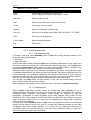
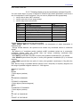
Template of Nomenclature of 1:10 000 map looks like:
9. Z - 99 - 999 - 9 - 9 - 9. Z
1 2 34 567 8 9 10 11
Dot or dash may be used as delimiter.
Character number
Meaning
1
Hemisphere (0 - north, 1 - south)
2
“Latitude zone” (Latin character from A to U). Numbering is
starting from equator
3, 4
“Longitude zone” (Integer from 1 to 60). Numbering is starting
from meridian of 180 degrees to the east
5, 6, 7
Number of 1:100 000 map sheet (1-144) or number of 1:200 000
map sheet (1-36) or number of 1:500 000 map sheet (1-4)
8
Number of 1:50 000 map sheet (1-4) on 1:100 000 map sheet
9
Number of 1:25 000 map sheet (1-4) on 1:50 000 map sheet
10
Number of 1:10 000 map sheet (1-4) on 1:25 000 map sheet
11
Sheet type (Latin characters A - D) can be one of following:
• single (A, B, C, D)
• double (A, C)
• four sheets in one (A)
Sheet type depends on latitude zones:
• zones A - O – single sheet
• zones P - S – double sheets
• zones T - U – sheets “four in one”
Characters 8, 9, 10 depending on sheet type assigned following values:
• 1,2,3,4
if single sheet
• 1,3
if double sheet
• 1
if “four in one” sheet
Character 8 is optional
Samples of nomenclatures:
Scale 1: 1 000 000:
0. A-01,
0. A-60
Scale 1: 500 000:
0. A-01-001,
0. A-01-004,
1. A-60-001,
1. A-60-004
Scale 1: 200 000:
0. A-01-001,
0. A-01-036,
1. A-60-001,
1. A-60-036
Scale 1: 100 000:
0. A-01-001,
0. A-01-144,
1. A-60-001,
1. A-60-144
Scale 1: 50 000:
0. A-01-001-1,
9
RACURS Co., Ul. Yaroslavskaya, 13-A, office 15, 129366, Moscow, Russia
PHOTOMOD
0. P-01-144-3,
0. T-60-144-1,
1. A-60-144-2
Scale 1: 25 000:
0. A-01-001-1-1,
0. A-01-144-1-4,
0. A-60-144-4-1,
0. A-60-144-4-3
Scale 1: 10 000:
0. A-60-001-1-1-1
0. A-60-001-1-2-3
0. A-60-144-4-1-1
0. A-60-144-4-3-1
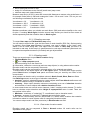
The template of Nomenclature of 1:5 000 map sheet looks like:
9. Z - 99 - 999 - 999
1 2 34 567 89 10
The symbols 1,2,3,4,5,6,7 correspond to 1:100 000 map sheet.
Symbols 8,9,10 (integers 1 - 256) - number of 1:5 000 map sheet on 1:100 000 map sheet.
Sample of 1:5 000 nomenclature: 0. A-60-144-256.
1.4.1.2.2. Nomenclature of geographic maps
Standard scale range for geographic maps includes following scale values: 1 : 500 000,
1 : 1 000 000, 1 : 2 500 000, 1 : 5 000 000, 1 : 10 000 000.
Geographic maps are created in 4 subsystems (zones) that cover the entire globe.
• Midlatitude (main) in conformal conic projection (standard parallels are 30 and 60
degrees (north))
• North (polar) - central meridians are 90 degrees (east and west). Conformal
azimuthal (stereographic) projection (standard parallel is 60 degrees (north)).
• South (polar) - central meridians are 90 degrees (east and west). Conformal
azimuthal (stereographic) projection (standard parallel is 60 degrees (south)).
• Equatorial - conformal cylindrical Mercator projection (standard parallels are 26 deg
08.4 min south and north).
Midlatitude subsystem used for mapping of north hemisphere in 1:500 000 - 1:10 000 000
scale range. Subsystem includes following 5 blocks:
• Europe (central meridian is 20 deg east), code 1
• Asia (central meridian is 90 deg east), code 2
• Pacific ocean (central meridian is 170 deg west), code 3
• North America (central meridian is 40 deg west), code 4
• Atlantic ocean (central meridian is 40 deg west), code 5
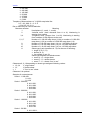
Blocks of midlatidude subsystem are composed as follows.
Europe, Asia, North America, Atlantic Ocean
10
11
00
01
Pacific ocean
© 2009
10
VectOr
00
01
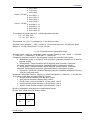
Composing polar subsystems
20
21
22
10
11
12
00
01
02
Composing equatorial subsystem
20
21
22
23
24
10
11
12
13
14
00
01
02
03
04
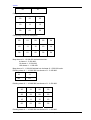
Map sheet of 1 : 10 000 000 scale divided into:
4 sheets 1 : 5 000 000;
16 sheets 1 : 2 500 000;
100 sheets 1 : 1 000 000.
Map sheet of 1 : 1 000 000 divided into 4 sheets of 1: 500 000 scale.
Dividing sheet of 1 : 10 000 000 into sheets of 1 : 5 000 000.
10
11
00
01
Dividing sheet of 1 : 10 000 000 into sheets of 1 : 2 500 000.
30
31
32
33
20
21
22
23
10
11
12
13
00
01
02
03
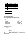
Dividing sheet of 1 : 10 000 000 into sheets of 1 : 1 000 000.
11
RACURS Co., Ul. Yaroslavskaya, 13-A, office 15, 129366, Moscow, Russia
PHOTOMOD
90
80
70
60
50
40
30
20
10
00
91
81
71
61
51
41
31
21
11
01
92
82
72
62
52
42
32
22
12
02
93
83
73
63
53
43
33
23
13
03
94
84
74
64
54
44
34
24
14
04
95
85
75
65
55
45
35
25
15
05
96
86
76
66
56
46
36
26
16
06
97
87
77
67
57
47
37
27
17
07
98
88
78
68
58
48
38
28
18
08
99
89
79
69
59
49
39
29
19
09
Dividing sheet of 1 : 1 000 000 into sheets of 1: 500 000.
10
11
00
01
Standard nomenclature of geographic map includes subsystem code or Midlatitude block
code, scale code and sheet number.
Codes of subsystems, Midlatitude blocks and scales are as follows:
Subsystem (block) name
Subsystem code Scale
1:10 000 000
Blocks
of
a
Midlatitude
1: 5 000 000
1
subsystem:
2
Europe
1: 2 500 000
3
Asia
1: 1 000 000
4
Pacific ocean
1: 500 000
5
North America
For the summary
6
Atlantic ocean
enlarged sheets
North pole subsystem
1:10 000 000
7
South pole subsystem
1: 5 000 000
8
Equatorial subsystem
Scale code
01
02
03
04
05
10
55
Sheet number includes number of Longitude and Latitude zones, which intersection it is
located on. Numbering of both zones starts at 0 and rises from bottom to top (Latitude) and
from left to right (Longitude)
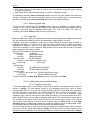
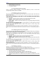
Nomenclature template looks like:
99 - 99 - 99 - 99
12 34 56 78
Character number
1
2
3,4
5,6
Meaning
Block or subsystem (1-9)
Scale (1-5)
Number of Latitude zone, Longitude zone of subsystem (00 - 24)
Number of Latitude zone, Longitude zone of 1:10 000 000,
1:5 000 000, 1:2 500 000, 1:1 000 000 maps (00 - 99)
7,8
Number of Latitude zone, Longitude zone of 1:1 000 000, 1:500 000,
(00 - 11)
Nomenclature samples:
© 2009
12
VectOr
Subsystem Europe:
Scale 1: 10 000 000: 11-01
Scale 1: 5 000 000: 12-01-10
Scale 1: 2 500 000: 13-01-21
Scale 1: 1 000 000: 14-01-53
Scale 1: 500 000:
15-01-53-10
1.4.1.2.3. Nomenclature of aerial navigation maps
Nomenclature template looks like
9 - 9 - 99 - 99
1 2 34 56
Character number
Meaning
1
Block (1 - main block, 2 - north pole block, 3 - south pole block)
2
Scale (1 - 1:2 000 000, 2 - 4 000 000)
3,4
“Longitude zone” (01 - 12)
5,6
“Latitude zone” (01 - 20)
Sample of nomenclature
The main block of a scale 1: 2 000 000: 1-2-10-05.
1.4.1.3.Work region
Usually, nomenclature sheets divide the source cartographic data used for maps of different
types and scales. Each sheet corresponds to exact area of the ground. It is necessary to
merge somehow several paper sheets to work with them as a whole.
The merging procedure is very simple in VectOr software. You can correctly display as many
as needed digital map sheets on the screen all together if they have the same scale and map
projection. At the same time each of them is still stored in separate file.
The collection of map sheets to be processed all together is called Work region.
13
RACURS Co., Ul. Yaroslavskaya, 13-A, office 15, 129366, Moscow, Russia
PHOTOMOD
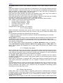
Digital maps database structure
All map sheets (nomenclature sheets), included to Work region, must have the same scale,
projection and coordinate system.
The data related to Nomenclature sheets is located in the following files:
• Metrics (coordinates of objects, *.DAT),
• Semantics (attributes of objects, *.SEM),
• Reference data (indices for fast searching object or its description, *.HDR).
There is one passport file (*.MAP) for the entire Work region that consists of records related
to each map sheet. All information related to object attributes and characteristics is stored in
digital classifier of work region (*.RCS file).
Work region is created when loading data form SXF file using DIR file (see Appendix A).
Any map sheet, included to work region can be edited, updated and passed from one user to
another separately of other work region map sheets. Data files, corresponding to one Work
region should be stored in one directory.
1.4.1.4.Structure of vector user maps
The structure of vector maps allows storing digital representation of real objects of region, as
well as user-related datasets that can be rapidly varied in time. The samples of such kind of
data are information about transportation network, weather forecast, etc.
To store these datasets you just have to add them to additional layers, object types, including
attributes in the map classifier. However there are some disadvantages in this way:
• user defined objects located on different map sheets are separated when saving and its
further processing is not convenient in most cases
• there is no way to view data, put on one map, on the other one for the same region
• it is necessary to expand and keep up-to date several map classifiers for the maps of
different types and scales
© 2009
14
VectOr
So VectOr allows to store “user” datasets separately of the “main” maps in special “user
maps”.
User map consists of just one map sheet of unlimited size. The size gets changed as some
objects are added / removed to/from map. The User map can be displayed along with Vector
map and Raster or Matrix maps. The same instance of User map can be visualized on
different Vector maps and edited by different users.
User map has its own classifier not equal to the classifier of the “main” map. The number of
displaying user maps along with the main Vector map is unlimited.
User map objects can not be linked to the user classifier. Objects of User map can be easily
imported from popular GIS systems via DXF or MIF/MID formats.
User map is rescaling appropriately when “moving” from one vector map to another.
Data, related to user map is stored in following files:
•
metrics (object coordinates, *.SDA),
•
semantics (object attributes, *.SSE),
•
information (index records, *.SHD),
•
map symbols (*.SGR).
Passport file for user map has *.SIT extension.
1.4.1.5. Group objects
Digital information associated with ground area is stored in separate map sheets. Real
ground objects and map symbols (map grid, contours, etc) can be located on different map
sheets.
For convenient work with such objects there are two ways:
• Using user maps, which contain one sheet of variable size depending on its contents
• Using group objects
Group object is a map object (real or conditional) which divided into map sheets but gets
combined every time it is opening (common object metrics is composed by single ones)
Once Group object is edited, it is automatically cut by map sheet borders. Map frames may
have arbitrary configuration.
You can create group objects automatically (in Sheets adjustment mode) or manually using Add objects to group, Remove objects from group options of Map editor icon
panel. Group objects are supported just in case when VECTOR.INI file contains string
Group=ON.
1.4.1.6.Graphic map object
Most of digital map objects are described in map classifier. Object description includes object
code, layer number, map symbol and other parameters. However when you need to put on a
map additional information (some comments, auxiliary lines, polygons) it is more convenient
to use simple graphic objects that are not attached to classifier.
So Graphic map object is an object that is not linked to classifier but has metrics,
semantics, unique ID and map symbol. Map symbol (pattern for lines and polygons) is stored
in object description.
When data is transferring in exchange SXF format map symbol is transferring along with
other object parameters (coordinates, ID, etc). Instead of external code there is a layer
number.
To put Graphic object on a map you should open appropriate user map or create a new one.
After this modes of map editor becomes available (creation of line, polygon, point, etc). Map
symbol parameters (line pattern, color, thickness, etc) are available in the dialog opened
according to current map editor mode.
1.4.2. Raster map structure
Digital raster map is a raster image of exploring ground area in defined scale, projection,
coordinate system. In fact raster image is 2D array of brightness values that can be acquired
in some spectral interval. Brightness can be represented by different number of “colors”
depending on raster type.
VectOr stores raster images in open RST format and supports import of raster objects from
15
RACURS Co., Ul. Yaroslavskaya, 13-A, office 15, 129366, Moscow, Russia
PHOTOMOD
PCX, TIFF, BMP and other popular formats.
The structure of raster VectOr file is as follows:
• passport data related to image (image size, raster type, color definition, etc)
• color map description
• raster image (raster map)
Working with raster images along with vector maps, you can easily update and edit any
digital information corresponding to exploring ground area.
RST file structure described in \DOC\SXF3-30.TXT.
1.4.3. Matrix map structure
VectOr handles matrix datasets (basically DEMs or feature maps) for the exploring region in
the open MTR format. MTR files contain additional data for the main VectOr SXF format to
represent different characteristics of the map region.
Matrix format has following structure
• passport data for the region
• feature matrix of region
There are two main types of the feature matrix:
• elevation matrix (DEM)
• feature matrix (thematic map)
Matrix can be built based on VectOr digital map vector objects. DEMs may contain absolute
heights of surface points, relative elevations or its summarized values (called attributes).
The feature matrix is created by searching vector objects based on user defined parameters.
The values of feature matrix are weight coefficients calculated by appropriate vector objects
parameters.
MTR file structure is described in \DOC\SXF3-30.TXT file.
1.5.
Scale range
One of advantages of digital maps versus paper ones is their displaying flexibility. You can
display and print digital maps in different scales, using different map legends and so on.
However, when using zoomed in map legend symbols or if the image is compressed when
scaling, some objects can cover other ones, causing problems in visual map perception.
There is a technology called Map generalization to make your digital map nice-looking and
more informative. One of the main generalization rules is to set visibility of every object
according to the current scale of displaying map. Scale range can be set for class of objects
(forest, lake, sidewalk, etc) when digital classifier is creating, it also can be redefined for any
single object by digital map editor tools. Besides user-defined scale range VectOr provides
automatic generalization procedure for different object categories. Starting at some scale
relative to the basic one, VectOr changes size of labels, removes relatively small objects,
changes thickness of polygon boundaries etc.
1.6.
VectOr installation
To start working you should install PHOTOMOD system or VectOr itself (in case of separate
VectOr purchasing). See also manual for PHOTOMOD system.
2.
VectOr interface
2.1.
Basic info
2.1.1. Start and exit
VectOr can be started from PHOTOMOD Montage Desktop module as well as separately
(VECTOR.EXE).
© 2009
16
VectOr
System is handling by mouse and keyboard. Screen is divided into work area, panels, menus
and messages area.
Once you have finished VectOr session, all maps get closed. All displaying parameters
including relative windows placement are saved in service INI files.
To exit VectOr, make one of following operations
• Double click on exit button of control menu;
• Select File/Exit option;
• Push F10 on keyboard.
2.1.2. Moving map image
To move an image in view window you can press “Pan” icon at the top menu and “grab” and
move window contents. In all other modes (editing, measurements...) you can just press left
mouse button and move cursor outside window to get image scrolling in corresponding
opposite direction. Another way is to press Shift key and move mouse cursor as needed. You
can also scroll a map, using keyboard: Ctrl and PgUp, PgDn, Home, End keys.
2.1.3. Moving cursor
You can move cursor using mouse or arrow keys along with Shift and Ctrl keys when cursor
is located over the map image.
2.1.4. Getting object description
To select object, click left mouse button or press Enter when mouse cursor is placed over the
object .The dialog Object selection is opened. Press Select button to select object (it will be
highlighted by red color). In case when there are several objects “under” mouse cursor you
can switch between them by Prev and Next buttons. The opened dialog allows viewing and
editing semantics, metrics, scale range and displaying style of the object. You can get
detailed information about the object by pressing Info button.
Once object is selected it can be edited, used in measurements, deleted, etc.
In case if some main panel dialogs is active when you select object, Object select dialog is
not opening and selected object starts blinking. You can see brief information related to
selected object in the top of map window. You can open Select object dialog by pressing
Spacebar when object is blinking.
To cancel object selection, press Esc key.
For fast object selection use Ctrl+left mouse button. In this case object will be selected
without opening the dialog.
The object metrics-related information includes:
• number of subobjects
• ID of displaying subobject
• number of points in object (subobject)
• distance between current and following point of object (subobject)
• azimuth angle between current and following point of object (subobject)
Metrics can be set using different units:
• meters in rectangular coordinate systems
• map units in rectangular coordinate system
• pixels in rectangular coordinate system
• radians in geodetic (geographic) coordinate system
• degrees in values range 1E-6 - 1E-7 in geodetic (geographic) coordinate system
• degrees, minutes, seconds in geodetic (geographic) coordinate system
If you edit object by changing distance and angle, coordinates of vertex that follows current
one are changed. You can not correct coordinates of the first object vertex this way.
To edit elevation values in object metrics first you have to open Full information window by
mouse double click over the dialog title or select Full info from pop-up menu that appears by
right mouse click over the dialog.
17
RACURS Co., Ul. Yaroslavskaya, 13-A, office 15, 129366, Moscow, Russia
PHOTOMOD
Using popup menu options you can also:
• revert object vertices numbering (including subobjects)
• revert vertices numbering for current subobject
• select current subobject
• set metrics accuracy.
2.1.5. Hot keys
You can use following hot keys while working with VectOr:
• View scale:
> - Zoom in;
< - Zoom out;
= - Initial scale.
• Moving view window over the map:
PgUp
- Move up at window size;
PgDn
- Move down at window size;
Home, Shift +Tab - Move left at window size;
End, Tab
- Move right at window size;
Ctrl+PgUp
- Move to the upper map border;
Ctrl+PgDn
- Move to the lower map border;
Ctrl+Home
- Move to the left map border;
Ctrl+End
- Move to the right map border;
Ctrl + up arrow
- Move up at 16 pixels;
Ctrl + down arrow - Move down at 16 pixels;
Ctrl + left arrow - Move left at 16 pixels;
Ctrl + right arrow - Move right at 16 pixels;
Shift + mouse moving - Move view window corresponding to mouse cursor position.
• Cursor moving:
Arrows
- Moving by 1 screen pixel;
Shift + Arrow - Moving by 8 screen pixels.
• Map operation. To start operations of editing, searching, measuring, etc., you should
click on corresponding icon.
Once operation is selected following hot keys become available:
Ctrl+C - To cancel current operation;
Ctrl + left button of the mouse - To complete operation.
• Map object selection:
Enter - To select nearest object to cursor (opens Object selection dialog).
If some operation is active when object selection selected object is blinking. Press
Enter again to go to the next object. Press Shift+Enter to go to previous object. Press
Ctrl+Enter to complete operation.
Space - opens Object selection dialog when object is blinking;
Ctrl+Enter - fast selection of closest to cursor object (without blinking and opening
dialog).
• Searching map objects:
Ctrl+F - Opens object Searching/Marking dialog;
Ctrl+L - Continues object searching starting at the last found one.
2.2.
“File” menu options
Menu File used to access to digital data in different formats.
© 2009
18
VectOr
Table 2.1 File menu options
Option
Meaning
New
Create map, user map, plan, matrix, etc.
Open
Open existing vector map, raster image or matrix
Map tree
Select a map from list
Add
Add to active map raster, matrix or user map
Close
Close map, raster or matrix
Update
Add and update data in active map
Save as...
Save map in selected format (BMP, DIR, MTW, SXF, TXT, ЕMF)
Print
Print a map or its fragment
Printer Setup
Select printer parameters
Exit
Exit VectOr
2.2.1. Creating digital map
2.2.1.1.Creating new map
To create a new map, select New/Map option of File menu. Dialog window consists of two
main parts (see below) appears:
• Area data
• Map sheet data
First fill area-related fields and press Add button. Obligatory parameters of map creation are
the name of resource (classifier) file (.RSC) and scale value greater than 0. Once Add button
is pressed Nomenclature dialog opens up. After entering Nomenclature (possibly using
special template) all map sheet related text fields become available.
Obligatory data for map sheet is coordinates (rectangular or geodetic). For topographic maps
of standard Nomenclature this fields get filled automatically. Otherwise coordinates must be
entered manually. For geographic maps there also should be filled fields of region passport
(standard parallels values, central meridian and origin latitude). Once all necessary fields are
filled out, you can close dialog or continue entering data for other map sheets.
You can also use Copy button for map creating. In this case you select existing map and
copy it to the created one for further editing.
Note that digital map passport can be edited any time using menu Tools/View Passport.
2.2.1.2.Creating plan
Plan in VectOr terminology is simple version of a digital map. Map in VectOr is a set of
digital information associated with some ground site and built by standard rules including
information about projection, nomenclature, vertical datum etc. Samples of map are
topographic, geographic or aerial navigation maps. Map passport must include all this
information. So in many cases it is easier and faster to create Plan (for example it is tourist
map of Lancaster county, NE). As a result you have digital map in which most of passport
fields are filled automatically.
To create plan, select New/Plan option of File menu. It is important to define what coordinate
system you are going to use for your plan. If it is large-scale cadastral scheme you can take
coordinates from source paper material. If you want have no information about source
coordinate system you should create your own one (local coordinate system). In this case
before scanning your paper map you should:
19
RACURS Co., Ul. Yaroslavskaya, 13-A, office 15, 129366, Moscow, Russia
PHOTOMOD
• add a rectangular border to map
• assign 0.0 coordinates to the low-left (south west) map corner
• calculate map scale (approximately)
Measure map size by X and Y axes and convert this distances to meters using scale factor. If
for example scale factor is 500 and rectangular X size = 25 cm and Y size = 50 cm you can
set following coordinates for plan corners
X southwest = 0.0,
X northwest = 125.0
X northeast = 125.0
X southeast = 0.0
Y southwest = 0.0,
Y northwest = 0.0,
Y northeast = 250.0,
Y southeast = 250.0.
Besides coordinate values you should set scale factor (500) and select classifier to be used
for plan. If creating Work region includes several map sheets you should at first create all
sheets separately and then combine them to Work region.
2.2.1.3.Creating user map
To create User map use File/New/User map menu.
You will need to enter its title, type and the name of used classifier (RSC file). Scale entering
is optional. Once User map passport is created, user map is adding to the “main” map,
which it will be used along with. First object can be added to User map just after it is
included to real map. At this step it is georeferenced to real map coordinate system and can
be opened as separate document (if needed) and get object added.
2.2.1.4.Creating matrix
There are several ways to open Matrix creation dialog:
• File/New/Matrix menu
icon in Map computer panel
•
• add non existing file to the matrix list
All information, related to current map and user map objects, is using when matrix creation.
Elevation matrix can be computed in fast mode
Elevation matrix can be computed for selected region or for selected map sheets.
To build matrix for the entire region set on All region option. To select some region portion
press Select button in Output area panel and select area you need by two clicks of left
mouse button.
Area borders can be also set by coordinate values in North, South, West, East text fields
Use Relief type menu to set a type of elevation calculations:
• absolute - matrix is calculated based on vector objects with True altitude attribute as well
as vector objects having Z coordinate in metrics
• summary - when output elevation values are calculating as a sum of absolute elevation
and elevation of vector objects with relative elevation attribute
In some cases there are several vector elements “under” creating matrix element. To define
how to calculate output elevation value Height if superposition menu is used. There are
two options in this menu:
• Maximum - maximum of “underlying” Z - coordinates is put to elevation matrix
• Average - average of “underlying” Z values is put to elevation matrix
There can be used auxiliary text file (MTRCREA.TXT) when matrix creation that contains
information related to vector objects used for computing elevation values.
You can set output matrix cell size (resolution) in Element size text field.
2.2.1.4.1.Fast mode of matrix creation
Elevation matrix can be computed in Fast or Normal modes. All matrix cells can be
separated to two groups:
© 2009
20
VectOr
• cells, which values are calculated at the first step of processing using information related
to vector map objects
• cells which values are calculated based on values of neighboring cells
The difference between Fast and Normal modes is that in first case smaller area and less
number of directions are used to calculate values of second group cells. So second group
cell values calculated by Fast and Normal methods may be slightly different.
2.2.2. Opening digital map
To open existing digital map, use File/Open menu. Now it is available for viewing, editing,
printing out, etc. You can open several maps at the same time and switch between them as
needed. If you open map in exchange format (SXF, TXT, DIR, PCX, BMP, TIFF, etc) it is
converting to internal VectOr format for further processing.
2.2.3. Map tree
Map tree (File menu option) is a hierarchical multilevel genealogy chart looking structure that
can be created and edited by user for fast searching needed map by its name.
Originally (right after installation), map tree is setup based on sample data included to
installation package. It is up to user to edit map tree or create new one. Map tree related
information is stored in .TRE file. The Map tree information for every map includes map
name and its location on your computer. Map location can be stored as full path or as partial
path associated with “parent” branch.
Below are the samples of valid map trees:
- General map
[E:\MAP\]
- Europe
[MAP1\EVR.MAP]
- America
[MAP2\US.MAP]
- Special maps
[D:\DATA\MAP\]
- A map of a site of the river [map1.map]
- A soil map
[terr.map]
And
- General map
- Europe
[E:\MAP\MAP1\EVR.MAP]
- America
[E:\MAP\MAP2\US.MAP]
- Special maps
- A map of a site of the river [D:\DATA\MAP\map1.map]
- A soil map
[D:\DATA\MAP\terr.map]
To edit a map tree use Add, Edit, Delete options of map tree menu Edit.
2.2.4. Loading data from external formats
2.2.4.1.Loading vector data
To create a digital map it is necessary to convert data, stored in exchange format, to internal
format of VectOr. To load dataset stored in the exchange format you have to select
corresponding SXF file. As a result of conversion MAP, HDR, DAT and SEM files, associated
with the map sheet, are created. You will also need RSC file to use it as a classifier. If you
use text version of SXF file it has TXT extension. If you use “file of directions” (DIR
extension) as a source it should load vector data according to its internal reference to RCS,
MAP and SXF files to include them to creating Work region. The name of Work region will be
set according to the name of the first SXF file or the name taken from DIR file. If you need to
select some vector objects to include to the creating map use Filter button to open Map
structure dialog. If loading map sheets are locating in adjacent zones of topographic maps
all coordinates will be recalculated to the first sheet coordinate system.
If some records can not be read from file they are skipped. Information about “bad” records is
put to the LOG file. When data loading, VectOr is verifying codes of source objects in the
classifier and the validation of its semantics attributes. In case of source data errors, VectOr
21
RACURS Co., Ul. Yaroslavskaya, 13-A, office 15, 129366, Moscow, Russia
PHOTOMOD
generates error message in LOG protocol. Objects having invalid classification code are
displaying by red outline. All attribute records associated with this objects will be started at
“*”-character.
2.2.4.2.Loading raster data
Raster objects needed to be included to the raster map can be loaded from one of the
following formats to VectOr raster format called RSW:
• BMP;
• PCX;
• TIFF.
To load raster image you should select appropriate raster file. Output RSW file will assign the
same name and .rsw extension.
Set the Scale and Resolution (dots per inch) parameters for output RSW file. Note that
these values can be changed during further processing.
To change all related to raster image parameters (Scale, Resolution, Color Map,
Georeference) use options of Raster list dialog.
2.2.4.2.1.Loading BMP files
Source BMP file must be standard Windows uncompressed BMP file. No restrictions for
image size and color map.
2.2.4.2.2.Loading PCX files
The source file should be standard PCX file. No restrictions for image size and color map.
2.2.4.2.3.Loading TIFF files
The source file should be standard TIFF file (version 6.0). No restrictions for image size and
color map.
2.2.5. Saving data
2.2.5.1.Saving digital map
Saving digital map causes saving all types of data (vector, raster, matrix) to appropriate files.
Saving procedure is also starting automatically according to time interval set in Parameters
menu (Redraw after).
Editing objects get saved directly to files after finishing each editing operation. All
intermediate situations are saved in auxiliary files in LOG directory. These files are cleaned
up after sorting map procedure.
2.2.5.2.Saving data in exchange format
Digital map can be saved in following exchange formats: SXF, TXT, BMP, EMF.
It is needed to convert vector data to exchange SXF format if you want to make the data
available for other applications or when you want to edit classifier (change object list, change
relations between objects and corresponding attributes).
It is possible to convert whole dataset to exchange format as well as copy just selected
layers, objects, object types, etc.
To filter (select) objects for conversion use Filter button which opens Structure of a map
dialog. Conversion procedure automatically creates DIR file, containing names of resource
file (RSC) and names of SXF files (in case of several map sheets) If program fails, all invalid
records are missing and program tries to process rest of them. Errors related information is
stored in LOG file.
To save vector map as a text file you should convert source data from internal VectOr format
to text version of SXF file. To do this you should select output file name and nomenclature of
saving map (if there are several map sheets included). Default output filename is equal to
© 2009
22
VectOr
input map file name.
You can save any fragment of digital map in BMP and EMF formats for further processing in
external applications. Matrix and raster data are saved in EMF format as rasters. Vector data
can also be saved either as raster (normal mode) or as vector (printer mode). See View
menu options.
2.2.6. Map upgrading
Map upgrading procedure adds to current map new objects, retrieved from SXF file. The
Map, taken from SXF file, should have the same scale, projection and nomenclature as the
upgrading one. If object, derived from SXF file, has unique id, equal to id of some object on a
map, this object will be replaced. All other objects just get added to the map.
SXF file can be either text (TXT) or binary (SXF) If current map does not contain a map sheet
corresponded to SXF file, this sheet will be loaded to the map and the Work region is
expanded. You can update raster dataset by loading new raster objects from BMP, PCX or
TIFF format to current digital map.
2.2.7. Printing a map
To print a map (or its selected fragment) you need:
• turn on the printer;
• press Print button.
Once printing is over you get an appropriate message (press OK).
It may take from several seconds to tens of minutes to print a map, depending on map size,
computer resources, printer type and printing quality.
Only objects selected by View contents dialog are sent to printer. There are several modes
of printing used to print a map:
• Normal - creates hardcopy of variable filling intensity of polygons used to print on color
and grayscale raster printers.
• Transparent - creates hardcopy without filling polygons, used to print to any (including
vector) output printing devices
• Outline - printing vector elements by lines on any printers;
There is a possibility to print the whole map as well as its portion. To select print area press
Select button and select map region by mouse.
VectOr supports changing the scale when printing. In Fit to page mode the output scale is
calculated automatically to fit current paper size. Map is divided into pages according to page
size, page orientation (Portrait or Landscape) and page margins. You can view output page
layouts in Print dialog
To select printer and set its parameters use Printer setup option.
To print map border (by black color) set Print border option on.
There are three radio buttons below the view area located in the upper-left part of Print
dialog:
• Map - shows map in details in view area
• Scheme - shows map border in view area to see its relative position when printing (fast
visualization)
• Information - shows map related info in view area
Possible problems with printing often caused by:
• not enough space for print file that created on disk where MS Windows is installed
• using wrong printer driver (for example PostScript).
2.3.
“Edit” menu options
Edit menu used to pass datasets to other applications via clipboard and graphic files.
23
RACURS Co., Ul. Yaroslavskaya, 13-A, office 15, 129366, Moscow, Russia
PHOTOMOD
Table 2.2. Edit menu options
Option
Meaning
Undo
Cancels last executed operation
Copy
Copies selected fragment to clipboard
Copy to
Copy Map window
Copies selected fragment to EMF or BMP file
Copies contents of current active window to clipboard
Copy Map window to
Copies contents of current active window to EMF or BMP file
2.4.
“View” menu options
View menu used to set options for currently open map viewing.
Table 2.3. View menu options
Option
Meaning
View Contents
To select objects to be displayed
Map image
Type of visualization (normal, draft, printer, printer outline)
Matrix image
Type of matrix visualization (color or grayscale)
Raster list
Changing raster displaying parameters
Matrix list
Changing matrices displaying parameters
User Map
Changing user maps displaying parameters
Embedded Object
2.4.1. View contents (Map structure)
The dialog box Map structure used to select objects for displaying by different criteria. Map
object are structured as follows:
• Map layers and object types
• Object styles
• List of map sheets
• Range of object IDs
• Objects attributes (semantics)
• Spatial object parameters
Full list of map layers, object types, object attributes are defined by Map classifier.
To select layers to be displayed you should open Map structure/Layers dialog and select
needed layers in the list by mouse.
To select map sheets to be displayed open Map structure/Map sheets dialog and
select/unselect map sheets in the list by mouse.
To set range of displaying object IDs open Map structure/IDs dialog and set minimum and
maximum ID of displaying objects.
To set criterion for object displaying based on its attributes open Map structure/Semantics
dialog and set on Selected semantics option. If, for example, you want to display objects,
that have absolute elevation > 100m you need to build an expression like this Absolute
elevation > 100. To do it use dialog panel consists of three columns: Semantics code
name, Condition, Value. Press Selected semantics to select attribute name (Absolute
altitude). Double click on Condition to select > and type 100 in Value text field.
To set selection by spatial object parameters open Map structure/Measurements dialog.
Press Selected measurements button. Set type of measurement (for example length). Set
condition like length < 100 in Single mode or 50 < length < 250 in Range mode. To set
condition use Expression panel.
You can use Model dialog to create several models of object selection (set by dialogs listed
above). To create model, press Create button to add model to Model list (up to 256
models). Selection models are saved once VectOr session is over and restored when
system starts another time.
© 2009
24
VectOr
2.4.2. Map displaying mode (Map image)
The vector map can be displayed in several ways:
•
Normal - all digital map objects are displaying in accelerated mode according to the
map legend stored in the digital classifier.
•
Draft - objects are displaying in draft simplified form
•
Printer - map looks completely like its hardcopy using full library of output styles
•
Printer outline – polygons look like not filled.
2.4.3. Raster displaying parameters (Raster list)
Used to add, remove, change properties of raster objects included to map:
• raster view modes (full, saturated, translucent, average, transparent, none)
• raster color map
• raster relative position on digital map. You can place raster relatively to current vector
map using following methods:
- place raster by one point,
- place raster by two points with scaling,
- place raster by two points with scaling and rotation,
- move raster to southwest map corner
These modes are available in Raster list/Properties menu
• current raster position in view window;
• scale
• resolution
• optimization (optimization speeds up raster displaying and reduce required disk space
for) raster storing.
• color view preferences
When adding rasters of BMP, PCX, TIFF formats, corresponding converter to internal RSW
format is started. Multi-selection mode is also available.
2.4.4. Matrix displaying parameters (Matrix list)
Matrix map can be displayed using two modes:
• Color map
• Grayscale
In case of color map color range from deep-green (low elevations) to deep-brown (high
elevation) is used. In case of grayscale low elevation pixels look dark and high elevation
pixels look bright.
2.4.5. User map displaying parameters
User map list menu used to change a structure of the list of files of user maps, and
properties of a user map selected in the list of files. To access user map parameters use
right mouse button or Properties button. User has possibility to not display a user map and
change a structure of displayed layers and objects.
2.5.
“Search” menu options
Search menu used to select map objects based on different parameters.
Table 2.4. Search menu options
Option
Meaning
Search and mark
Searching and marking map objects, using query based on
classifier
25
RACURS Co., Ul. Yaroslavskaya, 13-A, office 15, 129366, Moscow, Russia
PHOTOMOD
Option
Search by query
Meaning
Searching object by query
Search by area
Searching by selected area
Search again
Searching object based on conditions selected for previous
searching session
2.5.1. Search and mark objects
Dialog Search object allows to use set of parameters for object searching:
• map layers and object classes
• object types
• map sheets (Nomenclatures)
• range of object IDs
• object attributes (semantics)
• spatial object parameters
Full list of map layers, object classes, object types, object attributes, is defined by Map
classifier.
To select layers to be marked you should open Map structure/Layers dialog and selects
needed layers in the list by mouse.
To select map sheets to be marked open Map structure/Map sheets dialog and
select/unselect map sheets in the list by mouse.
To set range of marking object IDs open Map structure/IDs dialog and set minimum and
maximum ID of marking objects. To set criterion for objects selection, based on their
attributes, open Map structure/Semantics dialog and set on Selected semantics option. If
for example you want to display objects that have absolute elevation > 100m you need to
build an expression like this Absolute elevation > 100. To do it, use dialog panel consists of
three columns: Semantics code name, Condition, Value. Press Selected semantics to
select attribute name (Absolute altitude). Double click on Condition to select > and type 100
in Value text field. To set selection by spatial object parameters open Map
structure/Measurements dialog. Press Selected measurements button. Set type of
measurement (for example length). Set condition like length < 100 in Single mode or 50 <
length < 250 in Range mode. To set condition use Expression panel. You can use Model
dialog to create several models of object selection (set by dialogs listed above). To create
model, press Create button to add model to Model list (up to 256 models). Selection models
are saved once VectOr session is over and restored when system starts another time.
2.5.2. Searching objects by query
When searching objects by query you should use following searching parameters:
• map layers and object classes
• object types
• map sheets (Nomenclatures)
• range of object IDs
• object attributes (semantics)
• spatial object parameters
Full list of map layers, object classes, object types, object attributes, is defined by Map
classifier.
To select layers to be marked you should open Map structure/Layers dialog and selects
needed layers in the list by mouse.
To select map sheets to be marked open Map structure/Map sheets dialog and
© 2009
26
VectOr
select/unselect map sheets in the list by mouse.
To set range of marking object IDs open Map structure/IDs dialog and set minimum and
maximum ID of marking objects. To set criterion for objects selection, based on their
attributes, open Map structure/Semantics dialog and set on Selected semantics option. If
for example you want to display objects that have absolute elevation > 100m you need to
build an expression like this Absolute elevation > 100. To do it, use dialog panel consists of
three columns: Semantics code name, Condition, Value. Press Selected semantics to
select attribute name (Absolute altitude). Double click on Condition to select > and type 100
in Value text field. To set selection by spatial object parameters open Map
structure/Measurements dialog. Press Selected measurements button. Set type of
measurement (for example length). Set condition like length < 100 in Single mode or 50 <
length < 250 in Range mode. To set condition use Expression panel. You can use Model
dialog to create several models of object selection (set by dialogs listed above). To create
model, press Create button to add model to Model list (up to 256 models). Selection models
are saved once VectOr session is over and restored when system starts another time.
2.5.3. Searching objects by selected area
To search map objects by selected area you should select area and set searching
parameters. Use mouse to select area on a map and complete operation (see 3.2.1.7
section).
Then you have to select searching parameters:
• search inside/outside area
• searching distance (used in «outside» mode)
• filter (object selection by layer, type, attributes, etc)
2.5.4. Searching objects by name
This mode is used to search objects by value of selected attribute. To set attribute
(semantics) name used by searching operation press Setup.. button and select semantics by
double click or OK button. You can also manually enter semantics name (By name mode) or
semantics code (By number mode) in Search semantics text field. You can type just first
characters of attribute name (code) for speeding up (for example “Lancast” instead of
“Lancaster” or «167» instead of «167523»). All dialog parameters (attribute values) are
saved and restored for next Searching sessions.
2.6.
“Tools” menu options
Table 2.5. Tools menu options
Option
Meaning
Map Editor
Editing vector map
Map Computer
Measurements over digital map
Map Navigator
Navigation through digital map
Map Sorting
Sorting (and compression) data
View Passport
Viewing and editing map passport
Map classifier
Editing and adding object attributes and map symbols
Run Application
Running application tasks
27
RACURS Co., Ul. Yaroslavskaya, 13-A, office 15, 129366, Moscow, Russia
PHOTOMOD
You can find a description of such programs as map editor, measurements on the map, map
passport in Basic application tasks section.
Run application dialog consists of three main parts:
• task name
• path to corresponding DLL file
• control icons
Use Add and Delete buttons to add and remove tasks from list. To run application, press
Start button. If some task is currently executing there is a checker near its name in the list.
Some DLLs also additionally marked by icon.
2.7.
“Scale” menu options
Used to scale a map on the screen.
Table 2.6. “Scale” menu options
Option
Meaning
Zoom In
Zooming in map by left mouse button
Zoom Out
Zooming out map by left mouse button
Full
Zoom 1:1
Display full map
Display map in 1:1 scale
There also two ways to change map scale:
•
press < or > keys to zoom in, zoom out map respectively;
•
select zooming mode by right mouse button.
2.8.
“Options” menu options
Table 2.7. “Options” menu options
Option
Meaning
Coordinate System
Selecting coordinate system
Colors
Selecting palette for map displaying
Fonts
Selecting fonts used in map displaying and dialogs
Screen Options
Screen size and image scale
Language
Language, used in interface (English or Russian)
Redraw after (s)
Period of digital map updating
There are following coordinate systems available:
1. Rectangular in Meters.
2. Rectangular in Map units.
3. Rectangular in Pixels.
4. Geodetic (Radians).
5. Geodetic (Degrees).
6. Geodetic (Degrees, minutes, seconds).
© 2009
28
VectOr
2.8.1. Map palette
Used to set colors and brightness/contrast parameters of a map including vector and raster
information.
Color palette dialog includes following panels:
• Service - used to set colors of map background, selected objects, marked objects and
thickness of line for vector object displaying.
• Map - used to set colors for map displaying as well as brightness/contrast parameters. To
change color in map palette click on the appropriate one in the color map and change it
as needed.
• Raster - used to set raster color map as well as raster brightness/contrast parameters.
To change color in color map click on appropriate one on the color map and change it as
needed.
• Matrix - used to set matrix color map as well as matrix brightness/contrast parameters.
To change color in color map click on appropriate one on the color map and change it as
needed.
2.8.2. Setting fonts
You can set fonts for map labels as well as fonts, used by dialogs.
Screen fonts dialog allows you to set fonts used by map displaying and raster output
devices. Plotter fonts dialog allows you to set fonts for printing to vector output devices
(plotters).
2.8.3. Image size and scale
Digital map can be displayed in different scale. There is a current scale value at the bottom
part of the main window. However visual object size, distance between objects on screen,
height of label letters may not correspond to the paper samples. It also can depend on
monitor type. It happens because MS Windows does not determine physical size of screen
pixel but printer devices do. You can use Screen options dialog to set Screen size (default
value (diagonal) is 1.5 inches less than passport one) and Zoom factor. Image increasing
makes a map more viewable but changes its real scale. If diagonal value is set correctly and
zoom factor is equal to 100%, the accuracy of image displaying is 0.5 pixel. Map symbols are
displaying it its real size when displaying scale is equal to the map scale. Displaying scale
changing causes appropriate changes in map symbol size.
MAP DISPLAYING PARAMETERS DO NOT CAUSE CHANGES IN CALCULATIONS OF
COORDINATES, DISTANCES, AREAS, etc.
2.9.
“Window” menu options
Window menu options used to handle user-interface elements on the screen.
Table 2.8. Window menu options
Option
Meaning
To display windows as a cascade
Cascade
Mosaic
29
To display windows as a mosaic
Arrange Icons
To put all icons to a row
Close All
To close all open documents
RACURS Co., Ul. Yaroslavskaya, 13-A, office 15, 129366, Moscow, Russia
PHOTOMOD
2.10. “Help” menu options
There are two choices under Help menu: Information (opens VectOr’s help) and About,
that opens panel containing following information:
•
Program name;
•
Program version;
•
Hardware key ID;
•
Mail address of software developing company;
•
Web-site;
•
E-mail address.
3.
Basic application tasks
3.1.
Editing passport of vector map
To edit passport of the map, select View Passport option from Tools menu.
Map passport consists of datasets related to Work region and Map sheet.
The Work region dataset includes:
1. Title of area;
2. Source data:
• Type of a map;
• Scale;
• Name of resource file;
3. Projection data:
• Ellipsoid;
• Vertical datum;
• Coordinate system;
• Source projection;
• 1st standard parallel;
• 2nd standard parallel;
• Central meridian;
• Origin latitude;
4. Area extents;
5. Additional information:
• Plane and elevation units
• Digitizing rate;
• Type of a framework;
Not editable records:
• Resource file name (since it is created only when passport creation)
• Scale;
• Area extents, since they are calculated automatically by map sheet extents
If map type gets changed you get a warning that data are in wrong projection. So it is not
recommended to edit Map type.
Map sheet data set includes:
1. Nomenclature (sheet title);
2. Coordinate of the sheet (rectangular and geodetic);
3. Data related to a map document:
• Sort and type of the initial map document;
• Date of survey;
4. Declination data:
• Magnetic declination;
• Average meridian convergence;
• Annual magnetic declination;
• Date of measurement of the declination;
5. Data files name (the name is common for all data files with HDR, DAT, SEM, GRA
© 2009
30
VectOr
extensions.
All map sheet related data sets can be edited except Nomenclature since it is constant for
standard map sheets. You also must not edit coordinates for this type of maps.
Once Add button is pressed new dialog window gets opened. You need to enter map sheet
nomenclature using standard template (if needed). When dialog Input of nomenclature is
closed input data fields appear on screen.
Coordinates data fields should be filled obligatorily. In case of standard map sheets (with
known nomenclature) this fields are filled out automatically. In all other cases you should
enter coordinate values manually. For geographic map, it is also necessary enter projection
related data, including 1st and 2nd standard parallels, central meridian, origin point latitude.
Once all necessary data is input you can either close the dialog or continue input adding new
map sheets.
3.2.
Vector map editor
To activate vector map editor select Tools|Map Editor option.
Vector map editor is an integrated part of VectOr system and used to creation and editing
digital vector maps.
There is a panel of icons located along the left screen border. Each icon corresponds to
option of vector map editor. You have to push the appropriate icon to activate editing mode
you need. In case when you are working in one editing mode and do not finish the editing
operation all other icons are not available.
Once editing is completed the vector object is saved to file automatically.
If program failures during the input and editing, data is not lost.
All displaying options (such as color, scale, background, view contents) are available when
editing and can be changed any time you need.
Map editor functions are as follows:
• Select object type
• Create point object
• Create line object
• Create polygon object
• Create label
• Create object with existing code
• Create object group by coordinates from file
• Save conditional object
• Create object layouts
• Delete selected object
• Delete one subobject
• Delete all subobjects
• Move object
• Full copy (backup) of object
• Edit vertex
• Create node
• Delete vertex
• Close object
• Edit label
• Change object type
• One step undo
• Create subobject
• Copy portion
• Delete marked object
• Restore deleted objects
• Edit common vertices of adjacent objects
• Rotate object
• Copy object to user map
31
RACURS Co., Ul. Yaroslavskaya, 13-A, office 15, 129366, Moscow, Russia
PHOTOMOD
•
•
•
•
•
•
•
•
•
•
•
•
•
•
•
•
•
•
•
•
•
•
•
•
•
•
Add vertex
Intersect objects
Merge objects
Copy all subobjects
Copy marked objects to user map
Joining vertices
Dissection of line object
Joining line objects
Delete panel
Group panel
Topology panel
Restore edited objects
Parameters of edit session
Code conversion of marked objects
Filtering objects
Smoothing objects
Point panel
Creation panel
Panel Processing semantics of marked of objects
Add semantics to marked objects
Delete semantics of marked objects
Replace semantics of marked objects
Text panel
Selection panel
Expand line object
Classification.
3.2.1. General information
3.2.1.1.General information related to object editing
All editing operation can be executed for selected object. See detailed description of object
selection in 3.8.1.3 section. Only one object can be selected at once. When editing (or
creating) is done object is still selected so you can switch to another editing tool. If you want
to begin editing another object just select it by standard way.
Some operations are implemented for object group (for example Deleting marked objects).
In this case you should previously mark (do not confuse Mark mode with Select mode)
objects using Search menu tools.
Although there is a Save as option in File menu, you should not save your map after editing.
Edited object gets saved right after its editing is completed. It’s possible to return to previous
statuses of map unless it is sorted.
3.2.1.2.Map editor options
Map editor options are as follows:
• Cut objects by map sheets: objects that cover several map sheets in work region will
be cut by every sheet border.
• Cut objects by parent frame: objects that cover several map sheets in work region
will be cut by the frame where the first object vertex located.
• Use semantics when object creating. Adding semantics when object creating.
• No frame editing. Frame editing causes changes of map georeference and may have
unexpected effect.
• Tracing rate parameter of smoothing vector line created by interactive vectorization
(tracing) over raster image
• Zone width - Width of creating object - parallel line. Zone width can also be changed
© 2009
32
VectOr
•
•
•
by «+» and «-» keys
Joining tolerance - tolerance of joining corresponding objects located on adjacent
map sheets. If the distance between corresponding vertices is greater then tolerance
value objects will not be combined.
Filtering level - distance between object vertex and line segment connecting previous
and next vertices. If this distance is less than Filtering level parameter this vertex is
removed by line filtering operation (decreasing number of line vertices).
Recommended value is 1.5.
Spline order used for line smoothing operation.
3.2.1.3.Object selection
To select object, click left mouse button or press Enter when mouse cursor is placed over the
object .The dialog Object selection is opened. Press Select button to select object (it will be
highlighted by red color). In case when there are several objects «under» mouse cursor you
can switch between them by Prev and Next buttons.
Once object is selected it can be edited, used in measurements, deleted, etc.
In case if some main panel dialogs is active when you select object, Object select dialog is
not opening and selected object starts blinking. You can see brief information related to
selected object in the top of map window. You can open Select object dialog by pressing
Spacebar when object is blinking.
To cancel object selection, press Esc key.
For fast object selection use Ctrl+left mouse button. In this case object will be selected
without opening the dialog.
3.2.1.4.Unselecting objects
To unselect an object you can
• Select new one
• Press Cancel button on Select object dialog
• Press Ctrl and right mouse button
• Press Cancel on pop-up menu opened by right mouse button.
3.2.1.5.Selecting object part
You can select a portion of object by selecting 2 (for non-closed line) or 3 (for closed line)
metrics points using left mouse button. This mode can be used for editing or making
measurements when message string is Select part of object.
3.2.1.6.Editing object part
Select object part by three points and edit object part point by point (move them to a new
position). To complete editing – press Ctrl key and left mouse button. To go back use Step
back or Restoring edited object.
3.2.1.7.Completing operation
To complete operation (for example calculate segment length or save line) you can:
• press Ctrl+Enter
• press Ctrl+left mouse button
• press right and left mouse buttons
• press Yes or OK in appropriate dialog
If you complete object creation by double click, additional vertex is created. Otherwise not.
3.2.1.8.Canceling operation
To cancel any operation you can:
33
RACURS Co., Ul. Yaroslavskaya, 13-A, office 15, 129366, Moscow, Russia
PHOTOMOD
•
•
•
•
•
click again on the same icon to get it released
select another operation
close corresponding task in Tools menu
press Ctrl+right mouse button (if currently some object is selected it is at first
deselecting and you have to press Ctrl+right mouse button again to cancel operation)
using pop-up menu opened by right mouse button.
3.2.1.9.One step Undo
Restores previously edited or deleted object.
3.2.2. Object creation
3.2.2.1.Object creation modes
Object creation menu includes following modes:
• Create object (object type is selected from map symbols library);
• Create object of type of existing object;
• Create subobject;
• Copy object;
• Copy object to another map (object type is selected from map symbols library);
• Copy marked objects to another map;
• Save object created by another application.
• Create graphic objects (line, polygon, raster symbol, label).
3.2.2.2.Creation of map object
To create map object you should define corresponding map symbol (object style), its spatial
coordinates (metrics) and attributes (semantics). Object style is created in special dialog that
also allows you to set method of object creation (manual or interactive vectorization, manual
coordinates entering, loading coordinates from text file, etc). The sample of object is
displaying in special view window. You can use fast object searching by its name or
classification code. If object type and layer are selected you can use Ctrl and Shift keys to
make group object selection. For example you can select all line and polygon objects from
layers called Road network and Road facilities. Press Select button for final object style
selection. Besides, you can select object style from Map legend panel. You can attach
attributes (add semantics) when object selection if corresponding option of Map editor is on.
3.2.2.3.Point object creation
Point object of a digital map contains coordinates of one point. The point object can be
spatially connected to other objects of a map (see Supplementary creation modes section)
To put point object on the map press left mouse button. Its location can be changed unless
left mouse button is released.
3.2.2.4.Line object creation
The line object of a digital map contains coordinates of two or more points.
Line object can be closed or non-closed, it can include several subobjects and spatially
connected to other objects of the map
Depending onto its type line object can be created as one of following:
•
object of arbitrary configuration
•
simple, rotated or complex rectangle
•
circle of known diameter
•
result of interactive vectorization (tracing) over underlying raster
•
entering coordinates from keyboard
•
loading from text file
Line object points (vertices) are creating when pressing left mouse button or Enter. To close
© 2009
34
VectOr
line object press L button. Supplementary modes of creation are also available
To save line object use standard save operation (see 3.2.1.7 section).
Pressing Backspace key deletes last added vertex.
To create a rectangle you should “draw” it on the map using left mouse button.
To create a rotated rectangle you should “draw” it on the map using left mouse button.
To create a complex rectangle you should add its vertices one by one by left mouse button
(all line segments are intersected at the right angle).
To save any line objects, use standard save operation (see 3.2.1.7 section).
To create a circle of fixed radius you need to set its radius and center point. You can use
previously created point object as a center for circle as well as any line vertex. (Refer to
Supplementary modes of creation section for details)
To create an arbitrary circle you need to draw it by left mouse button. You can use
previously created point object as a center for circle as well as any line vertex. (Refer to
Supplementary modes of creation section for details)
Vectorization (tracing) is a process of interactive following line features of raster image to
convert them to vector format. To start vectorization you need to set first line vertex by left
mouse button or copy it from existing object. To start automatic procedure you should set the
direction by mouse cursor and press O key. To save vector line use standard save operation
(see 3.2.1.7 section).
3.2.2.5.Polygon object creation
Polygon object of a digital map is a closed polyline. Displaying style of polygon is defined in
map classifier. Besides main (exterior) boundary, polygon can include «islands» subobjects. Polygon can be spatially connected to other map objects.
Depending onto its type polygon can be created as one of following:
• object of arbitrary configuration
• simple, rotated or complex rectangle
• circle of known diameter
• result of interactive vectorization over underlying raster
• entering coordinates from keyboard
• loading from text file
Polygon object points (vertices) are creating when pressing left mouse button or Enter.
Polygon object is closed automatically. Supplementary modes of creation are also available
To save line object use standard save operation (see 3.2.1.7 section).
Pressing Backspace key deletes last added vertex.
To create a rectangle you should «draw» it on the map using left mouse button.
To create a rotated rectangle you should «draw» it on the map using left mouse button.
To create a complex rectangle you should add its vertices one by one by left mouse button
(all polygon segments are intersected at the right angle)
To save any polygon objects, use standard save operation (see 3.2.1.7 section).
To create a circle of fixed radius you need to set its radius and center point. You can use
previously created point object as a center for circle as well as any polygon vertex. (Refer to
Supplementary modes of creation section for details)
To create an arbitrary circle you need to draw it by left mouse button. You can use
previously created point object as a center for circle as well as any polygon vertex. (Refer to
Supplementary modes of creation section for details)
Vectorization (tracing) is a process of interactive following line features of raster image to
convert them into vector format. To start vectorization you need to set first polygon vertex
by left mouse button or copy it from existing object. To start automatic procedure you should
set the direction by mouse cursor and press O key. To save vector line use standard save
operation (see 3.2.1.7 section).
3.2.2.6.Creating object with the code of existing object
To create object with the code of existing object you should select existing object first and
35
RACURS Co., Ul. Yaroslavskaya, 13-A, office 15, 129366, Moscow, Russia
PHOTOMOD
then create a new one.
3.2.2.7.Creating object group by coordinates, retrieved from file
You can create object (or group of objects of common type) which described in text file as a
set of coordinates of vector elements. First you have to prepare text file appropriately:
• text file has to have .MET extension
• text file must not to have empty strings
• text file may have service fields
Field
MET
BEGIN
#
END
XY
RAD
GRAD
GMS
/
Function
File beginning keyword
Information beginning keyword
Object beginning keyword
end information keyword
Rectangular coordinates (m.)
Radians
Degrees in decimal form
Degree, minute, second
Comment string
Note
a mandatory field
a mandatory field
a mandatory field
a mandatory field
Service fields must start at the first string position
- MET, BEGIN, END are mandatory keywords, the description of object description is
delimited by #.
- Strings located between «#» symbols must contain only coordinate values or comments
strings.
- By default (or if coordinate section marked as XY) coordinate values are in rectangular
coordinate system (after «#» symbol there are strings containing coordinate pairs
corresponding to object points (m))
- After RAD keyword there are pairs of vector point geodetic coordinates (B, L) in radians
- After GRAD keyword there are pairs of vector point geodetic coordinates (B, L) in decimal
degrees
- After GMS keyword there are pairs of vector point geodetic coordinates in Deg Min Sec
format.
Note that the range of possible latitude values is from -90(south) to 90(north) degrees and
the range of possible longitude values is 0 - 360 degrees.
Sample of a text file:
MET
BEGIN
// Point objects (radians)
RAD
#
0.97065938 0.65882652
#
0.97058971 0.65838004
// Point objects (Decimal degrees)
GRAD
#
55.65802244 37.54409293
// Point objects (meters)
XY
#
6171257.20 7408038.50
#
6169977.20 7407298.50
© 2009
36
VectOr
// Point objects (Degrees Minutes Seconds)
GMS
#
55 39 28.88 37 32 38.73
#
55 39 18.96 37 32 20.51
END
To add object to map use By coordinates from text file mode of Object creation dialog.
3.2.2.8.Creating subobject
To create subobject (island of polygon or part of line) select parent object and create
subobject line or polygon by standard way.
3.2.2.9.Creating vector object from conditional object
This mode is used to reassigning attributes to the object created by some VectOr
application. For example when buffer zone is built around selected vector object. To save
conditional object you have to select object type by the same way as when creating new
vector object.
3.2.2.10.Supplementary modes of object creation
The supplementary object creation modes are used to provide spatial topological
relationships between objects that can belong to one or different map layers. Using
supplementary object creation modes you can copy existing point or object portion to
creating object with or without node creation. To activate supplementary object creation
mode use corresponding option of pop-up menu or appropriate keyboard key.
Supplementary object creation modes include:
• I - copying real point. This mode is useful if you want to create object that exactly
goes through already existing ones. For example you «draw» electric power line
connecting existing piers (point objects). To activate Copying real point mode, press
I key. Then select object, used for snapping to, and start drawing. Press I for each
vertex should be snapped to existing point. You can use any objects to be snapped to
(in case of lines and polygons their vertices are used for snapping).
• T - copying pseudo-point with node creation. This mode is pretty much similar to
previous one, but now you use not existing vertex for snapping to, it can be located
anywhere on selected line. In other words this mode works like snapping to object and
previous one provides snapping to object vertices. Node is created in every snapped
vertex in this mode.
• D - copying pseudo-point without node creation. Mode is just like the previous
one, but without node creation. It can be useful when created object is snapping to the
map border and there should not be nodes on it.
• K - copying fragment of object bounded by pseudo-points. This mode is useful if
created and existing objects should have common part (fragment). Fragment selection
is making by 3 points - (start, middle, end of fragment). Second point can be equal to
the first or third one. So in this case only 2 points are used for fragment selection.
However if source object is a polygon always use 3 points. Once copying is done
nodes are created at the first and third snapping points.
• P - copying fragment of object bounded by real points. Mode is similar to previous
one, except that, only vertices can be used for fragment selection.
• H - creating horizontal line. Mode of horizontal line drawing (X=const).
• V - creating vertical line. Mode of vertical line drawing (Y=const).
• F - cancellation of modes H and V.
• R - current raster selection (for interactive vectorization(tracing)). While tracing, it is
possible to create an object over several opened rasters.
• M - memorizing cursor position on a map.
• N - go to the previous (saved by M) point.
37
RACURS Co., Ul. Yaroslavskaya, 13-A, office 15, 129366, Moscow, Russia
PHOTOMOD
•
O - starting interactive vectorization (tracing).
3.2.2.11.Map legend
You can create map legend including most usable map objects for fast and convenient
access to them. VectOr map legend located at the bottom of screen and looks like rows of
pictograms (up to 255 lines) with map symbols associated with map objects. Every row of
map symbols has unique name for convenience of object searching. Once legend is created
you don’t need to open complicated Classifier dialog to search and select map object. Just
click on corresponding pictogram in map legend row.
To show map legend click on corresponding icon of Map editor panel.
When map legend is opened first time, all pictograms have gray cross on them, which will be
replaced by appropriate map symbol when created. To add map symbol to legend press any
pictogram and select map symbol.
Note that map legend is linked to map classifier, so if classifier is edited you should recreate
map legend (you will get appropriate system warning).
3.2.3. Deleting objects
3.2.3.1.Deleting selected object
Once an object to be deleted is selected, you get warning message to confirm delete
operation. Press OK to delete object. You can restore it using Undo operation.
3.2.3.2.“Delete” panel
Delete panel includes following modes:
•
deleting one subobject;
•
deleting all subobjects;
•
deleting marked objects.
3.2.3.3.Deleting one subobject
This mode is used to delete an island (subobject of polygon). To execute operation you
should select polygon and its subobject.
3.2.3.4.Deleting all subobjects
This mode is used to delete all islands (subobjects of polygon). To execute operation you
should select parent polygon.
3.2.4. Map objects editing
3.2.4.1.Changing code of marked objects
Changing code of marked objects used to access new map symbol to the group of objects.
When reassigning map symbol all object parameters (name, attributes, etc) may be changed
except its coordinates.
3.2.4.2.Copying object to user map
To copy object to user map you should select object to be copied and select destination map
and output object type (since source and output maps can be linked to different classifiers).
3.2.4.3.Copying all subobjects
Used to copy all subobjects (islands) on one polygon to another polygon. To copy you should
select source and destination polygons and complete operation (see 3.2.1.7 section). To
cancel operation, use 1 step undo or Cancel button of Edit menu.
© 2009
38
VectOr
3.2.4.4.Full copy of object
To copy object, select it and set a new object position in drag-and-drop mode. Use arrow
keys along with left mouse button pressed for precise object positioning. Object is saving by
standard save operation (see 3.2.1.7 section).
3.2.4.5.Moving object
To move object, select it and set a new object position in drag and drop mode. Use arrow
keys along with left mouse button pressed for precise object positioning. Object is saving by
standard save operation (see 3.2.1.7 section).
3.2.4.6.Changing object type
To change object type you should select object and set its new type.
3.2.4.7.Expanding vector line
To expand (continue digitizing vector line) select it. As a result the cursor is located at the
last object vertex (defined by vertices numbering order). If you need to add vertices in the
opposite direction press R key. Then «draw» vector line in standard way. All additional object
creation modes are available.
3.2.4.8.Marking (grouping)
Used to mark objects on the map manually. Every marked object is added to object group for
further possible group processing (delete group, copy group, decode group, move group to
another map and so on).
3.2.4.9.Viewing map control information
Used to view control information related to created digital map. Listing error list, you can
analyze spatial objects current error is associated with.
Note that previously you should execute one of map control procedures.
3.2.4.10. Changing scale range of marked objects
Used to set lower and upper values of scale to display / not display an object.
3.2.4.11.“Mark” panel
Used to work with objects, marked by queries (Search) or by tools of Marking (Grouping)
panel.
3.2.4.11.1. Restoring previously deleted objects
All objects deleted after last Sorting procedure can be restored. Using Restore deleted
objects dialog you can select which deleted objects are to be restored or press All button to
restore all of them.
3.2.4.11.2.Intersection of marked objects
Puts nodes on each intersection point of marked objects to build spatial topology.
3.2.4.11.3.Smoothing marked objects
Used to smooth marked object using splines. Note that as a result of smoothing operation
object changes its shape and may cause changes in topology relationships between objects.
3.2.4.11.4.Filtering marked objects
39
RACURS Co., Ul. Yaroslavskaya, 13-A, office 15, 129366, Moscow, Russia
PHOTOMOD
Filtering operation decrease number of object vertices and makes object shape «simpler».
3.2.4.11.5.Copying marked objects to user map
To copy group of objects (for example all highways of width > 10 meters) to user map you
should mark them using Search menu options or mark them manually. In case of selection
by query program will ask you to confirm copying of each marked object. If you are going to
copy objects to several map sheets they will be cut on sheet borders automatically. For
example you can copy all objects from 1:200 000 map, create Work region consists of four
sheets of 1:100 000 and finally get your objects on all of them. Note that you can copy
objects only to the map with border. It is also preferable to use common classifier for both
source and destination maps.
3.2.4.11.6.Deleting marked objects
Used to delete marked (highlighted by magenta color) object(s). You should confirm each
object deleting after appropriate system warning.
3.2.4.12.“Text” panel
Used to create and edit compound and single map labels.
Compound label creation mode used basically for editing map sheets created before «text
along curve» mode was implemented. On such lists some labels were divided by segments
like Mud - dy Cre - ak . To combine segments of such a label select them one by one working
in Creating compound label mode. To complete combining press Ctrl-Enter if you need to
edit text while combining press Space key and press OK once text is edited. When compound
test is created you can select and edit its base curve (See Editing vertex section).
3.2.4.13.“Group” panel
Group panel includes following options:
•
add object to group;
•
delete object from group;
•
delete all links in the group;
•
combine group to object.
3.2.4.14.“Topology” panel
Used to build spatial topology relationships between map objects:
• Merging objects;
• Copy object fragment;
• Create subobject based on map object;
• Creating objects intersections;
• Dissection of line object;
• Dissection of area object;
• Joining objects vertices;
• Joining line objects;
• Creating a node;
• Object smoothing;
• Filtering objects;
• Joining objects.
3.2.4.14.1.Merging objects
Used to merge objects of common type. To merge objects select them one by one and
complete operation (3.2.1.7 section). To cancel operation, use 1 step undo or Cancel button
of Edit menu.
3.2.4.14.2.Copying object part
© 2009
40
VectOr
Used for topology adjustment of objects that must have common border. To create common
border of objects you should:
•
Select source object (object, which part should be copied to destination object)
•
Select source object part to be copied
•
Select destination object
•
Select destination object part to be replaced
•
Complete operation
You should select object part by 3 points.
Operation is available for line and polygon objects only.
3.2.4.14.3.Creating subobject by existing object
This mode used to create subobject of polygon (island) as full copy of existing object. For
example you want to draw forest glade that has exactly the same border as already digitized
lake in this forest. To execute operation select source object (lake) and parent object (forest).
3.2.4.14.4.Creating object intersections
Used for lines and polygons only. To intersect objects, select them one by one. In case when
a point already exists in intersection it is not duplicated.
3.2.4.14.5.Dissection of line object
To cut a line, select line object and select dissection point.
3.2.4.14.6.Dissection of polygon object
Polygon object can be dissected by line object or another polygon object. To dissect (cut)
vector polygon select it, then select line or polygon vector object used to cut the source one.
3.2.4.14.7.Joining object vertices
Used to join vertices of different map objects. To join vertices you should select source
object, select vertex on source object (to join vertices of editing objects to). Then select
editing object and its vertices to be combined. To select another source object, you should
turn off and turn on Join vertices mode (just press corresponding icon twice).
3.2.4.14.8.Joining line objects
Used to join line objects by moving vertex of source object to selected vertex position of
destination object. For example you want to connect line vertex on one map sheet to
corresponding line vertex to another map sheet (both of them located on the map frames).
To join lines select source line and source vertex, then select destination line and destination
vertex.
3.2.4.14.9.Creating a node
This mode is used to build topology relationships between objects that can belong either to
one or to several layers. Select source object, select editing object and select vertex on
editing object. Editing vertex snaps to source object by shortest distance to create a node.
3.2.4.14.10.Smoothing object
Used to smooth object shape.
3.2.4.14.11.Filtering objects
Object filtering operation used to decrease number of object vertices. Filtering level is set in
Map editor parameters dialog.
3.2.4.14.12.Joining objects
41
RACURS Co., Ul. Yaroslavskaya, 13-A, office 15, 129366, Moscow, Russia
PHOTOMOD
To join 2 objects select them on by one and complete operation. Use Join tolerance
parameter in Editor options window to set a maximum distance between objects to be
joined.
3.2.4.15.Restoring edited objects
VectOr «memorizes» all map states unless you start Sort procedure. So you can restore
previously deleted objects. While objects restoring VectOr asks you to confirm restoring of
each deleted object. To go to the next object to be restored use Next button.
3.2.5. Processing semantics of marked objects
Map editor provides following operations for semantics of marked objects:
•
Adding semantics to all marked objects
•
Deleting semantics from all marked objects
•
Replacing semantics of all marked objects.
3.2.5.1.Adding semantics
To attach semantics (attribute) to marked objects:
• Search and mark objects (Search mode)
• Activate Semantics mode (Semantics panel in Map editor)
• If there are several maps open select needed one.
• Select name and value of adding attribute. Note that attribute can be repeatable and
non-repeatable. If you selected attribute that can has several values (for example
Trees: birch, oak), you should «tell» the program whether to add new attribute value or
replace previous one.
• Press OK.
3.2.5.2.Deleting semantics
To delete semantics (attribute) of marked objects:
• Search and mark objects (Search mode)
• Activate Semantics mode (Semantics panel in Map editor)
• If there are several maps open, select one you need.
• Select name and value of attributes to be deleted.
• Press OK.
3.2.5.3.Replacing semantics
To replace semantics (attribute) of marked objects:
• Search and mark objects (Search mode)
• Activate Semantics mode (Semantics panel in Map editor)
• If there are several maps open, select one you need.
• Select old and new name and value of attribute.
• Press OK.
3.2.6. Vertex operations
Vertex operations panel includes:
• edit marked vertex;
• edit common vertices of adjacent objects;
• delete vertex;
• add new vertex;
• close object;
• rotate object.
© 2009
42
VectOr
3.2.6.1.Editing marked vertex
To edit a vertex you need to select line place cursor near line which causes selection of the
closest vertex.(You will see a rubber line connecting cursor position and nearest line vertex).
You can edit selected vertex in drag and drop mode. Use arrow keys for precise positioning.
Object is saving by standard complete operation (3.2.1.7 section).
3.2.6.2.Editing common vertices of adjacent objects
Used to edit spatially connected objects.
Process is similar to Editing marked vertex, except that in this mode after editing (moving)
a vertex all corresponding vertices (vertices with the same coordinates) of adjacent objects
also move to the same position.
3.2.6.3.Deleting vertex
To delete a vertex you need to select line and place cursor near line vertex to be deleted.
(You will see a rubber line connecting cursor position and nearest line vertex). Vertex is
deleted by standard complete operation (3.2.1.7).
3.2.6.4.Adding vertex
To add a vertex to line or polygon select source object and add vertex by left mouse button.
Insert position is defined by cursor. To save object use standard save operation.
3.2.6.5.Closing object
This mode used to close line object that should be previously selected.
3.2.6.6.Object rotating.
To rotate an object, select it and rotate by left mouse button around current cursor position or
selected object vertex. Use standard complete operation (3.2.1.7) to finish rotation.
3.2.6.7.Renumbering vertices
Select corresponding vector object to renumber its vertices (revert numbering order of
vertices).
3.2.7. Labels on the digital map
3.2.7.1.Creating labels
All digital map labels may be divided on three main groups:
•
raster labels – horizontal, non-scalable labels. When such a label creation you should
set its starting point on a map.
•
vector non-scalable labels. When such a label creation you should set its starting point
and direction on a map.
•
vector scalable labels. When such a label creation you should set its location on a map
by two points.
3.2.7.2.Editing labels
To edit label, select it and edit label text.
3.3.
Data sorting (compression)
After any changes made on coordinates or semantics information corresponded to map
objects, it is recommended to start data sorting procedure to speed up further processing.
43
RACURS Co., Ul. Yaroslavskaya, 13-A, office 15, 129366, Moscow, Russia
PHOTOMOD
This procedure also causes data compression. Note that there is no way to restore
previously deleted objects after sorting procedure is done.
3.4.
Measurements on a map
VectOr contains a complete set of tools necessary for spatial measurements over the vector
map including calculations of distances, areas, perimeters and so on. There is a special icon
bar available at the left side of screen when you are in measurements mode. Each icon in
the column relates to some measurement mode. Tool tips corresponded to each icon are
also helpful when measurement mode selection. All options related to objects visualization
are available in measurements mode, thus you can change styles of objects displaying, show
or hide chosen objects, change map background, etc. Following are the measurement
modes supported.
3.4.1. Length of drawn line
This mode allows to calculate length of a polyline drawn by user.
Polyline vertices are entered by left mouse button and connected by straight segments. Use
Backspace to remove last selected vertex
You can also use portions of existing objects to calculate length. For this purpose press right
mouse button and select option named Copy part object. Then select an object and mark
by 3 points fragment to be included to line.
To finish line adding, use standard save operation (3.2.1.7). You can also set a displaying
style for saved object, using options of Saving conditional object dialog.
If the map includes elevation matrix final line length will be calculated on surface (as 3D).
To cancel started processing press Ctrl+Right mouse button.
3.4.2. Object length
Used to calculate selected line/polygon length/perimeter.
3.4.3. Length of segment
This mode is available just for line and polygon objects. Once object is selected you should
select its fragment by 3 points in case of polygon and by 2 points in case of line. After third
point of segment is selected, measuring fragment is highlighted and its length is displaying in
the results window.
To cancel processing press Ctrl+Right mouse button.
3.4.4. Area of drawn polygon
This mode allows to calculate area of a polygon, drawn by user.
Polygon vertices are entered by left mouse button and connected by straight segments. Use
Backspace to remove last selected vertex
You can also use portions of existing objects to calculate length. For this purpose press right
mouse button and select option named Copy part object. Then select an object and mark
(by 3 points) fragment to be included to line.
To finish line use standard save operation. You can also set a displaying style for saved
object, using options of Saving conditional object dialog according to classifier.
To cancel processing press Ctrl+Right mouse button.
3.4.5. Object area
This mode works for polygon objects only. Select polygon and press right mouse button and
left mouse button to display its area. Note that area value is calculated excluding area of
subobjects (islands).
© 2009
44
VectOr
3.4.6. Coordinates calculations
Used to calculate coordinates of a set point on a map. Rectangular coordinates (XYZ) can be
calculated in two coordinate systems (Pulkovo 1942 (Gauss-Kruger)) and UTM. Geodetic
coordinates (BLH) can be calculated using following datums: Pulkovo 1942, WGS-84 and
PZ-90. Geodetic coordinates can be displayed as degrees or radians.
Coordinate values in VectOr view windows correspond to current point on map (cursor
position). Entering data in any dialog text fields cause recalculation of coordinates in all
systems.
Use Show current point button to display coordinate values of current point when it is
changed its position on a map. Use Show button to redraw a map when new coordinates of
point are entered.
3.4.7. Distance from point to object
To measure distance between point and object, select the object first and set a point position
by left mouse button. The distance is displaying in the Results window. To cancel processing
press Ctrl+Right mouse button.
3.4.8. Distance between map objects
Used to display shortest distance between map objects. To display distance, select «source»
and «destination» objects. Distance is computed between existing vertex of first object and
closest point of destination object (there may not be a vertex in this point).
3.4.9. Building buffer zone
Used to calculate a buffer zone around marked point, line or polygon object. To build buffer
zone:
•
Mark objects using Search/Mark mode
Enter zone radius in meters
•
Select a map to add created object to
•
As a result of processing:
• new user map is created with resource file ZONE.RSC.
• User object layer is added to resource file of current or new map.
• Buffer zone object is created in this layer with attribute Zone radius.
There is a possibility to change process parameters. Open file INI located in LOG directory
associated with current map. Find section named [ZONE] and needed parameters, such as
code, name of zone objects, code and name of semantics, layer name and RSC file name.
3.4.10. Crossing marked objects
Used to view a list of marked objects that cross drawn line or selected object.
To make following modes available you should mark needed objects using Search / Mark
dialog.
• Crossing by selected object. Select object to view list of marked objects crossed by
selected objects
• Crossing by drawn line. Draw a line on a map to get a list of marked object crossed
by this line.
• Crossing and surrounding. Select polygon or closed line object to view list of
marked objects crossed or surrounded by selected object.
You can save object list, you got, to the text file.
45
RACURS Co., Ul. Yaroslavskaya, 13-A, office 15, 129366, Moscow, Russia
PHOTOMOD
3.4.11.Intersection of marked and selected objects
You can create a new object by intersection of marked and selected objects.
• Mark needed objects using Search / Mark mode
• Select map object - closed line or polygon to be used for new object creation
• Set new object parameters (layer, type, name) in Create object dialog.
3.4.12.Defining map “empty” spaces (no object areas)
To define map empty spaces:
• Mark a group of objects using Search/Mark mode or manually
• Activate Empty areas mode
• Set output «empty» object parameters in Create object dialog (layer, map, name,
etc)
As a result empty areas are added to the digital map.
3.4.13.Marked objects operations
Panel of marked objects operation includes:
• Crossing by selected object;
• Crossing by drawn line;
• Crossing and surrounding;
• Intersection of marked and selected objects;
• Marked objects info.
3.4.14.Objects statistical info
Used for polygons only. Statistical window shows following information for common code
objects:
• total area
• number of objects
• minimum area value and corresponding object ID
• maximum area value and corresponding object ID.
3.4.15.Marked objects statistical info
Used to get information (see previous section) corresponding to marked objects.
3.4.16.Building loxodrome
To calculate loxodrome (a curve that crosses meridians at equal angles) set control points by
left mouse button, which will be connected by smooth curve. The length of curve is computed
and displayed.
3.4.17.Building orthodrome
To calculate orthodrome (arc of great circle) line set control points by left mouse button,
which will be connected by smooth curve. The length of curve is computed and displayed.
3.4.18.“Matrix” panel
There are following operations with matrix available in the matrix panel:
• Matrix creation, based on vector map
• Matrix 3D displaying
• Viewshed building (drawing sector on screen)
• Viewshed building (entering sector coordinates from keyboard)
© 2009
46
VectOr
•
•
•
Profile building along drawn line
Profile building along map object
Z coordinate viewing.
3.4.19.Calculating absolute elevation
Used to calculate absolute elevation in map point marked by cursor in case when
corresponding elevation matrix is available.
3.4.20.Building profile along drawn line
This mode used to build 3D profile along a line drawn over elevation matrix. Use left mouse
button to draw a line.
Resulted profile is displaying as a color diagram in which Z coordinate value represented by
Y-axis value and line length by X-axis value. You can view following values while moving
cursor over profile:
• elevation - elevation values of starting, current and ending points of profile
• distance - distance between start and current profile points
• profile height - distance from Earth surface to line, connecting starting and ending
profile points
You can move start, end and current points to chosen altitude. For this purpose you should
set appropriate values in Z offset text field
You can save profile (Save As button) as WMF, EMF formats for further using in MS
Windows applications.
Parameters panel allows to set options of profile visualization, such as line and profile color.
Profile can be also calculated, taken Earth curvature into account, if corresponding option is
on.
3.4.21.Building profile along existing object
This mode used to build 3D profile along a selected line or polygon object using «underlying»
elevation matrix. Select object to build profile along it.
Resulted profile is displaying as a color diagram, in which Z coordinate value represented by
Y-axis value and line length by X-axis value. You can view following values while moving
cursor over the profile:
• elevation - elevation values of start, current and end points of profile
• distance - distance between start and current profile points
• Profile height - distance from Earth surface to line, connecting start and end profile
points
You can move start, end and current points to chosen altitude. For this purpose you should
set appropriate values in Z offset text field
You can save profile (Save As button) as WMF, EMF formats for further using in MS
Windows applications.
Parameters panel allows to set options of profile visualization, such as line and profile color.
Profile can be also calculated, taken Earth curvature into account, if corresponding option is
on.
3.4.22.Building viewshed
VectOr is computing Viewshed model based on elevation matrix (if any).
To calculate viewshed you need to set one or few visibility sectors, including view point and
sector boundary drawn by mouse or entered from keyboard as coordinate values.
Viewshed control window options includes:
• text field for output raster file name selection
• view point parameters (coordinates, elevation, shear angle, etc)
• output raster view parameters (transparency, color of non visible areas, etc)
• viewshed building modes (cell is visible from all view points or at least from one view
point)
47
RACURS Co., Ul. Yaroslavskaya, 13-A, office 15, 129366, Moscow, Russia
PHOTOMOD
All viewshed dialog parameters are saved in VectOr.ini file and restored for every viewshed
session.
3.4.23.Building buffer zones
Used to calculate a buffer zone around marked object. To build buffer zone:
• Mark objects using Search/Mark mode
• Enter zone radius in meters
• Select a map to add created object to
As a result of processing:
• new user map is created with resource file ZONE.RSC.
• User object layer is added to resource file of current or new map.
• Buffer zone object is created in this layer with attribute Zone radius.
There is a possibility to change process parameters. Open file INI located in LOG directory
associated with current map. Find section named [ZONE] and needed parameters, such as
code, name of zone objects, code and name of semantics, layer name and RSC file name.
3.4.24. 3D terrain displaying
Opens window containing 3D image of elevation matrix (if any). To open control panel of 3D
view mode press left mouse button over displaying elevation matrix. Set orientation and view
angle by mouse. Control panel also allows to view elevation matrix parameters, to change
rotation angle and view angle, to show/hide grid and change its interval.
3.4.25.Results displaying
Allows to show/hide window with calculation results and make more calculations using
screen buttons or keyboard. Buttons M+, M-, MC, MR used to work with memory as follows
• add to memory
• subtract from memory
• clear memory
• extract from memory.
3.5.
Editing classifier
3.5.1. Creating and editing classifier
The digital classifier is a description of vector map layers included object types, map symbols
(patterns), attributes, etc.
Description of layers, objects, attributes should contain digital code.
Map symbols can be represented in two forms - for displaying and printing.
Digital classifier creation begins with preparation works that include defining type, base scale
and nomenclature (title) of digital map, which is classifier created for, list of using map
symbols, layers definition, method of coding and so on.
There are standard classifiers of topographic information for maps and plans of 1:500 and
1:10 000 scales and maps of 1:25 000 - 1:1 000 000 scales. These classifiers may be used
as a base for defining object types included, coding method and object attributes. During
special map creation (navigation, thematic, tourist maps) it is recommended to use
corresponding paper maps to create map symbol library to be included to classifier.
Preparation works includes:
1. Layers description
• layer name (up to 30 characters)
• unique layer number
• layer displaying order (0-255).
2. Map objects description
© 2009
48
VectOr
• object name (up to 30 characters)
• classification code (8 characters)
• object type (line, polygon, point, label, vector, template)
• layer number
• digitizing direction
• scale range (which scales are used to display/not display object)
• list of obligatory attributes (semantics)
• list of optional attributes (semantics)
• list of characteristics used to set object’s displaying style
• map symbols, corresponding to object
3. Semantics characteristic description
• Attribute name (up to 30 symbols)
• Attribute classification code (1 - 65535)
• Attribute type (string, numeric, bit, classification code, etc)
• Minimum, maximum, default values common for all objects
• Minimum, maximum, default values common for single objects
• «Repeat» check box. Set it on in case when attribute may have several values for
one object (Many to one mode)
4. Classifier of values of semantics characteristics
• classification code of attribute (1 - 65535)
• classification code of attribute value (1 - 65535)
• attribute value (up to 30 characters)
To input collected information you can use resource editor RSCEDIT.EXE under MS DOS.
It is recommended to input data as follows:
• layers description
• description of all possible characteristics of objects
• description of used color map (if not standard)
• map objects description
Layers descriptions can de entered by filling corresponding table in layers editing mode (one
record for one layer).
Description of characteristics is entering in semantics editing mode by filling corresponding
tables (one table for one characteristic). There can be created classifier of values for each
table. Note that for numeric attributes every code corresponds to the range of values (for
example width of the river: 1 - 5m; 2 - 10 m; etc). For point attributes one code corresponds
to one value (for example, material: 1 - wood, 2 - concrete, etc).
In case if attribute has corresponding classifier of values, this attribute is numeric in input
description table, since physically it is number, but it is displaying as logical value
corresponded to current code). If there is no classifier of values for described attribute this
attribute can be defined either as numeric or as string.
Object description is entering by filling several tables from different lists. It is recommended
to input data as follows:
• main object parameters (layer, type, classification code, object name)
• additional parameters (numbering direction, scale range)
• semantics parameters (values range, default values, etc)
• object type/description
• map object
In many cases it is useful to have several displaying styles for one object. Current style is
depending on object attribute. The simplest way is add new objects to be displayed by new
style (for example object Building that has attribute Material) can be separated on two
objects Wood buildings and Concrete buildings. Another way is to create set of objects
separated by range of attribute values and displaying style. In this case you should select
source object and switch to set of objects creation mode. Set of objects creation begins with
selecting one or two attributes that define object displaying style (if number of such attributes
is greater than 2 you should combine two methods described above). All displaying styles
are entering to object view table. At the beginning of object set creation, this table contains
49
RACURS Co., Ul. Yaroslavskaya, 13-A, office 15, 129366, Moscow, Russia
PHOTOMOD
just style for source object. For each attribute the range of possible values should be defined.
These ranges are entering to the first line of link table for 1st attribute and to the 1st column
for 2nd attribute. You can set displaying style for each attribute.
You can also change displaying style of map objects from dialog Object selection. Once
object is selected press Info button and set object displaying style (Style tabbed page on
Info dialog). You can use following parameters for style editing and creating.
1. Line objects:
•
new line style;
•
color, thickness and dashes parameters for existing line;
•
style of vector objects, located along the line
2. Polygon objects:
•
style of vector objects, located along the polygon perimeter;
•
background color;
•
fill color;
•
map symbol used for the polygon filling.
3. Point objects:
•
style, color and origin coordinate;
•
symbol size;
•
multicolor map symbol.
4. Labels:
•
font;
•
color, size, angle;
•
background, shadow, alignment.
5. Vector objects:
•
vector object style.
There is a Scale check box, which may be used for any vector object. If this option is on
object becomes “scalable”. Scalable line objects’ thickness is scaling depending onto view
scale. The size of scalable vector objects and labels corresponds to object metrics. Scalable
point objects are displaying in accordance with their scale range, non-scalable objects are
not displaying when current view scale is greater than original map scale.
You can use special map symbols for printing out to high quality printers. The size of such
symbols is set in micrometers and the color map is expanded. To edit printer map symbol
select Printer tabbed page.
Note that object style changing causes equal style changes for all objects with the same
classification code.
3.5.2. Editing classifier objects
Used to create or edit object code, layer, displaying style, attributes as well as create and
delete objects themselves.
There is an objects table at the right part of panel. This table may contain all objects or
objects selected by Filter of classifier objects. Current object is highlighted by magenta box.
Edited objects are highlighted by white box. There are tool tips that show code, name and
layer of objects, mouse cursor is located over. To edit object parameters click on it by left
mouse button. Once object is edited you can save it after appropriate system warning.
There is a tool bar above objects table that includes following tools:
•
•
•
•
•
Create new object;
Copy object;
Copy group of objects;
Delete object;
Delete group of objects.
Below the table Filter, Group, Find buttons are located. Use Filter button to select objects
© 2009
50
VectOr
by query Filter. Use Search button to find object (s) with selected classification code for
further processing
At the left part of panel there are following buttons used to edit main object parameters (such
as code, type, name and layer) as well as following buttons
•
•
•
•
Type;
Semantic;
Scale;
Print.
To save editing press Save button.
If Group of objects option is on, all changes made for selected object (Code, Layer,
Semantics) will cause equal changes for all objects in the group. Some parameters, such as
Type or Semantics that define object displaying style can be changed only when working
with object group as a whole.
To enter or edit object code push Code button. In case of zero code or when object code is
equal to another object code object can not be saved and user has to correct code value after
appropriate system warning or just cancel operation.
To change object type press Type button. Note that type changing cause view and printing
object style.
To change object layer press Layer button.
To change object name (up to 30 characters) press Name button.
To cancel editing, press Cancel button.
3.5.2.1.New object creation
Default settings for new object are as follows:
• standard code
• line object
• service layer
• default displaying style
• no attributes (semantics)
• visible for map of any scale
To change default parameters you need to edit corresponding text fields.
Note that new object, created when some filter is set on, will get corresponding layer and type
assigned. Change or reset filter if needed.
Use Save button to save new object. In case of zero code or when object code is equal to
another object code object can not be saved and user has to correct code value after
appropriate system warning or just cancel operation. New object is appended to objects
table.
3.5.2.2.Copying object
Used to copy object and all its parameters (except Code) to new one. Note that unique Code
of output object must be entered.
Use Save button to save new object. In case of zero code or when object code is equal to
another object code object can not be saved and user has to correct code value after
appropriate system warning or just cancel operation. New object is appended to objects
table.
51
RACURS Co., Ul. Yaroslavskaya, 13-A, office 15, 129366, Moscow, Russia
PHOTOMOD
3.5.2.3.Copying group of objects
Used to copy group of objects. Note that unique Code of output group must be entered.
3.5.2.4.Deleting object
Used to delete marked (highlighted by magenta color) object(s). You should confirm object
deleting after appropriate system warning.
3.5.2.5. Deleting object group
Used to delete all objects from group, currently marked object is belonged to. Marked object
is highlighted by magenta color. You should confirm group deleting after appropriate system
warning.
3.5.2.6.Filtering classifier objects
Used to select layers and object types you currently need. Note that new object, created
when some filter is set on, will get corresponding layer and type assigned. Change or reset
filter if needed.
3.5.2.7.Searching for classifier objects
Used to search classifier objects by classification code. List of objects with selected code is
displayed in the main dialog window. Use Next and Previous buttons to scroll object list.
Use Select button to select corresponding object on a map.
3.5.2.8.Displaying style of classifier object
Displaying style panel used to set how to display map objects. All measurements (line
thickness, dash length...) are in pixels except otherwise specified.
•
•
•
•
•
•
Displaying style of line objects;
Displaying style of polygon objects;
Displaying style of point objects;
Displaying style of labels;
Displaying style of vector objects;
Displaying style of templates.
3.5.2.9.Semantics of classifier objects
You can add semantics (attribute) to object of classifier. There are three columns at the
Semantics panel: Code, Type, Name. Code field contains codes of attributes. Name field
contains names of attributes. These two fields are not editable. Type field used to define
attribute type: Optional (attribute may not be assigned) or Obligatory (attribute must be
assigned when object is added to map). Use View panel to view corresponding map symbol.
Map symbol can be edited just when working with Object group.
Press Add button to add semantics. Press ESC to cancel semantics selection. Press Delete
button to remove semantics from the list. Press Cancel to restore original semantics
attached to object when it was selected.
3.5.2.10.Scale range of classifier objects
To make a map more «viewable» some object should be visible only when map scale is
© 2009
52
VectOr
large enough. Use Scale panel to set minimum and maximum map scale values to display
object. Press All button to make object always visible. Press Cancel button to cancel scale
range selection.
3.5.2.11.Printing style of classifier objects
Use Print panel to set printing style of classifier object. Printing style generally depends on
object type (point, line, polygon). Press Color button to set object color. All measurements
(line thickness, dash length, etc) are in mm. Printing style use a set of primitives (for selected
object type). Primitives are printing according to the metrics (first primitive is printing «below»
second one and so on). Thus when printing polygon you should enter its fill primitive first and
then its outline primitive.
At the left part of Print window map symbol corresponding to the object is displaying. You
can set output units (pixels or mm). Use Restore button to restore original object view.
To add primitive, press Add button. To delete primitive, press Delete button. Use Reset
button to reset editing. Use Parameters button to set primitive’s parameters. To change
order of primitives use following options: Up, Top, Down, Bottom.
There are following options used to set printing style to different object types
•
•
•
•
•
•
Printing style of line objects;
Printing style of polygon objects;
Printing style of point objects;
Printing style of labels;
Printing style of vector objects;
Printing style of templates.
3.5.3. Editing general classifier data
Used to:
•
select classifier to edit
•
change map name, map type, map scale, code of classifier
•
change color map
You can edit a classifier of «main» map or any of classifiers of user maps. To switch between
classifiers use Select classifier button. To edit classifier name (up to 19 characters) click on
Name text field. To edit map type click on Map type text field. To change map scale click on
Scale text field (use also Large scale and Small scale to activate appropriate scale range
(up to 1:10 000 and less than 1:10 000 respectively)). Click on Classifier code field to edit
code of classifier (up to 4 characters).
There is a classifier color map at the left part of panel. Click on color to be edited by left
mouse button and change color appropriately. Press Reset button to restore color map.
Press Standard to replace current color map by standard one.
To save changes made for classifier press Save button at the right part of panel. Use Reset
buttons for «undo» changes of corresponding fields.
3.5.4. Layers editing
Layers editor allows to:
• add layers to classifier
• delete layers from classifier and move objects to another layer
• change layers names and displaying order
53
RACURS Co., Ul. Yaroslavskaya, 13-A, office 15, 129366, Moscow, Russia
PHOTOMOD
•
sort layers by name, number, displaying order
Layers editing dialog contains list of layers as a table of 4 columns: layer number, name,
displaying order, number of objects.
To add new layer press Add button and enter layer name, layer number and layer displaying
order in appropriate table fields.
To delete layer select it and press Delete button. To copy all objects from deleting layer
press Copy objects button and select destination layer. Press OK button.
To edit layer’s name, displaying order, etc select appropriate table field and enter new
values.
To sort layers by different parameters use corresponding options in Sort menu.
3.5.5. Semantics editing
Semantics editing dialog contains list of attributes included to classifier as two non- editable
columns: attribute name and attribute code. Use Sort button to sort attributes by name or
code. Right part of dialog includes semantics related fields, such as name, code, units, type,
default value. You can edit attributes directly in the table, add new attributes (Add), delete
attribute (Delete). Use Info button to view attribute-related information. To work with
attributes from Classifier use List button. Now you can edit classifier or create new one
(Add). Use Save button to save changes, use OK button to save changes and close
classifier.
4.
Linked application tasks
4.1.
General information
This icon opens dialog of application task selection. There are three main parts of the dialog
window:
• task name
• path to corresponding DLL file
• control icons
Use Add and Delete buttons to add and remove tasks from list. To run application, press
Start button.
If some task is currently executing there is a checker near its name in the list. Some DLLs
also additionally marked by icon.
There are two basic types of application tasks:
• tasks, which don’t need operator’s work. For example – converting formats,
transformation, sorting, upgrading and others.
• interactive tasks: editing, analysis, reports building, etc.
Applications should be implemented as 32-bit DLLs for Windows 95 or Windows NT.
To call applications from modules there should be two standard functions. All tasks have to
include function as follows:
extern "C"
{
long int _ export WINAPI GetInterfaceVersion()
{
return MAPACCESSVERSION;
}
}
If application is written in Visual C++ you should use "__declspec(dllexport)" instead of
"_export".
If you work in Delphi following statement can be used:
© 2009
54
VectOr
procedure GetInterfaceVersion; stdcall; export;
This function should be always called before the application running for comparing version of
MAPACCESS library, used when application writing in corresponding library installed with
the system. If the versions are different, applications can not be executed and you have to
recompile application. The variable MAPACCESSVERSION is declared in mapapi.h.
If the application is using only functions, included to MAPAPI interface (C++ classes from
mapacces library are not used), returned value can be equal to 0.
Second function should look like follows:
extern "C"
{
long int _ export WINAPI CallMapFunction(long int hmap, TASKPARM * parm);
{
...
}
}
Variable hmap contains identifier of open map. For C++ modules this variable should be cast
to TmapAccess type. TASKPARM structure is described in mapapi.h.
typedef struct TASKPARM // APPLICATION PARAMETERS
{
long int Language;
// Language code (1 -ENGLISH,
// 2 - RUSSIAN, ...)
HINSTANCE Resource;
// Module of application resources
const char * HelpName;
// Full ".hlp" file name
const char * IniName;
// Full ".ini" file name
const char * PathShell;
// Path to the application (exe,dll,...)
const char * ApplicationName; // Application name
HWND
Handle;
// ID of main application window
}
TASKPARM;
Second type applications should be written in Borland C++ (version is upper than 5.02),
since they use mechanic of C++ classes export. Nevertheless they may use components,
written in other programming languages.
Besides "GetInterfaceVersion()", second type applications should include following function:
extern "C"
{
TMapTask * WINAPI_export GreateMapTask(TMapWindow * mapwindow)
{
TMapTask * task
try
{
task = new UserClass(mapWindow);
}
catch
{
task=0;
}
return task;
}
}
TMapTask and TMapWindow classes are described in MTmaptask.h и MWmapwin.h. Class
UserClass must be inherited from TMapTask.
You have to use PANAPI interface to develop second type applications in Delphi, Visual
C++, etc.
4.2.
55
Loading matrix map from GRD format
RACURS Co., Ul. Yaroslavskaya, 13-A, office 15, 129366, Moscow, Russia
PHOTOMOD
Elevation matrix can be represented as GRD text file of following structure:
DSAA
- file label
i, j
- number of columns
- number of lines
Ymin Ymax - matrix extents
Xmin Xmax
in rectangular coordinate system
Hmin Hmax - minimum and maximum elevation values
H11 H12 H13... H1n - elevation values
H21 H22 H23... H2n - elevations relative to minimum value
Hm1 Hm2 Hm3... Hmn
For example:
DSAA
237 151
1770.000 4130.000
4190.000 5690.000
35.079 110.054
0.000 37.637 38.589 etc.
4.3.
Combining Work region to one map sheet
This application is used to combine source Work region to output vector map, consisted of
one map sheet.
Source work region can include any number of sheets.
Output vector map is created based on all corresponding Work region’s parameters. Thus
output scale, digitizing rate, map projection, are equal to source ones.
There are following options of this application:
•
Remove borders of source map sheets
•
Create border of output region
•
Automatic merging output objects
Press Run button to start combining. Previously you must name output map sheet. It is
recommended to enter region name and nomenclature for combined sheet. Otherwise output
sheet assigns name of source work region and nomenclature of its first map sheet.
You can include to output map just a part of objects or their attributes (Filter button).
You can view errors, occurred during processing in LOG file, stored in output map directory.
4.3.1. Removing borders of source map sheets
If this option is on, output map does not contain source map borders. If it is off, source
borders are exported to output map with a code Marked lines.
Once combining is done user can use Map editor tools to merge output vector object and
delete objects referred to as Marked lines.
4.3.2. Creating border of output region
If this option is on, the border of output sheet is built based on passport of output region. If it
is off, output border is not created. You can create or edit output sheet border using standard
Map editor tools.
4.4.
Vector map transformation
Used to convert source vector map to destination vector map with different characteristics.
Process modes are listed below:
•
Map transformation to control coordinates by map border
•
Map transformation to control coordinates by map corners
•
Map transformation using control points by map border
•
Map transformation using control points by map corners
•
Map transformation to selected zone of Gauss-Kruger coordinate system
© 2009
56
VectOr
•
•
•
•
•
•
Map transformation to conic conformal projection for the block Europe
Map transformation to conic conformal projection for the block Asia
Map transformation to conic conformal projection for map of scale 1:4 000 000
Map transformation to conic conformal projection for 1:4 000 000 map (Russia)
Map transformation to Transverse Mercator projection
Map transformation to cylindrical projection for Russia’s latitudes
There is a possibility to include to output map just selected objects, sheets, layers, attributes
and so on. To create a query for source objects selection, press Filter button.
Transformation is done when all source map sheets get transformed.
You can view errors (if any), occurred during processing in LOG file, stored in output map
directory.
4.4.1. Map transformation to control coordinates by map border
To start transformation set Transformation to To control coordinates, Method to By map
border and push Run button.
4.4.2. Map transformation to control coordinates by map corners
To start transformation set Transformation to To control coordinates, Method to By map
corners and push Run button.
4.4.3. Map transformation using control points by map border
Set Transformation to By control points and Method to By map border. Afterwards you
should enter coordinates of map corners and arch points (if any). Once last point is selected
push Run button at the appeared dialog.
4.4.4. Map transformation using control points by map border
Set Transformation to By control points and Method to By map border. Afterwards you
should enter coordinates of map corners. Once last point is selected push Run button at the
appeared dialog.
4.4.5. Map transformation to selected zone of Gauss-Kruger coordinate
system
Set Transformation to To Gauss-Kruger coordinate system, and set following Method
parameters: Zone XX and Column XX. Push Run button to start transformation.
4.4.6. Map transformation to conic conformal projection for the block
Europe
Set Transformation to To conic conformal projection and Method to Block Europe
(30,60,20). Push Run button to start transformation.
4.4.7. Map transformation to conic conformal projection for the block
Asia
Set Transformation to To conic conformal projection and Method to Block Europe
(30,60,90). Push Run button to start transformation.
4.4.8. Map transformation to conic conformal projection for 1:4 000 000
map (Russia)
Set Transformation to To conic conformal projection and Method to Block Russia
57
RACURS Co., Ul. Yaroslavskaya, 13-A, office 15, 129366, Moscow, Russia
PHOTOMOD
(45,62,93). Push Run button to start transformation.
4.4.9. Map transformation to Transverse Mercator projection
Set Transformation to To cylindrical projection and Method to Mercator (26° 8' 24", -26°
8' 24", 0). Push Run button to start transformation.
4.4.10.Map transformation to cylindrical projection for Russia’s latitudes
Set Transformation to To cylindrical projection and Method to Russia (60, -60, 0). Push
Run button to start transformation.
4.5.
Joining sheets of Work region
This application is used for joining objects located on different map sheets and combine them
to a group.
Application works in three modes:
•
Control of joining objects on the sheet borders in the Work region
•
Expanding objects to the map border (remove border “undershoots”)
•
Automatic combining joined objects to a group
To execute application you should set undershoot tolerance and joining tolerance for map
objects. If you want to select some layers, objects, etc to be included to processing, use
Filter button. Once operation is complete, LOG file with full information about joined and not
joined objects is created. To start joining, press Run button. You can cancel processing by
Cancel button, in this case LOG file contains information related to only processed objects.
Joining is done as soon as all sheets of work region are processed.
4.5.1. Control of joining objects on the sheet borders in the Work region
In this mode the system provides only control of objects joining without the metrics
correction. Use this mode to control joining accuracy. Set tolerances to 0 in this mode.
4.5.2. Remove border “undershoots”.
Used to expand map object to the map border in accordance with undershoot tolerance
parameter. If Expanding objects to the map border option is off tolerance is equal to 0 and
the process does not work. Set on Control of joining objects on the sheet borders in the
Work region option when working in this mode.
4.5.3. Automatic combining joined objects to a group
Used to combine joined objects to a group. When working in this mode, set Control of
joining objects on the sheet borders in the Work region off. Expanding objects to the
map border option can be on or off, depending on your current needs. If objects are already
joined you can set it off or set tolerances equal to 0. You also have to set GROUP=ON in
VECTOR.INI file.
4.6.
Vector map georeferencing
Used to transform Work region from arbitrary coordinate system to selected coordinate
system based on catalog of control points coordinates.
You can transform single map sheet or work region that consists of several map sheets. It is
necessary to have at least 5 control points equally spread over each transformation area.
Digital classifier should have control point object with mandatory attribute: point ID. Code of
control point and code of its semantics should be contained in digital catalog of control points
coordinates.
While georeferencing (transformation) origin point of the coordinate system is transferring
© 2009
58
VectOr
automatically and vector map is georferenced to coordinate system of control points catalog.
You can estimate transformation accuracy by relative position of equal points and borders on
adjacent map sheets of the work region.
4.6.1. Creating catalog of control points
Catalog of control points coordinates should have following structure:
.CAT
.OBJ XXXXXXXX
.SEM XXX
// comment
N1 X1 Y1 H1
N2 X2 Y2 H2
...........
Nm Xm Ym Hm ,
Where
.CAT
- file beginning (mandatory field),
.OBJ
- mark of control point code (mandatory field),
XXXXXXXX - external code of control point (mandatory field),
.SEM
- mark of semantic code of control point’s ID (mandatory field),
XXX
- semantics code of control point’s ID (mandatory field),
//
- comments (optional field),
N1 - Nm
- control points Ids (mandatory field),
X1 - Xm
- real coordinates of control points in meters (mandatory field),
Y1 - Ym
- coordinates of control points in meters (mandatory field),
H1 - Hm
- absolute elevations of control points (optional).
4.6.2. Running process
To georeference vector map to selected coordinate system you should:
•
Open Work region;
•
Start vecttrans.dll in Run application mode
Program works interactively. While processing it may ask you about control points rejection.
Besides, you can get some error, warning and information windows.
Main georeference dialog consists of following parts:
•
Paths and file names for:
Source region;
Output region;
Control points catalog;
Elevation matrix;
•
Status bars;
•
Standard screen buttons.
4.6.2.1.Preparation
Before running georeferencing process you should:
•
Select transformation mode using Elevation data menu:
▪ No data - 2D transformation,
▪ Elevation matrix - 3D transformation:
•
Select source region
•
Select output region (default mode replaces input region by output region);
•
Select control points catalog;
•
Select elevation matrix (in case of 3D transformation);
•
Set maximum control data residual value (difference between real and calculated
coordinates).
59
RACURS Co., Ul. Yaroslavskaya, 13-A, office 15, 129366, Moscow, Russia
PHOTOMOD
4.6.2.2.Control points rejection
Before processing of each sheet system provides rejection of “bad” control points (points with
a gross error in coordinate values). There are following warnings used to help user to go
through the processing:
•
There is minimum number of control points on the sheet. Gross error in
coordinates of …… point may cause serious deformations. Do you want to
cancel processing?
•
Gross error in coordinates of …… control point. Do you want to reject it?
•
Maximum number of control points rejected. Gross error in coordinates of
…… point may cause serious deformations. Do you want to cancel processing?
Afterwards you can reject points those do not meet general criteria. Corresponding warning
looks like this:
•
Do you want to reject …..point (RMS = …..m)
If very big residuals occur, you should stop processing and figure out the reason. Most
possible reasons are as follows:
•
Wrong point coordinates in the catalog
•
Control point is not digitized properly
•
Wrong point ID in corresponding object semantics
•
Wrong point ID in the source material
After necessary corrections start process another time.
4.6.2.3.Error messages and warnings
Warnings:
•
Names should be equal or select another directory – invalid output region,
you should select another path/name
•
Do you want to make a copy? – when input region is to be replaced by
output one, you can create its copy.
•
Matrix is out of region. Continue? – usually arbitrary coordinate system of
source work region is different of real coordinate system
•
Elevation matrix does not cover the entire region. Some results can be
incorrect.
•
Map border does not exist. Do you want to create one using passport
data? If there is no map border in the source sheet, you should create one for
output sheet, otherwise it will not be processed.
Errors, that stop processing:
•
Invalid catalog of control points;
•
There is no code of control point in the catalog;
•
There is no semantics code of control point ID in the catalog
Errors, that stop processing of current map sheet.
•
Control point arrays are not filled out;
•
Too few points for transformation;
•
Map sheet coefficients are not found;
•
New extents of a map sheet are not found;
•
Errors of map border creation;
•
Passport does not contain new sheet coordinates.
All errors-related information is displayed at the dialog. It is important to take it into account
even in case when processing is complete successfully.
All error and warning messages are duplicated in the Work region register.
4.7.
Raster image transformation
Basic sources of errors, included raster objects (scanned maps) are source paper or
transparent film deformations. Aerial raster images also characterized by tilt, relief
displacement, errors caused by Earth curvature, refraction and difference between scales of
© 2009
60
VectOr
raster image and output digital map.
The main purpose of raster transformation is minimizing influence of listed errors before onscreen digitizing.
Each raster should be transformed separately.
There are 5 transformation algorithms supported:
• By two points (rotation)
• Rotation with scaling
• By the border of nomenclature vector map sheet
• By set of control points
• By exterior orientation parameters (for aerial raster images)
As a result of transformation, raster image gets resampled in such a way that corresponding
image points coincide with control points (taken from vector map). Raster scale, size and
origin position are changed after transformation.
Raster transformation is provided by rsstrans.dll, started from Tools/Run application/Raster
transformation menu.
4.7.1. Raster transformation, step by step
Raster transformation process is organized in following steps:
•
Select source raster (Source raster)
•
•
•
•
Select output raster (Output raster)
Select transformation method (Transformation)
Set process parameters
Select raster area to be transformed
Transformation parameters:
1. Rotation includes following modes:
- rotation and scaling
- rotation without scaling
- horizontal alignment
2. Transformation by map border:
- by map corners
- by all points of map border (including arch points)
You also have to select needed sheet from the list if Work region consists of several map
sheets.
3. Transformation by control points
•
•
•
•
select control points catalog (Control points)
select method of getting measured coordinates (Measured points)
set maximum control points residual (Control points residual)
select elevation matrix if 3D transformation
4. Transformation by exterior orientation parameters
• select control points catalog (Control points)
• select method of getting measured coordinates (Measured points)
• set maximum control points residual (Control points residual)
• select elevation matrix if 3D transformation
Besides, you should set type of photo (airphoto, central or panoramic) and focal length value
in mm.
You can transform entire raster as well as its fragment, selected by rubber rectangle or by
entering corner coordinates from keyboard.
In case of rotation you can transform only entire raster.
61
RACURS Co., Ul. Yaroslavskaya, 13-A, office 15, 129366, Moscow, Russia
PHOTOMOD
Press Run to start transformation. In case of transformation by control points system may
ask you about points to be rejected.
4.8.
Export to DXF format
Provides export of VectOr vector maps to DXF (version AutoCAD-14).
There are following limitations of export procedure:
• Object semantics is not exported;
• Object coordinates in DXF file are stored in meters in coordinate system of the
source map
• Layers have new numbers, file of correspondence between layer number and its
name is created (.LAY).
• Objects, which can not be converted are replaced by “marked” objects (some
standard objects of different types). So no objects are lost when export.
Displaying style of vector objects in DXF file is created based upon VectOr map symbols. If
necessary description of point objects can be retrieved from symbol file (.DXL). Symbol file is
created using AutoCAD and a text editor.
DXL file should be selected in corresponding dialog text field if needed.
Labels are displaying as normal or italic depending onto starting and ending points of
metrics.
Two temporary files are created when processing so you need disk space twice as big as
DXF file size. By default DXF file and temporary files are created in MAP-file directory.
All error messages are written to LOG file.
4.8.1. Symbol file structure
Symbol file is used when converting to DXF format.
.DXL
(one line)
.SCALE 2000 (one line)
SYMBOL
(several lines)
SYMBOL
(several lines)
SYMBOL
(several lines)
...
SYMBOL
(several lines)
.END
(one line)
where,
.DXL
- mandatory keyword
.SCALE 2000
.SCALE - mandatory keyword
2000 - map scale
.END - mandatory keyword
SYMBOL description consists of 3 lines:
-OBJECT CODE
-SEMANTICS (optional)
-SYMBOL DESCRIPTION
(one line)
(several lines)
(several lines)
OBJECT CODE looks like:
.OBJ EXTERNAL_CODE DOT
where,
.OBJ - mandatory keyword
EXTERNAL_CODE – external object code in VectOr (8 digits)
DOT – mandatory keyword (for point object)
SEMANTICS looks like:
© 2009
62
VectOr
.SEM NUMBER_OF_CODES
SEMANTICS_CODE SEMANTICS_VALUE\
SEMANTICS_CODE SEMANTICS_VALUE |-->number of lines is equal to
...
|NUMBER_OF_CODES, each
SEMANTICS_CODE SEMANTICS_VALUE / code at the new line
where,
.SEM - mandatory keyword
SEMANTICS_CODE, SEMANTICS_VALUE – integer values
Semantics is optional part of the file. It is used only for symbols of common external code
and displaying style but different graphical representation (for example – round metallic
pillars, concrete pillars, wood pillars etc). Semantics is assigned according to the map
classifier.
Symbol description:
BLOCK block in DXF terms ... consisted of graphical primitives used to represent ENDBLK
point object.
Block is created in AutoCAD environment.
Data in the line should be written from the first position.
4.8.1.1.Sample of symbol file
Symbol file for 1:2 000 maps processing contains a description of two symbols:
.DXL
.SCALE
2000
//Beginning SYMBOL
.OBJ 51470000 DOT - SYMBOL CODE
.SEM 2 ---\
48 1
|---> SEMANTICS
10 3
---/
BLOCK ---\
...
|---> SYMBOL DESCRIPTION
ENDBLK ---/
//End SYMBOL
//Beginning SYMBOL
.OBJ 51550000 DOT - SYMBOL CODE
BLOCK ---\
...
|---> SYMBOL DESCRIPTION
ENDBLK ---/
//End SYMBOL
.END
4.8.2. Creation of symbol file (DXL)
Symbol file is a text file with .dxl description.
Symbol file contains a description of map symbols of a map of selected scale, prepared by
AutoCAD. It can be used only for point objects processing. As a rule, one symbol file is
created for maps of one type and scale.
For example:
file 2000.dxl – for cadastral city map of 1:2 000 scale.
To create a file you should:
63
RACURS Co., Ul. Yaroslavskaya, 13-A, office 15, 129366, Moscow, Russia
PHOTOMOD
1. Add to symbol file object code (.OBJ).
2. Load AutoCAD.
3. Draw a symbol in AutoCAD. Symbol extents should be in mm. Coordinates of origin
point should be 0,0 (in coordinate system of AutoCAD scheme).
4. Press Create block and:
• At the appeared window Creating block description press Select objects
• Select graphical primitives used to draw a symbol and press Spacebar
• At the appeared Creating block description window enter unique block name
(up to 30 characters, for example Well) and set origin point coordinates as 0,0
• Press OK to create block
• Use File/Export option of the main menu to save clock to DXF file (for example
BLOCK.DXF). You should use DXF version 12.
• Find block (Well) description in the DXF file and copy it to symbol file after
SYMBOL_CODE from BLOCK keyword to ENDBLK keyword.
5. Assign semantics if needed (.SEM).
4.8.2.1.Assigning semantics
To assign semantics to object in the symbol file you should use file of text classifier for point
objects SEMANT.TXT. This file consists of 2 tables:
• TABLES OF SEMANTICS;
• TABLES OF OBJECTS.
Afterwards:
• Open file of text classifier for point objects SEMANT.TXT.
• Find table row with external object code in TABLE OF OBJECTS. Memorize all
SEMANTICS CODES with this external code. SEMANTICS CODES, marked by “*”
should be obligatory used.
• Go to SEMANTICS TABLE. Among all memorized SEMANTICS CODES find codes
with SEMANTIC VALUE is “classifier”. For these codes select corresponding numeral
SEMANTICS VALUE (do not use name of semantics).
• Assign semantics codes and values, you got, to the object in symbol file in
accordance with symbol file description.
4.9.
Control of absolute elevations
Used to control absolute elevations of map sheet objects. At the first step you should enter
contours interval (for controlling standard topographic map with constant contours interval) or
enter elevation or depth values to contours interval field. Control of elevations (depths) can
be implemented either taken into account direction of digitizing or not. Use Digitizing
direction option to set on/off this parameter. If it is off digitizing direction is not taken into
account and elevations are controlled only by real elevation values. In this case you can set
arbitrary contours interval. This mode is used if you have big number of errors, caused by
digitizing direction with standard contours interval.
To eliminate error messages related to “break” objects (like bluffs) you should include codes
of such objects to MAPKWA.INI file in VectOr directory.
MAPKWA.INI structure:
// <comment>
<object code> <type>
<object code> <type>
for example:
91000000 0
31410000 1
where:
0 – line object
1 – polygon object
Application modes available:
© 2009
64
VectOr
•
Control of absolute elevation values of topographic map sheet with constant
contours interval (enter contours interval, for example: 20)
• Control of absolute elevation values of topographic map sheet with variable
contours interval (enter elevation values range and contours interval for this range,
for example: 150 500 10 500 2000 20 2000 8000 50)
• Control of absolute elevation values of geographic map sheet by known elevation
values (enter elevation values for this sheet, for example: 10 20 50 100 200 500
1000 1500 2000)
• Control of depth level lines of topographic or geographic map sheet by known
depths values (enter such values like this: 2 5 10 20 50 100 150 200)
Use Filter button to select sheets to be processed (Sheets pane). To start processing, press
Run button. You can cancel process (Cancel button). In this case application LOG will
contain only errors related to already processed objects.
You can view processing results in Results window of Map editor. LOG file line looks like
this:
"Elevation error h1 h2 (n1 n2)"
where h1, h2 – elevations of erroneous objects,
n1, n2 - IDs.
You will get negative elevation values for up-down digitizing direction and positive values for
down-up digitizing direction.
5.
Useful advises
5.1.
Creation of arbitrary map fragment
You can create map fragment of arbitrary shape by cutting it from standard rectangular or
trapezoidal map. For example it can be a zone of known radius around selected map object.
Note that such non-standard maps should have type – “user” maps.
To create such “zone” map you should:
•
Create user map to copy zone map to.
•
Create polygon object that encloses new map border or build a zone using Buffer
zone process and save it as a map object.
•
Mark objects to be copied (Search/Mark)
•
Select object – border of creating map;
•
Open mode Copy marked objects to another map (Map editor)
•
Set on Cut by selected object option
•
Select a user map to copy objects to
•
Copy objects
5.2.
Creating raster map by paper source
If you are short in time to digitize scanned raster map to convert it to vector format you can
use raster map as a background and vectorize just objects you currently need. In this case
you need to combine all materials to raster or raster-vector Work region.
You can create raster map in 2 ways:
1. If you combine source raster map sheets to one map you have to create a passport
for every map sheet, included to Work region and make for each of them following
operations:
• Open vector map sheet;
• Add to the map corresponding raster;
• Make raster transformation by map corners (Run application / Raster
transformation)
• Cut raster by map border (Raster list / Properties / Extract / By map object)
65
RACURS Co., Ul. Yaroslavskaya, 13-A, office 15, 129366, Moscow, Russia
PHOTOMOD
2. If you combine raster map from different fragments (if for example big paper source
was scanned by overlapped portions) you need:
• Open one of the fragments (it is recommended to begin with the fragment
located inside common image)
• Make first step orientation (Raster list / Properties/Place by two points /
Horizontal alignment)
• Add second raster and georeference it to the first one: (Raster list /
Properties/ Place by two points with scaling and rotation) using two points on
each raster
• Cut raster by drawn outline (Raster / Properties / Extract / Manually)
For example. There are 3 raster images converted to RSW format from BMP, PCX or
TIFF format. To combine them to raster map you need:
1. Georeference first raster by two points on the raster and vector map or by control
points set.
2. Georeference second raster by two points on the second raster and corresponding
points on the first raster (or somehow else)
3. Georeference third raster
4. Set visible area for each of rasters
5. Save combined raster map to exchange format. As a result this map can be loaded
as a whole from RSW format.
6.
Appendix А. DIR file structure
DIR file used to combine different vector and raster maps to Work region. DIR file contains
name of region file, name of region, name of classifier and names of loading SXF, TXT and
MAP files.
File DIR has a following structure:
DIR
NAME < region name >
< name of file-classifier RSC >
< name of data file >.........
< name of data file >
< Region name > - region name (up to 24 characters). It is optional field. If it does not
exist it will be equal to the name of sheet of first SXF file, included to the region.
< Name of classifier file> - name of RSC file, mandatory field
< Name of data file > name of binary or text SXF file or MAP file, mandatory field.
First file string must contain DIR keyword. The second string is a classifier file name. For
example MAP103P.RCS. Following strings contain names of SXF, TXT or MAP files in
arbitrary order. Each file name is stored in separate string. If file name does not include
paths, files must be stored in DIR file directory (or its subdirectories).
For example. DIR file is stored in C:\DATA directory. SXF file name looks like
\OMAHA\omaha.sxf. So full path to SXF file is C:\DATA\OMAHA\omaha.sxf. You can also
include full paths to file names.
Different files may be stored in different directories.
All files should contain maps of common type and projection.
If the Work region covers several zones of coordinate system SXF file that covers maximum
area should be at the first place in the SXF files list. All other SXF files will be georferenced
to the coordinate system of the first one.
7.
Appendix B. Sample of SXF file
// EXAMPLE of a text SXF FILE
// RECTANGULAR COORDINATES
// TOPOGRAPHIC MAP
P000 BERN
© 2009
66
VectOr
P001 0. L-32-039-2-2. A
P002 1
P101 0.8188502 0.1287180
P102 0.8203048 0.1287180
P103 0.8203047 0.1308997
P104 0.8188505 0.1308998
P109 5199356.6 2376216.0
P110 5208620.7 2376408.1
P111 5208431.0 2385915.0
P112 5199166.9 2385737.7
P116 1
P117 1
P119 1
P207 50000
.DAT 4
// LAKE (KEY: 3/4, 3 * 65536 + 4 = 196612)
// WATER TYPE- FRESH
// SHORELINE FEATURES - CONSTANT
// TRUE ALTITUDE - 546 m
.OBJ 31120000 SQR
.KEY 196612
8
5202894 2378715
5202876 2378775
5202844 2378795
5202784 2378790
5202740 2378713
5202744 2378668
5202804 2378655
5202894 2378715
.SEM 3
33 100
36 100
4 546
// RICH WOOD (KEY: 7/41)
// RELATIVE ALTITUDE - 25 m
.OBJ 71111100 SQR
.KEY 458793
6
5206181 2380839
5206106 2380903
5206113 2380923
5206168 2381003
5206265 2380961
5206181 2380939
.SEM 1
1 25
// BRIDGES (KEY: 6/434)
.OBJ 62310000 VEC
.KEY 393650
2
5207754 2379350
5207794 2379470
// SERVER (KEY: 6/183)
.OBJ 62130000 DOT
.KEY 393399
1
67
RACURS Co., Ul. Yaroslavskaya, 13-A, office 15, 129366, Moscow, Russia
PHOTOMOD
5205731 2378440
// CITY LABEL (KEY: 256/2)
// TYPE of the FONT 5, CODE of COLOUR - 101, TEXT - "BERN"
.OBJ 88000000 TIT
.KEY 16777218
1
5203728 2377794
> BERN
.SEM 2
14 5
94 101
.END
.SXF 3.0
// EXAMPLE of a text SXF FILE
// GEODESIC COORDINATES
// TOPOGRAPHIC MAP
P000 BERN
P001 0. L-32-039-2-2. A
P002 1
P101 0.8188502 0.1287180
P102 0.8203048 0.1287180
P103 0.8203047 0.1308997
P104 0.8188505 0.1308998
P109 5199356.6 2376216.0
P110 5208620.7 2376408.1
P111 5208431.0 2385915.0
P112 5199166.9 2385737.7
P116 7
P117 1
P119 1
P207 50000
.DAT 4
// LAKE (KEY: 3/4, 3 * 65536 + 4 = 196612)
// WATER TYPE- FRESH
// SHORELINE FEATURES - CONSTANT
// TRUE ALTITUDE - 546 m
.OBJ 31120000 SQR
.KEY 196612
8
0.8194135 0.1292739
0.8194108 0.1292878
0.8194059 0.1292925
0.8193964 0.1292916
0.8193893 0.1292742
0.8193898 0.1292638
0.8193991 0.1292606
0.8194135 0.1292739
.SEM 3
33 100
36 100
4 546
// RICH WOOD (KEY: 7/41)
// RELATIVE ALTITUDE - 25 m
.OBJ 71111100 SQR
.KEY 458793
6
© 2009
68
VectOr
0.8199360 0.1297456
0.8199245 0.1297606
0.8199256 0.1297652
0.8199345 0.1297833
0.8199496 0.1297732
0.8199360 0.1297456
.SEM 1
1 25
// BRIDGES (KEY: 6/434)
.OBJ 62310000 VEC
.KEY 393650
2
0.8201782 0.1293969
0.8201848 0.1294242
// SERVER (KEY: 6/183)
.OBJ 62130000 DOT
.KEY 393399
1
0.8198578 0.1291976
// CITY LABEL (KEY: 256/2)
// TYPE of the FONT 5, CODE of COLOUR - 101, TEXT - "BERN"
.OBJ 88000000 TIT
.KEY 16777218
1
0.8195414 0.1290589
> BERN
.SEM 2
14 5
94 101
.END
8.
Appendix C. MTRCREA.TXT file structure
MTRCREA.TXT file defines objects used to create elevation matrix.
TXT file consists of information and comments strings (marked by // characters)
TXT file contains sections. Each section begins with «.» character.
Section Absolute elevation objects contains classification codes and names of objects with
attribute Absolute elevation. Object name is optional parameter and separate of
classification code by space. If section starts with .ABS_H OBJECTS keyword, following are
codes of objects included to processing (matrix calculating). If section starts with .ABS_H
OBJECTS ALL keyword, all objects with Absolute elevation attribute are included
automatically and keyword is following codes of objects excluded from processing.
Section Relative elevation objects contains classification codes and names of objects with
attribute Relative elevation. Object name is optional parameter and separate of
classification code by space. If section starts with .REL_H OBJECTS keyword, following are
codes of objects included to processing (matrix calculating). If section starts with .REL_H
OBJECTS ALL keyword, all objects with Relative elevation attribute are included
automatically and keyword is following codes of objects excluded from processing.
Optional section Hydrology objects with constant elevation contains classification codes
and names of hydrology objects with constant elevation (lakes for example) that do not have
attribute Absolute elevation.
Optional section Hydrology objects with variable elevation contains classification codes
and names of hydrology objects with variable elevation (rivers for example).
Section Constants contain values and names of constants such as Absolute elevation or
Relative elevation.
Sample of MTRCREA.TXT file:
69
RACURS Co., Ul. Yaroslavskaya, 13-A, office 15, 129366, Moscow, Russia
PHOTOMOD
//---------------------------------------------------------------------------//
Objects used to calculate elevation matrix
//---------------------------------------------------------------------------//---------------------------------------------------------------------------.ABS_H OBJECTS «ABSOLUTE ELEVATION» objects
//---------------------------------------------------------------------------// code
name
//---------------------------------------------------------------------------11200000
points of state geodetic network
12000000
elevation pickets
//
21000000
main contour lines
21300000
additional contour lines
//
31120000
lakes
//
//---------------------------------------------------------------------------.REL_H OBJECTS
«RELATIVE ELEVATION» objects
//---------------------------------------------------------------------------// code default values (m) name
//---------------------------------------------------------------------------71111100
30
REACH WOOD (HIGH TREES)
71111110
30
REACH WOOD (LOW TREES)
71123000
7
GARDENS
//---------------------------------------------------------------------------.CONSTANTS
CONSTANTS
//---------------------------------------------------------------------------// value
name
//---------------------------------------------------------------------------4
code of attribute «ABSOLUTE ELEVATION»
1
code of attribute «RELATIVE ELEVATION»
//
.END
Sample of text file with a list of excluding codes:
//.................. Objects used to calculate elevation matrix
//---------------------------------------------------------------------------------------------------------.ABS_H OBJECTS ALL
// all objects with attribute «ABSOLUTE ELEVATION»
//
// code name
//------------------------------------------------------------------------------------------------------------.REL_H OBJECTS ALL
// all objects with attribute «RELATIVE ELEVATION» except:
//---------------------------------------------------------------------------// code name
//
22630000
BLUFFS
//---------------------------------------------------------------------------.HYDRO_CONST_H OBJECTS
// HYDROLOGY OBJECTS WITH CONSTANT ELEVATION
// code name
//
31120000
LAKES
31130000
RESERVOIRS
//--------------------------------------------------------------------------.HYDRO_VAR_H OBJECTS
© 2009
70
VectOr
// HYDROLOGY OBJECTS WITH VARIABLE ELEVATION
// code name
//
31410000
RIVERS
//--------------------------------------------------------------------------.CONSTANTS
CONSTANTS
//
// value
name
//
4
code of attribute «ABSOLUTE ELEVATION»
1
code of attribute «RELATIVE ELEVATION»
//
.END
//----------------------------------------------------------------------------
71
RACURS Co., Ul. Yaroslavskaya, 13-A, office 15, 129366, Moscow, Russia