1
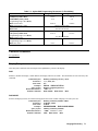
OPERATING GUIDE for
SOLAR ARRAY SIMULATOR
AGILENT MODELS E4350B, E4351B
Agilent Part No. 5962-8206
Microfiche 5962-8207
Printed in Malaysia
September, 2004
CERTIFICATION
Agilent Technologies Company certifies that this product met its published specifications at time of shipment from the
factory. Agilent Technologies further certifies that its calibration measurements are traceable to the United States National
Bureau of Standards, to the extent allowed by the Bureau's calibration facility, and to the calibration facilities of other
International Standards Organization members.
WARRANTY
This Agilent Technologies hardware product is warranted against defects in material and workmanship for a period of one
year from date of delivery. Agilent software and firmware products, which are designated by Agilent for use with a
hardware product and when properly installed on that hardware product, are warranted not to fail to execute their
programming instructions due to defects in material and workmanship for a period of 90 days from date of delivery. During
the warranty period Agilent Technologies Company will, at its option, either repair or replace products which prove to be
defective. Agilent does not warrant that the operation of the software, firmware, or hardware shall be uninterrupted or error
free.
For warranty service, with the exception of warranty options, this product must be returned to a service facility designated
by Agilent. Customer shall prepay shipping charges by (and shall pay all duty and taxes) for products returned to Agilent for
warranty service. Except for products returned to Customer from another country, Agilent shall pay for return of products to
Customer.
Warranty services outside the country of initial purchase are included in Agilent's product price, only if Customer pays
Agilent international prices (defined as destination local currency price, or U.S. or Geneva Export price).
If Agilent is unable, within a reasonable time to repair or replace any product to condition as warranted, the Customer shall
be entitled to a refund of the purchase price upon return of the product to Agilent.
LIMITATION OF WARRANTY
The foregoing warranty shall not apply to defects resulting from improper or inadequate maintenance by the Customer,
Customer-supplied software or interfacing, unauthorized modification or misuse, operation outside of the environmental
specifications for the product, or improper site preparation and maintenance. NO OTHER WARRANTY IS EXPRESSED
OR IMPLIED. AGILENT SPECIFICALLY DISCLAIMS THE IMPLIED WARRANTIES OF MERCHANTABILITY
AND FITNESS FOR A PARTICULAR PURPOSE.
EXCLUSIVE REMEDIES
THE REMEDIES PROVIDED HEREIN ARE THE CUSTOMER'S SOLE AND EXCLUSIVE REMEDIES. AGILENT
SHALL NOT BE LIABLE FOR ANY DIRECT, INDIRECT, SPECIAL, INCIDENTAL, OR CONSEQUENTIAL
DAMAGES, WHETHER BASED ON CONTRACT, TORT, OR ANY OTHER LEGAL THEORY.
ASSISTANCE
The above statements apply only to the standard product warranty. Warranty options, extended support contracts, product
maintenance agreements and customer assistance agreements are also available. Contact your nearest Agilent
Technologies Sales and Service office for further information on Agilent's full line of Support Programs.
2
Safety Summary
The following general safety precautions must be observed during all phases of operation, service, and repair of this
instrument. Failure to comply with these precautions or with specific warnings elsewhere in this manual violates safety
standards of design, manufacture, and intended use of the instrument. Agilent Technologies Company assumes no liability
for the customer’s failure to comply with these requirements.
GENERAL.
This product is a Safety Class 1 instrument (provided with a protective earth terminal).
Any LEDs used in this product are Class 1 LEDs as per IEC 825-l.
This ISM device complies with Canadian ICES-001. Cet appareil ISM est conforme à la norme NMB-001 du Canada.
ENVIRONMENTAL CONDITIONS
With the exceptions noted, all instruments are intended for indoor use in an installation category II, pollution degree 2 environment.
They are designed to operate at a maximum relative humidity of 95% and at altitudes of up to 2000 meters. Refer to the specifications
tables for the ac mains voltage requirements and ambient operating temperature range.
BEFORE APPLYING POWER.
Verify that the product is set to match the available line voltage and the correct fuse is installed.
GROUND THE INSTRUMENT.
To minimize shock hazard, the instrument chassis and cabinet must be connected to an electrical ground. The instrument must be
connected to the ac power supply mains through a three-conductor power cable, with the third wire firmly connected to an electrical
ground (safety ground) at the power outlet. For instruments designed to be hard-wired to the ac power lines (supply mains), connect the
protective earth terminal to a protective conductor before any other connection is made. Any interruption of the protective (grounding)
conductor or disconnection of the protective earth terminal will cause a potential shock hazard that could result in personal injury. If the
instrument is to be energized via an external autotransformer for voltage reduction, be certain that the autotransformer common terminal
is connected to the neutral (earthed pole) of the ac power lines (supply mains).
FUSES.
Only fuses with the required rated current, voltage, and specified type (normal blow, time delay, etc.) should be used. Do not use repaired
fuses or short circuited fuseholders. To do so could cause a shock or fire hazard.
DO NOT OPERATE IN AN EXPLOSIVE ATMOSPHERE.
Do not operate the instrument in the presence of flammable gases or fumes.
KEEP AWAY FROM LIVE CIRCUITS.
Operating personnel must not remove instrument covers. Component replacement and internal adjustments must be made by qualified
service personnel. Do not replace components with power cable connected. Under certain conditions, dangerous voltages may exist even
with the power cable removed. To avoid injuries, always disconnect power, discharge circuits and remove external voltage sources before
touching components.
DO NOT SERVICE OR ADJUST ALONE.
Do not attempt internal service or adjustment unless another person, capable of rendering first aid and resuscitation, is present.
DO NOT EXCEED INPUT RATINGS.
This instrument may be equipped with a line filter to reduce electromagnetic interference and must be connected to a properly grounded
receptacle to minimize electric shock hazard. Operation at line voltages or frequencies in excess of those stated on the data plate may
cause leakage currents in excess of 5.0 mA peak.
DO NOT SUBSTITUTE PARTS OR MODIFY INSTRUMENT.
Because of the danger of introducing additional hazards, do not install substitute parts or perform any unauthorized modification to the
instrument. Return the instrument to an Agilent Technologies Sales and Service Office for service and repair to ensure that safety features
are maintained.
Instruments which appear damaged or defective should be made inoperative and secured against unintended operation until they can be
repaired by qualified service personnel.
3
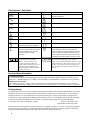
Safety Symbol - Definitions
Symbol
Description
Direct current
Symbol
Alternating current
Description
Terminal for Line conductor on permanently
installed equipment
Caution, risk of electric shock
Both direct and alternating current
Caution, hot surface
Three-phase alternating current
Caution (refer to accompanying documents)
Earth (ground) terminal
In position of a bi-stable push control
Protective earth (ground) terminal
Out position of a bi-stable push control
Frame or chassis terminal
On (unit)
Terminal for Neutral conductor on
permanently installed equipment
Terminal is at earth potential
(Used for measurement and control
circuits designed to be operated
with one terminal at earth
potential.)
Off (unit)
The WARNING sign denotes a hazard.
It calls attention to a procedure,
practice, or the like, which, if not
correctly performed or adhered to,
could result in personal injury. Do not
proceed beyond a WARNING sign
until the indicated conditions are fully
understood and met.
The CAUTION sign denotes a hazard. It calls
attention to an operating procedure, or the like,
which, if not correctly performed or adhered to, could
result in damage to or destruction of part or all of the
product. Do not proceed beyond a CAUTION sign
until the indicated conditions are fully understood
and met.
Standby (unit)
Units with this symbol are not completely
disconnected from ac mains when this switch is
off. To completely disconnect the unit from ac
mains, either disconnect the power cord or have
a qualified electrician install an external switch.
Acoustic Noise Information
Herstellerbescheinigung
Diese Information steht im Zusammenhang mit den Anforderungen der Maschinenläminformationsverordnung vom 18
Januar 1991. * Schalldruckpegel Lp <70 dB(A) * Am Arbeitsplatz * Normaler Betrieb * Nach EN 27779 (Typprufung).
Manufacturer's Declaration
This statement is provided to comply with the requirements of the German Sound Emission Directive, from 18 January
1991. * Sound Pressure Lp <70 dB(A) *At Operator Position * Normal Operation * According to EN 27779 (Type Test).
Printing History
The edition and current revision of this manual are indicated below. Reprints of this manual containing minor corrections
and updates may have the same printing date. Revised editions are identified by a new printing date. A revised edition
incorporates all new or corrected material since the previous printing date. Changes to the manual occurring between
revisions are covered by change sheets shipped with the manual. In some cases, the changes apply to specific instruments.
Instructions provided on the change sheet will indicate if a particular change applies only to certain instruments.
Copyright 1997 Agilent Technologies Company
Edition 1 - December, 1997
Updated: March, 2000; Sept. 2004
This document contains proprietary information protected by copyright. All rights are reserved. No part of this document
may be photocopied, reproduced, or translated into another language without the prior consent of Agilent Technologies
Company. The information contained in this document is subject to change without notice.
4
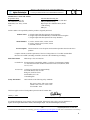
DECLARATION OF CONFORMITY
According to ISO/IEC Guide 22 and CEN/CENELEC EN 45014
Manufacturer’s Name and Address
Responsible Party
Agilent Technologies, Inc.
550 Clark Drive, Suite 101
Budd Lake, New Jersey 07828
USA
Alternate Manufacturing Site
Agilent Technologies (Malaysia) Sdn. Bhd
Malaysia Manufacturing
Bayan Lepas Free Industrial Zone, PH III
11900 Penang,
Malaysia
Declares under sole responsibility that the product as originally delivered
Product Names
a) Single Output 500 Watt System dc Power Supplies
b) Single Output 500 Watt Manually Controlled dc Power Supplies
c) Single Output 500 Watt System Solar Array Simulator
Model Numbers
a) 6651A, 6652A 6653A, 6654A, 6655A
b) 6551A, 6552A 6553A, 6554A, 6555A
c) E4350B, E4351B
Product Options
This declaration covers all options and customized products based on the above
products.
Complies with the essential requirements of the Low Voltage Directive 73/23/EEC and the EMC
Directive 89/336/EEC (including 93/68/EEC) and carries the CE Marking accordingly.
EMC Information
As detailed in
Assessed by:
Safety Information
ISM Group 1 Class A Emissions
Electromagnetic Compatibility (EMC), Certificate of Conformance Number
CC/TCF/00/074 based on Technical Construction File (TCF) HPNJ1, dated
Oct. 27, 1997
Celestica Ltd, Appointed Competent Body
Westfields House, West Avenue
Kidsgrove, Stoke-on-Trent
Straffordshire, ST7 1TL
United Kingdom
and Conforms to the following safety standards.
IEC 61010-1:2001 / EN 61010-1:2001
Canada: CSA C22.2 No. 1010.1:1992
UL 61010B-1: 2003
This DoC applies to above-listed products placed on the EU market after:
January 1, 2004
Date
Bill Darcy/ Regulations Manager
For further information, please contact your local Agilent Technologies sales office, agent or distributor, or
Agilent Technologies Deutschland GmbH, Herrenberger Straβe 130, D71034 Böblingen, Germany
Revision: B.00.00
Issue Date: Created on 11/24/2003 3:26
PM
Document No.
6x4yA6x5yAE435xA.b.11.24doc.doc
To obtain the latest Declaration of Conformity, go to http://regulations.corporate.agilent.com and click on “Declarations of Conformity.”
5
Table Of Contents
1
General Information
What’s In This Guide? ..................................................................................................................................13
Safety Considerations....................................................................................................................................13
Options and Accessories................................................................................................................................13
Operator Replaceable Parts ...........................................................................................................................14
Description ....................................................................................................................................................14
Key Features..................................................................................................................................................14
Output Characteristic.....................................................................................................................................15
Fixed Mode .............................................................................................................................................15
Simulator Mode.......................................................................................................................................15
Table Mode .............................................................................................................................................17
2
Installation
Inspection ......................................................................................................................................................19
Damage....................................................................................................................................................19
Packaging Material..................................................................................................................................19
Items Supplied.........................................................................................................................................19
Location and Temperature.............................................................................................................................19
Bench Operation......................................................................................................................................19
Rack Mounting ........................................................................................................................................20
Temperature Performance .......................................................................................................................20
AC Line Connection......................................................................................................................................20
AC Voltage Conversion ................................................................................................................................21
VXI plug&play Power Products Instrument Drivers.....................................................................................21
Downloading and Installing the Driver ...................................................................................................22
Accessing Online Help ............................................................................................................................22
3
Turn-on Checkout
Introduction ...................................................................................................................................................23
Preliminary Checkout ....................................................................................................................................23
Power-on Checkout .......................................................................................................................................23
Using the Keypad ..........................................................................................................................................24
Shifted Keys ............................................................................................................................................24
Backspace Key ........................................................................................................................................24
Output Checkout............................................................................................................................................24
Checking the Voltage Function ...............................................................................................................24
Checking the Current Function................................................................................................................25
Checking the Save and Recall Functions.......................................................................................................27
Determining GPIB Address...........................................................................................................................27
In Case of Trouble.........................................................................................................................................27
Line Fuse .................................................................................................................................................27
Error Messages........................................................................................................................................27
Selftest Errors..........................................................................................................................................27
Power-On Error Messages.......................................................................................................................27
Checksum Errors .....................................................................................................................................28
Runtime Error Messages .........................................................................................................................28
4
User Connections
Rear Panel Connections.................................................................................................................................29
Wire Selection .........................................................................................................................................29
Analog Connector....................................................................................................................................29
Digital Connector ....................................................................................................................................30
Load Connections..........................................................................................................................................30
Output Isolation.......................................................................................................................................30
6
Capacitive Loads .....................................................................................................................................30
Inductive Loads ......................................................................................................................................31
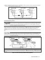
Connecting to an External Voltage Source..............................................................................................31
Sense Connections.........................................................................................................................................31
Remote Voltage Sensing .........................................................................................................................31
CV Regulation.........................................................................................................................................32
Overvoltage Protection Considerations ...................................................................................................32
Output Rating ..........................................................................................................................................32
Output Noise ...........................................................................................................................................32
Stability ...................................................................................................................................................32
Over Current Protection Considerations........................................................................................................33
Hardware Overcurrent Circuit .................................................................................................................33
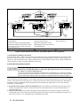
Operating Configurations ..............................................................................................................................33
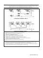
Connecting the Load to One Unit ...........................................................................................................33
Connecting Supplies in Parallel...............................................................................................................34
Connecting Supplies in Auto-Parallel......................................................................................................35
Auto-Parallel Programming Cautions......................................................................................................36
Connecting Supplies in Series .................................................................................................................37
Analog Current Control...........................................................................................................................38
Controller Connections..................................................................................................................................38
Stand-Alone Connections ........................................................................................................................38
Linked Connections.................................................................................................................................38
5
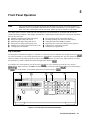
Front Panel Operation
Introduction ...................................................................................................................................................41
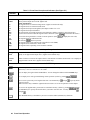
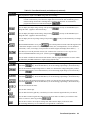
Key Functions................................................................................................................................................41
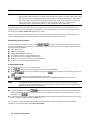
Programming the Output .........................................................................................................................44
Establishing Initial Conditions. ...............................................................................................................44
Programming Voltage .............................................................................................................................44
Programming Current. .............................................................................................................................45
Programming Overvoltage Protection ...........................................................................................................45
Setting the OVP Level..............................................................................................................................45
Checking OVP Operation.........................................................................................................................45
Clearing the OVP Condition ....................................................................................................................46
Programming Overcurrent Protection............................................................................................................46
Setting the OCP Protection.......................................................................................................................46
Checking OCP Operation .........................................................................................................................46
Clearing the OCP Condition.....................................................................................................................46
CV Mode vs. CC Mode.................................................................................................................................47
Unregulated Operation ..................................................................................................................................47
Saving and Recalling States ..........................................................................................................................47
Turn-on Conditions .......................................................................................................................................47
Setting the GPIB Address..............................................................................................................................48
Types of GPIB Addresses .......................................................................................................................48
Changing the GPIB Address....................................................................................................................48
6.
Remote Programming
GPIB Capabilities of the Power Supply ........................................................................................................49
Introduction to SCPI......................................................................................................................................49
Conventions.............................................................................................................................................49
Types of SCPI Commands ............................................................................................................................50
Multiple Commands in a Message...........................................................................................................50
Moving Among Subsystems ....................................................................................................................51
Value Coupling........................................................................................................................................51
Including Common Commands ...............................................................................................................51
SCPI Queries ...........................................................................................................................................51
7
Types of SCPI Messages ..............................................................................................................................51
The Message Unit....................................................................................................................................52
Headers....................................................................................................................................................52
Query Indicator .......................................................................................................................................52
Message Unit Separator...........................................................................................................................52
Root Specifier..........................................................................................................................................52
Message Terminator ................................................................................................................................52
SCPI Data Formats........................................................................................................................................53
Numerical Data........................................................................................................................................53
Suffixes and Multipliers ..........................................................................................................................53
Character Data.........................................................................................................................................53
Examples .......................................................................................................................................................54
Programming Voltage and Current..........................................................................................................54
Programming Protection Circuits ............................................................................................................54
Programming Units in Auto-Parallel .......................................................................................................54
Changing Outputs by Trigger ..................................................................................................................55
Saving and Recalling States ....................................................................................................................55
Writing to the Display .............................................................................................................................56
Programming Status ................................................................................................................................56
Programming the Digital I/O Port ...........................................................................................................56
System Considerations ..................................................................................................................................56
Assigning GPIB Address in Programs.....................................................................................................57
Agilent 82335A Driver Considerations ...................................................................................................57
National Instruments GPIB Driver Considerations .................................................................................57
BASIC Considerations ............................................................................................................................57
7.
Language Dictionary
Introduction ...................................................................................................................................................61
Parameters ...............................................................................................................................................61
Related Commands..................................................................................................................................61
Order of Presentation ..............................................................................................................................61
Common Commands ...............................................................................................................................61
Subsystem Commands.............................................................................................................................61
Description of Common Commands .............................................................................................................62
*CLS........................................................................................................................................................62
*ESE........................................................................................................................................................62
*ESR?......................................................................................................................................................63
*IDN?......................................................................................................................................................63
*OPC .......................................................................................................................................................64
*OPC? .....................................................................................................................................................64
*OPT? .....................................................................................................................................................64
*PSC........................................................................................................................................................65
*RCL .......................................................................................................................................................65
*RST .......................................................................................................................................................66
*SAV.......................................................................................................................................................66
*SRE .......................................................................................................................................................67
*STB?......................................................................................................................................................67
*TRG.......................................................................................................................................................68
*TST?......................................................................................................................................................68
*WAI.......................................................................................................................................................68
Description of Subsystem Commands ...........................................................................................................69
Calibration Commands ..................................................................................................................................71
Display Subsystem ........................................................................................................................................71
DISP ........................................................................................................................................................71
DISP:MODE ...........................................................................................................................................71
DISP:TEXT.............................................................................................................................................72
8
Measure Subsystem .......................................................................................................................................72
MEAS:CURR? ........................................................................................................................................72
MEAS:VOLT? ........................................................................................................................................72
Memory Subsystem .......................................................................................................................................73
MEM:COPY:TABL ................................................................................................................................73
MEM:DEL:ALL......................................................................................................................................73
MEM:DEL[:NAME] ...............................................................................................................................73
MEM:TABL:SEL....................................................................................................................................73
MEM:TABL:CURR................................................................................................................................73
MEM:TABL:VOLT ................................................................................................................................73
MEM:TABL:CURR:POIN?....................................................................................................................74
MEM:TABL:VOLT:POIN?....................................................................................................................74
MEM:TABL:CAT? .................................................................................................................................74
Output Subsystem..........................................................................................................................................74
OUTP ......................................................................................................................................................74
OUTP:PROT:CLE ..................................................................................................................................74
OUTP:PROT:DEL ..................................................................................................................................75
[SOUR:]CURR........................................................................................................................................75
[SOUR:]CURR:TRIG .............................................................................................................................75
[SOUR:]CURR:MODE...........................................................................................................................76
[SOUR:]CURR:PROT ............................................................................................................................76
[SOUR:]CURR:PROT:STAT .................................................................................................................76
[SOUR:]CURR:SAS:ISC ........................................................................................................................77
[SOUR:]CURR:SAS:IMP .......................................................................................................................77
[SOUR:]CURR:TABL:NAME ...............................................................................................................77
[SOUR:]CURR:TABL:OFFS..................................................................................................................77
[SOUR:]DIG:DATA ...............................................................................................................................77
[SOUR:]VOLT........................................................................................................................................78
[SOUR:]VOLT:TRIG .............................................................................................................................78
[SOUR:]VOLT:PROT ............................................................................................................................79
[SOUR:]VOLT:SAS:VOC ......................................................................................................................79
[SOUR:]VOLT:SAS:VMP......................................................................................................................79
[SOUR:]VOLT:TABL:OFFS..................................................................................................................80
Status Subsystem ...........................................................................................................................................80
STAT:OPER?..........................................................................................................................................80
STAT:OPER:COND? .............................................................................................................................80
STAT:OPER:ENAB................................................................................................................................81
STAT:OPER:PTR/NTR ..........................................................................................................................81
STAT:PRES ............................................................................................................................................81
STAT:QUES? .........................................................................................................................................82
STAT:QUES:COND? .............................................................................................................................82
STAT:QUES:ENAB ...............................................................................................................................82
STAT:QUES:PTR/NTR..........................................................................................................................83
System Commands ........................................................................................................................................83
SYST:ERR? ............................................................................................................................................83
SYST:VERS? ..........................................................................................................................................84
Trigger Subsystem.........................................................................................................................................84
ABOR......................................................................................................................................................84
INIT84
INIT:CONT.............................................................................................................................................84
TRIG .......................................................................................................................................................85
TRIG:SOUR............................................................................................................................................85
9
8.
Status Reporting
Agilent SAS Status Structure.........................................................................................................................87
Operation Status Group .................................................................................................................................87
Register Functions ...................................................................................................................................87
Register Commands.................................................................................................................................87
Questionable Status Group ............................................................................................................................89
Register Functions ...................................................................................................................................89
Register Commands.................................................................................................................................89
Standard Event Status Group.........................................................................................................................89
Register Functions ...................................................................................................................................89
Register Commands.................................................................................................................................89
Status Byte Register ......................................................................................................................................89
The RQS Bit............................................................................................................................................90
The MSS Bit............................................................................................................................................90
Determining the Cause of a Service Interrupt..........................................................................................90
Service Request Enable Register ...................................................................................................................90
Output Queue ................................................................................................................................................90
Initial Conditions at Power-On......................................................................................................................90
Status Registers .......................................................................................................................................90
The PON (Power-On) Bit........................................................................................................................91
Examples .......................................................................................................................................................91
Servicing an Operation Status Mode Event.............................................................................................91
Adding More Operation Events...............................................................................................................91
Servicing Questionable Status Events .....................................................................................................91
Monitoring Both Phases of a Status Transition .......................................................................................92
SCPI Command Completion .........................................................................................................................92
DFI (Discrete Fault Indicator) .......................................................................................................................92
RI (Remote Inhibit) .......................................................................................................................................93
Using Device Clear .......................................................................................................................................93
A
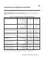
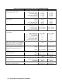
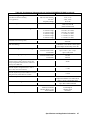
Specifications and Application Information
Specifications and Supplemental Characteristics ..........................................................................................95
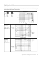
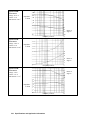
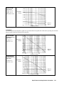
Output Impedance Graphs.............................................................................................................................99
Simulator Mode.......................................................................................................................................99
Fixed Mode ...........................................................................................................................................101
Peak Power Tracker Application ................................................................................................................102
Exponential Model Equations ...............................................................................................................103
Series Switching Regulation........................................................................................................................104
Shunt Switching Regulation ........................................................................................................................104
B
Verification and Calibration
Introduction .................................................................................................................................................105
Test Equipment Required ............................................................................................................................105
Current Monitoring Resistor..................................................................................................................105
Verification..................................................................................................................................................106
General Measurement Techniques ........................................................................................................106
Programming the Agilent SAS ..............................................................................................................106
Order of Tests........................................................................................................................................106
Turn On Checkout .................................................................................................................................106
Voltage Programming and Readback Accuracy ....................................................................................106
Current Programming and Readback Accuracy.....................................................................................107
Calibration...................................................................................................................................................108
Test Equipment Required ......................................................................................................................108
General Procedure .................................................................................................................................108
Parameters Calibrated............................................................................................................................108
Front Panel Calibration ...............................................................................................................................109
10
Entering the Calibration Values ............................................................................................................109
Saving the Calibration Constants...........................................................................................................109
Disabling the Calibration Mode ............................................................................................................109
Changing the Calibration Password.......................................................................................................109
Recovering From Calibration Problems ................................................................................................111
Calibration Error Messages ...................................................................................................................111
Calibration over the GPIB...........................................................................................................................111
Calibration Example..............................................................................................................................111
Calibration Language Dictionary ................................................................................................................112
CAL:CURR ...........................................................................................................................................112
CAL:CURR:LEV ..................................................................................................................................112
CAL:PASS ............................................................................................................................................112
CAL:SAVE ...........................................................................................................................................112
CAL:STAT............................................................................................................................................113
CAL:VOLT ...........................................................................................................................................113
CAL:VOLT:LEV ..................................................................................................................................113
CAL:VOLT:PROT ................................................................................................................................113
Agilent Basic Calibration Program..............................................................................................................114
C
Digital Port Functions
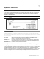
Digital Connector ........................................................................................................................................117
Fault/Inhibit Operation ................................................................................................................................117
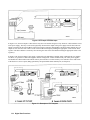
Changing the Port Configuration.................................................................................................................119
Digital I/O Operation...................................................................................................................................119
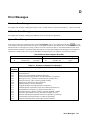
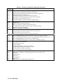
D
Error Messages
Hardware Error Messages ...........................................................................................................................121
Calibration Error Messages .........................................................................................................................121
System Error Messages ...............................................................................................................................121
Index ..........................................................................................................................................................123
Agilent Sales and Support Offices .....................................................................................................128
11
1
General Information
What’s In This Guide?
This guide describes the Agilent Model E4350B/E4351B Solar Array Simulator (SAS). An overview of the unit is given in
this chapter. Installation and user connections are discussed in chapters 2 and 4. Programming from the front panel and over
the GPIB is discussed in chapters 5-7. If you just need to check that the unit is operating properly, read chapter 3.
The edition and current revision of this manual are indicated on the title page. Reprints of this manual containing minor
corrections and updates may have the same printing date. Revised editions are identified by a new printing date. A revised
edition incorporates all new or corrected material since the previous printing date.
Changes to the manual occurring between revisions are covered by change sheets shipped with the manual. In some cases,
the manual change applies only to specific instruments. Instructions provided on the change sheet will indicate if a particular
change applies only to certain instruments.
Safety Considerations
The Agilent Solar Array Simulator is a Safety Class 1 instrument, which means it has a protective earth terminal. That
terminal must be connected to earth ground through a power source equipped with a 3-wire ground receptacle. Refer to the
Safety Summary page at the beginning of this guide for general safety information. Before installation or operation, check
the Agilent SAS and review this guide for safety warnings and instructions. Safety warnings for specific procedures are
located at appropriate places in the guide.
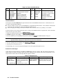
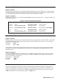
Options and Accessories
Option
100
220
240
909
0B3
Table 1-1 Options
Description
Input power 100 Vac, nominal
Input power 220 Vac, nominal
Input power 240 Vac, nominal (for 230 Vac operation, see table A-2 in appendix A)
Rack mount kit (Agilent 5062-3977) Support rails (E3663A) are required.
Rack mount kit (Agilent 5062-3977 & 5062-3974) Support rails (E3663A) are required.
Rack mount kit with handles (Agilent 5062-3983) Support rails (E3663A) are required.
Service manual
Table 1-2 Accessories
Accessory Description
GPIB cable (all models)
0.5 meters (1.6 ft)
1.0 meter (3.3 ft)
2.0 meters (6.6 ft)
4.0 meters ( 13 .2 ft)
Serial link cable (all models)
2.0 meters (6.6 ft)
Slide mount kit
Agilent No.
10833D
10833A
10833B
10833C
5080-2148
1494-0059
General Information
13
Operator Replaceable Parts
Description
Cover, dc output
Foot, cabinet
Fuse, power
100 Vac line voltage, 15 A
120 Vac line voltage, 12 A
220/230/240 Vac line voltage, 7 A
Knob, rotary output control
Table 1-3 Operator Replaceable Parts
Agilent Part No.
Description
0360-2191
Plug, analog connector
5041-8801
Plug, digital connector
Screw, output bus bar
Screw, terminal cover
2110-0054
Screw, carrying strap, M5x0.8x10 mm
2110-0249
Standoff, GPIB
21l0-06l4
0370-3238
Agilent Part No.
1252-3698
1252-1488
0515-1085
0515-1085
0515-1132
0380-0644
Description
The Agilent E4350B/E4351B Solar Array Simulator (SAS) is a dc power source that simulates the output characteristics of
a solar array. The Agilent SAS is primarily a current source with very low output capacitance. It is capable of simulating the
I-V curve of a solar array under different conditions such as temperature and age. The I-V curve is programmable over the
IEEE-488.2 bus and is automatically generated within the Agilent SAS. The Agilent SAS has three operating modes:
Fixed Mode: This is the default mode that occurs when the unit is first powered up. The I-V output has the rectangular
characteristics of a standard power supply, but with excellent high speed constant current characteristics and low output
capacitance. Fixed mode allows front panel programming and is convenient when, in certain applications, the I-V curve is
not needed.
Simulator Mode: An internal algorithm is used to simulate a SAS I-V curve. One can easily approximate the curve through
four input parameters: open circuit voltage (Voc), short circuit current (Isc), current at the approximate maximum power
point on the curve (Imp), and voltage at the approximate maximum power point on the curve (Vmp).
Table Mode: The Agilent SAS provides a table mode for a fast and accurate I-V simulation of solar arrays. In this mode, a
table of I-V points, often provided by the solar array manufacturer, specifies the curve. The Agilent SAS provides up to 60
tables with a total of 33,500 I-V points of storage and a maximum of 4,000 I-V points per table. The tables (I-V curves) are
easily stored and recalled. A portion of table storage is allocated in non-volatile memory, with 30 possible tables totaling
3,500 points. These are retained when power is turned off. In table mode, current and voltage offsets can be applied to the
selected table to simulate a change in the operating conditions of the solar array.
Key Features
■
■
■
■
■
■
■
■
■
■
■
■
■
480 Watt output
Auto-parallel capability for higher power
Very low output capacitance
Switching recovery time in less than 5 microseconds
Programmable overvoltage and over-current protection which are independent of other circuits
Overtemperature protection
Fan speed control to minimize acoustic noise
Extensive set of programming features
Fast I-V curve change in both table and simulator modes
Up to 60 volatile/non-volatile tables
Self test at power-up or from an IEEE-488.2 command
Serial link to connect up to 16 outputs to one IEEE-488.2 address
Standard Commands for Programmable Instruments (SCPI)
14
General Information
Output Characteristic
The Agilent E4350B/E4351B Solar Array Simulator can be operated in three modes: fixed mode, simulator mode, and table
mode. Mode switching on the Agilent SAS is accomplished over the GPIB bus via the SCPI CURRent:MODE command.
You cannot switch modes from the front panel.
Note:
The Agilent SAS must be connected to a computer for you to be able to use the SAS functions that are
available in simulator and table modes.
The front panel does not indicate which mode the Agilent SAS is presently operating in. If you are unsure which mode the
unit is presently in, you can query the unit over the GPIB using the CURRent:MODE? command. If you cycle power to the
unit, it will be in Fixed mode.
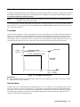
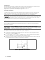
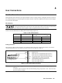
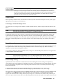
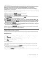
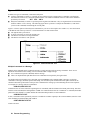
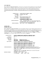
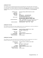
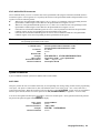
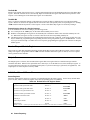
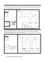
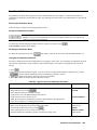
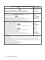
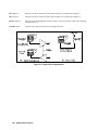
Fixed Mode
At power turn on, with *RST, or when executing a Device Clear, the operating state of the Agilent SAS is Fixed mode (see
Figure 1-1). In Fixed mode, the output characteristic is similar to that of a standard power supply, except that the output
capacitance is <100 nF on the Agilent E4350B, and <50 nF on the Agilent E4351B. This low output capacitance is ideal
when using the unit as a constant current source. To use the unit as a low-impedance constant voltage source however, you
can add an external output capacitor if so desired. The value of the external capacitor should not exceed 2,000 µF.
I
I
480W MAX
MAXIMUM CURRENT
E4351B = 4A
E4350B = 8A
TYPICAL FIXED MODE OUTPUT
set
MAXIMUM
VOLTAGE
0
V
V
set
120V = E4351B
60V = E4350B
Figure 1-1. Fixed Mode Characteristic
Restrictions
■ If the programmed values exceed the maximum current and voltage boundaries by more than 2 or 3 percent, an OUT
OF RANGE error will be indicated.
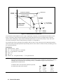
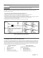
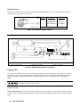
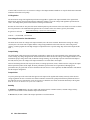
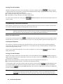
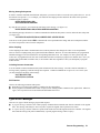
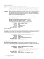
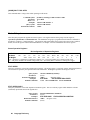
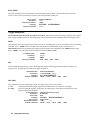
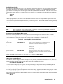
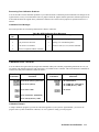
Simulator Mode
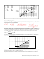
Simulator mode uses an exponential model to approximate the I-V curve (see Figure 1-2). It is programmed in terms of its
open circuit voltage (Voc), short circuit current (Isc), voltage point (Vmp), and current point (Imp) at approximately the
peak power point (see page A-9 in appendix A for model equations). Simulator mode operation is achieved by sampling
the output voltage, applying a low-pass filter, and continually adjusting the constant current loop by using the filtered
voltage as an index into the exponential model.
General Information
15
I
I
480W MAX
MAXIMUM CURRENT
E4351B = 4A
E4350B = 8A
I
sc
P
mp
TYPICAL CURVE
MAXIMUM
VOLTAGE
mp
V
I
POINTS UNDER
DASHED LINE
ARE INVALID
0
Vmp
= 1Ω min (E4351B)
.25Ω min (E4350B)
V
Voc
120V
60V
130V = E4351B
65V = E4350B
Figure 1-2. Simulator Mode Characteristic
Note that under certain conditions, such as if Imp is significantly less than Isc, the model equation will exhibit a certain
degree of inaccuracy in that the actual maximum power point (Pmp) and value may be somewhat different from the
expected value of Pmp (Imp x Vmp). Thus the actual Pmp point may not occur at exactly the Imp x Vmp. This can be
corrected by entering new values for Imp and Vmp (see Figure A-1 in appendix A).
Also note that the accuracy specifications in simulator mode are relative to the values given in the exponential equations,
and not necessarily to the input parameters Imp and Vmp. However, the Isc and Voc values are always accurately given by
the exponential equations.
Restrictions:
Maximum Power ≤ 480 W
■ Voc ≤ 130 V (E4351B) or 65 V (E4350B)
■ Isc ≤ 4 A (E4351B) or 8 A (E4350B)
■ Vmp < Voc
■ Imp ≤ Isc
■ ∆V/∆I ≥ .25 Ω for Agilent E4350B; ≥ 1 Ω for Agilent E4351B
■
NOTE:
When the unit detects invalid equation parameters, it will generate an error, light the ERR annunciator on the
front panel, and will not use the new parameters. Instead, it will operate with the last valid settings. Therefore,
although it may seem that the unit is operating correctly, it will NOT be using the values that you have
programmed for simulator mode.
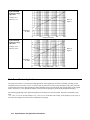
If simulator mode is entered with no parameters specified,
the default values that will be used are:
16
General Information
Voc
Vmp
Imp
Isc
Pmp
E4350B
61.5 V
49.2 V
6.528 A
8.16 A
321.2 W
E4351B
123 V
98.4 V
3.264 A
4.08 A
321.2 W
Front panel operation:
You can use the front panel when the unit is operating in Simulator mode. To do this, press the Local key whenever the
front panel RMT annunciator is on. Be aware however, that any voltage and current values that you enter from the front
panel will have no effect on the unit while it is in Simulator mode. These front panel values will take effect as soon as the
unit is placed in Fixed mode. Likewise, the OCP function only takes effect in Fixed mode. All other functions such as Local,
Error, Output On/Off, Protect are active while the unit is operating in Simulator mode.
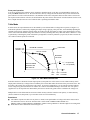
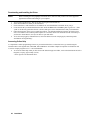
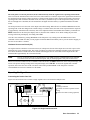
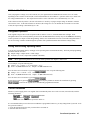
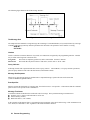
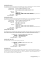
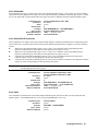
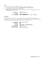
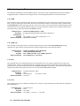
Table Mode
In Table mode, the output characteristic is determined by a user-defined table of voltage/current points (see Figure 1-3).
Table mode operation is achieved by sampling the output voltage, applying a low-pass filter, and continually adjusting the
constant current loop by using the filtered voltage as an index into the stored table of points. Linear interpolation is used to
set the current when the filtered voltage does not have an exactly matching table entry. What this means is that the I-V curve
is generated by connecting the points in the table by straight lines. The more points that you provide, the more accurate the
curve will be when the points are connected.
I
480W MAX
MAXIMUM CURRENT
E4351B = 4A
E4350B = 8A
I
sc
TYPICAL CURVE
MAXIMUM
VOLTAGE
V
I
POINTS UNDER
DASHED LINE
ARE INVALID
0
V oc
= 1Ω min (E4351B)
.25Ω min (E4350B)
V
120V
60V
130V = E4351B
65V = E4350B
Figure 1-3. Table Mode Characteristic
Each table can have a maximum of 4,000 output points (3,500 points if it will be stored in non-volatile memory). Each
output point is defined by a voltage/current coordinate pair of values that define the location of the point on the curve. The
first value is the voltage, the second value is the current. If no point is supplied for V=0, the current associated with the
lowest voltage entry point is defined as Isc and the curve will be extended horizontally to the current axis. If no point is
supplied for I=0, the slope that was determined by the last two current entry points will be extended to the voltage axis.
Multiple tables can be defined and saved in non-volatile memory (which is limited to 3500 points), or volatile memory
(which is limited to 30,000 points). Up to 30 tables can be saved in each memory.
Restrictions
■ The number of points in a table can vary from 3 to 4000, but an equal number of voltage and current values must be
sent. Otherwise an error will occur when the table is selected with CURRent:TABLe:NAME. Use
MEMory:TABLe:CURRent:POINts? and MEMory:TABLe:VOLTage:POINts? to find the length of an existing table.
■ Points must be above dashed line shown in Figure 1-3.
General Information
17
■
■
■
■
■
There is no restriction on the spacing between points in either voltage or current, but the points must be monotonic.
Voltage values must be sent in increasing order of magnitude; current values must be sent in equal or decreasing order
of magnitude. For an Agilent E4350B for example: (1,8) (50,7.8) (55,7.5) (56,7) (57, 6) (58, 4) (59,1).
Each table point, when combined with the table offset, cannot exceed the unit’s maximum voltage, current, or power.
A table cannot be deleted or redefined while it is selected with CURRent:TABLe:NAME.
Maximum Power ≤ 480 W
∆V/∆I ≥ .25 Ω for Agilent E4350B; ≥ 1 Ω for Agilent E4351B
Voc ≤ 65V (Agilent E4350B); 130V (Agilent E4351B)
Isc ≤ 8A (Agilent E4350B); 4A (Agilent E4351B)
The Vmp and Imp points are calculated internally and need not be supplied.
NOTE:
When the unit detects an invalid voltage/current point, it will generate an error, light the ERR annunciator on
the front panel, and will not use the new parameters. Instead, it will operate with the last valid table settings.
Therefore, although it may seem that the unit is operating correctly, it will NOT be using the values that you
have programmed for table mode.
Table Offsets:
A new table can be generated by applying a limited voltage or current offset to an existing table. This can be helpful in
simulating temperature, angular, rotational, or aging changes. Offset values are non-cumulative, they can be either positive
or negative, and can be applied to any table. Each time a voltage or current offset is programmed, a new I-V curve is
calculated based on the user-defined table that is presently active and the supplied offset values. Offset values affect the
original I-V curve as follows:
Positive Voltage Offsets:
The original curve is shifted to the right (È) along the positive voltage axis, and the first
point on the curve is extended horizontally at Isc until it intersects the current axis. Thus,
the new Voc equals the original Voc plus the offset value. An error will be generated if the
offset causes the maximum allowed Voc or the power limit to be exceeded.
Negative Voltage Offsets:
The original curve is offset to the left (Ç) along the positive voltage axis, and terminated at
the current axis. The curve points that are not used because they extended beyond the
current axis are not deleted; they will be valid once again if the negative voltage offset is
reduced or eliminated.
Positive Current Offsets:
The original curve is offset up (É) along the positive current axis, and the last point on the
curve will be extended (at the same slope that was present in the original table curve at
Voc) until it intersects the voltage axis at a new, slightly higher Voc value. The new Isc
equals the original Isc plus the offset value. An error will be generated if the offset causes
the maximum allowed Isc, Voc, or the power limit to be exceeded.
Negative Current Offsets:
The original curve is offset down (Ê) along the positive current axis, and terminated at the
voltage axis at a new, lower Voc value. The curve points that are not used because they are
extended beyond the voltage axis are not deleted; they will be valid once again if the
negative current offset is reduced or eliminated.
Front panel operation:
You can use the front panel when the unit is operating in Table mode. To do this, press the Local key whenever the front
panel RMT annunciator is on. Be aware however, that any voltage and current values that you enter from the front panel
will have no effect on the unit while it is in Table mode. The front panel values will take effect as soon as the unit is placed
in Fixed mode. Likewise, the OCP function only takes effect in Fixed mode. All other functions such as Local, Error,
Output On/Off, Protect are active while the unit is operating in Simulator mode.
18
General Information
2
Installation
Inspection
Damage
When you receive your Agilent SAS, inspect it for any obvious damage that may have occurred during shipment. If there is
damage, notify the shipping carrier and the nearest Agilent Sales and Support Office immediately. Warranty information is
printed in the front of this guide.
Packaging Material
Until you have checked out the Agilent SAS, save the shipping carton and packing materials in case the Agilent SAS has to
be returned to Agilent Technologies . If you return the Agilent SAS for service, attach a tag identifying the model number
and the owner. Also include a brief description of the problem.
Items Supplied
In addition to this manual, check that the following items in Table 2-1 are included with your Agilent SAS
Power cord
Table 2-1. Items Supplied
Your Agilent SAS was shipped with a power cord for the type of outlet specified for your location. If the
appropriate cord was not included, contact your nearest Agilent Sales and Support Office (see end of this
guide) to obtain the correct cord. Caution: The Agilent SAS cannot use a standard power cord. The
power cords supplied by Agilent Technologies have heavier gauge wire.
Analog
connector
A 7-terminal analog plug (see table 1-3 in chapter 1) that connects to the back of the unit. Analog
connections are described in chapter 4.
Digital
connector
A 4-terminal digital plug (see table 1-3 in chapter 1) that connects to the back of the unit. Digital
connections are described in appendix C - Digital Port Functions
Serial cable
A 2-meter cable (see table 1-2 in chapter 1) that connects to the control bus (next to the GPIB
connector). This cable is used to serially connect multiple supplies as described under Controller
Connections in Chapter 4.
Change page
If applicable, change sheets may be included with this guide. If there are change sheets, make the
indicated corrections in this guide.
Location and Temperature
Bench Operation
The Supplemental Characteristics in appendix A give the dimensions of your Agilent SAS. The cabinet has plastic feet that
are shaped to ensure self-alignment when stacked with other Agilent System II cabinets. The feet may be removed for rack
mounting. Your Agilent SAS must be installed in a location that allows sufficient space at the sides and rear of the cabinet
for adequate air circulation. Minimum clearances are 1 inch (25 mm) along the sides. Do not block the fan exhaust at the
rear of the unit.
Installation
19
Rack Mounting
The Agilent SAS can be mounted in a standard l9-inch rack panel or cabinet. Rack mounting kits are available as Option
908 or 909 (with handles). Installation instructions are included with each rack mounting kit.
Support rails are required when rack-mounting the Agilent SAS (see table 1-1).
Temperature Performance
A variable-speed fan cools the unit by drawing air through the sides and exhausting it out the back. Using Agilent rack
mount or slides will not impede the flow of air. The Agilent SAS operates without loss of performance within the
temperature range of 0 °C to 40 °C and with derated output current from 40 °C to 55 °C (see appendix A).
If the Agilent SAS is operated at full output current for several hours, the sheet metal immediately under
the transformer (near the right front) can get very hot. Do not touch this area of the cabinet. The line
cord also can become quite warm. Both of these conditions are normal.
AC Line Connection
Refer to the applicable paragraphs below for information on the ac line. Do not apply power to the Agilent SAS until
directed to do so in Chapter 3.
Check the line Rating label on the rear of your unit and verify that the voltage shown there
corresponds to the nominal line voltage of your ac line. If it does not, see AC Line Voltage Conversion
for instructions on changing the Agilent SAS line voltage configuration.
The supplied cord connects to the power receptacle on the rear panel ( ② , Figure 2-l).
■
■
■
You can operate your Agilent SAS from a nominal 100 V, 120 V, 220 V, 230 V, or 240 V single-phase ac line as
indicated on the rear panel line Rating label ①.
See "AC Input Ratings" in table A-l or table A-2 in appendix A for the voltage and frequency range for the Agilent
SAS. Refer to "Maximum AC Line Current Ratings" for the maximum load current.
The line fuse is located in a fuseholder on the rear panel ③. The rear panel label shows the fuse value used in the unit.
See Operator Replaceable Parts in chapter 1 for replacement fuse information.
Figure 2-1. Agilent SAS Power Connection
20
Installation
AC Line Voltage Conversion
SHOCK HAZARD. Hazardous voltage can remain inside the unit even after it has been turned off.
This procedure should only be done by qualified electronics service personnel.
Line voltage conversion is accomplished by changing wire and jumper positions on the ac input of the main power
transformer. Proceed as follows:
1. Turn off the ac power to the unit and disconnect the power cord from the ac line.
2. Remove the four screws that secure the two carrying straps and outer cover.
3. Slightly spread the bottom rear of the cover and pull it back to disengage it from the front panel.
4. Slide the dust cover back far enough to expose the line select jumpers (see figure 2-2).
5. Move the line voltage select jumpers to the positions corresponding to the desired line voltage. To disconnect it from the
transformer tab, pull the wire straight up. Moving the wire from side-to-side can damage the tab.
7. Replace the top cover and secure the carrying straps.
8. Change the line fuse (on the rear panel) to the proper value for the new line voltage .
Figure 2-2. Agilent SAS Line Select Jumpers
VXI plug&play Power Products Instrument Drivers
VXI plug&play Power Products instrument drivers for Microsoft Windows 95 and Windows NT are now available on the
Web at http://www.agilent.com/find/drivers. These instrument drivers provide a high-level programming interface to your
Agilent Power Products instrument. VXI plug&play instrument drivers are an alternative to programming your instrument
with SCPI command strings. Because the instrument driver’s function calls work together on top of the VISA I/O library,
a single instrument driver can be used with multiple application environments.
ñ
ñ
ñ
ñ
ñ
ñ
Supported Applications
Agilent VEE
Microsoft Visual BASIC
Microsoft Visual C/C++
Borland C/C++
National Instruments LabVIEW
National Instruments LabWindows/CVI
System Requirements
The VXI plug&play Power Products instrument driver
complies with the following:
ñ
Microsoft Windows 95
ñ
Microsoft Windows NT 4.0
ñ
HP VISA revision F.01.02
ñ
National Instruments VISA 1.1
Installation
21
Downloading and Installing the Driver
NOTE:
1.
2.
3.
4.
5.
6.
Before installing the VXI plug&play instrument driver, make sure that you have one of the supported
applications installed and running on your computer.
Access Agilent Technologies’ Web site at http://www.agilent.com/find/drivers.
Select the instrument for which you need the driver.
Click on the driver, either Windows 95 or Windows NT, and download the executable file to your pc.
Locate the file that you downloaded from the Web. From the Start menu select Run <path>:\agxxxx.exe - where
<path> is the directory path where the file is located, and agxxxx is the instrument driver that you downloaded .
Follow the directions on the screen to install the software. The default installation selections will work in most
cases. The readme.txt file contains product updates or corrections that are not documented in the on-line help. If
you decide to install this file, use any text editor to open and read it.
To use the VXI plug&play instrument driver, follow the directions in the VXI plug&play online help under
“Introduction to Programming”.
Accessing Online Help
A comprehensive online programming reference is provided with the driver. It describes how to get started using the
instrument driver with Agilent VEE, LabVIEW, and LabWindows. It includes complete descriptions of all function calls
as well as example programs in C/C++ and Visual BASIC.
ñ
22
To access the online help when you have chosen the default Vxipnp start folder, click on the Start button and select
Programs | Vxipnp | Agxxxx Help (32-bit).
- where Agxxxx is the instrument driver.
Installation
3
Turn-On Checkout
Introduction
Successful tests in this chapter provide a high degree of confidence that the Agilent SAS is operating properly. For
verification tests, see appendix B under Verification. Do not apply ac power to the Agilent SAS until told to do so.
Note
This chapter provides a preliminary introduction to the Agilent SAS front panel. See chapter 5 - Front
Panel Operation for more details. During this procedure, the Agilent SAS is operating in Fixed mode.
Preliminary Checkout
1. Make certain that the front panel switch is off.
2. Examine the Line Fuse Rating label on the rear panel.
a. Verify that the line voltage rating agrees with your ac line. If it does not, see chapter 2 under AC Line Voltage
Conversion.
b. Use a screwdriver to remove the line fuse from the fuseholder. Verify that the fuse is as specified on the label.
Replace the fuse.
3. Check that the SENSE switch is set to Local.
4. Make sure that there is no load connected to the output terminals or bus bars.
Power-On Checkout
1. Connect the power cord to the unit.
2. Turn the front panel power switch to ON (1).
3. The Agilent SAS undergoes a self-test when you turn it on. If the test is normal, the following sequence appears on the
LCD:
a. ∗ ∗ ∗ ∗ ∗ a brief star-burst pattern which lights all the LCDs, followed by
b. A D D R 5 the GPIB address (factory default is 5).
4. The display then goes into the meter mode with the Dis annunciator on and all others off. “Meter mode” means that the
VOLTS digits indicate the output voltage and the AMPS digits indicate the output current. These values will be at or
near zero.
5. Verify that the Agilent SAS fan is on by placing your hand near the rear grill to feel the air flow. You may also be able to
hear the fan operating.
once. The Dis annunciator will go off and the CV annunciator will go on .
6. Press
Note
If the Agilent SAS detects an error during self-test, the display will show an error message. Go to “In Case
of Trouble” at the end of this chapter.
Turn-On Checkout
23
Using The Keypad
Shifted Keys
Some of the front panel keys perform two functions, one labeled in black and the other in blue. You access the blue function
key, which is not labeled. When the Shift annunciator is on, you will know you have access
by first pressing the blue
to the key’s shifted (blue) function.
Backspace Key
The
key is an erase key. If you make a mistake entering a number and have not yet entered it (have not pressed
), you can delete the number by pressing
this key.
. You may delete as many numbers as you wish by repeatedly pressing
Output Checkout
Important
When the Agilent SAS is turned on, it asserts the state stored in EEPROM memory location 0. For a new
unit, this is the factory default (*RST) state. The following procedures assume that the factory default
state is still in location 0 (see Turn-On Conditions in chapter 5 for details).
Checking the Voltage Function
The tests in Table 3-1 check the basic voltage functions with no load connected to the Agilent SAS. These test are possible
only from the front panel when the unit is operating in Fixed mode. The VOLTS display will show various readings. Ignore
the AMPS display.
Table 3-1. Checking the Voltage Functions with Output Terminals Open
Procedure
Display
Explanation
Either leave the output terminals open or connect them to a voltmeter.
If the Dis annunciator is on, turn it off by pressing
VOLT 0.000
Default voltage setting. CV annunciator should be on. (If CC annunicator
one or more times until
is on, increase the current by pressing
CC turns off and CV turns on.)
Press
VOLT 40
Program output to 40 volts.
Press
40.00
Enter the voltage. Meter mode displays output voltage. During these
tests, there may be a small (relative to full output) AMPS reading that
will be ignored.
Press
Press
times
key
several
Press
the same
number of times
24
Turn-On Checkout
Voltage decreases several millivolts each time you press the key.
Voltage increases several millivolts each time you press the key.
Table 3-1. Checking the Voltage Functions with Output Terminals Open (continued)
Procedure
Display
Explanation
Rotate the Voltage control
Control operates similarly to
and
keys. The control
first counterclockwise and
is rate sensitive. Turning it more quickly causes a more rapid change in
then clockwise
voltage.
Press
40.00
Program the output to 40 volts.
Display shows default OVP (overvoltage protection) trip voltage for your
unit (see Supplemental Characteristics in appendix A).
Press
Press
OV 30
Program the OVP to 30 volts, which is less than the output voltage.
Press
0.000
OVP voltage entered is less than the output voltage. This causes the OVP
circuit to trip. The output drops to zero, CV turns off, and Prot turns on.
Press
OV - - - - -
Shows that the Agilent SAS shuts down because the OVP circuit has
tripped.
Return display to meter mode (optional step).
Press
Press
0.000
Program the OVP to 50 volts, which is greater than the output voltage.
Note: You cannot clear an OVP trip until you have first removed the
cause of the condition.
Press Prot Clear
)*
(
40.00
The OVP circuit is cleared, restoring the output. Prot turns off and CV
turns on.
*
is the unlabeled blue key.
Checking the Current Function
The tests in Table 3-2 check the basic current functions with a short connected across the Agilent SAS output. These tests
are possible only from the front panel when the unit is operating in Fixed mode. Do not program maximum output
currents unless the shorting wire is capable of handling the current (see Supplemental Characteristics in appendix A
and table 4-1). The AMPS display will show various readings. Ignore the VOLTS display.
Table 3-2. Checking the Current Functions with Output Terminals Shorted
Action
Display
Explanation
Turn off the Agilent SAS and connect a #18 AWG or larger wire across the output (+) and (-) terminals. If you intend to
test at full-rated output current, use a wire or wires of sufficient size to carry the maximum current of the unit (see
Supplemental Characteristics in appendix A and table 4-1 in Chapter 4).
Turn on the unit.
Set the voltage to its maximum
value. This example assumes that
you have an 60-volt unit (see
Table 7-3 for the value for your
specific unit).
Meter mode
Essentially zero outputs with Dis annunciator on.
Turn-On Checkout
25
Table 3-2. Checking the Current Functions with Output Terminals Shorted (continued)
Action
Display
Explanation
Press
VOLT 60.000
Program output to 60 volts.
Press
AMPS 1.000
Program output to 1 ampere.
Press
AMPS 1. 000
Dis annunciator turns off, CC annunciator turns on, and AMPS
display shows the programmed current. The output voltage
should be close to zero volts.
Current decreases several milliamperes each time you press the
key.
Press
several times
Press
the same
number of times
Current increases several milliamperes each time you press the
key.
Rotate the Current control first
counterclockwise and then
clockwise
Control operates similarly to the
and
keys.
The control is rate sensitive. Turning it more quickly causes a
more rapid change in current.
Press
You have enabled the overcurrent protection circuit. The circuit
then tripped because of the output short. The CC annunciator
turns off and the OCP and Prot annunciators come on. The
output current is near zero. Note that the overcurrent protection
circuit is disabled in Simulator and in Table modes.
AMPS 0.000
Press
Press
Press
(
Dis annunciator turns on.
You have disabled the overcurrent protection circuit. The OCP
annunciator turns off.
You have cleared the overcurrent protection circuit. The Prot
annunciator turns off.
)*
AMPS 1.000
Press
Dis turns off and CC turns on. The output current is restored.
If you have a shorting wire of sufficient capacity, you may continue testing up to the maximum rated current of the
Agilent SAS (see Performance Specifications in appendix A). When finished, go to the next step.
Press
AMPS 0.000
Dis turns on and output current drops to zero.
Turn off the Agilent SAS and remove the short from the output terminals.
*
is the unlabeled blue key.
26
Turn-On Checkout
Checking The Save And Recall Functions
The Save and Recall functions are applicable to the Agilent SAS in Fixed mode only. Note that in Simulator or in Table
modes, the Save function is ignored, the recall will return the unit to the Fixed mode and reset the parameters to the *RST
values (refer to the discussion of *RCL in chapter 7). The Agilent SAS has five nonvolatile memory storage locations (0
through 4). Proceed as follows:
■
■
■
■
■
Make certain that the output is on (Dis annunciator is off).
Set the voltage output to 5 by pressing
.
Save this value to location 1 by pressing
.
Return the output voltage to 0 by pressing
(This step is based on the fact that a newly shipped
Agilent SAS has the *RST parameters stored in location 0 (see chapter 5 - Front Panel Operation for more
information).
Press
and notice that the output voltage returns to the value stored in location 1.
Determining The GPIB Address
When the Agilent SAS is turned on, the display shows ADDR n, where n is the Agilent SAS GPIB address. Any time you
want to see the address, press
.
The display will indicate ADDR 5, which is the factory default. If the address has been changed, then a different number
will appear (see Setting the GPIB Address in chapter 5).
In Case Of Trouble
Line Fuse
If your unit appears dead with a blank display and the fan not running, first check your ac line to be certain that voltage is
being supplied to the Agilent SAS. If the power source is normal, the Agilent SAS line fuse may be defective. If the unit
has a defective fuse, replace it only once. If it fails again, investigate the reason for the failure.
The line fuse is located on the rear panel. To change the fuse proceed as follows:
1. Turn off the front panel power switch.
2. Using a screwdriver, remove the fuse from the fuseholder. Replace it with one of the same type (see table 1-3 in
chapter l).
3. Turn on the Agilent SAS and check the operation.
Error Messages
Agilent SAS failure may occur during power-on selftest or during operation. In either case, the display may show an error
message that indicates the reason for the failure.
Selftest Errors
When a selftest error occurs, it prevents all front panel operation. The display may show either a power-on error message or
a checksum error message.
Power-On Error Messages
Power-on messages appear as:
En- - - - - Where "n" is a number listed in Table 3-3. If this occurs, turn the power off and then back on to see if the error persists. It is
possible to recover from the EE CHKSUM error (see "Checksum Errors"). If any other message persists, the Agilent SAS
requires service.
Turn-On Checkout
27
Error
No.
El
E2
E3
E4
E5
E6
E7
Display
FP RAM
FP ROM
EE CHKSUM
PRI XRAM
PRI IRAM
PRI ROM
GPIB
Table 3-3. Power-On Selftest Errors
Failed Test
Error
Display
No.
SEC RAM
Front Panel RAM
E8
SEC ROM
Front Panel ROM checksum
E9
SEC 5V
EEPROM
E10
TEMP
Primary external RAM
Ell
Primary internal RAM
DACS
Primary ROM checksum
E12
GPB R/W to serial poll
Failed Test
Secondary RAM
Secondary ROM checksum
Secondary 5 V ADC reading
Secondary ambient
thermistor reading
Secondary VDAC/IDAC
readback
Checksum Errors.
If the display shows EE CHKSUM, the Agilent SAS has detected an EEPROM checksum error. A checksum error can
occur due to the following conditions:
■ Excessive number of write cycles to an EEPROM (see "Supplemental Characteristics"). This condition, which would
appear only after extended use, is not recoverable and requires service.
■ Loss of ac input power during a checksum calculation. This condition, which is very unlikely, is recoverable.
You may be able to recover from a checksum error by writing to the EEPROM while the Agilent SAS is in the calibration
mode. To do this, proceed as follows:
1. Enable the calibration mode by pressing
.
2. PASWD will appear on the display.
. The Cal annunciator will go on.
3. Press the number keys corresponding to the password, followed by
Note
On new equipment, the default calibration password corresponds to the model number (such as 4350). See
appendix B under Changing the Calibration Password for more information.
4. Save any operating state (for example, press
5. Turn the power off and then back on.
).
A normal display free of error messages should appear. If not, the Agilent SAS requires service.
Runtime Error Messages
Under unusual operating conditions, the VOLT or AMPS display may show +OL or -OL. This indicates that either the
output voltage or current is beyond the range of the meter readback circuit, or that the value that is programmed is out of
range. Table 3-4 shows other error messages that may appear at runtime.
Display
EE WRITE ERR
SBUF FULL
SERIAL DOWN
STK OVERFLOW
28
Table 3-4. Runtime Errors
Meaning
Display
UART FRAMING
EEPROM status timeout
UART OVERRUN
Message too long for buffer
UART PARITY
Failed communication with
front panel
Front panel stack overflow
Turn-On Checkout
Meaning
UART byte framing error
Overfilled UART receive buffer
UART byte parity error panel
4
User Connections
Rear Panel Connections
Make application load connections to the output terminals or bus bars, analog connector, and digital connector as shown on
the rear-panel drawing for your model Agilent SAS. Make controller connections (GPIB and serial link) as shown in Figure
4-12 at the end of this chapter.
Wire Selection
Fire Hazard To satisfy safety requirements, load wires must be large enough not to overheat when
carrying the maximum short-circuit current of the Agilent SAS. If there is more than one load, then any
pair of load wires must be capable of safely carrying the full-rated current of the unit.
Table 4-1 lists the characteristics of AWG (American Wire Gauge) copper wire.
AWG No.
20
18
16
14
12
Table 4-1. Wire Characteristics
Ampacity (in free air)
Resistance (at 20 deg. C)
Ω/m
Ω/ft
8.33
0.0345
0.01054
15.4
0.0217
0.00663
19.4
0.0137
0.00417
31.2
0.0086
0.00262
40
0.0054
0.00165
Analog Connector
This connector, which is on the rear panel, is for connecting remote sense leads, external current monitors, and external
current programming sources. The connector accepts wires sizes from AWG 22 to AWG 12.
2
1
IP
+
IP SAS
-
P
s
I
IM
-
S
+
S
-
k
+IP
−IP
−SAS
Ps
−IM
+S
−S
Insert Wires
Tighten screws
Differential current programming input (positive).
Differential current programming input (negative).
Auto-parallel output connection (SAS mode only).
Common output for -IM and -SAS signals.
Current monitor output (referenced to Ps).
remote sense input (positive).
remote sense input (negative).
Figure 4-1. Rear Panel Analog Connector
Note
It is good engineering practice to twist or shield all signal wires to and from the analog and digital
connectors.
To minimize spurious operation, make sure that all analog wiring except for the + and − sense wires does
not exceed 3 meters in length.
User Connections
29
Digital Connector
This connector, which is on the rear panel, is for connecting fault/inhibit, digital I/O, or relay link signals. The connector
accepts wires sizes from AWG 22 to AWG 12.
Fault/Inhibit1
FLT OUTPUT
FLT OUTPUT
INH INPUT
INH COMMON
Pin No.
1
2
3
4
Insert Wires
ô Tighten Screws
1
Digital I/O
OUT 0
OUT 1
IN/OUT 2
COMMON
Factory default function is FAULT/INHIBIT.
Figure 4-2. Rear Panel Digital Connector
Load Connections
5
1
I
6
-
IP
+240 VDC
+
+
4
-
I P SAS
-
-
s
P
IM
S
S
-
+
-
SENSE
Local
Remote
2
M4 x 0.7 x 8mm
3
Output Safety Cover
÷ Chassis ground (Earth)
ô + Output Terminal
û Output Sense Switch
í - Output Terminal
ø Analog Connector
Figure 4-3. SAS Rear Panel Output Connections
Output Isolation
The output of the Agilent SAS has dc isolation from earth ground. Either output terminal may be grounded, or an external
voltage source may be connected between either output and ground. However, both output terminals must be kept within
±240 Vdc of ground. An earth ground terminal is provided on the rear panel for convenience, such as grounding wire
shields.
The earth ground terminal on the rear panel is a low-noise signal ground for convenience only. It is not
designed to function as a safety ground.
Capacitive Loads
In Fixed Mode Operation, the maximum external capacitance that may be added to the output without causing instability
is 2,000 µF. This is also the maximum capacitance value that can be safely discharged by the OVP (overvoltage protection)
circuit.
30
User Connections
Because of its high output voltage, the Agilent E4351B generates high currents when discharging the
load capacitor under overvoltage conditions. Excessive currents can damage the unit. The peak
discharge current is limited by the sum of the external capacitor’s ESR (equivalent series resistance)
and the series resistance of the external circuit. For the Agilent E4351B’s external capacitance limit of
2,000 µF, the total resistance must not be less than 56 milliohms. For smaller values of external
capacitance, the total resistance may be derated linearly.
Inductive Loads
When operating in Simulator mode, load inductance should be kept under 200µH. For twisted pair wires or zipcord, figure
approximately 0.25µH per foot of load lead wire.
Connecting to an External Voltage Source
The Agilent SAS’s overvoltage circuit contains a crowbar SCR that effectively shorts the output of the unit whenever OVP
trips.
Note
If the OVP trips, you must remove any external source of current in order to reset the internal SCR as part
of clearing the OVP circuit (see Clearing the OV Condition in chapter 8).
If an external voltage source such as a battery is connected across the output and the OVP is inadvertently triggered, the
Agilent SAS will continuously sink a large current from the source. This could damage the Agilent SAS. To avoid this,
insert a reverse blocking diode in series with either output of the Agilent SAS in the direction of normal output current flow.
The diode’s voltage rating should be at least 150% of the HP SAS’s output voltage rating. The diode may also require a
heat sink.
Sense Connections
Your Agilent SAS was shipped set up for local sensing. This means that the unit will sense and regulate its output voltage at
the output terminals, with the load voltage being somewhat lower due to load lead voltage drop. Where load voltage
regulation is critical, remote sensing may be required.
Local sensing is obtained by placing the SENSE switch (see Figure 4-3) in the Local position (button in). The Agilent SAS
is shipped with the switch in this position.
Note
If the sense terminals are left unconnected with the sense switch in the Remote position, the voltage at the
output will increase approximately 3 to 5 % over the programmed value. Since the front panel meter
measures the output voltage at the sense terminals, the voltage readback will not reflect this increase.
Remote Voltage Sensing
Optional Remote sense connections are illustrated in most of the load diagrams. Remote sensing is accomplished by
connecting the remote sense terminals of the Agilent SAS directly to the load rather than to the output terminals. This allows
the unit to automatically compensate for the voltage drop in the load leads as well as to accurately read back the voltage
directly across the load.
In Fixed mode, the maximum allowable load lead drop that can be compensated for by remote sensing is 2 V.
In Simulator and Table mode, the maximum allowable voltage drop in the load leads is 2 V + (Voc - Vmp).
The Agilent SAS is shipped with the switch in the Local position. Remote sensing is obtained by placing the SENSE switch
(see Figure 4-3) in the Remote position. Connect the positive side of the load to the +S analog connector pin and the
negative side of the load to the -S analog connector pin (see Figure 4-1). Connect the sense leads carefully so that they do
not become open-circuited. If sense leads are left open during operation, the unit will regulate at the output terminals instead
User Connections
31
of at the load, but with a 3% to 5% increase in voltage at the output terminals. Bundle or tie wrap the load leads to minimize
inductance and reduce noise pickup.
CV Regulation
The Fixed mode voltage load regulation specification in appendix A applies at the output terminals of the Agilent SAS.
When remote sensing, this specification must be adjusted by adding 3 mV to the voltage load regulation specification for
each 1-volt change in the positive load lead due to a change in load current.
Because the sense leads are also part of the unit’s feedback path, keep the resistance of the sense leads low in order to obtain
the best performance. The additional load regulation due to resistance in the sense leads is given by the formula:
Regulation in millivolts =
(total load lead drop) * (total sense lead resistance)
K
where K = 3 for E4350B; 7 for E4351B
Overvoltage Protection Considerations
The OVP circuit senses the voltage at the output terminals, not at the sense terminals. With remote sensing, the voltage
sensed by the OVP circuit will be higher than the voltage being maintained at the load. Therefore, when using remote
sensing, you must program the OVP high enough to compensate for the expected voltage drop between the output and the
load.
Output Rating
The rated output voltage and current specification in appendix A applies at the output terminals of the Agilent SAS. With
remote sensing, any voltage dropped in the load leads causes the unit to increase the voltage at the output terminals so it can
maintain the proper voltage at the load (see Remote Voltage Sensing). If you attempt to operate at the full-rated output at
the load, this may force the voltage at the output terminals to exceed the unit’s rated output.
This will not damage the unit, but may trip the OVP (overvoltage protection) circuit, which senses the voltage at the output.
When operated beyond its rated output, the unit’s performance specifications are not guaranteed, although typical
performance may be good. If the excessive demand on the unit forces it to lose regulation, the Unr annunciator will indicate
that the output is unregulated.
Output Noise
Any noise picked up on the sense leads also appears at the output of the Agilent SAS and may adversely affect the load
voltage regulation. Be sure to twist the sense leads to minimize external noise pickup and route them parallel and close to
the load leads. In noisy environments, it may be necessary to shield the sense leads. Ground the shield only at the Agilent
SAS. Do not use the shield as one of the sense conductors.
Stability
In Simulator and Table modes, the unit is stable with constant current, constant resistance, constant voltage, and any
capacitive loads. Inductive loads should be kept less than 200µH.
In Fixed mode, the unit is stable if the output capacitance is less than 2000µF.
32
User Connections
Over Current Protection Considerations
The front panel overcurrent protection (OCP) is functional only when the Agilent SAS is operating in Fixed mode.
This is because the normal function of the OCP circuit, when enabled, is to turn the output of the Agilent SAS off whenever
the unit changes from constant voltage operation to constant current operation. Since constant current mode is the normal
operating state of both Simulator and Table modes, the OCP key is disabled to prevent the output from turning off. Note
that even though OCP is disabled, the OCP annunciator still lights when the OCP key is pushed in Simulator and Table
modes.
The OCP protection level is the same as the output current limit setting. When the OCP is enabled in Fixed mode and the
operating mode of the unit changes from constant voltage to constant current, the OCP circuit trips and turns the output off
in approximately 200 milliseconds. This delay time can be adjusted with the OUTPut:PROTection:DELay command. The
PROT annunciator on the front panel display turns on when the OCP condition occurs. When reading the protection
message in the front panel display, the reading will be OC.
Clear the OCP condition by pressing Prot Clear on the front panel or by sending an OUTPut:PROTection:CLEar
command over the GPIB. Note that you can program an OUTPut:PROTection:DELay time to prevent nuisance tripping of
the OCP circuit when it is enabled.
Hardware Overcurrent Circuit (OC)
The Agilent SAS has a hardware overcurrent circuit (OC) that protects the unit if the output current exceeds a preset value.
Although active in all operating modes, this circuit is primarily provided for the Simulator and Table modes since both of
these modes disable the constant-current OCP function. When tripped, the OC circuit shuts off the output and fires the
internal SCR in approximately 50 to 100 microseconds.
Note
The OC circuit limit can only be programmed over the GPIB using the CURRent:PROTection command.
You cannot set the OC limit from the front panel, and you cannot program a delay time for this circuit.
When an overcurrent condition occurs in Simulator and Table modes, the PROT annunciator on the front panel display will
turn on. The protect message reading on the front panel display will be OV OC. To return the Agilent SAS to normal
operation, first remove the cause of the overcurrent. Then either press Prot Clear on the front panel or send an
OUTPut:PROTection:CLEar command over the GPIB.
Operating Configurations
Connecting the Load to One Unit
Figures 4-4 and 4-5 show how to connect a single Agilent SAS to one load and to multiple loads.
I
-
+240 VDC MAX
+
-
IP IP SAS P IM S S
+ - - I - + -
s
SENSE
A
3
Local
Remote
+S
-S
Load Connection
ô Load
í Analog Connector
Set switch for local or optional remote
sensing
Connect for remote sensing (optional)
1
B
2
+
Figure 4-4. Single Load Connection
User Connections
33
I
-
+240 VDC MAX
+
-
IP IP SAS P IM S S
+ - - I - + -
s
SENSE
Load Connection
ô Load
í Analog Connector
Set switch for local or optional remote
sensing
Connect for remote sensing (optional)
3
A
Local
Remote
+S
-S
B
2
1
+
Figure 4-5. Multiple Load Connection (Remote Sensing Optional)
Connecting Supplies in Parallel
In most cases, units can be connected in straight parallel mode as shown in Figure 4-6 without any master/slave distinction,
and without any wiring to the analog connectors. This is possible because of the relatively high output impedance of each
unit. All units that are connected in straight parallel mode must be programmed with identical I-V curves or table data.
Remote sensing may be employed on all units if desired, but in many cases will have only a minimal effect on performance
due to the high output impedance of each unit.
If, for some reason, it is required that the output currents of all paralleled units be accurately matched, then you must use
auto-parallel connections as described in the following paragraphs.
1
+S
+S
-S
+S
-I
-
+240 VDC MAX
+
-
IM IM SAS P IM S S
+ - - I - + -
s
A
-I
-
+240 VDC MAX
+
-
IM IM SAS P IM S S
I
+ - - + -
s
-S
-S
-I
-
+240 VDC MAX
+
-
IM IM SAS P IM S S
+ - - I - + -
A
B
2
+
Analog Connectors (used for optional remote sensing)
Set all units to either local sensing or remote sensing
ô Load
Optional remote sense connections
Figure 4-6. Straight Parallel Connections (Remote Sensing Optional)
34
User Connections
s
A
Connecting Supplies in Auto-Parallel
Auto-parallel connections are used only if it is required that the output currents of all paralleled units be accurately matched.
Otherwise you can use straight parallel connections as described in the previous paragraphs.
Auto-Parallel Wiring in Simulator and Table Modes
Figure 4-7 illustrates how units can be connected in auto-parallel for increased current output in Simulator and Table modes.
If remote sensing is required, connect the remote sense terminals of all the supplies to the load as shown in Figure 4-7.
1
+IP
-IP
+IP
+S
-
+240 VDC MAX
+
-
IM IM SAS P IM S S
+ - - I - + -
s
A
-I
PsI
+S
-S
SLAVE
SLAVE
-I
-SAS
-IP
-
+240 VDC MAX
+
-
+S
IM IM SAS P IM S S
I
+ - - + -
s
-S
-S
MASTER
-I
-
+240 VDC MAX
+
-
IM IM SAS P IM S S
+ - - I - + -
s
A
A
B
2
3
2
4
+
Analog Connectors
ôSlave Units
í Master Unit
÷ Load
Set all units to either local sensing or remote sensing.
Optional remote sense connections
Note that because there is already an output impedance associated with the units in Simulator and Table modes, in many
cases remote sensing has little effect especially if the load lead resistance is kept low.
Figure 4-7. Auto-Parallel Connection in Simulator Mode (Remote Sensing Optional)
Auto-Parallel Programming in Simulator and Table modes
When operating in Simulator mode, all units must be programmed with identical curves. However the Isc and Imp values
sent to the slave units must be set to zero (0). This is because in auto-parallel mode, the master unit controls the output
current of the slave units. When operating in Table mode, all units must be programmed with identical table data. However,
you must append a value of -999 at the end of the current data and a value of +999 at the end of the voltage data for slave
units. This again allows the master unit to control the output current of the slave units. Refer to chapter 6 under
Programming Units in Auto-parallel for a programming example.
Auto-Parallel Wiring in Fixed Mode
Figure 4-8 illustrates how units can be connected in auto-parallel for increased current output with current sharing. If
remote sensing is required, connect the remote sense terminals of the master unit to the load as shown in Figure 4-8. To
avoid output ringing, you can either connect a 2.2 µF or larger capacitor across the load, or you can connect a filter across
the current monitoring connections as shown in the figure. This network consists of two 200 ohm resistors in series with the
current monitoring lines going to the master unit, and a 68 ohm/0.1µF RC paralleled across + and − IP terminals.
User Connections
35
1
+IP
-IP
+IP
Slave
I
-
+240 VDC MAX
+
-
68
-IP
.
.
0.1uF
Slave
IM IM SAS P IM S S
+ - - I - + -
s
B
-I
-
+240 VDC MAX
+
-
IM IM SAS P IM S S
+ - - I - + -
s
PsI
200
-IM
+S
200
-S
Master
-I
-
+240 VDC MAX
+
-
IM IM SAS P IM S S
+ - - I - + -
s
B
A
C
4
2
3
2
5
2.2uF
6
+
Analog Connectors
ôSlave Supplies
(Set the slave output voltage slightly higher
than the load lead drop to the master to ensure
that the slaves stay in CC mode. Also set the
slave currents to zero.)
Set this switch for optional remote sensing
③ Master Unit
(Program only the master.)
④ Optional components to reduce
output ringing. (Select only one of the
two methods shown.)
Only local sensing permitted
⑤ Load
⑥ Load connection
Remote sensing connections
Figure 4-8. Auto-Parallel Connection in Fixed Mode (Remote Sensing Optional)
Auto-Parallel Programming in Fixed mode
Program only the first or "master" unit in the series; the current of the "slave" units automatically track the master’s current.
Set the slave unit’s current limit to zero and its voltage and OVP settings higher than the maximum voltage setting of the
master unit. This ensures that the slave supplies will operate in CC mode. Functions such as status, voltage readback, and
current readback can still be read back individually for each unit.
Auto-Parallel Programming Cautions
To avoid possible tripping of the crowbar SCR, do not turn power off on auto-parallel units
while they are operating in Simulator or Table mode. Reprogram all units to Fixed mode and set
the voltage to zero before turning them off.
If a "slave" unit experiences a shutdown condition such as overtemperature or overcurrent, it will not
automatically shut down other units unless you have connected and enabled the remote inhibit (RI) and
discrete fault indicator (DFI) operation. See appendix C and Questionable Status group in chapter 8.
Also use caution when connecting three or more Agilent SAS units for auto-parallel operation because of the OVP crowbar
circuits. If the OVP circuit of any unit trips, its crowbar circuit will draw current from all of the other units. Depending on
the number of units, the additional current may damage the internal SCR of the tripped unit. Use one of the following
techniques to avoid problems.
1. Program the OVP of all slave units to the Maximum Level. This minimizes the chance that the slave OVP circuits
will trip. Then program the OVP level of the master unit to the desired protection level (below the maximum level
specified in table 7-3).
2. Insert Protection Diodes. If you connect all supplies to the load through a series diode (see Figure 4-9) and a unit’s
crowbar SCR trips, it will not draw current from other supplies. Be certain to increase the programmed voltage level of
the slaves by at least 0.7 V to compensate for the voltage drop in the diode.
36
User Connections
3. Remove or disable the Agilent SAS OVP crowbar SCR. For further information, contact an Agilent Service Engineer
through your local Agilent Sales and Support Office.
Figure 4-9. Using Series Diodes with Auto-Parallel Operation
Connecting Supplies in Series
Only connect units in series that have identical voltage and current ratings. Floating voltages must
not exceed ±240 Vdc. No output terminal may be more than 240V from chassis ground. When operating
in Simulator mode, units must be programmed with identical curves. When operating in Table mode,
units must be programmed with identical table data.
Figure 4-10 shows how Agilent SAS units can be connected in series for higher voltage output. Series connections are
straightforward in this case. Program each Agilent SAS independently. In Fixed mode, program each unit for 50% of the
total output voltage. Set the current limit of each unit to the maximum that the load can handle without damage. In
Simulator mode, the total Voc that will be provided is the sum of the open circuit voltages programmed for each individual
unit.
Each Agilent SAS has a reverse voltage protection diode across its output. If a reverse voltage is
applied, the unit cannot control the current conducted through this diode. To avoid damaging the unit,
never connect it in such a way that a reverse voltage can force it to conduct current in excess of the
unit’s output current rating.
Analog Connector
ôLoad Connection
íLoad
In Fixed mode, program each unit for 1/2 the load voltage. In SAS
Set switch for local or
mode, the total Voc is the sum of the individual open circuit voltages of (optional) remote sensing
each unit.
Figure 4-10. Series Connection (Remote Sensing Optional)
Optional remote
sense connections
User Connections
37
Analog Current Control (applies in Fixed mode only)
The setup shown in Figure 4-11 allows an external dc voltage to program the Agilent SAS output current in Fixed mode. A
voltage applied to the differential current programming input programs the output current. Note that depending on the
polarity of the external source, the external signal is either added to or subtracted from the front panel current setting.
Output current is internally limited to a maximum of ≈112% of the output current rating. If you want to fully control the
output current through the analog input, you must first set the front panel current control to zero. A voltage of 0 to 4 volts
programs the output current from zero amperes to the rated output current.
For proper operation, the maximum common-mode voltage between either the +IP or -IP inputs and the +OUT terminal
should be kept to less than ±18 volts. Note also that the input impedance of the analog input is 20 kΩ. If the output
impedance of your programming source is not negligible compared to 20 kΩ, the programmed current will be less than
expected.
Wiring Considerations
Be careful of capacitive coupling from the programming inputs to other lines wired to the analog connector. Such coupling
can cause output oscillations and noise. You can minimize coupling by bundling the +IP and -IP lines and keeping them
separated from other wires. Twisting these lines together is also recommended.
I
-
+240 VDC MAX
+
-
IP IP SAS P IM S S
+ - - I - + -
s
Analog connector
k 0 to 4 volt voltage source programs from 0 to the
rated output current
1
+
2
0 – 4V
+IP
-IP
Figure 4-11. Analog Current Programming Connections
Controller Connections
Figure 4-12 shows two basic ways of connecting your Agilent SAS to a controller. They are "linked" and "stand-alone
configurations.
Stand-Alone Connections
See Figure 4-12A. Each stand-alone Agilent SAS has its own GPIB bus address. Stand-alone units may be connected
to the bus in series configuration, star configuration, or a combination of the two. You may connect from 1 to 15
stand-alone units to a controller GPIB interface.
Linked Connections
See Figure 4-12B. Up to 16 units may be used at a single GPIB primary bus address by making linked connections.
The first Agilent SAS in a linked connection is a "direct unit" connected to the controller via a GPIB cable. The
direct unit is the only unit connected directly to the bus and has a unique primary bus address.
■ The remaining units are "linked supplies” connected to the direct unit via a serial-link cable. Each linked unit has a
unique secondary GPIB address and derives its primary address from the direct unit. You may connect from 1 to 15
linked supplies to each direct unit.
■
38
User Connections
Note
ô
í
÷
û
ø
ù
1.
2.
3.
The Agilent SAS is shipped from the factory with its GPIB address set to 5. The Agilent SAS primary
and secondary addresses can be changed from the front panel as described under Changing the GPIB
Address in chapter 5. For Agilent SAS GPIB interface capabilities, see appendix A.
From 1 to 15 direct supplies may be connected to 1 controller GPIB interface.
Tighten connector thumbscrews by hand. Do not use a screwdriver.
Do not stack more than 3 connectors on a GPIB receptacle.
GPIB cable (see Accessories in Chapter 1)
From 1 to 15 linked supplies may be connected to 1 direct unit.
Either receptacle (Jl or J2) may be used as an input or an output.
Serial Link Cable (see Accessories in Chapter 1), 2 meters. 1 is supplied.
Maximum total length of all GPIB cables (including controller) not to exceed 20 meters.
Use caution with individual lengths over 4 meters.
Maximum total length of all serial cables not to exceed 30 meters.
NOTES:
A direct Agilent SAS is connected to the controller interface and must have a unique primary GPIB bus address.
The stand-alone configuration uses only direct supplies connected to the controller interface.
The linked configuration uses 1 or more linked units connected to each direct unit. Each linked unit has a unique
secondary GPIB bus address and derives its primary address from the direct unit.
Figure 4-12. Controller Connections
User Connections
39
5
Front Panel Operation
Introduction
Note
Only in Fixed mode are front panel operations fully functional. The Agilent SAS can be operated as a
standard dc source in Fixed mode. SAS functions are available when the unit is set to Simulator or Table
mode. You cannot switch modes from the front panel. Modes can only be switched over the GPIB.
This chapter shows you how to operate the unit from front panel. It is assumed that you are familiar with the turn-on
checkout procedure in chapter 3. That chapter describes how to perform basic functions from the control panel. Operations
that you can perform are:
■ Enabling or disabling the Agilent SAS output.
■ Saving operating states in nonvolatile memory.
■ Setting the output voltage and current.
■ Recalling operating states from nonvolatile memory.
■ Monitoring the output voltage and current.
■ Setting the Agilent SAS GPIB bus address.
■ Setting the overvoltage protection trip point.
■ Displaying error codes created during remote operation.
■ Enabling the overcurrent protection circuit (OCP).
■ Enabling local (front panel) operation.
■ Clearing protection functions.
■ Calibration (see appendix B).
Key Functions
The front panel is summarized in Figure 5-1 and Table 5-1. Some keys have two functions. For example, the System
key can be used either to recall a stored operating state or to
(store) an operating state. The first operation is shown
on the key and the second (shifted) operation is shown in blue above the key. In order to do a shifted operation, first press
.
the solid blue key, which is unlabeled but shown throughout this manual as
. For a save operation, press the Save key, which is
For example, for a recall operation, press the recall key
key is now functioning as
. When you do this, the Shift annunciator will light to remind you that the
key. In this chapter, such a shifted operation may be shown simply as
.
the
3
2
1
5
4
480W 8A
E4350B
SOLAR ARRAY SIMULATOR
SYSTEM
VOLTS
Local
Output
on/off
Error
Prot Clear
Address
CV
CC
Unr
FUNCTION
ENTRY
AMPS
Dis
VOLTAGE
OCP
Prot
Err
Cal
Shift
Rmt
Protect
Voltage
Voltage
Current
Voltage
7
8
9
VCal
ICal
OVCal
6
4
5
Cal Enable
Cal Disable
Pass
1
2
3
Cal Save
.
Clear Entry
Addr SRQ
CURRENT
Save
Recall
OCP
OV
Current
Current
0
Enter
LINE
On
Off
Figure 5-1. Front Panel Controls and Indicators
Front Panel Operation
41
Control or
Indicator
Table 5-1. Front Panel Controls and Indicators (See Figure 5-1)
Function or Indication
Display
VOLTS
AMPS
CV
CC
Unr
Dis
OCP
Prot
Err
Cal
Shift
Rmt
Addr
SRQ
Shows present output voltage of the Agilent SAS.
Shows present output current of the Agilent SAS.
Status Annunciators
The Agilent SAS is in constant-voltage mode. (Applies in Fixed mode only)
The Agilent SAS is in constant-current mode.
The Agilent SAS output is unregulated; the output is neither CV or CC.
The Agilent SAS output is disabled.
The Fixed mode overcurrent protection (OCP) function is enabled. (Applies in Fixed mode only.)
to determine the reason.)
A protection circuit has caused the Agilent SAS to shut down. (Press
An error has been generated as a result of remote operation. (Press
to display the error code).
The Agilent SAS is in calibration mode.
has been pressed.
The shift key
The Agilent SAS is in the remote mode (controlled over the GPIB).
The Agilent SAS is addressed to listen or talk.
The Agilent SAS is requesting service from the controller.
ôOutput Rotary Controls
Voltage
knob
Rotate clockwise to increase the output voltage or the voltage limit in constant current mode. Use to
rapidly set an approximate output value. (Applies in Fixed mode only)
Current
knob
Rotate clockwise to increase the output current or current limit in constant current mode. Use to rapidly set
an approximate current value. (Applies in Fixed mode only)
í SYSTEM Keys
When the Agilent SAS is under remote control, press to enable local operation. This control can be
defeated by a lock-out command over the GPIB
Press to display the Agilent SAS’s GPIB address. You can change the address with the ENTRY keys
Use to display error codes generated during remote operation. (Select by pressing
.)
Use to restore a previously saved Agilent SAS state. Use ENTRY keys
through
to specify which
location to recall.
Note: Location 0 may contain the Agilent SAS turn-on state. See "Turn-on operation" in this chapter.
Use to save the Agilent SAS’s present state to nonvolatile memory. (Select by pressing
Use ENTRY keys to specify the location where you want to store the state. You may use locations
through
.
This unlabeled blue key is the Shift key. Press to access the shifted (alternate) key functions.
42
Front Panel Operation
.)
Table 5-1. Front Panel Controls and Indicators (continued)
÷ Function Keys
Press to enable or disable the Agilent SAS output. This key toggles between the two states. The disabled
state programs the output to the *RST voltage and current settings.
Note To prevent current overshoots, do not use the Output On Off key when operating in CC mode.
Current overshoots may occur when the output turns on because the unit momentarily goes to
constant voltage mode before switching back to constant current mode. As an alternative,
program the current to zero instead of using the
key.
Press to display the output voltage setting. After pressing
change the value. (Applies in Fixed mode only)
, you may use the ENTRY keys to
Press to display the output current setting. After pressing
change the value. (Applies in Fixed mode only)
, you may use the ENTRY keys to
Press to display the OV trip voltage setting. After pressing
the value.
, you may use the ENTRY keys to change
When the Prot annunciator is on, press
to see which protection circuit caused the Agilent SAS
to shut down. Response can be OC (overcurrent protection), OT (overtemperature), OV OC (hardware
overcurrent), or OV (overvoltage). If no protection circuit has tripped, the display shows dashes (- - - -).
Press this key to reset the protection circuit. If the condition that caused the circuit to trip has been
.)
removed, the Prot annunciator will go off. (Select by pressing
Press to enable or disable the Fixed mode OCP function. This key toggles between the two states. which
are indicated by the OCP annunciator. (Applies in Fixed mode only)
û ENTRY Keys
Press to increment the output voltage in the CV mode, or to increase the voltage setting after you have
key. Press and hold this key for an increasingly rapid change. (Fixed mode only)
pressed the
Press to decrement the output voltage in the CV mode, or to decrease the voltage setting after you have
pressed the
key. Press and hold this key for an increasingly rapid change. (Fixed mode only)
Press to increment the output current in the CC mode, or to increase the current setting after you have
pressed the
key. Press and hold this key for an increasingly rapid change. (Fixed mode only)
Press to decrement the output current in the CC mode, or to decrease the current setting after you have
pressed the
key. Press and hold this key for an increasingly rapid change. (Fixed mode only)
-
Press to select numerical values .
Press to enter a minus sign.
Press to delete the last keypad entry. Use this key to remove incorrect digits before they are entered.
Press to delete an entire keypad entry and return to the meter mode. Use this key to exit from a value
before it is entered. (Select by pressing
.)
Press to enter a value or to accept an existing value and return the display to the meter mode.
The remaining shifted keys are for calibration (see appendix B - Calibration).
Front Panel Operation
43
Programming the Output
Important
These instructions show how to program a single Agilent SAS from the front panel. These instructions
apply primarily when the unit is set to operate in Fixed mode. For example, any voltage and current values
that you enter from the front panel will have no effect on the unit while it is in Simulator or Table modes
but will take effect as soon as the unit is placed in Fixed mode. Likewise, the OCP function only takes
effect in Fixed mode. There are also special considerations when you have two or more supplies
connected in series or in parallel. See chapter 4 - User Connections and Considerations.
The Agilent SAS accepts values directly in volts and amperes. Values will be rounded off to the nearest multiple of the
output resolution (see “Average Resolution" in appendix A). If you attempt to enter a value not in a valid range, the entry
will be ignored and OUT OF RANGE appears on the display.
Figure 1-1 on page 1-3 shows the general response of a typical unit in Fixed mode. Always keep the output voltage and
current within the boundaries of its operating line for the specified mode of operation (CV or CC).
Establishing Initial Conditions
Set the Agilent SAS to its *RST state by pressing
. This state was stored in location 0 at the factory. If it
has since been changed, you can restore it as directed under “Turn-on Conditions”, later in this chapter. *RST results in the
following operating conditions:
■ Zero voltage output.
■ Minimal current output.
■ Output disabled (Dis annunciator on).
■ Overvoltage protection set to its maximum value.
■ Overcurrent protection off (OCP annunciator off).
■ Hardware overcurrent protection set to its maximum value.
■ Protection circuits cleared (Prot annunciator off).
Programming Voltage
To program the output for 45 volts, proceed as follows:
■
■
■
■
Press
Press
. The display will change from meter mode to indicate VOLTS.
. If you discover a mistake before pressing
, erase the incorrect value with the backspace key
.
The display will return to the meter mode and indicate 00.00 volts.
to enable the output (Dis annunciator turns off). The VOLTS display will indicate 45.0 volts.
Press
Note
The Agilent SAS must be programmed for a minimal current in order to increase the output voltage
beyond zero. If the Agilent SAS does not respond or the CC annunciator turns on, go to “Programming
Current” and set the current to a small value.
Now raise the voltage by pressing
. Note that the voltage increases by a specific increment (depending on the
voltage programming resolution) each time you press the key and increases rapidly as you hold down the key. To lower
the voltage, press
.
■ Try raising and lowering the voltage by rotating the Voltage control clockwise and then counterclockwise. Note how the
output responds as compared to using the Entry keys.
■
Try to program a voltage greater than the maximum voltage rating for your unit (see Supplemental Characteristics in
appendix A). Note that the display shows OUT OF RANGE.
44
Front Panel Operation
Programming Current
You may program the Agilent SAS current without a load, but must have a load in order to draw output current. These tests
assume you have the load connected in accordance with the information in chapter 4 - User Connections and
Considerations. If you do not have a load on the Agilent SAS, you may connect a short across the output terminals as
described in chapter 3 - Turn-on Checkout.
The example will program a low current. (You may later increase the output current to the levels you will expect to use.) To
program the output current to 1.3 amperes, proceed as follows:
■
■
■
■
■
■
■
■
Disable the output by pressing
. The Dis annunciator will turn on.
Program the voltage by pressing
.
Press
. The display will change from meter mode to indicate AMPS.
Press
. If you discover a mistake before pressing
erase the incorrect value with the backspace
.
key
The display will return to the meter mode and indicate up to 0.000.
Press
to enable the output. Dis will turn off and the display will indicate VOLTS 50.00 AMPS 1. 300.
Now increase the current by pressing
. Note that the current increases by a specific increment (depending on
the current programming resolution) each time you press the key and increases rapidly as you hold down the key. To
.
decrease the current, press
Try increasing and decreasing the current by rotating the Current knob clockwise and counterclockwise. Note how the
output responds as compared to using the Entry keys.
Disable the output by pressing
. The Dis annunciator will turn on. Now try to program a current greater than
the IMAX for your unit. Note that the display shows OUT OF RANGE.
Programming Overvoltage Protection
Overvoltage protection guards the load against voltages that reach a specified value above the programmed output voltage.
Setting the OVP Level
Assuming that you have programmed the Agilent SAS for 45 volts, you can set the OVP level to 48 volts as follows:
■ Press
. The display will change from meter mode to indicate OV, followed by the present OVP value.
■ Press
.
■ The display will return to the meter mode and indicate the output voltage (45.00 volts).
■ Press
again. The display will now indicate OV 48. 00.
■ Press
to return to the meter mode.
Checking OVP Operation
Assuming the above operating conditions (voltage programmed to 45 V and OVP programmed to 48 V), trip the OVP
circuit as follows:
■ Gradually increase the output voltage by pressing
until the OVP circuit trips. This will cause the output
voltage to drop to zero and the Prot annunciator to go on.
■ There now is no Agilent SAS output due to an overvoltage condition.
■ To verify this, press
and observe that the display indicates OV. This shows that the protection circuit tripped
due to an overvoltage condition.
Front Panel Operation
45
Clearing The OVP Condition
. Nothing will appear
With the OVP tripped, return to the meter mode and try to clear the condition by pressing
to happen because the OV trip voltage is still below the programmed output voltage. Thus, as soon as the circuit is cleared,
it trips again. You can clear the OV condition by:
■ Lowering the output voltage below 48 (the OV setting), or
■ By raising the OV trip voltage above the output voltage setting.
Try either of these methods. Now when you press
return to normal.
, the Prot annunciator will turn off and the output voltage will
Programming Overcurrent Protection
When enabled, overcurrent protection removes the Agilent SAS output whenever it goes into CC operation. This prevents
the unit from indefinitely supplying the full programmed current to the load.
Note
This constant-current OCP feature is only available in Fixed mode. In Simulator and Tables modes, a
hardware current limit protection circuit turns the unit off when a programmable current limit is reached.
This current limit is only programmable over the GPIB using SOUR:CURR:PROT.
Setting The OCP Protection
. The OCP annunciator will light and Agilent SAS will continue to operate
To activate overcurrent protection, press
normally until it is forced into CC operation. If that occurs, the OCP circuit trips and the Agilent SAS output drops to zero.
Checking OCP Operation
The easiest way to check this operation at any specified current is to increase the load current beyond the programmed
current value. This will force the Agilent SAS into the CC mode. When OCP trips, the Prot annunciator will light and the
Agilent SAS output will drop to zero.
There is now no Ahilent SAS output due to an overcurrent condition. To verify this, press
display indicates OC.
and observe that the
Clearing The OCP Condition
. Nothing will appear to
With the OCP tripped, return to the meter mode and try to clear the condition by pressing
happen because the reason for the condition has not been removed. Thus, as soon as the circuit is cleared, it trips again. You
can clear the OC condition by:
■ Increasing the load resistance to lower the output current below the programmed current value, or
■ By raising the programmed current to a value above that required by the load.
. The Prot annunciator will
Clear the fault by either of the above methods. Then clear the OCP circuit by pressing
go off and the Agilent SAS output will be restored to normal. If desired, you can also restore the output by disabling the
OCP function (press
to turn off the OCP annunciator). This restores the output but does not clear any condition that
may have caused OCP to trip.
Note
46
Under certain conditions, the OCP circuit may fail to clear because load demand occurs before the Agilent
SAS has time to build up the required output current capacity. In such cases, disable the output (press
before clearing the OCP circuit). After OCP is cleared, then enable the Agilent SAS output.
Front Panel Operation
CV Mode VS. CC Mode
Once you program a voltage (VSET) and a current (ISET), the Agilent SAS will maintain itself in either CV or CC mode,
depending on the resistance of the load (RL). If the load demands less current than ISET, operation will be in CV mode with
the voltage maintained at VSET. The output current will be at some value below ISET as determined by VSET ÷ RL.
If the current increases beyond ISET, the unit will switch to CC mode by varying its output voltage to maintain a constant
current value of ISET. As the load resistance is decreased, the voltage decreases to maintain the set current level. In other
words, the output voltage is determined by ISET * RL.
Unregulated Operation
If the Agilent SAS goes into a mode of operation that is neither CV nor CC, the Unr annunciator will light. Some
unregulated states occur so briefly that they do not turn on the Unr annunciator, but they may set the UNR status bit during
remote operation (see chapter 6 under Programming Status). One condition that can cause a noticeable unregulated state is
low ac line voltage. Another condition might be operation with a paralleled unit that has a different voltage setting.
Saving and Recalling Operating States
You can save programming time by storing up to five operating states in nonvolatile memory. The front panel programming
parameters that are saved are:
■ Output voltage Output current *OVP voltage.
■ OCP state (on or off) Output state (enabled or disabled).
Note
More Agilent SAS parameters are saved in remote operation. See chapter 7 under *SAV.
As an example, set up the following state:
■ Voltage = 4 V Current = 5 A OVP voltage = 4.5 V.
■ OCP = on (OCP annunciator on) Output = off (Dis annunciator on).
Save the above state to location 1 by pressing
. Now set up the following state:
■ Voltage = 4.5 V Current = 2.5 A OVP voltage = 5 V.
■ OCP = off (OCP annunciator off) Output = on (Dis annunciator off).
Save the above state to location 2 by pressing
.
and verify the parameters. Restore the second state by pressing
Restore the first state by pressing
. Note how the Agilent SAS is automatically programmed each time.
Turn-On Conditions
Whenever you first apply power to an Agilent SAS it automatically turns on in a safe reset state, in Fixed mode, with the
following parameters:
minimum*
off
0
maximum
off
*Minimum is the *RST value specified in Table 7-3.
It is recommended that you leave the turn-on conditions as programmed. However, you may change them if you wish. To do
this, proceed as follows:
1. Set up the Agilent SAS to the state you want when it is turned on.
2. Store that state to location 0.
Front Panel Operation
47
3. Turn off the Agilent SAS.
key and turn the Agilent SAS back on. The display indicates RCL 0 PWR-ON to verify that the Agilent
4. Hold in the
SAS has configured its turn-on state to that stored in location 0.
5. From now on the unit will always turn on to the state defined in location 0.
Whenever you wish, you can return the Agilent SAS to the original factory reset state. To do this, simply hold down the
key when you turn on the unit. The display indicates RST POWER-ON to verify that the Agilent SAS has configured its
turn-on state to the original reset state. From now on it will continue to turn on in that state.
Setting The GPIB Address
Types of GPIB Addresses
Figure 4-11 in chapter 4 shows the ways the Agilent SAS can be connected to the GPIB bus. You can set up the GPIB
address in one of three ways:
1. As a stand-alone unit (the only unit at the address). It has a primary address in the range of 0 to 30. For example: 5 or 7.
2. As the direct unit in a serial link. It is the only unit connected directly to the GPIB bus. The primary address is unique and
can be from 0 to 30. It is entered as an integer followed by a decimal separator. The secondary address always is 0, which
may be added after the primary address. If the secondary address is omitted, it is assumed to be 0. For example: 5.0 or 7.
3. As a linked unit in serial link. It gets its primary address from the direct unit. It has a unique secondary address that can
be from l to 15. It is entered as an integer preceded by a decimal separator. For example: .l or .12
When you enter a secondary address, leading zeros between the decimal separator and the first digit are ignored. For
example, .1, .01, and .001 are accepted as secondary address 1 and displayed as 0.01. Zeros following a digit are not
ignored. Thus, .10 and .010 are both accepted as secondary address 10 and displayed as 0. 10.
Changing the GPIB Address
key and numerical keypad for entering addresses. The Agilent SAS is shipped with a 5 stand-alone
Use the
address as the default. The general procedure for setting an address is:
Action
Display Shows
Current address
Press
Press new address keys
New address replaces numbers on the display
Display returns to meter mode
Press
If you try to enter an invalid number, ADDR ERROR is displayed.
The following examples show how to set addresses:
To set stand-along primary address 6, press
.
.
To set direct unit primary address 6, press
To set linked secondary address 1, press
To set linked secondary address 12, press
Note
48
.
.
The Agilent SAS display will reset (recall the state in location 0) whenever you change between a
stand-alone primary address and a direct primary address, or a direct primary address and a secondary
address.
Front Panel Operation
6
Remote Programming
GPIB Capabilities of the Agilent SAS
All Agilent SAS functions except for setting the GPIB address are programmable over the IEEE 488 bus (also known as the
General Purpose Interface Bus or "GPIB"). The IEEE 488.1 capabilities of the Agilent SAS are listed in the Supplemental
Characteristics in appendix A. The Agilent SAS operates from a GPIB address that is set from the front panel (see System
Considerations at the end of this chapter).
Introduction To SCPI
lmportant
Learn the basics of Agilent SAS operation (see chapter 5 - Front Panel Operation) before using SCPI.
SCPI (Standard Commands for Programmable Instruments) is a programming language for controlling instrument functions
over the GPIB (IEEE 488) instrument bus. SCPI is intended to function with standard GPIB hardware and conforms to the
IEEE Standard Digital Interface for Programmable Instrumentation. SCPI is layered on top of the hardware portion of
IEEE 488.2. The same SCPI commands and parameters control the same functions in different classes of instruments. For
example, you would use the same DISPlay command to control the Agilent SAS display state and the display state of a
SCPI-compatible multimeter.
Note
TMSL (Test and Measurement System Language) was an earlier versions of SCPI. If you have
programmed in this language, then you probably can go directly to chapter 7 - Language Dictionary.
Conventions
The following conventions are used throughout this chapter:
Angle brackets
<>
Items within angle brackets are parameter abbreviations. For example,
<NR1> indicates a specific form of numerical data.
Vertical bar
|
Vertical bars separate one of two or more alternative parameters. For
example, 0|OFF indicates that you may enter either "0" or "OFF" for the
required parameter.
Square
Brackets
[ ]
Items within square brackets are optional. The representation
[SOURce]:CURRent means that SOURce may be omitted.
Braces
{ }
Braces indicate parameters that may be repeated zero or more times. It is
used especially for showing arrays. The notation <A>{<,B>} shows that
"A" is a required parameter, while "B" may be omitted or may be entered
one or more times.
Boldface font
Boldface font is used to emphasize syntax in command definitions.
TRIGger:DELay <NRf> shows a command syntax.
Computer font
Computer font is used to show program text within normal text.
TRIGger:DELay .5 represents program text.
Remote Programming
49
Types of SCPI Commands
SCPI has two types of commands, common and subsystem.
■ Common commands (see table 7-1) generally are not related to specific operation but to controlling overall Agilent
SAS functions, such as reset, status, and synchronization. All common commands consist of a three-letter mnemonic
preceded by an asterisk:
*RST *IDN? *SRE 8
■ Subsystem commands (see table 7-2) perform specific Agilent SAS functions. They are organized into an inverted tree
structure with the "root" at the top. The following figure shows a portion of a subsystem command tree, from which
you access the commands located along the various paths.
Figure 6-1 shows a portion of the subsystem command tree (you can see the complete tree in table 7-2). Note the location
of the ROOT node at the top of the tree. The SCPI interface is at this location when:
■ The Agilent SAS is powered on.
■ A device clear (DCL) is sent to the Agilent SAS.
■ The interface encounters a message terminator.
■ The interface encounters a root specifier.
Figure 6-1. Partial Command Tree
Multiple Commands in a Message
Multiple SCPI commands can be combined and sent as a single message with one message terminator. There are two
important considerations when sending several commands within a single message:
■ Use a semicolon to separate commands within a message.
■ There is an implied header path that affects how commands are interpreted by the Agilent SAS.
The header path can be thought of as a string that gets inserted before each command within a message. For the first
command in a message, the header path is a null string. For each subsequent command the header path is defined as the
characters that make up the headers of the previous command in the message up to and including the last colon separator.
An example of a message with two commands is:
CURR:LEV 3;PROT:STAT OFF
which shows the use of the semicolon separating the two commands, and also illustrates the header path concept. Note that
with the second command, the leading header "CURR" was omitted because after the "CURR:LEV 3" command, the header
path was became defined as "CURR" and thus the instrument interpreted the second command as:
CURR:PROT:STAT OFF
In fact, it would have been syntactically incorrect to include the "CURR" explicitly in the second command, since the result
after combining it with the header path would be:
CURR:CURR:PROT:STAT OFF
which is incorrect.
50
Remote Programming
Moving Among Subsystems
In order to combine commands from different subsystems, you need to be able to restore the active path to the root. You do
this with the root specifier (:). For example, you could clear the output protection and check the status of the Operation
Condition register as follows:
OUTPUT:PROTECTION:CLEAR
STATUS:OPERATION:CONDITION?
By using the root specifier, you could do the same thing in one message (see figure 6-2):
OUTPUT:PROTECTION:CLEAR;:STATUS:OPERATION:CONDITION?
The following message shows how to combine commands from different subsystems as well as within the same subsystem
(see figure 6-2):
VOLTAGE:LEVEL 60;PROTECTION 65;:CURRENT:LEVEL 4;PROTECTION ON
Note the use of the optional header LEVEL to maintain the correct path within the voltage and current subsystems and the
use of the root specifier to move between subsystems.
Value Coupling
Value coupling results when a command directed to send one parameter also changes the value of a second parameter.
There is no direct coupling among any Agilent SAS SCPI commands. However, be aware that until they are programmed,
uninitialized trigger levels will assume their corresponding immediate levels. For example, if a unit is powered up and
VOLT:LEV is programmed to 60, then VOLT:LEV:TRIG will also be 60 until you program it to another value. Once you
program VOLT:LEV:TRIG to another value, it will remain at that value regardless of how you subsequently reprogram
VOLT:LEVEL.
Including Common Commands
You can combine common commands with system commands in the same message. Treat the common command as a
message unit by separating it with the message unit separator. Common commands do not affect the active header path;
you may insert them anywhere in the message.
VOLT:TRIG 55;INIT;*TRG
OUTP OFF;*RCL 2;OUTP ON
SCPI Queries
Observe the following precautions with queries:
■ Remember to set up the proper number of variables for the returned data.
■ Set the program to read back all the results of a query before sending another command to the Agilent SAS. Otherwise,
a Query Interrupted error will occur and the unreturned data will be lost.
Types of SCPI Messages
There are two types of SCPI messages, program and response.
■ A program message consists of one or more properly formatted SCPI commands sent from the controller to the Agilent
SAS. The message, which may be sent at any time, requests the Agilent SAS to perform some action.
■ A response message consists of data in a specific SCPI format sent from the Agilent SAS to the controller. The Agilent
SAS sends the message only when commanded by a special program message called a "query."
Remote Programming
51
The following figure illustrates the SCPI message structure:
Figure 6-2. Command Message Structure
The Message Unit
The simplest SCPI command is a single message unit consisting of a command header (or keyword) followed by a message
terminator. The message unit may include a parameter after the header. The parameter can be numeric or a string.
ABOR<NL>
VOLT 20<NL>
Headers
Headers (which are sometimes known as "keywords") are instructions recognized by the programming interface. Headers
may be either in the long form or the short form.
Long Form
The header is completely spelled out, such as VOLTAGE STATUS DELAY.
Short Form
The header has only the first three or four letters, such as VOLT STAT DEL.
Query Indicator
Following a header with a question mark turns it into a query (VOLT? VOLT:PROT?). If a query contains a parameter,
place the query indicator at the end of the last header (VOLT:PROT? MAX).
Message Unit Separator
When two or more message units are combined into a compound message, separate the units with a semicolon
(STATus:OPERation?;QUEStionable?).
Root Specifier
When it precedes the first header of a message unit, the colon becomes a "root specifier". This indicates that the command
path is at the root or top node of the command tree.
Message Terminator
A terminator informs SCPI that it has reached the end of a message. Three permitted messages terminators are:
■ Newline (<NL>), which is ASCII decimal 10 or hex 0A.
■ End or identify (<END>)
■ Both of the above (<NL><END>)
In the examples of this manual, there is an assumed message terminator at the end of each message. If the terminator needs
to be shown, it is indicated as <NL> regardless of the actual terminator character.
52
Remote Programming
SCPI Data Formats
All data programmed to or returned from the unit is ASCII. The data may be numerical or character string.
Numerical Data
Symbol
<NR1>
<NR2>
<NR3>
<NRf>
<NRf+>
<Bool>
Table 2-1. Numerical Data Formats
Data Form
Talking Formats
Digits with an implied decimal point assumed at the right of the least-significant
digit. Examples: 273 0273
Digits with an explicit decimal point. Example: 273. .0273
Digits with an explicit decimal point and an exponent. Example: 2.73E+2 273.0E-2
Listening Formats
Extended format that includes <NR1>, <NR2> and <NR3>. Examples: 273 273.
2.73E2
Expanded decimal format that includes <NRf>, MIN and MAX. Examples: 273
273. 2.73E2 MAX. MIN and MAX are the minimum and maximum limit values
that are implicit in the range specification for the parameter.
Boolean data. Either form 0 | 1 or OFF | ON may be sent with commands. Queries
always return a 0 or 1.
Suffixes and Multipliers
Some SCPI commands let you send engineering units as suffixes to extend numeric parameters. The following table lists the
allowable suffixes and multipliers.
Class
Current
Amplitude
Time
Table 2-2. Suffixes and Multipliers
Suffix
Unit
Unit with Multiplier
A
V
S
lE3
1E-3
1E-6
Ampere
MA (milliampere)
Volt
MV (millivolt)
second
MS (millisecond)
Common Multipliers
K
kilo
M
milli
U
micro
Character Data
For query statements, character strings may be returned in either of the forms shown in table 2-3, depending on the length of
the returned string.
<CRD>
<AARD>
<SRD>
Character Response Data. Permits the return of character strings.
Arbitrary ASCII Response Data. Permits the return of undelimited 7-bit ASCII. This data type has
an implied message terminator.
String Response Data. Returns string parameters enclosed in double quotes.
Remote Programming
53
Examples
Most examples given here are generic, without regard to the programming language or type of GPIB interface. Because
SCPI commands are sent as ASCII output strings within the programming language statements, the SCPI syntax is
independent of both programming language and interface. The examples are followed by sample program code written for
an Agilent BASIC controlled GPIB interface.
Programming Voltage and Current
Note
The Agilent SAS responds simultaneously to both digital and analog programming inputs. If it is receiving an
input over the GPIB and a corresponding input from the front panel (and from the analog programming port),
the output will be the algebraic sum of the inputs. (Analog programming applies in Fixed mode only.)
The following statements program both voltage and current and return the actual output from the sense terminals:
OUTP OFF
VOLT 55;CURR 2.5
VOLT?;CURR?
OUTP ON
MEAS:VOLT?;MEAS:CURR?
Disable the output.
Program the voltage and current.
Read back the programmed levels.
Enable the output.
Read back the outputs from the sense terminals.
Programming Protection Circuits
This example programs the voltage and current, programs an overvoltage protection value, and turns on the overcurrent
protection. It then reads back all the programmed values. Note the required use of the optional LEVel header in this
example (see "Moving Among Subsystems" for more information).
VOLT:LEV 55;PROT 60
CURR:LEV 3;PROT:STAT ON
VOLT:LEV?;PROT?;:CURR:LEV?;PROT:STAT?
Program the voltage and overvoltage protection.
Program the current and overcurrent protection.
Read back the programmed values.
Programming Units in Auto-Parallel
Refer to “Auto-Parallel Programming Cautions” in chapter 4 before using Agilent SAS units in
auto-parallel mode.
The following examples illustrate how to program a master unit and a slave unit that are connected in auto-parallel mode.
The master unit is at address 705; the slave unit is at address 706. Refer to chapter 4 for connection information. Refer to
chapter 7 for details about specific programming commands. The first example illustrates auto-parallel operation in
Simulator mode.
1000 ! 2 Units in auto-parallel - Simulator Mode
1010 OUTPUT 705;”*RST”
1020 OUTPUT 706;”*RST”
1030 OUTPUT 705;”CURR:SAS:ISC 4;IMP 3;:VOLT:SAS:VOC 60;VMP 40”
1040 OUTPUT 706;”CURR:SAS:ISC 0;IMP 0;:VOLT:SAS:VOC 60;VMP 40”
1050 OUTPUT 705;”CURR:MODE:SAS”
1060 OUTPUT 706;”CURR:MODE:SAS”
1070 OUTPUT 705;”OUTP:STAT ON”
1080 OUTPUT 706;”OUTP:STAT ON”
54
Remote Programming
Resets the master unit.
Resets the slave unit.
Program curve data for master unit
Program curve data for slave unit
Selects simulator mode for master unit.
Selects simulator mode for slave unit
Enables the output for master unit.
Enables the output for slave unit.
The following example illustrates auto-parallel operation in Table mode.
1000 ! 2 Units in auto-parallel - Table Mode
1010 OUTPUT 705;”*RST”
1020 OUTPUT 706;”*RST”
1030 OUTPUT 705;”MEM:TABL:SEL TABLE1”
1040 OUTPUT 705;”MEM:TABL:VOLT 0, 5, 10, 50, 55, 60”
1050 OUTPUT 705;”MEM:TABL:CURR 4, 4, 3.5, 3, 2.5, 0”
1060 OUTPUT 705;”CURR:TABL:NAME TABLE1”
1070 OUTPUT 706;”MEM:TABL:SEL TABLE1”
1080 OUTPUT 706;”MEM:TABL:VOLT 0, 5, 10, 50, 55, 60, 999”
1090 OUTPUT 706;”MEM:TABL:CURR 4, 4, 3.5, 3, 2.5, 0, -999”
1060 OUTPUT 706;”CURR:TABL:NAME TABLE1”
1100 OUTPUT 705;”CURR:MODE:TABL;:OUTP:STAT ON”
1110 OUTPUT 706;”CURR:MODE:TABL;:OUTP:STAT ON”
Resets the master unit.
Resets the slave unit.
Selects a table for entering data for master unit
Enter voltage data for master unit
Enter current data for master unit
Activates the table for master unit
Selects a table for entering data for slave unit
Enter voltage data for slave unit
Enter current data for slave unit
Activates the table for slave unit
Enables the output for master unit.
Enables the output for slave unit.
Changing Outputs by Trigger (applies in Fixed mode only)
If you do not program pending triggered levels, they default to the programmed (immediate) output levels. The following
statements shows some basic trigger commands.
OUTP OFF
VOLT:LEV:IMM 55;TRIG 60
CURR:LEV:IMM 2.5;TRIG 3
VOLT:LEV:IMM?;TRIG?;:CURR:LEV:IMM?;TRIG?
OUTP ON
MEAS:VOLT?;CURR?
INIT;TRIG
INIT;*TRG
MEAS:VOLT?;CURR?
Disable the output.
Program the voltage to 55V and the triggered level to 60 V.
Program the current to 2.5 A and the triggered level to 3 A.
Check all the programmed values.
Enable the output.
Read back the immediate levels from the sense terminals.
Arm the trigger circuit and send a single trigger.
Same as above, except using a common command.
Read back the triggered levels from the sense terminals.
If you need to send two or more triggers, program the trigger circuit for continuous arming.
OUTP OFF
VOLT:LEV:IMM 6O;TRIG 55
INIT:CONT ON
OUTP ON
TRIG
VOLT:TRIG 60;:TRIG
INIT:CONT OFF
Disable the output.
Program the voltage to 60 V and the triggered level to 55 V.
Program the trigger circuit for continuous arming.
Enable the output to 60 V.
Trigger the output voltage to 55 V.
Set the pending trigger level to 60 V and send a single trigger.
Remove the continuous trigger arming.
Saving and Recalling States
You can remotely save and recall operating states. See *SAV and *RCL in chapter 7 for more information.
Note: When you turn the Agilent SAS on, it automatically retrieves the state stored in location 0. When a unit is shipped,
this location contains the factory defaults (see *RST in chapter 7).
OUTP OFF;VOLT:LEV 6.5;PROT 6.8
CURR:LEV 335;PROT:STAT ON
*SAV 2
*RCL 2
Program a desired operating state.
Save this state to location 2.
(Later) recall this same state.
Remote Programming
55
Writing to the Display
You can include messages to the front panel LCD in your programs. The description of DISP:TEXT in chapter 7 shows the
number and types of permitted display characters. In order to write to the display, you must first change it to text mode as
shown in the following example:
DIS:MODE TEXT
RECALLED 2
DIS:MODE NORM
Switch display to text mode.
Write “Recalled 2” to the display.
Return display to its normal mode.
Programming Status
You can use status programming to make your program react to events within the Agilent SAS. Chapter 8 - Status
Reporting explains the functions and bit configurations of all status registers. Refer to figure 8-1 in that chapter while
examining the examples given here. Usually you will want the Agilent SAS to generate interrupts (assert SRQ) upon
particular events. For this you must selectively enable the appropriate status register bits. The following examples allow
the unit to assert SRQ under selected conditions.
STAT:OPER:ENAB 1280;PTR 1280;*SRE 128
STAT:OPER:ENAB 1;PTR 1;NTR 1;*SRE 128
STAT:QUES 3;PTR 3;*SRE 128
STAT:OPER:ENAB 1280;PTR 1280;
:STAT:QUES 3;PTR 3;*SRE 136
Assert SRQ when the unit switches between CV and CC modes.
Assert SRQ when the unit enters or leaves calibration mode.
Assert SRQ when the unit goes into overvoltage or overcurrent.
Assert SRQ under any event occurring in the operation or
questionable registers.
The following example illustrates how you can exercise program control without interrupts by reading specific registers.
STAT:OPER:1280;EVEN?
STAT:OPER:ENAB 1313;PTR 1313;EVEN?
STAT:OPER:ENAB?;EVENT?;
:STAT:QUES:ENAB?;EVEN?;:*ESE?;*ESR?
Enable only the CV and CC events and read their status.
Enable all conditions of the Operation Status register and read any events.
Read which events are active and which events are enabled in the
Operation, Questionable, and Standard Event status registers.
Note The last query string can be handled without difficulty. However, should you request too many queries, the system
may return a "Query DEADLOCKED” error (-430). In that case, break the long string into smaller parts.
Programming the Digital I/O Port
Digital control ports 1 and 2 are TTL outputs that can be programmed either high or low. Control port 3 can be
programmed to be either a TTL input or a TTL output. Send a decimal parameter that translates into the desired straight
binary code for these ports. (See DIG:DATA[:VAL] in chapter 7 for the port bit configurations.)
DIG:DATA 3
DIG:DATA 7
DIG:DATA?
Set ports 1 and 2 high and make 3 another output port.
Set ports 1 and 2 high and make 3 an input port.
Read back the present port configuration.
System Considerations
The remainder of this chapter addresses some system issues concerning programming. These are addressing and the use of
the following types of GPIB system interfaces:
1.
HP Vectra PC controller with Agilent 82335A GPIB Interface Command Library.
2.
IBM PC controller with National Instruments GPIB-PCII Interface/Handler.
3.
Agilent controller with Agilent BASIC Language System.
The example program at the end of this chapter is intended to show how some of the same Agilent SAS functions can be
programmed for the Agilent BASIC interface.
56
Remote Programming
Assigning the GPIB Address In Programs
The Agilent SAS address cannot be set remotely; it must be set from the front panel. Once the address is set, you can assign
it inside programs. Refer to chapter 5 under “Setting the GPIB Address” for more information. The following example
assumes that the GPIB select code is 7, the primary address is 6, and that the Agilent SAS address will be assigned to the
variable @PS.
1000
1010
1010
1020
1030
1030
1040
1050
1090
!Stand-alone address. The unit will respond if it is set to 6
PS=706
! Statement for Agilent 82335A Interface
ASSIGN @PS TO 706
! Statement for Agilent BASIC Interface
!Direct address. The unit will respond if it is set to 6. or 6.0
PS-70600
! Statement for Agilent 82335A Interface
ASSIGN @PS TO 70600
! Statement for Agilent BASIC Interface
!Linked address 1. The unit responds if it is set to address .1 and is serially connected to a unit at direct address 6.0
PS=706.01
! Agilent 82335A Interface
ASSIGN @PS TO 706.01
! Agilent BASIC Interface
For systems using the National Instruments DOS driver, the address is specified in the software configuration program
(IBCONFIG.EXE) and assigned a symbolic name. The address then is referenced only by this name within the application
program (see the National Instruments GP-IB documentation).
Agilent 82335A Driver Considerations
For GW-BASIC programming, the GPIB library is implemented as a series of subroutine calls. To access these subroutines,
your application program must include the header file SETUP.BAS, which is part of the DOS driver software.
SETUP.BAS starts at program line 5 and can run up to line 999. Your application programs must begin at line 1000.
SETUP.BAS has built-in error checking routines that provide a method to check for GPIB errors during program execution.
You can use the error-trapping code in these routines or write your own code using the same variables as used by
SETUP.BAS. If there is no error-handling code in your program, undetected errors can cause unpredictable results.
National Instruments GP-IB Driver Considerations
Your program must include the National Instruments header file DECL.BAS. This contains the initialization code for the
interface. Prior to running any applications programs, you must set up the interface with the configuration program
(IBCONF.EXE).
Your application program will not include the unit’s symbolic name and GPIB address. These must be specified during
configuration (when you run IBCONF.EXE). Note that the primary address range is from 0 to 30 but any secondary address
must be specified in the address range of 96 to 126. The Agilent SAS expects a message termination on EOI or line feed, so
set EOI w/last byte of Write. It is also recommended that you set Disable Auto Serial Polling.
All function calls return the status word IBSTA%, which contains a bit (ERR) that is set if the call results in an error. When
ERR is set, an appropriate code is placed in variable IBERR%. Be sure to check IBSTA% after every function call. If it is
not equal to zero, branch to an error handler that reads IBERR% to extract the specific error. If there is no error-handling
code in your program, undetected errors can cause unpredictable results.
BASIC Considerations
The Agilent BASIC Programming Language provides access to GPIB functions at the operating system level. This makes it
unnecessary to have the header files required in front of DOS applications programs. Also, you do not have to be concerned
about controller "hangups" as long as your program includes a timeout statement. Because the Agilent SAS can be
programmed to generate SRQ on errors, your program can use an SRQ service routine for decoding detected errors. The
detectable errors are listed in appendix D.
Remote Programming
57
SAMPLE PROGRAM FOR Agilent SAS USING THE AGILENT BASIC PROGRAMMING LANGUAGE
10!RE-STORE"SAS_DEMO"
20
!
30
! This example program demonstrates how to:
40
!
1) use the Agilent SAS in Fixed Mode
50
!
2) use the Agilent SAS in Simulator Mode
60
!
3) use the Agilent SAS in Table Mode
70
! This program assumes the Agilent SAS is at GPIB address 5
80
!======================================================
90
! Resetting the Agilent SAS
100 !======================================================
110 CLEAR 705
120 OUTPUT 705;"*RST;*CLS"
130 !
140 ! Turn on the output with 5V and 1A current limit
150 Display_msg("FIXED MODE")
160 OUTPUT 705;"VOLT 5;:CURR 1"
170 Output_on
180 !
190 ! Set up and trigger a voltage change
200 OUTPUT 705;"VOLT:TRIG 6"
! set trigger output level
210 OUTPUT 705;"INIT"
! *** initiate trigger system ***
220 WAIT 2
230 OUTPUT 705;"TRIG"
240 WAIT 2
250 !
260 Output_off
270 !
280 ! Output a Simulator curve
290 Display_msg("SAS MODE")
300 OUTPUT 705;"CURR:SAS:ISC 4;IMP 3;:VOLT:SAS:VMP 40;VOC 55"
310 OUTPUT 705;"CURR:MODE SAS" ! put in Simulator mode
320 Output_on
330 WAIT 2
340 ! change the current curve to an auto-parallel "Slave" curve
350 OUTPUT 705;"CURR:SAS:ISC 0;IMP 0"
360 WAIT 2
370 Output_off
380 !
390 ! Table mode
400 Display_msg("TABLE MODE")
410 !
420 OUTPUT 705;"MEM:TABL:SEL T1"
! create table T1
430 ! Download data points for table T1
440 OUTPUT 705;"MEM:TABL:VOLT 0,
5, 10, 40, 45, 50"
450 OUTPUT 705;"MEM:TABL:CURR 4, 3.8, 3.6, 3, 1, 0"
460 !
470 OUTPUT 705;"CURR:TABL:NAME T1" ! activate table T1
480 OUTPUT 705;"CURR:MODE TABLE"
! put in Table mode
490 Output_on
500 WAIT 2
510 ! change voltage offset
520 OUTPUT 705;"VOLT:TABL:OFFS -2.25"
530 WAIT 2
540 ! change current offset
550 OUTPUT 705;"CURR:TABL:OFFS -0.5"
560 WAIT 2
Figure 6-3. Programming Agilent SAS Functions
58
Remote Programming
570
580
590
600
610
620
630
640
650
660
670
680
690
700
710
720
730
740
750
760
770
780
790
800
810
820
! delete table T1
Display_msg("DELETING T1")
Output_off
OUTPUT 705;"CURR:MODE FIX"
OUTPUT 705;"CURR:TABL:NAME "
OUTPUT 705;"MEM:TABL:SEL "
!
!
!
!
!
!
exit Table mode
de-activate active table (T1)
space required after :NAME
de-select working table (T1)
space required after :SEL
delete table T1
OUTPUT 705;"MEM:DEL T1"
END
!
SUB Display_msg(Msg$)
OUTPUT 705;"DISP:TEXT ’"&Msg$&"’"
OUTPUT 705;"DISP:MODE TEXT"
WAIT 2
OUTPUT 705;"DISP:MODE NORM"
SUBEND
!
SUB Output_on
OUTPUT 705;"OUTP 1"
SUBEND
!
SUB Output_off
OUTPUT 705;"OUTP 0"
SUBEND
!
Figure 6-3. Programming Agilent SAS Functions (continued)
Remote Programming
59
7
Language Dictionary
Introduction
This section gives the syntax and parameters for all the IEEE 488.2 SCPI commands and the Common commands used by
the Agilent SAS. It is assumed that you are familiar with the material in chapter 6 - Remote Programming. That chapter
explains the terms, symbols, and syntactical structures used here and gives an introduction to programming. You should
also be familiar with chapter 5 - Front Panel Operation in order to understand how the Agilent SAS functions.
The programming examples are simple applications of SCPI commands. Since SCPI syntax remains the same for all
programming languages, the examples are generic.
Syntax definitions use the long form, but only short form headers (or "keywords") appear in the examples. If you have any
concern that the meaning of a header in your program listing will not be obvious at some later time, then use the long form
to help make your program self-documenting.
Parameters
Most commands require a parameter and all queries will return a parameter. The range for a parameter may vary according
to the model of Agilent SAS. Parameters for all models are listed in Table 7-3.
Related Commands
Where appropriate, related commands or queries are included. These are listed either because they are directly related by
function or because reading about them will clarify or enhance your understanding of the original command or query.
Order of Presentation
The dictionary is organized as follows:
l
IEEE 488.2 common commands, in alphabetical order.
l
Subsystem commands.
Common Commands
Common commands begin with an * and consist of three letters (command) or three letters and a ? (query). Common
commands are defined by the IEEE 488.2 standard to perform some common interface functions. The Agilent SAS
responds to the 13 required common commands that control status reporting, synchronization, and internal operations. The
Agilent SAS also responds to five optional common commands controlling triggers, power-on conditions, and stored
operating parameters.
Subsystem Commands
Subsystem commands are specific to Agilent SAS functions. They can be a single command or a group of commands. The
groups are comprised of commands that extend one or more levels below the root. The description of subsystem commands
follows the listing of the common commands.
Language Dictionary
61
Description Of Common Commands
Table 7-1 shows the common commands and queries. These commands are listed alphabetically in the dictionary. If a
command has a corresponding query that simply returns the data or status specified by the command, then both command
and query are included under the explanation for the command. If a query does not have a corresponding command or is
functionally different from the command, then the query is listed separately. The description of each common command or
query specifies any status registers affected. In order to make use of this information, you must refer to "Chapter 4 - Status
Reporting", which explains how to read specific register bits and use the information that they return.
Command
*CLS
*ESE
*ESE?
*ESR?
*IDN?
*OPC
Parameters
(None)
<NRf>
(None)
(None)
(None)
(None)
Table 7-1 Common Commands
Command Parameters Command
(None)
*OPC?
*SRE
<bool>
*PSC
*SRE?
(None)
*PSC?
*STB?
*RCL
<NRf>
*TRG
(None)
*RST
*TST?
*SAV
<NRf>
*WAI
Parameters
<NRf>
(None)
(None)
(None)
(None)
(None)
*CLS
Meaning and Type
Clear Status Device Status
Description
This command causes the following actions (see "Chapter 4 - Status Reporting" for descriptions of all registers):
l
Clears the Standard Event Status, Operation Status Event, Questionable Status Event, and Status Byte registers.
l
Clears the Error Queue.
l
If *CLS immediately follows a program message terminator (<NL>), then the output queue and the MAV bit are
also cleared.
Command Syntax
*CLS
Parameters
(None)
Query Syntax
(None)
*ESE
Meaning and Type
Event Status Enable Device Status
Description
This command programs the Standard Event Status Enable register bits. The programming determines which events of the
Standard Event Status Event register (see *ESR?) are allowed to set the ESB (Event Summary Bit) of the Status Byte
register. A "1" in the bit position enables the corresponding event. All of the enabled events of the Standard Event Status
Event register are logically ORed to cause the Event Summary Bit (ESB) of the Status Byte register to be set. See
chapter 4 - "Status Reporting" for descriptions of all three registers.
Bit Position
Bit Name
Bit Weight
62
Bit Configuration of Standard Event Status Enable Register
7
6
5
4
3
2
1
0
PON
0
CME
EXE
DDE
QYE
0
OPC
128
64
32
16
8
4
2
1
CME = Command error; DDE = Device-dependent error; EXE = Execution error;
OPC = Operation complete; PON Power-on; QYE = Query error.
Language Dictionary
If PSC is programmed to 0, the *ESE register bits are stored in nonvolatile memory. The nonvolatile
memory has a finite maximum number of write cycles (see Supplemental Characteristics in appendix
A). Programs that repeatedly write to nonvolatile memory can eventually exceed the maximum
number of write cycles and may cause the memory to fail.
Command Syntax
Parameters
Power On Value
Suffix
Example
Query Syntax
Returned Parameters
Related Commands
*ESE <NRf>
0 to 255
(See *PSC)
(None)
*ESE 129
*ESE?
<NR1>
(Register value)
*ESR? *PSC *STB?
*ESR?
Meaning and Type
Event Status Register
Device Status
Description
This query reads the Standard Event Status Event register. Reading the register clears it. The bit configuration of this
register is the same as the Standard Event Status Enable register (*ESE). See "Chapter 4 - Status Reporting" for a detailed
explanation of this register.
Query Syntax
Parameters
Returned Parameters
Related Commands
*ESR?
(None)
<NR1>
(Register binary value)
*CLS *ESE *ESE? *OPC
*IDN?
Identification Query
Meaning and Type
Identification System Interface
Description
This query requests the Agilent SAS to identify itself. It returns a string composed of four fields separated by commas.
Query Syntax
Returned Parameters
Example
Related Commands
*IDN?
<AARD>
Field
Information
Agilent Technologies Manufacturer
EnnnnB
6-character model number
USnnnnnnnn
10-character serial number or 0
<R>.xx.xx
Revision levels of firmware
AGILENT TECHNOLOGIES ,E4350B,0,A.00.01
(None)
Language Dictionary
63
*OPC
Meaning and Type
Operation Complete Device Status
Description
This command causes the interface to set the OPC bit (bit 0) of the Standard Event Status register when the Agilent SAS has
completed all pending operations. (See *ESE for the bit configuration of the Standard Event Status register.) Pending
operations are complete when:
l All commands sent before *OPC have been executed. This includes overlapped commands. Most commands are
sequential and are completed before the next command is executed. Overlapped commands are executed in
parallel with other commands. Commands that affect output voltage, current or state, relays, and trigger actions are
overlapped with subsequent commands sent to the Agilent SAS.
l Any change in the output level caused by previous commands has been completed.
l All triggers are completed.
*OPC does not prevent processing of subsequent commands but Bit 0 will not be set until all pending operations are
completed.
Command Syntax
*OPC
Parameters
(None)
Query Syntax (None)
Related Commands
*OPC? *ESE
*OPC?
Meaning and Type
Operation Complete Device Status
Description
This query causes the interface to place an ASCII "1" in the Output Queue when all pending operations are completed.
Pending operations are as defined for the *OPC command. Unlike *OPC, *OPC? prevents processing of all subsequent
commands. *OPC? is intended to be used at the end of a command line so that the application program can then monitor
the bus for data until it receives the "1" from the power module Output Queue.
Do not follow *OPC? with *TRG or GPIB bus triggers. Since triggers sent after *OPC? will not
execute, this will prevent the unit from accepting further commands. If this occurs, the only
programmable way to restore operation is by sending the Agilent SAS a GPIB DCL (Device Clear).
Query Syntax
Returned Parameters
Related Commands
*OPC?
<NR1> A 1is placed in the Output Queue when the operation is complete
*OPC *TRIG *WAI
*OPT?
Meaning and Type
Option Identification Query
Description
This query identifies any installed options. Options are identified by a number. 0 indicates no options are installed.
Query Syntax
Returned Parameters
64
Language Dictionary
*OPT?
<AARD> (multiple options separated by commas)
*PSC
Meaning and Type
Power-on Status Clear
Device Initialization
Description
This command controls the automatic clearing at power turn-on of the Service Request Enable register and the Standard
Event Status Enable register. The setting of the *PSC command is stored in non-volatile memory.
If the command parameter = 1, then the above registers are cleared at power turn-on. If the command parameter = 0, then
the above registers are not cleared at power turn-on but are programmed to their last state prior to power turn on. This is the
most common application for *PSC and enables the power module to generate an SRQ (Service Request) at power on.
*PSC writes to nonvolatile memory. If *PSC is programmed to 0, then the *ESE and *SRE
commands also write to nonvolatile memory. The nonvolatile memory has a finite maximum number
of write cycles (see Supplemental Characteristics in appendix A). Programs that repeatedly write to
nonvolatile memory can eventually exceed the maximum number of write cycles and may cause the
memory to fail.
Command Syntax
Parameters
Example
Query Syntax
Returned Parameters
Related Commands
*PSC <bool>
0 | 1 | OFF | ON
*PSC 0 *PSC 1
*PSC?
<NR1> 0 | 1
*ESE *SRE
*RCL
Meaning and Type
Recall Device State
Recalling a previously stored state may place hazardous voltage at the Agilent SAS output.
Description
This command restores the Agilent SAS to a state that was previously stored in memory with a *SAV command to the
specified location. The following states are recalled:
CURR[:LEV][:IMM]
DIG:DATA[:VAL]
VOLT[:LEV][:IMM]
CURR:PROT:STAT
OUTP[:STAT]
VOLT:PROT[:LEV]
CURR:PROT[:LEV]
OUTP:PROT:DEL
Sending *RCL also does the following:
l
Forces an ABORt command before resetting any parameters (this cancels any uncompleted trigger actions).
l
Disables the calibration function by setting CAL:STATe to OFF.
l
Sets display functions as follows:
[:WIND][:STATe] to ON.
[:WIND]:MODE to NORMal.
[:WIND]:TEXT to ’ ’.
l
Sets INIT:CONT to OFF.
l
Sets TRIG:SOUR to BUS.
l
Resets the Agilent SAS to FIXed mode (CURR:MODE:FIX)
At power turn-on, the Agilent SAS normally is returned to the factory defined turn-on state (see *RST). However, it also
may turn on to the state stored in location 0 (see chapter 5 under Turn-On Condition).
Language Dictionary
65
Command Syntax
Parameters
Example
Query Syntax
Related Commands
*RCL <NRf>
0|1|2|3
*RCL 3
(None)
*PSC *RST *SAV
*RST
Meaning and Type
Reset Device State
Description
This command resets the Agilent SAS to a factory-defined state as defined below. *RST also forces an ABORt command.
If Simulator or Table mode had previously been programmed, the operation of the unit returns to Fixed mode. Simulator
mode settings revert to the factory default values, and no tables are selected.
Command
CAL:STAT OFF
CURR[:LEV][:IMM] *
CURR[:LEV]:TRIG *
CURR:MODE FIXed
CURR:PROT MAX
CURR:PROT[:LEV] *
CURR:PROT:STAT OFF
CURR:SAS:ISC IMAX
CURR:SAS:IMP 0.8 X IMAX
CURR:TABL:OFFS 0
DIG:DATA 0
DISP[:WIND]:STAT ON
Command Syntax
Parameters
Query Syntax
Related Commands
State
DISP[:WIND]:MODE NORM
DISP[:WIND]:TEXT
INIT:CONT OFF
OUTP[:STAT] OFF
OUTP:PROT:DEL *
TRIG:SOUR BUS
VOLT[:LEV][:IMM] *
VOLT[:LEV][:TRIG] *
VOLT:PROT[:LEV] *
VOLT:SAS:VOC VMAX
VOLT:SAS:VMP 0.8 X VMAX
VOLT:TABL:OFFS 0
* Model-dependent value. See Table 7-3.
*RST
(None)
(None)
*PSC
*SAV
*SAV
Meaning and Type
SAVE Device State
Description
This command only applies in Fixed operating mode. It saves the present state of the Agilent SAS to the specified location
in non-volatile memory. Up to four states can be stored. Under certain conditions (see Turn-On Conditions in chapter 5),
location 0 may hold the device state that is automatically recalled at power turn-on. Simulator and Table mode states cannot
be saved by this command. The following Agilent SAS parameters are stored by *SAV:
CURR[:LEV][:IMM]
CURR:PROT:STAT
DIG:DATA[:VAL]
66
Language Dictionary
OUTP[:STAT]
OUTP:PROT:DEL
OUTP:REL[:STAT]
OUTP:REL:POL
VOLT[:LEV][:IMM]
VOLT:PROT[:LEV]
The Agilent SAS uses nonvolatile memory for recording register states. Programs that repeatedly use
*SAV for recalling states cause frequent write cycles to the memory and can eventually exceed the
maximum number of write cycles and may cause the memory to fail (see Supplemental
Characteristics in appendix A).
Command Syntax
Parameters
Example
Query Syntax
Related Commands
*SAV <NRf>
0|1|2|3
SAV 3
(None)
*RCL *RST
*SRE
Meaning and Type
Service Request Enable
Device Interface
Description
This command sets the condition of the Service Request Enable Register. This register determines which bits from the
Status Byte Register (see *STB for its bit configuration) are allowed to set the Master Status Summary (MSS) bit and the
Request for Service (RQS) summary bit. A 1 in any Service Request Enable Register bit position enables the corresponding
Status Byte Register bit and all such enabled bits then are logically ORed to cause Bit 6 of the Status Byte Register to be set.
See "Chapter 4 - Status Reporting" for more details concerning this process.
When the controller conducts a serial poll in response to SRQ, the RQS bit is cleared, but the MSS bit is not. When *SRE
is cleared (by programming it with 0), the Agilent SAS cannot generate an SRQ to the controller.
If PSC is programmed to 0, the *SRE register bits are stored in nonvolatile memory. The nonvolatile
memory has a finite maximum number of write cycles (see Supplemental Characteristics in appendix
A). Programs that repeatedly write to nonvolatile memory can eventually exceed the maximum
number of write cycles and may cause the memory to fail.
Command Syntax
Parameters
Default Value
Example
Query Syntax
Returned Parameters
Related Commands
*SRE <NRf>
0-to 255
(See *PSC)
*SRE 20
*SRE?
<NR1> (Register binary value)
*ESE *ESR *PSC
*STB?
Meaning and Type
Status Byte Device Status
Description
This query reads the Status Byte register, which contains the status summary bits and the Output Queue MAV bit. Reading
the Status Byte register does not clear it. The input summary bits are cleared when the appropriate event registers are read
(see "Chapter 4 - Status Reporting" for more information). The MAV bit is cleared at power on or by *CLS.
A serial poll also returns the value of the Status Byte register, except that bit 6 returns a Request for Service (RQS) instead
of a Master Status Summary (MSS). A serial poll clears RQS, but not MSS. When MSS is set, it indicates that the Agilent
SAS has one or more reasons for requesting service.
Language Dictionary
67
Bit Configuration of Status Byte Register
6
5
4
3
2
1
0
1
2
2
2
ESB
MAV
QUES
MSS
(RQS)
128
64
32
16
8
4
2
1
Bit Weight
ESB = Event status byte summary; MAV = Message available;
MSS = Master status summary;
OPER = Operation status summary; QUES = Questionable status summary; RQS = Request for service.
1
Also represents RQS. 2These bits are always zero.
Bit Position
Condition
7
OPER
Query Syntax
Returned Parameters
*STB?
<NR1>
(Register binary value)
*TRG
Meaning and Type
Trigger Device Trigger
Description
This command generates a trigger when the trigger subsystem has BUS selected as its source. The command has the same
effect as the Group Execute Trigger (<GET>) command.
Command Syntax
Parameters
Query Syntax
Related Commands
*TRG
(None)
(None)
ABOR
CURR:TRIG
INIT
TRIG VOLT:TRIG <GET>
*TST?
Meaning and Type
Test Device Test
Description
This query causes the Agilent SAS to do a self-test and report any errors (see "Selftest Error Messages" in "Chapter 3 Turn-On Checkout").
Query Syntax
Returned Parameters
*TST?
<NR1>
0 Indicates Agilent SAS passed self-test.
Nonzero indicates an error code.
*WAI
Meaning and Type
Wait to Continue
Device Status
Description
This command instructs the Agilent SAS not to process any further commands until all pending operations are completed.
"Pending operations" are as defined under the *OPC command. *WAI can be aborted only by sending the Agilent SAS a
GPIB DCL (Device Clear) command.
Command Syntax
Parameters
Query Syntax
Related Commands
68
Language Dictionary
*WAI
(None)
(None)
*OPC *OPC?
Description Of Subsystem Commands
Table 7-2 is a tree diagram of the subsystem commands. Commands followed by a question mark (?) take only the query
form. Except as noted in the syntax descriptions, all other commands take both the command and query form. The
commands are listed in alphabetical order and the commands within each subsystem are grouped alphabetically under the
subsystem.
This summary lists all Agilent SAS subsystem commands in alphabetical order, followed by all common commands in
alphabetical order. See Table 7-3 for the command parameters accepted by each Agilent SAS model.
ABORt
Table 7-2. Subsystem Commands Syntax
Resets the trigger system to the Idle state
CALibrate
See Appendix B
DISPlay
[:WINDow]
[:STATe] <bool>
:MODE <mode>
:TEXT [:DATA] <string>
Enable/disable front panel display (0,1,OFF,ON)
Set display mode (NORM | TEXT)
Sets the text that is displayed
INITiate
[:IMMediate]
:CONTinuous, <bool>
Initiates the output trigger system
Sets continuous initialization (0,1,OFF,ON)
MEASure
:CURRent [:DC]?
:VOLTage [:DC]?
Returns dc current
Returns dc voltage
MEMory
:COPy
:TABLe <name>
:DELete
:ALL | DELete <name>
[:NAME} <name>
:TABLe
:CATalog?
:CURRent
[:MAGNitude] <NRf+>
:POINts?
:SELect [<name>]
:VOLTage
[:MAGNitude] <NRf+>
:POINts?
OUTPut
[:STATe] <bool>
:PROTection
:CLEar
:DELay <NRf+>
Copy selected table to non-volatile memory with new name.
Delete all user-defined tables
Delete specified user-defined table
Returns names of all user-defined tables
Appends current points to selected table
Returns number of current points in selected table
Selects a table for subsequent table commands
Appends voltage points to selected table
Returns number of voltage points in selected table
Enables/disables the dc source output
Reset latched protection
Delay after programming/before protection (0 to 32,767)
Language Dictionary
69
Table 7-2. Subsystem Commands Syntax (continued)
[SOURce:]
CURRent
[:LEVel]
[:IMMediate][:AMPLitude]<NRf+>
Sets the output current level
:TRIGgered [:AMPLitude] <NRf+>
Sets the triggered output current level
:MODE <mode>
Sets the operating mode (FIX | SAS | TABL)
:PROTection
[:LEVel] <NRf+>
Sets over-current protection level in Simulator and Table modes
:STATe <bool>
Enable/Disable Fixed mode current limit protection (0,1,OFF,ON).
:SASimulator
:ISC <NRf+>
Sets the short-circuit current in simulator mode
:IMP <NRf+>
Sets the maximum-power current in simulator mode
:TABLe
:NAME [<name>]
Selects a table for use when the operating mode is Table
:OFFSet <NRf+>
Sets the offset current when the operating mode is Table
DIGital
:DATA [:VALue] <NRf+>
Sets and reads the digital control port
VOLTage
[:LEVel]
[:IMMediate][:AMPLitude] <NRf+>
Sets the dc voltage level
:TRIGgered [:AMPLitude] <NRf+>
Sets the triggered voltage level
:PROTection [:LEVel] <n>
Sets the overvoltage protection threshold
:SASimulator
:VOC <NRf+>
Sets the open-circuit voltage in simulator mode
:VMP <NRf+>
Sets the maximum-power voltage in simulator mode
:TABLe
:OFFSet <NRf+>
Sets the offset voltage when the operating mode is Table
STATus
:OPERation
[:EVENt]?
Returns the value of the event register
:CONDition?
Returns the value of the condition register
:ENABle <NRf>
Enables specific bits in the Event register
:NTRansition<NRf>
Sets the Negative transition filter
:PTRansition<NRf>
Sets the Positive transition filter
:PRESet
Presets all enable and transition registers to power-on
:QUEStionable
[:EVENt]?
Returns the value of the event register
:CONDition?
Returns the value of the condition register
:ENABle <NRf
Enables specific bits in the Event register
:NTRansition<NRf>
Sets the Negative transition filter
:PTRansition<NRf>
Sets the Positive transition filter
SYSTem
:ERRor?
:VERSion?
Returns the error number and error string
Returns the SCPI version number
TRIGger
[:IMMediate]
:SOURce <source>
Triggers the measurement immediately
Sets the trigger source (BUS)
Table 7-3 list the programming parameters for each of the models in Fixed mode
70
Language Dictionary
Table 7-3. Agilent SAS Programming Parameters (in Fixed Mode)
Parameter
Agilent E4350B
Agilent E4351B
8.16 A
4.08 A
CURR[:LEV] MAX and
8.16 A
4.08 A
CURR[:LEV]:TRIG MAX
10 A
5A
CURR:PROT[:LEV]: MAX
(Programming range is 0 to MAX)
0.096 A
0.048 A
*RST Current Value
MAX for both models
*RST Current Protect Value
0 to 32.767 s (MAX) both models
OUTP:PROT:DEL
*RST Value
200 ms both models
61.50 V
123.0 V
VOLT[:LEV] MAX and
61.50 V
123.0 V
VOLT[:LEV]:TRIG MAX
(Programming range is 0 to MAX)
0 V for both models
*RST Voltage Value
73.0 V
140.0 V
VOLT:PROT MAX
(Programming range is 0 to MAX)
73.0 V
140.0 V
*RST OVP value
Calibration Commands
See appendix B.
Display Subsystem
This subsystem controls the state and output of the alphanumeric portion of the display.
DISP
Enables or disables the display. When disabled, the display characters are blank. The annunciators are not affected by this
command.
Command Syntax
DISPlay[:WINDow][:STATe] <bool>
Parameters
0 | 1 | OFF | ON
*RST Value
ON
Examples
DISP ON DISPLAY:STATE ON
Query Syntax
DISPlay[:WINDow][STATe]?
Returned Parameters
<NR1> 0 or 1
Related Commands
DISP:MODE DISP:TEXT *RST
DISP:MODE
Switches the display between its normal metering mode and a mode in which it displays text sent by the user.
Command Syntax
DISPlay[:WINDow]:MODE <CRD>
Parameters
NORMal | TEXT
*RST Value
NORM
Examples
DISP:MODE NORM DISPLAY:MODE NORMAL
Query Syntax
DISPlay[:WINDow]:MODE?
Returned Parameters
<CRD> NORMAL or TEXT
Related Commands
DISP DISP:TEXT *RST
Language Dictionary
71
DISP:TEXT
Sends character strings to the display when the display mode is TEXT. The LCD display has the following character set:
uppercase letters
digits
punctuation
blank space
LCD Character Set
A through Z (Case-sensitive entry)
0 through 9
_ | “ $ <> + - / = ? . : ,
A display is capable of showing up to 12 characters. However, the three punctuation characters do not count toward the 12character limit when they are preceded by an alphanumeric character. When punctuation characters are included, then the
maximum number of characters (alphanumeric + punctuation) that can be displayed is 15. If it exceeds the display capacity,
a message will be truncated to fit and no error message will be generated. If any character in the message is not a member
of the above character set, the character will be displayed as a starburst (all 16 segments of the character are lit).
Note
IEEE Standard Digital Interface for Programmable Instrumentation requires that a string be enclosed in
either single (‘) or double (") quotes.
Command Syntax
Parameters
*RST Value
Examples
Query Syntax
Returned Parameters
Related Commands
DISPlay[:WINDow]:TEXT [:DATA] <STR>
(See LCD character set)
‘
‘
DISP:TEXT "DEFAULT_MODE"
DISPlay[:WINDow]:TEXT?
<STR>
(Last programmed text string)
DISP DISP:MODE *RST
Measure Subsystem
Measurement commands measure the output voltage and current.
MEAS:CURR?
MEAS:VOLT?
These queries return the voltage and current measured at the Agilent SAS’s sense terminals.
Query Syntax
Parameters
Default Suffix
Examples
Returned Parameters
72
Language Dictionary
MEASure:CURRent[:DC]?
MEASure:VOLTage[:DC]?
(None)
A for MEAS:CURR?
V for MEAS:VOLT?
MEAS:CURR?
MEAS:VOLT?
<NR3>
MEASURE:VOLTAGE:DC? MV
Memory Subsystem
This subsystem manages the instrument’s data table memory.
MEM:COPY:TABL
This command copies the table that was selected with MEM:TABL:SEL to non-volatile memory. You can use the same
name or a different name. Names cannot be longer than 12 alphanumeric characters and must start with an alpha character.
A maximum of 30 tables can be stored in non-volatile memory. Non-volatile memory has only 3,500 table points available
to be shared among all tables. Tables larger than 3,500 points cannot be copied.
Command Syntax
Parameters
Examples
MEMory:COPY:TABLe <STR>
a valid table name
MEM:COPY:TABL curve1
MEM:DEL:ALL
MEM:DEL[:NAME]
These commands delete all, or the specified user-defined table in both volatile and non-volatile memory. Note that
MEM:DEL:ALL does not delete any tables if a table has been activated with the SOURe:CURRent:TABLe command.
Command Syntax
Parameters
Examples
MEMory:DELete:ALL
MEMory:DELete[:NAME] <STR>
a valid table name
MEM:DEL:ALL
MEM:DEL:NAME curve1
MEM:TABL:SEL
This command creates a new table to be programmed with a list of voltage and current points. Table names cannot be longer
than 12 alphanumeric characters and must start with an alpha character. This command is also used to select an existing
table in volatile memory to be copied into non-volatile memory using MEM:COPY:TABL. If you send this command
without specifying a table name, it will de-select any selected table.
Command Syntax
Parameters
Examples
MEMory:TABLe:SELect [<name>]
a valid table name
MEM:TABL:SEL
MEM:TABL:SEL curve1
MEM:TABL:CURR
MEM:TABL:VOLT
These commands program a list of current or voltage points for a new table. A table must have at least 3 points. A
maximum of 100 comma-separated points may be entered each time the commands are used. Repeatedly sending this
command will append additional points to the end of the table, up to a maximum of 4000 points. A maximum of 30 tables
can be stored in volatile memory. Volatile memory has 30,000 table points available to be shared among all tables.
If you are programming a slave unit that is paralleled to a master unit, you must send the same values to the slave unit .
However, you must append a -999 to the end of the current string and a +999 to the end of the voltage string. These values
configure the unit as a slave.
Command Syntax
Parameters
Default Value
Examples
MEMory:TABLe:CURRent [:MAGNitude] <Nrf>
MEMory:TABLe:VOLTage [:MAGNitude] <Nrf>
0 to maximum current or voltage rating
(current values must be entered in equal or in descending order;
voltage values must be entered in ascending order)
0
MEM:TABL:CURR 7.8,7.7,7.5, 7,6.5,5.5,4,3,2,1
MEM:TABL:CURR 7.8,7.7,7.5, 7,6.5,5.5,4,3,2,1, -999 (paralleled slave unit )
MEM:TABL:VOLT 5,35,45,50,52,54,56,57,58,59
MEM:TABL:VOLT 5,35,45,50,52,54,56,57,58,59, +999 (paralleled slave unit)
Language Dictionary
73
MEM:TABL:CURR:POIN?
MEM:TABL:VOLT:POIN?
These commands return the number of current or voltage points in the active table.
Query Syntax
Returned Parameters
Examples
Related Commands
MEMory:TABLe:CURRent[:MAGnitude]:POINts?
MEMory:TABLe:VOLTage[:MAGnitude]:POINts?
<NRI> (number of points)
MEM:TABL:CURR:POIN?
MEM:TABL:VOLT:POIN?
MEM:TABL:VOLT
MEM:TABL:CURR
MEM:TABL:CAT?
This command returns the names of all user-defined table.
Query Syntax
Returned Parameters
Examples
MEMory:TABLe:CATalog?
<STR> (all table names separated by commas)
MEM:TABL:CAT?
“Table1”, “Table2”,”Table3”,” “ (“ “ = end of list)
Output Subsystem
Output commands control the Agilent SAS's voltage and current outputs and an optional output relay.
Source commands program the actual voltage, current, and protection functions.
OUTP
This command enables or disables the Agilent SAS output. The state of a disabled output is a condition of zero output
voltage and a model-dependent minimum source current (see Table 7-3). The query form returns the output state.
Command Syntax
Parameters
*RST Value
Examples
Query Syntax
Returned Parameters
Related Commands
OUTPut[:STATe] <bool>
0 | OFF | 1 | ON
0
OUTP 1 OUTPUT:STATE ON
OUTPut(:STATe]?
<NR1> 0 or 1
*RST *RCL *SAV
OUTP:PROT:CLE
This command clears any OV (overvoltage), OC (overcurrent ), OT (overtemperature), or RI (remote inhibit) protection
features. After this command, the output is restored to the state it was in before the protection feature occurred.
Command Syntax
Parameters
Query Syntax
Examples
74
Language Dictionary
OUTPut:PROTection:CLEar
(None)
(None)
OUTP:PROT:CLE OUTPUT:PROTECTION:CLEAR
OUTP:PROT:DEL
This command only applies in Fixed mode. It sets the time in seconds between the programming of an output change that
produces a CV, CC, or UNREG condition and the recording of that condition by the Status Operation Condition register.
The delay prevents the momentary changes in Agilent SAS status that can occur during reprogramming from being
registered as events by the status subsystem. Since the delay applies to CC status, it also delays the OCP (Fixed mode
overcurrent protection) feature. The OVP (overvoltage protection) and the OC (overcurrent level) is not affected by this
delay.
Command Syntax
Parameters
Units
*RST Value
Examples
Query Syntax
Returned Parameters
Related Commands
OUTPut:PROTection:DELay <NRf>
0 to 32,767 | MIN | MAX
seconds
0
OUTPUT:PROTECTION:DELAY 75E-1
OUTPut:PROTection:DELay?
OUTPut:PROTection:DELay? MIN
OUTPut:PROTection:DELay? MAX
<NR3> OUTP:PROT:DEL? returns value of programmed delay.
OUTP:PROT:DEL? MIN and OUTP:PROT:DEL? MAX return
the minimum and maximum programmable delays.
*RST *RCL *SAV CURR:PROT:STAT
[SOUR:]CURR
[SOUR:]CURR:TRIG
These commands only apply in Fixed mode. They set the immediate current level or the pending triggered current level of
the Agilent SAS. The immediate level is the current programmed for the output terminals. The pending triggered level is a
stored current value that is transferred to the output terminals when a trigger occurs. A pending triggered level is unaffected
by subsequent CURR commands and remains in effect until the trigger subsystem receives a trigger or an ABORt
command is given. If there is no pending CURR:TRIG level, then the query form returns the CURR level. In order for
CURR:TRIG to be executed, the trigger subsystem must be initiated (see INITiate).
Command Syntax
Parameters
Default Suffix
*RST Value
Examples
Query Syntax
Returned Parameters
Related Commands
[SOURce]:CURRent[:LEVel] [:IMMediate][:AMPLitude] <NRf+>
[SOURce][:CURRent[:LEVel]:TRIGgered [:AMPLitude] <NRf+>
Table 7-3
A
Table 7-3
CURR 200 MA
CURRENT:LEVEL 200 MA
CURR:TRIG 20
CURRENT:LEVEL:TRIGGERED 20
[SOURce]:CURRent[:LEVel] [:IMMediate][:AMPLitude]?
[SOURce]:CURRent[:LEVel] [:IMMediate][:AMPLitude]? MAX
[SOURce]:CURRent[:LEVel] [:IMMediate][:AMPLitude]? MIN
[SOURce]:CURRent[:LEVel]:TRIGgered [:AMPLitude]?
[SOURce]:CURRent[:LEVel]:TRIGgered [:AMPLitude]? MAX
[SOURce]:CURRent[:LEVel]:TRIGgered [:AMPLitude]? MIN
<NR3> CURR? and CURR:TRIG? return presently programmed immediate and
triggered levels. If not triggered level is programmed, both returned values are the same.
CURR? MAX and CURR? MIN return the maximum and minimum programmable
immediate current levels.
CURR:TRIG? MAX and CURR:TRIG? MIN return the maximum and minimum
programmable triggered current levels.
For CURR
*SAV
*RCL
*RST
For CURR:TRIG
ABOR
CURR *RST
Language Dictionary
75
[SOUR:]CURRent:MODE
This command selects the operating mode of the Agilent SAS. The choices are:
In Fixed mode, the output is a fixed rectangular I-V characteristic. The output capacitance is <100 nF on
FIXed
the Agilent E4350B and <50 nF on the Agilent E4351B, which optimizes the unit as a constant current
source. To use the unit as a low-impedance constant voltage source, you can add an external output
capacitor if desired, the value of which should not exceed 2,000 µF. Fixed mode is the power-on default
mode.
SASimulator Simulator mode uses an exponential model to approximate the I-V curve. It is programmed in terms of its
open circuit voltage (Voc), short circuit current (Isc), voltage point (Vmp), and current point (Imp) at
approximately the peak power point All of these parameters are set using separate SCPI commands (see
chapter 1 for more information about Simulator mode).
Table mode sets the output characteristics by a user-defined table of voltage/current points. A curve is
TABLe
generated by connecting the points by straight lines. Therefore, the more points that are provided, the more
the connected points will resemble a curve.
Maximum number of tables:
30 volatile and 30 nonvolatile
Maximum table size (per table)
4,000 points
Maximum non-volatile table points available for all tables 3,500 points
Maximum volatile table points available for all tables
30,000 points
Tables are programmed using the MEMory commands as previously discussed.
Command Syntax
Parameter
*RST Value
Examples
Query Syntax
Returned Parameters
[SOURce]:CURRent:MODE <mode>
FIXed | SASimulator | TABLe
FIXed
CURR:MODE TABL
CURR:MODE?
<CRD>
[SOUR:]CURR:PROT
This command sets an overcurrent protection level. This is a hardware protection function similar to overvoltage protection.
Although always active, its primary use is in Simulator and Table modes, which do not have the constant-current OCP
protection that is available in Fixed mode. When activated, both front panel OV and OC annunciators are lit. Note that the
OUT:PROT:DEL command does not apply to this hardware overcurrent protection function.
Command Syntax
Parameters
*RST Value
Examples
Query Syntax
Returned Parameters
Related Commands
[SOURce:]CURRent:PROTection[:LEVel] <level>
0 to MAX
Imax * 1.1
CURR:PROT 5
[SOURce]:CURRent:PROTection[:LEVel]?
<NRI>
OUTP:PROT:CLE *RST
[SOUR:]CURR:PROT:STAT
This command is active in Fixed mode only. It enables or disables the Agilent SAS overcurrent protection (OCP)
function. If the overcurrent protection function is enabled and the Agilent SAS goes into constant-current operating mode,
then the output is disabled and the Questionable Condition status register OC bit is set (see chapter 8 for more information).
An overcurrent condition can be cleared with the OUTP:PROT:CLE command after the cause of the condition is removed.
Command Syntax
Parameters
*RST Value
Examples
Query Syntax
Returned Parameters
Related Commands
76
Language Dictionary
[SOURce]:CURRent:PROTection:STATe <bool>
0 | 1 | OFF | ON
OFF
CURR:PROT:STAT 0 CURRENT:PROTECTION:STATE OFF
CURR:PROT:STAT 1 CURRENT:PROTECTION:STATE ON
[SOURce]:CURRent:PROTection:STATe?
<NRI> 0 or 1
OUTP:PROT:CLE OUTP:PROT:DEL *RST
[SOUR:]CURR:SAS:ISC
This command sets the short-circuit current for the Simulator mode. If you are programming a slave unit that is paralleled
to a master unit, you must set Isc and Imp to zero (0). This configures the unit to act as a slave.
Command Syntax
Parameter for ISC
*RST Value
Examples
Query Syntax
Returned Parameters
[SOURce]:CURRent:SASimulator:ISC <NRf>
0 to 8A for Agilent E4350B (0 configures the unit as a slave)
0 to 4A for Agilent E4351B (0 configures the unit as a slave)
Imax
CURR:SAS:ISC 5
CURR:SAS:ISC 5;IMP 4;:VOLT:SAS:VOC 60;VMP 50
CURR:SAS:ISC 0;IMP 0;:VOLT:SAS:VOC 60;VMP 50 (auto paralleled slave)
CURR:SAS:ISC?
<NRI>
[SOUR:]CURR:SAS:IMP
This command sets the current at the peak power point of the Simulator mode. If you are programming a slave unit that is
paralleled to a master unit, you must set Imp and Isc to zero (0). This configures the unit to act as a slave.
Command Syntax
Parameter for IMP
*RST Value
Examples
Query Syntax
Returned Parameters
[SOURce]:CURRent:SASimulator:IMP <NRf>
≤ ISC (0 configures the unit as a slave)
0.8 X 8.16A for Agilent E4350B
0.8 X 4.08A for Agilent E4351B
CURR:SAS:IMP 4
CURR:SAS:ISC 5;IMP 4;:VOLT:SAS:VOC 60;VMP 50
CURR:SAS:ISC 0;IMP 0;:VOLT:SAS:VOC 60;VMP 50 (auto paralleled slave)
CURR:SAS:IMP?
<NRI>
[SOUR:]CURR:TABL:NAME
This command activates a user-defined table when the unit is operating in Table mode. If the unit is not in Table mode, the
specified table becomes the active table when Table mode is invoked. If you send this command with a space as the table
name, it de-selects the active table. This allows the MEMory:DELete:ALL command to delete all tables in memory.
Command Syntax
Parameter
Examples
Query Syntax
Returned Parameters
[SOURce]:CURRent:TABLe:NAME <name>
a valid table name or a space
CURR:TABL:NAME curve1
CURR:TABL:NAME?
<CRD>
[SOUR:]CURR:TABL:OFFS
This command adds a current offset when operating in Table mode.
Command Syntax
Parameter
*RST Value
Examples
Query Syntax
Returned Parameters
[SOURce]:CURRent:TABLe:OFFSet <NRf>
0 to Imax
0
CURR:TABL:OFFSet 4
CURR:TABL:OFFS?
<NRI>
[SOUR:]DIG:DATA
This command sets and reads the Agilent SAS digital control port when that port is configured for Digital I/O operation.
Configuring of the port is done via an internal jumper (see Appendix D). The port has three signal pins and a digital ground
pin. Pins 1 and 2 are output pins controlled by bits 0 and 1. Pin 3 is controlled by bit 3 and can be programmed to serve
either as an input or an output. Pin 4 is the digital ground.
Language Dictionary
77
Bit position 2 normally serves as an output. To change it to an input, it must first be programmed high. The DIG:DATA?
query returns the last programmed value in bits 0 and 1 and the value read at pin 3 in bit 2. The bits are turned on and off in
straight binary code as follows:
Digital I/O Port Programming Chart
Bit
Bit
1
1
Configuration
Pin Configuration
Configuration
Pin Configuration
0
1
2
1
2
3
4
1
2
1
2
3
4
Value
Value 0
0
0
0
0
Lo Lo Output
Gnd
4
0
0
1
Lo
Lo Input Gnd
1
1
0
0
Hi
Lo Output
Gnd
5
1
0
1
Hi
Lo Input Gnd
2
0
1
0
Lo Hi
Output
Gnd
6
0
1
1
Lo
Hi Input Gnd
3
1
1
0
Hi
Hi
Output
Gnd
7
1
1
1
Hi
Hi Input Gn
1
Pins 1 and 2 are always outputs
Command Syntax
Parameters
*RST Value
Examples
Query Syntax
Returned Parameters
Related Commands
[SOURce]:DlGital:DATA[:VALuel <NRf>
0 to 7
0
DIG:DATA 7 DIGITAL:DATA:VALUE 7
[SOURce]:DlGital:DATA?
<NRI> Values from 0 to 7
*RST *RCL *SAV
[SOUR:]VOLT
[SOUR:]VOLT:TRIG
These commands set the immediate voltage level or the pending triggered voltage level of the Agilent SAS. The immediate
level is the voltage programmed for the output terminals. The pending triggered level is a stored voltage value that is
transferred to the output terminals when a trigger occurs. A pending triggered level is unaffected by subsequent VOLT
commands and remains in effect until the trigger subsystem receives a trigger or an ABORt command is given. If there is
no pending VOLT:TRIG level, then the query form returns the VOLT level. In order for VOLT:TRIG to be executed,
the trigger subsystem must be initiated (see INITiate).
Command Syntax
Parameters
Default Suffix
*RST Value
Examples
Query Syntax
Returned Parameters
Related Commands
78
Language Dictionary
[SOURce]:VOLTage[:LEVel][:IMMediate][AMPLitude] <NRf+>
[SOURce][:VOLTage[:LEVel]:TRIGgered[:AMPLitude] <NRf+>
Table 7-3
V
Table 7-3
VOLT 200 MA
VOLTAGE:LEVEL 200 MA
VOLTAGE:LEVEL:IMMEDIATE:AMPLITUDE 2.5
VOLT:TRIG 20
VOLTAGE:LEVEL:TRIGGERED 20
[SOURce]:VOLTage[:LEVel][:IMMediate][:AMPLitude]?
[SOURce]:VOLTage[:LEVel][:IMMediate][:AMPLitude]? MAX
[SOURce]:VOLTage[:LEVel][:IMMediate][:AMPLitude]? MIN
[SOURce]:VOLTage[:LEVel]:TRIGgered[:AMPLitude]?
[SOURce]:VOLTage[:LEVel]:TRIGgered[:AMPLitude]? MAX
[SOURce]:VOLTage[:LEVel]:TRIGgered[:AMPLitude]? MIN
<NR3> VOLT? and VOLT:TRIG? return presently programmed
immediate and triggered levels. If not triggered level is programmed,
both returned values are the same.
VOLT? MAX and VOLT? MIN return the maximum and
minimum programmable immediate voltage levels.
VOLT:TRIG? MAX and VOLT:TRIG? MIN return the
maximum and minimum programmable triggered voltage levels.
For VOLT *SAV *RCL
*RST
For VOLT:TRIG
ABOR VOLT *RST
[SOUR:]VOLT:PROT
This command sets the overvoltage protection (OVP) level of the Agilent SAS. If the output voltage exceeds the OVP
level, then the Agilent SAS output is disabled and the Questionable Condition status register OV bit is set (see chapter 8 for
more information). An overvoltage condition can be cleared with the OUTP:PROT:CLE command after the condition that
caused the OVP trip is removed. The OVP always trips with zero delay and is unaffected by the OUTP:PROT:DEL
command.
Command Syntax
Parameters
Default Suffix
*RST Value
Examples
Query Syntax
Returned Parameters
Related Commands
[SOURce]:VOLTage:PROTection[:LEVel] <NRf+>
Table 7-3
V
MAX
VOLT:PROT 21.5
VOLT:PROT:LEV MAX
VOLTAGE:PROTECTION:LEVEL 145E-1
[SOURce]:VOLTage:PROTection[:LEVel]?
[SOURce]:VOLTage:PROTection [:LEVel]? MIN
[SOURce]:VOLTage:PROTection [:LEVel]? MAX
<NR3> VOLT:PROT? returns presently programmed OVP level.
VOLT:PROT? MAX and VOLT:PROT? MIN return the
maximum and minimum programmable OVP levels.
OUTP:PROT:CLE *RST *SAV *RCL
[SOUR:]VOLT:SAS:VOC
This command sets the open circuit voltage in Simulator mode. If you are programming a slave unit that is paralleled to a
master unit, you must set the same Voc value to the master and the slave unit.
Command Syntax
Parameters
*RST Value
Examples
Query Syntax
Returned Parameters
Related Commands
[SOURce]:VOLTage:SASimulator:VOC <NRf>
0 to 65V for Agilent E4350B
0 to 130V for Agilent E4351B
Vmax
VOLT:SAS:VOC 60
[SOURce]:VOLTage:SASimulator:VOC?
<NRI>
VOLT:SAS:VMP
[SOUR:]VOLT:SAS:VMP
This command sets the voltage at the peak power point in Simulator mode. If you are programming a slave unit that is
paralleled to a master unit, you must set the same Vmp value to the master and the slave unit.
Command Syntax
Parameters
*RST Value
Examples
Query Syntax
Returned Parameters
Related Commands
[SOURce]:VOLTage:SASimulator:VMP <NRf>
≤ VOC
0.8 X 61.5V for Agilent E4350B
0.8 X 123V for Agilent E4351B
VOLT:SAS:VMP 50
[SOURce]:VOLTage:SASimulator:VMP?
<NRI>
VOLT:SAS:VOC
Language Dictionary
79
[SOUR:]VOLT:TABL:OFFS
This command adds a voltage offset when operating in table mode.
Command Syntax
Parameter
*RST Value
Examples
Query Syntax
Returned Parameters
[SOURce]:VOLTage:TABLe:OFFSet <NRf>
0 to VMAX
0
VOLT:TABL:OFFSet 4
VOLT:TABL:OFFS?
<NRI>
Status Subsystem
This subsystem programs the Agilent SAS status registers. The Agilent SAS has three groups of status registers;
Operation, Questionable, and Standard Event. The Standard Event group is programmed with Common commands as
described in "Chapter 4 - Status Reporting". The Operation and Questionable status groups each consist of the Condition,
Enable, and Event registers and the NTR and PTR filters. See chapter 4 for more information about these registers.
Status Operation Registers
Bit Configuration of Operation Registers
11
10
9
8
7
6
5
4
3
2
1
0
Bit Position 15-12
NU
NU
CC
NU
CV
NU
NU
WTG NU
NU
NU
NU
CAL
Bit Name
2048 1024 512
256
128
64
32
16
8
4
2
1
Bit Weight
CAL = Interface is computing new calibration constants; CC = The power module is in constant current mode.
CV = The power module is in constant voltage mode; NU = (Not used); WTG = Interface is waiting for a trigger.
STAT:OPER?
This query returns the value of the Operation Event register. The Event register is a read-only register which holds (latches)
all events that are passed by the Operation NTR and/or PTR filter. Reading the Operation Event register clears it.
Query Syntax
Parameters
Returned Parameters
Examples
Related Commands
STATus:OPERtion[:EVENt]?
(None)
<NR1>
(Register Value)
STAT:OPER?
STATUS:OPERATIOBAL:EVENT?
*CLS STAT:OPER:NTR STAT:OPER:PTR
STAT:OPER:COND?
This query returns the value of the Operation Condition register. That is a read-only register which holds the real-time
(unlatched) operational status of the Agilent SAS.
Query Syntax
Parameters
Examples
Returned Parameters
Related Commands
80
Language Dictionary
STATus:OPERation:CONDition?
(None)
STAT:OPER:COND? STATUS:OPERATION:CONDITION?
<NR1>
(Register value)
(None)
STAT:OPER:ENAB
This command and its query set and read the value of the Operational Enable register. This register is a mask for enabling
specific bits from the Operation Event register to set the operation summary bit (OPER) of the Status Byte register. This bit
(bit 7) is the logical OR of all the Operational Event register bits that are enabled by the Status Operation Enable register.
Command Syntax
Parameters
Suffix
Default Value
Examples
Query Syntax
Returned Parameters
Related Commands
STATus:OPERation:ENABle <NRf>
0 to 32,767
(None)
0
STAT:OPER:ENAB 1312 STAT:OPER:ENAB 1
STATus:OPERation:ENABle?
<NR1>
(Register value)
STAT:OPER:EVEN
STAT:OPER NTR/PTR Commands
These commands set or read the value of the Operation NTR (Negative-Transition) and PTR (Positive-Transition) registers.
These registers serve as polarity filters between the Operation Enable and Operation Event registers to cause the following
actions:
l
When a bit in the Operation NTR register is set to 1, then a 1-to-0 transition of the corresponding bit in the
Operation Condition register causes that bit in the Operation Event register to be set.
l
When a bit of the Operation PTR register is set to 1, then a 0-to-1 transition of the corresponding bit in the
Operation Condition register causes that bit in the Operation Event register to be set.
l
If the same bits in both NTR and PTR registers are set to 1, then any transition of that bit at the Operation
Condition register sets the corresponding bit in the Operation Event register.
l
If the same bits in both NTR and PTR registers are set to 0, then no transition of that bit at the Operation Condition
register can set the corresponding bit in the Operation Event register.
Note
Setting a bit in the value of the PTR or NTR filter can of itself generate positive or negative events in the
corresponding Operation Event register.
Command Syntax
Parameters
Suffix
Default Value
Examples
Query Syntax
Returned Parameters
Related Commands
STATus:OPERtion:NTRansition <NRf>
STATus:OPERtion:PTRansition <NRf>
0 to 32767
(None)
0
STAT:OPER:NTR 32 STAT:OPER:PTR 1312
STAT:OPER:NTR? STAT:OPER:PTR?
<NR1>
(Register value)
STAT:OPER:ENAB
STAT:PRES
This command sets all defined bits in the Status Subsystem PTR registers and clears all bits in the subsystem NTR and
Enable registers. STAT:OPER:PTR is set to 1313 and STAT:QUES:PTR is set to 1555.
Command Syntax
Parameters
Examples
Query Syntax
Related Commands
STATus:PRESet
(None)
STAT:PRES STATUS:PRESET
(None)
(None)
Language Dictionary
81
Status Questionable Registers
Bit Configuration of Questionable Registers
10
9
8
7
6
5
4
3
2
1
0
Bit Position 15-11
NU
UNR RI
NU
NU
NU
NU
OT
NU
NU
OC
OV
Condition
1024 512
256
128
64
32
16
8
4
2
1
Bit Weight
NU = (Not used); OC = Overcurrent protection circuit (OCP) or hardware overcurrent level (OC) has tripped.
OT = Overtemperature status condition exists; OV = Overvoltage protection circuit has tripped.
RI = Remote inhibit is active; UNR = Agilent SAS output is unregulated.
Note: See chapter 8 for more information about these registers.
STAT:QUES?
This query returns the value of the Questionable Event register. The Event register is a read-only register which holds
(latches) all events that are passed by the Questionable NTR and/or PTR filter. Reading the Questionable Event register
clears it.
Query Syntax
STATus:QUEStionable[:EVENt]?
Parameters
(None)
Returned Parameters
<NR1>
(Register Value)
Examples
STAT:QUES?
STATUS:QUESTIONABLE:EVENT?
Related Commands
*CLS STAT:QUES:ENAB STAT:QUES:NTR
STAT:QUES:PTR
STAT:QUES:COND?
This query returns the value of the Questionable Condition register. That is a read-only register which holds the real-time
(unlatched) questionable status of the Agilent SAS.
Query Syntax
Parameters
Examples
Returned Parameters
Related Commands
STATus:QUEStionable:CONDition?
(None)
STAT:QUES:COND? STATUS:QUESTIONABLE:CONDITION?
<NR1>
(Register value)
(None)
STAT:QUES:ENAB
This command and its query set and read the value of the Questionable Enable register. This register is a mask for enabling
specific bits from the Questionable Event register to set the questionable summary bit (QUES) of the Status Byte register.
This bit (bit 3) is the logical OR of all the Questionable Event register bits that are enabled by the Questionable Status
Enable register.
Command Syntax
Parameters
Suffix
Default Value
Examples
Query Syntax
Returned Parameters
Related Commands
82
Language Dictionary
STATus:QUEStionable:ENABle <NRf>
0 to 32767
(None)
0
STAT:QUES:ENAB 20 STAT:QUES:ENAB 16
STATus:QUEStionable:ENABle?
<NR1>
(Register value)
STAT:QUES?
STAT:QUES NTR/PTR Commands
These commands allow you to set or read the value of the Questionable NTR (Negative-Transition) and PTR (PositiveTransition) registers. These registers serve as polarity filters between the Questionable Enable and Questionable Event
registers to cause the following actions:
l
When a bit in the Questionable NTR register is set to 1, then a 1-to-0 transition of the corresponding bit in the
Questionable Condition register causes that bit in the Questionable Event register to be set.
l
When a bit of the Questionable PTR register is set to 1, then a 0-to-1 transition of the corresponding bit in the
Questionable Condition register causes that bit in the Questionable Event register to be set.
l
If the same bits in both NTR and PTR registers are set to 1, then any transition of that bit at the Questionable
Condition register sets the corresponding bit in the Questionable Event register.
l
If the same bits in both NTR and PTR registers are set to 0, then no transition of that bit at the Questionable
Condition register can set the corresponding bit in the Questionable Event register.
Note
Setting a bit in the value of the PTR or NTR filter can of itself generate positive or negative events in the
corresponding Questionable Event register.
Command Syntax
Parameters
Suffix
Default Value
Examples
Query Syntax
Returned Parameters
Related Commands
STATus:QUEStionable:NTRansition <NRf>
STATus:QUEStionable:PTRansition <NRf>
0 to 32767
(None)
0
STAT:QUES:NTR 16 STATUS:QUESTIONABLE:PTR 512
STAT:QUES:NTR? STAT:QUES:PTR?
<NR1> (Register value)
STAT:QUES:ENAB
System Commands
System commands read back system errors and the SCPI version number.
SYST:ERR?
This query returns the next error number followed by its corresponding error message string from the remote programming
error queue. The queue is a FIFO (first-in, first-out) buffer that stores errors as they occur. As it is read, each error is
removed from the queue. When all errors have been read, the query returns 0, NO ERROR. If more errors are accumulated
than the queue can hold, the last error in the queue will be -350, TOO MANY ERRORS (see appendix C for error codes).
key to read errors from the queue. Errors generated at the front panel are
You can use the Agilent SAS front panel
not put into the queue but appear immediately on the display.
Query Syntax
Parameters
Returned Parameters
Examples
Related Commands
SYSTem:ERRor?
(None)
<NRI>,<SRD>
SYST:ERR? SYSTEM:ERROR?
(None)
Language Dictionary
83
SYST:VERS?
This query returns the SCPI version number to which the Agilent SAS complies. The returned value is of the form
YYYY.V, where YYYY represents the year and V is the revision number for that year.
Query Syntax
Parameters
Returned Parameters
Examples
Related Commands
SYSTem:VERSion?
(none)
<NR2>
SYST:VERS? SYSTEM:VERSION?
(None)
Trigger Subsystem
The commands in this subsystem only apply in Fixed mode. This subsystem controls the output triggering of the Agilent
SAS. Trigger commands control the remote triggering of the Agilent SAS. Initiate commands initialize the trigger system.
ABOR
This command cancels any trigger actions presently in process. Pending trigger levels are reset equal to their corresponding
immediate values. ABOR also resets the WTG bit in the Operation Condition Status register (see chapter 4). If
INIT:CONT ON has been programmed, the trigger subsystem initiates itself immediately after ABORt, thereby setting
WTG. ABOR is executed at power turn on and upon execution of *RCL or RST.
Command Syntax
Parameters
Examples
Related Commands
ABORt
(None)
ABOR
INIT *RST
*TRG
TRIG
INIT
This command enables the trigger system. With triggering enabled, a BUS trigger causes the output to change to its
triggered level. If triggering is not enabled, all triggers are ignored.
Command Syntax
Parameters
Examples
Related Commands
INITiate[:IMMediate]
For INIT[:IMM] (None)
INIT INITIATE:IMMEDIATE
ABOR <GET> *RST TRIG
*TRG
INIT:CONT
This command controls the output trigger system. The trigger system can be set as follows:
continuously initiates the output trigger system. Eliminates the use of INIT for each trigger.
1 or ON
turns off continuous triggering. In this state, the output trigger system must be initiated prior to each
0 or OFF
trigger using the INIT command.
Command Syntax
INITiate:CONTinuous <bool>
Parameters
0|1|OFF|ON
*RST Value
OFF
Examples
INIT:CONT 1 INITIATE:CONTINUOUS 1
Query Syntax
INIT:CONT?
Returned Parameters
<NR1>
0|1
Related Commands
ABOR <GET> *RST TRIG *TRG
84
Language Dictionary
TRIG
When the trigger subsystem is enabled, TRIG generates a trigger signal. The trigger will then:
1. Initiate a pending level change as specified by CURR[:LEV]:TRIG or VOLT[:LEV]:TRIG.
2. Clear the WTG bit in the Status Operation Condition register.
3. If INIT:CONT has been given, the trigger subsystem is immediately re-enabled for subsequent triggers. As soon as it
is cleared, the WTG bit is again set to 1.
Command Syntax
Parameters
Examples
Related Commands
TRIGger[:IMMediate]
(None)
TRIG TRIGGER:IMMEDIATE
ABOR CURR:TRIG INIT
*TRG
VOLT:TRIG
TRIG:SOUR
This command selects the trigger source. Since the Agilent SAS has no other trigger source than the GPIB bus, this
command need not be used. It is included in the command set to provide programming compatibility with other instruments
(such as the Agilent Electronic Load family) that may have more than one trigger source.
Command Syntax
Parameters
*RST Value
Examples
Query Syntax
Returned Parameters
Related Commands
TRIGer:SOURce <CRD>
BUS
BUS
TRIG:SOUR BUS TRIGGER:SOURCE BUS
TRIGger:SOURce?
BUS
*RST *TRG TRIG[:IMM]
Language Dictionary
85
8
Status Reporting
Agilent SAS Status Structure
Figure 8-1 shows the status register structure of the Agilent SAS. The Standard Event, Status Byte, and Service Request
Enable registers and the Output Queue perform standard GPIB functions as defined in the IEEE 488.2 Standard Digital
Interface for Programmable Instrumentation. The Operation Status and Questionable Status registers implement status
functions specific to the Agilent SAS. Table 8-2 and Figure 8-1 show the bit configuration of each status register.
Operation Status Group
Register Functions
The Operation Status registers record signals that occur during normal operation. The group consists of the following
registers:
■ A Condition register that holds real-time status of the circuits being monitored. It is a read-only register.
■ A PTR/NTR (positive transition/negative transition) Filter that functions as described under STAT:OPER:NTR|PTR
COMMANDS in chapter 7 - Language Dictionary. This is a read/write register.
■ An Event register that latches any condition that is passed through the PTR or NTR filters. Reading the Event register
clears it.
■ An Enable register that functions as described under STAT:OPER:ENAB in chapter 7 - Language Dictionary. This is
a read/write register.
The outputs of the Operation Status group are logically-ORed into the OPER(ation) summary bit (7) of the Status Byte
register.
Register Commands
Commands that access this group are derived from the STAT:OPER commands described in chapter 7 - Language
Dictionary and summarized in Table 8-1.
Table 8-1. Status Operation Commands
Query
STAT:OPER:COND?
Register
Condition
Command
(None)
Cleared By
Cannot be cleared
PTR Filter
STAT:OPER:PTR <NRf>
STAT:OPER:PTR?
Programming 0
NTR Filter
STAT:OPER:NTR <NRf>
STAT:OPER:NTR?
Event
(None)
STAT:OPER:EVEN?
Programming 0 or
STAT:PRES
Reading or *CLS
Enable
STAT:OPER:ENAB <NRf>
STAT:OPER:ENAB?
Programming 0
Status Reporting
87
Bit
Signal
0
CAL
5
8
WTG
CV
10
CC
0
OV
1
OC
4
OT
9
RI
10
UNR
Table 8-2. Bit Configurations of Status Registers
Meaning
Bit Signal
Meaning
Operation Status Group
Standard Event Status Group
The interface is computing new
0
OPC
Operation complete.
calibration constants.
The interface is waiting for a trigger.
2
QYE
Query error.
The power module is in constant
3
DDE
Device-dependent error.
voltage mode.
The power module is in constant
4
EXE
Execution error.
current mode.
5
CME
Command error.
7
PON
Power on.
Questionable Status Group
Status Byte and Service Request
Enable Registers
The power module overvoltage
3
QUES
Questionable status summary bit.
protection circuit has tripped.
The power module overcurrent
4
MAV
Message Available summary bit.
protection circuit has tripped.
The power module has an
5
ESB
Event Status summary bit.
overtemperature condition.
The power module remote inhibit state
6
MSS
Master Status summary bit.
RQS
is active.
Request Service bit.
The power module output is
7
OPER
Operation status summary bit.
unregulated.
Figure 8-1. Agilent SAS Status Model
88
Status Reporting
Questionable Status Group
Register Functions
The Questionable Status registers record signals that indicate abnormal operation of the Agilent SAS. As shown in Figure
8-1, the group consists of the same type of registers as the Status Operation group. The outputs of the Questionable Status
group are logically-ORed into the QUES(tionable) summary bit (3) of the Status Byte register.
Register Commands
Programming for this group is derived from the STAT:QUES commands described in chapter 7 - Language Dictionary and
summarized in Table 8-3.
Table 8-3. Status :Questionable Commands
Query
Cleared By
Register
Command
Condition
(None)
STAT:QUES:COND?
Cannot be cleared
PTR Filter
STAT:QUES:PTR <NRf>
STAT:QUES:PTR?
Programming 0
NTR Filter
STAT:QUES:NTR <NRf>
STAT:QUES:NTR?
Programming 0 or STAT:PRES
Event
(None)
STAT:QUES:EVEN?
Reading or *CLS
Enable
STAT:QUES:ENAB <NRf>
STAT:QUES:ENAB?
Programming 0
Standard Event Status Group
Register Functions
This group consists of an Event register and an Enable register that are programmed by common commands. The Standard
Event Status Event register latches events relating to interface communication status (see Figure 8-1). It is a read-only
register that is cleared when read.
Read query
*ESR?
Cleared by
*CLS *ESR?
The Standard Event Status Enable register functions similarly to the enable registers of the Operation and Questionable
status groups. The outputs of the Standard Event Status Group are logically-ORed into the RSB summary bit (5) of the
Status Byte register.
Register Commands
The common *ESE command programs specific bits in the Standard Event Status Enable register. Because the Agilent
SAS implements *PSC, the register is cleared at power on if *PSC = 1. *ESR? reads the Standard Event Status Event
register and reading the register clears it.
Programmed by
*ESE <NRf>
Read query
*ESE?
Cleared by
*ESE 0
STATUS BYTE REGISTER
This register summarizes the information from all other status groups as defined in the "IEEE 488.2 Standard Digital
Interface for Programmable Instrumentation" standard. The bit configuration is shown in Figure 8-1 and Table 8-2. The
register can be read either by a serial poll or by *STB?. Both methods return the same data, except for bit 6. Sending
*STB? returns MSS in bit 6, while polling the register returns RQS in bit 6.
Status Reporting
89
The RQS Bit
Whenever the Agilent SAS requests service, it sets the SRQ interrupt line true and latches RQS into bit 6 of the Status Byte
register. When the controller services the interrupt, RQS is cleared inside the register and returned in bit position 6 of the
response. The remaining bits of the Status Byte register are not disturbed.
The MSS Bit
This is a real-time (unlatched) summary of all Status Byte register bits that are enabled by the Service Request Enable
register. MSS is set whenever the Agilent SAS has at least one reason (and possibly more) for requesting service. Sending
*STB? reads the MSS in bit position 6 of the response. No bits of the Status Byte register are cleared by reading it.
Determining the Cause of a Service Interrupt
You can determine the reason for an SRQ by the following actions:
■ Use a serial poll or the *STB? query to determine which summary bits are active.
■ Read the corresponding Event register for each summary bit to determine which events caused the summary bit to be
set. When an Event register is read, it is cleared. This also clears the corresponding summary bit.
■ The interrupt will recur until the specific condition that caused each event is removed. If this is not possible, the event
may be disabled by programming the corresponding bit of the status group Enable register or NTR|PTR filter. A faster
way to prevent the interrupt is to disable the service request by programming the appropriate bit of the Service Request
Enable register.
Service Request Enable Register
This register is a mask that determines which bits from the Status Byte register will be ORed to generate a service request
(SRQ). The register is programmed with the *SRE common command. When the register is cleared, no service requests
can be generated to the controller.
Output Queue
The Output Queue is a first-in, first-out (FIFO) data register that stores Agilent SAS-to-controller messages until the
controller reads them. Whenever the queue holds one or more bytes, it sets the MAV bit (4) of the Status Byte register. If
too many unread error messages are accumulated in the queue, a system error message is generated (see appendix D). The
Output Queue is cleared at power on and by *CLS.
Initial Conditions At Power On
Status Registers
When the Agilent SAS is turned on, a sequence of commands initializes the status registers. For the factory-default *RST
power-on state, Table 8-4 shows the register states and corresponding power-on commands.
Table 8-4. Default Power On Register States
Register
Condition
Caused By
Operation PTR; Questionable PTR
All bits = 1
STAT:PRE
Operation NTR; Questionable NTR
All bits = 0
STAT:PRE
Operation Event; Questionable Event
All bits = 0
*CLS
Operation Enable; Questionable Enable
All bits = 0
Standard Event Status Enable
All bits = 0
Status Byte
All bits = 0
Status Request Enable
All bits = 0
Output Queue
Cleared
1
90
STAT:PRE
1
*ESE 0
*CLS
1
*SRE 0
*CLS
If PSC=1. If PSC = 0, the last previous state before turn on is recalled. The value of PSC is stored in nonvolatile memory.
Status Reporting
The PON (Power-On) Bit
The PON bit in the Standard Event register is set whenever the Agilent SAS is turned on. The most common use for PON is
to generate an SRQ at power on following an unexpected loss of power. To do this, bit 7 of the Standard Event Enable
register must be set so that a power-on event registers in the ESB (Standard Event Summary Bit). Also, bit 5 of the Service
Request Enable register must be set to permit an SRQ to be generated. The commands to accomplish these two conditions
are:
*ESE 128
*SRE 32
If *PSC is programmed to 0, the contents of the Standard Event Enable and Service Request Enable registers are saved in
nonvolatile memory and recalled at power on. This allows a PON event to generate SRQ at power on. Programming *PSC
to 1 prevents these registers from being saved and they are cleared at power on. This prevents a PON event from generating
SRQ at power on.
Examples
Note
These examples are generic SCPI commands. See chapter 6 - Remote Programming for information
about encoding the commands as language strings.
Servicing an Operation Status Mode Event
This example assumes you want a service request generated whenever the Agilent SAS switches to the CC (constant
current) mode. From Figure 8-1, note that the required path is for a condition at bit 10 (CC) of the Operation Status register
to set bit 6 (RQS) of the Status Byte register. The required register programming is shown in Table 8-5.
Table 8-5. Generating RQS from the CC Event
Register
Command
Comment
Operation PTR
STAT:OPER:PTR 1024
Allows a positive transition at the CC input (bit 10) to be
latched into the Operation Status Event register.1
Operation Enable
STAT:OPER:ENAB 1024
Allows the latched CC event to be summed into the OPER
summary bit.
Service Request Enable
*SRE 128
Enables the OPER summary bit from the Status Byte register to
generate RQS.
Operation Condition
STAT:OPER:EVEN?
When you service the request, read the event register to
determine that bit 10 (CC) is set and to clear the register for the
next event.
1
All bits of the PTR registers bits are set to 1 at power on or in response to STAT:PRES.
Adding More Operation Events
To add the CV (constant voltage) event to this example, it is only necessary to add the decimal values for bit 8 (value 256)
to the programming commands of the Operation Status group. The commands to do this are:
STAT:OPER:PTR 1280;ENAB 1280
It is not necessary to change any other registers, since the programming for the operation summary bit (OPER) path has
already been done.
Servicing Questionable Status Events
To add OC (overcurrent) and OT (overtemperature) events to this example, program Questionable Status group bits 1 and 4.
STAT:QUES:PTR 18;ENAB 18
Next, you must program the Service Request Enable register to recognize both the questionable (QUES) and the operational
(OPER) summary bits.
*SRE 136
Status Reporting
91
Now when there is a service request, read back both the operational and the questionable event registers.
STAT:OPER:EVEN?;QUES:EVEN?
Monitoring Both Phases of a Status Transition
You can monitor a status signal for both its positive and negative transitions. For example, to generate RQS when the
Agilent SAS either enters the CC (constant current) condition or leaves that condition, program the Operational Status
PTR/NTR filter as follows:
STAT:OPER:PTR 1024;NTR 1024
STAT:OPER:ENAB 1024;*SRE 128
The PTR filter will cause the OPER summary bit to set RQS when CC occurs. When the controller subsequently reads the
event register (STAT: OPER: EVEN?), the register is cleared. When CC subsequently goes false, the NTR filter causes the
OPER summary bit to again set RQS.
SCPI Command Completion
SCPI commands sent to the Agilent SAS are processed either sequentially or in parallel. Sequential commands finish
execution before a subsequent command begins. Parallel commands allow other commands to begin executing while the
parallel command is still executing. Commands that affect trigger actions are among the parallel commands.
The *WAI, *OPC, and *OPC? common commands provide different ways of indicating when all transmitted commands,
including any parallel ones, have completed their operations. The syntax and parameters for these commands are described
in chapter 7. Some practical considerations for using these commands are as follows:
*WAI
This prevents the Agilent SAS from processing subsequent commands until all pending
operations are completed.
*OPC?
This places a 1 in the Output Queue when all pending operations have completed. Because it
requires your program to read the returned value before executing the next program statement,
*OPC? can be used to cause the controller to wait for commands to complete before
proceeding with its program.
*OPC
This sets the OPC status bit when all pending operations have completed. Since your program
can read this status bit on an interrupt basis, *OPC allows subsequent commands to be
executed.
Note
The trigger subsystem must be in the Idle state in order for the status OPC bit to be true. Therefore, as far
as triggers are concerned, OPC is false whenever the trigger subsystem is in the Initiated state.
DFI (Discrete Fault Indicator)
Whenever a fault is detected in the Agilent SAS, it is capable of generating a FLT signal at the digital port (see appendix C Digital Port Functions). The source for the DFI signal can be any Questionable, Operation, or Standard Event status event
(see Figure 8-1).
92
Status Reporting
RI (Remote Inhibit)
Whenever a remote inhibit signal is received at the digital port (see appendix C - Digital Port Functions), the Agilent SAS
will receive an RI event at the Questionable Status register. By programming the status subsystem, you may use RI to
generate a service request (SRQ) to the controller and/or to create a DFI output at the digital port. By using RI/DFI in this
way, you can chain the power supplies to create a serial shutdown in response to the INH input.
To enable the OV, OC, OT, and the RI conditions to generate an FLT signal, program the Questionable Status register as
follows:
STAT:QUES:ENAB 531
Using Device Clear
You can send a device clear at any time to abort a SCPI command that may be hanging up the GPIB interface. The status
registers, the error queue, and all configuration states are left unchanged when a device clear message is received. Device
clear performs the following actions:
■ The input and output buffers of the dc source are cleared.
■ The dc source is prepared to accept a new command string.
The following statement shows how to send a device clear over the GPIB interface using Agilent BASIC:
CLEAR 705
IEEE-488 Device Clear
The following statement shows how to send a device clear over the GPIB interface using the GPIB command library for C
or QuickBASIC:
IOCLEAR (705)
Status Reporting
93
A
Specifications and Application Information
Specifications and Supplemental Characteristics
Performance specifications are warranted over a temperature range of 0 to 40°C unless specified otherwise. Unless
otherwise noted, specifications apply to Fixed, Simulator, and Table modes.
Supplemental Characteristics are not warranted but are descriptions of performance determined either by design or type
testing.
Table A-1. Performance Specifications for Agilent E4350B/E4351B SAS
Parameter
Agilent E4350B Agilent E4351B
Simulator/Table Mode Output Ratings
Maximum Power:
480 W
480 W
Maximum Open Circuit
65 V
130 V
Voltage:
Maximum Short Circuit
8A
4A
Current:
0.25Ω
1Ω
Minimum Impedance (ΔV/ΔI)1
Fixed Mode Output Ratings
Voltage:
0 - 60 V
0 - 120 V
Current:
0-8A
0-4A
Current Derating Factor
0.1 A/°C
0.05 A/°C
(from 40°C to 55°C)
Output Voltage Ripple & Noise
(from 20 Hz to 20 MHz with a resistive load,
Simulator/Table mode:
16 mV rms
24 mV rms
outputs ungrounded, or either output grounded)
125 mV p-p
195 mV p-p
Fixed mode (constant voltage):
12 mV rms
12 mV rms
95 mV p-p
95 mV p-p
Output Current Ripple & Noise
(from 20 Hz to 20 MHz with a resistive load,
Simulator/Table mode:
4 mA rms
4 mA rms
outputs ungrounded, or either output grounded)
32 mA p-p
32 mA p-p
Fixed mode (constant current):
2.4 mA rms
2.4 mA rms
18 mA p-p
18 mA p-p
2
Programming Accuracy
(@ 22°C ±5°C)
Fixed ModeVoltage:
0.075% +10mV
0.075% +20 mV
Current:
0.2% +20 mA
0.2% +10 mA
Readback Accuracy
(from front panel or over GPIB with
Voltage:
0.08% +42mV
0.08% +84mV
respect to actual output @ 22 ±5 °C)
+Current:
0.20% +28mA
0.20% +14mA
0.35% +48mA
0.35% +24mA
−Current:
Fixed Mode Load Regulation
(change in output voltage or current
Constant voltage:
2 mV
2 mV
for any load change within ratings)
Constant current:
1 mA
1 mA
Fixed Mode Line Regulation
(change in output voltage or current for
Constant voltage:
2 mV
2 mV
any line voltage change within ratings)
Constant current:
1 mA
1 mA
1
There is no maximum impedance restriction. Therefore, Imp can be less than or equal to Isc.
In Simulator mode, the output current is related to the readback output voltage by an internal algorithm. In Table mode, the output
current is related to the readback output voltage by interpolation between points that are entered by the user.
2
Specifications and Application Information
95
Table A-2. Supplemental Characteristics for Agilent E4350B/E4351B SAS
Parameter
Agilent E4350B Agilent E4351B
Output Programming Range
(maximum programmable values)
Simulator/Table Voltage
0 - 65 V
0 - 130 V
Fixed mode Voltage:
0 - 61.5 V
0 - 123 V
Current:
0 - 8.16 A
0 - 4.08 A
Overvoltage Protection:
0 - 73 V
0 - 140 V
Overcurrent Limit:
0 - 10 A
0-5A
Programming Resolution
(average values)
Voltage:
18 mV
36 mV
Current:
2.5 mA
1.25 mA
Overvoltage Protection:
325 mV
600 mV
Overcurrent Limit:
45 mA
23 mA
Programming Accuracy
Overvoltage Protection:
0.65 V
1.2 V
Overcurrent Limit:
0.5% +200 mA
0.5% +100 mA
Current Monitor:
2.5% +120mA
1.5% +60mA
(referenced to P common)
Fixed Mode Analog Current
Programming
Analog Programming:
2.5% +5mA
1.5% +2.5mA
+Ip to −Ip Differential Input:
0 to −4 V
0 to −4 V
(0 to full scale)
Max. common mode voltage:
±18 V
±18 V
(referenced to +OUT)
Nominal Input Impedance:
20 kΩ
20 kΩ
Output Current Settling Time
(output recovery to within 1.5 A of an operating
< 5 µs
< 5 µs
point on the I-V curve (V < 90% of VMP) after
switching from a short circit to a fixed load)
Drift/Temperature Stability
(change in output over 8 hours under constant
load,
line, and ambient, following a 30-minute
warmup)
Voltage:
0.04% +1 mV
0.04% +2 mV
Current:
0.1% +0.8 mA
0.1% +0.4 mA
Voltage:
Current:
0.01% +250 µV
0.025% +200 µA
0.01% +500 µV
0.025% +100 µA
< 100 nF
< 50 nF
No Restriction
2000 µF
No Restriction
2000 µF
see figure A-1
see figure A-1
Temperature Coefficients
(output change per °C)
Output Capacitance
Maximum Capacitive Load
(for stable operation)
Simulator/Table mode:
Fixed mode:
Modulation Accuracy
(for peak power tracker application)
96
Specifications and Application Information
Table A-2. Supplemental Characteristics for Agilent E4350B/E4351B SAS (continued)
Parameter
Both Models
AC Line Voltage Ratings
(selectable via internal switching
100, 120, 220, 240 Vac:
-13%, +6 %
- see Appendix B)
-10%, +10%
230 Vac1:
Frequency Range:
47-63 Hz
Maximum Input Power
1380 VA; 1100 W
(120 W with no load)
Maximum AC Line Current Ratings
in 100 Vac range:
12 A rms (15 A fuse)
in 120 Vac range:
10 A rms (12 A fuse)
in 220 Vac range:
5.7 A rms (7 A fuse)
in 230 Vac range:
5.3 A rms (7 A fuse)
in 240 Vac range:
5.3 A rms (7 A fuse)
Output Terminal Isolation
(maximum, from chassis ground)
±240 Vdc
Maximum Reverse Diode Current
(with fan running)
a continuous reverse diode current equal
to the output current rating of the unit
Load Lead Drop with Remote Sensing
Simulator/Table mode:
up to 2 volts + (Voc - Vmp)
Fixed mode:
up to 2 volts total
Current Sinking Capability
Simulator/Table mode:
350 mA
Fixed mode:
420 mA
Command Processing Time
(Average time for output voltage to change after
20 ms
receipt of digital data when the unit is connected
directly to the GPIB Bus)
Voltage Programming Rise/Fall Time
(time for output to change from 90% to 10% or
10% to 90% of its total excursion)
< 8 ms
Voltage Programming Settling Time
(time for output change to settle within 0.1% of the
rating of the unit; either 60mV or 120 mV)
< 25 ms
Monotonicity
Output is monotonic over entire rated
voltage, current, temperature range
Auto-Parallel Configuration
Up to three identical models
Non-volatile Savable States
Memory Locations:
Memory Write Cycles:
Prestored state
5 (0 through 4)
40,000 typical
location 0
Unit wiring for 230 Vac ± 10% is identical to 240 Vac -13% + 6%.
1
Specifications and Application Information
97
Table A-2. Supplemental Characteristics for Agilent E4350B/E4351B SAS (continued)
INH/FLT Characteristics
Maximum ratings:
16.5 Vdc between terminals 1 & 2; 3 & 4;
and from 1 or 2 to chassis ground
FLT Terminals (1 & 2):
INH Terminals (3 & 4):
Low-level output current = 1.25 mA max.
Low-level output voltage = 0.5 V max.
Low-level input voltage = 0.8 V max.
High-level input voltage = 2 V min.
Low-level input current = 1 mA
Pulse width = 100 µs min.
Time delay = 4 ms typical
Digital I/O Characteristics
Maximum ratings:
Digital OUT Port 0,1,2
(open collector)
Digital IN Port 2: (internal
pull-up)
same as INH/FLT Characteristics
Output leakage @ 16V = 0.1 mA (ports 0,1)
= 12.5 mA (port 2)
Output leakage @ 5V = 0.1 mA (ports 0,1)
= 0.25 mA (port 2)
Low-level output sink current @ 0.5 V = 4 mA
Low-level output sink current @ 1 V = 50 mA
Low-level input current @ 0.4 V = 1.25 mA
High-level input current @ 5 V = 0.25 mA
Low-level input voltage = 0.8 V max.
High level input voltage = 2.0 V min.
GPIB Interface Capabilities
Languages:
Interface:
Serial Link Capabilities
(multiple supplies sharing
one GPIB primary address)
Max number of units:
Max number of linked units:
Max total chain length:
Calibration Interval
(recommended)
SCPI
AH1, C0, DC1, DT1, E1, LE4, PP0, RL1, SH1,SR1,
TE6
16
15
30 m (100 ft)
1 year
(from date the unit is put into service)
Regulatory Compliance
Listing pending:
Certified to:
Conforms to:
Complies with:
Dimensions
(see figure 3-1)
Height:
Width:
Depth (with safety cover):
UL 3111-1
CSA 22.2 No. 1010.1
IEC 1010-1
EMC directive 89/336
EEC (ISM Group1 Class B)
132.6 mm (5.22 in.)
425.5 mm (16.75 in.)
497.8 mm (19.6 in.)
Weight
Net
Shipping
98
Specifications and Application Information
25 kg (54 lbs.)
28 kg (61 lbs.)
Output Impedance Graphs
Simulator Mode
The following six output impedance graphs were generated at three points on both Agilent SAS models while operating in
simulator mode with the reference settings indicated below. The reference curve shows the location of the three sample
points on which the output impedance graphs are based.
Voc
Vmp
Imp
Isc
Pmp
Agilent
E4350B
Agilent
E4351B
65V
60V
7.5A
8A
450W
130V
120V
3.75A
4A
450W
Reference Curve
8/4
Test Point #3
Test Point #2
6/3
Iout
4/2
Test Point #1
2/1
0
0
10/
20
20/
40
30/
60
40/
80
50/
100
60/
120
65/
130
Vout
Agilent E4350B
Test Point #1
Voltage: 64.4 V
Current: 1 A
dc Resistance: 0.62 Ω
1.125
1.000
Impedance
in ohms
0.875
0.750
0.625
50
0.500
40
30
20
Phase in
degrees
10
0
Frequency in Hertz
Agilent E4350B
Test Point #2
10
Voltage: 60 V
Current: 7.5 A
dc Resistance: 4.3 Ω
-10
0
Phase in
degrees
-20
-30
6.25
5.00
Impedance
in ohms
3.75
2.50
1.25
20
Frequency in Hertz
Specifications and Application Information
99
Agilent E4350B
Test Point #3
Voltage: 40.75 V
Current: 7.9 A
dc Resistance: 200 Ω
320
Impedance
in ohms
160
80
40
20
0
-45
-90
-135
Phase in
degrees
-180
20
Frequency in Hertz
5.0
Agilent E4351B
Test Point #1
Voltage: 128.8 V
Current: 0.5 A
dc Resistance: 2.48 Ω
4.5
Impedance
in ohms
4.0
3.5
3.0
50
2.5
40
30
20
10
Phase in
degrees
0
Frequency in Hertz
Agilent E4351B
Test Point #2
10
Voltage: 120 V
Current: 3.75 A
dc Resistance: 17.2 Ω
-10
0
-20
-30
25
20
Impedance
in ohms
15
10
5
20
Frequency in Hertz
100
Specifications and Application Information
Phase in
degrees
Agilent E4351B
Test Point #3
Voltage: 81.5 V
Current: 3.95 A
dc Resistance: 800 Ω
3.2K
1.6K
Impedance
in ohms
0.8K
0.4K
0.2K
0.1K
0
-45
-90
20
Phase in
degrees
Frequency in Hertz
Fixed Mode
The following four output impedance graphs were generated while both Agilent SAS models where operating in Fixed mode
during constant voltage and constant current operation.
Agilent E4350B
Constant Current
Operation
Voltage: 41 V
Current: 7.9 A
10K
5K
Impedance
in ohms
2.5K
1.2K
625
312
0
156
-45
78
-90
39
Phase in
degrees
40
Frequency in Hertz
Agilent E4351B
Constant Current
Operation
Voltage: 80 V
Current: 3.95 A
10K
Impedance
in ohms
5K
2.5K
1.2K
625
312
0
156
-90
78
-180
39
200
Phase in
degrees
Frequency in Hertz
Specifications and Application Information
101
32
Agilent E4350B
Constant Voltage
Operation
16
8
Voltage: 50 V
Current: 1.0 A
4
90
2
45
1
0
Phase in
degrees
.5
.25
Impedance
in ohms
.125
Frequency in Hertz
32
Agilent E4351B
Constant Voltage
Operation
16
8
Voltage: 100 V
Current: 0.95 A
4
90
2
45
Phase in
degrees
0
1
.5
.25
Impedance
in ohms
.125
Frequency in Hertz
Peak Power Tracker Application
The peak power tracker is a customer-provided application. In this application, the load is constantly searching for the
maximum power point of the I-V curve. To achieve this the peak power tracker sweeps around the peak power point. The
Agilent SAS can be used in this application in either Simulator mode or in Table mode. Note that the ability of the Agilent
SAS to track the I-V curve depends on both the excursion from the peak power point and the modulation frequency.
The following graph depicts the Agilent SAS peak power tracking error for both models. The load is sinusoidally swept
from
-5%, -10%, or -15% on one side of Pmp to -5%, -10% or -15% on the other side of Pmp. As the frequency of the sweep is
increased, the tracking error will increase as indicated by the graph.
102
Specifications and Application Information
-10
Voc
Vmp
Imp
Isc
Pmp
Agilent
E4350B
Agilent
E4351B
65V
60V
7.5A
8A
450W
130V
120V
3.75A
4A
450W
At -15% of Peak Power
-9
-8
-7
At -10% of Peak Power
-6
Power Error
-5
as a Percent
of 450W Pmp
At -5% of Peak Power
-4
-3
-2
-1
0
0
100
200
300
400
500
600
700
800
900
1000
V-I Sweep Frequency in Hertz
Figure A- 1. Percent Power Error in Simulator Mode
Exponential Model Equations*
The following equations describe the solar array simulator exponential model using the parameters Rs, N, and a, which are
defined as functions of the four input parameters.
Note that these equations tend to be most accurate for curves that are somewhat rectangular.** Figure A-2 indicates the
potential range of Pmp error percent due to the modeling equation. The x-axis parameter is (Voc/Vmp) * (Isc/Imp), which is
a measure of the rectangularity of the simulator curve, with values near 1 being highly rectangular. The y-axis is a measure
of the possible error of the curve algorithm equation at the peak power point as defined by the following equation:
Equation
Pmp
% Pmperror =
− 1 * 100%
I
mp Vmp
For example, a curve with the reference settings described in figure A-1 gives an x-axis value of 1.16, with an equation
accuracy for Pmp that is better than 1%.
( )( )
30
25
20
Equation % Pmp Error
15
10
5
0
1
1.1
1.2
1.3
1.4
1.5
1.6
Measure of Rectangularity (Voc/Vmp) * (Isc/Imp)
Figure A-2. Range of Pmp Error Due to Modeling Equation
*The exponential model is described in the paper: Britton, Lunscher, and Tanju, "A 9 KW High-Performance Solar Array Simulator", Proceedings of the
European Space Power Conference, August 1993 (ESA WPP-054, August 1993).
**The potential error between the equation’s actual peak power and the expected peak power (Vmp * Imp) will increase as the curves become less
rectangular.
Specifications and Application Information
103
Series Switching Regulation
In this application, regulation across the load can be achieved by controlling the duty cycle of a series FET, which can be
operated at frequencies as high as 50kHz. A proprietary non-dissipative clamp circuit minimizes output voltage overshoots
when the output of the Agilent SAS is quickly unloaded.
Agilent
E4350B
Waveforms
Reference Settings
Agilent E4350B
Voc
Vmp
Imp
Isc
Pmp
65V
60V
7.5A
8A
450W
Current
Voltage
*
Circuit Diagram
Iout
+36$6
+•
8Ω
3700 uF
•
Shunt Switching Regulation
In this application, regulation across the load is achieved by controlling the duty cycle of a shunt FET, which can be
operated at frequencies as high as 50kHz. Note the relatively clean output current waveform, which can be attributed to the
fast dynamic response and low output capacitance of the Agilent SAS.
Agilent
E4351B
Waveforms
Reference Settings
Agilent E4351B
Voc
Vmp
Imp
Isc
Pmp
130V
120V
3.75A
4A
450W
Current
Voltage
Circuit Diagram
Iout
HP
104
+
3700 uF
45 Ω
Specifications and Application Information
B
Verification and Calibration
Introduction
This appendix includes verification and calibration procedures for the Agilent E4350B and E4351B SAS. Instructions are
given for performing the procedures either from the front panel or from a controller over the GPIB.
The verification procedures do not check all the operating parameters, but verify that the Agilent SAS is performing
properly. Performance Tests, which check all the specifications of the dc source, are given in the applicable Service Manual.
The required test equipment and acceptable test results are specified in tables in this appendix.
Note
Performance Tests, which check all the specifications of the Agilent SAS, are given in the Service
Manual.
Test Equipment Required
The following equipment is required to perform the tests:
Table B-1. Equipment Required for Verification and Calibration
Equipment
Characteristics
Recommended Model
Resolution: 10 nV @ 1 V
Agilent 3458A
Digital Voltmeter
Readout: 8 1/2 digits
DC Accuracy: 0.005%, 6 digits, 20 ppm
Guildline 9230/15
Current Monitor Resistor
15 A, 0.1 Ω, 0.04%, 25 W
HP Vectra (or IBM compatible) with GPIB Interface, or Agilent BASIC
For Calibration Over the GPIB
series
Current Monitoring Resistor
The 4-terminal current-monitoring resistor listed in Table B-1 is required to eliminate output current measurement error
caused by voltage drops in leads and connections. The specified resistors have special current-monitoring terminals inside
the load connection terminals. Connect the DVM directly to these current-monitoring terminals.
* current monitor resistor
Figure B-1. Verification and Calibration Test Setup
Verification and Calibration
105
Verification
General Measurement Techniques
Figure B-1 shows the setup for the tests. Be certain to use load leads of sufficient wire gauge to carry the output current (see
Table 4-1). To avoid noise pickup, use coaxial cable or shielded pairs for the test leads.
Programming the Agilent SAS
Table 7-3 in chapter 7 list the programming voltage and current ranges for each model. Enter the appropriate values from
the front panel. The programming procedures assume you know how to operate the Agilent SAS from the front panel (see
chapter 5 - Front Panel Operation).
Order of Tests
Perform the following tests for operation verification. Test 1 must be done first, followed by Tests 2 and 3 in any order.
1 Turn-on Checkout
2 Voltage Programming and Readback Accuracy
3 Current Programming and Readback Accuracy
Turn-on Checkout
Perform the Turn-on Checkout as directed in chapter 3 - Turn-on Checkout.
Note
The Agilent SAS must pass turn-on selftest before you can proceed with these tests.
Voltage Programming and Readback Accuracy
This test verifies that the voltage programming, GPIB readback, and front panel display functions are within specifications.
Figure B-1 shows the setup for the tests. Measure the dc output voltage directly at the sense connections of the output
terminals or bus bars. Connect the output as shown.
1
Table B-2. Voltage Programming and Readback Accuracy Tests
Action
Normal Result
Turn off the Agilent SAS and connect a DVM across the
sense terminals (see Figure B-1(1)).
2
Turn on the Agilent SAS with no load and program the
output for 0 volts and maximum programmable current.
CV annunciator on. Output current near 0.
3
Record voltage readings of voltmeter (VDVM) and front
panel display readback (VFP) in Table B-4.
Readings within Low Voltage limits (see Table B-4 for
either Agilent E4350B or Agilent E4351B).
4
Program voltage to full scale (either 60 V or 120 V).
5
Record voltage readings of voltmeter (VDVM) and front
panel display readback (VFP) in Table B-4.
106
Verification and Calibration
Readings within High voltage limits (see Table B-4 for
either Agilent E4350B or Agilent E4351B).
Current Programming and Readback Accuracy
This test verifies that the current programming and readback are within specification. Connect the appropriate current
monitoring resistor (see Table B-1) as shown in Figure B-1(2). The accuracy of the resistor must be as specified in the table.
Table B-3. Current Programming and Readback Accuracy Test
Action
Normal Result
1
Turn off the Agilent SAS and connect the current monitoring
resistor as shown in Figure B-1(2). Be certain to use wire of
sufficient size to carry the maximum rated current of the
supply (see Table 4-1 in Chapter 4).
2
Connect a DVM across the resistor.
3
Turn on the Agilent SAS and program the output for 5 volts
and 0 amperes.
4
Disable the output (
5
Enable the output
6
Observe the voltage reading of the voltmeter. Divide this by
the resistance of the current monitor resistor. Record the result
as the Low Current value (IDVM) in Table B-4.
Value within Low Current limits (see Table B-4 for
either Agilent E4350B or Agilent E4351B).
7
Record the front panel display readback (IFP) in Table B-4.
Value within specified readback limits (see Table
B-4 for either Agilent E4350B or Agilent E4351B).
8
Program output current to full scale (either 8 A or 4A).
9
Repeat Steps 6 and 7.
10
Disable the output (
11
Remove the short from across the load.
Test Description
)
(or send OUTPut ON).
Both current readings within specified High Current
and readback limits (see Table B-4 for either
Agilent E4350B or Agilent E4351B).
).
Table B-4. Operation Verification Test Parameters
Minimum Spec
Results *
Maximum
Spec
Measurement
Uncertainty
MODEL Agilent E4350B
Low Voltage (0 V)
Front Panel Display Readback
High Voltage ( 60 V)
Front Panel Display Readback
Low Current (0 A)
Front Panel Display Readback
High Current (8 A)
Front Panel Display Readback
Voltage Programming and Readback
-10 mV
VDVM = ______ mV
VDVM -42 mV
VFP = ______ mV
59.945 V
VDVM = ______ V
VDVM -90 mV
VFP = ______ mV
Current Programming and Readback
-20 mA
IDVM = ______ mA
IDVM -28 mA
IFP = ______ mA
7.964 A
IDVM = ______ A
IDVM -44 mA
IFP = ______ mA
+10 mV
VDVM +42 mV
60.055 V
VDVM +90 mV
2.0 µV
2.0 µV
845 µV
845 µV
+20 mA
IDVM +28 mA
8.036 A
IDVM +44 mA
16 µA
16 µA
2.5 mA
2.5 mA
Verification and Calibration
107
Table B-4. Operation Verification Test Parameters (continued)
Test Description
Minimum Spec
Results *
Maximum
Spec
MODEL Agilent E4351B
Voltage Programming and Readback
Low Voltage (0 V)
-20 mV
VDVM = ______ mV
+20 mV
Front Panel Display Readback
VDVM -84 mV
VFP = ______ mV
VDVM +84 mV
High Voltage ( 60 V)
119.89 V
VDVM = ______ V
120.11 V
Front Panel Display Readback
VDVM -180 mV
VFP = ______ mV
VDVM +180 mV
Current Programming and Readback
Low Current (0 A)
-10 mA
IDVM = ______ mA
+10 mA
Front Panel Display Readback
IDVM -14 mA
IFP = ______ mA
IDVM +14 mA
High Current (8 A)
3.982 A
IDVM = ______ A
4.018 A
Front Panel Display Readback
IDVM -22 mA
IFP = ______ mA
IDVM +22 mA
* Enter your test results in this column.
Measurement
Uncertainty
2.0 µV
2.0 µV
1.7 mV
1.7 mV
15 µA
15 µA
586 µA
586 µA
Calibration
Important
The Agilent SAS can only be calibrated in Fixed mode. Mode switching is accomplished over the
GPIB bus via the SCPI CURRent:MODE command.
The Agilent SAS may be calibrated either from the front panel or from a controller over the GPIB. The procedures given
here apply to both models. The recommended calibration interval is once a year. Note that these instructions do not include
verification procedures. If you need to perform verification as a prerequisite to or as part of your calibration procedure, see
“Verification”.
Test Equipment Required
The equipment listed in Table B-1, or equivalent, is required for calibration.
General Procedure
Because the Agilent SAS output must be enabled during calibration, voltages or currents
hazardous to personnel and/or damaging to equipment can appear at the output terminals.
Parameters Calibrated
The following parameters may be calibrated:
• Output voltage.
• Output voltage readback.
• Overvoltage protection (OVP).
• Output current.
• Output current readback.
You do not have to do a complete calibration each time. If appropriate, you may calibrate only the voltage or current and
proceed to "Saving the Calibration Constants".
Figure B-1 shows the test setups required for voltage and current calibration.
108
Verification and Calibration
Front Panel Calibration
Eight shifted keys and the Entry keypad are used for calibration functions (see chapter 5 - Front Panel Operation for
explanations of shifted keys and the Entry keypad). The following procedures assume you understand how to operate front
panel keys.
Entering the Calibration Values
Follow the steps in Table B-5 for entering calibration values.
Saving the Calibration Constants
Storing calibration constants overwrites the existing ones in nonvolatile memory. If you are not
absolutely sure you want to permanently store the new constants, omit this step. The Agilent SAS
calibration will then remain unchanged.
To replace any existing calibration constants with ones you have just entered, press
CAL SAVED then appears on the display.
.
Disabling the Calibration Mode
To disable the calibration mode, press
. The display will return to meter mode with the Cal annunciator off.
Changing the Calibration Password
The factory default password is the model number of your supply, such as 4350. You can change the calibration password
only when the Agilent SAS is in the calibration mode (which requires you to enter the existing password). Proceed as
follows:
1. Press
.
2. Enter the new password from the keypad. (You can use up to 6 integers and an optional decimal point.) If you want
to operate without requiring any password, change the password to 0 (zero).
3. AGAIN will appear on the display. Enter the password a second time.
4. When OK is displayed, the new password has been accepted.
Table B-5. Typical Front Panel Calibration Procedure
Action
Enabling the Calibration Mode
1. Begin calibration by pressing
.
2. Enter calibration password from Entry keypad.
If password is correct the Cal annunciator will come on.
If password is incorrect, an error occurs2.
Note: The initial (factory-default) password is the model number of the Agilent SAS,
but it can be changed (see "Changing the Password").
Entering Voltage Calibration Values
1. Make certain the DVM is the only load on the Agilent SAS.
.
2. Select the first calibration point by pressing
If the Agilent SAS is not in CV mode, an error occurs3
3. Read the DVM and use the Entry keypad to enter the first voltage value.
Display Response
PASWDl
PASSWD ERROR
(Meter mode)
VRDG1
WRONG MODE
(Meter mode)
Verification and Calibration
109
Table B-5. Typical Front Panel Calibration Procedure (continued)
Action
Display Response
4. Select the second calibration point by pressing
again.
5. Read the DVM and use the Entry keypad to enter the second voltage value.
Note: If one of the entered values is not within acceptable range, an error occurs.
The Agilent SAS is now holding the new voltage calibration constants in RAM.
Calibrating the OVP Trip Point
1. Make certain the voltage has been calibrated and there is no load on the Agilent SAS.
.
2. Select OVP calibration by pressing
3. Wait for the Agilent SAS to compute the OVP calibration constant.
If the supply goes unregulated or into CC mode during OVP calibration, an error occurs.
If the computed constant is out of acceptable range, an error occurs.
The Agilent SAS is now holding the new OVP calibration constant in RAM.
Entering Current Calibration Values
1. Make certain appropriate shunt resistor (see Table A-l) is the only load on the Agilent SAS.
.
2. Select the first calibration point by pressing
If the Agilent SAS is not in CC mode, an error occurs.4
3. Wait for DVM reading to stabilize. Then read DVM and compute the first current value
(DVM reading ÷ shunt resistance).
4. Use Entry keypad to enter the first current value.
again.
5. Select second calibration point by pressing
6. Wait for DVM reading to stabilize. Then read DVM and compute the second
current value (DVM reading ÷ shunt resistance).
7. Use Entry keypad to enter the second current value.
Note: If the entered value is not within acceptable range, an error occurs.
Wait for the Agilent SAS to compute the new current calibration constants, which will be
stored in RAM.
VRDG2
(Meter mode)
CAL ERROR
(Meter mode)
OVPCAL
CAL COMPLETE
NOT CV MODE
DOES NOT CAL
(Meter mode)
IRDG1
WRONG MODE
(Meter mode)
(Meter mode)
IRDG2
(Meter mode)
(Meter mode)
CAL ERROR
CAL COMPLETE
NOTES
1.
If CAL DENIED appears, then an internal jumper has been set to prevent the calibration from being changed. (See the
Service Manual.)
2.
If the active password is lost, the calibration function can be recovered by moving an internal jumper that defeats
password protection. However, this also will change all calibration constants to their factory-default values. (For more
information, see the Service Manual.)
3.
Program the output current to 10% of its rated output*
4.
Program the output voltage to l0% of its rated output*
* See applicable Output Ratings in appendix A
110
Verification and Calibration
Recovering From Calibration Problems
You can encounter serious calibration problems if you cannot determine a calibration password that has been changed or the
Agilent SAS is severely out of calibration. There are jumpers inside the Agilent SAS that permit the calibration password to
be defeated and allow the original factory calibration constants to be restored. These jumpers are explained in the Service
Manual.
Calibration Error Messages
Error messages that can occur during calibration are shown in Table B-6.
Error
No.
1
1
Table B-6. GPIB Calibration Error Messages
Meaning
Error
Meaning
No.
5
Incorrect computed programming constants
CAL jumper prevents calibration1
2
CAL password is incorrect
6
Wrong CAL command sequence
3
CAL mode is not enabled
7
Incorrect state (CV/CC) for this command
4
Incorrect computed readback constants
This is a hardware disable. See the Agilent SAS Service Manual.
Calibration Over The GPIB
You can calibrate the Agilent SAS by using SCPI commands within your controller programming statements. Be sure you
are familiar with calibration from the front panel before you calibrate from a controller. The SCPI calibration commands are
related to the front panel calibration controls as follows:
Front Panel
Command
Corresponding SCPI
Command
Front Panel
Command
Corresponding SCPI
Command
CAL:STAT {ON|1},<password>
CAL:VOLT:PROT
CAL:STAT {OFF|0}
CAL:CURR:LEV {MIN|MAX}
CAL:CURR[:DATA] <NRf>
CAL:PASS <NRf>
CAL:SAVE
CAL:VOLT:LEV {MIN|MAX}
CAL:VOLT[:DATA] <NRf>
Calibration Example
A sample calibration program is given at the end of this appendix. If your system is Agilent BASIC, you can use the
program with very little modification. Otherwise, use it as a guide for writing your own program.
Verification and Calibration
111
Calibration Language Dictionary
The calibration commands are listed in alphabetical order. The format for each command follows that shown in chapter 7 Language Dictionary. Calibration error messages that can occur during GPIB calibration are shown in Table B-6.
CAL:CURR
This command is used to calibrate the output current. The command enters current value that you obtain from an external
meter. (If you are entering the current value, allow time for the DVM to stabilize.) You must first select a calibration level
(CAL:CURR:LEV) for the value being entered. Two successive values (one for each end of the calibration range) must be
selected and entered. The Agilent SAS then computes new current calibration constants. These constants are not stored in
nonvolatile memory until saved with the CAL:SAVE command.
Command Syntax
Parameters
Default Suffix
Examples
Related Commands
CALibrate:CURRent[:DATA] <NRf>
(See applicable Output Ratings specification in appendix A)
A
CAL: CURR 32 . 33 A CAL: CURR: DATA 5 . 00
CAL:SAVE CAL:STAT
CAL:CURR:LEV
This command sets the Agilent SAS to a calibration point that is then entered with CAL:CURR[:DATA]. During
calibration, two points must be entered and the low-end point (MIN) must be selected and entered first.
Command Syntax
Parameters
Examples
Related Commands
CALibrate:CURRent:LEVel {MIN|MAX}
{<CRD>|MINimum|MAXimum}
CAL: CURR: LEV MIN CAL: CURR: LEV MAX
CAL:CURR[:DATA] CAL:STAT
CAL:PASS
This command enters a new calibration password. The command is active only when the Agilent SAS is already in the
calibration mode. Unless it is changed subsequently to shipment, the password is the Agilent SAS’s model number. If the
password is set to 0, password protection is removed and CAL:STAT ON is unrestricted. A new password is automatically
stored in nonvolatile memory and does not have to be stored with the CAL:SAVE command.
Command Syntax
Parameters
Examples
Related Commands
CALibrate:PASScode <NRf>
<NRf>
CAL:PASS 4350
CAL:PASS 09.1993
CAL:STAT
CAL:SAVE
This command saves any new calibration constants (after a current or voltage calibration procedure has been completed) in
nonvolatile memory.
Command Syntax:
Parameters
Examples
Related Commands
112
CALibrate:SAVE
(None)
CAL: SAVE
CAL:CURR CAL:VOLT
Verification and Calibration
CAL:STAT
CAL:STAT
This command enables and disables the calibration mode. The calibration mode must be enabled before the Agilent SAS
will accept any other calibration commands. The first parameter specifies the enabled or disabled state. The second
parameter is the password. It is required if the calibration mode is being enabled and the existing password is not 0. If the
second parameter is not entered or is incorrect, an error is generated and the calibration mode remains disabled. The query
statement returns only the state, not the password. Note that whenever the calibration mode is changed from enabled to
disabled, any new calibration constants are lost unless they have been stored with CAL:SAVE.
Command Syntax:
Parameters
*RST Value
Examples
Query Syntax
Returned Parameters
Related Commands
CALibrate:STATe <bool> [,<NRf>]
{0 | OFF} | {1 | ON} [,<NRf>]
OFF
CAL:STAT 1,4350 CAL:STAT OFF
CALibrate:STATe?
{0 | 1 }
CAL:PASS CAL:SAVE
CAL:VOLT
This command is used to calibrate the output voltage. The command enters voltage value that you obtain from an external
meter. (If you are entering the voltage value, allow time for the DVM to stabilize.) You must first select a calibration level
(CAL:VOLT:LEV) for the value being entered. Two successive values (one for each end of the calibration range) must be
selected and entered. The Agilent SAS then computes new voltage calibration constants. These constants are not stored in
nonvolatile memory until saved with the CAL:SAVE command.
Command Syntax
Parameters
Default Suffix
Examples
Related Commands
CALibrate:VOLTage[:DATA] <NRf>
(See applicable Output Ratings in appendix A)
A
CAL: VOLT 322 . 5 MV CAL: VOLT: DATA 3 . 225
CAL:SAVE CAL:STAT
CAL:VOLT:LEV
This command sets the Agilent SAS to a calibration point that is then entered with CAL:VOLT[:DATA]. During
calibration, two points must be entered and the low-end point (MIN) must be selected and entered first.
Command Syntax
Parameters
Examples
Related Commands
CALibrate:VOLTage:DATA {MIN|MAX}
{ < CRD > | MINimum | MAXimum}
CAL: VOLT: LEV MIN
CAL: VOLT: LEV MAX
CAL:VOLT[:DATA]
CAL:STAT
CAL:VOLT:PROT
This command calibrates the Agilent SAS overvoltage protection (OV) circuit. The output voltage must be in calibration
before this procedure is performed. Also, the Agilent SAS output must be enabled and operating in the constant voltage
(CV) mode. If present, the optional relay accessory must either be disconnected or set to the off (open) state. The Agilent
SAS automatically performs the calibration and stores the new OV constant in nonvolatile memory. CAL:VOLT:PROT is
a sequential command that takes several seconds to complete.
Command Syntax:
Parameters
Example
Related Commands
CALibrate:VOLTage:PROTection
(None)
CAL: VOLT: PROT
CAL:STAT
Verification and Calibration
113
Agilent BASIC Calibration Program
The following program can be run on any controller operating under Agilent BASIC. The assumed Agilent SAS address is 5
and calibration password is 4350. If required, change these parameters in the appropriate statements.
10
! Agilent BASIC Calibration Program
20
!
30
DIM Resp$ [255],Err_msg$[255]
40
!
50 Volt_cal: !
Voltage DAC calibration
60
Err_found=0
70
PRINT TABXY(5,10),"CONNECT INSTRUMENTS AS SHOWN IN FIG. A-1(1). Then Press Continue"
80
PAUSE
90
CLEAR SCREEN
100
!
110
! Assign Agilent SAS GPIB address
120
!
130
ASSIGN @Ps TO 705
140
!
150
! Initialize Agilent SAS
160
!
170
OUTPUT @Ps;"*RST;OUTPUT ON"
180
!
190
! Password is optional - only required if set to non-zero value
200
! Default password is the four-digit model number
210
!
220
! LINE 240 PASSWORD MUST BE EDITED FOR MODEL OTHER THAN E4350
230
!
240
OUTPUT @Ps;"CAL:STATE ON, 4350"
250
1
260
OUTPUT @Ps;"CAL:VOLTAGE:LEVEL MIN"
270
INPUT "ENTER VOLTAGE MEASUREMENT FROM EXTERNAL VOLTMETER",Volt_read
280
OUTPUT @Ps;"CAL:VOLTAGE ";Volt_read
290
OUTPUT @Ps;"CAL:VOLTAGE:LEVEL MAX"
300
INPUT "ENTER VOLTAGE MEASUREMENT FROM EXTERNAL VOLTMETER",Volt_read
310
OUTPUT @Ps;"CAL:VOLTAGE ";Volt_read
320
!
330
! Calibrate overvoltage protection circuit
340
!
350
OUTPUT @Ps;"CAL:VOLTAGE:PROTECTION"
360
!
370
GOSUB Save_cal
380
IF Err_found THEN
390
INPUT "ERRORS have occurred, REPEAT VOLTAGE CALIBRATION ( Y 0R N )?",Resp$
400
IF TRIM$(UPC$(Resp$[1,1] ) )="Y" THEN GOTO Volt_cal
410
END IF
420
IF Err_found THEN
430
PRINT "VOLTAGE CALIBRATION NOT SAVED"
440
ELSE
450
PRINT "VOLTAGE CALIBRATION COMPLETE"
460
END IF
470
!
480 Current_cal: !
Imon DAC and Current DAC calibration
490
Err_found=0
500
PRINT TABXY(5,10),"CONNECT INSTRUMENTS AS SHOWN IN FIG. A-1(2). Then Press Continue"
510
PAUSE
520
CLEAR SCREEN
530
!
Figure A-2. Agilent BASIC Calibration Program
114
Verification and Calibration
540
550
Password is optional - only required if set to non-zero value
Default password is four-digit model number
560
!
570
OUTPUT @Ps;"CAL:STATE ON, 4350"
580
OUTPUT @Ps;"VOLT:LEV 2"
590
! Refer to Table A-1 for correct shunt value for model being calibrated
600
!
610
INPUT "ENTER VALUE 0F CURRENT SHUNT BEING USED",Shunt_val
620
OUTPUT @Ps;"CAL:CURRENT:LEVEL MIN"
630
INPUT "ENTER VOLTAGE MEASUREMENT FROM EXTERNAL VOLTMETER",Volt_read
640
Current=Volt_read/Shunt_val
650
OUTPUT @Ps;"CAL:CURRENT ";Current
660
OUTPUT @Ps;"CAL:CURRENT:LEVEL MAX"
670
INPUT "ENTER VOLTAGE MEASUREMENT FROM EXTERNAL VOLTMETER",Volt_read
680
Current=Volt_read/Shunt_val
690
OUTPUT @Ps;"CAL:CURRENT ";Current
700
GOSUB Save_cal
710
IF Err_found THEN
720
INPUT "ERRORS have occurred, REPEAT CURRENT CALIBRATION ( Y 0R N )?",Resp$
730
IF TRIM$(UPC$(Resp$[l,1] ))="Y" THEN GOTO Volt_cal
740
END IF
750
IF Err_found THEN
760
PRINT "CURRENT CALIBRATION NOT SAVED"
770
ELSE
780
PRINT "CURRENT CALIBRATION COMPLETE"
790
END IF
800
STOP
810 Save_cal: ! SAVE CALIBRATION
820
REPEAT
830
OUTPUT @Ps;"SYSTEM:ERROR?"
840
ENTER @Ps;Err_num,Err_msg$
850
IF Err_num< >0 THEN
860
PRINT "ERROR: ";Err_msg$
870
Err_found=1
880
END IF
890
UNTIL Err_num=0
900
IF NOT Err_found THEN
910
INPUT "SAVE CALIBRATION CONSTANTS ( Y 0R N )?",Resp$
920
IF TRIM$(UPC$(Resp$[l,1] ))="Y" THEN
930
OUTPUT @Ps;"CAL:SAVE"
940
END IF
950
END IF
960
OUTPUT @Ps;"CAL:STATE OFF"
970
RETURN
980
END
Figure A-2. Agilent BASIC Calibration Program (continued)
Verification and Calibration
115
C
Digital Port Functions
Digital Connector
A 4-pin connector and a quick-disconnect mating plug are provided for digital input and output signals (see Figure C-l for
wiring connections and appendix A for electrical characteristics). This digital port can be configured to provide either
Fault/Inhibit or Digital I/O functions.
Note
Consistent with good engineering practice, twist and shield all signal wires to and from the digital
connector.
Figure C-1. Digital Port Connector
Fault/Inhibit Operation
As shipped from the factory, the digital port is configured to provide a fault indicator (FLT) output and a remote (INH)
input. Unplug the mating plug to make the connections. After you have finished making all connections, plug the wired plug
back into the connector.
FLT Output
(pins 1 and 2)
INH Input (pin 3)
INH Common (pin 4)
Used to indicate that a fault has occurred in power supply. Pins 1 and 2 are the open collector
output of an optocoupler, with pin 1 the collector and pin 2 the emitter. When a fault has
occurred, pin 1 is driven low with respect to pin 2 (negative-true).
Used to shut down the power supply output. Pin 3 is a high impedance input. The supply shuts
down when this input is driven low (negative-true). This can be done by shorting pin 3 to pin 4.
Provides the common connection for the INH input.
Three examples are provided to show how to use the FLT/INH circuits of your power supply. Use twisted wire connections
to reduce or prevent EM in all cases. If shielded wire is used, connect only one end of the shield to the chassis signal ground
binding post to prevent ground loops.
In Figure C-2, the INH input is connected to a switch that shorts pin 3 to pin 4 whenever it is necessary to externally disable
the output of the supply. This will activate the remote inhibit (RI) fault protection circuit, causing the front panel Prot
annunciator to come on. It also sets the RI event bit in the supply’s Questionable Status Event register (see chapter 8 - Status
Reporting). To re-enable the supply after it has been disabled by the INH input, first open the connection between pins 3
and 4. Then clear the protection circuit either from the front panel (see chapter 5) or over the GPIB (see chapter 8).
Digital Port Functions
117
GPIB
Figure C-2. Example of Inhibit Input
In Figure C-3A, the FLT output is connected to a relay driver circuit that energizes a relay whenever a fault condition occurs
in the power supply. The relay can be used to physically disconnect the output of the power supply from the load. The FLT
output is generated by the logical ORing of the power supply’s Operation, Questionable, and Event status summary bits (see
chapter 8). You can cause one or more events to activate the FLT output by enabling the appropriate events in these status
registers. The fault condition is cleared by first removing the cause of the fault and then reading the appropriate status event
register(s).
In Figure C-3B, the FLT output of one supply is connected to the INH input of another supply. Although only two supplies
are shown, it is possible to chain other supplies with this arrangement. A fault condition in any one of the power supplies
will disable all of them without intervention either by the controller or external circuitry. The controller can be made aware
of the fault via a service request (SRQ) generated by the Questionable Status summary bit (see chapter 8).
GPIB
GPIB
GPIB
Figure C-3. Examples of FLT Outputs
118
Digital Port Functions
1
2
3
4
INNER COVER
INPUT RAIL LEDS
GPIB BOARD
CONFIGURATION JUMPERS
Figure C-4. Digital Port Configuration Jumper
Changing The Port Configuration
As shipped from the factory, the digital port is configured for FLT/INH operation. You can change the configuration of the
port to operate as a general-purpose digital input/output port to control your custom circuitry as shown in Figure C-4. To
change the port configuration, you must move a jumper on the GPIB board.
Shock Hazard. Hazardous voltage can remain inside the power supply even after it has been turned off.
This procedure should only be done by qualified electronics service personnel.
Proceed as follows:
1. Turn off the power supply and disconnect the power cord from the power source.
2. Remove the four screws that secure the two carrying straps and outer cover.
3. Spread the bottom rear of the cover and pull it back to disengage it from the front panel.
4. Slide the outer cover back to expose the top of the GPIB board.
5. Refer to Figure C-4 and use needle-nose pliers to move the jumper to the Digital I/O position.
6. Replace the outer cover, and secure the carrying straps.
7. Make the necessary wire connections to the digital connector.
Digital I/O Operation
The digital port can be configured (see Figure C-4) to provide a digital input/output to be used with custom digital interface
circuits or relay circuits. Some examples are shown Figure C-5. See Figure C-1 for the pin assignments of the mating plug
and appendix A for the electrical characteristics of the port. See DIG:DATA[:VAL] in chapter 7 - Language Dictionary for
information on programming the port. The digital port pins are as follows:
Digital Port Functions
119
OUT 0 (pin 1)
This port can only be used as an open-collector output. It is assigned a bit weight of 1.
OUT 1 (pin 2)
This port can only be used as an open-collector output. It is assigned a bit weight of 2.
IN/OUT 2 (pin 3)
This port can be programmed to be either an input, or an open-collector output with an internal
4.6 k pull-up to 5 V.
Common (pin 4)
This pin is the common connection for the Digital I/O ports.
Figure C-5. Digital l/O Port Applications
120
Digital Port Functions
D
Error Messages
Hardware Error Messages
Front panel error messages resulting from selftest errors or runtime failures are described in chapter 3 - Turn-On Checkout.
Calibration Error Messages
Front panel error messages resulting from calibration errors are described in appendix B.
System Error Messages
System error messages are obtained remotely with the SYST:ERR? query or by pressing the front panel
key. The
error number is the value placed in the error queue. SYST:ERR? returns the error number into a variable and combines the
number and the error message into a string. Table D-1 lists the system errors that are associated with SCPI syntax errors
and with interface problems. Information inside the brackets is not part of the standard error message, but is included for
clarification. When system errors occur, the Standard Event Status register (see chapter 8) records them as follows:
Bit Set
5
4
Error
Number
-100
-101
-102
-103
-104
-105
-108
-109
-112
-113
-121
-123
-124
-128
-131
-138
Error Code
-100 thru -199
-200 thru -299
Standard Event Status Register Error Bits
Error Type
Bit Set
Error Code
Command
-300 thru -399
3
Execution
-400 thru -499
2
Error Type
Device-dependent
Query
Table D-1. Summary of System Error Messages
Error String [Description/Explanation/Examples]
Command error [generic command error]
Invalid character
Syntax error [unrecognized command or data type]
Invalid separator [illegal character encountered in place of separator]
Data type error [e.g., “numeric or string expected, got block date”]
GET not allowed [ <GET> inside a program message]
Parameter not allowed [too many parameters]
Missing parameter [too few parameters]
Program mnemonic too long [maximum 12 characters]
Undefined header [syntactical correct but not defined for this device]
Invalid character in number [e.g. alpha in decimal data, etc.]
Exponent too large [ numeric overflow; exponent magnitude >32000]
Too many digits [number too long; more than 255 digits received]
Numeric data not allowed [numeric data not accepted where positioned]
Invalid suffix [unrecognized suffix, or suffix not appropriate]
Suffix not allowed [numeric element does not allow suffixes]
Error Messages
121
Error
Number
-141
-144
-148
-150
-151
-158
-160
-161
-168
-220
-221
-222
-223
-240
-241
-310
-313
-330
-350
-400
-410
-420
-430
-440
0
1
2
3
4
5
6
7
100
101
102
103
104
105
106
107
122
Table D-1. Summary of System Error Messages (continued)
Error String [Description/Explanation/Examples]
Invalid character data [bad character, or unrecognized]
Character data too long [maximum length is 12 characters]
Character data not allowed [character data not accepted where positioned]
String data error [generic string error]
Invalid string data [e.g., END received before close quote]
String data not allowed [string data not accepted where positioned]
Block data error [generic data block error]
Invalid block data [e.g., END received before length satisfied]
Block data not allowed [block data not accepted where positioned]
Parameter error
Settings conflict [uncoupled parameters]
Data out of range [e.g., outside the range of this device]
Too much data [out of memory; block, string, or expression too long]
Hardware error [device-dependent]
Hardware missing [device-dependent]
System error [device-dependent]
Calibration memory lost [out of calibration due to memory failure]
Self-test failed [more specific data after “;”]
Queue overflow [errors lost due to too many errors in queue]
Query error [generic query error]
Query INTERRUPTED [query followed by DAB or GET before response complete]
Query UNTERMINATED [addressed to talk, incomplete programming message received]
Query DEADLOCKED [too many queries in command string]
Query UNTERMINATED [query received after query for indefinite response]
No error
CAL jumper prevents calibration
CAL passcode is incorrect
CAL not enabled
Computed readback CAL constants are incorrect
Computed programming CAL constants are incorrect
Wrong sequence of calibration commands
CV or CC status is incorrect for this command
Table data not monotonic
Tables not same length [# of voltage points different from # of current points]
Table full
No table selected
Table in use
Too many tables
Empty table
Table has points exceeding maximum output power
Error Messages
Index
A
<AARD>, 53, 63, 64
air clearance, 20
air fan, 23
analog port
characteristics, 29
connector configuration, 29
signals, 29
programming, 29
annunciators, 42
Addr, 23, 42
CC, 32, 42
CV, 24, 42
Cal, 42, 109
Dis, 23, 27, 42
Err, 18, 42
OCP, 26, 42, 47
Prot, 25, 27, 42, 46
Rmt, 42
Shift, 25, 42
SRQ, 42
Unr, 42, 48
autoparallel
cautions, 36
connections, 35, 36
examples, 54, 55
operation, 36
B
blank display, 27
C
CAL bit (see status bit)
calibration, 108
password, 109
procedure, 108
disabling, 109
enabling, 109
equipment required, 106
jumper, 110,111
over GPIB, 111
program for, 114
SCPI commands for, 111
setup, 105
shunt resistor, 105
calibrating
current, 110
OVP, 110
voltage, 109
capacitive load, 30
CC mode, 36, 43, 46, 47, 56, 110
checkout, 23
output current, 25
output voltage, 23
power-on, 23
preliminary, 23
common commands
*CLS, 62, 63, 67, 80, 82, 87, 89, 90
*ESE, 56, 62, 63, 64, 65, 67, 89, 90, 91
*ESR?, 56, 62, 63, 89
*IDN?, 50, 62, 63
*OPC, 62, 63, 64, 68, 92
*OPC?, 62, 64, 68, 92
*PSC, 62, 63, 65, 66, 67, 89, 91
*RCL, 27, 51, 55, 62, 65, 66, 67, 74, 75, 78, 79, 84
*RST, 15, 24, 27, 43, 44, 47, 50, 54, 55, 62, 65, 66, 67,
71, 72, 84, 90
*SAV, 47, 55, 62, 65, 66, 67, 74, 75, 78, 79
*SRE, 50, 56, 62, 65, 67, 90, 91, 92
*STB?, 62, 63, 67, 68, 89, 90
*TRG, 51, 55, 62, 64, 68, 84, 85
*TST?, 62, 68
*WAI, 62, 64, 68, 92
Common P, 29
connections (see GPIB connections)
connector
analog port, 118
digital port, 118, 119
<CRD>, 53
Current control, 31, 42, 47
current monitor, 29, 105, 107
current monitoring resistor, 105
CV bit (see status bit)
CV mode, 43, 47, 58-60
D
data
boolean, 53, 66, 71, 74, 83
character, 53
multiplier, 53
numerical, 53
suffix, 53
device clear, 50, 64, 68, 93
DDE bit (see status bit) default state (see *RST state)
DFI, 35, 92, 93, 98
digital port, 117
applications, 120
connections, 117
configuration jumper, 119
pin configuration, 120
electrical characteristics, 97
E
electrostatic discharge 20
equations, 103
error messages
Index
123
calibration, 111, 122
hardware, 121
runtime, 28, 121
selftest, 28, 121
system, 121
error queue, 83, 90
exhaust fan, 19, 20, 23
external current control, 37
ESB bit (see status bit)
ESD pulse, 20
EXE bit (see status bit)
F
factory-default state (see *RST state)
Fixed
mode, 17
restrictions, 18
FLT output, 30, 92, 98, 117
front panel, 17, 18, 41, 42
front panel annunciators (see "annunciators")
front panel data ENTRY keys, 42
front panel keys
, 25, 43, 45, 47
, 27, 42, 43
, 109, 110
, 43
, 26, 43, 45
, 26, 42, 45
, 26, 42, 45
, 24, 43
, 42
, 42
, 26, 33. 42, 43
, 23, 43, 47
, 25, 27, 42, 43, 46
, 25, 43, 45
, 25, 43, 46
, 27, 42, 44, 47
, 27, 42, 47
shift, 24, 41, 42
, 24, 43, 44
, 24, 43, 44
, 24, 43, 44
front panel LCD, 41, 42
front panel RPG controls, 42
Current, 26, 43, 45
Voltage, 24, 25, 43, 44
fuse, 20
124
Index
G
ground
chassis, 30, 36
earth, 13, 30
signal, 30
<GET> command, 68, 84
H
handles, rack, 13
hardware, 14
header, (see SCPI header)
Agilent BASIC, 57
DOS driver, 57
GPIB
address, 27, 37, 38
cables, 13
capabilities, 98
connections 37, 38
program errors, 121
I
Imp, 16, 54, 103
impedance
analog input, 37
load (see inductive load)
output, 15, 35, 47, 99
implied
colon, 50, 51
decimal point, 52
header (see header, optional)
message terminator, 52
inductive load, 31, 32
INH input, 30, 93, 117, 118
initial conditions (see turn-on conditions)
interrupt, 56, 90
Isc, 16, 54, 104
isolation (see output isolation)
J
jumper
calibration, 108
digital port configuration, 119
line voltage selection, 21
K
keyword (see header)
kit
rack-mounting, 13
L
P
LED (see front panel LEDs)
line cord, 19, 20
line fuse (see fuse)
linked connections, 37
local voltage sensing, 31
load
capacitive (see capacitive load)
inductive (see inductive load)
load wire, 29
National Instruments DOS driver, 57
nonvolatile memory, 14, 17, 65, 69, 73, 76, 97
<NR1>, 53
<NR2>, 53
<NR3>, 53
<Nrf>, 53
<Nrf+>, 53
packaging material, 19
parallel commands (see overlapped commands)
parallel operation, 34
peak power tracker, 102
performance test, 105
Pmp, 16, 103
PON bit (see status bit)
power cord (see line cord)
power-on
conditions (see turn-on conditions)
checkout, 23
status, 90
power options, 13
power receptacle, 20
power source, 13, 20
primary address (see GPIB address)
programming
accuracy, 95
analog, 37
examples, 56
parameters, 71
pending operations, 55, 64, 68, 75, 85, 92
resolution, 96
program message (see SCPI, command message)
PSC bit (see status bit)
PWR ON, 48
O
Q
M
maximum power, 16, 17
measurement subsystem, 72
memory (table) subsystem, 73
message, error (see error messages)
meter mode, 24
monitor, current (see current monitor)
N
OC, 33, 43, 74, 76
OC bit (see status bit)
OCP operation, 46, 47
OCP, 17, 25, 32, 46, 47, 76
key (see front panel keys)
offsets, 18
operating features, 14
OPC bit (see status bit)
OPER bit (see status bit)
OT, 43, 74, 82, 91
OT bit (see status bit)
OUT OF RANGE, 15, 44
output characteristic, 15
output isolation, 30, 97
output impedance (see impedance, output)
output queue, 62, 90
OV, 25, 43, 46
OV bit (see status bit)
OV OC, 17
overcurrent protection (see OCP)
overlapped commands, 64
overvoltage protection (see OVP)
OVP operation, 45, 46
OVP, 25, 31, 32, 35, 45, 46, 75, 79
query, 51, 56, 61, 62
QUES bit (see status bit)
QYE bit (see status bit)
R
reading registers, 33, 56, 89, 90
real-time status, 80, 82, 87, 90
recalled parameters, 65, 66
recalling states, 14, 27, 41, 48, 55, 65, 66
register commands
status byte, 68, 89
status operation, 76, 87
status preset, 81
status questionable, 82, 89
standard event, 63, 64, 89
regulation
series, 104
shunt, 104
remote inhibit (see RI)
remote voltage sensing, 16, 31
and output noise, 32
and output rating, 32
and output stability, 32
switch, 30, 31
reset state (see *RST state)
Index
125
response message, 51
resistor, current monitoring, 105
RI
description, 93, 98, 117
connector, 30, 117, 118
root specifier, 52
RQS bit (see status bit)
*RST state, 66, 90
RST POWER-ON, 48
S
safety class, 13
safety compliance, 98
safety cover, ac input, 14
safety warning, 13, 20, 21, 29, 30, 36, 65, 105
saved parameters, 66
saving states, 27, 47, 55, 66
SCPI
active header path, 51
command tree, 50, 69, 70
common commands, 50, 62
completed commands, 92
conventions, 49
coupled commands, 51
definition, 49
message structure, 52
message terminator, 52
message unit, 52
message unit separator, 52
query indicator, 52
related commands, 61
root specifier, 52
version, 84
SCPI header
conventions, 52
long form, 52
optional, 49, 51
path, 51
separator, 52
short form, 52
serial poll, 67, 89
series
connections, 36
operation, 36
regulation, 104
service request (see SRQ)
SETUP.BAS, 60
<SRD>, 53, 83
SRQ, 42, 56, 65, 67, 90, 91
SCPI subsystem command
ABOR, 84
CURR, 75
CURR:MODE, 76
CURR:PROT, 76
126
Index
CURR:PROT:STAT, 76
CURR:SAS:ISC, 77
CURR:SAS:IMP, 77
CURR:TABL:NAME, 77
CURR:TABL:OFFS, 77
CURR:TRIG, 75
DIG:DATA, 77
DISP, 71
DISP:MODE, 71
DISP:TEXT, 72
MEAS:CURR?, 72
MEAS:VOLT?, 72
MEM:COPY:TABL, 73
MEM:DEL:ALL, 73
MEM:TABL:CAT?, 74
MEM:TABL:CURR, 73
MEM:TABL:CURR:POIN?, 74
MEM:TABL:SEL, 73
MEM:TABL:VOLT, 73
MEM:TABL:VOLT:POIN?, 74
INIT, 84
INIT:CONT, 84
OUTP, 74
OUTP:PROT:CLE, 74
OUTP:PROT:DEL, 75
STAT:OPER?, 80
STAT:OPER:COND?, 80
STAT:OPER:ENAB, 81
STAT:OPER:NTR, 81
STAT:OPER:PTR, 81
STAT:PRES, 81
STAT:QUES?, 82
STAT:QUES:COND?, 82
STAT:QUES:ENAB, 82
STAT:QUES:NTR, 83
STAT:QUES:PTR, 83
SYST:ERR?, 83
SYST:VERS?, 84
TRIG, 85
TRIG:SOUR, 85
VOLT, 78
VOLT:TRIG, 78
VOLT:PROT, 79
VOLT:SAS:VOC, 79
VOLT:SAS:VMP, 79
VOLT:TABL:OFFS, 80
shunt regulation, 104
simulator
mode, 16
restrictions, 16
equations, 103
stand-alone connections, 37
status
operation, 80, 87
questionable, 82, 89
standard event, 56, 62, 80, 87, 89
status bit
CAL, 76, 88
CC, 76, 88
CME, 63, 88
CV, 76, 88
DDE, 63, 88
ESB, 63, 68, 88, 91
EXE, 63, 88
MAV, 63, 68, 88, 90
MSS, 67, 88, 90
OC, 71, 74, 77, 88, 92
OPC, 63, 88, 93
OPER, 68, 88, 92
OT, 74, 77, 88, 9
OV, 77, 83, 88
PON, 63, 88, 91, 108
PSC, 64, 65, 68, 89, 91
QUES, 68, 88
QYE, 63, 77, 88
RI, 77, 88, 93
RQS,88, 92
UNR, 77, 88
WTG, 70, 77, 80, 88
specifications, 95
supplemental characteristics, 96
status, 87
subsystem commands, 69
switch, sense, 30, 31
support rails, 13, 20
mode, 15
restrictions, 15
memory, 17, 97
offsets, 18
temperature characteristics, 95, 96
temperature, environment, 20, 30
tree diagram, 50, 62
trigger
continuous, 84
immediate, 69, 84
initiating, 84
source, 85
turn-on conditions, 47, 49, 90
U
units (see data, suffix)
UNR bit (see status bit)
unregulated operation, 20, 32, 42, 47
V
value coupling, 51
verification test, 106
Vmp, 16, 54, 103
Voc, 16, 54, 103
voltage sensing (see local or remote voltage sensing)
W
wait state, 68
warning (see safety warning)
wire size, 29
WTG bit (see status bit)
T
table
Index
127
Agilent Sales and Support Offices
For more information, call your local Agilent sales office listed in your telephone directory or an Agilent regional office
listed below for location of your nearest sales/support office.
United States of America:
Agilent Technologies Company
Test and Measurement Organization
5301 Stevens Creek Blvd
Bldg 51L-5C
Santa Clara, CA 95052-8059
(800) 452 4844
Asia Pacific:
Agilent Technologies Asia Pacific Ltd.
17-21/F Shell Tower, Time Square
1 Matheson Street, Causeway Bay,
Hong Kong
(852) 2599 7070
Australia/New Zealand:
Agilent Technologies Australia Ltd.
31-41 Joseph Street
Blackburn, Victoria 3130
Australia
131 347 ext. 2902
Canada:
Agilent Technologies Canada Ltd.
5150 Spectrum Way
Mississauga, Ontario L4W 5Gl
(905) 206 4725
Europe:
Agilent Technologies
European Marketing Center
P.O. Box 999
1180 AZ Amstelveen
The Netherlands
Japan:
Yokogawa Agilent Technologies Ltd.
Measurement Assistance Center
9-1, Takakura-Cho, Hachioji-Shi,
Tokyo, 192, Japan
(81) 426 48 3860
Latin America:
Agilent Technologies
Latin American Region Headquarters
5200 Blue Lagoon Drive
9th Floor
Miami, Florida 33126
U.S.A.
(305) 267 4245/4220
Manual Updates
The following updates have been made to this manual since the print revision indicated on the title page.
3/01/00
All references to HP have been changed to Agilent.
All references to HP-IB have been changed to GPIB.
Information about installing VXIplug&play instrument drivers has been added to page 21.
9/20/04
The declarations page has been updated.
5/11/09
A URL has been added to the declarations pages to obtain the latest declaration of conformity.
The RF field annotation note has been removed from Table A-1.
Corrections have been made to Figure C-5.