1
CoCo Administration and User Manual
COCO ADMINISTRATION AND USER MANUAL .................................................................... 1
INTRODUCTION ..................................................................................................................................... 4
USER MANUAL .................................................................................................................................. 5
INTRODUCTION ..................................................................................................................................... 5
1. LOGIN IN – MENU OVERVIEW .......................................................................................................... 5
1.1 MENU DESCRIPTION ........................................................................................................................ 6
2. CREATING A CONFIGURATION........................................................................................................ 6
2.1 EXPERIMENTAL PARAMETERS SECTION ......................................................................................... 8
2.2 CHIP-ON-CHIP RESULTS SECTION ................................................................................................... 9
2.3 IN SITU RESULTS SECTION ............................................................................................................. 11
2.4 EXPRESSION PROFILING RESULTS SECTION ................................................................................. 11
2.5 NAMING EXAMPLES ....................................................................................................................... 12
3. BROWSING DATA ............................................................................................................................ 12
3.1 OVERVIEW PAGE............................................................................................................................ 12
3.2 GENOME BROWSER........................................................................................................................ 13
3.2.1 Picture Description ..................................................................................................................... 14
3.2.2 Positioning picture parameters ................................................................................................... 15
3.2.3 Interactivity: saving conclusions as you browse ....................................................................... 16
4. MANAGING YOUR FILES ................................................................................................................. 17
5. MANAGING YOUR CONFIGURATIONS ........................................................................................... 18
6. DEFINING REGULATORY REGIONS AND TARGET GENES.......................................................... 19
6.1 REGULATORY REGION MODEL IN COCO ....................................................................................... 19
6.2 IMPORTING REGIONS INTO COCO .................................................................................................. 21
6.3 CREATING A REGION FROM SCRATCH ........................................................................................... 24
6.4 CREATING A REGION AND ADDING EXPERIMENTAL EVIDENCES WHILE BROWSING
EXPERIMENTAL DATA .......................................................................................................................... 25
6.5 ASSIGNING TARGET GENES TO REGIONS WHILE BROWSING EXPERIMENTAL DATA .................... 26
6.6 SEARCHING FOR REGULATORY REGIONS ...................................................................................... 27
7. HELP IN COCO ................................................................................................................................ 28
8. FILE FORMATS ................................................................................................................................ 28
8.1 CHIP-CHIP DATA FILE ................................................................................................................... 28
8.2 IN SITU DATA FILE......................................................................................................................... 29
8.3 EXPRESSION PROFILING DATA FILE ............................................................................................. 29
8.4 TERM LIST FILE .............................................................................................................................. 29
8.5 STICKY FILE ................................................................................................................................... 29
8.6 REGULATORY REGION FILE .......................................................................................................... 29
8.7 GENOME ANNOTATIONS ................................................................................................................ 29
9. SUPPORTED ARRAYS – NOTE ABOUT HIGH DENSITY ARRAYS ................................................... 30
9.1 TECHNICAL CONSIDERATIONS....................................................................................................... 30
9.2 OTHER CONSIDERATIONS .............................................................................................................. 30
9.3 WHAT YOU CAN DO WITH THE CURRENT COCO VERSION ........................................................... 32
COCO INSTALLATION AND MAINTENANCE DOCUMENT .............................................. 34
1. PRE-REQUISITES ......................................................................................................................... 34
2. INSTALLATION OVERVIEW........................................................................................................ 34
3. DETAILED INSTALLATION STEPS .............................................................................................. 36
3.1 DOWNLOAD COCO......................................................................................................................... 36
3.2 UNCOMPRESS THE ARCHIVE .......................................................................................................... 36
3.3 CREATE THE COCO SQL DATABASE ............................................................................................ 36
3.4 SET UP PROJECT.............................................................................................................................. 37
3.8 INSTALLING DEMO DATA ............................................................................................................... 39
3.9. BUILD THE COCO.WAR AND DEPLOYING COCO .......................................................................... 39
3.10 COCO MANAGEMENT AND MAINTENANCE ................................................................................ 40
Introduction
The ChIP-on-Chip online (CoCo) application helps you analyzing your ChIP-onchip results. CoCo integrates results from ChIP-on-chip experiments together with in situ
and gene expression profiling results. All these datasets are put in a genomic context and
displayed as meaningful colored pictures. User can browse results in the fashion of a
genome browser and define regulatory regions together with target genes while browsing.
User Manual
Introduction
CoCo is a web application that allows the user to search, visualize and store
different data associated with gene expression. The program integrates ChIP-on-chip,
expression profiling and in-situ hybridization data to create a user specified
‘configuration’. The data can then be visualized and searched on a user-friendly interface,
which displays all data as well as the surrounding genes. The user can zoom in and out to
different genomic regions and save images of the displayed data.
1. Login in – menu overview
First ask your CoCo administrator for a login. If you are the CoCo admin, then
please consult the installation and maintenance section.
You can then point your browser to http://<servername>/coco e.g.
http://localhost/coco and login.
Once login, you’ll be looking at page like the below picture.
1.1 Menu Description
The left menu is always available. Depending on whether you have started an
analysis or not, different sub-menus are made available.
Main menu items are:
• Start Analysis: the first page you see when you log in. This page allows you to
either select an existing configuration to work with or create a new one
• Configurations: this menu lets you view and manage your configuration(s). Once
a configuration has been selected, sub-menus will appear.
• Uploaded Files: this menu lets you view and manage your files(s). This is where
you should go to delete or share your files.
• Regulatory Regions: this menu lets you view, manage and import regulatory
regions.
• Help: provide some help like a link to download this document
• Admin Tools: (available only if user has the role ‘admin’) Allow to reload
properties after a change e.g. after addition of a new chip or db connection
settings update
• Log out: close work session
In addition to these basic operations, other context-dependent possibilities will be
offered.
2. Creating a Configuration
A configuration is a space where users can integrate ChIP-on-chip datasets with
microarray expression profiling data, in situ patterns and genome annotations. In addition
to the organism and the ChIP-on-chip microarray design, a configuration is given a
developmental stage term list and an anatomy term list. Once a configuration has been
created, users can visualize all data on interactive pictures that can be accessed in a
genomic browser fashion. Input data format is tab-delimited and data should be already
normalized. Please see the file format chapter to know more about file formats.
The Configuration form in details
This form has four main sections:
1. Experimental Parameters
2. ChIP-on-chip Results
3. In Situ Results
4. Expression profiling Results
Fill in the four section, give your configuration a meaningful name and click “Submit”.
CoCo will then parse and validate all your files. It will convert ids found in Expro and In
Situ files to internal ids, and finally pass all these data to R (format communication is
GFF) which will then index them. This process is time-consuming, so please be patient, it
should last for a couple of minutes.
Remark: the form usually offers to either select a file stored on the server or upload a new
one. Once you uploaded a file, it becomes available to you and other users if you decide
to share it. To keep interface happy, thing about:
• DO NOT HAVE SPACES OR characters like !@#$%^&*{}<>?/\|~`
• Using meaningful file names as file names are displayed in selection box
• Using short file names as file names are displayed in selection box. Try to not
exceed 20 characters.
•
•
Deleting unused old files
It might happen that an error occur while loading a configuration (mistake in
files…) before loading completes. In such situations, CoCo tries to delete
uploaded files but it sometimes happen that CoCo can’t do it. After a failure,
always check if your files have been saved on the server or not (using the
“Uploaded Files” menu) and delete those that CoCo haven’t succeeded to clean as
they are certainly corrupted. If you leave them, you won’t be able to upload a file
having the same name and you will pollute the server with corrupted files that will
appear in select menus.
Note that mandatory fields have a red star close to their name.
2.1 Experimental Parameters Section
Select the organism and the microarray design used to perform the ChIP-on-chip
experiments
Select the transcription factor used in the Chromatin IP. In case you plan to mix datasets
gained with ChIP using different transcription factors, you should provide the one used
for the main ChIP-chip experiment. We’ll come back to this later.
Indicate the Developmental Stage and Anatomical term lists the configuration should
focus on. These term lists are supposed to reflect your experimental setup and will be
used to color genes using available in situ data. For example, if you used samples
collected from the heart muscle at developmental stage 2, you are certainly interested to
clearly see those genes expressed in the heart at the same stage or maybe at stages 1 to 4.
CoCo offers you different ways to provide this term lists but you should use only one of
them:
1. A free text box: this option is relevant when you have a unique term e.g. “heart
muscle”. For the developmental stage only, you have the option to give a range.
This must be in the form <prefix><from>-<to> e.g. “stage1-5” would translate in
term list [stage1, stage2, stage3, stage4, stage5]. Note that <prefix> can’t have
spaces and <from>/<to> part must be numbers. If you break these rules, form
validation fails.
2. Select an existing term list: here you can select term lists already available on the
server. A term list becomes available as soon as you uploaded such a file using
the third option.
3. Upload a file containing terms. The file should have one column, one term per
line.
Now comes the question: what terms should I use? Well… this depends what you used in
your in situ files: you must use the same and this is case-sensitive! Dealing with in situ
data is quiet complex and can’t yet be generalized even though ontologies for both
developmental stages and anatomy exist for several organisms. The basic problem is that
in situ results have usually not been annotated using those. The other problems is that
these ontologies have thousands of terms with complex relations. Because of this, you
always have to pre-process in situ results and turn annotations into simpler
classifications. We never succeeded to go around this pre-processing step so we decided
to have a simpler approach in CoCo that allow to cope with all situations : as you preprocess in situ results, you should build relevant term lists. Once done, give them a
meaningful name and upload them in CoCo as admin…share them with relevant groups
and users will simply have to select the one they need.
On the example picture below, we create a configuration for a ChIP-chip time
series of the Drosophila melanogaster transcription factor mef2. The microarray used for
the ChIP-chip experiments is genomic_tiling_Dm_version2. The spatio-temporal focus is
set to stage4 to stage17 and we provide a anatomical term list
fly_muscle_anatomical_terms.txt by selecting a Term List File already present on the
server.
Note the “stage4-17” short cut used to specify a range. When “Dev Stage” field is filled,
CoCo tries to guess if you mean a single developmental stage or a range by analyzing
your input. If your input look like <word><number1>-<number2>, CoCo understands
that you meant “all combinations of <word><number> where <number> increments from
<number1> to <number2>”. For “stage 4-17”, it translates into the list “stage4, stage5,
…, stage16, stage17”. This feature is only available for the “Dev Stage” field and no
spaces can be used i.e. “embryonic stage1-17” won’t be understand as a stage by CoCo.
In such a situation, simply create a file listing all your terms (i.e. embryonic stage1,
embryonic stage2, …, embryonic stage17), one term per line.
2.2 ChIP-on-chip Results Section
CoCo accepts up to five ChIP-chip experiments. One experiment is mandatory
and is call the main experiment. When uploading more than one experiment, try to define
the most relevant as the main experiment: CoCo uses the main experiment data in
different situations where it is not possible to mix all datasets together (or not yet
implemented!). As you read this document, we’ll point you such situations.
For each ChIP-chip experiment, you should either:
• select files from drop down menus or,
• upload new file(s) and give these file(s) an experiment name. Please use
short experiment name (e.g. 10 letters)
To cope with common design, ChIP-chip experiments can be made of two different files
i.e. two different result sets: a test and a mock result set where the mock represents results
obtained in the same conditions as test but using a mock antibody in the ChIP step. In
such designs, two hybridizations (using two channels platforms) are performed: the first
hybridization measures test sample signal over genomic DNA while the second measures
the mock signal over genomic DNA.
Providing mock results is optional.
Finally, at the end of the form section, you can provide a “sticky” file. This file is a single
column file listing microarray features (one per line) found to be “sticky”. Features
marked as “sticky” will be masked on pictures. We initially introduced this “sticky”
notions based on two different observations: (1) some array features always show up as
enriched and (2) some features are not clearly mapped to the genome (especially after a
new genome assembly has been made available). In both situations, we want to flag them
clearly and ignore them in result list. After using CoCo, we actually found that this
“sticky” file shows to be useful in other situations e.g. you want to mask lots of features
to easily trace the behavior of very interesting regions over different datasets.
Important: The order in which you specify datasets is kept in CoCo and in displays.
The picture below shows an example where we mixed experiments already uploaded on
the server with new experiments (new file upload). We also upload a “sticky” files.
Note that:
• you must not give an experiment name for experiments that are already on the
server
• you must give an experiment name for new experiments
• each track might take a “mock” dataset or not
2.3 In situ Results Section
The in situ result section lets you attach in situ results to your configuration.
Because preparing in situ results might be quite time-consuming and delicate task, CoCo
offers the possibility to define a default in situ dataset per organism. This has to be
configures by the administrator and will be available to all users. If present, this dataset is
included by default in every configuration but you can indicate that you don’t want to use
it.
In addition, you can specify or select a file holding additional in situ results (e.g.
collected in your lab). Note that the file name will be used as the “dataset” name in
displays so you might want to keep it short and meaningful.
The picture below shows an example where we upload in situ results in addition to use
the default in situ file (in this case BDGP in situs).
2.4 Expression Profiling Results Section
The last section lets you attach gene expression profiling results to your
configuration. This section looks pretty much like the other sections. You can specify
from 0 to 5 expression profiling datasets by either selecting available datasets or
uploading new files. If you choose to upload new file(s), you must give an experiment
name to each of them and you should, as usual, keep these names short and meaningful.
Important: The order in which you specify datasets is kept in CoCo and in displays.
The picture below shows an example where we mixed experiments already uploaded on
the server with new experiments (new file upload).
Note that:
• you must not give an experiment name for experiments that are already on the
server
• you must give an experiment name for new experiments
2.5 Naming examples
As you might have noticed, we quite insist on names you should give to your
files, experiments... This is because these are used in displays and long names will badly
display especially in the genome browser. Please try to keep experiment names less than
15 letters (best is 10).
3. Browsing data
Once you created a configuration, you can start working. There are two main
visualization pages:
1. The Overview page
2. The Genome Browser
3.1 Overview Page
The overview page (see picture below) depicts each chromosome and a result table
summarizes all ChIP-on-chip results. Note that the table keeps the order in which the
ChIP-chip datasets have been submitted. Thanks to chromosome pictures, users can gain
understanding about how enriched regions spread across the genome and thus identify
clusters of enriched regions.
At the top left of the page, in “Genome Overview options”, you can set cut-offs (used
to define enriched regions in the chromosome pictures) and compute pictures again.
At the bottom of the page, a result summary (“Result List”) is presented in a result
table. Here again, we can modify cut-offs are re-order the table (you can order by score or
genomic location). You can also ask to display to n closest genes in an extra column. This
feature might take some time and we recommend using it only for a subset of the results
(this is controlled but the “Display top x-% result” option). If you choose to display
sticky features, they will appear on a grey background.
The chromosome overview pictures are built with results of the main ChIP-chip
experiment only. The same is true for the result table ordering (when ordering by score is
selected). These are examples where it is a bit tricky to find a way to apply user selection
to all results together…
From the overview page, several options are provided to switch in genome browsing
mode:
1. you can click on chromosome pictures, this will open the genome browser
centered on the region you clicked. The region displayed will be quite broad.
2. you can follow a link from the result table. The region displayed will be
sharper, the size of it is actually a property the administrator can set. By
default, it is 30 Kb.
3. you can use one of the search option: search by gene (use symbol or
synonyms), search by microarray feature ID (the microarray is the tiling array,
not expression microarray!) or specify a genomic location
Finally, you can set directly in this page the parameters you want to use in the genome
browser mode (in “Global Picture Display Options”). This “Global Picture Display
Options” panel as well as the search toolbox will be available in genome browser mode
as well.
3.2 Genome Browser
From the overview page, users can start browsing data in a genome browser
fashion. To enter the genome browser, users can search by gene symbol or chip feature
ID, specify a genomic location, follow links provided in the result table or click on
chromosome overview pictures. The genome browser is the place where all data are
displayed together and certainly one of the main features of CoCo. As the user browses
(or zoom in/out), CoCo assembles genomic region views representing the requested
chromosomal region.
Down the “Navigation Control” panel, clicking the “View All Regulatory
Regions Overlapping With…” will open up a new window displaying all regions found
in the picture
3.2.1
Picture
Description
Genomic region view pictures are organized in three main zones (see picture
below). In the central part (ChIP-on-chip zone), each tiling array feature is represented as
a rectangle colored in red or grey depending on whether its enrichment value is above or
under the user-defined threshold (thresholds can be set for each dataset individually). A
third color, black, is used for features defined as sticky. A rectangle is draw for each
dataset microarray features resulting in the stacks as shown on the picture. To cope with
time series, datasets order within stacks follows order given at configuration creation.
The plus and minus genomic strands together with genes (including exon/intron
boundaries) are represented above and below the ChIP-on-chip zone, respectively. Genes
are colored according to available in situ patterns and four colors are used to reflect
whether genes are expressed at the stages and/or anatomy specified in the configuration.
Finally, the upper and lower zones represent expression values for genes found on the
plus and minus strand, respectively. Each expression dataset has its own track and colorcoded rectangles, aligned with their corresponding genes, are draw whenever result is
available (in case more than one results is available for a gene, the mean together with
standard deviation is used and displayed). Rectangles are colored using a color ramp from
blue (under-expressed) to yellow (over-expressed) where the minimum and maximum
values are user-defined.
Information about genes, expression values and enrichment folds is displayed
while moving the mouse over the picture. In addition, clicking on genes or ChIP-on-chip
features opens dialog pages allowing users to undertake actions like accessing gene or
feature report page, creating regulatory regions or assigning genes to regions.
The picture below presents a genomic region view example where enriched
features are found in a gene dense region. Here the use of CoCo is certainly needed to
find which gene(s) are under control of Mef2.
3.2.2
Positioning
picture
parameters
Cut-offs used for color-coding are controlled in the Global Picture Display
Options panel. Here you can position cut-offs for ChIP-chip and expro experiments. Each
ChIP-chip experiment has its own settings while expression profiling cut-offs apply to all
expression profiling experiments:
ChIP-chip parameters:
• if you did not provide mock results, a unique cut-off “ChIP cut-off” is available
and features having a value greater or equal to this cut-off will be colored in red
• if you did provide mock results, additional cut-off and conditions can be set:
o the mock cut-off must be set and is used to remove enriched features from
the result set when their associated mock is greater or equal to this mock
cut-off
o you can define an additional condition that must be reached to define a
feature as enriched: this condition uses either the ratio or the difference (as
you set it) and a cut-off.
Three Expression profiling parameters must be set (if expression profiling datasets are
included in the configuration):
•
•
Minimun and Maximum values: between min and max, the color used will follow
a color ramp from blue (min value) to yellow (max value). Below the min value
and above the max value, color won’t change anymore and remain yellow or blue.
A “cut-off”: this name might be badly chosen as this “cut-off” represents the
center of your min/max couple i.e. the point where the color will be grey
indicating that the gene is neither up- or down-regulated in the experiment. If the
values found in your expression datasets are log ratios, this cut-off must be set to
0.
Once positioned, click “Save” to store them in the database so that they remain after you
log out. This allows CoCo to load them the next time you log in. Using the “Show all
options” / “Show main experiment only options”, you can show or hide (partially) this
panel.
In the example below, we have three ChIP-chip experiments, two of them have
associated mock results. In the “main” experiment, we define enriched features as
features where:
• the “ChIP” (understand enrichment of the test dataset) enrichment (here we
loaded log transformed enrichment over genomic DNA) is greater them 0.7
• AND the enrichment in the mock dataset is less than 0.5
• AND the difference between test and mock value is more than 0.5
The second experiment has no mock data and thus a unique “ChIP cut off” can be
positioned. Finally the third experiment, has no “transformation” condition i.e. enriched
features have to be over 0.7 and less than 0.3 in the mock.
The configuration has expression profiling datasets which values are log-ratios. We then
set expro cut-off to 0 and min/max to –1.5 / 1.5 respectively.
3.2.3
browse
Interactivity:
saving
conclusions
as
you
The picture is interactive and you clicking on different items will offer you
different options.
If you click on a gene, you’ll be offered (see picture below) to either consult the
gene summary page or define this gene as a target gene of a regulatory region.
If you click on a tiling array feature, you’ll be offered (see picture below) to consult the
feature summary page, define a new regulatory region based on this fragment or add this
experimental results as a supporting evidence of an existing regulatory region (this option
is offered only if the feature you selected overlaps with exiting regions).
4. Managing your files
Once files have been uploaded to the server (as you create configurations), they
are stored and made available in drop down selection boxes. You can see your files using
the “Uploaded Files” menu. There you can delete or share your files with colleagues.
Three sharing levels are available: no sharing, group sharing and world sharing (world
meaning here people that have login).
In the list of files, you see both yours and the one you have access to. Deleting a
file can be done only if this file is not used by existing configurations. This limitation is
made because it is sometimes (e.g. at software upgrade time) necessary to recomputed
configurations.
5. Managing your configurations
You can see your configurations using the “Configurations” menu. There you can
view details or delete your configurations. Note that sharing configurations is not yet
possible. We encourage users to delete old configurations as configurations occupy quite
some space on the server.
Clicking on a configuration name brings you to the detailed Configuration view shown
on the picture below.
6. Defining Regulatory Regions And Target Genes
The primary goal of CoCo is to help users in finding regulatory regions and defining their
target genes. Regulatory region boundaries definition and target gene assignment
represent very valuable knowledge. As we’ll explain, CoCo provides different means to
realize these tasks and provides a detailed model to store them. To fully benefit from
these data, even years after decision has been made, it is important to know how
scientists have come to their conclusions. CoCo addresses this issue by letting users give
confidence to their conclusions and attaching experimental evidences. For example,
CoCo automatically records evidences about the ChIP-on-chip results used to initiate a
regulatory region definition. These features allow users to accumulate conclusions about
regulatory regions over time and should ensure reusability.
CoCo offers different ways to create regulatory regions:
1. Import from file
2. Create a region from scratch (e.g. that you found in literature)
3. While browsing your results as explained before
6.1 Regulatory region model in CoCo
In CoCo, a regulatory region is not only defined as a genomic location. Here is
the model used in CoCo.
A regulatory region (RR) is a genomic region where transcription factor(s) (TF)
bind to the genome. Thus a region doesn’t only describe a single binding site but a
regulatory module. The fact that a TF binds to a regulatory region is referred to as a
binding event that occurs in specific spatio-temporal conditions. A regulatory region can
have many binding events described for multiple TFs. When describing a binding event
for a given TF, you can optionally specify spatio-temporal conditions, the exact binding
site boundaries and a target gene. In addition, binding events can be supported by
experimental evidence(s).
A target gene is a gene which expression is affected by a binding event. Because
a regulatory region may be associated with many binding events, it may have many target
genes. Actually, CoCo allows you to associate or assign more than one target gene to a
binding event (and by extension to a region). This is especially useful in situations where
it is unclear what gene(s) are affected by the binding event.
Confidence values are attached to both the regulatory region and target gene
assignment. Different values are available reflecting different level of confidence:
• Tentative is the lowest confidence level and indicates ...well a possibility
• Predictive comes after tentative and indicates that the conclusion comes from a
prediction tool (that's the real difference between tentative and predictive)
• Confirmed indicates that the region or the target gene assignment has been
experimentally confirmed (experimental evidence should be available)
• Reviewed indicates that the region or the target gene assignment has been
published in the literature
The picture below shows an example of a (unreal) regulatory region created while
browsing experimental data.
From the above picture, you can see that the region has one binding event defined for
“mef2”. The column “Experimental Evidences” indicates that the binding event is
supported by one experimental evidence. If you click the link, a page displaying evidence
details supporting this binding event (and by extension the regulatory region) is shown. In
this example, the evidence recorded the experiment, chip feature ID and feature
enrichment values.
6.2 Importing regions into CoCo
You can import regulatory regions in bunch. To do this you must first assemble a
tab-delimited file (see format below) and then choose “Import” in the “Regulatory
Region” menu. The picture below depicts the import page.
In addition to the file containing region definitions, you have to provide:
1. The organism
2. The genome version: the genome version the region coordinates found in the file
refer to
3. A Data Origin Name: all regions will be attached to this origin. This is quite
important as origins can be used to filter regions later on. Here you should
indicate where you got these regions from e.g. Flyreg…
4. The group/world rights: if you don’t share these regions, other people won’t see
them. If you come with predictions, you certainly don’t want to share them.
Alternatively, if regions origin is literature, we encourage you to share them.
5. Ignore Ambiguous Gene option can be use to ignore lines for which gene
symbol (relative to either transcription factor or target genes) can’t be uniquely
resolved, i.e. the symbol either has no match in CoCo db or maps to multiple
genes. We advise to first NOT use this option. This will cause CoCo to either
successfully upload all regions or print a report about ambiguous genes. In this
latter case, no regions will be uploaded and you can either decide to correct your
file or re-run using the Ignore Ambiguous Gene option on (regions with
ambiguous genes will be ignored).
File Format
The file format is quite extensible and allows you to give extensive details or not. Here is
the complete list of columns that can be found in the file (column order doesn’t matter).
Note that there are both mandatory and optional columns and that providing some
columns imply that you provide others (i.e. optional columns might become mandatory)
Important: headers must appear as the first valid line in the file. Comment lines, i.e. line
starting with “#” can be found prior to the header line. Headers must be written as
described and must respect the case.
# comments
# more comments
region_chr
region_start
headers…]
region_stop
[more tab-delimited columns with
Mandatory headers:
• region_chr : the regulatory region chromosome
• region_start : the regulatory region start
• region_stop : the regulatory region stop
As a minimum file, CoCo will accept a file containing these 3 columns only though it is
really not informative to load such regions...
Optional headers:
• region_strand : if applicable, the region strand.
• region_confidence : the confidence you have about this region to be real. One of
"tentative", "predictive", "confirmed", "reviewed". If not provided, it is defaulted
to “tentative”
•
•
•
•
•
•
•
•
•
•
•
•
region_comment : a free description about the region, use this field to store e.g
literature information
tf : a transcription factor binding to the region
tf_binding_anatomy : the anatomical part(s) where the binding occurs ; commaseparated values accepted to specify multiple anatomical parts
tf_binding_stage : the stage(s) at which the binding occurs ; comma-separated
values accepted to specify multiple stages
tf_binding_site_start : the transcription factor binding site start ; in case you
know where exactly the transcription factor binds within the region (i.e. its
binding site), you can precise it
tf_binding_site_stop : the transcription factor binding site stop (see above)
tf_binding_site_strand : the transcription factor binding site strand (see above)
target_gene : the gene which expression is modulated by the transcription factor
in the given spatio-temporal conditions
target_gene_modulation : the type of expression modulation , one of "activation",
"repression", "unknown"
target_gene_confidence : the confidence to give to the gene assignment. One of
"tentative", "predictive", "confirmed", "reviewed"
target_gene_comment : a free description about the gene assignment
target_gene_evidence : a free comment about evidences supporting this
assignment
If the assignment comes from a prediction (i.e. bioinformatics) tool, the following
fields can be provided:
• target_gene_prediction_origin : the name of the prediction tool, together with
parameters used
• target_gene_prediction_score : a score for the gene assignment, if available
• target_gene_prediction_score_type : if a score is provided , its type i.e. a small
(255 char) description of the score meaning e.g. "p_value", ...
As explained, dependencies between fields occur:
• tf_* fields should be found ONLY if the "tf" field is described.
• target_gene_* fields should be found ONLY if the "target_gene" field is
described AND if "tf" is described.
• tf_binding_site_start and tf_binding_site_stop should be both provided or
both empty. If tf_binding_site_strand is provided, both tf_binding_site_start
and tf_binding_site_stop should be provided
• If target_gene_prediction_* field(s) are provided,
target_gene_prediction_origin is mandatory
Regulatory region creation rules when importing regions:
1. If multiple lines hold the same region_chr/region_start/region_stop, CoCo creates
a unique regulatory region but will use all lines to create binding events and target
genes
2. tf_binding_stage and tf_binding_anatomy accept comma separated values. If you
chose to use this, a binding event will be create for each possible combination. If
this is not reflecting reality, you must duplicate lines as needed. For example, if
the TF mef2 binds a region 2R:100-200 at stage1 in the heart, stage2 in the heart
and stage3 in both the visceral muscle and the heart you must define 2 lines, e.g.
(only relevant headers are shown):
region_chr
2R
2R
region_start
100
100
region_stop
200
200
tf
Mef2
Mef2
tf_binding_anatomy
heart
visceral muscle,heart
tf_binding_stage
stage1,stage2
stage3
The region defined in this example will end up with 4 binding events.
3. If you describe a target gene in the line, it will be added as a target gene to all
binding events described in the line. From the previous example, let’s assume that
the two lines have the value “twist” in the column “target_gene” => the four
binding events will have “twist” as a target gene but as 2 distinct relationships.
Indeed, the first line could describe an activation type “target_gene_modulation”
while the second a repression gene modulation type.
4. To associate multiple target genes to the same binding event. You should follow
the same strategy as described in 2)
6.3 Creating a region from scratch
You can define a new regulatory region using the “New Region” sub-menu of
“Regulatory Regions” menu. Simply fill in the form (see example below). If your CoCo
installation supports multiple organisms, changing the organism value will update both
the genome version and chromosome lists.
The form is split in two section:
1. Regulatory Region Boundaries and Binding Condition: this section holds values
to define both the regulatory region and the Transcription Factor binding event.
This section must be filled
2. Target Gene Assignment: here you can define a target gene of the region.
Mandatory fields are marked with a red star. Note that the spatio-temporal conditions are
not mandatory as it is sometimes hard to find this information (published regions) but we
encourage you to fill these fields whenever you can.
As usual, in the Transcription Factor (and Target Gene) fields, simply specify the
official symbol or gene accession (ask your administrator about which database accession
you can use). CoCo will anyway complain if it can’t map uniquely your input to the
database.
6.4 Creating a region and adding experimental evidences while
browsing experimental data
While browsing your experiments, you can click on chip feature. This will open up an
option window that allows you to perform…well different actions. One of them is
named “Create a new regulatory region based on this fragment” as shown on the
picture below.
If you follow this option, the regulatory region definition page will show up. This page
(see picture below) is similar to the regulatory region creation accept that:
1. the form is pre-filled with region boundaries corresponding to the chip feature
boundaries
2. the form is pre-filled with the transcription factor accession concerned by the
current configuration
3. the form exhibits an experimental evidence. The cryptic text can’t be modified.
By default the evidence will be added to the binding event (that is created at the
same time the region is created) unless you select the checkbox in front.
4. The region origin can’t be modified and is set to “Experimental”
Another option offered in the option window is “Add an experimental evidence…”
and let you attach the selected feature’s experimental results as an evidence
supporting the binding of a TF onto an existing region. Indeed, this option will be
offered only if the selected feature overlaps with existing regions. Simply select the
right region from the drop down menu and complete the wizard.
6.5 Assigning target genes to regions while browsing experimental
data
As you browse your results, clicking on a gene will offer you the possibility to
assign this selected gene to existing regions as shown on the picture below.
Note that the regions proposed in the drop down menu are those found in the current
genomic region i.e. in the picture you clicked on.
6.6 Searching for regulatory regions
The “Search” sub-menu of the “Regulatory Regions” menu lets you list regulatory
regions stored in CoCo. As you click on the link, no regions will be displayed and a
message will invite you to position filtering criteria as shown on the picture below.
Note: regions are displayed for a unique organism.
Note 2: only regions on which you have read rights will be displayed.
CoCo offers an extensive filtering interface. It works the following way:
• To view all regions, don’t fill any filtering fields and simply click on “Filter”
• To filter on some criteria, fill the appropriate field. Don’t position other fields and
they won’t be used to filter
Filtering options:
• Genomic location: only regions that are fully included in the specified
boundaries will be shown
• Region Origin: when used, only regions from selected origins are displayed.
Proposed origins are those for which you have read rights on at least one region.
Note that the “Experimental” origin is always proposed.
• Region Confidence: when used, only regions with selected confidence are
displayed
• Only display my regions: when checked, only regions that you created (owned
by you) are displayed
• Transcription Factor Filter: here you can select transcription factor and only
display regions bound by these. Note that all TFs proposed in the list are TFs that
bind at least one region defined in CoCo. Unfortunately, you might not have the
read right on these regions.
•
Target Gene Filter: here you can define a gene list and display only regions that
have one of these genes as target gene. Note that all proposed genes in the list are
target genes defined in CoCo. Unfortunately, you might not have the read right on
these regions.
7. Help in CoCo
CoCo has three help resources:
1. this document
2. help displayed on you move your mouse over e.g. form fields
3. little help icons are usually present at every page. Clicking them will open up a
context sensitive help window
8. File Formats
8.1 ChIP-chip Data File
CoCo accepts ChIP-chip results as a tab-delimited file holding 2 columns:
• the first must hold a feature ID
• the second a experimental value. What you provide here is up to you but the value
should certainly be some kind of enrichment value or statistical score reflecting
the likelihood that this feature is enriched.
8.2 In Situ Data File
CoCo accepts In Situ results as a tab-delimited file holding 3 columns:
• Column 1: GeneSymbol
• Column 2: dev_stage
• Column 3: anatomy
8.3 Expression Profiling Data File
CoCo accepts Expro results as a tab-delimited file holding 2 columns:
• the first must hold a feature Id or gene symbol/accession
• the second a experimental value. What you provide here is up to you but the value
should certainly be some kind of expression value (e.g. log-ratio) or statistical
score reflecting the likelihood that this feature/gene is differentially expressed.
8.4 Term List File
Term lists are provided as simple file with a unique term per line, only one
column.
8.5 Sticky File
Sticky feature lists are provided as simple file with a unique feature ID per line,
only one column.
8.6 Regulatory Region File
Please see chapter 6.
8.7 Genome Annotations
CoCo uses GFFv3 file format (http://flybase.bio.indiana.edu/annot/gff3.html) to define
genome annotations. Particularly important aspect is what you put in the last column:
• CoCo uses the “ID” attribute of gene annotations to create gene symbol. In CoCo,
gene symbol must be unique. Every gene annotation must have an ID attribute.
• If present, CoCo uses the “Name” attribute of gene annotations to create gene
names
• If present, CoCo uses the “synonym” attribute to create synonyms. Note that the
value of the “synonym” attribute can specify a comma-separated list of synonyms.
CoCo will register each synonym in the gene synonym table.
9. Supported Arrays – note about high density arrays
CoCo virtually supports all arrays as long as the server running CoCo has enough
memory and users are patient enough! In practice, we have observed acceptable compute
times with arrays up to 100K. This means that the ~6M Affymetrix tiling arrays will
certainly not work well with the current release of CoCo on small servers (e.g. ~1Go
memory).
As we are starting to use Affymetrix arrays, we are willing to address this issue
soon so you should keep checking the coco download page for new release in the next
months.
9.1 Technical considerations
In the current version of CoCo, each tiling array must have a clone map file (a file
containing the genomic coordinates of each feature found on the tiling array) that is used
to find feature positions at configuration creation. This mapping is performed by loading
the whole map in server memory. This results in high memory requirement for highdensity arrays and pretty long processing time to create a configuration. That’s the first
technical limitation. The second limitation would then be the time required to assemble
each picture on user request. Indeed, CoCo starts a new R process for each picture
generation. Thus the time to build a picture is the sum of the time for R to start + the time
for R to load all data integrated in the configuration + the time for R to generate the
picture + the time for R to shutdown. We are thinking about using a solution like Rserve
to cut down the picture generation time. This should be a first step to proper Affymetrix
dataset handling. But still, loading datasets of 6M point each will require a pretty big
server for picture generation (several Go of RAM).
9.2 Other considerations
Besides technical aspects, we are not sure that displaying all features of an e.g. an
Affymetrix chip is a very likely use case. CoCo has been initially designed to cope with
small/medium size tiling arrays. These arrays are usually made with clones ranging from
500b to several Kb. The pictures generated by CoCo accommodate perfectly with these
sizes of feature: you can zoom out and display genomic regions of several Mb and still
see tiling array features. With oligo-based tiling arrays i.e. from 25 (Affymetrix) to 60
(NimbleGen) bases, zooming out becomes quickly useless. Indeed, we observe that users
like to display from 30 to 100 Kb around enriched features to have a good overview of
the surrounding genomic environment. Unfortunately, oligo features of 60 bases become
invisible when displaying more than 30 Kb. The examples below show views obtained
with a NimbleGen chip (~380K features). In addition, the common approach when
analyzing results from high density arrays is to run a region discovery algorithm like
MAT (http://chip.dfci.harvard.edu/~wli/MAT/) or TileMap
(http://biogibbs.stanford.edu/~jihk/TileMap/index.htm) after normalization and look at
enriched regions directly. We think that the best approach would then be to allow users to
upload regions directly. This latest approach is certainly quite easy to implement and
we’ll implement this soon in CoCo.
Figure 1. Display of a 30Kb Region Using a NimbleGen Tiling Array
Figure 2. Display of a 70 Kb Region using a NimbleGen Tiling Array
9.3 What you can do with the current CoCo version
If you want to upload results from high density arrays in CoCo, here is what you can do
(and what we did for NimbleGen array):
1. Define the chip as usual. In case you don’t use the MM probes (Affymetrix
chips), don’t put them in the clone map. This will save 3M lines and lots of
compute time.
2. Pre-process your chip-chip files: as you build them for CoCo, remove all those
probes that are clearly in the background by applying some filtering of your
choice. Indeed, these feature results are useless and they will only increase
compute time. Filtering could be: (1) keep only features that belong to enriched
regions i.e. as defined by TileMap or MAT , (2) remove all features having a
enrichment ratio less than e.g. 0.3.
3. You can rescan the clone map file and keep only those features that appear in any
of your result files.
4. If you want to have a nice display, make sure that all your chip-chip datasets
(after filtering) contain the same set of features by adding back features found in
one dataset but not in others.
5. Contact [email protected], I should have perl scripts you can adapt that do steps
2 and 4!
CoCo installation and maintenance document
CoCo is a JAVA web application using R (http://lib.stat.cmu.edu/R/CRAN/) for statistics
and image generation. Data are stored in a MySQL (www.mysql.com) InnoDb database.
1. Pre-requisites
CoCo can be downloaded from http://furlonglab.embl.de/methods/tools/coco
CoCo needs the following third party products to be installed prior to CoCo installation.
All these third-party products are well established
•
•
•
•
•
•
•
JAVA >= 1.4.2 available
Ant available (>= 1.5)
Tomcat installed (tested with 5.0.* version)
R version 2.1.0, the version is important as an essential library we use doesn’t
work in newer versions. We hope to fix this soon.
Additional R packages:
a. gd-2.0.33.tar.gz
b. GDD_0.1-4.tar.gz
Bioconductor package geneplotter_1.5.4.tar.gz installed in R.
MySQL installed (should work with all version supporting InnoDb table engine,
tested with 4.0.* versions).
Note: CoCo uses Hibernate (http://www.hibernate.org/) for database access and
management. You should then be able to easily deploy CoCo on other RDBMS.
Note about Tomcat JVM Memory: CoCo requires quite some memory in specific
situations. This might lead to OutOfMemoryError. To prevent this, edit the startup.sh
script (in <TOMCAT_HOME>/bin) and add the line just before last line:
export CATALINA_OPTS=-Xmx750m
2. Installation Overview
For the impatient, here is the complete list of instructions to get CoCo quickly installed
and configured
Important: Tomcat, MySQL and R (including required packages) must already be
already installed
Installing R libraries (you certainly need to be root):
• untar, conf, make, make install for gd-2.0.33.tar.gz
• R CMD INSTALL GDD_0.1-4.tar.gz
• Use Bioconductor installation procedure to install geneplotter/biobase/annotate
package. You can also go for the easy solution and install the whole
Bioconductor. Please see instructions at http://www.bioconductor.org/docs/installhowto.html
Installation steps
1. download coco.tar.gz and put it in a freshly made e.g. ‘coco’ directory.
2. tar -xzvf coco.tar.gz => creates a “coco” directory that we’ll refer to in the
rest of this document as <COCO_HOME>.
3. Create coco db in MySQL : log in as root and do:
4.
5.
6.
CREATE DATABASE coco;
use coco;
\. <COCO_HOME>/src/sql/coco.sql
GRANT ALL ON coco.* TO cocouser@<servername> IDENTIFIED BY
'<a_password>';
cd <COCO_HOME>/ant
edit build_ant.properties and position required properties (especially adapt db
pwd to use for cocouser and db.url to reflect the MySQL server name!)
Manually create the directory that you specified in the property coco.data.home
in build_ant.properties file and make sure that the user running tomcat has
full access rights on it (rxw)
7. ant configure
8. Install R libs in a shell by typing (you might have to log in as a user having
permissions to remove/install R libs):
gunzip, untar, configure, make, make install for gd2.0.33.tar.gz (if not already done)
R CMD INSTALL ../lib/R/GDD_0.1-4.tar.gz (if not already done)
R CMD REMOVE gff3Plotter (!! only if not the first
installation !!)
R CMD INSTALL ../lib/R/gff3Plotter_<version>.tar.gz
9. In a shell type (you should still be in the <COCO_HOME>/ant directory) :
ant install-example
ant deploy
chmod 755 <TOMCAT_HOME>/webapps/coco/WEB-INF/lib/*
ant update-genomes (might take few minutes)
10. Point your browser to http://localhost(:tomcat_port)/coco and login as
admin/admin
Should you fail at any point, re-start from step 7 (or before) and ignore step 8 if it was
successful.
3. Detailed Installation Steps
This section explains how to install CoCo step by step.
3.1 Download CoCo
Download the coco.tar.gz archive (e.g. from furlonglab.embl.de) and put it in a
freshly made e.g. ‘coco’ directory.
3.2 Uncompress the archive
In a shell, uncompress coco.tar.gz e.g.:
> tar -xzvf coco.tar.gz
This creates a “coco” directory that we’ll refer to in the rest of this document as
<COCO_HOME>.
<COCO_HOME> contains following directories:
• “src” : where all sources are stored (JAVA, Perl, R, SQL)
• “ant” : contains ant build file (and build_ant.properties) that allows you to
perform a wide range of tasks from building to managing CoCo
• “doc” : documentation material
• “web” : contains JSPs and web application definition XML files
• “conf” : contains CoCo property files
• “demo” : some demo data files
• “logs” : empty dir used to create log files
• “lib” : all needed JAVA and R libraries
• “template” : configuration file templates used by the ant (re)configure task to
generate installation specific property files
3.3 Create the CoCo SQL Database
Create a ‘coco’ database in MySQL (or another RDBMS) and a ‘cocouser’ with all
rights on ‘coco’ database.
Note: CoCo uses Hibernate (http://www.hibernate.org/) for database access and
management. You should then be able to easily deploy CoCo on other RDBMS.
Note 2: To date, CoCo has been used on MySQL 4 only but nothing should speak against
using any InnoDb MySQL version.
Practically:
- create a database ‘coco’ in mysql and a 'cocouser' with all rights on this 'coco' db
Go to <COCO_HOME>/src/sql and execute the coco.sql to create tables in coco db
In MySQL these tasks can be performed using following commands:
> mysql –u root –p<ROOT_PWD>
you should now be logged in mysql as root or any user with sufficient
privileges, then execute:
CREATE DATABASE coco;
use coco;
\. <COCO_HOME>/src/sql/coco.sql
GRANT ALL ON coco.* TO cocouser@<servername> IDENTIFIED BY
'coco';
exit;
Note: if your MySQL doesn t have any server name, simply use localhost
Make sure your settings work by trying to login as cocouser using the mysql console tool,
and use coco database i.e.:
mysql –u cocouser –pcoco –h <servername>
use coco;
show tables;
select count(*) from genes;
If login succeed, you can go on…
3.4 Set up project
To be able to configure and build CoCo, you need to give Ant a few properties:
•
•
•
•
Go <COCO_HOME>/ant
Edit build_ant.properties and provide required properties (help embedded)
Manually create the directory that you specified in the property coco.data.home
in build_ant.properties file and make sure that the user running tomcat has
full access rights on it (rxw)
Then run:
> ant configure
3.5 Install required R library
CoCo needs different R library to be installed. In addition CoCo uses functions
from Bioconductor packages. To ease things, simply install the whole Bioconductor
following the procedure explained at http://www.bioconductor.org/docs/installhowto.html.
Alternatively, make sure to have the following packages (from Bioconductor):
• Geneplotter
• Annotate
• Biobase
To install R libraries that come with CoCo, please read following instructions.
Note: you might have to log in as a user having permissions to remove/install R libs
If not the first installation:
Then:
R CMD REMOVE gff3Plotter
gunzip, untar, configure, make, make install for gd2.0.33.tar.gz
R CMD INSTALL ../lib/R/GDD_0.1-4.tar.gz
R CMD INSTALL ../lib/R/gff3Plotter_<version>.tar.gz
3.6 Update Hibernate Configuration
Important: This step is optional if you use MySQL as the hibernate.cfg.xml
generated by the ant configure task (in “Set up project”) generated this file for you
already. You can check it out. If you change database properties in the future, this is
anyway how you can tell hibernate about the changes.
Procedure:
Edit the Hibernate Configuration file “hibernate.cfg.xml” located in
<COCO_HOME>/src/java.
Update the three following lines with MySQL ‘coco’ database information:
<property
name="hibernate.connection.url">jdbc:mysql://localhost:3306/coco
</property>
<property name="hibernate.connection.username">cocouser</property>
<property name="hibernate.connection.password">aPWD</property>
Replace values with appropriate settings. Note that if you use another RDBMS than
MySQL, you’ll certainly have to update these additional properties:
<property
name="hibernate.connection.driver_class">com.mysql.jdbc.Driver</propert
y>
<!-- dialect for MySQL -->
<property name="dialect">net.sf.hibernate.dialect.MySQLDialect
</property>
<property name="hibernate.show_sql">false</property>
<property name="hibernate.use_outer_join">true</property>
3.7. Configuring CoCo
CoCo is configured and maintained using a simple property file named
coco.properties and located in <COCO_HOME>/conf. This file has been generated when
you ran the ant configure task (in “Set up project”). The file generated is a minimum
file that needs to be filled with correct values reflecting your organisms / chips.
If this is the first time you install CoCo, we recommend you to jump directly to
“Installing demo data” and test your installation before configuring CoCo with your own
data.
Alternatively please refer to “CoCo Management and Maintenance” to learn how to fill in
properties. The coco.properties file contains help describing properties and explaining
how you should add new ones.
3.8 Installing demo data
CoCo comes with a set of example files that let you run CoCo with further
configuration and then check that CoCo is fully functional before configuring your final
CoCo server.
Example files contains all files necessary to work with the Drosophila
melanogaster genome (genome annotation release 4.0). In addition, a user.properties
file (needed for login) is available and can be used later as a guide to add new users. To
install demo data, simply run the ant task “install-example”, i.e.:
cd <COCO_HOME>/ant
ant install-example
Note: the coco.properties file in <COCO_HOME>/conf has now been replaced with one
containing properties to use demo data. We suggest you to use this file as a starting point
when adding your own data in latter steps.
Once done you can login using the username/pwd combination “admin”/”admin”
and try to create your first configuration using demo data available in
<COCO_HOME>/demo/chip-chip and <COCO_HOME>/demo/expro. These directories
contain ChIP-chip results obtained for Drosophila melanogaster Mef2 transcription factor
and time series gene expression data using an over-expression of Mef2, respectively.
These data are a subset of published results (Sandmann et al. Dev Cell, June; 10(6): 797807)
3.9. Build the coco.war and deploying CoCo
cd <COCO_HOME>/ant
ant buildwar
OR (if you deploy CoCo locally):
ant deploy
A file named coco.war should now be present in <COCO_HOME>/dist. If you haven’t
executed “ant deploy”, you can copy this file in <TOMCAT_HOME>/webapps/ dir, wait a
bit to let Tomcat the time to deploy coco and point your browser to http://localhost/coco
(assuming tomcat listens the port 80) and you should see the CoCo login page.
Once Tomcat deployed CoCo, execute:
chmod 755 <TOMCAT_HOME>/webapps/coco/WEB-INF/lib/*
Important: Before logging in, you must create a user.properties file and place it in the
directory you indicated in build_ant.properties file, property coco.data.home. This
has been done for you in you choose to install demo data.
3.10 CoCo Management and Maintenance
Common installation (and management) tasks are:
•
•
•
•
•
Define Genome Annotation(s)
Define Tiling array(s)
Define LinkOut
Define InSitu default file(s)
User list
The first tasks are realized by adding information in the coco.properties while adding
users in done in user.properties.
Important considerations about coco.properties
The <COCO_HOME>/conf/coco.properties file has been generated when you
executed “ant configure”. Running “ant configure” again will certainly replace this
<COCO_HOME>/conf/coco.properties. To get a coco.properties from scratch, use
“ant reconfigure”.
Hence, you might want to reflect the changes you make in
<COCO_HOME>/conf/coco.properties in <COCO_HOME>/template/coco.properties
or edit <COCO_HOME>/template/coco.properties directly and launch ”ant
reconfigure” after modifications.
Summary:
1. When editing coco.properties, you always have the choice between:
• Editing coco.properties in <COCO_HOME>/template/ followed by “ant
reconfigure”=> recommended at installation time
•
Editing coco.properties directly on the server (the file is located in
(<TOMCAT_HOME>/webapp/coco/WEB-INF/classes/org/embl/coco/ ) and
manually reflecting changes locally => recommended once your server is already
in production (i.e. you don t want to restart Tomcat)
2. After modifying coco.properties do one of the following:
•
At installation time, after edition of coco.properties in
COCO_HOME/template/, do:
•
cd COCO_HOME/ant
ant (re)configure
ant uploadgenomes-all
ant deploy
At maintenance time, after edition of coco.properties on the server, do:
login as admin
go to the “Admin Tools” menu (only available when logged in
with the admin role)
Click on the “Reload application properties” link.
Done!
7.1 Defining new genomes (in coco.properties)
Defining new genomes in CoCo is certainly the most tedious task in CoCo (but
still very easy!). For this you need to:
1. Add the taxid (if not yet listed) of your organism in the
genome.supported.taxids property (this property accepts a comma-separated
list of NCBI taxids)
2. Add the genome annotation version of the genome annotations in the
corresponding supported.genome.versions.<taxid> (this taxid-specific
property accepts a comma-separated list of genome annotation versions)
3. List (if not done already) the chromosome names of this organism in the taxidspecific chrname.list.<taxid> (this taxid-specific property accepts a commaseparated list of chromosome names). Note that the order in which you list the
chromosomes are kept in CoCo display.
4. For each chromosome, define a
genome.layout.gff.<taxid>.<version>.<chrName> which value in the
absolute path to the annotation file in GFFv3. For a complete description of this
format, please see http://flybase.bio.indiana.edu/annot/gff3.html or
http://www.sanger.ac.uk/Software/formats/GFF/GFF_Spec.shtml
Note: gene symbols, names and synonyms are extracted from the ninth column. Used
fields (case-sensitive) are “ID” (ends up as gene symbol), “Name” (ends up as gene
name), “Dbxref”, “dbxref_2nd” and “synonym” (all end up as synonyms). For an
example, look at the demo data shipped with CoCo.
Note 2: to speed up computation time, we encourage you to filter GFF you download and
keep only relevant annotation types (take a look at gff.genome.feature.types to know
which types are relevant)
5. Add genome.layout.rdata.<taxid>.<version>.<chrName> properties the
same way you positioned GFF paths at step 4
Note: These Rdata files don’t yet exist. You’ll generate them at next step in which these
genome.layout.rdata.<taxid>.<version>.<chrName> will be used.
6. Run ant update-genomes
7.2 Defining new Tiling Arrays (in coco.properties)
1. Add the chip name (used for display) in supported.chipnames property (this
property accepts a comma-separated list of chip names)
2. Add a feature map (or clone map) property by setting a new
tiling.chip.clone.map.<chipname> which value is the absolute path to the
features genomic position file. This file is a 4-columns tab-delimited file holding
the feature_id, the chr, the start and stop position of the chip feature. Note that
ChIP-chip result files must use these ids. Take a look at demo data for an
example.
3. Add a genome.<chipname> and genome.version.<chipname> property for the
microarray which values must refer to taxid and genome version present in the
configuration file.
7.3 Defining LinkOut (in coco.properties)
LinkOut allows you to enrich CoCo interface by defining links to other web
resources. LinkOut are build using gene symbol values. Just take a look at demo data
to see how to define a LinkOut
Note: Defining LinkOut is optional.
7.4 Defining InSitu default file(s) (in coco.properties)
To our experience, preparing in situ files might reveal to be quite timeconsuming. Hence CoCo let you define default in-situ result files (one per organism)
that will be available to all users.
To define such a default file, simply add a insitu.default.file.<taxid>
property. The value should be the absolute path to a tab-delimited file holding in-situ
results.
Format is a simple as:
Column 1: GeneSymbol
Column 2: dev_stage
Column 3: anatomy
You certainly wonder what terms to use in columns 2 and 3? Well, it is up to you!
The most important is to let your users know what terms have been used so that they
can build relevant term lists to give to CoCo!
Note: Defining default in-situ result files is optional.
7.5 Defining User(s) (in user.properties)
Well simply add a line holding required description for the new user(s). You’ll find
examples and format description in the demo user.properties file. Users can
belong to different groups and have multiple roles. In such situation, list all
roles/groups using a comma separated value list in the appropriate column.
Note about groups: guest and temporary users might have no group, in this situation
simply register them in the special “nogroup” group. But be aware that all “nogroup”
users might see each other data.
Roles known in CoCo:
• “user” : the role for every user
• “admin” : an admin sees everything, only admin have access to the “Admin Tools
” menu.
• “groupLeader” : a groupleader will see all data of his group even when not shared
with the group.