1
PRECISION MECHATRONICS LAB ROBOT DEVELOPMENT
A Thesis
by
ADAM G. ROGERS
Submitted to the Office of Graduate Studies of
Texas A&M University
in partial fulfillment of the requirements for the degree of
MASTER OF SCIENCE
December 2007
Major Subject: Mechanical Engineering
PRECISION MECHATRONICS LAB ROBOT DEVELOPMENT
A Thesis
by
ADAM G. ROGERS
Submitted to the Office of Graduate Studies of
Texas A&M University
in partial fulfillment of the requirements for the degree of
MASTER OF SCIENCE
Approved by:
Chair of Committee,
Committee Members,
Head of Department,
Won-jong Kim
Yoonsuck Choe
Daejong Kim
Dennis O' Neal
December 2007
Major Subject: Mechanical Engineering
iii
ABSTRACT
Precision Mechatronics Lab Robot Development. (December 2007)
Adam G. Rogers, B.S., Southwest Texas University
Chair of Advisory Committee: Dr. Won-jong Kim
This thesis presents the results from a modification of a previously existing research
project titled the Intelligent Pothole Repair Vehicle (IPRV).
The direction of the
research in this thesis was changed toward the development of an industrially based
mobile robot. The principal goal of this work was the demonstration of the Precision
Mechatronics Lab (PML) robot. This robot should be capable of traversing any known
distance while maintaining a minimal position error. An optical correction capability
has been added with the addition of a webcam and the appropriate image processing
software. The primary development goal was the ability to maintain the accuracy and
performance of the robot with inexpensive and low-resolution hardware. Combining the
two abilities of dead-reckoning and optical correction on a single platform will yield a
robot with the ability to accurately travel any distance. As shown in this thesis, the
additional capability of off-loading its visual processing tasks to a remote computer
allows the PML robot to be developed with less expensive hardware. The majority of
the literature research presented in this paper is in the area of visual processing. Various
methods used in industry to accomplish robotic mobility, optical processing, image
enhancement, and target interception have been presented. This background material is
important in understanding the complexity of this field of research and the potential
application of the work conducted in this thesis. The methods shown in this research can
be extended to other small robotic vehicles, with two separate drive wheels.
An
empirical method based upon system identification was used to develop the motion
controllers. This research demonstrates a successful combination of a dead-reckoning
iv
capability, an optical correction method, and a simplified controller methodology
capable of accurate path following. Implementation of this procedure could be extended
to multiple and inexpensive robots used in a manufacturing setting.
v
To my wife, ….and cat
vi
ACKNOWLEDGMENTS
I would like to take this opportunity to thank my fellow students at A & M. They
helped shed light and bring perspective during my time here. I would especially like to
mention Reza S., Sheridon H., Ruzbeh H. and Ali S. for their help, friendship and
academic support. Thanks to G-Wayne and Suze for all the gourmet meals during my
stay in College Station. All the time I spent at the THRC helped me focus and study
those long hours. Thanks to Randall L. for the discounts. Mostly I would like to thank
my Amy for her unflagging support and constant cheer.
vii
TABLE OF CONTENTS
Page
ABSTRACT ..............................................................................................................
iii
DEDICATION ..........................................................................................................
v
ACKNOWLEDGMENTS.........................................................................................
vi
TABLE OF CONTENTS ..........................................................................................
vii
LIST OF FIGURES...................................................................................................
xi
LIST OF TABLES ....................................................................................................
xiv
CHAPTER
I
II
INTRODUCTION................................................................................
1
1.1 History.........................................................................................
1.2 Thesis Objectives ........................................................................
1.2.1 First thesis objective...........................................................
1.2.2 Second thesis objective ......................................................
1.2.3 Third thesis objective .........................................................
2
3
3
4
5
LITERATURE REVIEW.....................................................................
7
2.1 Possible Developmental Topics ..................................................
2.1.1 Household robots................................................................
2.1.2 Factory robots.....................................................................
2.2 Developmental Challenges..........................................................
2.2.1 Hardware based front-end image pre-processor.................
2.2.2 Distributed-architecture control systems............................
2.2.3 Multiple-sensor control system ..........................................
2.2.4 The development of an inexpensive secondary
sensor system......................................................................
2.2.5 Mapping and localization ...................................................
2.2.6 Communication between a human and a robot ..................
2.3 Summary of Literature Review ...................................................
7
8
9
9
10
10
11
12
13
14
15
viii
CHAPTER
III
IV
V
............................................................................................
Page
PML DESIGN OVERVIEW.............................................................
16
3.1 Introduction .................................................................................
3.1.1 Examples of redesign .........................................................
3.2 System Overview ........................................................................
3.2.1 Dead reckoning overview...................................................
3.2.2 Optical-correction overview...............................................
3.2.3 Course-correction overview ...............................................
3.3 Hardware Overview ....................................................................
3.3.1 Wheelchair and power supply ............................................
3.3.2 System hardware overview ................................................
3.4 Robot Operating System Overview.............................................
16
16
17
18
19
24
26
27
29
32
MOTOR CONTROL SYSTEM...........................................................
36
4.1 Introduction .................................................................................
4.2 IFB Voltage Controller................................................................
4.2.1 Voltage controller output range..........................................
4.2.2 Voltage controller system design .......................................
4.2.3 Voltage controller circuit design ........................................
4.2.4 Voltage controller summary...............................................
4.3 Joystick and JSIC Circuit ............................................................
4.4 MC-7 and Gear Motor.................................................................
4.4.1 MC-7 motor controller .......................................................
4.4.2 Gear motor description.......................................................
4.5 Summary of Motor Control System ............................................
36
37
39
40
42
44
45
47
48
50
50
POSITION SENSING AND 5-VDC POWER SUPPLY ....................
53
5.1 Introduction .................................................................................
5.2 Five-VDC Power Supply ............................................................
5.3 Four-Bit Position Counter Buffer System ...................................
5.3.1 Minimum sampling frequency for position count..............
5.3.2 Position sensor diagram .....................................................
5.3.3 Application of position buffer ............................................
5.3.4 Selection of magnets ..........................................................
5.3.5 Use of the NAND IC in the position sensor circuit............
5.4 Summary of Electronics System .................................................
53
53
55
57
58
59
59
60
64
ix
CHAPTER
VI
VII
............................................................................................
Page
OPTICAL CORRECTION SYSTEM..................................................
63
6.1 Introduction .................................................................................
6.1.1 Camera hardware................................................................
6.1.2 Organization of this chapter ...............................................
6.2 Server-Side Optical Correction Program ....................................
6.2.1 Server-side webcam driver.................................................
6.2.2 Server-side optical correction data return ..........................
6.3 Client-Side OCS Manager...........................................................
6.3.1 Client-side data extraction..................................................
6.3.2 Client-side data conversion module ...................................
6.3.3 Development of the data-conversion mapping algorithm ..
6.3.4 Correlation of image data to real position ..........................
6.3.5 Decoupling of input variables ............................................
6.3.6 Development of the one-to-one map equation ...................
6.3.7 Development of one-to-one map with a non-zero ...........
6.3.8 Error data encoding ............................................................
6.3.9 Use of error data by robot to correct for positional error ...
6.4 Summary of Optical System .......................................................
63
64
66
67
67
68
69
69
71
73
75
79
81
85
87
89
89
ROBOT OPERATING SYSTEM ........................................................
91
7.1 Introduction ....................................................................................
7.2 Peripheral Modules ........................................................................
7.2.1 DIO device .........................................................................
7.2.2 ROS wireless capability .....................................................
7.2.3 Operational data .................................................................
7.2.4 Path database ......................................................................
7.3 Program Design..............................................................................
7.3.1 Main program .....................................................................
7.3.2 Subroutines used by the main program ..............................
7.3.3 Modules ..............................................................................
7.4 Straight Path Controller..................................................................
7.4.1 Definition of units used in ROS and controllers ................
7.4.2 SP-controller-error signal computation ..............................
7.4.3 One-to-one map between OffsetRef and RefAng ..............
7.4.4 Supplemental small-angle oscillation controller ................
7.4.5 SP-controller experimental results and conclusions...........
7.5 LA-Control .....................................................................................
7.5.1 Design of LA-controller .....................................................
7.5.2 LA-control conclusion........................................................
7.6 Summary of ROS ...........................................................................
91
92
92
95
99
99
101
102
103
104
105
106
107
109
110
112
115
116
120
125
x
CHAPTER
VIII
............................................................................................ Page
CONCLUSIONS AND SUMMARY................................................... 126
8.1 Specific Accomplishments ............................................................. 127
8.2 Limitations and Future Work ......................................................... 128
8.3 Conclusions .................................................................................... 128
REFERENCES.......................................................................................................... 130
APPENDIX A ........................................................................................................... 133
APPENDIX B ........................................................................................................... 171
APPENDIX C ........................................................................................................... 181
VITA ......................................................................................................................... 205
xi
LIST OF FIGURES
FIGURE
Page
1.1
Front view of PML robot ...........................................................................
3
3.1
Single segment of dead reckoning path......................................................
18
3.2
Printed cross used as an optical target........................................................
20
3.3
Top view of robot in relation to optical mark ............................................
21
3.4
Webcam picture of optical target ...............................................................
22
3.5
Screen image with X and Y, and error result .............................................
23
3.6
Course-correction path description ............................................................
26
3.7
System diagram of the 12-VDC supply .....................................................
29
3.8
Hardware system overview diagram ..........................................................
31
3.9
Operating system overview diagram..........................................................
33
4.1
Block diagram and basic description of motor control system ..................
36
4.2
Basic function of interface board/voltage controller..................................
37
4.3
Expanded functional description of IFB/voltage controller.......................
38
4.4
Voltage controller output range..................................................................
39
4.5
System diagram of n-bit variable resistance blocks ...................................
41
4.6
Image of right-side resistor block...............................................................
42
4.7
Single-resistor circuit of voltage controller................................................
43
4.8
IFB complete voltage controller circuit diagram .......................................
45
4.9
JSIC connection and wire identification ....................................................
46
4.10 Connection diagram between the MC and gear motor...............................
48
4.11 Modular diagram of the MC-7 and its connections....................................
49
5.1
Block diagram of the two interface boards ................................................
54
5.2
Modification to the Hall sensor module .....................................................
56
5.3
Modular and circuit diagram of position sensing system...........................
59
5.4
Signal output from right Hall sensor ..........................................................
60
xii
FIGURE ....................................................................................................................... Page
5.5
Signal output from right NAND.................................................................
61
6.1
Functional diagram of OCS........................................................................
64
6.2
Front view of webcam and mount..............................................................
65
6.3
Data flow diagram of OCS.........................................................................
66
6.4
Derivation of the three error values from the image ..................................
70
6.5
Data conversion module responsibilities....................................................
73
6.6
Webcam image of polar grid ......................................................................
74
6.7
Development of polar coordinate system...................................................
77
6.8
Graphical proof of first condition for decoupling ......................................
80
6.9
Graphical proof of second condition for decoupling .................................
81
6.10 Graphical evaluation of theta functional relationship ................................
83
6.11 Graphical evaluation of radius functional relationship ..............................
85
6.12 Strategy used to convert non-zero error data..............................................
86
6.13 Error data encoding scheme .......................................................................
88
7.1
The ROS and it peripherals ........................................................................
92
7.2
PCMCIA card and CP-1037 cable .............................................................
93
7.3
PCMDRIVE configuration utility ..............................................................
94
7.4
Client and server wireless devices .............................................................
96
7.5
Client form for user commands.................................................................. 106
7.6
Basic design of main program with modules ............................................. 102
7.7
Error signal used by SP-controller ............................................................. 107
7.8
One-to-one map: offset error to reference angle ........................................ 110
7.9
Course layout for SP-controller experiment............................................... 113
7.10 Results from CW torque experiment.......................................................... 114
7.11 Results from CCW torque experiment ....................................................... 115
7.12 One-to-one map between LA-ratio and TurnDelta. ................................... 119
7.13 Course layout for 45° turns ........................................................................ 121
xiii
FIGURE ....................................................................................................................... Page
7.14 Results from 45° course with right turn ..................................................... 122
7.15 Results from 45° course with left turn ....................................................... 122
7.16 Course layout for 90° turns ........................................................................ 123
7.17 Results from 90° course with right turn ..................................................... 124
7.18 Results from 90° course with left turn ....................................................... 124
xiv
LIST OF TABLES
TABLE
Page
3.1
Data input output sources ...........................................................................
35
4.3
Summarized motor control results .............................................................
52
5.1
Power supply configuration .......................................................................
55
6.1
Local measurement data from webcam image of grid ...............................
76
6.2
Evaluation of –20° line on polar grid.........................................................
82
6.3
Average image radius compared to real radius ..........................................
84
7.1
PCMDIO channel allocation ......................................................................
94
7.2
Command button description .....................................................................
98
7.3
Operational data file types..........................................................................
99
7.4
Example of path database........................................................................... 101
7.5
Basic measurement variables ..................................................................... 103
7.6
SP-controller variable definition ................................................................ 108
7.8
Design of angular buffer ............................................................................ 117
1
CHAPTER I
INTRODUCTION
Computer-operated robots have been around for more than 50 years. Over that time,
there has been significant development in their capabilities. The principal reason for
their development has been linked to the increase in computing processing speeds. It is
widely known that the speed of processors have been increasing at a near constant rate
for several decades. Gordon Moore first observed this in 1965, when he predicted that
the rate in the increase in processor speeds as related to cost would remain constant into
the future [1].
Even now, four decades later, this trend seems to continue.
It is
reasonable to assume that as processor speeds increase, the capabilities of robots will
increase as well. It is instructive to review the earliest application of robots that was
successful. Automotive manufacturing was the first industry to profit from the use of
robots by incorporating them into manufacturing plants. Typically, these non-mobile
robots performed repetitive “pick and place” tasks and were successful because of the
repetitious nature of their movements.
Several decades ago, many learned people in the field of robotics had expectations that
artificial intelligence would rapidly develop new capabilities similar to human thinking.
Their predictions, for the most part, have not come true.
In spite of the constant
development of processors, the question has to be asked, why have the abilities of robots
developed at such a slow rate? Consider an example of a simple task for a human that is
very difficult for a robot to reproduce. A young child of around five years is able to play
catch with a ball over a distance of a couple of meters as long as the ball is not thrown
with too much speed or is too erratic. Each throw will have a slightly different path,
velocity and time of flight. Each time the child will catch the ball in a different place
and with a different orientation of the arms and physical body.
____________
This thesis follows the style of IEEE Transactions on Automatic Control.
2
The only “sense” that the child uses for this task is vision.
This simple human
experiment is extremely difficult for a robot to reproduce. For a non-mobile robot to
catch a ball thrown in an unpredictable manner by using the exclusive sense of vision
presents a very complicated engineering problem.
A basic understanding of this fundamental limitation in the capability of robots is
essential in choosing a field of study that will yield a meaningful result. In recent years,
the improvement in processor speeds has allowed advanced research to make substantial
inroads in the capability of vision processing systems. The ability to process optical
information would have many benefits for a mobile robot and would present a good
choice for graduate level study.
1.1 History
This thesis advances the research of Ruzbeh Homji, whose master’s thesis was titled
“Intelligent Pothole Repair Vehicle (IPRV) [2].” Homji originated the idea of using a
wheelchair that was modified to demonstrate the concept of an autonomous road-repair
vehicle that would be used to fill potholes. This vehicle had a wireless connection to the
Internet and could be operated remotely. The demonstration model created by Homji
used an electric wheelchair that was controlled by a laptop, which ran Visual Basic 6
(VB6). The laptop had a digital/input output (DIO) card installed that was responsible
for reading both right and left Hall-effect sensors. The DIO also wrote the speed and
direction commands to the wheelchair’s motor controller.
This author worked with Homji during the end of his thesis project in order to gain
familiarity with what had been accomplished and to take over the project. A different
definition of the IPRV was in order that would meet with the author’s desire to change
the development objective of this project from a pothole-repair vehicle to a more generic
robot in an industrial setting that could be used to study various issues in robotics.
3
To that end, the name of the robot was changed to the Precision Mechatronic Lab (PML)
robot. Figure 1.1 shows an image of the current configuration of the robot.
Figure 1-1: Front view of PML robot
1.2 Thesis Objectives
The primary objective of this thesis is to build a mobile robot that can be used to explore
elements of visual processing. Using the visual processing capability as a navigation aid
is a natural choice.
1.2.1 First thesis objective
The first objective of this thesis is the building of a robust lower-level hardware base.
As will be discussed in the literature review, a useful architectural design for robotic
control is a multi-level navigation system. The lowest level of this type of navigation
4
system is responsible for basic movement and directional control. Specific hardware and
software improvements are intended to create a robust robot base that can be used for
future and more advanced studies in the sensing and mapping of the environment. The
objective is to build a permanent base that can accept input from any additional sensors
or controllers without having to be significantly modified. Homji’s development of the
IPRV was useful when it came to proving the basic concept of a wheelchair robot used
as a test vehicle for the specific investigation of road repair. However, after conducting
performance experiments, problems with the accuracy of the Hall sensors and motor
controllers were discovered. These experiments showed that the basic positional sensing
and motor control should have high-level repeatability and accuracy. Without this level
of performance, it will be difficult to isolate any problems that occur during the
development phase of a more advanced navigational system.
1.2.2 Second thesis objective
The second objective of this research is the development of the capability for the PML
robot to travel any distance with accuracy. It should be demonstrated that the robot has
the ability to travel at least 30 m (100 ft), avoid obstacles, and complete its course of
travel with an insignificant positional error. The basic design of the robot will use a
combination of a dead-reckoning capability supplemented by an optical sensor. The
definition of dead-reckoning is:
“The calculation of one’s position on the basis of distance run on various headings since
the last precisely observed position [3].”
An immediate objective is to travel a path of a reasonable distance of approximately 5
m, and then optically correct for any positional errors at the end of each path segment.
Since any errors in dead reckoning will be minimized by the optical correction, the total
positional errors will not accumulate as each segment path has been completed. The
result of joining an optical camera able to read a fixed error mark, with a dead-reckoning
5
capability, should allow the PML robot to travel any desired distance and end with a
total error that is kept within a specific error bound.
In order to achieve this objective, the robot must have an accurate dead-reckoning
capability. Initial experiments on the IPRV indicated that the Hall sensors that were
used to determine the position had significant errors. It was discovered that some of the
pulses were not counted, which caused an inaccurate estimation of the distance traveled.
Because of the relatively low 1-cm accuracy of the Hall sensors, it is essential that there
are no lost counts, since the effect of even a single lost count has a significant effect on
the position accuracy of the robot.
The successful completion of this research will be a working hardware model that will
demonstrate the ability to navigate a path with minimal ending positional error of
approximately ± 5 cm.
This capability requires the robot to have a map of the
environment in its database.
In the case of this research, the “map” will be a
programmed path constituting a priori information about the environment. In order to
navigate, it is necessary that the robot be able to minimize the linear and angular errors
from the defined path. At the hardware level, errors in data acquisition and calculation
should be shown to be less than a specified maximum. A successful demonstration will
show that the ending error after the obstacle course has been run will be within specified
bounds.
1.2.3 Third thesis objective
Once the determination was made to build a robust robot base and a robot that could be
used to traverse any distance with accuracy by using the above path segment method, it
was necessary to determine what improvements needed to be made in order to
accomplish this goal.
The earliest experiments were designed to investigate if the
capabilities of the IPRV robot were sufficient to meet the above requirements. When the
robot was run at a walking speed, these experiments showed that the laptop in
6
combination with the DIO did not have a fast enough sampling rate. It was concluded
that there were serious limitations in the hardware. Although the laptop had a 451-MHz
processor, which appeared to be fast enough, the speed of the entire system was not high
enough to capture every pulse of each of the Hall sensors. Because of the low precision
of the positional sensor, a single error would have a dramatic effect on the deadreckoning capability of each segment. Therefore, the requirement of reading every pulse
from both of the wheels became a mandatory specification and served as a constraint for
future design.
One possible solution to the above sensing problem would have been to replace the
hardware with more accurate and expensive equipment.
In the early stage of this
research, a decision had to be made about the degree to which the hardware would be
replaced. The author had conversations with his advisor and was encouraged to keep the
main hardware, such as the laptop, the Windows-XP operating system (OS), and to
continue to use the existing SuperLogics DIO. The choice to keep the existing hardware
meant that the course of the research would be affected. In effect, the poor capability of
the existing hardware presented design limitations that unexpectedly lead to another
research goal. This goal could be described as the "weak link in the chain" theory of
design. The application of this theory would imply that there is no reason to have
excessive capability in a processor if the operating system was responsible for slowing
down the sample rate. In addition, if the positional resolution of the wheels was higher,
the sensor bandwidth would have to be wider, and the signal processors would have to
be faster and potentially more expensive. Each of these areas of capability is considered
to be a module.
7
CHAPTER II
LITERATURE REVIEW
Because of the complexity in robotics, a literature review is an important tool that can be
used to narrow the scope of a research topic. One goal of this thesis is to integrate a
visual processing capability onto a mobile robot and investigate robotic vision and
navigation. Due to the complexity of robotics in general, and vision processing in
specific, the purpose of a good literature review will be to set real bounds on the
development of the PML robot. This section is organized into two parts; the first part is
a discussion of potential areas of development; and the second part, reviews the specific
topics and skills that need to be mastered in order to succeed with these development
objectives.
2.1 Possible Developmental Topics
After a search in the literature, several potential subjects seem worthy of investigation.
The PML robot could serve as a base for research into several areas that may not seem at
first to be practical. For example, it could be used to develop a lawn-mowing robot’ s
visual navigation capability.
The ability to cut grass is not as important to the
development goal as is the efficiency of the visual signal-processing and navigation
algorithms. The PML robot could serve as a test-bed for this type of research.
One possible area of development would be a robotic wheelchair.
In the case of
someone who is not able to use a joystick to navigate effectively, or someone who has
limited vision, the goal of developing a robotic wheelchair that can intermittently
interact with its user is a requirement. For example, the wheelchair user would indicate
a general direction of travel and the chair would then be responsible for obstacle
avoidance and basic path planning. Because a robotic wheelchair should be able to
interact with the user, it is more properly a semi-autonomous robot [3]. A mixed
capability could prove desirable. For example, the navigation system could rely on a
8
map of the user’ s home and then shift to a system that did not have access to a map in
other new locations.
2.1.1 Household robots
With the continuing development and reduction in cost of microprocessors, the numbers
of service robots have increased in recent years. Because of these improvements, robots
have recently expanded into home use and are now being used for tasks previously done
by people. Several of these new applications could serve as a potential research topic for
the PML robot. For example, obstacle avoidance is a necessary capability in most of
these home-use applications. Investigations into this subject would present a rich topic
for research [4]. In general, due to the newness of this field many challenges remain.
Two of the uses for home robots are discussed below:
Lawn mowing: In order to be efficient at this task, the robot should have several
abilities. For example, it should be able to estimate its position with accuracy.
Other necessary functions should be the ability to program for a specific
location on the yard to be mowed. If the lawn mower is electric powered, then it
must be able to find its re-charger. In addition, a lawn mower has to cover the
entire space to be mowed. Therefore, a region-filling algorithm is used to
program a more efficient path [4].
Autonomous vacuum cleaner: One of the examples Sahin and Guvenc discuss
is a cleaner that uses three layers of sensor-based navigation [4]. The first layer
of sensors controls specific hardware events such as the power requirements.
The second layer involves the dynamic sensing of path and movement and has
the ability to make turns or follow a straight line. The third layer is a task-based
navigation system used to learn about the local environment and map the local
area.
9
2.1.2 Factory robots
Previously, factory robots performed pick-and-place type tasks and were fixed in
location. Typical tasks were manufacturing jobs such as welding. However, in recent
years, due to the improvement in the intelligence level of robots, their use and
application in manufacturing has fundamentally changed. Recently, Wyeth, president of
the Australian Robotics and Automation Association, said:
"Particularly in the manufacturing sector we are starting to see new products
coming out now which are delivering goods intelligently around the factory without
the need for laying down guide wires or guide cables…machines now can
intelligently go from place to place and collect parts and take them to the
appropriate work cell which opens up a new way of structuring the manufacturing
environment [5]."
It would be very difficult to add a visual processing capability to the PML robot, which
would match the most advanced type of vision processing schemes found in the most
recent generation of manufacturing robots. However, a basic understanding of the more
complex systems would set a high-end goal for any future development. For example,
one high-level area of development would be the use of a perceptual control manifold
(PCM) that would combine the dynamics and system model of the robot with the sensor
data in a mathematical space [6].
2.2 Developmental Challenges
To achieve any of the goals listed in the previous section, it is necessary to develop key
abilities.
This section focuses on areas of development in both computation and
hardware that are needed to accomplish the goals above.
Any of the challenges
presented below could be a potential topic for research with the PML robot.
10
2.2.1 Hardware based front-end image pre-processor
One of the strategies developed to deal with a complex video stream is the use of a
hardware based front-end image pre-processor.
Pears et al. propose that a field
programmable gate array (FPGA) or a special purpose digital signal processor (DSP) be
used as a high-bandwidth (raw video feed) low-level feature extractor to be implemented
as a hardware layer with parallel processing capability [7]. Because real-time image
processing requires a great deal of computational capacity, there is a desire to simplify
the video signal algorithm. A related paper by Martins and Alves presented a technique
for using a field programmable gate array (FPGA) chip in order to deal with some of the
front-end processing requirements [8].
One of the goals of the PML robot is to make a relatively simple and cheap video
capture method and then send the pre-processed image wirelessly to a remote computer
for final processing. The idea of Martins and Alves could be applied to the PML robot
in that a FPGA chipset would be coupled with a camera that would help to minimize and
simplify the data image sent to the main computer. Specifically the FPGA would be
responsible for altering the contrast of the image, the pixel depth, and other basic
arithmetic operations involved with signal processing.
The PML robot’ s remote
computer would use a Matlab/Simulink toolbox such as the (Video and Image
Processing Blockset) to further process the simplified data steam [9].
2.2.2 Distributed architecture control systems
One area of potential development that would benefit the PML robot would be the use of
a distributed architecture control system. The lowest layer would be responsible for path
planning and motion stability. The level above would have higher-level responsibilities
that would perhaps involve collision avoidance or mapping capabilities. Sahin and
Guvenc discuss a distributed architecture for a household robot that uses a common
communication network such as a controller area network (CAN) that is modular and
inexpensive and is used to integrate the controller, sensors, and actuator nodes [4].
11
2.2.3 Multiple sensor control system
The use of multiple sensors in a control system would, in general, represent a high level
of controller development. From the point of view of the PML robot, a control strategy
that involved sensor fusion would represent a significant accomplishment that would be
worth investigating by a future user. Julier and Durrant-Whyte conducted a theoretical
and empirical study of a vehicle navigation system (VNS) and the effect of the vehicle
model on the navigation system performance [10]. They use an extended Kalman filter
to fuse the sensor suite.
In their paper, they show a significant portion of their
mathematical development of the control system. The demonstration vehicle was an
autonomous car driven at a maximum speed of 40 mph. This study presents some of the
methodology that could be used to develop a multiple sensor suite control algorithm for
the PML robot.
Industrial robot arms that are fixed in position and used for industrial tasks, seem to have
the most sophisticated capability in the use and control of multiple sensors. Because of
the complexity of these system models, it is doubtful that there could be a direct
application to the PML robot. However, it is instructive to consider the more advanced
control models in order to get a sense of what may be possible.
Two research papers by Sharma and Sutanto [6], and Chaumette and Hutchinson [11]
presented methods of using a visual sensor to control an industrial robot with the goal of
intercepting an object in a 3-D space. The first paper discusses the development of a
perceptual control manifold (PCM) that is an expansion of the configuration space to
include a set of visual parameters or image features. When the control loop is iteratively
solved, the video signal is seen as an input to the system. The PCM space would take a
large amount of computational requirement and special knowledge in order to
implement.
12
Chaumette and Hutchinson described a visual servo control method from two points of
view. An Image-Based Visual Servo control (IBVS), is compared to a Position-Based
Visual Servo control (PBVS) using stability analysis and performance criteria. This
paper discussed the mathematical development of both models with the performance
goal of a visual intercept of an object in 3-D space [11].
Both of these control
algorithms use a visual feature set that is included in the process control model.
2.2.4 The development of an inexpensive secondary sensor system
After the Hall-sensor-based position and direction control is complete, the next step
would logically be the addition of a secondary sensor system. The second system should
have several potential applications such as the ability to avoid obstacles, or the ability to
map the local environment. One possible sensor system that would seem fairly easy to
implement in the PML robot would be an ultrasonic based system discussed in a paper
by Bank [12]. The idea presented by this paper used 24 ultrasonic transmitter receivers
mounted symmetrically in a 360° ring around the robot. The advantage of Bank’ s
system is that multiple sensors gather different elements from the reflection of sound
echoes off of the object being measured. These multiple measurements allow for better
resolution of the object. The multiple signals are sent through a DSP board that serves
as a front-end image pre-processor (as discussed in Section 2.2.1), and a multiplexer that
outputs a singly composed sensor signal to the main processor for final signal
representation [12]. This system could potentially be used by the PML robot as its
secondary sensor input for all subsequent programming based upon the raw
environmental data.
An ultrasonic sensing method is one possibility for gaining knowledge about the
environment. Another possibility is the use of a video camera. A paper by Pears, Liang,
and Chen presented a novel method of processing a raw video signal that comes from an
un-calibrated monocular camera [7]. Ideally, the visual image would be passed through
a hardware based front-end pre-processor prior to the image being sent to the main
13
processor. The authors describe their system as an “ algorithm that uses all of the
information that is in the image stream that is pertinent to the current task.” The one
physical constraint applied to their model was the assumption that the robot operated on
a flat and level floor. The authors note that a future goal of robotics will be a computer
system that has a computational framework able to combine features and cues in a
contextual way. They attempt to achieve the lesser goal of manually determining which
set of features are used in advance.
Using this manual method, they successfully
developed an algorithm to divide the visual image of the ground plane into areas of
increasing distance from the robot. As the robot moved and subsequent images were
taken, it possible to gain an understanding about the height of images in the monocular
image frame [7]. This is a significant accomplishment since there is no straightforward
way to determine the sizes of an object in a single image taken by a non-stereoscopic
and un-calibrated camera. The methodology presented in this paper could potentially be
used by the PML robot, especially since the manual selection of multiple features could
be varied with the intention of gaining additional understanding about the surrounding
environment. In a paper by Falcon et al. a description of a machine algorithm used to
read Braille was described [13]. It is conceivable that this method could be adjusted to
read a positional error mark on the floor by the PML robot that would correct its
positional error.
2.2.5 Mapping and localization
Once a basic image processing system that is capable of gaining data about the
environment, has been implemented, the next step will be to process the large amount of
incoming data. Simultaneous Localization and Mapping (SLAM) is a procedure that is
about 10 years old and has been developed for this purpose. This procedure is generally
a recursive method for relating a large amount of sensor data in such a way that an
accurate map of the local environment is created, and the real time position of the robot
is determined. A paper by Durrant-Whyte and Bailey discussed the history and basic
premise of the SLAM procedure [14, 15]. However, as this paper suggests, there remain
14
significant real world hurdles that need to be overcome before this method is robust
enough for general robotic use.
If this procedure were implemented into the PML robot, it would be possible that the
robot would have the ability to be placed in an unknown environment and then
independently create a map of the environment. In addition, if a general map of the
region were a priori knowledge, the robot would be able to match the two maps and
determine its exact position within the larger general map and framework.
One
advantage of using the SLAM procedure is that there are several open-source and
freeware resources, and many of these programs are written in the Matlab and C++
languages [14, 15].
2.2.6 Communication between a human and a robot
Unlike a software program that exists in the virtual space of a personal computer, a
robot, by its very nature, has the ability to interact with physical space. As robots
continue to gain the ability to process information about the environment, they will be
expected to take on tasks that more frequently involve interaction with people. A very
good resource on this field is the MORPHA project. This project was conducted by a
consortium of German companies and was completed in 2002. The central idea and
statement of this project is stated below.
The core idea of the MORPHA project is to equip intelligent mechatronic systems,
particularly robot assistants or service robots, with the capability to communicate,
interact and collaborate with human users in a natural and intuitive way [16].
Two systems were selected for investigation: the first is the manufacturing assistant and
the second is a homecare assistant. One of the main goals of both systems is to develop
the ability of the robot to be taught by its human co-worker with a minimum of
programming input. For example, the ability of the robot to be taught a repetitive task
15
by a factory worker and not by programmed instructions would mean that this type of
robot would have a wider application to a larger market of users.
2.3 Summary of Literature Review
Autonomous robotics and visual processing are very complicated subjects. Therefore,
setting a development goal for the PML robot should not be taken lightly. Since the
PML robot is a project that will have a succession of multiple owners or developers, it is
important that each owner improve the robot in a manner that will add to its total
capability. After several owners, the goal would be the development of a robust robot
that possesses a high degree of autonomy and an ability to demonstrate complex
behavior.
16
CHAPTER III
PML DESIGN OVERVIEW
3.1 Introduction
The second objective of this research as described in Chapter I defines the main goal of
the design effort. The implementation of the design should yield a robot prototype that
is able to go a long distance by combining dead-reckoning path segments with an
optical correction capability used to reduce total position errors. The purpose of this
chapter is to describe the overall design of the PML robot and its subsystems. The first
section of Chapter III describes the system overview and the subsystems from the point
of view of their function. The second section provides an overview of the hardware
components. The third section briefly discusses the robot’ s operating system (ROS).
Chapter III does not contain specific information such as the pin diagrams of the IFB
motor controller or the algorithm of the controllers. A more detailed description of
specific topics will be discussed in later chapters.
3.1.1 Examples of redesign
The current design of the PML robot is a result of correcting several earlier designs that
failed to meet the desired specifications.
The most serious problems requiring
significant rebuilding and redesign are discussed below:
The number of voltage supplies on the IFB was increased in order to resolve a
counting error in the 4-bit 74LS191 counter chips. The earlier IFB had fewer
voltage supplies that would overheat due to an excessive demand for current.
Analysis of this problem indicated that an errant signal was created when the
power supply chip would self-regulate its current flow in order to prevent
burnout. The counter chips misinterpreted this very fast on and off cycling as
a signal from the Hall sensors.
The IFB boards were rebuilt when it was discovered that a resistance of less
than approximately 10 M
between some of the pin connections would cause
17
signal cross-talk in the counter chips. This error was found when the robot
was run on its stand. Even with only one wheel running, both counters would
show an increase in count. To correct this problem, most of the board had to
be re-soldered with special attention given to the resistance values between the
pins of the counter chips.
The design of the robot’ s OS was significantly changed in order to maximize
the speed of the program. Due to the inefficiencies of Win-XP and VB6, it
was discovered that the earlier program was not fast enough to capture all of
the position counts even with the assistance of a 4-bit counting buffer. The
program was redesigned, emphasizing the importance of its time efficiency
instead of other design criteria.
The variable that the SP-controller uses to track the desired path was changed
when it was discovered that systematic errors could not be eliminated in the
earlier controller design. This change required a significant alteration in the
structure of the program.
3.2 System Overview
The intent of section 3.2 is to present an overview of the PML robot’ s entire system.
The approach taken is to focus the discussion on what the PML robot does from the
point of view of its functions. The following two sections will discuss how the PML
robot performs these functions by presenting an overview of both the hardware system
and the robot’ s software operating system. As previously discussed, the PML robot is
designed to have the ability to travel a long distance and end with an acceptable
positional error.
If this objective is viewed as a function or capability of the robot, it can be broken
down into three sub-functions or parts:
Dead-reckoning function
Optical-correction function
18
Course-correction function
3.2.1 Dead reckoning overview
In order to maintain its accuracy over the entire long distance course of travel, the robot
divides the whole path into several "main path segments." In each individual segment,
the robot uses its dead reckoning capability to follow the intended path. As discussed
in Chapter I, dead reckoning is the ability to extrapolate the current position by taking
measurements from a previously known position. The PML robot is able to achieve
dead reckoning because it is able to measure and record each wheel’ s rotation. Each of
these measurements is processed to yield two measurement derivatives. The first
derivative is the average of both wheels rotation, which will yield the distance traveled
by the center of the robot.
!
Figure 3-1: Single segment of dead reckoning path
19
The second measurement is the difference between both wheels rotation, which will
yield an angular measurement based upon the fixed geometry of the robot’ s physical
size. The basic angle and distance measurements are the primary inputs that the
control algorithm uses for dead reckoning. Figure 3-1 illustrates a typical obstacle
avoidance path performed by the robot during its dead reckoning function.
The robot’ s dead reckoning capability will allow it to avoid an obstacle provided that
the robot has an a priori map of the obstacle’ s size and location. It should be noted that
in order to avoid the obstacle as indicated in Figure 3-1, the robot must make four turns
in order to get back on the original path. Each of these turns will induce angular and
positional errors. As can be seen by the call-out at the end of the path, there will be
some error in the final position. This error will have both a positional and angular
component. Not shown in Figure 3-1 is an illustration of the fact that any error existing
at the beginning of the path will have an impact on the final accuracy. For example,
consider the case in which the starting orientation of the robot has a 1° error. A simple
calculation as in (3-1) will indicate that this small angular error at the beginning of the
path will cause a 4-inch error by the end of a 20-foot path.
20ft×12in×sin(1°) = 4.19 in.
(3-1)
3.2.2 Optical-correction overview
The second sub-function of the robot is the optical correction task. Once the dead
reckoning obstacle path is complete, the robot will come to a complete stop. Any
positional and rotational errors need to be determined by the robot’ s webcam. In order
to accomplish this task, four basic steps need to be completed.
Capture image — taking a picture of the waypoint mark
Send image — transferring the bitmap image from the robot’ s computer to the
remote server
Process image — image processing and data extraction
Return correction data — encoding and decoding the correction data
20
Figure 3-2: Printed cross used as an optical target
The first step in the optical correction function is the capture of the image of a
stationary mark on the floor. A standard size sheet of paper that measures 8½ by 11
inches with a printed image of a high contrast cross was taped to the floor. The design
of the cross is printed in Figure3-2. A webcam was attached to the front of the robot
and is angled in a manner such that a mark that is exactly 61 cm (24 in) in front of the
robot will be at the center of the image. This optical target was placed on the floor 61
cm in front of the intended ending position of the dead reckoning path. If the robot
misses its intended final position, the image of the cross in the picture will not be
located in the center. As seen in Figure 3-3, when the robot is in position A, (left and
short of desired position) the image on the screen will look like the one in Figure 3-4,
(right and long of center).
21
Figure 3-3: Top view of robot in relation to optical mark
When the robot operates in the normal mode, it listens for a wireless command from
the user.
In transmission-control-protocol and Internet-protocol (TCP/IP), the
computer that “ listens” is called a “ Server” and the computer that “ requests” is called
the “ Client.”
The robot is therefore defined as the server and the desktop user’ s
computer is defined as the client. The second step of the optical correction function is
to send the image to the client computer for processing. The web camera is connected
to the laptop through its USB port and is controlled by the VB6 robot OS that acts as a
software driver for the camera. After the image is taken, it is posted to a directory that
is shared between the laptop (server) and the desktop (client). The image is now
available to the client for processing.
The third step is the processing of the image. This step can be broken into two parts:
processing the image to get the image position and the data extraction from the image
position.
The image processing part is responsible for determining the fractional
22
position of the mark’ s location in the image in relationship to the entire image. As seen
in Figure 3-4, the cross is closer to the top and right of the image frame
Figure 3-4: Webcam picture of optical target
If the image were exactly in the center, its position would be described as being at 50%
of the X-axis and 50% of the Y-axis. The (0, 0) location is the lower left of the image
frame. If the robot were in the position indicated above, the cross’ s position on the
screen would be defined as being 60% of the X-axis and 70% of the Y-axis. In
addition to the X and Y percentage numbers, the rotation of the mark is also measured
in degrees. These three numbers are the outcome of the image processing step.
23
The current development of the PML robot does not have an automated image
processing capability. Instead, this is currently done by an operator who is responsible
for manually measuring the cross’ s image position on the screen. The measurement is
then input into the data extraction program. This lack of capability is the only missing
component that prevents the PML robot from achieving complete autonomy of action
in completing the goal of the thesis objective. This capability should be the next area
of development for the robot. It should be understood that the PML robot represents
multiple developers and remains a work in progress. For the purposes of this thesis,
the current level of development is sufficient to prove the intended concept.
Once the fractional position of the mark’ s image is known, the three numbers that
describe the robot’ s position are given to the data extraction algorithm for further
processing. Currently, this processing is done by an Excel program. This program
maps the two position marks and one rotation mark onto a representation of the robot’ s
physical space. The error in the robot’ s position is the difference between the ideal
image center and the mapped distance to the image’ s position. Figure 3-5 shows the
result of the Excel data extraction program.
24
Figure 3-5: Screen image w/ X and Y, and error result
The fourth and final step is to return the correction data to the robot. The imageprocessing and data-extraction step above yields the error position in inches. The client
VB6 program takes the three numbers that describe the error data and encodes them
into a single 6-digit number. This number is sent to the robot server where it is decoded back into the three numbers that describe the positional and rotational errors.
The result of the optical correction function is that the robot now knows its physical
position relative to the fixed mark on the floor. What remains to be done is for the
robot to act on the error data and correct its position before beginning the next dead
reckoning run.
3.2.3 Course-correction overview
The third sub-function of the robot is the course-correction task. This function takes
the error data and builds a short run that is 36-inches in length. The course-correction
25
algorithm translates the Y-axis error value into an offset error (OSE) value, and takes
the X-axis error value and adds or subtracts this amount to the 36 inches of path so that
the course correction ends at the correct point.
Figure 3-6 shows two waypoints and their relationship to the other positions of the
course-correction path. Each waypoint is both a beginning and an end, and in order to
prevent confusion, it is important to identify the waypoints by name. The end of a
main path segment is the beginning of the course-correction path. The end of the
course-correction path is the beginning of the next main path segment. The two
waypoints are called the "Main-path ending waypoint" (located at the left of Figure 36) and "Main-path beginning waypoint." In Figure 3-6, note that the optical mark is
placed 61 cm from the Main-path ending waypoint.
The entire length of the course correction is 91 cm (36 in) which is 30 cm (12 in)
further than the position of the optical mark. The reason for this is that during the
development phase it was determined by experiments that the optimal distance for the
camera was 24 inches. However, this distance was too short for many of the coursecorrection runs to correct for offset position errors.
When an entire course layout is designed, it is necessary to provide a 36-inch segment
between every one of the main-path segment runs for the purpose of course correction.
26
Figure 3-6: Course-correction path description
This section describes a sequence of three functions that can be repeatedly run in order
to meet the research objective of navigating an obstacle course of any distance. In the
future, the course-correction path could be combined with the main path segment run.
For the purposes of troubleshooting and ease of course layout, these two pathfollowing functions are kept separate.
3.3 Hardware Overview
This section includes a basic description of the elements of the wheelchair from which
the robot is constructed and the 12-VDC battery system that powers it. Also presented
is an overview of the robot’ s hardware from a modular point of view. A working
definition of a hardware module is a physical object that is easily separated from the
rest of the assembly and can be treated as an individual part. A description based on
modules will allow the entire system to be more easily understood.
27
3.3.1 Wheelchair and power supply
The base of the PML robot is an Invacare Ranger II Electric Powered Wheelchair [2].
It is constructed of a tubular frame and has four wheels. The two front wheels are 30
cm (12 in) diameter drive wheels. The two rear wheels are 15 cm (6 in) diameter solid
castor wheels. The main wheels are 56 cm (22 in) apart and the castor wheels are 43
cm (17 in) apart. The wheelbase (the distance between the castor wheels and the main
wheels) is 24 inches. Sub-section 3.2.1 introduced the two measurement derivatives of
distance and angle. The measurement derivative of angle is affected by the geometry
of the wheelchair. Specifically, the distance between the two drive wheels has an
effect upon the orientation angle of the robot.
For example, when the right wheel
advances 1 cm more than the left wheel, the robot will rotate counter-clockwise by
approximately 1°. During the IPRV construction, the chair was removed and an
electronics-housing box was attached to the tubular frame in its place. With the
removal of the chair, the height of the PML robot including the laptop is now 23
inches. This means that the robot has a very low profile and is very stable.
The power system of the wheelchair consists of two 12-VDC marine-gel batteries. The
original power configuration for the wheelchair had the two batteries configured in
series, which yielded a 24-VDC output. The power supply was rewired to a 12-VDC
system. The primary reason for doing this was a concern for the safe operation of the
robot. In order to run the laptop for an extended period, a 12-VDC voltage converter
was attached to one of the batteries. In addition, a component called the IFB also had a
12-VDC input. Both of these systems were connected to only one battery. During
normal operations, this would cause this one battery to discharge at a faster rate than
the other battery. Because the batteries were connected in series, the recharge current
would be the same through both of them. The battery with the lesser discharge would
then be overcharged creating explosive hydrogen gas and leading to an unsafe
condition.
28
The original motor controller that came with the wheelchair required a 24-VDC supply
and was never designed to be adjusted or modified. This motor controller was not a
good fit for a robot wheelchair intended to be used in a laboratory and research setting.
The IPRV command circuitry was directly connected to the Ranger II motor controller,
and twice, transient voltages burned out the motor controller. One of these accidents
happened during Homji’ s research, and another motor controller was burned out more
recently by the current author. Because of the expensive nature of medical equipment
(such as wheelchairs) the replacement cost for this identical controller is $2000. The
modified command inputs to the motor controller could not be adequately isolated
from the circuitry of the motor controller, and the replacement of the existing motor
controller would not solve the basic problem.
Both for cost reasons and a desire to make the motor control system more robust, the
existing motor controller was replaced by a hobby-type pulse-width-modulation
(PWM) motor controller. One advantage in the use of this particular brand of motor
controller is the wide voltage range of the PWM output which ranges from12 to 36VDC.
Because the wheelchair was designed to potentially carry the weight of a heavy person
in an environment that could have ramps or other elevations, it had a surplus of torque
and power that are not required for its current application as a laboratory robot.
Experiments indicated that the response of the gear motors when using a 12-V power
supply was significantly less abrupt than when using the 24-V system. It therefore
seemed obvious that a 12-V system would be easier to control than the original 24-V
power supply. Since the new motor controllers could handle a range of PWM output
voltages, there was no reason to keep the 24-V configuration. A new 12-V re-charger
was acquired and the appropriate cabling was used to facilitate easy recharge of the
robot. A basic diagram of the new power supply system is show below in Figure 3-7.
29
Figure 3-7: System diagram of the 12-V supply
3.3.2 System hardware overview
In Section 3.2, an overview of what the robot could "do" was described. In this
section, an overview of what the robot "is" will be explained. The approach taken will
be to divide the hardware into modules and show how these modules interact. Figure
3-8 shows the signal and control interactions that exist between these modules. The
power distribution was previously shown in Figure 3-7.
An IFB has been hand-built out of two integrated chip (IC) perforation boards, and
functions as the center of hardware control for the PML robot.
The IFB stands
between the laptop and the input/output of the motor system. Both the input and the
output have a 4-bit capability. The IFB is composed of three basic functional systems:
Motor-control interface
Hall-counter interface
30
5-V power supply and switch block
The function of the motor control interface is to take two 4-bit outputs from the
laptop’ s digital-input-output (DIO) and convert it into two voltages.
These two
voltages are routed through a double-pole-double-throw (DPDT) switch, and then go to
the two Diverse Electronics PWM motor controllers (MC-7). The output of each of the
MC-7s then powers one of the two gear motors. For purposes of clarity, it is important
to distinguish between the two Diverse Electronics MC-7 and the entire motor control
system. Throughout this paper, these two PWM motor controller modules will be
referred to as MCs whereas the "motor control system" refers to the entire system that
is responsible for controlling the speed of both motors.
The function of the Hall counter interface on the IFB is to count the binary pulses from
the Hall sensors and convert this binary number to a 4-bit number. For example, the
output of each of the Hall sensors is either a "1" or a "0." Two 4-bit counter chips tally
the binary count and output a 4-bit number. Therefore, the output of the Hall sensor
interface block is two 4-bit numbers between "0" and "15." The laptop reads the 4-bit
number and interprets this number as the amount of rotation of both the right and left
wheel. Once the output value gets to "15," it rotates its value back to "0." The IFB
does not have a capability of a ripple counter or a second digit in its hexadecimal
number scheme.
The function of the 5-V power supply and switch-block located on the IFB is to take a
12-V source and convert it to a 5-V output. The switch block is an 8 cm by 5 cm
prototyping board that is attached to the IFB by using standoffs. It has six switches
that control most of the 5-V power requirements required by other hardware modules.
Another switch is attached to the left IFB board next to the resistor block and is used to
power the resistor blocks on both of the interface boards. Currently, the output of six
power supplies are being used and are passed through six switches. There are two
31
unused spaces that are available for the future expansion if more 5-VDC supply is
needed.
/ ,
*.
-($
)
5
*
1
)
%
,
2 3
*
+(,
/
(
$
&
'
+(,
-($
'
%
"#$
(
)
/
-($
-($
'
0
4 *
4%
0
%
)
*.
-($
Figure 3-8: Hardware system overview diagram
The "motor control system" of the PML robot is composed of two control systems that
are completely independent and separate.
This system is distributed through the
hardware modules of the IFB-motor control block, the laptop, the two MCs, and the
two gear-motors. An additional capacity for manual control of the robot exists by the
use of a serially connected joystick through the joystick interface circuit (JSIC). An
overview of this system can be traced in Figure 3-8. A complete description of the
motor control system is found in Chapter IV.
32
The optical capability of the robot is performed by a Lego’ s webcam, which has been
mounted to a two degree-of-freedom (DOF) bracket at the front and center of the robot.
This bracket allows for both vertical and horizontal positioning. It does not allow for
rotation along the camera axis. The webcam data is sent directly to the laptop via a
universal-serial-bus (USB) cable. A complete description of the optical sensing system
and the webcam can be found in Chapter VI.
The final hardware module is the laptop and the DIO. The DIO is manufactured by
SuperLogics and fits into the laptop’ s personal-computer-memory-card-internationalassociation (PCMCIA) slot on the laptop. One end of a cable is connected to the
PCMCIA card and the other end is directly connected to the IFB board’ s cable
connector. The laptop functions as the brain of the robot and inputs signals and
images, while outputting control commands. Section 3.4 presents an overview of the
OS and the code design, while a detailed explanation of the design and theory can be
found in Chapter VII.
3.4 Robot Operating System Overview
This section presents an overview of the robot’ s operating system (OS). As discussed
in Section 3.2, the robot’ s capability for long-range movement is broken into three
functional parts. The OS reflects this division by also having three main sections of
code that parallel the division of the robot’ s functionality.
Since the robot is a mobile device, it is useful to have a visual indicator that can be
seen from a distance by the operator. The VB6 user-interface form, on both the
desktop client’ s computer and the robot’ s server, has a color bar that is visible at a
distance. When the robot is performing one of its functions, the appropriate color will
be displayed on both computer screens.
The four colors used for this purpose are listed below.
33
Case Green: Responsible for the dead reckoning function
Case Yellow: Controls the webcam as part of the optical correction function
Case Blue: Responsible for the course correction function
Case Red: User activated emergency stop
In the VB6 code and as part of a case-structure code module, the sections of code are
named appropriately by both "Case" and "Color."
Figure 3-9: Operating system overview diagram
The robot listens for any of the color commands from the client operator. When the
command arrives, the robot uses a case structure to branch to the appropriate section of
34
code.
In the next several paragraphs, the function and basic design of the case-
structure code sections are described.
1. The Case-Green code reads the Excel database line by line, and retrieves four
numerical values that determine the path that the robot will follow.
These four
numbers describe the distance traveled, the speed traveled, the angle of travel, and the
offset value (to be defined later). When the robot is moving forward, the Case-Green
code also reads the position of both wheels and computes the distance and orientation
of the robot. A proportional-and-integral (PI) controller is used to keep the robot on its
intended path. During its run, the robot measures key metrics and stores them in a text
file. These saved files can be used after the run is complete to display the results of
the run in a graphical form. When the robot gets to the end of its intended deadreckoning path, it will exit Case-Green and begin the Case-Yellow code.
2. The Case-Yellow code functions as the software driver for the webcam. This code
is activated in one of two ways; first, at the end of every Case-Green code and second,
when the color command is sent from the client. In this case, the responsibility of the
webcam driver is to start the webcam, which allows it to set the focus, capture the
image, and save it to a shared file. After these tasks are completed, the webcam is then
turned off and the Case-Yellow code relinquishes its control.
3. The Case-Blue program can only be activated by the client’ s command. With a few
exceptions, this code is similar to the Case-Green algorithm. After the client computer
has evaluated the webcam image, this code takes the six-digit-number output by the
client and decodes it to get the error position data. It then uses the I-controller and the
reference error data to correct its position as described earlier. At the end of the CaseBlue correction, the robot’ s position error should be at its minimum.
35
4. The Case-Red code is input by the user from the client, and will immediately stop
the robot if the user becomes concerned that the robot may crash into something.
The four sections of code that have been identified by a color, as just described, have
the ability to control the VB6 software in order to read and write to the robot’ s
peripherals. Figure 3-9 illustrates how the robot OS (shown with a heavy dotted line)
is organized and communicates with its environment. There are five different sources
for the reading and writing of data. Table 3-1 shows what these external sources are, if
they read or write, and which case-color is communicating.
Table 3-1: Data input output sources
SOURCE
READ
DATA
Excel
Webcam
Path Data
Image Bitmap
DIO
IFB Hall Count
Wireless
Connection
Text File
Command Colors
None
WRITE
DATA
None
Camera
Commands
IFB Motor
Control
Image and Echo
Feedback
Performance
Data
CASE COLOR
USED
Green
Yellow
Green / Blue
Receives: All
Sends: Yellow
Green and Blue
36
CHAPTER IV
MOTOR CONTROL SYSTEM
4.1 Introduction
Chapter III gave a brief overview of the motor control system, its relationship to the IFB,
and how the 12-V power is supplied to the MCs. The purpose of this chapter is to give a
complete description of the motor control system. Figure 4.1 is a functional block
diagram of the motor control system and shows the relationships between the inputs and
the outputs. The control input signals are either two 4-bit DIO command voltages from
the laptop or two channels of variable resistances from a standard joystick. The outputs
of the motor control system are the two independent speeds of the wheels.
Figure 4-1: Block diagram and basic description of motor control system
37
Because the PML robot motor control system is made up of two completely independent
motor controls, robot motion control is similar to a bulldozer. In this case, turns are
initiated by speeding up or slowing down one wheel when compared to the other. The
ability of the robot to follow a predetermined path is dependent upon both the sensing of
its position and the accurate control of the wheel speeds. The specifics involving pathfollowing feedback control will be discussed in Chapter VII. The motor control system
is divided into the following three parts.
IFB/Voltage Controller (Input)
Joystick (Output)/JSIC (Input)
MC/Gear Motor (Output of result)
These three parts will be discussed in detail in the following sections.
4.2 IFB Voltage Controller
Figure 4-2 illustrates the basic function of the IFB voltage control module. It is designed
to accept two 4-bit logic level inputs and output two voltage values.
Figure 4-2: Basic function of IFB/voltage controller
The IFB voltage control works by using a resistance based voltage divider. Figure 4-3
expands on Figure 4-2 by showing the method used to produce the voltage output from
the 4-bit inputs. Each of the blocks in Figure 4-3 is capable of an n-bit number of
38
resistance values. For example, the 1-bit block has two (21) resistance values, while the
3-bit block has eight (23) resistance values. The total number of possible speeds with
this 4-bit system would be 16; however, as indicated in the Figure 4-3 the most
significant bit (MSB) has been reserved to control the run and stop commands of the
robot. This leaves 3 bits to control the forward speeds. Therefore, the robot has eight
forward speeds.
The box in the upper left of Figure 4-3 illustrates the voltage divider rule that is used to
determine the value of the output at the Vtap point in the circuit. In this circuit, Rc is a
constant resistance and Ra is an adjustable resistance. Depending on the resistance value
of Ra, the output voltage Vtap will be divided according Equation 4-1. The actual value
of Ra is a sum of all of the resistance values that are between the Vtap point in the circuit
and the ground potential. It includes the 5 k
trim-pot, the 1-bit and 3-bit variable
resistance blocks.
Figure 4-3: Expanded functional description of IFB/voltage controller
39
Vtap = 5
Rc
Rc + Ra
(4-1)
4.2.1 Voltage controller output range
The voltage controller is able to produce 16 different voltages, although as indicated
above, only nine of these values are actually used. The fastest and slowest speeds of the
robot were chosen based upon practical considerations. The wheelchair’ s maximum
speed is far too fast for an autonomous vehicle intended to be run in a laboratory
environment where damage to expensive equipment may occur. The maximum speed of
the robot was set to a speed slow enough to avoid damage in case of a collision. The
slowest speed was selected in order to make it easy to observe the details of motion
during experimental runs. Once the fastest and slowest speeds were determined, the
corresponding voltages were found by connecting a variable power supply to the MC-7
input, setting the robot on a stand, engaging the gear drive, and running each wheel at
each of these speeds. Once the upper and lower voltage values were determined, the
voltage range was divided into seven equal parts, by using eight equally spaced voltages.
Figure 4-4 illustrates how the voltages are distributed.
Figure 4-4: Voltage controller output range
40
The speed experiment determined that a 2.7-V signal input ran the wheels at the fast
speed and a 1.5-V signal input ran the wheels at the slow speed. Once the maximum and
minimum voltages were determined, this range was then divided into seven parts
requiring eight resistances. Any voltage less than 1-V was found to not turn the wheels
at all.
4.2.2 Voltage controller system design
Figure 4-5 is a system diagram that shows how the IFB voltage control works by cutting
in and cutting out four resistors in a series connection. This figure expands on Figure 43 by showing the internal system diagram of the n-bit variable resistance blocks. When
the appropriate resistor values are selected, output voltages will be produced that will
drive the wheels the desired speeds. In the 3-bit variable resistor speed block, resistors
are selected such that eight equal divisions of total resistance can be produced. The
strategy employed is to use a multiple of the lowest resistor (R0) value. Therefore, R 1 is
twice the value of R 0, and R 2 is twice the value of R 1. When these three resistors are
added in series to the circuit, the result is eight equally spaced values of resistance. The
R 3 resistor value is selected in order to produce a resistance that will result in a 1.5-V
voltage that corresponds to the slowest speed of the robot. When the R 3 resistor is cut
out of the circuit, the voltage will fall below the range needed to run the robot.
Therefore, the R 3 resistor is used as a Go/Stop command for the robot. When the robot
is in motion, the R 0, R 1 and R 2 resistors control for the eight speeds. The R c resistor is
selected to solve (4-1) such that the voltages will be produced as shown in Figure 4-4.
The exact resistor values for both right and left sides are tabulated in Figure 4-5. The
circuit is designed so that a DIO value of zero for any of the n-bit blocks will cut in its
associated resistor. For example, a DIO zero value, or the 4-bit value of (0, 0, 0, 0)
would have the maximum resistance and create the maximum voltage being available for
the Vtap point. A value of 15, or the 4-bit value of (1, 1, 1, 1), would act like an
electrical short and produce the lowest voltage at the Vtap point.
41
Figure 4-5: System diagram of n-bit variable resistance blocks
As indicated in Figure 4-2, the IFB voltage control system has two inputs and two
outputs. In order to run the robot in a straight path, both wheels should have the same
speed. Sending the same 4-bit digital value to both inputs of the IFB voltage control
system would hypothetically, run the robot in a straight line. However, experiments
indicated that even when the same voltage was applied to both MC-7s, the speed of the
two wheels was not identical. In order to correct this problem, a trim-pot was installed
on the right voltage circuit. This allows the right side to be tuned so that, at a standard
speed, both sides have approximately the same speed. Implementing a feedback control
system onto a stable hardware system is more desirable than implemented a control
system onto an unstable system. Note that the single trim-pot is intended to be used only
with one common speed, since parallel speeds of both right and left are not precisely
positioned due to inherent differences between the gearbox, the motor, and the MC-7s.
42
The design of the IFB voltage control has the resistors placed into cutout sections of a
breadboard. The purpose of this is to allow for easy removal and replacement so that
speeds and intervals between speeds can be quickly changed. Figure 4-6 is a photograph
of the right IFB voltage control and shows the resistors placed in the breadboard section.
Figure 4-6: Image of right side resistor block
4.2.3 Voltage controller circuit design
In order to implement the system diagram as seen in Figure 4-5, four resistors need to be
selectively cut in or cut out by following the 4-bit digital input commands from the DIO.
In order to build this circuit, three types of chips are used: a Quad Bilateral Switch
(CD4066BC), a Quad NAND Schmidt Trigger (HCF4093B), and a Quad D Flip-Flop
(54LS175).
Each one of these circuits can control one of the MC-7 controllers;
43
therefore, it is necessary to have two voltage controller circuits in order to run the robot.
Figure 4-7 illustrates how a single logic input from the DIO is used to command whether
the resistor (Rx) is cut in or cut out of the circuit. This figure serves as an intermediate
step in showing the connection between the previous system diagram and the subsequent
complete circuit diagram.
Figure 4-7 shows the relationship between a single switched resistor of the system
diagram (drawing "A") and a modular circuit diagram (drawing "B"), which shows the
logic connections between the four chips used.
Figure 4-7: Single resistor circuit of voltage controller
Figure 4-8 is a complete circuit diagram of the voltage control system that shows all of
the pin connections between the four chips, the resistors, the trim-pot, the 5-V power
supply, the DIO input, and the Vtap output voltage. Two elements shown in this figure
should be discussed; the first is the 5K trim-pot shown in the circuit diagram and the
44
second is the clock input from the DIO. As previously discussed, the 5 k
trim-pot is
only installed on the right side voltage controller for the purpose of making small and
accurate speed adjustments. The clock input from the DIO is a pulsed signal that is
necessary to control the latch (or flip-flop) chip. When the latch receives the clock
pulse, it reads the 4-bit logic values then writes and maintains this value at the output
side of the chip. If the input values change, the output will remain the same until the
flip-flop receives the next clock pulse. The 5-VDC power input to both of the IFB
voltage controllers is switched by the "side switch" that is located next to the left side
resistor block.
4.2.4 Voltage controller summary
There is certainly more than one way to implement the voltage controller circuit in the
previous section. However, there are advantages to the current design. For example,
control over the ranging of each speed can be accomplished by varying the step size of
the resistance multiple. Another advantage is that each of these chips is available from
the TAMU Physics supply shop, which makes replacement of any of the components
and troubleshooting of any problems easy to do.
45
#% &
'
!" # $
!" #$
Figure 4-8: IFB complete voltage controller circuit diagram
4.3 Joystick and JSIC Circuit
The next part of the motor control system is the manually controlled joystick and the
joystick interface circuit (JSIC). The JSIC is also manufactured by Diverse Electronics,
46
and is shipped attached as an add-on module to the MC-7 motor controller. For its
application on the PML robot, the JSIC has been removed from its original soldered
mount on one of the MC-7 controllers and is now installed inside the electronics-housing
box. Because of this removal, the JSIC must be powered by an external source. In
addition, the soldered connection served as an electrical signal connection to the attached
MC-7 controller and this connection had to be replaced. An external 5-V power supply
has been provided by the voltage regulator bank and switch block that is on the IFB.
The supply voltage for the JSIC is now controlled by switch #5 on the switch block.
Figure 4-9: JSIC connection and wire identification
Since the robot only moves in the forward direction, a permanent voltage has been
provided to both of the MC-7’ s T-5 connectors. Therefore, joystick control through the
JSIC is no longer able to go in reverse. Figure 4-9 shows the system diagram of both the
47
joystick and JSIC combination, and how the control input can be switched from the
manual joystick to the autonomous IFB voltage control. The control output of both JSIC
and IFB are selectively switched to the MC-7s by a DPDT switch that is located at the
front of the robot on the electronics-housing box.
A standard joystick works by outputting two channels of variable resistance in a range
between 0 and 100 k . The channels are defined to be the right/left channel and the
forward/reverse channel. When both of these channels is at the 50 k
value the joystick
is in its neutral position. The JSIC functions by mixing the two channels from the
joystick and outputting a converted signal that is composed of a voltage and a polarity to
each of the MC-7s. When the joystick is first connected to the serial port connection
cable of the JSIC, and power is applied, a red light-emitting-diode (LED) will be lit
indicating that the JSIC is operating. The wire identifications for the series connector
have been tabulated in Figure 4-9. The ID number identifies the location of the wire in
the ribbon cable, with the red wire identified as wire number one. The color refers to the
wire that runs between the series connector and the JSIC connection.
Note that it is
important to have the kill switch in the un-powered position during the connection of the
joystick to the serial port, because a transient resistance may briefly occur if the
connector is attached at a slight angle. This will cause the MCs to engage briefly and an
erratic and unplanned movement may occur.
4.4 MC-7 and Gear Motor
The last part of the motor control system is the MC-7 motor controller and gear drive
motor. The point of view of this discussion is to assume an input control voltage and an
output wheel speed as indicated in Figure 4-10.
48
Figure 4-10: Connection diagram between the MC and gear motor
4.4.1 MC-7 motor controller
The MC-7 motor controller is manufactured by Diverse Electronics and is used to power
a DC motor by producing a pulse width modulation (PWM) power supply voltage. The
MC-7 is a robust controller and is a good match for the PML robot. It has a power
output range from 12 to 36 V and can accept three different types of control signal input.
The MC-7 controller will drive an electric motor in both the forward and reverse
direction. The design of the PML requires that both wheels will always travel in a single
direction; therefore, this capability of the controller is disabled.
According to the
manufacturer, the MC-7 is able to output a continuous current of 35 A. This is several
times the maximum requirement of this system.
Experiments have shown that
approximately 5 A is the maximum current used by the robot during normal operation.
As shown in Figure 3-7, each of the main power inputs for the MC-7’ s has a 10-A fuse.
Figure 4-11 shows the modular diagram and the connections to one of the MC-7.
Several points should be mentioned about the specific connections of the MC-7 and its
current configuration.
49
At the C7 position, a 22-m capacitor has one of its ends disconnected in order
to eliminate the time based ramping function (acceleration curve) of the output
PWM signal.
A connection wire has been placed between the T3 common voltage supply and
one of the two direction command ports (T4 or T5).
The speed control signal is input to the T-13 pot-wiper on the MC-7.
The main power to the MC-7 is controlled by a "kill" switch. When power is
applied, two indicator LEDs are lit.
The motor is powered by the T-11 (Motor Negative) and T-12 (Motor Positive)
output connections.
The ground to the motor controller is the common ground (or case ground) for
the robot.
(
) % *&
&2
(
& '$
6
#
(
(
&
+
*&
&'
,
.
&
& '$
1
2 3&
%
& &
45
- !" #
(./
/
0
%
+ &'
& *&
2
# &&#& %
"& %
&
7+ 8!
%
&%
Figure 4-11: Modular diagram of the MC-7 and its connections
50
It should be noted that the right MC-7 is configured to go in the forward direction (T4
connector) while the left MC-7 is configured to go in the reverse direction (T5
connector). The reason for this difference in configuration is probably caused by the
manufacturer’ s original design of the two electric gear motors. During the installation of
the MC-7 motor controllers and the connection to the gear motors, the motor positive
outputs were connected to the red, or positive, lead on each of the motors. After the
installation was completed, it was discovered that the motors went in opposite directions.
In order to get both motors to turn in the same direction, the polarity of the right motor
controller is opposite from the left motor controller. It should be noted that the right and
left motors are not interchangeable; this would have allowed the original wheelchair
designer to use different polarities for some reason not discovered by this author.
4.4.2 Gear motor description
The two gear motors are the original equipment that came with the wheelchair. A
thorough search was not able to discover any specific information about them. What is
known is that each has a label that says, "Invacare 3.3 amp — minimum speed 110 rpm."
The original motor was powered by a 24-V PWM supply. It has been observed that the
reduction gear has a 32:1 ratio. This fact is important in calculating the rotation distance
of the wheels as will be discussed in the next chapter. Experiments were conducted
using both a 12 and 24-V input to test the motor response speed. It was determined that
there was no significant difference between the two voltages under normal loading
conditions. The lack of information about the gear motor has not presented significant
difficulties to the design or operation of the PML robot. This is mostly due to the fact
that both the gear motors and the MC-7 controllers are operated well below their
maximum capability.
4.5 Summary of Motor Control System
The choice of the MC-7 as the replacement motor control has proven successful. The
uses of the PML robot as a laboratory controls instrument require a robust motor
51
controller. The MC-7 is less susceptible to damage from errant voltages than was the
original controller. If this controller is damaged, its simplicity will allow it to be easily
repaired or in the worst case, it could be replaced at a reasonable cost. The IFB-VoltageControl circuit has a robust design and is easy to repair and troubleshoot. One of the
main advantages of this motor control system is that it allows for any configuration of
speeds to be selected.
The result of the motor control system as described in this chapter is the dual control of
both wheel speeds by the use of two 4-bit logic channels output by the DIO. Table 4-3
presents experimental data on the IFB control of the wheel speeds. Each of the columns
is described below.
Column 1: The DIO speed variable is an integer between 0 and 15. It is used as
an input and determines the speed of the motors.
Column 2: The binary equivalent is included for clarity and indicates what is
really going on from the point of view of the 4-bit controller.
Column 3: The Vtap to ground resistance is the value of the variable resistance
used to alter the output voltage.
Column 4: The wheel speed is the final result of the output speed of the wheel.
The speeds of the right and left wheels will not be identical for each DIO input value
since each of these motor controllers is independent. Therefore, Table 4-3 has the
response of both right and left wheels. The wheel speed was found by raising the robot
on its stand, engaging the motor gear drive, and running the motor control system at each
speed variable. Each of the DIO speed variables was input and both right and left wheel
speeds were measured.
52
Table 4-3: Summarized motor control results
LEFT SIDE MOTOR CONTROLER
DIO
Speed
Variable
15
Binary
Equivalent
1111
Resistance
Vtap to
Ground ( )
870
Voltage
at Vtap
(V)
0.57
Wheel
Speed
(RPM)
0
7
0111
2850
1.46
8
6
0110
3610
1.73
16
5
0101
4360
1.95
22.5
4
0100
5110
2.15
28.6
3
0011
5850
2.30
33.3
2
0010
6610
2.46
36.1
1
0001
7360
2.60
42.9
0
0000
8120
2.71
46.5
RIGHT SIDE MOTOR CONTROLER
DIO
Speed
Variable
15
Binary
Equivalent
1111
Resistance
Vtap to
Ground ( )
816
Voltage
at Vtap
(V)
0.56
Wheel
Speed
(RPM)
0
7
0111
2800
1.49
8
6
0110
3570
1.79
15.5
5
0101
4320
2.00
21.6
4
0100
5080
2.19
27.1
3
0011
5810
2.34
31.7
2
0010
6580
2.50
36.1
1
0001
7330
2.63
40.0
0
0000
8090
2.76
43.5
53
CHAPTER V
POSITION SENSING AND 5-VDC POWER SUPPLY
5.1 Introduction
The purpose of this chapter is to describe both the position sensor system that reads the
rotation of the two wheels and the 5-VDC power supply system for the PML. Both of
these systems are installed on the IFB. The IFB is composed of four parts, which are
listed below:
4-bit voltage controller MC output — (Described in Chapter IV)
5-VDC power supply — (Described in Chapter V)
4-bit Hall counter input — (Described in Chapter V)
DIO connection and wiring — (Described in Chapter VII)
Chapter IV gave a complete description of the 4-bit voltage controller, which as a
module, has the most complicated circuitry in the robot. This chapter will cover two of
the items in the above list: the 5-V power supply and the 4-bit Hall counter input.
Section 5.2 will outline the 5-V power supply, and Section 5.3 will discuss the
development, the circuit diagram, and the design logic for the two 4-bit Hall counter
circuits. The DIO connection and wiring will be discussed in Chapter VII as part of the
discussion on software and data acquisition. Figure 5-1 shows the block diagram of the
two interface boards, the connections between both boards, and the external connections
to the DIO and sensors.
5.2 Five-VDC Power Supply
When the 4-bit Hall sensor counter system was being developed, there were consistent
problems with its accuracy. The cause of the inaccuracy was traced to more than one
source; however, the primary and most severe cause was found to be the overuse of the
voltage regulators. Previously, a single LM7805 voltage regulator powered both the
Hall sensors and the position counting circuit.
54
Figure 5-1: Block diagram of the two interface boards
This system was redesigned in order to distribute the demand for power over several of
these regulators. As seen in Figure 5-1, a 12-VDC supply from the main batteries is
connected to a bus that feeds eight LM7805 voltage regulators. The 5-VDC output of
this block is cabled to a six-element switch block. The switch block controls the power
that is supplied to individual modules on the IFB and in the electronics-housing box.
It should be noted that having eight voltage regulators represents an over-capacity in the
ability to provide five volts of DC power. On the underside of the IFB, a power and
ground-bus provides 12-VDC supply to the eight voltage regulators. At present, only six
of the voltage regulators are installed, with room for another two as needed for future
55
expansion. The switch block is made from a cut-out section of proto-board that is
attached to the IFB main board by one-inch standoffs.
Each switch on this board is rated for 2 A of current, and at present, only the first five
switches are connected. Another switch is located next to the right side resistor block on
the IFB, and is used to switch power to both the MC-voltage-control IC blocks. Table 51 outlines the connections between the voltage regulators that produce 5 V, the switches
that control the power, and the modules that are powered by them.
Table 5-1: Power supply configuration
Power Source
1
2
Switch #
1
2
3
4
5
3
4
Side
Switch
5
NA
NA
6
7
8
Power destination
R and L Hall sensors
Counter block NAND and
resistor block
191'Left counter chip
191'Right counter chip
MC voltage control IC block
JSIC
Not installed
Not installed
5.3 Four-Bit Position Counter Buffer System
Homji designed and installed a position sensing system for the IPRV that consisted of
several magnets attached to a plate installed on the drive rotor. The original sensor
configuration of the IPRV can be seen on the left side of Figure 5-2 The image on the
left does not show the signal and power wires connected to the Hall module. The
original Hall sensors and connection wires were not compact enough to allow the motor
covers to be installed. This lack of protection placed the wires and the sensitive Hall
sensors very close to the ground and exposed them to possible damage from the
environment during the robot'
s movement. One of the modifications completed for the
PML was the reduction in size of the Hall sensor module and connection wires, and its
56
encapsulation in a plastic coating material. This reduction in size of the sensor module
and the improved routing of the wires allows the original covers to be reinstalled. Figure
5-2 compares the previous sensor system of the IPRV to the current sensor system on the
PML.
Magnets
Hall
Sensor
IPRV Original Configuration [2]
PML Modified Configuration
Figure 5-2: Modification to the Hall sensor module
The robot'
s operating system (ROS) works by constantly repeating a basic cycle
composed of several computational tasks. Some tasks are repeated every cycle, while
others occur less frequently. Early experiments indicated that the ROS cycle rate would
slow down when doing the more complicated computational tasks. When performing
the simplest tasks, the ROS would operate at its fastest cycle rate and complete a cycle in
approximately 3 ms. When the program was required to perform the more difficult
tasks, the cycle time would increase to as much as 5 ms. The ROS is structured so that it
will read both position sensors only once during each cycle. Therefore, the position
count frequency is directly dependent upon the ROS cycle rate.
57
5.3.1 Minimum sampling frequency for position count
Now that the slowest actual sampling frequency is known, an evaluation of the required
sample rate should be undertaken. The actual rate should then be compared to the
theoretical rate in order to determine if there will be any errors in the count. The loss of
just one position pulse from one Hall sensor has a significant effect on the accuracy of
the dead-reckoning operation. Based on the distance between the drive wheels, it is
computed that a single pulse count error on one wheel will create an angular error of 1°.
Equation (3-1) indicates that a 1° angular error over a run of 20 feet will cause a
positional accuracy error greater than four inches.
The conclusion is that the accuracy of the Hall sensor count is critical to the operation of
the PML robot as defined in this research. The desired goal for accuracy on the position
count is zero errors in the pulse count over a standard run length. In order to determine
the minimum cycle speed required, several facts need to be known.
Maximum wheel rotation speed. (see Table 4-3)
Number of pulses per wheel rotation (see Subsection 4.2.2)
Nyquist'
s rule for sampling a pulse signal [17].
Table 4-3 indicates that the maximum wheel rotation found during testing is 46.5 RPM.
Also in Chapter IV, it was noted that the gear reduction ratio was 32:1. With each
rotation of the motor rotor, there will be three pulses from the magnets. Combining
these facts means that there will be 96 pulses for each rotation of the wheel. Equation
(5-1) calculates the maximum expected frequency of the Hall sensor pulses when the
robot is moving at its fastest velocity. It should be noted that when the robot is traveling
at its fastest speed, there will be two completely independent pulse signals that operate
near this rate.
46.5
rev
pulses 1 min
pulses
× 96
×
= 74.4
min
rev
60 s
s
(5-1)
58
A frequency at this rate corresponds to a pulse signal length of 13 ms. According to
Nyquist'
s theory the sampling rate should be at least twice the frequency of the
underlying signal that is to be sampled [17]. That would mean that the time between
samples should be less than 6.7 ms. Comparing the theoretical sampling rate to the
slowest actual sample rate proves that the original position counting system would not
work [17].
Actual sample period: (slowest = 50 ms), and (normal = 3 ms)
Theoretical sample period: less than 6.7 ms
The comparison above shows that when the ROS is cycling at its normal speed it is fast
enough to sample the position sensor signal. However, when the ROS is operating at its
slowest speed, the sample rate is too slow and will miss position counts. Therefore, a
method must be developed to store the position counts until the ROS takes the sample.
5.3.2 Position sensor diagram
The method chosen to resolve the problem of the slow ROS cycle rate is the use of a 4bit counter that acts as a buffer for the position sensor. Figure 5-3 shows the circuit
diagram of the position-sensing module installed on the IFB. The output of the Hall
sensor is a binary signal, as shown in the figure. The result of passing these two signals
through the IFB is that they are converted into two 4-bit signals that are then input into
the DIO.
59
!
" #
+ !,),
$%$ ! & #
' ()*
+ !,),
Figure 5-3: Modular and circuit diagram of position sensing system
5.3.3 Application of position buffer
The benefit of adding a 4-bit buffer is that it allows the ROS cycle speed to be
significantly and still not miss any position counts. The specific ROS code that is used
to interpret the 4-bit signal from the position sensing module is discussed in Chapter VII.
It should be noted that the position sensing system counts in a single digit hexadecimal
number. In other words, there is no capacity for a second digit that is incremented every
time the first digit goes from 15 to 0. The ROS code is responsible for keeping track of
the "ripple count" of the second digit.
5.3.4 Selection of magnets
Figure 5-4 shows an output of the right Hall sensor as detected by an oscilloscope. The
motor was run at the DIO speed of six, which turns the right wheel at 15.5 RPM. The
position sensor system counts the pulses as the magnets pass by the Hall sensor, and will
60
count three complete pulses for each rotation of the motor-rotor. The voltage output of
the Hall sensor goes to zero when the magnet is in proximity to the sensor, and is
approximately 5 V when the magnet is away from the sensor. It should be noted that the
pulse signal would appear to count the gaps between the magnets and not the magnets
themselves. The duty cycle of Figure 5-4 is approximately 60% and is produced with
three magnets on the motor-rotor disk. The selection of three magnets instead of four
was done in order to make sure that there was as little overlap of the magnetic flux as
possible.
6.0
5.0
4.0
3.0
2.0
1.0
0.0
-1.0
-5.0E-02 -4.0E-02 -3.0E-02 -2.0E-02 -1.0E-02
0.0E+00
1.0E-02
2.0E-02
3.0E-02
4.0E-02
Figure 5-4: Signal output from right Hall sensor
5.3.5 Use of the NAND IC in the position sensor circuit
The circuit diagram in Figure 5-3 shows that the output of both Hall sensors is first input
into a NAND before the signal is sent to the counter IC. Figure 5-5 shows the same
61
signal as in Figure 5-4 after it has been conditioned by the NAND. The three effects of
conditioning the signal are listed below, followed by their explanation.
Invert the duty cycle.
Add a Schmidt trigger to the Hall sensor output for a threshold control.
The output signal has noticeably less noise.
6.0
5.0
4.0
3.0
2.0
1.0
0.0
-&-&.& .&
/ /
-1.0
-5.0E-02 -4.0E-02
-3.0E-02 -2.0E-02 -1.0E-02
0.0E+00
1.0E-02
2.0E-02
3.0E-02
4.0E-02
Figure 5-5: Signal output from right NAND
The inversion of the duty cycle may be considered to be a cosmetic change, however, a
duty cycle of less than 50% is considered to be desirable. The Hall sensor comes with
its own embedded Schmidt trigger which allows for the output to be strictly on or off.
With the addition of the NAND Schmidt, there is another level of threshold filtering in
an attempt to insure that the input to the counter ICs will be uncorrupted. During the
development of the position sensing system, several changes in the design were
implemented and then tested. The errors were gradually reduced as the entire system
62
was improved. The addition of the NAND ICs to this circuit helps to create a more
robust and trouble-free position sensing system.
5.4 Summary of Electronics System
Chapter V discussed the 5 V power supply and the position sensing system that is
installed on the IFB. By the end of this chapter all of the functions of the IFB have been
described. The reason for the 4-bit counter IC is presented along with the circuit
diagram of the position sensing system. What remains to be discussed is the input and
output connection to the IFB. The DIO connection to the IFB is discussed in Chapter
VII as part of the ROS.
63
CHAPTER VI
OPTICAL CORRECTION SYSTEM
6.1 Introduction
The optical correction system (OCS) is designed to reduce the positional error that might
occur by the end of each dead-reckoning path. Subsection 3.2.2 presented the first
discussion of the optical method used to correct for positional errors. As stated earlier,
there are four basic tasks necessary to complete the optical correction part of the
program.
Capture image
Send image
Process image
Return correction data
Figure 6-1 is a functional diagram that implies the OCS is outside of the ROS. In
actuality, the OCS exists on both the client and server computers. From the point of
view of the ROS, the optical system is external to its operation, although some of the
code resides on the robot'
s laptop computer. The ROS is responsible for stopping the
robot'
s movement at the end of the dead-reckoning path, where it is assumed that there is
a positional error that needs to be corrected. The ROS then requests the OCS for
correction data. The robot remains stopped until it receives the correction data from the
optical system and is able to correct its positional errors.
Note that the ROS is
responsible for maintaining the wireless link between the robot'
s server computer and the
remote client computer.
64
Figure 6-1: Functional diagram of OCS
6.1.1 Camera hardware
Figure 6-2 shows the front view of the mounted webcam. This camera is a Lego'
s
Mindstorm camera, and came with a driver used for simple experiments in video
processing and tracking. The actual camera inside the Lego'
s package is a Logitech
QuickCam Web camera. The existing Lego'
s camera drivers were inadequate and had to
be replaced by a custom VB-6 program designed for the PML robot'
s requirements. As
shown in the figure, the webcam is attached to a hand formed bracket composed of a 1in aluminum bar. The camera is mounted to the bracket by two bolts in a direct
horizontal line with its lens. This allows the vertical center of the webcam image to be
adjusted with minimal impact upon the image parallax. The bracket holding the camera
is attached to the electronics-housing box at the approximate midpoint between the
wheels. At both the vertical and horizontal attachment points, there are rubber grommets
that allow the position of the camera to be moved to a point of adjustment and then
remain fixed by friction. The effective zero point for all measurements of distance and
angle is defined as being directly under the camera. In order to measure this point, a
65
cylindrical brass weight is suspended directly under the lens of the web camera. This
weight functions as a plumb bob used to mark the dead-center of the webcam. Since the
webcam is intended to accurately measure the positional error of the robot, it must be
adjusted accordingly.
Figure 6-2: Front view of webcam and mount
The robot is moved to a point near an optical mark on the floor such that the plumb bob
is exactly 61 cm (24 in) distant from the center of the mark. The camera is moved in
both degrees of freedom (yaw and pitch) until the webcam image shows the optical mark
66
at the exact center of the image. When this condition is met, the webcam can be used to
determine the position of the robot in relation to its intended stopping point of 24 inches
distance from the optical mark. The camera has a manual focusing ring used to focus the
image allowing the focus plane to be set to the center of the optical mark. The webcam
connects directly to the laptop via a USB cable.
6.1.2 Organization of this chapter
Chapter VI is organized in a manner similar to Figure 6-3, which shows how data are
controlled and evaluated by the optical correction system. In the following two sections
of this chapter, the server side and client side optical correction programs are fully
explained. Figure 6-3 will be referred to in this chapter as an example of how the OCS
manages data flow.
Figure 6-3: Data flow diagram of OCS
67
6.2 Server-Side Optical Correction Program
As seen in Figure 6-3, the VB-6 server-side program has two primary responsibilities.
When the ROS requests for correction data, the server-side program will first function as
the software driver for the web cam.
The second responsibility of the server-side
program is to receive the correction data from the client-side program. Both of these
tasks are described in the two subsections below.
6.2.1 Server-side webcam driver
A webcam can be used to capture one image at a time or to function by constantly
streaming images to its web server. For the purposes of the PML robot, only one picture
at a time is required. Therefore, in order to conserve computational resources, the
webcam is operated only when it is needed. The first responsibility of the server-side
optical correction program is to power-on the webcam in order to capture a single image.
A code subroutine titled "Run_Camera" is part of the server'
s VB-6 program; its three
main functions are listed below:
Start cam
Set file
Close cam
These functions are supported by application programming interface (API) code. The
Run_Camera subroutine (see Appendix A-1) uses the Windows messaging capability
and the API code to access the dynamic link library (DLL) files used to support the
webcam'
s operation. A basic explanation of how the Run_Camera subroutine controls
the web camera is necessary in order to explain how the optical correction system works.
Within the Windows OS, there are DLL directories that have many program files, or
scripts, used to control all of the functions that Windows may be required to run. One of
these files, "avicap32.dll" is used by the Windows OS to control any webcam that is
attached to the computer.
The Run_Camera subroutine is written in the VB-6
programming language and has the ability to access the API code segments that are
68
available to the Windows OS. An outline of this code was originally found on the
internet, and has been re-written and modified to support the robot'
s use of the webcam
[18].
This subroutine controls the webcam by using the API code in the following manner.
When the camera is first started, an alias named, "Capture Window" is defined as a
function based on the avicap32.dll file. VB-6 then creates a variable handle called
"hCap" used for all references to this Capture Window alias. Within the Windows OS
there is a messaging service used by all programs that access these DLL files. The
Run_Camera subroutine controls the webcam by using the message service to call
commands from the Windows OS. An example of the code used to call one of these
commands is seen below:
Call SendMessage ( hCap, operation to be done, variable list)
6.2.2 Server-side optical correction data return
Figure 6-3 shows that there are two parts of the server-side program code. The second
responsibility of the server-side optical correction code is to receive the 6-digit
correction number sent from the client-side program.
The correction code datum is
always sent in the form of a single number. All other commands from the client are sent
as colors. When the server-side program receives the 6-digit number, it decodes the
error number and makes the results available as input to the ROS.
The client-side program is responsible for encoding the three positional data values (see
Subsection 6.3.3 for an explanation of the encoding scheme). The server-side will
decode the correction number by using the reverse of the encoding scheme and pass the
three correction values to the ROS. The server-side data return code is located in the
first index block of the Case Blue section of the ROS.
69
6.3 Client-Side OCS Manager
The client-side optical correction system resides on the client computer and is designed
to minimize the computational effort of the robot'
s main computer. A stand-alone VB-6
program titled "Camera_Client" performs the function of a manager by controlling the
programs or utilities used by the client. For example, this program manages the wireless
device, controls the Excel program, and acts as an interface with the user. The clientside program fulfills the two main tasks data extraction and data conversion for the
optical correction system. An outline of these tasks can be seen on the right side of
Figure 6-3. This program manages the flow of correction data by first sending the image
data to the data extraction module and then sending the output to the data conversion
module. After the data have been converted (mapped from the image space to the real
space), the client-side OCS manager returns the data to the server-side program. With
the return of the error data to the robot, the ROS will begin its autonomous movement
along the preprogrammed path segment. The next two subsections describe how the two
modules of the client-side system work.
6.3.1 Client-side data extraction
The data extraction module of the client-side OCS is responsible for evaluating the
webcam image and determining the distance of the optical mark from the image center.
This module produces three numbers that represent the optical mark'
s X-error, Y-error
and rotational error.
Figure 6-4 illustrates the desired result of the data extraction module. The three error
values are defined from the optical mark'
s distance and rotation from its ideal center
position. This figure is similar to Figure 3-5, but includes the addition of the angular
error and percentage of image size.
70
Figure 6-4: Derivation of the three error values from the image
Currently, this step is performed manually. After the client-side program updates the
VB-6 form on the client'
s computer, the operator opens the image for data extraction.
The operator places a millimeter ruler on the screen and measures the optical mark'
s
position from the lower left corner of the image. The Y-error (distance from left edge of
image) and the X-error (distance from bottom edge of image) as a percentage of the total
image size are measured manually. The rotational error is also determined by measuring
the difference in the angle between the optical mark'
s horizontal line and the true
horizontal. It should be noted that parallax causes the vertical line of a non-rotated
optical mark to appear to be rotated. The horizontal line of the optical mark remains
nearly true to the horizontal as the image is moved in the Y direction and is the better
choice for determining the angle of rotation. The vertical line should never be used to
measure rotation.
71
In order for the OCS to determine the physical location of the robot relative to the
desired stopping point, the optical mark'
s position within the image frame as a
percentage of image width and height must be known. If the webcam image is always
sized the same, (total X and Y distances are always the same) the user can measure the
optical mark'
s position from the edge of the image and input these two values into the
Excel program. This constant size of the image will allow the relative percentage of
total distance to be computed from the linear measurements of the optical mark. When
the operator first opens the image for data extraction, care should be taken to ensure that
the image is expanded to the same size each time.
In Section 1.2.2, the second thesis objective stated that the goal was to develop the
ability for the robot to travel autonomously any distance through an obstacle course and
end with a minimal position error of approximately ± 5 cm. With the exception of the
manual operation of the data extraction module, the robot is completely autonomous.
Once this module is automated, the PML robot will be able to traverse its programmed
path with no human interaction. The client-side OCS manager is designed to support the
future development and easy integration of an autonomous data extraction module.
Preliminary research has indicated that one possible solution would be to use Matlab and
its image and signal processing toolboxes to extract the position data [19, 20].
Operating the robot while manually extracting the image data has proven to be beneficial
in terms of learning about the robot'
s performance and parameter choices. Experience
gained during repeated operations has determined the level of accuracy needed by the
data extraction module.
6.3.2 Client-side data conversion module
An Excel program was implemented on the client computer and performs the function of
the data conversion module. The client-side data conversion module is responsible for
converting the datum point extracted from the image into a datum representing the real
72
error. Because of the nature of this task, the conversion is a one-to-one map from the
image position to an associated position on the floor near the optical mark. Once the
physical position is known, the true error can then be calculated. VB-6 could have been
used to convert the image data; however, there were two main reasons for choosing
Excel for this purpose:
Experience in using the client-side manager to operate other programs.
Development of the algorithm is graphically based (see Subsection 6.3.3).
In the current development of the PML robot, the user inputs the data into the Excel
program. The client-side OCS manager takes the output result of the Excel program and
sends it to the server-side program as indicated in Figure 6-3.
The basic responsibility of the data conversion module is outlined in Figure 6-5. It is a
two step process that begins after the image data has been extracted. The module first
converts the three image values into three real values. The next step is to merge these
real values into one encoded 6-digit number. The encoded number is then sent to the
client-side OCS and finally returned to the robot to be used for course correction. Note
that the Excel program is responsible for both of these tasks. The next two subsections
will describe in detail how both of these programs are designed.
73
Figure 6-5: Data-conversion module responsibilities
6.3.3 Development of the data-conversion mapping algorithm
The first program of the data conversion module is responsible for mapping a vector in
the image space into a vector in the real space. This subsection will discuss how the
mapping program works and the way in which it was developed.
A first set of
experiments indicated that the best way to represent the image space would be to use a
polar coordinate system. A polar coordinate grid was constructed and placed on the
floor in front of the robot and its webcam. Figure 6-6 is a webcam image of one of the
grids used to produce the data needed to develop the mapping algorithm.
The point just below the camera lens was marked by the plumb bob and served as the
origin for the both the robot and the camera. The grid is composed of concentric arcs
that are three inches apart and drawn on white craft paper. The closest arc to the camera
has a radius of 46 cm. 18 in., and the furthest arc is 99 cm. 39 in. from the origin. The
orange centerline is defined as having an angular measurement, theta ( ) of 0°. The
black radial lines fan out from both sides of the centerline every 10°.
74
Figure 6-6: Webcam image of polar grid
Each intersection on the image has a designator used to define its unique position. The
first part of the designator is the radius value, and is indicated as "R#." The second part
is the angular measurement and is indicated as either "P#" for positive, or "N#" for
negative, with the centerline indicated as "P0." For example, the point indicated on
Figure 6-6 is R18P10. During the process of working out the algorithm for this program,
it was discovered that this webcam has optical distortions, and in fact, presents an image
that is warped. This makes the process of the mapping conversion more difficult. An
example of this warping can be seen in Figure 6-6. Great care was taken to ensure that
the measurements of the arcs seen in this figure were accurately drawn. In addition, the
robot and the webcam were accurately placed and adjusted in order to ensure that the
image field would yield precise data. Note that the R21P30 intersection can be seen in
the above image but the R21N30 intersection cannot be seen. This demonstrates that
75
even when the camera is accurately adjusted there is a warp in the image. This was the
first indication that the image field was not exact. During the development of the
mapping algorithm, a review of the data showed that the image field had warping in the
lower left corner.
Once the data conversion methodology was developed it was
determined that the errors caused by the warping were tolerable and the camera did not
have to be replaced. The obvious solution to this problem would be to replace the
existing camera with one that did not have a warped field.
Figure 6-6 was used to generate data that relates the intersection positions in real-space
to a position in the image space. In order to create this data set, the image was sized to
154 mm in width by 127 mm in height. The X and Y position on the image of each
intersection point was measured. The X distance is measured from the lower edge of the
image, and the Y distance is measured from the left edge of the image. Table 6-1 is the
look-up table presents the data extracted from the webcam image of the grid.
6.3.4 Correlation of image data to real position
A first attempt to correlate the data from Table 6-1 by using just the measurements
themselves was not successful. The data from this table are considered as "Local"
measurements, in that they are defined in a Cartesian coordinate system that is limited to
the image itself. It was observed that the radial lines could be traced back to a "virtual
point of origin" at some distance outside of the image. Figure 6-7 shows how the radial
lines were extended to a hypothetical intersection point that defines the origin of a polar
coordinate field.
76
Table 6-1: Local measurement data from webcam image of grid
REAL
IMAGE POINTS
REAL
IMAGE POINTS
POINTS
X (mm)
Y (mm)
POINT
X (mm)
Y (mm)
R18N20
29
26
R18P20
31
123
R21N20
43
24
R21P20
45
125
R24N20
56
21
R24P20
59
129
R27N20
67
19
R27P20
69
131
R30N20
76
17
R30P20
78
134
R33N20
84
16
R33P20
86
135
R36N20
91
15
R36P20
93
136
R39N20
97
14
R39P20
99
138
R18N10
34
51
R18P10
35
99
R21N10
49
50
R21P10
50
101
R24N10
61
49
R24P10
62
102
R27N10
72
48
R27P10
73
103
R30N10
81
47
R30P10
82
104
R33N10
88
46
R33P10
89
105
R36N10
95
45
R36P10
96
106
R39N10
102
44
R39P10
103
107
R18P0
36
75
R21P0
50
75
R24P0
63
75
R27P0
73
75
R30P0
82
75
R33P0
90
75
R36P0
97
75
R39P0
03
75
77
It should be noted that for the entire development of the mapping algorithm, the image
was kept at the same arbitrary size of 154 mm in length and 127 mm in height. At this
image size, the distance from the bottom edge of the image to the camera radius point
was measured at 200 mm. At this point in the investigation of the mapping algorithm,
the final strategy used to convert image data to real data was conceived.
Figure 6-7: Development of polar coordinate system
If the coordinate field could be defined as the image field of the camera, it would be
likely that the data conversion would be less mathematically demanding. The primary
benefit of this strategy is that the polar-image field and the polar-real field are in one-toone correspondence with a common origin. The virtual point of origin for the image
field coincides with the physical origin, or physical point, just under the plumb bob. The
78
result of this is that when the real theta ( R) and the real radius (RR) are known, the real
position of the robot can be localized by measuring from the origin point under the
camera center. Figure 6-7 shows the origins for all four coordinate fields.
In order to simplify the development of the algorithm,
(rotation of the optical target)
was initially set to zero. Once the algorithm was developed and tested with no rotation,
the addition of a non-zero
was included in the data mapping conversion procedure and
the algorithm was modified. An outline of the initial procedure with
set to zero is as
follows:
First, the optical mark'
s local image position is measured in the local Cartesian
coordinates (X and Y). This will yield data similar to Table 6-1. The local
coordinates are then converted into a global coordinate pair.
Next, the global Cartesian point is converted into a polar coordinate system of
two variables (R, )I. The "R" refers to the radius distance from the camera
origin, the " " refers to the camera radius angle, and the subscript "I" indicates
image data. In Figure 6-7, the position of point P1 is uniquely described by the
polar coordinate variables (R1,
1)I.
The first assumption is that RI is independent or decoupled from
assumption is that
I
R.
The second
is decoupled or independent from RR.
Next, functions relating RI to RR, and
Finally, once RR, and
R
I
to
R
are developed.
are known, the unique point in the real space is also
known. This point in the polar coordinate system is then transformed into a
Cartesian coordinate point. The error distance from the target center is easily
computed once the XR and YR coordinates are known.
The center of the optical target defines a point in the image space; the procedure above
will convert this point into a real-space Cartesian location. Several assumptions in this
procedure were made that need to be verified.
For example, both assumptions of
independence should be tested, and the functional relationship between the image and
real variables should be determined. It should be recalled that this procedure was
79
developed with
set equal to zero and it is not yet able to evaluate the rotation of the
optical target.
6.3.5 Decoupling of input variables
As mentioned in the previous subsection, in order for the above procedure to work it is
necessary to establish the fact that the input variables to the data conversion equations
are decoupled. If this decoupling is true, then both equations (6-1) and (6-2) will also be
true. If this decoupling was not true, then the function that defines (6-1) would require
two input variables ( I, RI). The existence of the two decoupling conditions will mean
that the input to the function of both
and R will be a single input variable. The result
of this implies that the following two equations (6-1 and 6-2) will define the functional
relationship between the image space and the real space.
R
= f( I)
(6-1)
RR = g(RI)
The first condition of decoupling is that RI is not a function of
(6-2)
R.
Figure 6-8
demonstrates that this first condition is true. Each of the eight lines on this figure is
derived from Table 6-1 data. The purpose of this figure is to relate the real
position
from the grid to the measured radius from the image. The X-axis of Figure 6-8 displays
the known
positions from the grid. Each arc of the grid has five intersections at 10º
intervals; therefore, there are five points on each line in this figure. The Y-axis of this
figure displays the polar radius measurements on the image of each intersection point.
As an example, the point on the graph that relates to the R18N20 intersection can be
found at the left most point of the "Radius_18" line in the figure. Note that the image
radius values use the 200 mm extension, and represent the polar measurement value.
The determination of decoupling is based on the horizontal track of each of these lines.
80
Another way of expressing this is that, as the real angle
is varied, the radius on the
image remains constant.
RadiusI Independent of ThetaR
320
310
300
Image Radius (mm)
290
280
270
260
250
240
230
Real Radius (inches)
Radius_18
Radius 24
Radius 30
Radius 36
220
210
200
-25
-20
-15
-10
-5
0
5
Real Theta (degrees)
10
Radius 21
Radius 27
Radius 33
Radius 39
15
20
25
Figure 6-8: Graphical proof of first condition for decoupling
The second condition for decoupling is that
I
is not a function of RR. Figure 6-9
demonstrates that this second assumption is also true. Each of the five lines on this
figure are also derived from Table 6-1 data. The purpose of this figure is to relate the
real radius position from the grid to the measured
from the image. The X-axis of
Figure 6-9 displays the known radius positions on the grid. Each line of radius from the
grid has eight intersections at 7.5 cm (3 in) intervals; therefore, there are eight points on
each line in this figure. The Y-axis of this figure displays the
values measured from
the image. As an example, the point on the graph that relates to the R18N20 intersection
can be found at the leftmost point of the "–20_Theta" line in the figure. As was true in
81
the previous case the proof of decoupling is seen by the horizontal lines in Figure 6.9.
As the real radius is varied, the angle of the image remains constant.
ThetaI Independent of RadiusR
15.00
Image Theta (degrees)
10.00
5.00
0.00
Real Theta
(degrees)
-5.00
-20 Theta
-10 Theta
0 Theta
10 Theta
20 Theta
-10.00
-15.00
15
18
21
24
27
30
33
Real Radius (inches)
36
39
42
45
Figure 6-9: Graphical proof of second condition for decoupling
6.3.6 Development of the one-to-one map equation
Before either of the functional relationships can be determined, it is necessary to discuss
the intermediate steps in the derivation of the image theta ( I) and the image radius (RI).
The data in Table 6-2 represent the evaluated data of the –20º line. The X-local and Ylocal numbers are read directly from Table 6-1. The image X-global values are the
individual X-local values plus 200 mm. Each Image Y-global value is the horizontal
measurement of the optical mark from the vertical centerline of the image. The image
theta ( I) is the result of the inverse tangent of the X-global and Y-global pair, as seen in
(6-3). The image radius (RI) is the hypotenuse of the orthogonal pair (YG, XG) and is
computed by using (6-4).
82
I
= tan–1(YG/XG )
RI =
The eight
I
(6-3)
(6-4)
Yg2 + X g2
and RI entries in Table 6-2 are evaluated by using the intermediate
transformation steps above. The eight image
I
values from each line on the grid are
averaged and the result is presented at the bottom row of this table. This procedure is
done for each of the five radial lines.
The next step in the development of the data
conversion algorithm is the functional relationship between the image theta ( I) and the
real theta ( R).
Table 6-2: Evaluation of –20º line on polar grid
Real
Image
Image
Image
Image
Points
X-local
Y-local
X-global
Y-global
(mm)
(mm)
(mm)
(mm)
R18N20
29
26
229
R21N20
43
24
R24N20
56
R27N20
i
RI
(degrees)
(mm)
–51
–12.56
234.61
243
–53
–12.30
248.71
21
256
–56
–12.34
262.05
67
19
267
–58
–12.26
273.23
R30N20
76
17
276
–60
–12.27
282.45
R33N20
84
16
284
–61
–12.12
290.48
R36N20
91
15
291
–62
–12.03
297.53
R39N20
97
14
297
–63
–11.98
303.61
Average
(degrees)
–12.23
83
Figure 6-10 shows the graphical relationship between the image
and the real . The X-
axis value of each point of the line is determined as the average of the eight measured
theta values for each real radial line of the grid at that specific real value. For example,
the left most point of the line has a positional value of (–12.23°, –20°). This data was
derived using the method discussed for Table 6-2. The other four points of the line are
similarly computed. The linear relationship between the image theta and the real theta
values has a correlation coefficient (R2) value that is near one.
Image Theta - Real Theta
30
Real Theta (degrees)
20
10
y = 1.698x + 0.6297
R2 = 0.9999
0
-10
-20
-15.00
-10.00
-5.00
0.00
Image Theta (degrees)
5.00
10.00
15.00
Figure 6-10: Graphical evaluation of theta functional relationship
The next step in the development of the data conversion algorithm is the functional
relationship between the radius evaluated from the image and the radius that corresponds
to a physical real distance.
84
Table 6-3: Average image radius compared to real radius
Theta
(degrees)
–20
–10
0
10
20
Avg. (mm)
Radial Arcs
18 in
21 in
24 in
27 in
30 in
33 in
36 in
39 in
234
235
236
236
235
248
250
250
251
249
262
262
263
263
264
273
273
273
274
274
282
282
282
283
283
290
289
290
290
291
297
296
297
297
298
303
303
303
304
305
235
250
262
273
282
290
297
304
The column elements of Table 6-3 are the image radius measurements for each of the
eight arcs. The average image radius for each arc is displayed on the last row of the
table. Eight data pairs are created from the table and are shown on the graph of Figure
6-11. Note that the result is non-linear and the equation that is the best fit for the data is
a second order polynomial. Similar to the
relationship, the function for the radius also
has a R2 value that is close to one. The significance of this correlation is that it is
possible to map the image radius to the real radius with the expectation that the accuracy
in the transformation will be close.
85
Image Radius - Real Radius
42
39
Real Radius (inches)
36
33
30
27
2
y = 0.0023x - 0.9278x + 110.19
2
R = 0.9996
24
21
18
15
220
230
240
250
260
270
Image Radius (mm)
280
290
300
310
Figure 6-11: Graphical evaluation of radius functional relationship
Now that RR, and
R are
known, the unique point in real space that represents the center
of the optical target is also known. This point in the polar coordinate system is then
transformed to the Cartesian coordinate system. The error distance from the desired
target center of XR equal to 61 cm (24 in) and YR equal to 0 cm can then be easily
computed.
6.3.7 Development of one-to-one map with a non-zero
Until this point in the development of the data conversion program,
has been set equal
to zero. A discussion of the procedure used to incorporate a non-zero
is presented
below. Figure 6-12 shows a real space representation of the robot'
s actual position at the
end of its dead-reckoning run in relation to its desired stopping position. In this case, the
robot has stopped to the right of the centerline and closer than the desired 61 cm (24 in).
With the robot at the indicated position, two direction angles (D1 and D2) are considered
in the evaluation of a non-zero . On the right side of Figure 6-12, there are two screen
images that represent the webcam image taken at the two different angles.
86
Figure 6-12: Strategy used to convert non-zero error data.
The strategy used by the data conversion module to correct for rotational errors has two
basic parts. The first part is to find the orthogonal distances X1 and Y1 while assuming
that
is actually equal to zero. The next part is to transform this pair of numbers, using
the actual alpha, into X2 and Y2. The three error values (X2, Y2, and ) are then encoded
and passed to the Server-side optical correction module. An explanation of how the
robot uses this data to correct its positional and rotational errors is discussed in Chapter
VII.
The first step of the data conversion program will set
equal to zero, take the Xi and Yi
image values, and map them into the real X1 and Y1 values in Figure 6-12. The radius
(RR), and angle ( R) are computed as an intermediate step in the mapping transformation.
The angular error ( ) is measured through the data extraction module as part of the
87
image evaluation and is known at this stage in the procedure. As seen in Figure 6-12 the
actual distance between the physical origin just below the camera and the optical mark is
independent of the rotation angle. This equality is indicated by setting R1 equal to R2.
The three equations below explain how the transformation of the error data ( 1, R1, ) is
mapped into the non-zero
error data ( 2, R2, ).
2=
1
–
(6-5)
X 2 = R1 × cos θ 2
(6-6)
Y2 = R1 × sin θ 2
(6-7)
At this point in the data-conversion module the three error values (X2, Y2, and ) are
known and are then passed to the error data encoding program (see Figure 6-5). The
next sub-section will discuss the procedure used to encode these three error values.
6.3.8 Error data encoding
The second program of the data conversion module is responsible for encoding the real
vector data into a single 6-digit number. This subsection will present how this program
was developed. Figure 6-13 illustrates how the encoding scheme works. The center
cross represents the desired stopping position of the robot at the end of its deadreckoning run. The vector arrow represents the robot’ s actual stopping position and its
angle at the end of its run. The distance between these two positions represents the
positional error. In the case below, the Y-error is 5.2 inches to the right of the target,
and the X-error is 5.6 inches short of the target.
A design limit was set on the size of the position error window. The worst-case ending
position error should never be more than 25 cm (10 in) in any direction from the
intended target. Therefore, the position error window has a size of 51 cm (20 by 20) in.
88
To the right and bottom of the Error Window, the two measurement bars indicate how
the X and Y errors are encoded. Each of the 51 cm (20 in) lengths is divided into 100
equal increments so the error data will have a 0.5 cm (0.2 in) size resolution. The reason
for this is that the three error data numbers can then be encoded into one 6-digit number.
In the case of the angular measurements, a negative angle is defined as a clockwise
rotation and each degree is encoded as one integer.
Figure 6-13: Error data encoding scheme
The center of the error window is the desired stopping position and represents an error of
zero in both the X and Y directions. This center position has an X and Y dimensionless
value that is equal to 50. A value greater than 50 is interpreted as a positive error, and a
value less than 50 indicates a negative error.
89
The 6-digit number is grouped into three 2-digit values. The first group represents the
X-error, the second group represents the Y-error, and the third group represents the
angular error. The sign of the error value is defined in terms of the correction distance
or angle. For example, in this case, the robot stopped short of the mark and is required
to go an extra distance in the course correction step. Distance will then be added to the
X distance. A 2-digit number group representing the X-error has been computed in
Figure 6-13. The X-error has a value of 5.6 inches, which is divided by 0.2 in. The
quotient is added to 50 because the addition of distance is needed in order to correct for
the error in position. The encoded value for the X-error as shown in this figure is 78 and
constitutes the first two numbers in the 6-digit code. The same algorithm is applied to
both the Y-error and angular-error; the resulting two number pairs are then appended to
the X-error. This process yields the 6-digit encoded error number.
6.3.9 Use of error data by robot to correct for positional error
Subsection 3.2.3 gave a explanation of how the error data is used to correct for the
positional error. The course-correction software in the ROS will first convert the real Y
error into an offset error value. It then uses the I-control program and the offset error to
correct for its lateral, or Y-axis, error. (See Appendix A-1 and the “ CorrectCompute”
subprogram for the program code that utilizes these error numbers)
6.4 Summary of Optical System
An important point to realize about the OCS is that it can be treated as a modular
capability of the ROS. Even though the OCS resides on two computers and is composed
of multiple programs, it functions as a single element in the PML robot'
s operation. This
chapter has presented a detailed description of the four main functions of the OCS. It
has explained how the webcam image is captured and sent to the client-side OCS. It has
given a full description of the two steps in the image processing procedure, along with
an explanation of how the data is exchanged between the client and the server. The
90
actual output of the optical correction system are the three error data values (X2, Y2, and
).
91
CHAPTER VII
ROBOT OPERATING SYSTEM
7.1 Introduction
The purpose of Chapter VII is to discuss the design and implementation of the ROS used
by the PML robot. The primary responsibility of the ROS is to manage the peripheral
modules used by the robot to accomplish its tasks. For the purposes of this thesis, a
peripheral module is defined as a separate program, a hardware device, or a directory
that exists external to the VB-6 main program. Figure 7-1 shows how the ROS interacts
with its peripheral modules. The arrows that connect the blocks that represent the
modules show the direction of data flow. The two grey arrows indicate that the ROS
interacts with its external modules through a hardware device.
The primary
responsibility of the ROS is to control the robot'
s motion in such a manner as to
minimize the positional error from the programmed path. In order to accomplish this
task, the ROS has a large-angle (LA) and a straight-path (SP) controller used to
minimize its positional and angular errors. As seen in Figure 7-1, the LA and SP
controllers are the main focus of the operating system.
The focus of earlier chapters has been to explain, in detail, the modules used by the
robot. The intent of this chapter is to limit itself to the description of the design of the
VB-6 main program and its interaction with its external modules. The previous chapters
were responsible for discussing the more complicated peripheral modules whereas this
chapter will complete the description of the remaining modules.
92
Figure 7-1: The ROS and it peripherals
7.2 Peripheral Modules
This section will discuss all the peripherals that have not yet been explained in earlier
chapters. The first subsection will explain how the DIO is used to read the position
sensors and send speed commands to the two motor controller systems.
7.2.1 DIO device
The digital input output (DIO) device used by the PML robot is manufactured by
SuperLogics and can be seen in Figure 7-2. The Personal Computer Memory Card
International Association (PCMCIA) card is installed in one of the slots of the laptop
and connects to the CP-1037 cable as shown in the figure [21]. The CP-1037 cable
converts the PCMCIA 33-pin output to a D-37 male connector, which is then connected
to a D-37 female connector permanently mounted to the electronics-housing box.
93
Individual control wires are connected to the output side of the female D-37 connector,
grouped into channels, and then connected to the interface boards channel connections.
Figure 7-2: PCMCIA card and CP-1037 cable
One of the advantages of using the SuperLogics PCMDIO device is its ability to have its
channels defined by the user. Figure 7-3 shows an image of the configuration utility that
is installed on the robot'
s server computer. This utility allows the user to define the
number of bits in each channel and define if the channel is to be used as an input or an
output. One limitation of this PCMDIO device is that each channel must be defined
within each port. In other words, the channel cannot exist on two ports. As an example,
the single bit Channel 5 is placed between Channel 4 and Channel 6.
94
Figure 7-3: PCMDRIVE configuration utility
Table 7-1 lists the channels as they are organized for use in the PML robot. The channel
numbers in the table can be compared to the channel numbers in Figure 7-3 for
consistency.
Table 7-1: PCMDIO channel allocation
Logical
Channel #
0
1
2
3
4
5
6
7
Bits /
Channel
4
4
1
2
4
1
4
1
Input
Output
Input
Input
Output
Input
Output
Output
Output
Output
Function
Left Hall sensor
Right Hall sensor
Counter chip (74LS191) clear
Counter max/min and ripple
Right motor control speed value
Latch (54LS175) for MC-7 speed
Left MC-7 speed value
Currently not used
95
A simple way of understanding the use of the DIO is to consider the two DIO command
statements below. These two commands are written in VB-6 code and will either write
voltages to a channel or read voltages from a channel. These are the only two DIO
commands used by the ROS.
Error = DIOWRITE (Device #, Channel #, Input Value)
Error = DIOREAD (Device #, Channel #, Output Value)
The "Error" value is either a one (1), indicating an error or a zero (0) indicating a
successful command outcome.
The two functions of the DIO are described by using
either the "DIOWRITE" or "DIOREAD."
The "Device #" is a fixed number that
identifies the specific PCMCIA card. Since there is only one card used, there will only
be one device number throughout all of the code. The "Channel #" is the same as the
Logical Channel entry in Table 7-1. It determines which channel will be read from or
written to by the DIO. Finally, the value will be either an input if the argument is a write
command or an output if the argument is a read command. The number of bits per
channel will determine the range of both the input and output values.
7.2.2 ROS wireless capability
The next peripheral to be described is the wireless connectivity used by the robot to
communicate between the client and the server. As previously discussed, the client-side
program has the primary responsibility of processing the image of the optical mark, and
acting as an interface for the user to input commands.
96
Figure 7-4: Client and server wireless devices
Figure 7-4 shows the two hardware devices used by the PML robot. The specifications
for each device are basically the same. The designation and model number for the client
wireless device is Netgear, 54-Mbps Wireless USB 2.0 Adapter (WG111).
The
designation and model number for the server wireless device is Netgear, 54-Mbps
Wireless PC Card (WG511V2). Both of these devices provide reliable, standards-based
802.11g/b 54-Mbps wireless local area network (WLAN) connectivity.
They both
support wired equivalent privacy (WEP) encryption and work with Windows Me, 2000,
and XP operating systems [22, 23].
The connection between the client and the server was first established via an ad-hoc
network using the Windows-XP operating system. Once the basic wireless connection
was established, and file sharing is allowed, the VB-6 client and server communicated
by using the previously established network connection. As shown in Figure 7-1, the
97
wireless connectivity was used to support two peripheral applications.
The first
application is to support the user interface, while the second allows the ROS to offload
most of the image processing capability to the optical correction system (OCS).
Figure 7-5: Client form for user commands
The visual interface used by a VB-6 program is called a “ form.” Figure 7-5 shows the
client form as seen by the operator of the robot. After the basic connection has been
established between the client and the server computers, the operator clicks the
"CONNECT" button on the client form.
This will prompt the client and server VB-6 programs to connect using the existing
wireless network. Once program connection has been established, the operator has
98
control of the robot through the client interface color-coded buttons. Table 7-2 lists the
buttons and their command purpose.
Table 7-2: Command button description
Button Name
Command Purpose
CONNECT
Connects the VB-6 client and server programs
UNLOAD
Shuts down the client form
GREEN/Start
Begins the programmed dead-reckoning path
YELLOW/
Takes an image when robot is at rest
Camera
RED/Stop
User commanded emergency stop of robot motion
BLUE/Send
After user image evaluation, cues program to send data
Data
and begin course correction path
Because the robot may not be in the line of sight of the operator, the color bar serves as
a visual cue of the robot'
s status. The color bar indicates that the robot is performing the
actions as described by the command buttons. When the color bar is white it indicates
that the course correction path has completed and it is waiting on the operator to initiate
the next dead-reckoning programmed path.
The second responsibility of the wireless is the offloading of the image processing to a
remote computer. At the current level of development, the user is responsible for
evaluating the position and rotation of the optical mark in the image. Chapter VI
describes this method and the algorithm used to extract the position from the image.
When the user has taken the three measurements and input them into the Excel
spreadsheet, the next step is to click the "Send Data" button on the client form. The data
is collected from the spreadsheet, sent to the ROS, and the server program then begins
normal operation.
99
7.2.3 Operational data
The next peripheral to be discussed is the operational data in the form of three text files
that are created every time the robot operates. Table 7-3 lists the index number, the
name, and the purpose of the three files.
These files are extremely useful when
troubleshooting problems with the robot'
s motion.
They make a record of the
complicated interactions that occur during each run.
The files are written to the
directory that is shared between the client and the server. This allows the operator to
access them remotely during the intervals of a run when the robot is not moving. One
limitation in the recording of the operational data is that each time the program runs, it
will overwrite the previous files. Therefore, if data is to be saved, it must be copied
prior to the next run when the existing files will be overwritten.
Table 7-3: Operational data file types
Index #
1
2
Name
Primary
Graph
3
BadHall
Purpose
General data on program operation
Only used for the conversion of data into an Excel
graph that represents the run data (see Figure 7-9)
Used to investigate an ongoing intermittent proble
m that remains unresolved
7.2.4 Path database
The last peripheral to be discussed is the path database (PDB). The PDB is an Excel
spreadsheet that exists on the server computer and is accessible to the ROS through
commands written in VB-6.
The operator is responsible for inputting the correct
parameter values into the DB that will command the robot to follow a particular path and
take actions at the appropriate location.
Table 7-4 shows an example of the database and the values used to command the robot
to perform a two-segment run. Each row of the DB table is read individually and acts as
100
a single command line. Each of these lines of command has four parameters used to
control the robot'
s motion. Each command line of the database is in force until its
distance has been reached. When the robot travels the distance indicated, a new row is
read and the four parameters are updated. The four parameters are described below.
Distance: This variable determines the distance traveled by the robot in
centimeters.
Speed: This variable is the speed command that is written to the motor control
system. (see Table 4-3 for the exact values).
Angle: This variable is the direction angle taken by the robot in degrees.
OffsetRef: This variable stands for offset reference, and is the amount of offset
from the straight path that the SP-control will seek.
The operator must follow a specific format when creating the PDB. For example, the
first row of data should occur on the 11th index row of the Excel worksheet. The
selection of which row to start with is an arbitrary programming choice that allows
comments to be written above the database and still have the least significant digit start
with 1. Column "B" through column "E" must be used for the four parameters as
indicated in the table below. Column "A" is not used by the program and could be used
for comments or other identifiers. In addition to the column formatting constraints, there
are two specific numerical flags used in the database. When the ROS reads a command
line that has 10000 in the distance, it "flags" the program to stop and take a picture.
When the distance is flagged as 12000, it causes the robot to shut the program down
after coming to a complete stop.
101
Table 7-4: Example of path database
Excel
Index
11
12
13
14
15
16
17
18
Column B
Distance
10
465
501
10000
52
150
367
12000
Column C
Speed
7
6
7
15
7
6
7
15
Column D
Angle
1
1
2
2
0
–84
–84
–84
Column E
Offset Ref
0
40
40
40
0
0
120
0
The first four lines of the PDB make up the first path segment the robot will travel. This
segment is defined by the four rows that begin with index 11 and continue until index
14.
The second segment is made up of the next four rows and ends when the distance is
equal to 12000.
The specifics involving the actual values of the parameters will be
discussed later in this chapter and in the sections that cover the SP and LA controllers.
7.3 Program Design
The purpose of this section is to discuss the organization of the main program from the
point of view of the VB-6 code design. This section is divided into three parts. The first
part covers the main program, while the next two parts discuss the subprograms and the
program modules. Figure 7-6 shows the basic design of the main program and lists the
five separate code modules that are available to the main program. In this figure, a
specific reference to the subprograms is not shown.
102
Figure 7-6: Basic design of main program with modules
7.3.1 Main program
The basic design of the main-loop program structure has both a manual-operation and a
remote-operation part. The manual loop is used to test the parameter values of a single
path. Once a single path has been tested, it can then be appended with other paths in
order to create a complete course made up of path segments. Every time the manual
operation completes a single loop, the robot will travel one path segment. When the
manual operation is complete, the operator will generally be required to move the robot
back to its starting position in order to run another test.
The remote operation code will autonomously complete as many loops as there are path
segments. As shown in Figure 7-6, each time a loop is completed, the Green, Yellow,
and Blue color codes will operate one time. The colors indicated in the code loops are
the same colors as defined by Table 7-2.
These colors represent code segments that
103
exist as part of a case structure in the "Halls Compute" subprogram [Appendix A-1]. In
the case of the manual operation, the code is a copy of the Case Green code that operates
in the command start subprogram. The manual operation program loop is initiated when
the operator clicks the "Start" button on the Server form on the screen of the laptop. In
the case of the remote operation loop, the program is initiated when the robot receives a
wireless color command from the client.
7.3.2 Subroutines used by the main program
There are 15 subroutines written specifically for the ROS. All of these programs are
found in the second half of the main program and are listed below. Each line begins
with the name of the subroutine, followed by a parenthesis that includes any program or
function called by the subroutine. At the end of each line is a brief explanation of the
purpose or responsibility of each subroutine.
ReadTable (Neutral, waittime) — responsible for reading the Excel table line
commands.
HallsRead (SingleDigitalInput) — reads 4-bit output from both position counter
chips.
HallsCompute (MotCont) — contains the LA and SP controllers.
CorrectCompute (SendData, Neutral) — decodes error data, manages Case Blue
program.
RunCamera (SendData, SendMessage) — driver for webcam
MotCont (Right_Turn, Left_Turn, No_Turn) —
computes motor speeds
variables and calls the turn commands.
Right_Turn (SingleDigitalOutput) — writes motor speed variables to MC that
will cause a right turn to occur.
Left_Turn (SingleDigitalOutput) — writes motor speed variables to MC that
will cause a left turn to occur.
No_Turn (SingleDigitalOutput) — writes motor speed variables to MC that will
cause a path to go straight.
104
Initialize (Zero) — sets initial variables at start up of first path.
Initialize2 (Zero) — sets initial variables on subsequent paths.
Zero (SingleDigitalOutput) — resets the 4-bit position counter to zero.
Neutral (SingleDigitalOutput, PulseMC) — when called, this subroutine writes a
neutral speed to both motor controllers.
PulseMC (SingleDigitalOutput, waittime) — creates a 1-ms pulse onto MC latch
chip.
tcpServer_ConnectionRequest (SendData) — when client calls server, robot
replies with echo check data.
7.3.3 Modules
The VB-6 program for the robot is technically called a “ project.”
The project is a
directory that includes the main program with subprograms, five modules, and a VB
program file that describes the connections used for the project. VB-6 programming is
designed to use separate code modules written on their own forms. When these modules
are included in the project, their contents are accessible to the main program.
A
description of the responsibilities of each of the five modules is listed below.
CAM MODULE:
The purpose of this module is to define several public
constants used by the main program, and create several functions that control the
messaging and aliasing functions used by the Windows OS [A.2].
PCMMAIN: This module contains user defined variables and functions and is
used to control the boot up sequence of the project. Any errors that occur during
the program operation will call the error trap in this module which is designed to
un-latch the error and allow for program shut down [A.3].
PCMDRVFUN: This module was also written by SuperLogics and defines
approximately 40 functions that all begin with “ PCM_(function)" in their name.
The purpose of these functions is the support and operation of the hardware
device. For example the first three functions in the list control the opening,
resetting, and closing of the device.
105
PCMUSERFUNC: This module was also written by SuperLogics and has the
highest level functions used to control the DIO device. The user controls the
input and output capability of the device by calling the listed functions in this
module. For example, ” SingleDigitalOutput” is a function found in this module.
This function is used to output a voltage to any of the defined channels.
PCMDATA: This module was written by SuperLogics and is used to support
for the VB-6 drivers for the PCMDIO device. There are no subprograms or
functions in this module. This module describes the basic variable arrays and
global constants necessary to control the PCMDIO device.
7.4 Straight Path Controller
The PML robot has two distinct direction and path control algorithms. One is referred to
as a straight-path (SP) controller, and the other, a large-angle (LA) controller. The next
two sections will fully discuss the development and design of these two motion
controllers.
The physics of a wheelchair-based mobile robot makes it a multiple-input-multipleoutput system. This is due to the fact that both the position sensing and the motor speed
of each wheel are independent of each other. Once the MC-7s and the position sensors
were installed and determined to function within specification, the next step was the
development of the motion controllers. In this thesis, the word “ controller” is defined as
the software code that accepts input data from the position sensors, processes this
information, and then outputs the speed commands to the motor control system. The
purpose of the SP-controller is to control the robot’ s motion during straight path travel.
The SP-controller should be able to prevent oscillation and keep the robot from drifting
off of the path programmed by the PDB.
106
7.4.1. Definition of units used in ROS and controllers
A decision was made early in the PML development to use ad-hoc units for all
programming variables.
Using variables that are defined by the fabrication of the
hardware has several advantages for the designer.
For example, the definition of
distance is defined as the number of pulses from the Hall sensor. Several times during
the development of the robot this one-to-one correspondence between the data and the
physical construction made troubleshooting much easier.
The first two ad-hoc variables to be created are the left Hall sensor count (LHall), and
the right Hall sensor count (RHall). Subsection 5.3.3 gives a basic description of the
output of both Hall sensors as a single-digit hexadecimal number. The output of each
Hall sensor is stored in each of the two variables, LHall and RHall. The value of these
two variables will always be an integer in the range from 0 to 15. Table 7-5 lists the first
four ad-hoc variables used by the ROS and the controllers. The four variables below are
defined from the physical dimensions of the robot and the number of position pulses per
wheel revolution, as discussed in earlier chapters.
Table 7-5: Basic measurement variables
Name
LHall
SI Unit
Equivalence
0.997 cm
Formula
Description
Not Applicable
Accumulation of left Hall
sensor pulses.
Accumulation of right
Hall sensor pulses.
Average of the distance
traveled by both Hall
sensors.
Difference between
both Hall sensors.
RHall
0.997 cm
Not Applicable
ActDist
0.997 cm
LHall + RHall
2
ActDeg
1.063°
LHall − RHall
107
Both actual distance (ActDist) and actual degree (ActDeg) are conveniently close to the
standard measurement of a single degree of arc and a single centimeter of distance
respectively. For general purposes, ActDist is treated as though it is equal to 1 cm and
ActDeg is treated as though it is equal to 1°. This result was not intentional and is only a
product of the actual physical dimensions of construction. It should be noted that from
this point on, any reference in this thesis to any variable will be in terms of the ad-hoc
units described in Tables 7-5 and 7-6.
7.4.2 SP-controller-error signal computation
The error signal used by the SP-controller is called offset error (OffError). As seen in
Figure 7-7, the offset error is defined as the distance between the robot and the
hypothetical straight path plus the intended offset reference (OffsetRef) value. Note that
this distance is in the Y-axis direction and each theta ( i) is equal to the ActDeg value at
the moment of measurement.
Figure 7-7: Error signal used by SP-controller
108
In order to compute the OffError signal, several new variables need to be determined.
These variables are found in Table 7-6. As can be seen from Figure 7-7 and Table 7-6,
the offset error is an accumulation, or sum, of the DelY offset values. The equation used
to determine the OffError signal is seen below.
OffError =
i =n
DelYi − OffsetRef
(7-1)
Table 7-6: SP-controller variable definition
Name
DelDist
SI
Equivalence
0.498 cm
Formula
Description
ActDist − OldDist
Typically equal to 1/2
ActDist unit.
Smallest unit of distanc
e in Y-axis from 0°
path.
Sum of error from 0°
path.
PDB input, determines
parallel path offset
SP-control error signal
DelDist × sin( ActDeg )
DelY
0.1104 cm
OffsetY
0.1104 cm
Offset
Ref
OffError
0.1104 cm
DelYi
i =n
Not Applicable
0.1104 cm
OffsetY − Offsetref
DegError
1.063°
RefAng – ActDeg
Defined as difference
between desired
reference angle and
actual heading angle.
In effect, the SP-controller integrates all of the smallest measurement errors and
computes the sum to get the total error or (OffsetY) value. In this manner, it functions in
a very similar way to an integral controller. One more step is needed before the offset
error signal is determined. The OffsetRef variable is used by the SP-controller as a way
to determine the perpendicular distance that the robot will track along a line that is
109
parallel to the 0° centerline. When the OffsetRef value is a positive, the robot will track
to the right of the hypothetical 0° line.
A negative OffsetRef value will cause a parallel track on the left side of this center line.
The objective of the controller is to drive both the OffError and the ActDeg values to
zero. When this is true, the robot will be on the correct path determined by the offset
reference value and have the correct angular orientation determined by the PDB.
7.4.3 One-to-one map between OffsetRef and RefAng
The previous subsection gave a description of how the OffError variable was computed.
The SP-control algorithm is responsible for reducing the path separation distance while
keeping the robot on the correct heading. Figure 7-8 presents a second-order polynomial
used as a one-to-one map that relates the OffError to the reference angle (RefAng)
variable.
The RefAng variable describes the response to the magnitude of OffError. It should be
noted that the RefAng will always have an opposite sign than the OffError value. For
example, if the robot has the correct heading but is offset some distance to the right of
the intended path, the RefAng variable will be negative and will define the angle needed
to correct for the positive error. Because the control response is in the form of a
polynomial equation, it is easy to adjust the robot’ s response to the input error by
changing the equation. The mapping function seen in the figure is only applied to the
absolute value of OffError. The output of the RefAng must be properly signed before it
is used for further calculations in the SP-controller.
This one-to-one map commands the robot to correct for large errors by allowing a
sharper turn, while commanding a lesser response for smaller offset error values. The
two heavy dashed lines on Figure 7-8 indicate the two cutoff values used by the mapping
110
equation. The RefAng variable is limited to a maximum value of 20. When the OffError
value is less than 5, the cutoff will set the RefAng equal to zero.
( ) *
!
"# $
!
"#
%
$
$$
$' $
&
Figure 7-8: One-to-one map: offset error to reference angle
7.4.4 Supplemental small-angle oscillation controller
During early experiments, the SP-controller worked well at following a straight path in
the intended direction. The controller was able to follow the OffsetRef parallel line as
designed.
Although the robot was able to travel in a straight direction with the
appropriate heading, the robot body had a tendency to oscillate by ±2° as it traveled.
This oscillation resembled in appearance what a car would do on a wet street under
acceleration. For purposes of definition, this behavior is called a “ fishtail” motion. The
solution to this undesirable motion was to supplement the SP-controller with a smallangle control algorithm.
111
The source of this problem was investigated and found to be caused by an over response
by the motor control system at angles near the limit of measurement. It should be noted
that there are fundamental limitations in the hardware that make it difficult to eliminate
this fishtail behavior. Because of the low resolution of the Hall sensors, the minimum
angular measurement is limited to an arc of ±1°. It is impossible to control to a level of
accuracy beyond the minimum resolution of the primary measurement input.
The
fishtail behavior became noticeable or visible when the oscillation reached ±2°. The
original SP-controller that used OffError as its error signal was not able to control for an
angular error of less than ±2°.
The goal of the supplemental small angle controller is to reduce the oscillation to ±1°.
This controller is responsible for accurately following the desired RefAng correction
response. The degree error (DegError) variable defines the angular difference between
the robot’ s actual heading and the desired heading determined by the one-to-one map in
Figure 7-8. The DegError variable is computed by using (7-2).
DegError = ActDeg − RefAng
(7-2)
Since the SP-controller is able to control the heading angle to a level of ±2°. The smallangle controller will begin to operate when the degree of error is less than 3°. The effect
of the small-angle controller is to hold the robot to the desired angle of the RefAng
output. Chapter V discussed how the ROS had a variable cycle rate and how this caused
problems with the Hall position counters. Under normal conditions the ROS will cycle
every 30 ms and is able to issue a new motor command ever time it cycles. The small
angle controller works by varying the fraction of turn commands in a proportional
manner.
For example, when the of error in the heading is equal to +2°, a left turn is required to
correct the path to 0°. When the MC-7s are commanded into a left turn, the result is a
112
slight overshoot and the beginning of the oscillation behavior.
The small angle
controller is able to smooth the control response by commanding a fractional left turn.
With a 2° error input, the small angle controller will command 60% of the next 10 turn
commands to be left turns and 40% of the next 10 turn commands to be straight
commands. Table 7-7 lists the motor turn fraction that the small angle controller uses to
affect the small angle control. For purposes of programming, one more variable is
defined. Spectrum turn (SpecTurn) is defined to be the fraction of motor control turn
commands. This variable is a dimensionless percentage that defines a ratio of turn to
straight path commands.
Table 7-7: Functional relationship between DegError and SpecTurn
DegError
(degrees)
1
2
3
>3
SpecTurn
(%)
20
60
100
100
7.4.5 SP-controller experimental results and conclusions
In order to test the effect of the SP-controller, the following experiment was designed. A
straight course of approximately 6 m was run and a torque impulse was imparted to the
robot body at the 2 m mark. The impulse was a torque of approximately 15 N-m for one
second of duration. This amount of torque was applied by physically grabbing the robot
at the same location on the frame each time. With practice, the amount of force that
could be applied was consistent enough that the robot’ s maximum deviation in heading
was 10° with less than 1° of difference for each run. By reading the “ Primary.txt” output
data it is possible to determine the amount of time that the force was applied. Figure 7-9
shows the layout of the physical course. Two different experiments were run where one
torque impulse was clockwise (CW) and the other was counter-clockwise (CCW).
113
Figure 7-9: Course layout for SP-controller experiment
Figure 7-10 shows the results from the SP-controller CW impulse experiment. The
impulse began after 10.5 s of travel and lasted for 0.9 s. Figure 7-11 shows the results
from the CCW experiment. In this case, the torque impulse began at 10.9 s and lasted
for a total time of 0.8 s. Several observations can be concluded from both sets of
experimental data.
The objective of the controller is not just to return the robot to a straight path but
is also to correct for the offset error caused when the impulse forced the robot to
veer from its intended course. Both results show that after the initial angle has
been corrected, the robot heading will be approximately 5° in the direction
opposite to the angular error caused by the impulse. This opposite heading will
cause the robot to return to its intended path.
In the CW impulse experiment, the robot returned to its normal path and
direction after 4.4 s and 115 cm. From this point on, the oscillation was limited
to ±1°.
114
In the CCW impulse experiment, the robot returned to its normal path and
direction after 3.8 s and 91 cm. As can be seen in the figure, the oscillation was
limited to ±1° from that point onward.
Figure 7-10: Results from CW torque experiment
115
Figure 7-11: Results from CCW torque experiment
7.5 LA-Control
Once the SP-controller was functional, the next stage in the PML development was to
test all of the capabilities of the robot by running it on a designed course. The course
included two 90° turns; one to the right and one to the left. Several obstacles were
placed on the course that required a series of turns to avoid. After conducting many test
runs, it was discovered that on occasion the robot would swing wide during the high
angle turns. During this stage in the controller development, it was assumed that when a
turn was implemented at a set base speed, the turn radius would always be the same.
Because the actual response of the MC-7s was not ideally consistent, the robot would
make inconsistent turns.
During high-angle turns the heading (rotation) was, not
consistent. Because of this inconsistent rotation the robot would exit its high angle turns
with a different heading each time. The solution was to devise a controller that would
control the rotation rate during large angle turns.
116
There is an important difference in the fundamental problem that each controller will
face. When the robot is operating under SP-control a combination of right turns, left
turns, and straight motion commands will be used to maintain the planned path. The
bottom chart of Figure 7-11 shows how the SP-controller uses a combination of turns
and straight motion during its normal operation. The LA-controller is different than the
SP-controller due to the fact that during a large-angle turn the LA-controller will only
use a “ constant turn.” If, for example, the robot is making a 90° turn to the right, the
motor control system will only command a right turn. Therefore, the method used to
control the rate of rotation must be able to vary the difference in speed between the right
and left sides.
7.5.1 Design of LA-controller
During normal operation, when the robot is moving, the ROS motor control system uses
the four control variables (Distance, Speed, Angle, and OffsetRef), as defined in
Subsection 7.2.4, to control the path taken by the robot. When the distance the robot
travels (ActDist), equals the Distance variable value, the ROS will read the next
command line in the PDB and load four new control variables. If the difference between
the previous angle variable (Anglen-1) and the new angle variable (Anglen) is more than
5°, the LA-controller will be activated. The reason that 5° was chosen to be a threshold
is due to the fact that the cutoff value had to be less than any potential turn; while at the
same time allowing the PDB to have some minor variability in consecutive paths of
travel. Since most turns will not be less than 45°, this cutoff value of 5° was determined
to be sufficient.
Early experiments showed that computation of the robot’ s velocity had large fluctuations
in magnitude. The cause for this was discovered to be the variable cycling rate of the
ROS (as previously discussed in Subsection 5.3.1), and the poor resolution of the Hall
sensors. In order to control for the rate of rotation of the robot body it is necessary to be
able to measure the rotation rate.
117
Realizing the objective of accurately measuring the rotation rate of the robot begins with
the creation of a 5-position buffer used to store the angle of the robot (ActDeg) every
100 ms.
Table 7-7 shows how the angular buffer is used to compute the angular
rotation. Every 100 ms, the most recent ActDeg value is loaded into the buffer. After
each datum is taken the index is incremented. The index acts as a marker and controls
which one of the five positions in the buffer is active at any time. When the index is
equal to 5 the next increment will reset the index and set it equal to 1. The buffer is
initially filled with zeros and takes 0.4 s to fill the first five angular values. The first
four calculations of rotational rate are therefore inflated and not accurate. This lag of 0.4
s presents a minor limitation in the LA-controller algorithm.
Table 7-8: Design of angular buffer
Time
0.0
0.1
0.2
0.3
0.4
0.5
0.6
0.7
1
+1
+1
+1
+1
+1
+6
+6
+6
2
0
+2
+2
+2
+2
+2
+7
+7
3
0
0
+3
+3
+3
+3
+3
+8
4
0
0
0
+4
+4
+4
+4
+4
5
0
0
0
0
+5
+5
+5
+5
Index
1
2
3
4
5
1
2
3
LA-Ratio
+1 – 0
+2 – 0
+3 – 0
+4 – 0
+5 – +1
+6 – +2
+7 – +3
+8 – +4
Equation (7-3) describes how the LA-Ratio is computed. Because of the way the data is
written into the buffer, the result of this equation will give the difference in angular
direction over a period of 0.4 s. The difference between these two angles yields an
accurate average of the rotational rate over the previous 0.4 s. The units of LA-Ratio are
in degrees per 0.4 s. For purposes of control it is not necessary to have the LA-Ratio
specifically equal to degrees per second. Therefore the LA-Ratio is in fact a ratio of
degrees and time (ActDeg/0.4 s).
118
LA-Ratio = (θi − θi +1 )
(7-3)
Each newly measured angle will overwrite the oldest angle and the index will then be
incremented by one. This will yield a new calculation of the rotation rate every 100 ms.
Within the program, the computation of the LA-Ratio takes place after the latest + value
has been measured. There is no significant amount of time between the latest angle
measurement and the LA-Ratio difference. The significance of this is that the time of the
measurements between the two values never significantly varies from 0.4 s.
The absolute value of the difference in speed between the two wheels defines a new LAcontrol variable named “ TurnDelta.” This value is expressed in (7-4). In this equation
the term “ right DIO speed” is the same as the “ DIO speed variable” found in Table 4-3.
The DIO speed variable will be an integer between 0 and 7. From the definition in (7-4)
it can be seen that the TurnDelta variable will also be an integer. The minimum value
this variable will take is limited to 2 which will command the slowest rate of turn.
The
highest value is set to 7 which will command the fastest rate of turn.
TurnDelta = |right DIO speed – left DIO speed|
(7-4)
Now that the two primary variables, (TurnDelta, LA-ratio) have been described, the
remaining description of the LA-controller can be given. It should be understood that as
the TurnDelta variable is changed the angular speed of either a left or right turn will also
be changed.
It should also be understood that the LA-Ratio is a measurement of the
angular change in heading. Therefore, all that remains in completing the LA-controller
is to relate these two variables.
Figure 7-12 shows the development of the one-to-one mapping relationship between the
LA-Ratio and the TurnDelta variable. The points on the graph indicate the preferred but
not essential response of this map. Their exact selection was based upon an analysis of
119
the desired response and experimental results. This analysis had two primary objectives.
The objective of this functional map is the selection of a rate of rotation that was
consistent and had a smooth appearance during actual testing. When the second-order
polynomial in Figure 7-12 was loaded into the ROS the effective rotation rate was
approximately 35 °/s. The rotation rate has been verified by the data from repeated runs
(see Appendix C-1).
7
6
5
4
3
2
1
0
0
10
20
30
40
50
60
70
80
90
100
110
120
Figure 7-12: One-to-one map between LA-ratio and TurnDelta
When the robot is running and under LA-control, whenever the TurnDelta variable is
changed the motor control program is called and will write a new DIO speed command
to the MC-7 controllers. This will cause the robot to either increase or decrease its
rotation rate and will maintain a constant rate of rotation.
120
The selection of the points and the resulting line used to map the TurnDelta output is
based upon the following reasoning. On the left side of the graph, the line has a negative
slope that was selected to achieve stable rotation. The curvature of the line occurs when
the LA-Ratio approximately equals 70. This point of curvature was selected to insure
that an unstable or runaway condition would not occur. On the right side of the graph
the line has a positive slope. The reason for this is to increase the rate of rotation during
the first 0.4 s when the LA-Ratio is inflated due to the buffer lag.
A second-order polynomial was chosen as a compromise between the increase in the
computational requirement that comes with higher-order equations, and the benefit of
achieving a one-to-one map with the appropriate response. The primary attribute of this
map was determined to be the point of curvature; therefore, a second-order equation was
sufficient. It is less important to have the polynomial fit the exact points selected as long
as the rotational response of the robot is consistent.
7.5.2 LA-control conclusion
Experiments were run in order to test the effectiveness of the LA-controller. Two sets of
experiments were conducted. The first can be seen in Figure 7-13. In this experiment
two courses were designed that consisted of a 45° turns. The objective of the course was
to have the robot end its path at a fixed point, (hit the target) and also end with an
accurate heading of 45°. Each experiment was run at least three times to insure that the
course objective was met.
In each case the heading angle and stop position was
consistently achieved. The results from this experiment are shown in Figure 7-14 and
Figure 7-15.
121
Figure 7-13: Course layout for 45° turns
As previously discussed in Subsection 7.4.1, the units of each graph are ad-hoc and were
defined in Tables 7-5, Table 7-6, and (7-4). The results from the 45° experiment show
that after the turn is initiated the heading angle settles down quickly. The TurnDelta plot
shows that the LA-controller is functioning.
Once the angle of the turn reaches the
controller hand off point the SP-controller takes over and drives the robot to a 0°
heading. When the SP-controller begins its operation the OffError variable can be seen
to change its value. A more detailed analysis of the ActDeg data shows that the rotation
rate varies at 0.4 s after the turn has been initiated. This is caused by the buffer lag and
does not present a problem with the overall accuracy of the robot. In each experimental
run the positional error from the target was less than 1.5 cm and the deviation in the
ending heading angle was not noticeable.
122
Figure 7-14: Results from 45° course with right turn
Figure 7-15: Results from 45° course with left turn
123
The next set of experiments was run on a course with a single 90° turn. Figure 7-16
shows the layout of the two courses. Similar to the 45° experiment there were two
objectives, the first was to hit a target with consistent accuracy, and the second was to
end with a heading of 90°. Each experiment was run several times to verify that the
controllers were in fact capable of meeting these two objectives.
In all cases the
positional errors were less than 1.5 cm and the heading error was not visible.
Figure 7-16: Course layout for 90° turns
The data output indicates that both the SP-controller and the LA-controller are working
together effectively at controlling the 90° turns. Once the large-angle turn is completed
the SP-controller takes over and drives the robot to a 0° heading angle.
The Offset
Error is seen to be constant during the large-angle turn and then changes its value once
the SP-controller takes over.
124
Figure 7-17: Results from 90° course with right turn
Figure 7-18: Results from 90° course with left turn
125
7.6 Summary of ROS
This chapter has presented a detailed explanation of the ROS used by the robot. Several
of the peripheral modules, such as the pathway database, the wireless hardware, and the
user command interface, are described from the point of view of the ROS. The basic
function of the ROS is to act as a manager for all of the peripheral elements necessary
for the proper functioning of the robot. Section 7-3 was dedicated to the description of
the main program design with the intent of describing the logic behind it. The remaining
half of Chapter VII explained the LA and SP controllers. The development history of
both controllers was included in order to give some insight into the use and structure of
the control algorithm.
Experiments were run to test the effectiveness of both controllers described in this
chapter. In the case of the SP-controller, an experiment was conducted that induced a
disturbance torque and the effect was measured. The amount of the torque was much
greater than would occur during normal operation. In the case of the LA-controller,
measured courses with right and left angled turns were set up and data was collected.
This data shows that the robot is able to maintain a consistent rate of rotation during
turns which allow for accurate path planning.
126
CHAPTER VIII
CONCLUSIONS AND SUMMARY
This is the second master’ s level research project to use an electrically powered
wheelchair as a base for an autonomous robot. The first research project using this
hardware was conducted by Homji, whose thesis was titled, “ Intelligent Pothole Repair
Vehicle (IPRV) [2].”
Homji originated the idea of using a modified wheelchair to
demonstrate the concept of an autonomous road repair vehicle that would be used to fill
potholes. When he finished his research, the author of this paper took responsibility of
the IPRV hardware and began his own research project. The selection of a novel
research topic that relied upon the existing hardware proved to be a difficult choice.
Choosing a unique topic of research in the field of robotics and visual processing proved
to be very challenging.
A review of robotics literature with the primary attention
focused on visual navigation reveals a field of research with a high degree of
development and specialization. The design and building of an artificially-intelligent
robot capable of autonomous movement is typically conducted by an engineering team
composed of specialists from several areas of study.
It would not be reasonable to assume that this thesis could compete with this level of
hardware cost and technical specialization. The novel idea that this research presents is
the concept that an inexpensive mobile robot could be used in a factory type setting.
This robot would have the following hardware requirements.
low-cost, low-resolution position sensors
low-cost, low-resolution vision sensors
low-cost onboard processors
low-cost wireless communication capability
127
This robot would be able to self-correct for its positional errors by sending an optical
image at a low frame rate to a central processor. This remote computer could have a
high level of processing capability and sophisticated mapping algorithms and would be
responsible for returning the processed error data to the robot. An early evaluation of
the IPRV showed that there were serious limitations in its basic mobility. Considerable
time and effort was spent upgrading the basic capabilities of the robot prior to any
implementation of the selected research objective. The objective of this thesis was to
successfully demonstrate the development of the PML robot in order to meet with the
above goals.
8.1 Specific Accomplishments
The development of the PML robot occurred in three phases:
First phase: Motor control system and position sensor improvement
Second phase: Development of the ROS and support modules
Third phase: Webcam installation and image processing capability
The first phase of development was intended to improve the basic functionality of the
robot and its ease of use. As discussed in previous chapters, the hardware has been
completely reworked with the emphasis placed on robustness of operation. The previous
motor controller has been replaced with one that is more acceptable for use as a
laboratory instrument used for controls research. The power supply has been reworked
with the intent of maintaining safe operating conditions. The second phase involved the
development of the SP and LA controllers. The goal of using both of these controllers
was to establish the ability to perform dead-reckoning over a moderate distance of
approximately 20 ft. The third phase was the design and implementation of a webcam
based, wireless-optical-system used to correct the robot’ s positional errors.
128
8.2 Limitations and Future Work
The automated data extraction of the optical mark’ s position is the development goal that
remains incomplete. The benefit of running the robot while manually extracting data has
provided valuable information. This data, based upon experience, can be used to specify
the accuracy of the automated data extraction module. One of the objectives of this
research has been the development of a robust base capable of supporting future
development. Possible future development of the robot could be the following:
The addition of an advanced sensor and environmental mapping capability.
Subsection 2.2.5 discussed a paper written about the Simultaneous Localization
and Mapping procedure that could be used as a model for future development
[14, 15].
The development of the dynamic model of the vehicle that could be used for
trajectory planning.
8.3 Conclusions
With the exception of the automated data extraction, all of the goals of this thesis have
been met. The relative accuracy of the robot during its demonstrations, given the lack of
resolution of both input and output capabilities, is encouraging. At the end of Homji’ s
research thesis he stated the following three future work items [2]:
“ The following is proposed as future work to enhance the functionality of the
IPRV and mitigate the current limitations.
Use of a second processor to send live streaming images to the client
computer
Use of a 1 MHz external clock to sample sensor signals. This can lead to
a sampling period of 1
current 2.5 ms.
s, which is a dramatic improvement to the
129
Implementation of path-planning and collision-avoidance, artificialintelligence, or other adaptive algorithms with an aim to fully automate
the IPRV and eliminate the need for remote supervision.”
The development of the PML robot addresses each of items, but not in the specific
manner indicated. For example, the use of a second processor is not needed if the
purpose of the image stream is to serve as an intermittent guide for error correction. The
inclusion of an external clock to improve the sampling rate is not specifically needed as
the counter chips act as a counting buffer and fulfill this need. The implementation of
path-planning and automated mobility has been successfully implemented.
The design and modification of the PML robot was done with the intention of allowing
for unspecified future work. The use of a wheelchair as a physical base will allow for
the addition of considerable weight to the frame.
Extra sensors and processors,
including an additional computer, could be added in the future to expand the capability
of the robot. Future users could continue to use the Excel PDB as an input for path
commands. These users are able to interact with the existing ROS with an ease that will
allow them to conduct their research without having to design a completely new
operating system or motion controllers. The research goal of building a robust robotic
base has been successfully accomplished.
130
REFERENCES
[1] G. Moore, "Cramming More Components onto Integrated Circuits," Electron.
Mag., vol. 38, no. 8, pp. 114-117, 1965.
[2] R. Homji, (2005) Intelligent Pothole Repair Vehicle, M.S. thesis, TX A&M,
College Station, TX.
[3] R. House, Random House Webster’s Unabridged Dictionary, 2nd ed., New York:
Random House Ref., 2001.
[4] H. ahin and L. G venc, "Houshold Robotics: Autonomous Devices for
Vacuuming and Lawn Mowing," IEEE Control Systems Magazine, vol. 27, no. 2,
pp. 20-23, 2007.
[5] S. M. Engineers, (2004, Apr.). “ Mobile Robots Fit Well into Flexible
Manufacturing Systems,” Society of Manufacturing Engineers [Online].
Available: http://www.sme.org/cgi-bin/get-press.pl?&&20041092&TE&&SME
[6] R. Sharma and H. Sutanto, "A Framework for Robot Motion Planning with
Sensor Constraints," Trans. Robot. Autom., vol. 13, no. 1, pp. 61-73, Feb. 1997.
[7] N. Pears, B. Liang, and Z. Chen, “ Mobile Robot Visual Navigation Using
Multiple Features,” EURASIP J. on Appl. Signal Process., vol. 2005, no. 14, pp.
2250-2259, 2005.
[8] S. Martins and J. C. Alves, "A High-level Tool for the Design of Custom Image
Processing Systems," presented at the 8th Euromicro Conf. on Digital Syst.
Design, Porto, Portugal, Jul. 2005.
131
[9] The Mathworks Inc. (2007, Sep.). Video and Image Processing Blockset-Users
Guide. [Online]. Available: http://www.mathworks.com/access/helpdesk
/help/pdf_doc/vipblks/vipblks.pdf
[10] S. J. Julier and H. F. Durrant-Whyte, "On the Role of Process Models in
Autonomous Land Vehicle Navigation Systems," IEEE Trans. Robot. Autom.,
vol. 19, no. 1, pp. 1-6, Feb. 2003.
[11] F. Chaumette and S. Hutchinson, "Visual Servo Control Part 1: Basic
Approaches," IEEE Robot. Automat. Mag., vol. 13, no. 4, pp. 82-90, Dec. 2006.
[12] D. Bank, “ A High-Performance Ultrasonic Sensing System for Mobile Robots,”
presented at ROBOTIK 2002, Ludwigsburg, Germany, Jun. 2002.
[13] N. Falcón, C. M. Travieso, J. B. Alonso, and M. A. Ferrer, "Image Processing
Techniques for Braille Writing Recognition," presented at EUROCAST 2005,
Palmas de Gran Canaria, Spain, Feb. 2005.
[14] H. Durrant-Whyte and T. Bailey, "Simultaneous Localization and Mapping: Part
1, "IEEE Robot. Automat. Mag.,” vol. 13, no. 2, pp. 99-110, Jun. 2006.
[15] H. Durrant-Whyte and T. Bailey, "Simultaneous Localization and
Mapping(SLAM): Part 2, "IEEE Robot. Automat. Mag.,” vol. 13, no. 3, pp. 108117, 2006.
[16] Germany'
s Federal Ministry of Education and Research. (2003, Nov. 11).
MORPHA, [Online]. Available: http://www.morpha.de/php_e/morpha_
projekt.php.3
132
[17] G.F. Franklin, J.D. Powell, and A. Emami-Naeini, Feedback Control of Dynamic
Systems, 4th ed. Upper Saddle River, NJ: Prentice Hall, 2002.
[18] A. Hussain. (2007, Mar. 03). How to Capture Picture Using Webcam in VB6.0.
[Online]. Available: http://www.developerfusion.co.uk/forums/threads/150967/
[19] The Mathworks Inc. (2007, Sep.). Signal Processing Toolbox 6. [Online].
Available: http://www.mathworks.com/access/helpdesk/help/pdf_doc/signal
/signal_tb.pdf
[20] The Mathworks Inc. (2007, Sep.). Image Processing Toolbox 6. [Online].
Available: http://www.mathworks.com/access/helpdesk/help/pdf_doc
/images/images_tb.pdf
[21] SuperLogics Inc. (2003, Mar.). PCMDIO 24 Channel Digital Input/Output Users
Manual. [Online]. Available: http://www.superlogics.com/
[22] Netgear Inc. (2004, May). User Manual for the NETGEAR 54 Mbps Wireless
USB 2.0 Adapter WG11-Version 2.0. [Online]. Available:
http://kbserver.netgear.com/downloads_support.asp
[23] Netgear Inc. (2004, May). User Manual for the NETGEAR 54 Mbps Wireless PC
Card WG511V2. [Online]. Available: http://kbserver.netgear.com/downloads
_support.asp
133
APPENDIX A
SERVER-SIDE PROGRAM
This program is found on the PML’ s computer and functions as the principle code for
the operation of the robot. All of the code presented here is in the Visual Basic-6
programming language. The conventions of this programming language use a modular
programming structure. An outline of these modules is presented below.
1. frmMC_cam3.frm – This form is the primary program used by the robot as its
operating system. For a complete explanation of this program see Chapter VII. This
code can be found in Appendix A-1.
2. Camera.bas – This module describes several constants and two functions used to
drive the webcam. Much of the explanation for this module can be found in Chapter VI.
This code can be found in Appendix A-2.
3. PCMMain.bas – This code module is user defined and has two basic purposes. Its
first function is to assist during the boot-up sequence. It also functions as an error trap
for the DIO device. The IPRV also had a code module with this same name. For the
PML its responsibilities have been significantly reduced. This code can be found in
Appendix A-3.
4. PCMData.bas – This module was provided to me from Homji’ s thesis. Originally
this code was provided by the DIO manufacturer and is available as a support item
download at www.superlogics.com. This code is not included in this appendix.
5. PCMDrvFunc.bas – This module was also provided by Homji’ s thesis and has
support code used to operate the DIO device. This code can also be found at
www.superlogics.com. This code is not included in this appendix.
134
6. PCMUserFunc.bas – This module was provided by Homji’ s thesis and contains
higher level functions used to access the PCMDIO device. It contains the segments of
code used to read and write from the DIO. This code is not included in this appendix.
A.1 frmMC_cam3
‘This was copied from frmMC_cam2 on 07/08/07 for the purpose of adding a major
change to the code. This change will use rotational speed as an input control to vary the
turn speed. This is designed to prevent the turning speed at which P-controlled turns
take place. This will hopefully prevent the robot from swinging wide and crashing into
the door.
Option Explicit
'
---------------------DATA ARRIVAL-------------------------------------------Dim num As Single
Dim numData As Long
Dim strData As String
Dim temp As Long
Dim CaseBlueFlg As Boolean '
use to disable the EMO during Case Blue deceleration.
'
----------READ TABLE---------------Dim NewLine As Boolean 'used for the logic on a new line of the path table.
Dim blnRun As Boolean
Dim Indx As Integer
'
---------------------Dim TrigCol As Integer '
Used to read the distance and direction from the path table.
Dim TrigFwdCell As String '
Used to read the Forward value from the Excel table.
Dim TrigSpdCell As String '
Used to read the Speed value from the Excel table.
Dim TrigLRCell As String '
Used to read the Left/Right value from the Excel table.
'
----------------------Dim Distance As Integer '
Three numerical values from the table.
Dim FwdSpeed As Integer
'
Dim DirAngle As Integer
'
Dim DirAngleOld As Integer
'Use to effect large angle turns.
Dim OffsetRef As Integer 'Offset Reference= desired offset value from data table. use
for turns.
'
---------------------Dim Right_R As Byte
computation.
Dim Right_L As Byte
'
The computed values sent to the turn subs, so only one
'
called "Turn Variables"
135
Dim Left_R As Byte
Dim Left_L As Byte
'
-------------HALL_READ----------------Dim time1 As Single
Dim time2 As Single '
use for cumulative time accounting over multiple green runs.
Dim timeCarry As Single '
use for cumulative time accounting.
Dim timeInt As Single
Dim CamTime As Single
Dim HallCntRight As Byte
Dim HallCntLeft As Byte
Dim RRip As Integer
Dim LRip As Integer
Dim PrePulseR As Boolean
Dim PrePulseL As Boolean
'
--------------HALLS COMPUTE---------------------------------------Dim DegRef As Single
'output of control law, w/ input = OSE.
Dim ActDist As Single
Dim OldDist As Single
Dim DelDist As Single
'
This is the delta distance.
Dim DegError As Single
'
Both (+ and -) differance in reference from actual.
Dim DegSign As Integer
'
value either + or - 1.
Dim OffError As Single
'
OffsetX - OffsetRef
Dim absOffError As Single '
use for the control equation, must have absolute value.
Dim OffsetX As Single
'
summed fractional distance both + and -.
Dim ActDeg As Single
'
fractional # in degrees both + and -.
Dim DelX As Single
'
incremental X error.
Dim OldTurn As Integer
'
Compares with Turn to indicate a change.
Dim MotInc As Single
'
define as Single, due to equation
Dim Turn As Integer '
a -1 indicates a left turn and a +1 indicates a right turn.
Dim RTurn As Single
'
Dim LTurn As Single
'
increments each trip through Turn sub-routines.
Dim SpecTurn As Single
'
output of Spectrum Block.
Dim DegRefFlg As Boolean '
change sign of RefDeg if OSE is negative.
Dim FirstLoop As Boolean
'
identifies 1st loop of new Case Blue/Green.
'
P-CONTROLLER VARIABLES
Dim TurnDelta As Integer '
values(1->6), add to Turn Variables, this affects turn rate.
Dim OldTurnDelta As Integer '
stores the previous value for write to MotCont.
Dim PControl As Boolean '
Flags for P/I control, inside of HallsCompute sub mostly.
Dim PControlInitial As Boolean '
use for first trip through P-Controller.
Dim FlgPDirection As Integer '
(value= +-1) right/left indicator.
Dim DegHistory(4) As Integer '
use to store the 5 previous ActDeg values.
136
Dim PTime As Single
Dim incPC As Byte
Dim incPC2 As Byte
Dim PRatio As Single
'
time of last write to DegHistory.
'
increment P-Control DegHistory array.
'
use to extract oldest data from DegHistory array.
'
diff in (ActDeg(-5) - ActDeg(0) ) over 1/2 sec.
'
EMO VARIABLES--Dim EmoTime As Single
'
this will be in a calculation w/ time1
Dim EmoDist As Single
'
this will be in a calculation w/ ActDist
'
---------------- RunCamera sub ----------------------------Dim flagCamera As Boolean
'
-------------Found in NEUTRAL--------------------------------------Dim NeutralMC As Byte
'
This works for both Right and Left MCs.
'
--------------Found in CorrectCompute----------------------------Dim CorrectIndex As Byte
Dim CorX As Long
Dim CorY As Long
Dim CorAlpha As Long
Dim CorCarryDeg As Integer
'
-----------DEBUGGER values----------------Dim flagDB1 As Integer
Dim flagDB2 As Integer
'
XXXXXXXXXXXXXXXXXXXXXXXXXXXXXXXXXXXXXXXXXXXXXXX
'
---------------- FORM LOAD/UNLOAD ----------------------------'
XXXXXXXXXXXXXXXXXXXXXXXXXXXXXXXXXXXXXXXXXXXXXXX
Private Sub Form_Load()
'
-------Internet requirements to connect to the desktop---------tcpServer.LocalPort = 10101
tcpServer.Listen
'
-----------------------------------------------'put all the initial values here
Close #1 '
Otherwise there is an error when the doc is on the desktop
'
from the previous instance.
Close #2 'use for graph purposes.
Close #3 'use for Hall skip error.
'
----------------gintlogicaldevice = openDevice()
'
----------------
137
Call Initialize
End Sub
'
-------------------------------------------------------------------Private Sub Form_Unload(Cancel As Integer)
Call Neutral
tcpServer.Close
Close #1
waitTime (1000)
End
End Sub
'
XXXXXXXXXXXXXXXXXXXXXXXXXXXXXXXXXXXXXXXXXXX
'
---------------CMD FORMAT -----------------------------'
XXXXXXXXXXXXXXXXXXXXXXXXXXXXXXXXXXXXXXXXXXX
Private Sub cmdFormat_Click()
Call SendMessage(hCap, WM_CLOSE, 0, 0) '
hCap is defined in the Cam_module
hCap = capCreateCaptureWindow("Take a Camera Shot", WS_CHILD Or
WS_VISIBLE, 0, 0, PicWebCam.Width, PicWebCam.Height, PicWebCam.hWnd, 0)
If hCap <> 0 Then
Call SendMessage(hCap, WM_CAP_DRIVER_CONNECT, 0, 0)
Call SendMessage(hCap, WM_CAP_SET_PREVIEWRATE, 66, 0&)
Call SendMessage(hCap, WM_CAP_SET_PREVIEW, CLng(True), 0&)
End If
temp = SendMessage(hCap, WM_CAP_DLG_VIDEOFORMAT, 0&, 0&)
End Sub
'
XXXXXXXXXXXXXXXXXXXXXXXXXXXXXXXXXXXXXXXXXXX
'
---------------CMD UNLOAD ----------------------------'
XXXXXXXXXXXXXXXXXXXXXXXXXXXXXXXXXXXXXXXXXXX
Private Sub cmdUnload_Click()
blnRun = False
Unload Me
End
End Sub
'
XXXXXXXXXXXXXXXXXXXXXXXXXXXXXXXXXXXXXXXXXXXXX
'
----------------TCPSERVER DATA ARRIVAL----------------------'
XXXXXXXXXXXXXXXXXXXXXXXXXXXXXXXXXX
138
Private Sub tcpServer_DataArrival(ByVal bytesTotal As Long)
On Error GoTo error
Call tcpServer.GetData(strData) '
SINGLE CALL TO DOWNLOAD THE SENT
INFO.
Print #1, Tab(12); "data arrived="; strData
'
---------determine if string/number---------------------num = Val(strData) '
equals to zero if input=string, otherwise = #.
If num <> 0 Then '
input = #.
numData = num '
only updates numData when # is sent from client.
strData = "blue" 'when # is sent, make dummy val for string data.
End If
lstInput.AddItem (strData) '
lists the commands on the server list box.
lstInput.AddItem (numData)
'
--------------------------------------------------------Select Case strData '
xxxxxxxxxxxxxxxxxxxxxxxxxxxxxxxxxxxxxxxxxxxx
'
-------------------------------------------------------------------------'
--------------------------CASE RED START-------------------------------'
-------------------------------------------------------------------------Case "red" '
This means STOP
blnRun = False
Unload Me '
calls Neutral, close doc, close server
'
-------------------------------------------------------------------------'
--------------------------CASE GREEN START-------------------------------'
-------------------------------------------------------------------------Case "green" '
This means GO!!!
Print #1, Tab(12); "CorCarryDeg="; CorCarryDeg; "inside green. ActDeg="; ActDeg;
"DirAngle="; DirAngle
Print #1, Tab(12); "Turn="; Turn; " OldTurn="; OldTurn
Print #1, ""
'
--------reset conditions between green runs------------frmServer.BackColor = vbGreen
Call Initialize2 '
Used to reset conditions/variables for subsequent green calls,
shouldn'
t hurt the
'1st green run.
'
----------------------end reset-----------------------While blnRun = True '
----------------------------------------
139
DoEvents
If NewLine = True Then '
only do when newline.
Call ReadTable '
End If
Call HallsRead '
do every loop. First trip through ActDeg = CorCarryDeg
'
---------------------------------------------------------------------------------------------------------If blnRun = False Then '
need this to prevent the DIO from writing to the
latches--for some
GoTo 1000
'
reason after "Neutral" and the <Read Table" the following
commands below
End If
'
"Halls Compute" and "MotCont" the DIO alters the latch
inputs.
'
------------------------------------------------------------------------------------------------------If ActDist > OldDist Then '
do with new distance info.
Call HallsCompute
End If
If Turn <> OldTurn Then 'only do when new command.
Call MotCont
End If
'
If time1 >= CamTime + 2 Then '
send a pic on an interval.
' Call tcpServer.SendData("picture")
' Call StreamCam
'
End If
DoEvents
1000
'
this is the GOTO label for the if block above.
Wend '
blnrun is true -----------------------------------Call RunCamera '
automatically starts camera at end of run.
'
-------------------------------------------------------------------------'
--------------------------CASE YELLOW START-------------------------------'
-------------------------------------------------------------------------Case "yellow" '
use to run the Camera.
Call RunCamera '
runs camera when '
yellow'is sent.
140
'
-------------------------------------------------------------------------'
----------------------- CASE BLUE START -----------------------------'
-------------------------------------------------------------------------Case "blue" '
use to input correction #, and run correction.
frmServer.BackColor = vbBlue '
PControl = False 'enable so CorrectCompute will do entire program.
Call Initialize2 'load variables
CaseBlueFlg = True '
disable EMO, reset in Initialize2
CorCarryDeg = 0 '
necessary to make ActDeg = 0 so correction is true.
DirAngle = 0 '
in order to force the ActDeg = 0 upon new Case Blue.
CorrectIndex = 1 '
reset each time into Case Blue.
flagDB2 = 1
'
the case blue flag
'
---------------------------------------------------------------------While blnRun = True
DoEvents
Print #1, " "
Print #1, "inside While loop Blue, blnRun ="; blnRun
Call HallsRead '
finds ActDist and ActDeg.
If ActDist > OldDist Then
Call CorrectCompute
End If '
'
DoEvents
'
-------------------------------------------If Turn <> OldTurn Then
Call MotCont
End If
'the datasend is operating.
Wend '
blnRun=True
'
------------End Select '
xxxxxxxxxxxxxxxxxxxxxxxxxxxxxxxxxxxxxxxxxxxxxxxxxxx
error:
Print #1, Tab(12); "end of dataArrival block strData="; strData
strData = "blue" '
this is a debug line, use to discover if
End Sub
'
XXXXXXXXXXXXXXXXXXXXXXXXXXXXXXXXXXXXXXXXXXXXXX
'
----------------THE START BUTTON-----------------------------------'
XXXXXXXXXXXXXXXXXXXXXXXXXXXXXXXXXXXXXXXXX
141
Private Sub cmdStart_Click()
'Use this command button to run individual Case Green runs. It should not
'close the form or call the camera (Case Yellow)
Close #1
'
only keep the latest form when using the manual start, during course
'
design.
Open "C:\Documents and Settings\All Users\Documents\robot_lap\primary.txt" For
Output As #1
Call Initialize2 '
starts the motion.
Indx = 90 '
reset for subsequent Case Green runs, use for troubleshooting.
'(Indx + 10) is the row location of 1st call, line 100 on Excel.
'
---------------------START THE WHILE LOOP---------------------While blnRun = True '
Loaded in the Initialization
If NewLine = True Then '
only do when newline.
Call ReadTable
End If
'
---------------SKIP NEXT TWO CALLS IF LOOP EXIT------If blnRun = False Then
GoTo 1000
End If
'
----------------------------------------------------Call HallsRead '
do every loop.
DoEvents
If ActDist > OldDist Then '
do with new distance info.
Call HallsCompute
End If
If Turn <> OldTurn Then 'only do when new command.
Call MotCont
End If
1000
DoEvents
Wend 'ends the start while loop.
'
Unload Me 'When end is reached in Excel table and dist
End Sub 'This is the end of the Click Event for the CmdStart button.
'
XXXXXXXXXXXXXXXXXXXXXXXXXXXXXXXXXXXXXXXXXXXXXX
'
----------------------THE STOP BUTTON-------------------------------
142
'
XXXXXXXXXXXXXXXXXXXXXXXXXXXXXXXXXXXXXXXXXXXXXX
Private Sub cmdStop_Click()
blnRun = False
End Sub
'
XXXXXXXXXXXXXXXXXXXXXXXXXXXXXXXXXXXXXXXXXXXXXXXX
'
----------------------READ TABLE----------------------------------'1. Reads Excel table 2. Loads Variables 4. Increments Index.
'Set conditions for the next read.
'
XXXXXXXXXXXXXXXXXXXXXXXXXXXXXXXXXXXXXXXXXXXXXX
Public Sub ReadTable()
TrigCol = 2 'column #2 is the distance trigger value from the table.
TrigFwdCell = "R" & CStr(Indx + 10) & "C" & CStr(TrigCol) 'TrigFwdCell is a
String,
'
leave no spaces between the string elements.
With TxtDist '
This is the format for reading a cell in an Excel sheet.
.LinkMode = vbLinkNone
.LinkTopic = "Excel|C:\Program Files\Microsoft Visual
Studio\VB98\vb_laptop\MC_camera\[control.xls]Sheet1"
.LinkItem = TrigFwdCell 'don'
t use paraenthesis around the String '
cell'
.
.LinkMode = vbLinkAutomatic
End With
Distance = TxtDist.Text 'Loads the Distance variable trigDist (in Pulses).
'
---------------------------------------------------------------TrigCol = 3 'column #3 is the forward speed from the table.
TrigSpdCell = "R" & CStr(Indx + 10) & "C" & CStr(TrigCol) 'TrigLRCell is a
String,
With TxtFwd '
This is the format for reading a cell in an Excel sheet.
.LinkMode = vbLinkNone
.LinkTopic = "Excel|C:\Program Files\Microsoft Visual
Studio\VB98\vb_laptop\MC_camera\[control.xls]Sheet1"
.LinkItem = TrigSpdCell 'don'
t use paraenthesis around the String '
cell'
.
.LinkMode = vbLinkAutomatic
End With
143
FwdSpeed = TxtFwd.Text
'
---------------------------------------------------------------TrigCol = 4 'column #4 is the angle of direction in + and TrigLRCell = "R" & CStr(Indx + 10) & "C" & CStr(TrigCol) 'TrigLRCell is a
String,
With TxtDeg '
This is the format for reading a cell in an Excel sheet.
.LinkMode = vbLinkNone
.LinkTopic = "Excel|C:\Program Files\Microsoft Visual
Studio\VB98\vb_laptop\MC_camera\[control.xls]Sheet1"
.LinkItem = TrigLRCell 'don'
t use paraenthesis around the String '
cell'
.
.LinkMode = vbLinkAutomatic
End With
DirAngle = TxtDeg.Text '
'
---------------------------------------------------------------TrigCol = 5 'column #5 is the Offset value.
TrigLRCell = "R" & CStr(Indx + 10) & "C" & CStr(TrigCol) 'TrigLRCell is a
String,
With TxtOff '
This is the format for reading a cell in an Excel sheet.
.LinkMode = vbLinkNone
.LinkTopic = "Excel|C:\Program Files\Microsoft Visual
Studio\VB98\vb_laptop\MC_camera\[control.xls]Sheet1"
.LinkItem = TrigLRCell 'don'
t use paraenthesis around the String '
cell'
.
.LinkMode = vbLinkAutomatic
End With
OffsetRef = TxtOff.Text '
'
------------------- DETERMINE HIGH DEGREE TURN I-CONTROL
ENABLE/DISABLE ---------------------------------If FirstLoop = True Then
'
necessary in case a Case Green run ends w/ a 90 degree
turn, and then a new
DirAngleOld = DirAngle
'
Case Green run starts w/ a 0 degree turn.
FirstLoop = False
'
1st trip through Case Green run, independent of index #.
End If
'
-------------------------- TEST FOR P-CONTROL CONDITIONS --------------------------If Abs(DirAngleOld - DirAngle) >= 5 Then
DirAngleOld = DirAngle '
updates DirAngleOld so the next line won'
t go into PControl.
PControl = True '
Stops I-control in the HallsCompute sub.
144
DegRef = 0
'
don'
t really need this.
MotInc = 1000 '
used to prevent a neutral write.
PControlInitial = True '
use for 1st trip through P-Controler.
Print #1, " "
Print #1, "Inside ReadTable/set PControl="; PControl
Print #1, " "
End If
'
-------------------------PRINT OUT COMMANDS---------------------------------Print #1, "-------------NEWLINE--------------------------------"
Print #1, Tab(12); "Distance="; Distance; " FwdSpeed= "; FwdSpeed
Print #1, Tab(12); "DirAngle="; DirAngle; " OffSetRef="; OffsetRef
Print #1, "-------------------------------------------------------"
'
-----TURN VARIABLES ASSIGNMENT(given FwdSpeed and TurnDelta) ------------If FwdSpeed = 7 Then '
7 is the slowest speed.
Right_R = 7
Left_L = 7
Else '
FwdSpeed is less than 7
Right_R = FwdSpeed + 1 '
example: if speed = 6 then '
slow'wheel goes 7.
Left_L = FwdSpeed + 1
End If
'
Eventhough in I-Control the TurnDelta should always = 2, this is in case of future
'
change that uses TurnDelta for control.
Right_L = Right_R - TurnDelta '
Left_R = Left_L - TurnDelta
'
-----INDEX---Indx = Indx + 1 'Increments the index used to read the Excel table.
NewLine = False '
won'
t read this block again till distance is reached.
'
---------------------READ BOTH END COMMANDS----------------------------If Distance = 10000 Then 'do 10000 end command, use this for interval stops.
blnRun = False
Call Neutral '
waitTime (500) '
for the robot to stop, then get distance.
timeCarry = time2 '
update the cumulative time at very end of Case Green runs.
End If '
145
If Distance = 12000 Then 'do 12000 end command, use this for final stop.
blnRun = False
Call Neutral
'
Unload Me
End If '
End Sub '
ends the READ TABLE sub
'
XXXXXXXXXXXXXXXXXXXXXXXXXXXXXXXXXXXXXXXXXX
'
-------------------HALLS READ--------------------------------------Public Sub HallsRead()
'Print out #3 in order to debug the Hall skip problem, this doc used to
'track the ripple and the hall counts.
'
----------RIGHT HALL FIRST-----------------------------------------intStatus = singleDigitalInput(gintlogicaldevice, R_Hall, HallCntRight)
If intStatus <> 0 Then
Call pcmdioError(gintlogicaldevice, intStatus) '
errPcmdioError
End If
'
---------------LEFT HALL NEXT----------------------------------intStatus = singleDigitalInput(gintlogicaldevice, L_Hall, HallCntLeft)
If intStatus <> 0 Then
Call pcmdioError(gintlogicaldevice, intStatus)
End If
Print #3, "HallCntLeft="; HallCntLeft; " HallCntRight="; HallCntRight;
Print #3, " "
Print #3, "--------- ---------- RIPPLE ------------'
--------------------------------------------------------------'COMPUTE RIGHT RIPPLE FIRST
'
--------------------------------------------------------------If HallCntRight >= 10 And PrePulseR = False Then
Print #3, " PrePulseR="; PrePulseR
PrePulseR = True
Print #3, "PrePulseR="; PrePulseR
End If
----------"
146
If PrePulseR = True And HallCntRight <= 5 Then '
Condition statement for Ripple
incease
RRip = RRip + 1
PrePulseR = False
Print #3, "After increment; RRip="; RRip
End If
'THEN THE LEFT SIDE.
'
-----------------------If HallCntLeft >= 10 And PrePulseL = False Then
Print #3, " PrePulseL="; PrePulseL
PrePulseL = True
Print #3, "PrePulseL="; PrePulseL
End If
If PrePulseL = True And HallCntLeft <= 5 Then
LRip = LRip + 1
PrePulseL = False
Print #3, "After increment; LRip="; LRip
End If
'
------COMPUTE ACTDIST SO CONDITION FOR NEXT SUB IS MET-------------time1 = Int(100 * Timer() - 100 * timeInt) / 100 '
time2 = Round(time1 + timeCarry, 2) 'Cumulative time, used for graph, restrict to 2
decimal places.
ActDist = (HallCntRight + RRip * 16 + HallCntLeft + LRip * 16) / 2
ActDeg = (-RRip * 16 - HallCntRight + (LRip * 16 + HallCntLeft)) + CorCarryDeg DirAngle
'
note that ActDeg is zeroed at the DirAngle value.
Print #3, " Time1="; time1
Print #3, "--------- ---------Print #3, " "
-------------
----------"
'
------------- EMERGENCY OVERRIDE COMMANDS ----------------------------------'if the robot'
s progress (ActDist) is less than 5 pulses per 0.5 seconds then
'motion is stopped, the while loop is exited, "red" is sent to the client'
s
'colorbar. A picture will be made upon exiting the Case Green loop so nothing
'extra needs to be done to have a image sent.
If time1 >= EmoTime + 0.5 Then
'
-------------------
'0.5 is the 1st parameter for the EMO command.
147
If time1 < 1.1 Then
GoTo 1010
End If
'
-----------------------If (ActDist - EmoDist) <= 3 Then
'5 is the 2nd parameter for the EMO command.
' ----------------- DISABLE CONDITIONS --------------------------------If Distance = 10000 Then '
This is done to prevent the EMO from activating
GoTo 1010
'
when a 10000 command (camera) causes a stop inside
End If
'
the main while loop.
'
-------------------------------------If CaseBlueFlg = True Then '
if true then disable EMO.
GoTo 1010
End If
'
--------------------------------------Call Neutral
'
This stops the robot.
Call tcpServer.SendData("red") 'changes the color bar on Client to red.
frmServer.BackColor = vbRed
'change Server color to red.
waitTime (700)
'
because the "red" was not being sent.
blnRun = False
'kicks out of Case Green While loop at end of cycle.
OldDist = ActDist 'keeps out of HallsCompute and a possible restart of motion.
OldTurn = Turn
'keeps out of MotCont and a possible restart of motion.
Print #1, "Inside of the EMO block delta="; ActDist - EmoDist
End If '
ActDist - EmoDist
'
-------------- updates EMO variables --------Print #1, "EMO delta ="; ActDist - EmoDist
EmoDist = ActDist
EmoTime = time1
Print #1, "update EMO vars, EmoDist="; EmoDist; " EmoTime="; EmoTime
1010 'goto statement if EMO occurs during acceleration, skips the above estimation.
End If '
time1/EmoTime
'
--------------------------------------------------txtActDeg.Text = ActDeg '
prints ActDeg on the form
txtActDist.Text = ActDist
'
--------------PRINTOUT-----------------Print #1, "------------------------------------------------------"
Print #1, "time1="; time1; " inside HallsRead"
148
Print #1, "time2="; time2; Tab(16); "ActDist="; ActDist; " ActDeg="; ActDeg
Print #1, " "
End Sub '
Halls Read
'
XXXXXXXXXXXXXXXXXXXXXXXXXXXXXXXXXXXXXXXXXXXXXXX
'
-------------------HALLS COMPUTE-----------------------------------' (If ActDist > OldDist Then) is the condition for this sub.
'
XXXXXXXXXXXXXXXXXXXXXXXXXXXXXXXXXXXXXXXXXXXXXXXX
Public Sub HallsCompute()
Print #1, " "
Print #1, "Start HallsCompute "
'
--------------------- I-CONTROL BLOCK ------------------------------------------If PControl = False Then '
if true then skip the I Control program block.
'
------------------- INCREMENT COUNTERS AND RESET VALUES ------------------MotInc = MotInc + 1 '
If MotInc >= 11 Then
MotInc = 1
LTurn = -1
RTurn = -1
End If
'
--------------------- UPDATE VARIABLES/OFFSET ERROR ------------------' This block outputs the Offset Error, and updates the OldDist used to access the
' Halls Compute subfunction call.
DelDist = ActDist - OldDist '
Compute delta distance based on 191 skip.
OldDist = ActDist '
Update the distance old for next test.
'
-DelX = DelDist * Sin(ActDeg / 180 * 3.14159) '
Incremental '
Offset'error. Units of
DelX.
OffsetX = OffsetX + DelX
'
want to accumulate Offset all the time.
OffError = Int(10 * OffsetX - OffsetRef) '
a + OffError means a left turn for
correction.
'
OffsetRef comes from Excel table.
Print #1, "10*OffsetX="; 10 * OffsetX; " OffError="; OffError
txtOffVal.Text = Int(OffsetX * 10) '
output live to form.
txtOffErr.Text = OffError
'
offset error.
149
'
---------- Determine the abs(OffError) --------------------If OffError < 0 Then
DegRefFlg = True '
if true then RefDeg = a negative.
Else
DegRefFlg = False
End If
'
---------change the sign of absOffError to absolute value--------------absOffError = Abs(OffError) '
because of the equation, outside of bounds
If absOffError > 100 Then
'
it may go negative. Keep it within the
absOffError = 100
'
range.
End If
'
---------------------------- CONTROL LAW -----------------------------------' This block has a 3rd order function used to relate the OSE to the Reference
' degree. The function comes from a 3rd order curve fit based on desired points
' for response. The output of this block is the Degree Error based on the desired
' response that will eliminate the OSE.
'
------------------------ DEGREE REFERENCE UPPER/LOWER BOUND ---------------'
3E-05x3 - 0.0017x2 + 0.1128x + 0.7021
DegRef = Round(0.00003 * absOffError ^ 3 - 0.0017 * absOffError ^ 2 + 0.1128 *
absOffError + 0.7021)
'
If DegRef > 20 Then
DegRef = 20
End If
' lower end cutoff
If absOffError < 5 Then
DegRef = 0
End If
'
-------- MIRROR DegRef IF OffError WAS NEGATIVE ----------------------If DegRefFlg = False Then '
If False then absOSE > 0, if error is + then
DegRef = DegRef * (-1) '
DegRef and correction should be negative.
End If
DegError = ActDeg - DegRef '
a + error is an error to the right.
Print #1, "DegRef="; DegRef; " DegError="; DegError
'
---------------------------- TURN SPECTRUM ---------------------------------' Output of this block is the SpecTurn value that is between -1 and +1 in
' a 0.1 increment steps. The SpecTurn value determines the % of turn initiated
150
' by the MCs. Performs a secondary PWM function.
'
0.25x + 0.2667 is the more aggressive response.
'
0.4x - 0.2 is the less aggressive response.
'
DegSign = Sgn(DegError) '
holds the sign of DegError, due to equation below.
'
if DegError = positive then SpecTurn should be to the left.
'
----------------------------------------------------------'
SpecTurn = -Sgn(DegError) * Round((0.25 * Abs(DegError) + 0.267), 1) '
more
aggressive
SpecTurn = -Sgn(DegError) * Round((0.4 * Abs(DegError) - 0.2), 1) '
less aggressive
'
----------------------------------------------------------If Abs(SpecTurn) > 1 Then '
Bounds SpecTurn to within +-1.
SpecTurn = Sgn(SpecTurn) '
sgn(#) outputs a -1 or a +1.
End If
Print #1, " ------ "
Print #1, "SpecTurn="; SpecTurn
'
---------------------------- TURN BLOCK ------------------------------------'The output of this block is the TURN value of (-1, 0, +1). It increments
'the trip counter for each pass through the HallCompute subroutine, therefore
'when command is passed to the next line in the WHILE loop if the TURN value
'is different a turn is implemented.
'
------------------------- INCREMENTS L/R TURN WHEN TURN IS CONSTANT ----If Turn = OldTurn Then
If Turn = 1 Then
RTurn = RTurn + 1
End If
If Turn = -1 Then
LTurn = LTurn + 1
End If
End If
'
-----------------------------------------------------Print #1, "LTurn = "; LTurn; " RTurn = "; RTurn; " MotInc="; MotInc
Print #1, "Left Ratio = "; LTurn / MotInc; " Right Ratio = "; RTurn / MotInc
'
------------- SECONDARY PWM FOR I-CONTROL BLOCK -------------------------Turn = 0 '
if specturn = 0, or if turn ratio is under limit.
If SpecTurn < 0 Then
If LTurn / MotInc <= Abs(SpecTurn) Then
Turn = -1
End If
151
End If
'
If SpecTurn > 0 Then
If RTurn / MotInc <= SpecTurn Then
Turn = 1
End If
End If
'
-----------------------------------------------------------Print #1, "Turn="; Turn; " OldTurn="; OldTurn
Print #1, " s------ "
End If '
If PControl = False. Output of this block is Turn value.
'
---------------------- END OF I-CONTROL BLOCK ------------------------------'
XXXXXXXXXXXXXXXXXXXXXXXXXXXXXXXXXXXXXXXXXXXXXXX
'
------------------- DIVIDE THE HALLS COMPUTE SUB -----------------'
'
XXXXXXXXXXXXXXXXXXXXXXXXXXXXXXXXXXXXXXXXXXXX
'
--------------------- START OF P-CONTROL BLOCK -----------------------------If PControl = True Then
'
primary input to P-Control = ActDeg
DegError = ActDeg '
a + error is an error to the right, for P-Control.
'since RefDeg = 0, this is true.
'
------------------INITIAL CONDITION BLOCK ----------------------------If PControlInitial = True Then '
use for only 1 trip through at start
PControlInitial = False '
reset after first trip through
'
----------- set values and ICs ------------------------------Erase DegHistory() '
put zeros in the array for subsequent turns.
TurnDelta = 2
'
because the 1st 4 computes will be slow.
PTime = time1 - 0.2 '
set initial time so PRATIO BLOCK will access 1st time.
incPC = 0
'
reset = 0, for array start.
'
---------------------------------------------------------------'
set initial turn/direction this will only be done once, should be independent
'
of any prior condition/state. INITIATE THE TURN.
If Sgn(DegError) > 0 Then '
do a left turn.
Turn = -1 '
turn/oldturn diff will call MotCont.
OldTurn = 1
Else '
do a right turn
Turn = 1
OldTurn = -1
End If
152
'
------------------- Recompute the Turn Variables by calling MotCont -------Call MotCont '
this will also initiate a 1st turn w/ new Turn direction.
'
----------------PRINT OUTS -----------------------------Print #1, "Inside Initial block of P-Control"
Print #1, "TurnDelta="; TurnDelta
Print #1, "Right_R=", Right_R; " Right_L="; Right_L
Print #1, "Left_R="; Left_R; " Left_L="; Left_L
Print #1, " "
End If '
if PControlInitial= true block.--------------------------------'
---------------------------------- PRATIO BLOCK ------------------------------------------' this block is accessed at a minimum of 1/10 second, depending on when the control
passes to HallsCompute.
If time1 >= PTime + 0.1 Then
'
------------------- determine the reading index value ----------------------------------incPC2 = incPC + 1 '
the index in front of the current one is the oldest, unless below
condition.
If incPC = 4 Then '
determines the second array increment value.
incPC2 = 0
End If
'
---------------- Compute PRatio -------------------------PTime = time1
'
closest time when ActDeg was measured
DegHistory(incPC) = ActDeg '
write the current orientation into the data store.
PRatio = ActDeg - DegHistory(incPC2) '
find diff in orientation over 1/2 sec.
Print #1, "------------- PRatio Block ------------"
Print #1, "incPC="; incPC; " incPC2="; incPC2
Print #1, "Test PTime="; PTime; " DegHistory(incPC)="; DegHistory(incPC)
Print #1, "PRatio = "; PRatio; " DegHistory(incPC2)="; DegHistory(incPC2)
Print #1, "----------------- pratio ---------------------------"
'
------------ Control the array index incPC ------------------incPC = incPC + 1
If incPC >= 5 Then '
run incPC from (0 to 4)
incPC = 0
End If
153
End If
'Time() > PTime
'
---------------------------PRATIO BLOCK ENDS ----------------------------'
---------------------------- PTURN BLOCK STARTS ------------------------'this block inputs the PRatio to the output of TurnDelta. Use a linear
'function.
'
------------- VARIOUS EQUATIONS OF ROTATION CONTROL LAW ---------------'
TURN DELTA
' This is the 2nd order equation designed to correct turns > 85 having low response
'and will go = 3 < 30:
0.0011x2 - 0.1489x + 7.1691
TurnDelta = Round(0.0011 * PRatio ^ 2 - 0.15 * Abs(PRatio) + 7.17)
' -- -- -- -- -- -- -- -- -- -- -- -- -- -- -- -- -- -- -'
This is the 3rd degree inflexion equation
'
TurnDelta = Round(-0.00004 * Abs(PRatio) ^ 3 + 0.006 * PRatio ^ 2 - 0.26 *
Abs(PRatio) + 6)
'
Control equation for P-Control
' ------------------------ LINEAR EQUATIONS ---------------------------------'
This is the equation: round [(-0.05x + 5.5)] and is more aggressive
' TurnDelta = Round(-0.05 * Abs(PRatio) + 5.5) '
Control equation for P-Control
' -- -- -- -- -- -- -- -- -- -- -- -- -- -- -- -- -- -- -'
This is the equation: round [(-0.022x + 4)] and is less aggressive
' TurnDelta = Round(-0.022 * Abs(PRatio) + 4) '
Control equation for P-Control
' -- -- -- -- -- -- -- -- -- -- -- -- -- -- -- -- -- -- -'
This is the equation: round [(-0.011x + 3)] and is the least aggressive
' TurnDelta = Round(-0.011 * Abs(PRatio) + 3) '
Control equation for P-Control
'
------------------------------------------------------------------------------If TurnDelta <> OldTurnDelta Then
OldTurnDelta = TurnDelta '
updates for next HallsCompute sub.
Call MotCont '
recomputes Turn Variables and writes new speed to MC, won'
t
'call MotCont in the While loop.
End If '
TurnDelta <> OldTurnDelta
Print #1, "TurnDelta="; TurnDelta
'
----------------- RE-ENABLE BLOCK part of P-Control block ----------------' This block should be just inside and at the end of the P-Control block.
154
If Abs(DegError) <= 5 Then
Print #1, "Inside I-Control Re-enable block"
OldDist = ActDist '
Update the distance old for next test.
PControl = False '
unflag so next loop w/goto I-Control.
MotInc = 11 '
upon return to I-Control motinc will reset.
TurnDelta = 2 '
Basic condition for normal I-Control.
'
----- Recompute Turn Variables w/ FwdSpeed and TurnDelta as inputs ------------Call MotCont '
write to MCs with reset TurnDelta
End If '
Abs(DegError) <=5
End If '
end of PControl = True
'
-------------------------END OF P-CONTROL BLOCK --------------------------------'
FOR EXCELL PRINT OUT USE DOC #1. csv IN EXCEL
'
xxxxxxxxxxxxxxxxxxxxxxxxxxxxxxxxxxxxxxxxxxxxxxxxxxxxxxxxxxxxx
Print #2, time2; Tab(10); ","; ActDeg; Tab(17); ","; OffError; Tab(28); ","; Turn * 10;
Tab(37); ","; TurnDelta * 10
'
xxxxxxxxxxxxxxxxxxxxxxxxxxxxxxxxxxxxxxxxxxxxxxxxxxxxxxxxxxxxxxxxxxxxx
If ActDist >= Distance Then '
NewLine = True 'Passes command back to TABLEREAD for Excel read.
End If
Print #1, "End HallsCompute "
End Sub 'HallsCompute sub
'
XXXXXXXXXXXXXXXXXXXXXXXXXXXXXXXXXXXXXXXXXXXXXXXX
'
---------------------- CorrectCompute ------------------------'
----- This block is called repeatedly during the blue while loop -' the purpose of CorrectIndex is to schedule events based on -' met conditions. Each if block index is only done once. ----' This sub will output turn values for the MotCont. Need to -' update the OldDist, same as HallsCompute.
--------'
XXXXXXXXXXXXXXXXXXXXXXXXXXXXXXXXXXXXXXXXXXXXX
Public Sub CorrectCompute() '
enters when ActDist > OldDist
'
---------------------------- CorrectIndex = 1 block ---------------------' first Index block decodes the 6 digit number.
155
If CorrectIndex = 1 Then
Print #1, Tab(12); "inside corblk#1 Index="; CorrectIndex '
this is working.
'
------------------Decode numerical input into 3 parts-------------------CorX = Int(numData * 0.0001) '
get 1st pair of digits
Print #1, Tab(12); "numData="; numData; " CorX="; CorX
CorY = Int(numData * 0.01) - CorX * 100 '
get 2nd pair of digits
Print #1, Tab(12); "CorY="; CorY
CorAlpha = Int(numData - CorX * 10000 - CorY * 100)
Print #1, Tab(12); "CorAlpha="; CorAlpha
'
----------------------- PRINT COMMANDS ------------------------------lstInput.AddItem (CorX) '
lstInput.AddItem (CorY) '
lstInput.AddItem (CorAlpha) '
Print #1, Tab(12); " "
'
-------------- set slow turn speeds for course correction -------------Right_R = 7 '
necessary to prevent MC from stopping w/ Turn=0 during
Right_L = 6 '
Case Blue.
Left_R = 6
Left_L = 7
'
-------------------- REPLACE THE 4 CONTROL VARIABLES ----------------------' Convert the Image process values CorX, CorY, CorAlpha, into the 4 control
' variables used in Case Green. All computation and variable relations
' should be dealt with in the code below.
'
------------------------------------Print #1, " ---------Replace the 4 Control Variables----------------"
Distance = Int((36 + (CorX - 50) * 0.2) * 2.45) '
in pulses + or - 36 inches.
OffsetRef = (CorY - 50) * 0.2 * 23 '
OffsetRef is in Pulses.
FwdSpeed = 7
'
Slow speed for correction.
DirAngle = (CorAlpha - 50) '
DirAngle is the angular correction required
' based on the image angle (CorAlpha).
'
---------------- OUTPUTS OF CONVERSION -----------------------------------TxtDist.Text = Distance
TxtFwd.Text = FwdSpeed
TxtDeg.Text = DirAngle
TxtOff.Text = OffsetRef
'
--------------------------Print #1, "Distance = "; Distance; " FwdSpeed="; FwdSpeed
Print #1, "DirAngle="; DirAngle; " OffsetRef="; OffsetRef
Print #1, "end of correct compute blk #1 "
Print #1, "
156
CorrectIndex = 2 '
increment for the next command block.
End If
'
first index block for the CorrectCompute subroutine.
'
-------------------------------- INDEX = 2 --------------------------------------If CorrectIndex = 2 Then
Print #1, "start of correct compute blk #2"
Call HallsCompute '
'
----------- END DISTANCE REACHED ------------------------------------If ActDist >= Distance Then '
Print #1, " Inside CorrectCompute/End Distance"
blnRun = False '
exits the Blue Loop.
OldTurn = Turn '
AvoidMotCont block upon return to Case Blue.
Call Neutral '
stop the robot.
'
---------------------waitTime (500) '
wait for full stop, then measure position.
Call HallsRead '
read the position.
CorCarryDeg = ActDeg '
load the final position angle.
Call tcpServer.SendData("white") 'changes the color bar on Client to white
'at end of Blue run.
timeCarry = time2
'
use to update the time constant for multiple runs in
Case Blue.
End If
Print #1, "end of correct compute blk#2"
End If
End Sub
'
XXXXXXXXXXXXXXXXXXXXXXXXXXXXXXXXXXXXXXXXXXXXXX
'
---------------------- RunCamera ----------------------------'
-------------------------------------------------------------------'
XXXXXXXXXXXXXXXXXXXXXXXXXXXXXXXXXXXXXXXXXXXXX
Public Sub RunCamera()
Print #1, " "
Print #1, Tab(12); "------------- Inside run cam.----------------- ActDist="; ActDist
Print #1, " "
157
Call tcpServer.SendData("yellow")
--------- in case EMO then keep color bar red ---------------If frmServer.BackColor <> vbRed Then
frmServer.BackColor = vbYellow '
Allows for the color bar to = yellow on the
Client.
End If
'
'
--------LOAD IMAGES------------------------------With PicWebCam
.Visible = True
End With
With picStore
.Visible = False
End With
'
---------CAMERA SECTION------------------------'
----------START CAM----------------------------Call SendMessage(hCap, WM_CLOSE, 0, 0) '
hCap is defined in the Cam_module
hCap = capCreateCaptureWindow("Take a Camera Shot", WS_CHILD Or
WS_VISIBLE, 0, 0, PicWebCam.Width, PicWebCam.Height, PicWebCam.hWnd, 0)
If hCap <> 0 Then
Call SendMessage(hCap, WM_CAP_DRIVER_CONNECT, 0, 0)
Call SendMessage(hCap, WM_CAP_SET_PREVIEWRATE, 66, 0&)
Call SendMessage(hCap, WM_CAP_SET_PREVIEW, CLng(True), 0&)
End If
'
If flagCamera = True Then
' waitTime (3000) '
wait 3-seconds, 1st shot allows camera to set light levels.
' flagCamera = False
'
Else
' waitTime (500) '
shorter wait after 1st shot.
'
End If
'
----------SET FILE----------------------------On Error Resume Next:
Call CamToBMP(picStore)
Kill App.Path & "C:\Documents and Settings\All
Users\Documents\robot_lap\temp.bmp"
Call SavePicture(picStore.Picture, "C:\Documents and Settings\All
Users\Documents\robot_lap\temp.bmp")
158
'
Call SavePicture(Picture1.Picture, "C:\Documents and Settings\All
Users\Documents\robot_lap\temp.bmp")
waitTime (500) '
wait 1-second.
'
----------CLOSE CAM----------------------------Call SendMessage(hCap, WM_CLOSE, 0, 0)
Dim temp As Long
temp = SendMessage(hCap, WM_CAP_DRIVER_DISCONNECT, 0&, 0&)
tcpServer.SendData ("New Pic")
waitTime (500) '
wait 1-second.
'
--------------------------------------------------------With PicWebCam
.Visible = False
End With
With picStore
.Visible = True
End With
End Sub '
RunCamera.
'
XXXXXXXXXXXXXXXXXXXXXXXXXXXXXXXXXXXXXXXXXXXXXXXX
'
-------------------------- StreamCam ------------------------------'(time1 >= CamTime + 2) is the condition for this sub to work
'
-------------------------------------------------------------------'
XXXXXXXXXXXXXXXXXXXXXXXXXXXXXXXXXXXXXXXXXXXXXXX
Public Sub StreamCam()
Print #1, "Inside StreamCam time1="; time1
CamTime = time1 '
update interval time.
'---------------------------------- ----------'
--------LOAD IMAGES------------------------------'With PicWebCam
' .Visible = True
'End With
'With picStore
' .Visible = False
'End With
---------
159
'
---------CAMERA SECTION------------------------'
----------START CAM----------------------------'Call SendMessage(hCap, WM_CLOSE, 0, 0) '
hCap is defined in the Cam_module
'hCap = capCreateCaptureWindow("Take a Camera Shot", WS_CHILD Or
WS_VISIBLE, 0, 0, PicWebCam.Width, PicWebCam.Height, PicWebCam.hWnd, 0)
'If hCap <> 0 Then
' Call SendMessage(hCap, WM_CAP_DRIVER_CONNECT, 0, 0)
' Call SendMessage(hCap, WM_CAP_SET_PREVIEWRATE, 66, 0&)
' Call SendMessage(hCap, WM_CAP_SET_PREVIEW, CLng(True), 0&)
'End If
'If flagCamera = True Then
' waitTime (3000) '
wait 3-seconds, 1st shot allows camera to set light levels.
' flagCamera = False
'Else
' waitTime (500) '
shorter wait after 1st shot.
'End If
'
----------SET FILE----------------------------On Error Resume Next:
'
xxx
Call CamToBMP(picStore) '
xxx
'
Call HallsRead
Print "inside stream cam just below HallsRead, ActDist="; ActDist
'
Kill App.Path & "C:\Documents and Settings\All
Users\Documents\robot_lap\temp.bmp"
'
Call tcpServer.SendData("picture") '
sent as string, to code subsequent data.
Call tcpServer.SendData(picStore.Picture)
'
Call SavePicture(picStore.Picture, "C:\Documents and Settings\All
Users\Documents\robot_lap\temp.bmp")
'
Call SavePicture(Picture1.Picture, "C:\Documents and Settings\All
Users\Documents\robot_lap\temp.bmp")
'waitTime (500) '
wait 1-second.
'
----------CLOSE CAM----------------------------'Call SendMessage(hCap, WM_CLOSE, 0, 0)
'Dim temp As Long
160
'temp = SendMessage(hCap, WM_CAP_DRIVER_DISCONNECT, 0&, 0&)
'waitTime (500) '
wait 1-second.
'
--------------------------------------------------------'With PicWebCam
' .Visible = False
'End With
'
'With picStore
' .Visible = True
'End With
'
tcpServer.SendData ("stream") '
send keyword to client so image is displayed.
End Sub
'
XXXXXXXXXXXXXXXXXXXXXXXXXXXXXXXXXXXXXXXXXXXXXXX
'
--------------------------MotCont----------------------------------'(If Turn <> OldTurn Then) is the condition for this sub to work
'
-------------------------------------------------------------------'
XXXXXXXXXXXXXXXXXXXXXXXXXXXXXXXXXXXXXXXXXXXXXXXX
Public Sub MotCont()
Print #1, "------MOTCONT-------------"
Print #1, Tab(12); "Inside MotCont Turn="; Turn; " OldTurn="; OldTurn
Print #1, " "
If PControl = True Then '
if so, recompute the turn command variables
' Only use when
'
---- RECOMPUTE THE TURN VARIABLES GIVEN FwdSpeed and TurnDelta -------If FwdSpeed = 7 Then '
7 is the slowest speed.
Right_R = 7
Left_L = 7
Else '
FwdSpeed is less than 7
Right_R = FwdSpeed + 1 '
example: if speed = 6 then '
slow'wheel goes 7.
Left_L = FwdSpeed + 1
End If
Right_L = Right_R - TurnDelta '
Left_R = Left_L - TurnDelta '
Print #1, "Right_R="; Right_R; "Right_L="; Right_L
Print #1, "Left_R="; Left_R; "Left_L="; Left_L
161
Print #1, " --- end motcont ----- "
End If '
if PControl = True
'
---------CONTROL BLOCK--------- use for both P and I control.
If Turn = 1 Then
Call Right_Turn
Else
If Turn = 0 Then
Call No_Turn '
straightens out a previous turn.
Else
Call Left_Turn
End If
End If
'
--------OldTurn = Turn
'
everytime, especially when too fast on change
End Sub 'MotCont sub.
'
XXXXXXXXXXXXXXXXXXXXXXXXXXXXXXXXXXXXXXXXXXXXXXX
'
---------------------RIGHT TURN-----------------------------------'
XXXXXXXXXXXXXXXXXXXXXXXXXXXXXXXXXXXXXXXXX
Public Sub Right_Turn()
RTurn = RTurn + 1 '
increment the motor counter for Turn Block
'
----------------------INITIATE A RIGHT TURN--------------------------'
'Write slower speed (higher number) to the right MC block.
intStatus = singleDigitalOutput(gintlogicaldevice, MC_R, Right_R) '
This writes
'
the 4-bit value to the right MC latch.
If intStatus <> 0 Then
Call pcmdioError(gintlogicaldevice, intStatus)
End If
'
'Write a faster speed (lower number) to the left MC block.
intStatus = singleDigitalOutput(gintlogicaldevice, MC_L, Right_L) '
This writes
'
the 4-bit value to the left MC latch.
If intStatus <> 0 Then
Call pcmdioError(gintlogicaldevice, intStatus)
End If
'
Pulse both right and left latches.
Call PulseMC 'Write DIO to both latches and then, Clock the speed to the MC.
162
End Sub '
Right_Turn
'
XXXXXXXXXXXXXXXXXXXXXXXXXXXXXXXXXXXXXXXXXXX
'
---------------------LEFT TURN----------------------------------'
XXXXXXXXXXXXXXXXXXXXXXXXXXXXXXXXXXXXXXXXXXX
Public Sub Left_Turn()
LTurn = LTurn + 1 '
increment the motor counter for Turn Block
'
----------------------INITIATE A LEFT TURN--------------------------'
'Write faster speed (lower number) to the right MC block.
intStatus = singleDigitalOutput(gintlogicaldevice, MC_R, Left_R) '
This writes
'
the 4-bit value to the right MC latch.
If intStatus <> 0 Then
Call pcmdioError(gintlogicaldevice, intStatus)
End If
'
'Write a slower speed (higher number) to the left MC block.
intStatus = singleDigitalOutput(gintlogicaldevice, MC_L, Left_L) '
This writes
'
the 4-bit value to the left MC latch.
If intStatus <> 0 Then
Call pcmdioError(gintlogicaldevice, intStatus)
End If
'
Pulse both right and left latches.
Call PulseMC 'Write DIO to both latches and then, Clock the speed to the MC.
End Sub '
Left_Turn
'
XXXXXXXXXXXXXXXXXXXXXXXXXXXXXXXXXXXXXXXXXXXXXX
'
---------------------NO TURN------------------------------------'
---------- Initiate a neutral turn (goes straight)---------------'
-------------------------------------------------------------------'
XXXXXXXXXXXXXXXXXXXXXXXXXXXXXXXXXXXXXXXXXXXXXXX
Public Sub No_Turn()
'
----------------------INITIATE A NEUTRAL TURN--------------------------'
'Write same speed as fwdspeed to the right MC block.
intStatus = singleDigitalOutput(gintlogicaldevice, MC_R, FwdSpeed) '
This writes
'
the 4-bit value to the right MC latch.
If intStatus <> 0 Then
163
'
Call pcmdioError(gintlogicaldevice, intStatus)
End If
'Write the same speed to the left MC block.
intStatus = singleDigitalOutput(gintlogicaldevice, MC_L, FwdSpeed) '
This writes
'
the 4-bit value to the left MC latch.
If intStatus <> 0 Then
Call pcmdioError(gintlogicaldevice, intStatus)
End If
'
Pulse both right and left latches.
Call PulseMC 'Write DIO to both latches and then, Clock the speed to the MC.
End Sub '
Neutral_Turn
'
XXXXXXXXXXXXXXXXXXXXXXXXXXXXXXXXXXXXXXXXXXXXXXXX
'
-----------INITIALIZE THE PARAMETERS-------------------------------'
XXXXXXXXXXXXXXXXXXXXXXXXXXXXXXXXXXXXXXXXXXXXXXXX
Public Sub Initialize()
'
Open "C:\Documents and Settings\Supreme Overlord\Desktop\excel.txt" For Output As
#1
Open "C:\Documents and Settings\All Users\Documents\robot_lap\primary.txt" For
Output As #1
Open "C:\Documents and Settings\All Users\Documents\robot_lap\graph.txt" For
Output As #2
Open "C:\Documents and Settings\All Users\Documents\robot_lap\BadHall.txt" For
Output As #3
Print #2, "time1,"; Tab(9); "ActDeg,"; Tab(17); "OffError,"; Tab(27); "Turn,"; Tab(33);
"TurnDelta"
Print #3, "This data is collected to troubleshoot the Hall skip problem"
'
----------------------------'
--------------------------VALUE ASSIGNMENTS------------------------SpecTurn = 0
'
this will allow for NoTurn at stact up.
MotInc = 1
'must not = 0, for divide error.
LTurn = 0
'
both values used in TURN BLOCK.
RTurn = 0
'
flagCamera = True '
set true for longer initial wait time.
blnRun = True '
Allows while loop to function
NewLine = True '
used to show new path table line.
164
NeutralMC = 15 '
value used for no movement.
Indx = 1
'
Reads the first line of table.
intStatus = 0 '
used for dummy value for pcmdio error calls.
OldDist = 0
'
used for first distance in Direction sub.
ActDeg = 0
'
used for 1st loop
OffsetX = 0
'
used for Direction sub, no initial error.
CorrectIndex = 1 '
found in CorrectCompute
PControl = False '
allow for I-control by default.
DirAngleOld = 0 '
use the 2 DirAngles for Case Blue runs w/o Case Green.
DirAngle = 0
'
this will be reset for case green.
FirstLoop = True '
timeCarry = 0 '
initial condition at start.
TurnDelta = 2 '
2 is the basic condition for I-Control, variations done in P-Control
'
set back to 2 at I-Control re-enable.
'
--------------------------FUNCTION CALL--------------------------intStatus = singleDigitalOutput(gintlogicaldevice, Count_CLR, 1) '
sets the Z-load to
high voltage
' which is necessarary during the Initial sub for the '
191 to be enabled.
If intStatus <> 0 Then
Call pcmdioError(gintlogicaldevice, intStatus)
End If
'
--------------Call Zero 'resets the Hall counters and count variables.
OldTurn = 0 '
avoids first call of ranging block for turn input.
Turn = 0
Call Neutral 'writes neutral values to both L/R and Fwd.
'
----------End Sub '
END Sub Initialize.
'
XXXXXXXXXXXXXXXXXXXXXXXXXXXXXXXXXXXXXXXXXXXXXXX
'
--------------------- SECOND INITIALIZE ------------------------'
---- Use this for any variables that need to be reset, or ---------'
----- Conditions that need to be meet on entry into 2nd and later -'
----- Case Green loops.
------------'
XXXXXXXXXXXXXXXXXXXXXXXXXXXXXXXXXXXXXXXXXXXXXXXX
Public Sub Initialize2()
timeInt = Timer() '
set initial time for motion, use for data/excel.
165
EmoTime = 0
'
resets at beginning of each Case Green.
EmoDist = 0
'
so the 2nd Case Green run won'
t stop.
blnRun = True
'
put here for multiple runs, green/yellow/green....
NewLine = True
'
turned off at end of "Read Table"
Call Zero
'Set ActDist= ActDeg = 0.
MotInc = 0
'since the increment is at the top.
FirstLoop = True '
true for both Green/Blue.
flagCamera = True '
set true for longer initial wait time, or to only start
'cam one time, at beginning of Case Green.
CaseBlueFlg = False '
true = disable EMO: false = enable EMO for case green.
'Print #1, "Inside Initialize2, before camstart timeint="; timeInt
'Call SendMessage(hCap, WM_CLOSE, 0, 0) '
hCap is defined in the Cam_module
' hCap = capCreateCaptureWindow("Take a Camera Shot", WS_CHILD Or
WS_VISIBLE, 0, 0, PicWebCam.Width, PicWebCam.Height, PicWebCam.hWnd, 0)
'If hCap <> 0 Then
' Call SendMessage(hCap, WM_CAP_DRIVER_CONNECT, 0, 0)
' Call SendMessage(hCap, WM_CAP_SET_PREVIEWRATE, 66, 0&)
' Call SendMessage(hCap, WM_CAP_SET_PREVIEW, CLng(True), 0&)
'End If
'Print #1, "just below camstart, time="; Timer()
'
------------- initiate fwd motion -----------------------------OldDist = -0.5 '
so initial call into HallsCompute
OldTurn = 10
'
resets turn so initial movement takes place.
'
-------------- From Initialize Sub above ----------------------OffsetX = 0
'
reset I-Control error each new Case Green.
CorrectIndex = 1 '
use to sequence the Case Blue commands, this call
'
is at beginning of Case Green.
TurnDelta = 2
'
2 is the basic condition for I-Control, variations done in P-Control
'
set back to 2 at I-Control re-enable.
End Sub
'
XXXXXXXXXXXXXXXXXXXXXXXXXXXXXXXXXXXXXXXXXXXXXX
'
------------------------SUB ZERO------------------------------Private Sub Zero()
Print #1, Tab(12); "Inside sub Zero"
'RESETS THE 191 COUNTER---XXXXXXXXXXXXXXXXXXXXXXXXXXX
166
intStatus = singleDigitalOutput(gintlogicaldevice, Count_CLR, 0) 'Sets the Z-clear
value to high voltage
If intStatus <> 0 Then
Call pcmdioError(gintlogicaldevice, intStatus)
End If
'
Call waitTime(1) 'creates a pulse of 1 milli-second.
intStatus = singleDigitalOutput(gintlogicaldevice, Count_CLR, 1) '
resets the Z-clear to
low voltage
If intStatus <> 0 Then
Call pcmdioError(gintlogicaldevice, intStatus)
End If
'XXXXXXXXXXXXXXXXXXXXXXXXXXXXXXXXXXXXXXXXXXXXXXXX
'RESETS THE RIPPLE COUNT AFTER EACH LINE OF THE PATH TABLE.
'XXXXXXXXXXXXXXXXXXXXXXXXXXXXXXXXXXXXXXXXXXXXXXXX
RRip = 0
LRip = 0
PrePulseR = False
PrePulseL = False
'
-------------reset the time counter----------------------timeInt = Timer() '
this resets the time value everytime Zero is called.
End Sub '
END Sub Zero.
'
XXXXXXXXXXXXXXXXXXXXXXXXXXXXXXXXXXXXXXXXXXXXXXXX
'
------------------------SUB NEUTRAL---------------------------'
--------------------------------------------------'This is used to write neutral values to the MC so it won'
t move
'
XXXXXXXXXXXXXXXXXXXXXXXXXXXXXXXXXXXXXXXXXXXXXXX
Public Sub Neutral()
intStatus = singleDigitalOutput(gintlogicaldevice, MC_R, NeutralMC) '
writes neutral
speed
If intStatus <> 0 Then
Call pcmdioError(gintlogicaldevice, intStatus)
End If
'
----------intStatus = singleDigitalOutput(gintlogicaldevice, MC_L, NeutralMC) '
to left MC
If intStatus <> 0 Then
Call pcmdioError(gintlogicaldevice, intStatus)
End If
'
-----------
167
Call PulseMC '
a Clocks the DIO write to the Latches and then the MC.
Print #1, "Inside Sub Neutral "
End Sub 'Ends the NEUTRAL sub
'
XXXXXXXXXXXXXXXXXXXXXXXXXXXXXXXXXXXXXXXXXXXXXX
'
------------------------SUB PulseMC--------------------------'
-------------------------------------------------'Creates a 1ms pulse onto the MC latch chips both (RL and FWD)
'
XXXXXXXXXXXXXXXXXXXXXXXXXXXXXXXXXXXXXXXXXXXXXXXX
Public Sub PulseMC()
intStatus = singleDigitalOutput(gintlogicaldevice, MC_CLK, 1) '
'
to the Latch.
If intStatus <> 0 Then
Call pcmdioError(gintlogicaldevice, intStatus)
End If
waitTime (1) 'pulse of Latch clock width.
intStatus = singleDigitalOutput(gintlogicaldevice, MC_CLK, 0) '
If intStatus <> 0 Then
Call pcmdioError(gintlogicaldevice, intStatus)
End If
End Sub
'
-------------------------------------------------------------------'
XXXXXXXXXXXXXXXXXXXXXXXXXXXXXXXXXXXXXXXXX
'
--------------------SUB CONNECT REQUEST-----------------------'
XXXXXXXXXXXXXXXXXXXXXXXXXXXXXXXXXXXXXXXXXXXXX
Private Sub tcpServer_ConnectionRequest(ByVal requestID As Long)
If tcpServer.State <> sckClosed Then
tcpServer.Close
End If
'
Accept request and get request ID.
tcpServer.Accept (requestID)
lblRequest.Caption = requestID
Call tcpServer.SendData("Connect")
End Sub
168
A.2 Camera.bas
Option Explicit
Public hCap As Long
'
-------------DEFINE CONSTANTS OR TERMS----------------------------Public Const WS_CHILD As Long = &H40000000
Public Const WS_VISIBLE As Long = &H10000000
Public Const WM_USER As Long = &H400
Public Const WM_CAP_START As Long = WM_USER
Public Const WM_CAP_DRIVER_CONNECT As Long = WM_CAP_START + 10
Public Const WM_CAP_DRIVER_DISCONNECT As Long = WM_CAP_START + 11
Public Const WM_CAP_SET_PREVIEW As Long = WM_CAP_START + 50
Public Const WM_CAP_SET_PREVIEWRATE As Long = WM_CAP_START + 52
Public Const WM_CAP_DLG_VIDEOFORMAT As Long = WM_CAP_START + 41
Public Const WM_CAP_FILE_SAVEDIB As Long = WM_CAP_START + 25
'
-------------------------from CSecurity--------------------Public Const WM_CLOSE = &H10
Public Const WM_CAP_GRAB_FRAME As Long = 1084
Public Const WM_CAP_EDIT_COPY As Long = 1054
'
----------------------------------------------------------Public Declare Function capCreateCaptureWindow _
Lib "avicap32.dll" Alias "capCreateCaptureWindowA" _
(ByVal lpszWindowName As String, ByVal dwStyle As Long _
, ByVal X As Long, ByVal Y As Long, ByVal nWidth As Long _
, ByVal nHeight As Long, ByVal hwndParent As Long _
, ByVal nID As Long) As Long
Public Declare Function SendMessage Lib "user32" _
Alias "SendMessageA" (ByVal hWnd As Long, ByVal wMsg As Long _
, ByVal wParam As Long, ByRef lParam As Any) As Long
Public Sub CamToBMP(Picture1 As PictureBox)
On Error GoTo error
Call SendMessage(hCap, WM_CAP_GRAB_FRAME, 0, 0)
Call SendMessage(hCap, WM_CAP_EDIT_COPY, 0, 0)
Picture1.Picture = Clipboard.GetData
Exit Sub
169
error:
End Sub
A.3 PCMMain.bas
Option Explicit
Option Base 0
Global Const L_Hall = 0
'
4 bit input- left Hall SW
Global Const R_Hall = 1
'
4 bit input- right Hall SW
Global Const Count_CLR = 2
'
1 bit output- Z clear for '
191
Global Const Count_MM = 3
'
2 bit input- Max/Min from '
191
Global Const MC_L = 6
'
4 bit output- MC IFB left module
Global Const MC_CLK = 5
'
1 bit output- MC clock both modules
Global Const MC_R = 4
'
4 bit output- MC IFB Right module
Global Const Solenoid = 7
'
1 bit output- Solenoid.
Public intStatus As Integer
Public gintlogicaldevice As Integer
Public flag As Byte
'
--------------------Private Sub main()
Dim LogicalDevice As Integer
Dim ErrorCode As Integer
'
------------------------On Error GoTo errUnknown
'
-----------SWAP FORMS---------' use the first name for the form. Not the one in ().
Call Load(frmMC_camera)
frmMC_camera.Show vbModal
'
----------------------------gintlogicaldevice = openDevice()
Debug.Print "LogicalDevice# " & gintlogicaldevice
errUnknown:
Call unknownErrorMessage
End Sub
Public Sub pcmdioError(ByVal LogicalDevice As Integer, ByVal ErrorCode As Integer)
Call errorMessage(intStatus) '
This is the one with the problem.
170
Call PCMCloseDeviceVB(gintlogicaldevice)
End Sub
171
APPENDIX B
CLIENT-SIDE PROGRAM
The client-side program is a Visual Basic-6 project installed on the remote computer and
is used as the primary interface with the operator. As explained in this thesis, this code
is also responsible for processing the webcam image and returning the error value to the
ROS. This project consists of a VB-6 form and one module.
1. Camera_client.frm – This form provides the primary interface with the user, reads
the Excel results, and controls the wireless connection. This program is found in
Appendix B-1.
2. Module1.bas – This module provides function used by the webcam, and can be used
for any additional sub-programs that may be needed in the future. This program is
found in Appendix B-2.
B.1 Camera_client.frm
' Camera_Comm (frmClient)
Option Explicit
Dim ExcelLoc As String '
use this as the location of the excel doc, use between
computers.
Dim Echo As String
'
Use variant because, sometime Echo = # somtimes =
Color.
Dim EchoPrevious As String
'
record of previous Echo.
Dim Excl_X As String
'
row and column of Excel output.
172
Dim Excl_Y As String
Dim Excl_A As String
'
processed Y output from Image data
'
Image rotation angle w/ no process, (direct
measurement)
Dim Excl_Cor As String
Dim XError As Single
Dim YError As Single
Dim AError As Single
'encoded value created by Excel
'
numerical output from Excel program.
'
# error from Excel.
'
Angular error, from direct measurement of image.
Dim TotError As Single '
output error in code.
Dim Basic_X As Single '
computed X value as if no angular displacement
Dim Basic_Y As Single '
computed Y value...
Dim Basic_A As Single '
computed Angle value, this should be closer to the
actual rotation.
Dim CorOut As Single
'
Correction Output = 6 digit # that is coded signal sent to
Server
'
--------------------------------------------------------------------------------Private Sub cmdConnect_Click()
Print #1, "above error in connect"
On Error GoTo error
Print #1, "below error in connect"
frmColorBar.BackColor = vbWhite
If tcpComm.State <> sckClosed Then
tcpComm.Close
End If
Call tcpComm.Connect("robot_server", 10101) '
remote host and remote port.
Exit Sub
error:
End Sub
Private Sub cmdRed_Click()
On Error GoTo error
173
Call tcpComm.SendData("red") 'RED=Stop.
lblEcho.Caption = "red"
Exit Sub
error:
End Sub
Private Sub cmdGreen_Click()
On Error GoTo error
Call tcpComm.SendData("green") '
green = START
lblEcho.Caption = "green" '
this is a text box.
frmColorBar.BackColor = vbGreen
Exit Sub
error:
End Sub
Private Sub cmdSendData_Click()
On Error GoTo error
frmColorBar.BackColor = vbBlue
'
------------------ READ EXCEL RESULTS --------------------------------Excl_X = "R" & CStr(61) & "C" & CStr(2) 'Excl_X = processed X output.
With txtX
'
This is the format for reading a cell in an Excel sheet.
.LinkMode = vbLinkNone
.LinkTopic = ExcelLoc
.LinkItem = Excl_X 'don'
t use paraenthesis around the String '
cell'
.
.LinkMode = vbLinkAutomatic
End With
XError = txtX.Text '
Print #1, Tab(12); "XError="; XError
174
'
--------------------------------------------------------------------Excl_Y = "R" & CStr(63) & "C" & CStr(3) 'Excl_Y = processed Y output.
With txtY
'
This is the format for reading a cell in an Excel sheet.
.LinkMode = vbLinkNone
.LinkTopic = ExcelLoc
.LinkItem = Excl_Y 'don'
t use paraenthesis around the String '
cell'
.
.LinkMode = vbLinkAutomatic
End With
YError = txtY.Text '
Value in Excel C62
Print #1, Tab(12); "YError="; YError
'
--------------------------------------------------------------------Excl_A = "R" & CStr(50) & "C" & CStr(7) 'Excl_A = direct measure rotation
angle.
With txtA
'
This is the format for reading a cell in an Excel sheet.
.LinkMode = vbLinkNone
.LinkTopic = ExcelLoc
.LinkItem = Excl_A 'don'
t use paraenthesis around the String '
cell'
.
.LinkMode = vbLinkAutomatic
End With
AError = txtA.Text * 2 '
txtA.Text = AError
Print #1, Tab(12); "AError="; AError
'
--------------------------------------------------------------Print #1, Tab(12); "Basic_A="; Basic_A; "Basic_X="; Basic_X; "Basic_Y=";
Basic_Y
'
--------------------------- ENCODED ERROR VALUE ------------------------------------------
175
Excl_Cor = "R" & CStr(65) & "C" & CStr(3) '
With txtInput
'
This is the format for reading a cell in an Excel sheet.
.LinkMode = vbLinkNone
.LinkTopic = ExcelLoc
.LinkItem = Excl_Cor 'don'
t use paraenthesis around the String '
cell'
.
.LinkMode = vbLinkAutomatic
End With
TotError = txtInput.Text '
Print #1, Tab(12); "TotError="; TotError
'
----------------------------------------------------------------------------------------'
Print #1, Tab(12); "CorOut="; CorOut
'
txtInput.Text = CorOut
waitTime (1000)
Call tcpComm.SendData(txtInput.Text)
lblEcho.Caption = txtInput.Text
'
sends the 6-digit coded correction signal.
Exit Sub
error:
End Sub
Private Sub cmdYellow_Click()
Call tcpComm.SendData("yellow") 'YELLOW= run the camera.
lblEcho.Caption = "yellow" '
this is a text box.
frmColorBar.BackColor = vbYellow
End Sub
Public Sub Form_Load()
Close #1
'
prevents error if doc is open when program starts.
176
Call Initialize
'
-----------------LOCATION OF THE EXCEL DOCUMENT----------------------' That would be Excel - pipe - backslash - etc....
'
-----location below is on the home computer-----'
ExcelLoc =
"Excel|\ADAM\Flash_bu_nodate\Research\VB_laptop\Adam_active\MC_camera\MC_c
amera_client\[R_eval.xls]POSITION"
'
-----------location is on the school desk computer--------------
ExcelLoc = "Excel|\Documents And
Settings\adam\Desktop\Research_bu\vb_desktop\Adam_active\MC_camera\MC_Camer
a_client\[Image_eval.xls]POSITION"
End Sub
Private Sub cmdUnload_Click()
Unload Me
End Sub
Public Sub Initialize()
Open "C:\Documents and Settings\adam\Desktop\MC_cam_client.txt" For Output
As #1
'
----------------------------------------------------------Print #1, Tab(12); "test print inside initialize sub"
End Sub
'
xxxxxxxxxxxxxxxxxxxxxxxxxxxxxxxxxxxxxxxxxxxxxxxxxxxxxxxxxxxx
'
DATA ARRIVAL
'
xxxxxxxxxxxxxxxxxxxxxxxxxxxxxxxxxxxxxxxxxxxxxxxxxxxxxxxxxxxxxxx
177
Private Sub tcpComm_DataArrival(ByVal bytesTotal As Long)
On Error GoTo error
Call tcpComm.GetData(Echo)
Print #1, "inside data arrival, echo="; Echo
If Echo = "yellow" Then
frmColorBar.BackColor = vbYellow
End If
'
-------- white means that the Case Blue run is complete. Red means EMO
condition ---------If Echo = "white" Then
frmColorBar.BackColor = vbWhite
End If
If Echo = "red" Then
frmColorBar.BackColor = vbRed
End If
'
---- EMO CONDITION--If EchoPrevious = "red" Then
'
This IF block is used when EMO--Case
Yellow (picture)
frmColorBar.BackColor = vbRed
End If
lblEcho.Caption = Echo '
this is a label
'
picReturn.Picture = "C:\Documents and Settings\me\Desktop\temp.bmp"
waitTime (1000)
picReturn.Picture = LoadPicture("\\Robot_server\robot_lap\temp.bmp")
EchoPrevious = Echo
'
updates the previous echo marker.
178
Exit Sub
error:
End Sub
Private Sub tcpComm_Error(ByVal Number As Integer, Description As String, ByVal
Scode As Long, ByVal Source As String, ByVal HelpFile As String, ByVal HelpContext
As Long, CancelDisplay As Boolean)
Dim error_num As Integer
Dim error_descr As String
error_num = Number
error_descr = Description
'
lblErrorOut.Caption = "Error num= " & error_num & vbCrLf & error_descr &
vbCrLf
End Sub
B.2 Module1.bas
'
Cam_module
Option Explicit
Public hCap As Long
'
-------------DEFINE CONSTANTS OR TERMS----------------------------Public Const WS_CHILD As Long = &H40000000
Public Const WS_VISIBLE As Long = &H10000000
Public Const WM_USER As Long = &H400
Public Const WM_CAP_START As Long = WM_USER
Public Const WM_CAP_DRIVER_CONNECT As Long = WM_CAP_START + 10
Public Const WM_CAP_DRIVER_DISCONNECT As Long = WM_CAP_START + 11
Public Const WM_CAP_SET_PREVIEW As Long = WM_CAP_START + 50
179
Public Const WM_CAP_SET_PREVIEWRATE As Long = WM_CAP_START + 52
Public Const WM_CAP_DLG_VIDEOFORMAT As Long = WM_CAP_START + 41
Public Const WM_CAP_FILE_SAVEDIB As Long = WM_CAP_START + 25
'
-------------------------from CSecurity--------------------Public Const WM_CLOSE = &H10
Public Const WM_CAP_GRAB_FRAME As Long = 1084
Public Const WM_CAP_EDIT_COPY As Long = 1054
'
----------------------------------------------------Public Declare Function capCreateCaptureWindow _
Lib "avicap32.dll" Alias "capCreateCaptureWindowA" _
(ByVal lpszWindowName As String, ByVal dwStyle As Long _
, ByVal X As Long, ByVal Y As Long, ByVal nWidth As Long _
, ByVal nHeight As Long, ByVal hwndParent As Long _
, ByVal nID As Long) As Long
Public Declare Function SendMessage Lib "user32" _
Alias "SendMessageA" (ByVal hWnd As Long, ByVal wMsg As Long _
, ByVal wParam As Long, ByRef lParam As Any) As Long
Public Sub CamToBMP(Picture1 As PictureBox)
On Error GoTo error
Call SendMessage(hCap, WM_CAP_GRAB_FRAME, 0, 0)
Call SendMessage(hCap, WM_CAP_EDIT_COPY, 0, 0)
Picture1.Picture = Clipboard.GetData
Exit Sub
error:
End Sub
'
**********************************************************
'Procedure: waitTime
'Purpose: Waits for a time specified in milliseconds
'Inputs:
'
MilliSec: wait time in milliseconds
180
'
************************************************************
Public Sub waitTime(ByVal MilliSec As Long)
Dim oldTime As Long
oldTime = Timer() * 1000
Do
DoEvents
Loop Until ((Timer() * 1000 - oldTime) >= MilliSec)
End Sub
181
APPENDIX C
EXAMPLE OF OPERATIONAL DATA FILE TYPE #1
This appendix shows the result of a primary type operational data file as described in
Table 7-3. Data from this file has been truncated; only the first second of SP-control is
shown. The next data to be shown after this skip in time begins at 4 s and demonstrates
the Primary file output during LA-control.
------------------------------------ FILE BEGINS ------------------------------------------------Inside sub Zero
Inside Sub Neutral
data arrived=green
CorCarryDeg= 0 inside green. ActDeg= 0 DirAngle= 0
Turn= 0 OldTurn= 0
Inside sub Zero
-------------NEWLINE-------------------------------Distance= 52 FwdSpeed= 7
DirAngle= 0 OffSetRef= 0
------------------------------------------------------time1= 0.07 inside HallsRead
time2= 0.07
ActDist= 0 ActDeg= 0
Start HallsCompute
10*OffsetX= 0 OffError= 0
DegRef= 0 DegError= 0
-----SpecTurn= 0
LTurn = 0 RTurn = 0 MotInc= 1
Left Ratio = 0 Right Ratio = 0
Turn= 0 OldTurn= 10
s------
182
End HallsCompute
------MOTCONT------------Inside MotCont Turn= 0 OldTurn= 10
-----------------------------------------------------time1= 0.08 inside HallsRead
time2= 0.08
ActDist= 0 ActDeg= 0
-----------------------------------------------------time1= 0.1 inside HallsRead
time2= 0.1
ActDist= 0 ActDeg= 0
-----------------------------------------------------time1= 0.1 inside HallsRead
time2= 0.1
ActDist= 0 ActDeg= 0
-----------------------------------------------------time1= 0.1 inside HallsRead
time2= 0.1
ActDist= 0 ActDeg= 0
-----------------------------------------------------time1= 0.12 inside HallsRead
time2= 0.12
ActDist= 0 ActDeg= 0
-----------------------------------------------------time1= 0.12 inside HallsRead
time2= 0.12
ActDist= 0 ActDeg= 0
-----------------------------------------------------time1= 0.12 inside HallsRead
time2= 0.12
ActDist= 0 ActDeg= 0
-----------------------------------------------------time1= 0.14
time2= 0.14
inside HallsRead
ActDist= 0 ActDeg= 0
-----------------------------------------------------time1= 0.16 inside HallsRead
time2= 0.16
ActDist= 0 ActDeg= 0
-----------------------------------------------------time1= 0.17 inside HallsRead
183
time2= 0.17
ActDist= 0 ActDeg= 0
-----------------------------------------------------time1= 0.17 inside HallsRead
time2= 0.17
ActDist= 0.5 ActDeg=-1
Start HallsCompute
10*OffsetX=-8.726195E-02 OffError=-1
DegRef= 0 DegError=-1
-----SpecTurn= 0.2
LTurn = 0 RTurn = 0 MotInc= 2
Left Ratio = 0 Right Ratio = 0
Turn= 1 OldTurn= 0
s-----End HallsCompute
------MOTCONT------------Inside MotCont Turn= 1 OldTurn= 0
-----------------------------------------------------time1= 0.19 inside HallsRead
time2= 0.19
ActDist= 0.5 ActDeg=-1
time1= 0.21 inside HallsRead
time2= 0.21
ActDist= 0.5 ActDeg=-1
-----------------------------------------------------time1= 0.21 inside HallsRead
time2= 0.21
ActDist= 0.5 ActDeg=-1
-----------------------------------------------------time1= 0.23 inside HallsRead
time2= 0.23
ActDist= 0.5 ActDeg=-1
time1= 0.24
time2= 0.24
inside HallsRead
ActDist= 0.5 ActDeg=-1
184
-----------------------------------------------------time1= 0.25 inside HallsRead
time2= 0.25
ActDist= 0.5 ActDeg=-1
-----------------------------------------------------time1= 0.25 inside HallsRead
time2= 0.25
ActDist= 0.5 ActDeg=-1
------ -----------------------------------------------time1= 0.26 inside HallsRead
time2= 0.26
ActDist= 0.5 ActDeg=-1
-----------------------------------------------------time1= 0.28 inside HallsRead
time2= 0.28
ActDist= 0.5 ActDeg=-1
------time1= 0.28
time2= 0.28
inside HallsRead
ActDist= 1 ActDeg= 0
Start HallsCompute
10*OffsetX=-8.726195E-02 OffError=-1
DegRef= 0 DegError= 0
-----SpecTurn= 0
LTurn = 0 RTurn = 2 MotInc= 3
Left Ratio = 0 Right Ratio = 0.6666667
Turn= 0 OldTurn= 1
s-----End HallsCompute
------MOTCONT------------Inside MotCont Turn= 0 OldTurn= 1
185
-----------------------------------------------------time1= 0.31 inside HallsRead
time2= 0.31
ActDist= 1 ActDeg= 0
-----------------------------------------------------time1= 0.32 inside HallsRead
time2= 0.32
ActDist= 1 ActDeg= 0
-----------------------------------------------------time1= 0.33
time2= 0.33
inside HallsRead
ActDist= 1 ActDeg= 0
time1= 0.35
time2= 0.35
inside HallsRead
ActDist= 1 ActDeg= 0
time1= 0.37
time2= 0.37
inside HallsRead
ActDist= 1.5 ActDeg=-1
Start HallsCompute
10*OffsetX=-0.1745239 OffError=-1
DegRef= 0 DegError=-1
-----SpecTurn= 0.2
LTurn = 0 RTurn = 2 MotInc= 4
Left Ratio = 0 Right Ratio = 0.5
Turn= 0 OldTurn= 0
s-----End HallsCompute
-----------------------------------------------------time1= 0.38 inside HallsRead
time2= 0.38
ActDist= 1.5 ActDeg=-1
Start HallsCompute
10*OffsetX=-0.1745239 OffError=-1
DegRef= 0 DegError= 0
------
186
SpecTurn= 0
LTurn = 0 RTurn = 2 MotInc= 5
Left Ratio = 0 Right Ratio = 0.4
Turn= 0 OldTurn= 0
s-----End HallsCompute
-----------------------------------------------------time1= 0.39 inside HallsRead
time2= 0.39
ActDist= 2 ActDeg= 0
-----------------------------------------------------time1= 0.4 inside HallsRead
time2= 0.4
ActDist= 2 ActDeg= 0
time1= 0.41 inside HallsRead
time2= 0.41
ActDist= 2 ActDeg= 0
-----------------------------------------------------time1= 0.42 inside HallsRead
time2= 0.42
ActDist= 2 ActDeg= 0
time1= 0.44 inside HallsRead
time2= 0.44
ActDist= 2 ActDeg= 0
-----------------------------------------------------time1= 0.46 inside HallsRead
time2= 0.46
ActDist= 2 ActDeg= 0
-----------------------------------------------------time1= 0.47 inside HallsRead
time2= 0.47
ActDist= 2.5 ActDeg= 1
Start HallsCompute
10*OffsetX=-8.726195E-02 OffError=-1
DegRef= 0 DegError= 1
-----SpecTurn=-0.2
LTurn = 0 RTurn = 2 MotInc= 6
Left Ratio = 0 Right Ratio = 0.3333333
Turn=-1 OldTurn= 0
s------
187
End HallsCompute
------MOTCONT------------Inside MotCont Turn=-1 OldTurn= 0
-----------------------------------------------------time1= 0.49 inside HallsRead
time2= 0.49
ActDist= 3 ActDeg= 0
Start HallsCompute
10*OffsetX=-8.726195E-02 OffError=-1
DegRef= 0 DegError= 0
-----SpecTurn= 0
LTurn = 2 RTurn = 2 MotInc= 7
Left Ratio = 0.2857143 Right Ratio = 0.2857143
Turn= 0 OldTurn=-1
End HallsCompute
------MOTCONT------------Inside MotCont Turn= 0 OldTurn=-1
time1= 0.51
time2= 0.51
inside HallsRead
ActDist= 3 ActDeg= 0
-----------------------------------------------------time1= 0.53 inside HallsRead
time2= 0.53
ActDist= 3 ActDeg= 0
time1= 0.53 inside HallsRead
time2= 0.53
ActDist= 3 ActDeg= 0
-----------------------------------------------------time1= 0.55 inside HallsRead
time2= 0.55
ActDist= 3 ActDeg= 0
-----------------------------------------------------time1= 0.56 inside HallsRead
time2= 0.56
ActDist= 3 ActDeg= 0
time1= 0.57
inside HallsRead
188
time2= 0.57
ActDist= 3 ActDeg= 0
-----------------------------------------------------time1= 0.58 inside HallsRead
time2= 0.58
ActDist= 4 ActDeg= 0
Start HallsCompute
10*OffsetX=-8.726195E-02 OffError=-1
DegRef= 0 DegError= 0
-----SpecTurn= 0
LTurn = 2 RTurn = 2 MotInc= 8
Left Ratio = 0.25 Right Ratio = 0.25
Turn= 0 OldTurn= 0
s-----End HallsCompute
time1= 0.58 inside HallsRead
time2= 0.58
ActDist= 4 ActDeg= 0
time1= 0.6 inside HallsRead
time2= 0.6
ActDist= 4 ActDeg= 0
-----------------------------------------------------time1= 0.62 inside HallsRead
time2= 0.62
ActDist= 4 ActDeg= 0 --time1= 0.63 inside HallsRead
time2= 0.63
ActDist= 4 ActDeg= 0
-----------------------------------------------------time1= 0.64
time2= 0.64
inside HallsRead
ActDist= 4 ActDeg= 0
time1= 0.65 inside HallsRead
time2= 0.65
ActDist= 4 ActDeg= 0
-----------------------------------------------------time1= 0.66 inside HallsRead
time2= 0.66
ActDist= 4 ActDeg= 0
189
time1= 0.67 inside HallsRead
time2= 0.67
ActDist= 4.5 ActDeg= 1
Start HallsCompute
10*OffsetX= 0 OffError= 0
DegRef= 0 DegError= 1
-----SpecTurn=-0.2
LTurn = 2 RTurn = 2 MotInc= 9
Left Ratio = 0.2222222 Right Ratio = 0.2222222
Turn= 0 OldTurn= 0
s-----End HallsCompute
-----------------------------------------------------time1= 0.67 inside HallsRead
time2= 0.67
ActDist= 4.5 ActDeg= 1
Start HallsCompute
10*OffsetX= 0 OffError= 0
DegRef= 0 DegError= 0
-----SpecTurn= 0
LTurn = 2 RTurn = 2 MotInc= 10
Left Ratio = 0.2 Right Ratio = 0.2
Turn= 0 OldTurn= 0
s-----End HallsCompute
-----------------------------------------------------time1= 0.69 inside HallsRead
time2= 0.69
ActDist= 5 ActDeg= 0
-----------------------------------------------------time1= 0.71 inside HallsRead
time2= 0.71
ActDist= 5 ActDeg= 0
-----------------------------------------------------time1= 0.72 inside HallsRead
190
time2= 0.72
ActDist= 5 ActDeg= 0
-----------------------------------------------------time1= 0.73 inside HallsRead
time2= 0.73
ActDist= 5 ActDeg= 0
-----------------------------------------------------time1= 0.74 inside HallsRead
time2= 0.74
ActDist= 5 ActDeg= 0
-----------------------------------------------------time1= 0.75 inside HallsRead
time2= 0.75
ActDist= 5 ActDeg= 0
-----------------------------------------------------time1= 0.76 inside HallsRead
time2= 0.76
ActDist= 5.5 ActDeg= 1
Start HallsCompute
10*OffsetX= 8.726195E-02 OffError= 0
DegRef= 0 DegError= 1
-----SpecTurn=-0.2
LTurn = -1 RTurn = -1 MotInc= 1
Left Ratio = -1 Right Ratio = -1
Turn=-1 OldTurn= 0
s-----End HallsCompute
------MOTCONT------------Inside MotCont Turn=-1 OldTurn= 0
time1= 0.78
time2= 0.78
inside HallsRead
ActDist= 5.5 ActDeg= 1
-----------------------------------------------------time1= 0.8 inside HallsRead
time2= 0.8
ActDist= 6 ActDeg= 0
Start HallsCompute
10*OffsetX= 8.726195E-02 OffError= 0
DegRef= 0 DegError= 0
191
-----SpecTurn= 0
LTurn = 1 RTurn = -1 MotInc= 2
Left Ratio = 0.5 Right Ratio = -0.5
Turn= 0 OldTurn=-1
s-----End HallsCompute
------MOTCONT------------Inside MotCont Turn= 0 OldTurn=-1
-----------------------------------------------------time1= 0.81 inside HallsRead
time2= 0.81
ActDist= 6 ActDeg= 0
-----------------------------------------------------time1= 0.82 inside HallsRead
time2= 0.82
ActDist= 6 ActDeg= 0
time1= 0.83
time2= 0.83
time1= 0.85
time2= 0.85
inside HallsRead
ActDist= 6 ActDeg= 0
inside HallsRead
ActDist= 6 ActDeg= 0
-----------------------------------------------------time1= 0.85 inside HallsRead
time2= 0.85
ActDist= 6.5 ActDeg= 1
Start HallsCompute
10*OffsetX= 0.1745239 OffError= 0
DegRef= 0 DegError= 1
-----SpecTurn=-0.2
LTurn = 1 RTurn = -1 MotInc= 3
Left Ratio = 0.3333333 Right Ratio = -0.3333333
Turn= 0 OldTurn= 0
s-----End HallsCompute
------------------------------------------------------
192
time1= 0.87
time2= 0.87
inside HallsRead
ActDist= 6.5 ActDeg= 1
-----------------------------------------------------time1= 0.89 inside HallsRead
time2= 0.89
ActDist= 6.5 ActDeg= 1
-----------------------------------------------------time1= 0.9 inside HallsRead
time2= 0.9
ActDist= 7 ActDeg= 0
Start HallsCompute
10*OffsetX= 0.1745239 OffError= 0
DegRef= 0 DegError= 0
-----SpecTurn= 0
LTurn = 1 RTurn = -1 MotInc= 4
Left Ratio = 0.25 Right Ratio = -0.25
Turn= 0 OldTurn= 0
s-----End HallsCompute
-----------------------------------------------------time1= 0.9 inside HallsRead
time2= 0.9
ActDist= 7 ActDeg= 0
-----------------------------------------------------time1= 0.91 inside HallsRead
time2= 0.91
ActDist= 7 ActDeg= 0
-----------------------------------------------------time1= 0.92 inside HallsRead
time2= 0.92
ActDist= 7 ActDeg= 0
-----------------------------------------------------time1= 0.92 inside HallsRead
time2= 0.92
ActDist= 7 ActDeg= 0
-----------------------------------------------------time1= 0.93 inside HallsRead
193
time2= 0.93
time1= 0.96
time2= 0.96
ActDist= 7 ActDeg= 0--inside HallsRead
ActDist= 7.5 ActDeg= 1
Start HallsCompute
10*OffsetX= 0.2617859 OffError= 0
DegRef= 0 DegError= 1
-----SpecTurn=-0.2
LTurn = 1 RTurn = -1 MotInc= 5
Left Ratio = 0.2 Right Ratio = -0.2
Turn=-1 OldTurn= 0
s-----End HallsCompute
------MOTCONT------------Inside MotCont Turn=-1 OldTurn= 0
[TIME SKIP]
-------------NEWLINE-------------------------------Distance= 150 FwdSpeed= 6
DirAngle=-84 OffSetRef= 0
------------------------------------------------------time1= 4.41 inside HallsRead
time2= 4.41
ActDist= 53 ActDeg= 84
Start HallsCompute
------MOTCONT------------Inside MotCont Turn=-1 OldTurn= 1
Right_R= 7 Right_L= 6
Left_R= 6 Left_L= 7
--- end motcont ----Inside Initial block of P-Control
194
TurnDelta= 1
Right_R=
7 Right_L= 6
Left_R= 6 Left_L= 7
------------- PRatio Block -----------incPC= 0 incPC2= 1
Test PTime= 4.41 DegHistory(incPC)= 84
PRatio = 84 DegHistory(incPC2)= 0
----------------- pratio --------------------------------MOTCONT------------Inside MotCont Turn=-1 OldTurn=-1
Right_R= 7 Right_L= 4
Left_R= 4 Left_L= 7
--- end motcont ----TurnDelta= 3
End HallsCompute
-----------------------------------------------------time1= 4.45 inside HallsRead
time2= 4.45
ActDist= 54 ActDeg= 84
Start HallsCompute
TurnDelta= 3
End HallsCompute
-----------------------------------------------------time1= 4.46 inside HallsRead
time2= 4.46
ActDist= 54 ActDeg= 84
Start HallsCompute
TurnDelta= 3
End HallsCompute
-----------------------------------------------------time1= 4.47 inside HallsRead
time2= 4.47
ActDist= 54 ActDeg= 84
Start HallsCompute
TurnDelta= 3
195
End HallsCompute
-----------------------------------------------------time1= 4.47 inside HallsRead
time2= 4.47
ActDist= 54 ActDeg= 84
Start HallsCompute
TurnDelta= 3
End HallsCompute
-----------------------------------------------------time1= 4.48 inside HallsRead
time2= 4.48
ActDist= 54 ActDeg= 84
Start HallsCompute
TurnDelta= 3
End HallsCompute
-----------------------------------------------------time1= 4.49 inside HallsRead
time2= 4.49
ActDist= 54 ActDeg= 84
Start HallsCompute
TurnDelta= 3
End HallsCompute
-----------------------------------------------------time1= 4.49 inside HallsRead
time2= 4.49
ActDist= 54.5 ActDeg= 83
Start HallsCompute
TurnDelta= 3
End HallsCompute
-----------------------------------------------------time1= 4.5 inside HallsRead
time2= 4.5
ActDist= 54.5 ActDeg= 83
Start HallsCompute
TurnDelta= 3
End HallsCompute
-----------------------------------------------------time1= 4.51
time2= 4.51
inside HallsRead
ActDist= 54.5 ActDeg= 83
196
Start HallsCompute
------------- PRatio Block -----------incPC= 1 incPC2= 2
Test PTime= 4.51 DegHistory(incPC)= 83
PRatio = 83 DegHistory(incPC2)= 0
----------------- pratio --------------------------TurnDelta= 3
End HallsCompute
-----------------------------------------------------time1= 4.51 inside HallsRead
time2= 4.51
ActDist= 54.5 ActDeg= 83
Start HallsCompute
TurnDelta= 3
End HallsCompute
-----------------------------------------------------time1= 4.52 inside HallsRead
time2= 4.52
ActDist= 55 ActDeg= 84
Start HallsCompute
TurnDelta= 3
End HallsCompute
-----------------------------------------------------time1= 4.53 inside HallsRead
time2= 4.53
ActDist= 55 ActDeg= 84
Start HallsCompute
TurnDelta= 3
End HallsCompute
-----------------------------------------------------time1= 4.54 inside HallsRead
time2= 4.54
ActDist= 55 ActDeg= 84
Start HallsCompute
TurnDelta= 3
End HallsCompute
-----------------------------------------------------time1= 4.55 inside HallsRead
197
time2= 4.55
ActDist= 55.5 ActDeg= 83
Start HallsCompute
TurnDelta= 3
End HallsCompute
-----------------------------------------------------time1= 4.56 inside HallsRead
time2= 4.56
ActDist= 55.5 ActDeg= 83
Start HallsCompute
TurnDelta= 3
End HallsCompute
-----------------------------------------------------time1= 4.57 inside HallsRead
time2= 4.57
ActDist= 55.5 ActDeg= 83
Start HallsCompute
TurnDelta= 3
End HallsCompute
-----------------------------------------------------time1= 4.57 inside HallsRead
time2= 4.57
ActDist= 55.5 ActDeg= 83
Start HallsCompute
TurnDelta= 3
End HallsCompute
-----------------------------------------------------time1= 4.58 inside HallsRead
time2= 4.58
ActDist= 56 ActDeg= 82
[TIME SKIP]
Start HallsCompute
Start HallsCompute
TurnDelta= 3
198
End HallsCompute
-----------------------------------------------------time1= 4.64 inside HallsRead
time2= 4.64
ActDist= 57 ActDeg= 82
Start HallsCompute
TurnDelta= 3
End HallsCompute
-----------------------------------------------------time1= 4.65 inside HallsRead
time2= 4.65
ActDist= 57 ActDeg= 82
Start HallsCompute
TurnDelta= 3
End HallsCompute
-----------------------------------------------------time1= 4.65 inside HallsRead
time2= 4.65
ActDist= 57 ActDeg= 82
Start HallsCompute
TurnDelta= 3
End HallsCompute
-----------------------------------------------------time1= 4.66 inside HallsRead
time2= 4.66
ActDist= 57.5 ActDeg= 81
Start HallsCompute
TurnDelta= 3
End HallsCompute
-----------------------------------------------------time1= 4.67 inside HallsRead
time2= 4.67
ActDist= 58 ActDeg= 82
Start HallsCompute
TurnDelta= 3
End HallsCompute
-----------------------------------------------------time1= 4.67
time2= 4.67
inside HallsRead
ActDist= 58 ActDeg= 82
199
Start HallsCompute
TurnDelta= 3
End HallsCompute
-----------------------------------------------------time1= 4.68 inside HallsRead
time2= 4.68
ActDist= 58 ActDeg= 82
Start HallsCompute
TurnDelta= 3
End HallsCompute
-----------------------------------------------------time1= 4.69 inside HallsRead
time2= 4.69
ActDist= 58 ActDeg= 82
Start HallsCompute
TurnDelta= 3
End HallsCompute
-----------------------------------------------------time1= 4.69 inside HallsRead
time2= 4.69
ActDist= 58.5 ActDeg= 81
Start HallsCompute
TurnDelta= 3
End HallsCompute
-----------------------------------------------------time1= 4.72 inside HallsRead
time2= 4.72
ActDist= 58.5 ActDeg= 81
Start HallsCompute
------------- PRatio Block -----------incPC= 3 incPC2= 4
Test PTime= 4.72 DegHistory(incPC)= 81
PRatio = 81 DegHistory(incPC2)= 0
----------------- pratio --------------------------TurnDelta= 3
End HallsCompute
-----------------------------------------------------time1= 4.73 inside HallsRead
200
time2= 4.73
ActDist= 59 ActDeg= 80
Start HallsCompute
TurnDelta= 3
End HallsCompute
-----------------------------------------------------time1= 4.74 inside HallsRead
time2= 4.74
ActDist= 59 ActDeg= 80
Start HallsCompute
TurnDelta= 3
End HallsCompute
-----------------------------------------------------time1= 4.75 inside HallsRead
time2= 4.75
ActDist= 59.5 ActDeg= 81
Start HallsCompute
TurnDelta= 3
End HallsCompute
-----------------------------------------------------time1= 4.76 inside HallsRead
time2= 4.76
ActDist= 60 ActDeg= 80
Start HallsCompute
TurnDelta= 3
End HallsCompute
-----------------------------------------------------time1= 4.78 inside HallsRead
time2= 4.78
ActDist= 60 ActDeg= 80
Start HallsCompute
TurnDelta= 3
End HallsCompute
-----------------------------------------------------time1= 4.79 inside HallsRead
time2= 4.79
ActDist= 60.5 ActDeg= 79
Start HallsCompute
TurnDelta= 3
End HallsCompute
201
-----------------------------------------------------time1= 4.8 inside HallsRead
time2= 4.8
ActDist= 60.5 ActDeg= 79
Start HallsCompute
TurnDelta= 3
End HallsCompute
-----------------------------------------------------time1= 4.81 inside HallsRead
time2= 4.81
ActDist= 61 ActDeg= 80
Start HallsCompute
TurnDelta= 3
End HallsCompute
-----------------------------------------------------time1= 4.83 inside HallsRead
time2= 4.83
ActDist= 61.5 ActDeg= 79
Start HallsCompute
------------- PRatio Block -----------incPC= 4 incPC2= 0
Test PTime= 4.83 DegHistory(incPC)= 79
PRatio = -5 DegHistory(incPC2)= 84
----------------- pratio --------------------------------MOTCONT------------Inside MotCont Turn=-1 OldTurn=-1
Right_R= 7 Right_L= 2
Left_R= 2 Left_L= 7
--- end motcont ----TurnDelta= 5
End HallsCompute
-----------------------------------------------------time1= 4.85 inside HallsRead
time2= 4.85
ActDist= 62 ActDeg= 78
Start HallsCompute
TurnDelta= 5
202
End HallsCompute
-----------------------------------------------------time1= 4.86 inside HallsRead
time2= 4.86
ActDist= 62 ActDeg= 78
Start HallsCompute
TurnDelta= 5
End HallsCompute
-----------------------------------------------------time1= 4.87 inside HallsRead
time2= 4.87
ActDist= 63 ActDeg= 78
Start HallsCompute
TurnDelta= 5
End HallsCompute
-----------------------------------------------------time1= 4.88 inside HallsRead
time2= 4.88
ActDist= 63 ActDeg= 78
Start HallsCompute
TurnDelta= 5
End HallsCompute
-----------------------------------------------------time1= 4.88 inside HallsRead
time2= 4.88
ActDist= 63 ActDeg= 78
Start HallsCompute
TurnDelta= 5
End HallsCompute
-----------------------------------------------------time1= 4.89 inside HallsRead
time2= 4.89
ActDist= 63 ActDeg= 78
Start HallsCompute
TurnDelta= 5
End HallsCompute
-----------------------------------------------------time1= 4.89
time2= 4.89
inside HallsRead
ActDist= 63.5 ActDeg= 77
203
Start HallsCompute
TurnDelta= 5
End HallsCompute
-----------------------------------------------------time1= 4.9 inside HallsRead
time2= 4.9
ActDist= 63.5 ActDeg= 77
Start HallsCompute
TurnDelta= 5
End HallsCompute
-----------------------------------------------------time1= 4.91 inside HallsRead
time2= 4.91
ActDist= 63.5 ActDeg= 77
Start HallsCompute
TurnDelta= 5
End HallsCompute
-----------------------------------------------------time1= 4.91 inside HallsRead
time2= 4.91
ActDist= 63.5 ActDeg= 77
Start HallsCompute
TurnDelta= 5
End HallsCompute
-----------------------------------------------------time1= 4.92 inside HallsRead
time2= 4.92
ActDist= 64 ActDeg= 76
Start HallsCompute
TurnDelta= 5
End HallsCompute
-----------------------------------------------------time1= 4.93 inside HallsRead
time2= 4.93
ActDist= 64 ActDeg= 76
Start HallsCompute
------------- PRatio Block -----------incPC= 0 incPC2= 1
Test PTime= 4.93 DegHistory(incPC)= 76
204
PRatio = -7 DegHistory(incPC2)= 83
----------------- pratio --------------------------------MOTCONT------------Inside MotCont Turn=-1 OldTurn=-1
Right_R= 7 Right_L= 3
Left_R= 3 Left_L= 7
--- end motcont ----TurnDelta= 4
End HallsCompute
-----------------------------------------------------time1= 4.97 inside HallsRead
time2= 4.97
ActDist= 65.5 ActDeg= 75
Start HallsCompute
TurnDelta= 4
End HallsCompute
-----------------------------------------------------time1= 4.98 inside HallsRead
time2= 4.98
ActDist= 65.5 ActDeg= 75
Start HallsCompute
TurnDelta= 4
End HallsCompute
-----------------------------------------------------time1= 4.99 inside HallsRead
time2= 4.99
ActDist= 65.5 ActDeg= 75
Start HallsCompute
TurnDelta= 4
End HallsCompute
-----------------------------------------------------time1= 4.99 inside HallsRead
time2= 4.99
ActDist= 66 ActDeg= 74
Start HallsCompute
TurnDelta= 4
End HallsCompute
------------------------------------------------------
205
VITA
Name:
Adam G. Rogers
Address:
Department of Mechanical Engineering, 3123 TAMU
College Station TX 77843-3123
Email
Address:
Education:
[email protected]
B.S. Engineering Technology, Texas State University
San Marcos, Texas, 2000
M.S. Mechanical Engineering, Texas A&M University, 2007


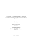
![An 8080 Simulator for the 6502, KIM-1 Version [1978]](http://vs1.manualzilla.com/store/data/005862327_1-86881d05118ae2e6f54412aa1d9ee60a-150x150.png)