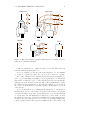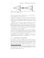
1
ÉCOLE POLYTECHNIQUE
PROMOTION X98
RAPPORT DE STAGE D’OPTION
SCIENTIFIQUE
The Geometry of Interaction and
Interaction Nets in Hardware1
Blaise
GASSEND
([email protected])
Option : Informatique
Département d’Informatique.
1 Version
du 17 janvier 2003.
Résumé
La géométrie de l’interaction et les réseaux d’interaction sont deux systèmes
permettant de décrire le calcul, et avec lesquels on essaye de faire des évaluateurs
logiciels performants. Au cours de mon stage j’ai étudié la possibilité d’utiliser
ces idées pour faire un évaluateur en hardware, afin profiter au maximum des
possibilités de parallélisme qui existent en éléctronique. Mes recherches m’ont
conduit successivement dans trois directions assez différentes. J’ai d’abord essayé de compiler le λ-calcul linéaire (qui utilise chaque variable exactement
une fois) en utilisant des systèmes à base de jetons, inspirés de la géométrie de
l’interaction. Puis, je me suis concentré sur un type de réseau d’interaction particulier, les combinateurs de l’interaction, qui est universel, et avec lequel j’ai cette
fois essayé de compiler le λ-calcul classique, toujours en utilisant ses systèmes
de jetons. Enfin, j’ai pris une approche assez différente des deux précédentes
pour essayer de développer un évaluateur de réseaux d’interaction qui utilise
la réduction de graphe. Un premier prototype permet de compiler le λ-calcul
linéaire, et j’ai de nombreux éléments qui devraient permettre d’étendre ce prototype à un évaluateur plus universel.
Abstract
The geometry of interaction and interaction nets are two systems with which
computation can be described, and that hold promise for designing high speed
software evaluators. During my internship, I studied the possibility of applying
these ideas to a hardware evaluator, to benifit from the inherint parallelism of
electronics. My research successively followed three fairly different directions.
First, I tried to compile the linear λ-calculus (which uses each variable exactly
once) with a token passing method inspired from the geometry of interaction.
Then I looked at the interaction nets formed by using the interaction combinators, a universal interaction system, with which I tried to compile the classical
λ-calculus, again with a token based method. Finally, I tried an approach that
is quite different from the two others, to try to develop an interaction net evaluator that uses graph reduction. A prototype was designed that can handle the
linear λ-calculus, and I have many ideas that should allow this prototype to be
extended to more general systems.
Contents
1 Introduction
1.1 Goals . . . . . . . . . . . . . .
1.2 Modeling a Circuit . . . . . . .
1.3 The Languages that were used
1.4 A brief tour of this Document .
1.5 Acknowledgments . . . . . . . .
2 The
2.1
2.2
2.3
2.4
2.5
2.6
2.7
2.8
.
.
.
.
.
.
.
.
.
.
.
.
.
.
.
.
.
.
.
.
.
.
.
.
.
.
.
.
.
.
.
.
.
.
.
.
.
.
.
.
.
.
.
.
.
.
.
.
.
.
.
.
.
.
.
.
.
.
.
.
.
.
.
.
.
.
.
.
.
.
Linear Case
The Linear λ-calculus . . . . . . . . . . . . . . . . . . .
Encoding the Linear λ-calculus with Linear Logic . . . .
The Geometry of Interaction Interpretation . . . . . . .
Possibility of Parallel Evaluation . . . . . . . . . . . . .
Handling Values of Base Type . . . . . . . . . . . . . . .
Information at Token Approaches . . . . . . . . . . . . .
2.6.1 Mastering the Amount of Information by Typing
2.6.2 Parallel Encoding . . . . . . . . . . . . . . . . . .
2.6.3 Serial Encoding . . . . . . . . . . . . . . . . . . .
2.6.4 One-Hot Encoding . . . . . . . . . . . . . . . . .
2.6.5 Casting from one Encoding to Another . . . . . .
2.6.6 Limits of the Information at Token Approach . .
Other Token Approaches . . . . . . . . . . . . . . . . . .
Adding Erasing . . . . . . . . . . . . . . . . . . . . . . .
3 Interaction Combinators
3.1 Interaction Nets . . . . . . . . . . . . . . . . .
3.2 The Interaction Combinators . . . . . . . . . .
3.3 The Geometry of Interaction Interpretation . .
3.4 Encoding the Full λ-calculus . . . . . . . . . .
3.5 Simplified graphical representation . . . . . . .
3.6 Adding the constants . . . . . . . . . . . . . . .
3.7 What I Worked on . . . . . . . . . . . . . . . .
3.7.1 Direct Stack Based Implementation . .
3.7.2 A Trivial Optimization of the Encoding
3.7.3 Typing Interaction Combinators . . . .
3.7.4 Understanding the Stacks . . . . . . . .
1
.
.
.
.
.
.
.
.
.
.
.
.
.
.
.
.
.
.
.
.
.
.
.
.
.
.
.
.
.
.
.
.
.
.
.
.
.
.
.
.
.
.
.
.
.
.
.
.
.
.
.
.
.
.
.
.
.
.
.
.
.
.
.
.
.
.
.
.
.
.
.
.
.
.
.
.
.
.
.
.
.
.
.
.
.
.
.
.
.
.
.
.
.
.
.
.
.
.
.
.
.
.
.
.
.
.
.
.
.
.
.
.
.
.
.
.
.
.
.
.
.
.
.
.
.
.
.
.
.
.
.
.
.
.
.
.
.
.
.
.
.
.
.
.
.
.
.
.
.
.
.
.
.
.
.
.
.
.
.
.
.
.
.
.
.
.
.
.
.
.
.
.
.
.
.
.
.
.
.
.
3
3
4
4
5
5
.
.
.
.
.
.
.
.
.
.
.
.
.
.
7
7
7
10
12
13
14
14
15
16
16
17
17
18
19
.
.
.
.
.
.
.
.
.
.
.
21
21
22
23
24
26
27
27
29
29
30
31
2
4 The Interaction Processor
4.1 The Concept . . . . . . . . . . . . . .
4.2 The Gamma Processor . . . . . . . . .
4.2.1 Message-passing Infrastructure
4.2.2 The naive γ agent . . . . . . .
4.2.3 A correct γ agent . . . . . . . .
4.2.4 Integers and Adders . . . . . .
4.3 Interconnection Network Architecture
4.3.1 Serial versus Parallel . . . . . .
4.3.2 Network Topology . . . . . . .
4.4 Arbitrary Interaction Nets . . . . . . .
4.4.1 Allocation . . . . . . . . . . . .
4.4.2 Interaction . . . . . . . . . . .
4.4.3 Erasing . . . . . . . . . . . . .
4.4.4 Reconfigurable Agents . . . . .
CONTENTS
.
.
.
.
.
.
.
.
.
.
.
.
.
.
.
.
.
.
.
.
.
.
.
.
.
.
.
.
.
.
.
.
.
.
.
.
.
.
.
.
.
.
.
.
.
.
.
.
.
.
.
.
.
.
.
.
.
.
.
.
.
.
.
.
.
.
.
.
.
.
.
.
.
.
.
.
.
.
.
.
.
.
.
.
.
.
.
.
.
.
.
.
.
.
.
.
.
.
.
.
.
.
.
.
.
.
.
.
.
.
.
.
.
.
.
.
.
.
.
.
.
.
.
.
.
.
.
.
.
.
.
.
.
.
.
.
.
.
.
.
.
.
.
.
.
.
.
.
.
.
.
.
.
.
.
.
.
.
.
.
.
.
.
.
.
.
.
.
.
.
.
.
.
.
.
.
.
.
.
.
.
.
.
.
.
.
.
.
.
.
.
.
.
.
.
.
.
.
.
.
.
.
.
.
.
.
.
.
.
.
37
37
39
39
39
41
43
43
43
45
46
46
48
48
50
5 Conclusion
51
5.1 My Contribution . . . . . . . . . . . . . . . . . . . . . . . . . . . 51
5.2 Gained Experience . . . . . . . . . . . . . . . . . . . . . . . . . . 51
A Software User Manual
A.1 Entering a λ-term . . . . . . . . . . . . . . . . . . . . . . .
A.2 Executing Commands . . . . . . . . . . . . . . . . . . . . .
A.3 Compiling the Esterel code . . . . . . . . . . . . . . . . . .
A.3.1 Compiling a Linear λ-term . . . . . . . . . . . . . .
A.3.2 Compiling into Typed Interaction Combinators . . .
A.3.3 Compiling into Two-Stack Interaction Combinators .
B Overview of the Source Code
.
.
.
.
.
.
.
.
.
.
.
.
.
.
.
.
.
.
53
53
54
55
55
56
56
59
C Interaction Combinator Graphical Interface
61
C.1 Outline . . . . . . . . . . . . . . . . . . . . . . . . . . . . . . . . 61
C.2 Setting Hooks . . . . . . . . . . . . . . . . . . . . . . . . . . . . . 62
Chapter 1
Introduction
1.1
Goals
The geometry of interaction and interaction nets are two ways of describing
computation, which have been developed throughout the 90s. Both systems
have given rise to experimental software evaluators that try to do efficient computation. The aim of my internship was to look at ways to put these ideas
into hardware, where the inherent parallelism could lead to further speed improvements. Most of my effort went into trying to find ways to encode various
fragments of the λ-calculus, though some of my efforts can also be used on
interaction nets.
From the beginning, I selected a number of criteria that give a better idea
of what I was looking for, and that helped guide my work :
Evaluation time : The main goal is to evaluate terms as fast as possible, so
the evaluation time of the completed circuit is a key factor.
Parallelism : The main hope in moving from software evaluation to hardware
evaluation is that a degree of parallelism will become possible. Though
this goal is very difficult, it is interesting to keep in mind as some strategies
are better suited to being parallelized than others.
Locality : To be satisfying, an encoding of a lambda term into hardware should
preserve the structure of the term. In particular, it would be desirable to
have a direct correspondence between each sub-term and an area of the
compiled circuit, as well as to be able to combine independently compiled
sub-terms into larger terms.
Polymorphism : Much of the power of the λ-calculus comes from its polymorphism, which allows one simple term to capture an algorithm that can be
applied on a whole range of types. An encoding in which polymorphism
would be preserved would be very satisfying. Imagine being able to simply
plug two terms together, without worrying what types they were compiled
for, to get a circuit for the application of one term to the other.
Circuit size : Circuit size is of course a limiting factor from the physical point
of view. However, it also impacts on compilation time since there are
3
4
CHAPTER 1. INTRODUCTION
optimization and placement steps that must be done before the circuit is
made, which have a cost related to circuit size.
Compilation time : Since the long term goal is to be able to quickly evaluate
a lambda term in hardware, it would be nice to keep the cost of compiling
lower than the cost of directly evaluating the expression. A slow compiler
can nevertheless be useful if the lambda term that is compiled can be
evaluated with various parameters.
Though meeting all, and even some of these objectives has proven to be very
difficult, they have been a great aid to evaluate the potential of a compilation
strategy.
1.2
Modeling a Circuit
In order to think about compiling into hardware, it is necessary to have an idea
of what is possible and what is not, what is too big, and what fits, what is too
slow, and what can be done in a reasonable time. To be able to evaluate all this
it is necessary to chose a model with which to work.
I chose to work in the synchronous logic model. It is the most widely used
model today, and there are proven methods for producing circuits in it. There
are also a number of languages to describe and simulate synchronous circuits.
Moreover, in choosing this model I remain sufficiently far from the technical
details of the fabrication process, which are irrelevant at such an early stage.
In choosing a synchronous model, I reduce the need for complex handshaking mechanisms without any major restrictions to what I can do. Moreover,
the advantages that can come from using an asynchronous model should be
applicable to the results I obtain here.
In restricting myself to logic circuits, I am simply clearly defining the amount
of information that can flow through one wire, and avoiding having to think
about factors such as noise that limit the amount of information in analog
machines. In any case, whatever can be computed with an analog machine can
be computed just as well with a digital machine as long as one is willing to use
more wires.
1.3
The Languages that were used
In order to describe synchronous circuits, a large number of languages are available. After a survey of existing free software, I was left hesitating between
VHDL, Verilog and Esterel. The first two are industry standards, VHDL being
of a more European flavor. A number of free tools exist for them, but none
seem to be equipped with all the features yet. Esterel is mostly used for circuit
verification, but is shipped with an easily usable and expandable simulator. It
has also been around for quite a while and is well established.
For my project, I finally opted for Esterel, because of its ease of use. All the
circuits that I generated were described using this language. I later found that
Lustre might have been a slightly better choice than Esterel because of a more
convenient type system.
1.4. A BRIEF TOUR OF THIS DOCUMENT
5
The other language that I used extensively was Objective Caml. I wrote
a number of circuit generation variants, all built around a common λ-calculus
parser.
1.4
A brief tour of this Document
Since the topic I had to study was quite vast, I approached it from a number
of directions during my three-month internship. In the sequel, I will cover the
three main approaches, each of which occupied roughly equivalent amounts of
time.
For the first few weeks, I tried to compile a simplified λ-calculus by using
token passing methods. Chapter 2 covers this simplified case. During this
period, I learned the basics of the geometry of interaction and of interaction
nets. When I read [MP01], which describes how to encode the full λ-calculus
using the very simple interaction combinators, I decided to try its approach in
hardware. The details can be found in chapter 3. Finally, in chapter 4, I present
what I think is my most promising work, a processor for interaction nets, which
uses graph reduction to carry out evaluation.
1.5
Acknowledgments
I would like to warmly thank Ian Mackie for offering me this internship at such
short notice, spending hours in his office discussing ideas with me, his positive
and encouraging attitude, and help in trying to weed this report of all the errors
that I put into it. It has been a pleasure having him as a supervisor. I would
also like to thank all the people whom I met at LIX for the pleasant atmosphere
around the lab.
Chapter 2
The Linear Case
2.1
The Linear λ-calculus
In what follows, I will often be making reference to the linear λ-calculus. I will
not be referring to the full linear λ-calculus that comes from full linear logic
through the Curry-Howard isomorphism, but rather to a simplified version that
comes from the exponential-free multiplicative fragment of linear logic, or from
classical logic without weakening or contraction rules.
The terms of the linear λ-calculus are in fact terms from the classical λcalculus in which each variable is used exactly once.
An example of a linear term is :
(λxy.yx)(λx.x)
The following well known terms are not linear because they do not use a
variable (2.1) or because they use one twice (2.2).
λxy.y
(2.1)
λxy.x(xy)
(2.2)
The linear lambda calculus is not very interesting as a programming language
because it is impossible to create or erase information in it, and consequently
it can only express trivialities. Nevertheless, it is a good starting point because
it is contained in the classical λ-calculus, and is in itself quite hard to compile
into hardware in a satisfactory way.
2.2
Encoding the Linear λ-calculus with Linear
Logic
There is a strong link between computation and logic. Indeed, the CurryHoward isomorphism applied to classical logic shows that a lambda expression
and a logical proof share a common mathematical structure. According to this
isomorphism, doing cut elimination on a proof is identical to doing β-reduction
on a lambda expression.
7
8
CHAPTER 2. THE LINEAR CASE
The Curry-Howard isomorphism relates in the same way the linear λ-calculus
and the multiplicative fragment of linear logic (made up with ⊗ and
connectives). I will not go into the details of the isomorphism or of linear logic,
which are not in the scope of my project. The curious reader can refer to
[Gir87, Gir95, Abr93] for more information. I will just give an example of how
to translate a λ-expression into a linear logic proof.
Formula 2.3 shows the translation of (λx.λy.xy) into a linear logic proof. The
actual formulas that appear in the proof are not a part of the proof itself. We
could use the same proof to prove other formulas by replacing a or b by arbitrary
formulas. In fact, in the Curry-Howard isomorphism, the formulas of the proof
representation are linked with the types of the λ-calculus representation. If we
write the conclusion (a ⊗ b⊥ ) a⊥ b of this proof using the linear implication
connective1 , we get ((a −◦ b) −◦ a) −◦ b, which nicely matches the type (a → b) →
a → b of the translated lambda term.
a⊥
axiom
a
a⊥
axiom
axiom
a ⊗ b ⊥ a⊥ b
b⊥ b
tensor
a ⊗ b ⊥ a⊥ b a ⊗ b ⊥ b
cut
a ⊗ b⊥ a⊥ b par
(a ⊗ b⊥ ) a⊥ b
par
((a ⊗ b⊥ ) a⊥ ) b
(2.3)
The proof notation is unfortunately weighed down by a lot of syntax. In
the case of the multiplicative fragment of linear logic, a proof can be described,
as is shown in [Gir87, Laf95], by a graph representation that does away with a
lot of the superfluous information. These graphs are called proof nets. Figure
2.1 shows the previous example as a proof net, as well as normal graph representation of a linear λ-term. To convert between the two representations, all
that needs to be done is to connect variables to their abstractions, and do the
substitutions shown in figure 2.2.
In the sequel, when describing net representations, I will refer to the left,
agents, when describing proof nets.
right and principal ports of the ⊗ and
The meanings of these words are self-explanatory.
In the graph net representation, computation is done by doing cut elimination steps. There are two cut elimination rules in the multiplicative fragment
of linear logic. The first eliminates an axiom with a corresponding cut :
..
..
A A⊥
A
..
..
axiom
A
cut
..
..
A
..
..
(2.4)
The second one moves a cut up one step in the proof through a ⊗ and
..
..
A
A
..
..
B
B
1 Using
..
..
..
..
⊥
A
B⊥
⊥
A ⊗ B⊥
a −◦ b = a⊥
..
..
A⊥
..
..
A
cut
b, (a ⊗ b)⊥ = a⊥
cut
..
..
B
..
..
B⊥
.
cut
(2.5)
b⊥ and (a
b)⊥ = a⊥ ⊗ b⊥
2.2. ENCODING THE LINEAR λ-CALCULUS WITH LINEAR LOGIC
9
y
x
@
y
&
λ
x
&
λ
Figure 2.1: The graph on the left is the proof net for (λx.λy.xy). Axioms and
cuts have been represented by thicker lines, but this distinction isn’t usually
made since an axiom can be recognized by its u shape, and a cut by its t
shape. Its structure reflects the structure of 2.3 but we no longer need to bother
with the formulas. The graph on the right is an upside-down version of the
standard graph representation of the λ-term. Dotted lines have been added
between matching variables to show the likeness of the two graphs.
x
y
@
x
x
λ
xy
&
xy
xy
Figure 2.2: The two rules to convert an upside-down graph representation of a
lambda term into a proof net.
10
CHAPTER 2. THE LINEAR CASE
&
Figure 2.3: Cut elimination in proof nets is very visual thanks to the electrical
analogy. It happens by eliminating zig-zags in the wires, and getting rid of
unnecessary multiplexer-demultiplexer pairs.
Cut elimination in the proof net representation happens very naturally using
Girard’s electrical analogy 2 . Connections between connectives, cuts and axioms
are all seen as wires. If two wires are plugged into each other they behave just
like a single wire. In this way the cut elimination rule in 2.4 can just be seen as
straightening a wire. The second rule also has an interesting electrical interpretation. If we consider
and ⊗ to be a sort of multiplexer and demultiplexer,
then a direct connection between a multiplexer and a demultiplexer can be reduced to a direct connection between corresponding wires. This is exactly what
happens in 2.5. Figure 2.3 shows the two rules for proof nets.
If we consider two proof nets to be identical if they differ only by application
of 2.4, then we find that rule 2.5 applied to a proof net has exactly the same
result as β-reduction applied to the corresponding lambda term. Figure 2.4
shows the correspondence.
Now that we have seen how a λ-term can be transformed into a proof net,
and how reduction of the λ-term is the same as cut-elimination on the proof net,
we will be able to apply proof net methods to do computation. The next section
will introduce the geometry of interaction that allows us to evaluate proof-nets.
2.3
The Geometry of Interaction Interpretation
The geometry of interaction is a way to assign a meaning to a net by assigning
weights to its edges, which was originally developed to give a semantics of linear
logic. More information can be obtained from [Gir89].
The values of the weights belong to an algebra that depends on the meaning
that we wish to give to parts of the graph. The weight of a path is the product
of the weights of its edges (the last edge in the path is at the leftmost position
in the product). A weight can be calculated between two nodes by adding the
weights of all the paths that go from one node to the other.
The graph that is considered by the geometry of interaction isn’t exactly the
net that we have seen above, but rather an unfolded version, in which a node is
split in two parts, one for tokens going up and one for tokens going down. The
edges of the graph are also appropriately split into two directed edges, one going
up, and one going down. Axioms and cut links make it possible to go back and
forth between the up and down directions. Another way of obtaining the same
result is to keep the original nets, but to disregard paths that turn around in a
connective.
2 See
[Gir95].
11
2.3. THE GEOMETRY OF INTERACTION INTERPRETATION
x
x
A
A
x
x
B
λ
B
B
A
@
A’
A’
B’
B’
B’
&
A’
Figure 2.4: Comparison between beta reduction (top row) and cut-elimination
(bottom row).
12
CHAPTER 2. THE LINEAR CASE
&
p
q
q*
p*
q* q
q* p
p* q
p* p
1
0
0
1
Figure 2.5: The two nets above are equivalent according to rule 2.5. For the
geometry of interaction to give them identical meanings, the weights of the four
possible paths from left to right must have the same weights in both cases.
Equations 2.6 come directly from equating the weights of corresponding paths.
In the cases that we will be considering3 , if we start building a path from
the root of the net, there is, at any given node, only one direction in which to
extend the path to have a non-zero weight. This means that evaluation using
the geometry of interaction can be done by moving a token around the net,
keeping track of the weight that it is carrying.
For the multiplicative fragment of linear logic, the algebra that is used is
particularly simple, as it is generated by two elements p and q. The path that
goes from the right (resp. left) side of a ⊗ or connective to the principal port
has the weight p (resp. q). The paths going in the opposite direction have the
inverse weights : p∗ (resp. q ∗ ) to go from the principal port to the right (resp.
left) port.
Figure 2.5 shows how the ⊗ − rule defines some key identities4 , which are :
p∗ p = 1, q ∗ q = 1, p∗ q = 0, q ∗ p = 0
(2.6)
For the paths that we will be considering, and after reduction by 2.6, the
weight will always be written as a product of ps and qs. It will never be necessary
to use p∗ and q ∗ . Thus a stack is an appropriate model for the algebra. Leftmultiplying by p or q is like pushing a value onto the stack. When entering the
principal port of a ⊗ or agent, the value on the top of the stack (on the left
of the product) will cancel out with the weight of one of the paths, and will be
zero with the other path, so we will pop the top element off the stack, and go
in the direction that doesn’t leave us with a zero weight. Figure 2.6 illustrates
how this works.
2.4
Possibility of Parallel Evaluation
.
3 Nets built from a lambda expression returning a value of base type. If the returned value
is not of base type, as is the case for a function, there are a number of non zero-weighted
paths that correspond to the different parts of evaluating the function.
4 These identities arise from our desire to have the same weight for two wires as for a
configuration where ⊗ and
are connected by their principal ports.
13
2.5. HANDLING VALUES OF BASE TYPE
pq...
q*ppq... = 0
1
3’
ppq...
2
&
p
q
q*
p*
3
p*ppq... = pq...
Figure 2.6: A token arrives at (1) with pq . . . at the top of its stack. It goes
through the connective, gaining a p on the top of its stack, and ending up at
(2). The token can then in principle move to (3) or (3’). However, if it moves to
(3’) then it ends up with a zero weight. Only by going to (3) will the token have
a non-zero weight. The weight of the token that exits in (3) is pq . . . just as it
was initially. Everything happened as if p was pushed onto the stack between
(1) and (2) and then popped off in (2) to choose between (3) and (3’).
In the various encodings that I have studied in this chapter, I have considered
that tokens leave from extremities (the root of the term, or a constant). This
excludes the possibility of evaluating bits of path and then multiplying the
results together to get the weight of the full path. In order to achieve that type
of parallelism, it would be necessary for two arbitrary connectives to be able
to communicate directly. In chapter 4 I will study a method that allows such
communication.
For now the potential source of parallelism comes from constant binary operators, such as addition. My hope in this chapter was to find an encoding that
would allow many tokens to flow through the circuit at once. At the beginning
there would be a single token, at the root of the term. When this token would
meet an adder (for example) it would split into two tokens. At some point these
tokens would return to the adder carrying an integer. After the rendez-vous,
one token would emerge with the result of the addition and would flow back to
the top of the term.
In an optimized version of the above, tokens would start at all the constants
and would flow around the term, coalescing at adders (for example) until only
one token would be left to reach the top of the term. This simplification works
because the paths of base type in the geometry of interaction are symmetrical,
starting at the root, going all the way down to the constants, and then following
the reverse path back up to the root.
2.5
Handling Values of Base Type
Up to now, we have only discussed compiling pure lambda expressions. In
practice, it will usually be desirable to have constants for integers, booleans, and
basic operators such as incrementation, decrementation, and the conditional5 .
A constant value (integer or boolean) will be inserted in the logic net as
5 The conditional takes one boolean parameter that allows it to select one of its two other
parameters. For the linear lambda calculus I chose to have a conditional operator that could
only handle values of base type (integers or booleans) otherwise it would have been necessary
to use parts of the additive fragment of linear logic.
14
CHAPTER 2. THE LINEAR CASE
an agent with one port. For the geometry of interaction, a token entering that
port will immediately exit by the same port, the weight associated with this
maneuver is a constant-specific element of the algebra.
A constant function will be added to the net as an agent with one output
port and a number of input ports. For a unary operator, a token incoming
on the output leaves by the input unchanged (multiplied by a unity weight).
When it later arrives at the input, it leaves by the output with for weight an
element of the algebra that operates like the function on the algebra element
that represents a constant value.
When we look at typing information, we see that there is no need for the
algebra element that represents a constant value to commute with p and q.
Indeed, when a constant value, or a function that produces a constant value is
reached, in a net constructed from a λ-term of base type, the product of the
traversed weights will always be unity. Because of this, only one constant value
will be carried at a time, so the algebra can be modeled as before by a stack,
except that a register has to be added to store the current base value if there is
one.
2.6
Information at Token Approaches
The geometry of interaction interpretation strongly suggests the possibility of
an electronic implementation of linear lambda expression evaluation. In this implementation each connective of the expression we wish to compile corresponds
to a physical location in the electronic circuit. A token is able to flow between
connected connectives, carried by one or many wires, following the rules of the
geometry of interaction.
The major problem with this approach is that the information that is carried
by the token is an element of the algebra, which is infinite. In a software
implementation, large amounts of memory can be allocated on the heap to store
the required information. Electronically, it would of course also be possible to
have a heap that the token could access. However, this would make it impossible
to have many tokens flowing around the term in parallel since they would have
to take turns accessing the heap. It is therefore desirable for a token to be able
to carry all the information it needs along with it.
2.6.1
Mastering the Amount of Information by Typing
Luckily, in the case of the linear λ-calculus, it is possible to know at compiletime how much information the token is going to be carrying around with it at
a given point in the circuit, if the type of the term is known6 . We will find that
the amount of information is closely related to the type of the term that has its
root at the current point in the circuit.
The type of the term can be seen as a binary tree, with a node for each →7 ,
and a leaf for each base type. Here are some properties of interest :
1. When the token arrives at a point in the circuit, if we start at the root
6 For
a term of polymorphic type, it is necessary to specialize the type variables.
rather for each −◦ since the function is linear, but I will dispense with this detail in
notation since there is no ambiguity.
7 Or
2.6. INFORMATION AT TOKEN APPROACHES
Register
Register
Multiplexer
Multiplexer
15
Figure 2.7: A parallel connective.
of the type tree, and descend into the tree using the values on the stack
(going left for a p and right for a q) we will exactly end up at a leaf.
2. Moreover, if we annotate the base types at the leaves of the tree with +
and - to show whether they are results or parameters8 respectively, we will
find that tokens going up (away from the root of the term) carry a constant
value only on parameter leaves, while tokens going down (towards the root
of the term) only carry one on result leaves.
3. Finally, for linear λ-terms without strange functions such as the conditional, each leaf of the type tree will be traversed exactly twice, once in
each direction.
The above properties can be proven by structural induction on the λ-term.
The consequences are quite valuable for us since they allow us to know
exactly how much information can flow through each point in the circuit. This
will enable a number of encodings that we will now study.
2.6.2
Parallel Encoding
In the parallel encoding a token is carried at a given point of the circuit by
the number of wires needed to carry the deepest stack that the token can be
faced with, as well as a wire to indicate the token’s presence and wires to carry
the current constant value. Connectives can then be simply implemented with a
multiplexer and a demultiplexer and some registers as in figure 2.7. The registers
are necessary because the token is likely to flow through the same connective
many times, though careful optimization could make some registers redundant.
A variant of the parallel encoding can be obtained by numbering the states
that the token can be in at a given point in the circuit. The token can then
be represented by the minimum number of wires that is needed to encode the
8 In a type such as a → (b → c), a and b are clearly parameters, while c is a result. To
generalize this intuitive idea, simply count the number of times you go left in the type tree.
Results have turned left an even number of times, while parameters have turned left an odd
number of times. If one were to replace A → B with A ∨ B, then one would find that types
that after application of DeMorgan’s laws, types that are not complemented are results, while
complemented types are parameters.
16
CHAPTER 2. THE LINEAR CASE
number of states. In general this approach will use fewer wires, but this advantage will be completely over-balanced by the increase in complexity of the
connectives.
2.6.3
Serial Encoding
This encoding tries to reduce the size of the circuit compared with the parallel
encoding. Instead of sending the token’s information in parallel, we now send
in a bit-serial manner, with the top of stack first. In this way the first bit of the
token that arrives is able to direct the token in the right direction when there
are two paths to choose from.
With this approach it is necessary to add delays on some of the links to
ensure that the first bit of the token will never run into the body of the token
as it loops around the graph of the term. These delays mean that the serial
encoding will be slower than the parallel encoding.
The length of the delays that have to be added on links depend on the typing
information, and therefore on the global structure of the term. I tried a number
of methods to get rid of the delays, in order to make a serial encoding that can
be built locally from the proof net of the term.
Some of my most promising attempts involved misrouting a blocked token
towards the tail of the impeding token, in order to keep the information flowing,
and to avoid deadlock. Unfortunately I was able to find single-token deadlock
scenarios for each scheme that I came up with.
2.6.4
One-Hot9 Encoding
This encoding is by far the simplest electronically. When considered on paper
it seems to produce huge circuits, but in fact the whole circuit simply reduces
to the various constants that appear in the term, connected by direct links.
The idea is that at a given point in the circuit there will be one wire for each
possible token state. Since a token will only go through a given link in a given
direction with a given state once during evaluation, it is no longer necessary
to delay the token at the connectives. Moreover since a token arriving at a
connective in a given state will always leave the connective in a predetermined
direction and state, the connectives will just be wirings between incoming wires
and outgoing wires.
The number of wires that interconnect connectives, can grow exponentially
with the size of the term that is being compiled. Consider for example :
(λx.x)(λx.x) . . . (λx.x)
The leftmost (λx.x) will be traversed a number of times that grows exponentially with the size of the term.
Fortunately, after simplification of the wires using the connections that are
made in the connectives (something that is always done before producing a
circuit on silicon), the number of wires in this example reduces to one.
If there are constants in the circuit the number of wires will be the number
of ports of the constants plus the size of the type of the full term. All the
9 The term one-hot is used when making finite state machines in which each state has its
own register.
17
2.6. INFORMATION AT TOKEN APPROACHES
structure of the lambda term will have disappeared, and only the operations
on base types will remain. In a way this is an optimal encoding of the linear
lambda term.
2.6.5
Casting from one Encoding to Another
The encodings that I have described are in fact not incompatible. It would be
perfectly possible to mix terms compiled with two different approaches by using
simple casting circuits.
Table 2.1 shows the central element in a converter from one encoding to
another.
From Parallel
From Serial
From One Shot
To Parallel
Nothing
Shift Register
Priority Encoder
To Serial
Shift Register
Nothing
Go Via Parallel
To One Shot
Demultiplexer
State machine
Nothing
Table 2.1: This table gives a rough idea of how to cast from one encoding to
another.
Most lambda expressions have free type variables in their type. At compile
time we have to specify these free variables in order to determine the maximum
stack depth in the circuit. Thus λx.x won’t compile the same way if it is typed
as int → int or as (int → int) → int → int. A more elegant possibility is to
compile λx.x with type unit → unit, which will give a circuit of minimum size.
The resulting circuit can the be interfaced to a circuit that needs a larger type
through a caster that stores the extra type information when the token enters
the term, and restores it when leaving the term.
2.6.6
Limits of the Information at Token Approach
Now that I have given three encodings of the linear lambda calculus into hardware, and shown how casting can allow arbitrary mixing between encodings, it
is time to return to the goals that I outlined in section 1.1, to see how well they
have been met.
Evaluation time : In the one-hot encoding, the circuit is reduced to the necessary operators, connected by wires. Things can’t get much better than
that. With the parallel encoding, there is an added cost that is related to
how much the information has to flow around the circuit between operators. In the serial encoding the cost is even greater as it increases with
the amount of information that has to be moved.
Parallelism : Since the token will only flow through a given point in the circuit
in a given state once, the one-hot encoding allows many tokens to be in
the circuit, as long as the constant functions can’t cause collisions10 . This
means that with a one-hot encoding, many calculations can be carried
10 The conditional can cause collisions, for instance if two tokens are leaving the then and
else branches simultaneously.
18
CHAPTER 2. THE LINEAR CASE
out in a pipelined way11 . Another possibility is to do one calculation at
a time, but have tokens split in two at binary operators, as described in
section 2.4. For the serial and parallel encodings only one token can be at
a point in the circuit at a time, so parallelism is out of the question. The
same thing is true if casting is used, since the cast logic can only store
the information for one token at a time, and thus only one token can be
present under the caster.
Locality : All the encodings have a direct correspondence between the topology of the circuit, and the topology of the graph of the lambda term. In
the one-hot encoding, however, since most of the circuit is just wiring,
optimization will tend to break the correspondence.
Polymorphism : None of the encodings are directly polymorphic, though they
all produce circuits that can be used on smaller types12 than they were
compiled for. With casting, terms can be used in a fully polymorphic way.
Circuit size : Unless we consider that large entities such as adders should only
appear once in the circuit, the one-hot encoding is as compact as can be
expected. The other two encodings are somewhat larger since they contain
logic that regulates the flow of the token around the circuit. The serial
encoding is smaller than the parallel encoding.
Compilation time : The three encodings rely heavily on typing information.
Since types of a sub-term can have a size that is exponential with the
size of the full term, compilation time can be exponential. This is unfortunate considering that the linear lambda calculus can be reduced in a
linear number of steps by simple graph reduction13 . Because of this these
encodings can only be useful if the resulting circuit is to be used many
times.
It is interesting to note that for a pure linear λ-term (without constants),
the most general type of the term directly leads to the one-hot encoding,
all one needs to do is connect corresponding type variables. This means
that in looking for the type, we have in fact evaluated the linear λ-term.
Globally, the various encodings are not very satisfying, even for something
as simple as the linear λ caluclus. This encouraged me to try other approaches.
2.7
Other Token Approaches
Since the major problem with the approaches seen so far is that the token has
to carry all its information around with it, I tried exploring other possibilities.
Some of these possibilities will be used in later chapters.
Information at Origin : With this type of approach, the stack elements are
left wherever they were created. The idea is that this will prevent the
11 This is interesting if the constant values can be changed for each successive token to do
the same calculation on many different imput values.
12 A smaller type is a type whose tree is included the tree of the larger type.
13 It should be noted that an encoding very close to one-hot can be obtained in linear time
by using graph reduction.
2.8. ADDING ERASING
19
token from carrying large amounts of information into small subterms
where they won’t be needed. By some mechanism, the token keeps track
of where the information is stored, in order to fetch it when necessary.
One promising approach was for each connective that is traversed by the
token to remember where the token came from. In this way if the token
needs to know which way to go it can simply ask behind it. Since the path
that leads back to the information can get very long and can go through
the same parts of the circuit many times, it is necessary to reduce loops
that appear in the remembered path, when they contain no information.
This method remains quite complicated, and there are always cases in
which it is necessary to remember a path that goes through the same part
of the circuit many times; It is not yet clear exactly what determines the
maximum number of tims.
Global Information : Storing the information at a global location eliminates
the need to carry anything around with the token. However all hope of
parallelism vanishes. This approach is used in chapter 3.
Interaction Based : Instead of using the geometry of interaction, we can try
to somehow do graph reduction directly. This is what is developed in
chapter 4.
2.8
Adding Erasing
In this chapter we have entirely dealt with the linear λ-calculus where each
variable is used exactly once. It is in fact possible to extend all the results of
this chapter to the linear λ-calculus with erasing, in which variables are used at
most once. Indeed, unused variables will just correspond to parts of the circuit
that are never reached by a token.
If there was some sort of parallelism in the circuit, that came, for instance,
from starting tokens at all the constants at the beginning of evaluation, the
situation would be more difficult. Indeed, tokens that are useless because they
end up in unused variables would uselessly move around the circuit slowing
down tokens that are useful.
Chapter 3
Interaction Combinators
3.1
Interaction Nets
Interaction nets were introduced by Lafont in [Laf95]. They generalize the proof
nets of chapter 2. Their strong confluence properties make them particularly
interesting to work with. Because of our knowledge of proof nets, I will give
as a foot-note the proof net element that corresponds to each element of an
interaction net.
The first ingredient we need is a set of agents 1 . Each agent has one principal
port and zero or more auxiliary ports 2 . An interaction net is made up of agents,
some of whose ports have been connected by wires3 . There can be free ports
that are not connected to another port. There can also be wires that are not
connected to any agent. They provide the net with two extra free ports each.
Loops of wire are also a possibility, they of course provide no free port. The
interface of an interaction net is made up all its free ports.
The above definition of an interaction net is completely static. We still do
not know how to compute. Computation is done by adding a set of rules, so
that we get an interaction system. A rule transforms a net made up of two
agents and a wire connecting their principal ports into another net that has the
same interface4 . Agents connected by their principal ports make up an active
pair. There can only be one rule per pair of agents, and rules that apply to
a pair of identical agents must be symmetrical. In this way there is at most
one rule that can be applied to an active pair, and exactly one way to apply
it. Reduction of an interaction net proceeds by applying any rule that can be
applied until no active pairs remain. Since agents only have one principal port
each, and since rules always operate on active pairs, there can be no interference
between simultaneously applicable rules. Therefore the order of application of
rules is of no importance. This gives a rough idea of where strong confluence
comes from. For the details, refer to [Laf95].
1⊗
and
in proof nets
⊗ and , the inferred port is the principal port, the other two ports are auxiliary
2 For
ports.
3 Just as the wires of proof nets connect agents. There is no longer any need for axioms or
cuts.
4 The ⊗cut-elimination step replaces two agents connected by their principal ports into
two wires. The number of auxiliary ports before and after is four.
21
22
CHAPTER 3. INTERACTION COMBINATORS
ε
δ
ε
ε
ε
ε
ε
γ
ε
δ
ε
γ
γ
γ
δ
δ
γ
δ
γ
δ
Nothing
Figure 3.1: The interaction combinators reduce according to six very simple
rules.
In the rest of this chapter, we will be using one particular interaction system,
that will be introduced in the next section. In chapter 4 we will explore a way
that could with time lead to hardware evaluation of arbitrary interaction nets.
3.2
The Interaction Combinators
In [Laf97], Yves Lafont describes an extremely simple interaction system with
three types of agents : γ, δ and . He also proves that this system is universal
because any other interaction system can be translated5 into it. By analogy to
the S and K combinators that form a universal subset of the λ-calculus, Lafont
named his interaction system the interaction combinators.
Figure 3.1 shows the six reduction rules for the interaction combinators. The
γ − δ rule is particularly important for the universality of the system as it is the
only one in which agents are created.
The interaction combinators seem very interesting to me because they are
very simple locally, and yet remain universal. Since I am trying to compile each
agent as a separate entity on a chip, it is vital that each entity have a behavior
as simple as possible.
The γ and δ agents are almost identical, and can in fact be interchanged with
only slight modifications to the structure of the interaction net. The difference
is however necessary for translation of arbitrary interaction nets into interaction
combinators to be possible. Traditionally6 gamma and delta agents are given
very different functions.
A γ agent is used as a multiplexer, to group information in bundles. Its use
closely resembles the use of and ⊗ in chapter 2.
5 A translation is a transformation that replaces each agent of an interaction net by another
interaction net.
6 The use of γ and δ that was made in [Laf97] started this tradition.
23
3.3. THE GEOMETRY OF INTERACTION INTERPRETATION
γ
γ
γ
γ
γ
γ
γ
γ
γ
γ
Figure 3.2: With a tree of γ agents it is possible to multiplex together as many
wires as one desires. There are many ways to multiplex a given number of
wires together, but the only way to demultiplex them is with a second tree
that is symmetrical to the first one. This figure shows some trees that could
be used for abstraction and application in the encoding of the lambda calculus
into interaction combinators.
A δ agent is used to make copies of subnets made up of γ and agents. It
turns out that copies can be made of arbitrary nets by pulling the δ agents out
of the net before copying. The encoding of the λ-calculus will give an idea of
how this can be done.
In the sequel, it will often be useful to multiplex more than just two wires
together. This can be done easily with trees of γ agents (see figure 3.2). Care
has to be taken because in general the multiplexer is not identical to its corresponding demultiplexer. Instead the auxiliary ports of the γ agents have to be
permuted. Any tree of γ agents with the right number of ports can be chosen,
but balanced trees are likely to reduce faster in parallel implementations.
3.3
The Geometry of Interaction Interpretation
In the present chapter, I will be trying to compile interaction combinators into
hardware using geometry of interaction ideas, once again. In this case we have
an algebra that is just slightly more complicated than for the multiplicative
fragment of linear logic.
Indeed, we now have two types of multiplexers, one of which is twisted. We
will give each type of multiplexer two algebra elements that we will call : pγ ,
qγ , pδ , qδ . The δ rules will behave just like the ⊗ − rules :
p∗δ pδ = 1, qδ∗ qδ = 1, p∗δ qδ = 0, qδ∗ pδ = 0
For the gamma rules, the twist in the rule has disappeared which makes for
a slight change :
p∗γ pγ = 0, qγ∗ qγ = 0, p∗γ qγ = 1, qγ∗ pγ = 1
Since the γ − δ rule makes γ and δ agents move through each other without
interfering, γ subscripted elements commute with δ subscripted elements. Because of this commutation rule, when we have a product of algebra terms, we
can move the γ elements to the front of the product, and the δ elements to the
24
CHAPTER 3. INTERACTION COMBINATORS
Root door
Root door
...
Copy doors
δ
Variable doors
Figure 3.3: On the left is a net that is being built. It still has free variables, and
it has a port through which it makes copies. On the right is a net that has been
finalized by putting a copy operator (a δ agent) on its copy port. Note that the
finalized term has no variables. Indeed, the terms that would be plugged into
the free variable ports must be δ-free and there is no room left to connect the
variable’s copy port. It would be possible to leave room for each free variable
to have a copy port. For simplicity, and without loss of expressive power, I will
only consider finalized terms without any free variables.
back. This decomposes the algebra into two parts that can each be modeled by
a stack, as in the logic net case. All the details can be found in [Laf97].
In this way the geometry of interaction has shown us how to evaluate a net
of interaction combinators using a token that carries two stacks. The rest of
this chapter will try to put this into hardware.
3.4
Encoding the Full λ-calculus
To encode the λ-calculus with interaction combinators, I used an encoding from
[MP01]. The encoding I used is the so called call-by-value or !(A → B) encoding.
In chapter 2 the abstractions and applications of the linear λ-calculus were
represented by the ⊗ and of linear logic, acting as a multiplexer-demultiplexer
pair. Now we wish to move on to the full λ-calculus. For this we need to be
able to copy and to erase information. As was seen in section 2.8, erasing isn’t
a big problem. With the interaction combinators, we just have to add agents
on branches that we wish to erase.
Copying is a much trickier problem. δ agents can be used to copy nets that
are only made up of γ and agents. But this doesn’t tell us how to copy a
net that contains a δ. The trick to solving this problem, is to leave the copying
agent out of the net. This is done by adding copy ports to the interface of the
net. The net is built with the assumption that when it is used, a copy agent
will be connected to these ports. The net in itself can in this way be made up
entirely of γ and agents, and therefore be copyable, and still have the ability
to make copies. The encoding of the λ-calculus will make this much clearer.
Because of the copy-extraction that I have just described, compiling a lambda
term will be done in two steps. In the first step, a δ-free net will be generated.
It will have a principal door at the top, auxiliary doors at the bottom for free
variables, and copy door on the right hand side. Once the whole lambda term
is built, it can be finalized into a working interaction net, as in figure 3.3, by
adding a δ agent on the copy doors.
3.4. ENCODING THE FULL λ-CALCULUS
Abstraction
abstract
25
Application
ε
γ
ε
γ
ε
γ
γ
γ
γ
apply
Variable
Copy
Erase
ε
γ
ε
γ
ε
γ
ε
Figure 3.4: Encoding a lambda expression with interaction combinators is done
using a few elementary structures.
I will now explain how to compile each part of a λ-term. The reader can
follow the different steps in figure 3.4.
To encode a variable, we directly connect the principal door to the auxiliary
door. Since no copying is necessary, the copy doors are connected to agents.
The coding of abstraction is constrained by the fact that we would like to be
able to copy a term simply by making a copy of its principal door. This means
that we have to make the copy door of the unabstracted term come through the
principal port of the abstracted term. We will do this by multiplexing together
the abstracted term’s principal door, the abstracted variable’s door as well as
the copy doors. We then have to add epsilon agents to fill the unused copy doors
of the new net.
To encode an application, we demultiplex the principal door of the function.
As in the linear case, we connect what corresponds to the variable to the parameter term, and what corresponds to the the principal door becomes the principal
door of the new term. Unfortunately we now have two copies to make, one from
the parameter term, and one that was demultiplexed from the function term.
To make both copies with only one set of copy doors, we simply multiplex the
sources together as well as the respective destinations. We can now make both
26
CHAPTER 3. INTERACTION COMBINATORS
Root of the Term
Delta Agent
Abstraction Multiplexer
Three Epsilon Agents
Figure 3.5: The identity, λx.x, compiled into interaction combinators. We can
see an abstraction, a δ agent and two groups of three agents.
copies with just one set of copy doors7 .
The encoding described above is sufficient to encode a linear lambda term.
To encode any term we still have a little work to do. When encoding abstraction,
I implicitly considered that exactly one auxiliary door was being abstracted.
What if the variable that we are abstracting appears more than once, or not
at all? Variables appearing more than once can be merged together by using a
copier. If many copiers are necessary, they can be combined with multiplexers
in a similar way to the two copies that appear in an application. In the case of
unused variables, an agent can absorb the incoming variable.
3.5
Simplified graphical representation
After spending a lot of time hand-drawing compiled lambda terms, I decided
that an automated drawing tool would be useful. This section describes the
graphical conventions that were used by the one that I wrote, and that will be
used for the figures in the following sections8 .
I designed my drawing routines to draw agents very small in order to allow
easy visualization of large lambda expressions. The figures included here have all
been enlarged. Since patterns of γ agents such as abstraction, application and
sharing copy doors occur very often, they have been represented in a compact
manner. A few examples should get the reader familiar with the representation.
Figure 3.5 shows λx.x compiled into interaction combinators. The abstraction multiplexer is represented as a triangle pointing up. The variable and the
result enter through the bottom of the triangle, while the copies enter by the
right hand side. This is done to make the structure of the lambda term stand
out. Also note that for the same reason, the copy wires are lighter than the
main stream wires. The delta agent is a little triangle pointing right. It always
appears in exactly the same place so it doesn’t have to stand out. agents are
shown as a darker segment blocking off the end of a wire, in many cases they
are run together to save space.
In Figure 3.6 we have a slightly more complex term. There is an application,
a triangle pointing down, with the same disposition as the abstraction. There
are also a couple of triple γ agents, that are used to share copies. The three
gammas are represented as one triangle pointing south-west. Wires coming from
7 What we have done here is simply copy a pair instead of copying the sides of the pair
separately.
8 The figures with large pixels are computer-generated.
27
3.6. ADDING THE CONSTANTS
Root of the Term
Copy Multiplexers
Application Multiplexer
Figure 3.6: The identity applied to itself, (λx.x) (λx.x), compiled into interaction combinators. We can see an application, and some triple gamma agents
used to share the copy door of a term, as well as the agents that we had already
met up with.
the left are paired with wires coming from the bottom by a γ agent into wires
emerging from the right. The top, middle and bottom wires match with the
left, middle and right wires, respectively.
3.6
Adding the constants
Constants are added much as they are in the linear case, since the constants
can simply be seen as extra agents. Base values are an agent with no auxiliary
ports, and constant functions have one port per parameter and one for the result. Initially, a constant function has its principal port directed towards one
of its parameters. When the parameter arrives, the constant function is transformed so that it is ready to accept a new parameter. Lafont gives some specific
encodings in [Laf95], others encodings, which use infinite classes of agents, can
easily be developed, and are better suited to real life applications9 . The main
difference is that only the gamma stack is empty when a value of base type is
reached, as the delta stack must retain information about which of many paths
led to the value. This means that there is no need for rules of interaction between γ and a constant. Rules will however be necessary for encounters between
δ or agents and constants. These rules will simply copy or erase the agent as
in figure 3.7.
There is however an extra constant to be added, which is the fixed-point
combinator. The fixed point combinator can actually be encoded with γ and δ
agents. No specific agent is necessary. Figure 3.8 shows the encoding of the fixed
point combinator. We could actually do without the fixed point combinator
since it can be encoded directly in the full lambda calculus. However, such
encodings are very inefficient.
3.7
What I Worked on
As far as the interaction combinators are concerned, I tried out a variety of
ideas. None of them were particularly successful so I finally moved on to the
9 An integer, for example would be represented by zero instead of being represented by the
nth successor of 0
28
CHAPTER 3. INTERACTION COMBINATORS
? ...
? ...
δ
δ
...
? ...
δ
ε
ε
? ...
...
ε
Figure 3.7: A δ agent copies whatever it meets except another δ-agent. An agent erases whatever it meets.
Fixed−point
δ
δ
apply
function
Figure 3.8: On the left, is an encoding of the fixed-point combinator that shows
what we are trying to do : copy the result of an application and use it as a
parameter to the same application. On the right, is the same net with the
copy extracted, and with the function that is to be applied extracted, as it is
generated by my program.
3.7. WHAT I WORKED ON
29
interaction processor concept. Some of these results could be of interest to
others who might explore computation with interaction combinators.
3.7.1
Direct Stack Based Implementation
In order to observe term evaluation, and to try out some optimizations that
will be covered in the next section, I wrote some code to compile a λ expression
into Esterel using two global stacks. This implementation also used a global
register to store integer and boolean constants, and had only one incrementer
and decrementer that operated on them. Though it is quite slow, and impossible
to parallelize directly, this implementation shows a sequential encoding of a
geometry of interaction into hardware that could easily be generalized to most
geometry of interactions. It is the hardware equivalent of Mackie’s geometry of
interaction machine, from [Mac95].
The resulting circuit is in two barely connected parts. On one hand the data
part keeps track of the stacks, and the constant values. On the other hand, in
the sequencing part, a token flows through a circuit whose topology is very close
to that of the interaction net. As the token moves around the sequencing part,
orders are sent to the data part to push or pop a value, or to do an operation
on the value register. When it reaches a fork, the data part tells the sequencing
part which way to proceed.
In a geometry of interaction machine10 , there is a difference in the sequencing
part, since it is executing assembler code rather than having a token flow around.
The data part, however could be identical for both machines.
I find this resemblance quite inspiring though I do not really know what to
do with it.
3.7.2
A Trivial Optimization of the Encoding
Before producing an electronic circuit, it is profitable to do as much optimization
as possible. Let us look at two simple rules that can drastically reduce the
number of agents that are needed for a circuit.
One sub-expression that frequently turns up in expressions is (λx. . . .)(. . .).
In the λ-calculus terminology, this is called a redex. With interaction combinators, it is encoded as a multiplexer running straight into the corresponding
demultiplexer. It would be foolish to leave such a structure in an circuit, since
nothing is lost by doing the reduction at compile time11 . With a little generalization we find that much useless work can be avoided by doing all the γ − γ
reductions at compile time. This reduction phase terminates, just as in the
linear case, because each reduction reduces the number of agents by two.
In fact, further optimizations can be done by normalizing the net while
excluding γ − δ reduction, though in fact the γ − γ rule is the one that gives
the most improvement12 . With these reductions, we are getting rid of some
structure that was imposed by the λ-calculus, but that didn’t play an important
10 It
must not have been optimized to jump straight back after finding an answer
in the one-hot encoding of chapter 2 we were effectively doing all the multiplexer
reductions at compile time, which could at times give an exponential reduction in geometry
of interaction path length.
12 In fact, the δ − δ reduction will never be applicable.
11 Indeed,
30
CHAPTER 3. INTERACTION COMBINATORS
γ
δ
γ
δ
γ
δ
Figure 3.9: By exchanging γ and δ more reduction can be done at compile time,
leading to greatly optimized circuits.
part in the computation. We have rearranged the pipes to make them shorter,
but the appliances haven’t changed in any way.
Further optimizations can be obtained by doing some non-interaction-net
reductions. Two γ agents back to back can be reduced to a wire and two δ
agents back to back with a twist in the connection can likewise be reduced. We
can also replace a γ or δ agent with both auxiliary ports connected to agents
by an agent. These reductions are easily seen to be valid with the geometry
of interaction.
Still, it turns out that as terms are evaluated, much time is spent multiplexing wires together to go through the single delta operator, just to be demultiplexed again. The presence of the delta prevents the reductions that we
have discussed above. In fact, if we draw the interaction net as a set of trees
of agents with principal ports pointing down, we find that after the optimizations described above, we have exactly two trees. They are entirely made up
of gamma agents, except for one delta agent at the root of one of the trees,
preventing any interaction from happening13 .
It is clear that we cannot start using the γ − δ rule14 because it would cause
the net to grow, possibly without bound. There is, however, a change that
leaves the size of the net unmodified and that unblocks the situation. The idea
is to replace a δ agent with γ agents connected to its auxiliary ports by the
same configuration with γ and δ exchanged, as in figure 3.9.
After all the above reductions have been exhausted, we end up with an
interaction net where all active pairs are γ − δ pairs, and each δ has at least one
auxiliary port that is not connected to a γ principal port.
3.7.3
Typing Interaction Combinators
Since typing was so useful for compiling the linear λ-calculus, I spent some
time exploring type systems for the interaction combinators. Two type systems
I explored are shown in figures 3.10 and 3.11. I refer to them by γ and γδ
respectively. It is easy to make interaction nets that are untypable with both
of these systems by connecting a gamma agent’s principal port to one of its
auxiliary ports. Typing also fails on lambda terms. With the γδ type system,
13 Indeed, initially, there was only one δ agent, and no new δ agents were created by the
previous reductions. The only exception is for terms that don’t actually make copies, where
the δ agent gets removed by agents. Since the only reduction that hasn’t been done is γ − δ,
if there is anything left to do it will be such a reduction. And there can only be one active
pair since there is only one δ agent.
14 At least not as a simple optimization strategy
31
3.7. WHAT I WORKED ON
Basic Type Rules
A+
A+
Type Complementation Rule
A−
γ
<A−,B−>
B+
A+
A+
δ
A+
ε
A−
A+
A−
B+
B−
γ
B+
A+
<A−,B−>
<B+,A+>
γ
A−
B−
<A−,B−>− = <A+,B+>
Figure 3.10: A type system that is almost suited to λ-expressions compiled into
interaction combinators. A delta agent can only make copies of identical type.
On the left are the typing rules for the different agents. On the right is an extra
rule that is used to complement a type, and that is deduced from the γ − γ
interaction rule.
any recursive λ-term fails to type. With the γ system, describing which terms
is more subtle15 , I would not have found any without writing the compiler first.
A direction that I have good hopes for, but haven’t had time to explore, is to
use the γδ type system, allowing a few wires with typing errors. The whole term
can then be compiled with the one hot encoding, with re-entrant casters (which
will need two stacks, most likely) to handle the type mismatches. Perhaps more
imaginative type systems can actually make the casters become part of the type
system16 .
It is hard to say much more without writing more code and doing more tests,
as the types get very large very fast because of the copy doors.
3.7.4
Understanding the Stacks
To try to optimize the simple two stack implementation of the interaction combinators into hardware, I did some exploration of the operations that take place
on the stack during computation. To do this exploration I wrote a program to
generate a graphical representation of the term compiled into interaction combinators, and then to be able to step through execution while watching the token
15 I originally expected the γ type system to work for all typable λ-terms, and thought that
the typing errors I was getting were a bug because they appeared in strange ways. Then I
realized that since this type system allows compilation into a single stack finite automaton,
the terms that it types cannot be Turing complete.
The actual typing error occurs when the δ agent is added, so there should be a way to get
around it with a little work (including an extra stack). The error occurs when a function is
applied to a term that contains another copy of the same function. Indeed, in that case, the
type of the copy part of the function must be included in itself. So unless the function makes
no copies at all this situation will lead to an error.
16 A type system with a type A such that A = hA, Ai = hhA, Ai , Ai would allow situations
that cause type conflicts to enter the type system. It is not clear, however that the resulting
type system would have a natural encoding in hardware, as it would certainly require at least
two stacks to function.
32
CHAPTER 3. INTERACTION COMBINATORS
Type Complementation Rules
A+
A−
B+
B−
Basic Type Rules
A+
A+
A+
A−
γ
A+
B+
δ
ε
<B+,A+>
B+
<A−,B−>
B+
<A−,B−>
γ
A−
γ
B−
<A−,B−> = <A+,B+>−
A−|B−
A+
B−
B+
A−
A+
A+
A−|B−
δ
B+
A+|B+
δ
B−
A−
A−|B− = (A+|B+)−
Type Connective Inversion Rule
A−
A+
B+|A+
δ B−
C+
γ
<A−,C−>
D+|C+
δ C−
B+ γ
<B−,D−>
D−
B+|A+
D+|C+
γ
D+
<B−|A−,D−|C−>
<D+,B+>|<C+,A+>
δ
<A−,C−>
<B−,D−>
<D+,B+>|<C+,A+> = <B−|A−,D−|C−>− = <D+|C+,B+|A+>
Figure 3.11: A type system that treats γ and δ connectives as similarly as
possible. The top left quarter rules show how to type each agent. The top right
quarter derives type complementation rules from the γ − γ and δ − δ rules. The
bottom half derives a rule that allows the permutation of type connectives.
3.7. WHAT I WORKED ON
33
copy
agent
Figure 3.12: On the left, the lambda term λx.xx is represented, with its copy
agent explicitly shown. The bottom wire on the left hand side is the variable
that is being copied, and the wires above it are the copies. The three wires
at the top are the copy ports that the copy agent uses to actually make the
copies. Copy mode is entered (possibly recursively) when the token enters the
copy agent from the left, and is exited when the token exits to the left. On the
right, λx.xxxx is shown. This case is a little more complicated because three
binary copy agents are needed. The copy agents are represented by rectangles.
In two of the rectangles the source of the copy enters through the left of the
box. When a copy of the variable is made in this case, copy mode is entered
and exited twice.
flow through the net17 .
Two Modes of operation
The first noticeable fact is that there are two quite distinct modes during computation. In the first mode, that I will call normal mode, the gamma stack is
used in exactly the same way as the single stack of chapter 2. In particular the
copy ports of the abstraction and application agents are never used. In normal
mode the δ stack is never changed.
The second mode, that I will call copy mode, is entered whenever a variable
is used more than once. When the variable is used exactly twice, it is entered
on leaving the variable port of an abstraction and is exited just before the use of
the variable. Is is also entered and exited in the same places when the token is
traveling in the other direction. The transition corresponds to the grayed paths
in the graphical representation that my program generates. If we were to draw
the interaction net with copy agents drawn instead of uses of the copy door of
the term, copy mode would be effective between the moment when the token
enters the copy agent and the moment when it leaves it. This can be seen for
two or more copies of the variable in figure 3.12.
The goal when passing through copy mode is to add or remove a mark from
the δ stack. When going from the variable’s use to the variable port of the
abstraction, a mark is added to the δ stack to say which use of the variable the
token will have to return to. When going in the other direction, the mark is
17 Interaction
nets represented by this program have already been shown in section 3.5.
34
CHAPTER 3. INTERACTION COMBINATORS
removed, and the token exits copy mode at exactly the place where it entered.
When in copy mode, the token gets multiplexed a number of times, then
enters the delta agent, or a copy port of an abstraction. In the latter case, it
flows around the net and ends up leaving a copy port of an application agent,
at which point, it will once again be multiplexed before entering a delta or an
abstraction copy port. In the end the delta agent is always reached. During all
this, the gamma stack from before copy mode was entered is unaffected.
The path that the token follows to get to the delta is very important. Indeed,
the mark that is added or removed when passing through copy mode isn’t in
general placed on the top of the stack. This means that some marks have to
be removed before the mark that we are concerned with can be manipulated.
These marks then have to be replaced.
These marks that have to be removed then replaced are found when the token
goes between a copy port of an abstraction and a copy port of an application.
During this time, the token can go through a number of copy operations, as if
copy mode were entered recursively, it is with such operations that tokens are
removed from the delta stack and then replaced.
As the token goes towards the δ agent, it crosses a number of multiplexers
(south-west pointing triangles in my graphical representation). These multiplexers all add information to the γ stack that is used on the way back from the
copier. In particular, when the fixed-point combinator is used there are cases
in which a number of δ-marks that depends on the depth of recursion has to be
removed, the gamma stack, in counterpart, is filled with marks that allow the
token to return to the same level of recursion after the copy is made.
To sum up the use of the stacks, during normal mode, the δ stack is untouched, and the γ stack is used as in the linear case of chapter 2. In copy
mode, which can be entered recursively, the δ stack is emptied to a certain
extent, a change is made, then it is filled up again, while the γ stack records
the path that was followed in order to be able to retrace it. Since knowing the
path that is followed while going towards the δ agent is sufficient to be able
to reconstruct the marks that were removed from the γ stack, it is as if the
information from the δ stack was being recorded on the γ stack. On examples
such as
Y (λxy.ifte y(xy)y) true
that could be written in Caml as
let rec loopiftrue c =
if c then
loopiftrue c
else
c
in loopiftrue true;;
this flow of information, back and forth, between δ and γ stacks is perfectly
visible. Especially as recursion depth gets deeper18 .
18 To find an example like this, all that is needed is a non-terminating recursive function
that uses its argument.
3.7. WHAT I WORKED ON
35
The Path to the Top
The above discussion suggests that much time could be gained if less time was
spent removing elements from the δ stack just to put them back on after a little
change. This is particularly true since when an deep element of the delta stack
is accessed, the first element to be removed above it isn’t necessarily the top of
stack. In many cases another deep element is removed first. This means that
the first deep element is unearthed, it is removed, the elements that were above
it are placed back on the stack. Then it is time to remove another element that
is above the one we want to deal with. Of course all this is happening recursively
so getting to a mark buried in the δ stack can take a very long time.
It is my belief that a better data structure than a stack would be useful for
the information in the δ stack. Structures such as the tree used by the Geometry
of Interaction Machine of [Mac95] are good candidates since they are known to
efficiently store similar types of information. Unfortunately I was unable to
make sufficient progress in understanding the path that is followed during a
copy operation to make this into something concrete. And I do not know if the
resulting system would be easy to implement in hardware. In any case, I do
not expect much parallelism to come from this direction since it still relies on a
centralized, unbounded data structure.
If I was to further pursue this search, I would look at the relation between
the path that is followed during a copy, and the element of the algebra of the
full geometry of interaction that the token is currently at.
An interesting result of this exploration is the graphical interface to display
lambda terms compiled into interaction combinators. It is more fully described
in appendix C.
Chapter 4
The Interaction Processor
4.1
The Concept
The ideas of the previous chapters have relied on token passing and the geometry
of interaction to try to compile lambda expressions into hardware. In each case
however, I have been unable to make room for much parallelism. In chapter
2, binary operators such as addition could be made to lead to a limited form
of parallelism. In chapter 3, I was unable to even allow such a limited form of
parallelism to appear because of the use of global stacks. At best, the parallelism
that I could hope for was that coming from binary operators. There was always a
great deal of sequentiality imposed by the token passing. Much of the parallelism
that that exists in interaction nets, where reductions can occur in many parts
of the net simultaneously, was quite inaccessible.
To try to solve this problem, it would be nice to be able to actually do graph
reduction on an interaction net. This is quite difficult because every given
agent can potentially end up connected to any other agent, which means that
each agent must be wired to be able to communicate with every other agent1 .
Because of this, it seems that graph reduction requires that each pair of agents
be able to exchange messages, which requires a very large network.
Because a network that interconnects the agents is likely to take up a significant amount of the chip, and to take a considerable amount of time to compile,
it appears that it would be useful to have a generic routing block, that is used
for each compilation, and a small custom part that determines the initial connections between the agents.
By going just one step further, the custom part can be done away with all
together, so that we have a chip with an array of generic agents, and a network
that interconnects them (see figure 4.1). To evaluate a particular net, all that
has to be done is to load the connections of that net into the generic component,
and then let it reduce by having connected agents exchange messages.
What I have just described is a sort of processor for interactions that I have
decided to call the interaction processor. For the rest of this chapter, I will give
1 It might actually be possible to consider a way for agents to be moved around the circuit,
thus limiting the need for communication. However I don’t know how to do it that way, and
I suspect that one would end up with a general purpose machine like the one I am presenting
here anyhow.
37
38
CHAPTER 4. THE INTERACTION PROCESSOR
δ
δ
δ
...
γ
γ
γ
...
ε
ε
ε
...
Agents
Full Interconnection Network
(Here a Butterfly Network)
Figure 4.1: The interaction processor is made up of a number of configurable
agents, interconnected by a network that is able to pass messages between any
arbitrary pair of agents. A given interaction net is loaded into the processor by
telling agents who they are connected to. The interaction net is then reduced by
having connected agents exchange messages. The result can then be extracted
from the reduced net.
4.2. THE GAMMA PROCESSOR
39
more details on how an interaction processor could work, in particular in the
linear case for which I have a working simulation.
4.2
The Gamma Processor
There are a number of challenges to meet to get a fully functional interaction
processor. First of all, connected agents have to be able to detect if they are
connected through their principal ports, and if they are, they have to be able to
interact. In the general case, interacting can mean creating new agents. This
calls for some scheme to allocate unused cells. The allocation has to take place
in parallel or else reduction will become sequential. If there is allocation, then
there has to be erasing, or else the free agents will be rapidly depleted in any
practical application. This means that an agent has to be able to detect when
it is unused, in order to add itself to the free memory pool.
In this section, we will cover the first aspect, finding active pairs and reducing them, by building a processor that can handle the linear lambda calculus
compiled as a net of γ interaction combinators.
4.2.1
Message-passing Infrastructure
In the rest of this section, we will consider that each port of each agent has a
unique address. This address is made up of two parts, the physical address that
is used to identify the agent, and a sub-address that is used to identify the port.
The type of port (principal or auxiliary) can be directly determined from the
sub-address.
The interconnection network will be considered to have the following functionality : each agent (physical address) has an input and an output register.
When the output register is empty, the agent can write a message to it, made
up of a full destination address, and a number of data bits that is limited for a
given network. The network is responsible for getting the whole message to the
input register of the destination address. Messages sent first will not necessarily
arrive first, we just know that they will arrive eventually.
In order to avoid deadlock, we will require that the agents read incoming
messages as soon as they are ready, even if the output buffer for that agent is
full.
4.2.2
The naive γ agent
The gamma agent is one of the simplest agents we can get since a reduction is
simply the destruction of two agents. No agent creation is necessary. Nevertheless we will see that this simple case isn’t as trivial as one could imagine. In the
following paragraphs I will describe a system that almost works, but that has a
race condition, that we will then see how to solve.
Initially each gamma agent knows who it is connected to. As interactions
occur, some connections change. A gamma agent whose connection changes will
be sent a message by the agent that is responsible for the change, so that each
agent can keep up to date information on who it is connected to.
Since the type of a port (principal or auxiliary) can be directly determined
from its address, an agent knows immediately when its principal port is con-
40
CHAPTER 4. THE INTERACTION PROCESSOR
7.x
8.x
9.x
10.x
3.1
4.2
11.x
12.x
5.1
6.2
Before
1.1
1.0
2.2
γ
γ
1.2
3.0
γ
2.1
Step 1
Step 2
2.0
γ
3.2
4.0
5.0
4.1
Interact with
Gamma(9.x,4.1)
γ
5.2
6.0
6.1
Interact with
Gamma(3.2,10.x)
SetPort(4.1)
7.x
γ
SetPort(3.2)
8.x
9.x
10.x
3.1
4.2
11.x
12.x
5.1
6.2
After
1.1
1.0
γ
2.2
γ
1.2
2.1
2.0
3.0
γ
γ
3.2
4.1
4.0
5.0
γ
γ
5.2
6.0
6.1
Figure 4.2: In this figure, we follow some of the message passing that leads to the
erroneous reduction of the interaction net shown at the top. The resulting net,
shown at the bottom is incoherent, as we can see from the arrows that represent
incoherent wires. The agents that should have been removed from the net are
in dotted grey. In the middle, the messages leading th the error are shown.
They are exchanged in two successive steps. In the example, two interactions
are taking place at once. In the first one, between 2 and 3, it is found that 1.2
and 4.1 must be connected together. But by the time the connection is made,
4.1 is no longer in use because of the second interaction. The same problem
arises in the interaction between 4 and 5.
nected to an other agent’s principal port. Thus determining when it is time to
interact is very easy.
When it is time to interact, each agent in the interacting pair send a message
to its counterpart, telling it what its auxiliary ports are connected to. An agent
receiving such a message then knows exactly who it is interacting with, and
knows what the net will look like after the reduction. The changes that have to
be made to the net are then carried out. Since the interaction is symmetrical
(both agents are γ agents, and both have exchanged the same type of messages)
the work that has to be done to change the net has to be split between the
two agents in a symmetrical way. For example, an agent can be responsible for
telling whoever is connected to its auxiliary ports that they are now connected
to the corresponding auxiliary ports of the other agent. In this way, γ reduction
takes place, and the two interacting ports are removed from the net.
The message passing strategy above is simple and gives a good idea of what
we want to do in the gamma processor. However, it doesn’t work when things
are happening in parallel. Indeed, the interactions do not take place in an atomic
way, but through message passing. Difficulties occur when two agents connected
by auxiliary ports interact simultaneously, because of a race condition. Figure
4.2 demonstrates the problem.
4.2. THE GAMMA PROCESSOR
41
The problem arises because when two auxiliary ports are connected together,
both sides can interact simultaneously, which makes keeping the net coherent
difficult. This is the only difficult case. When a principal port is connected to
an auxiliary port, the principal port is sure not to change, so the auxiliary port
can change safely. When two principal ports are connected, they will reduce
hand in hand so that the net remains coherent.
If we think back to logic nets, we realize that it is in fact exactly the axiom
links that are causing us problems. One idea would be to add axiom agents to
the net2 , that would keep two conflicting interactions separated. Axiom links
would have to disappear when connected on one side to a principal port, and
two or more axiom links connected one after the other should reduce into a
single axiom link. In cases where many axiom links get connected one after
another, a good reduction scheme should reduce the whole chain in O(log n)
time. I was however unable to find a good reduction scheme that doesn’t flood
the interconnection network or require unlimited buffers in the agents, which is
clearly unacceptable.
4.2.3
A correct γ agent
For the implementation I wrote, I settled for a slow reduction scheme that
avoids the explicit use of axiom agents. There is a slight hitch, however, because
reduction only takes place to let a principal port through. Essentially, the part
that was to be played by the axioms is played by active pairs of γ agents instead.
The reduction method that I am about to describe relies on the following
assumpiton : When a port is connected to a principal port, it will remain connected to that principal port except if its own agent decides to make a change.
This is a reasonable requirement because changes only occur in the net when a
principal port is connected to a principal port. Therefore an auxiliary port can
get changed at any time because of the principal port that it is connected to,
while a principal port only changes by interacting. The port that a principal
port is connected to can thus be sure that any change to the connection will
come from itself.
The counterpart of this assumption is that it is possible to send the address
of a principal port in a message. Conversely, we saw in the naive algorithm
that sending the address of an auxiliary port could lead to trouble because the
auxiliary port can change while the message is being sent. Sending a message
to an auxiliary port is required to make interaction possible, but the sender has
to be able to deal with the case where the connection is changed before the
message arrives.
But how can we do γ − γ interaction while only sending the address of a
principal port? The trick is to wait for a principal port to arrive at one of the
auxiliary ports of the γ pair, and to forward the address of that principal port
through the γ pair at that time. Figure 4.3 illustrates the scheme. So in fact,
the γ pair is acting like two wires, that only let principal ports through.
Going through a barrier of γ agent pairs takes an amount of time that is
linear with the number of pairs, instead of logarithmic, which would be the best
possible. If principal ports are present at each end of the chain, they meet in
the middle.
2 If
the axiom links are symmetrical we would no longer strictly have an interaction net.
42
CHAPTER 4. THE INTERACTION PROCESSOR
Interaction
γ
γ
γ
γ
γ
γ
γ
γ
Left connected to...
γ
γ
γ
γ
Change connection
Change connection
γ
γ
γ
γ
γ
γ
γ
γ
γ
γ
γ
γ
Figure 4.3: Here we can see a simple γ −γ interaction. As long as the active pair
is only connected to auxiliary ports, nothing happens. As soon as a neighboring
interaction takes place and a princpial port arrives on the interface, the principal
port is connected through the γ − γ pair. The pair then returns to inactivity
until another principal port appears on its interface.
4.3. INTERCONNECTION NETWORK ARCHITECTURE
43
An interesting improvement would be to find some way for the gamma chain
to reduce as much as possible before a principal port arrives, if possible in
logarithmic time.
4.2.4
Integers and Adders
After writing a simulator for the correct γ processor, I decided to add adders
and integers in order to make testing easier. Indeed it is simpler to test nets that
reduce to a value of base type, particularly if nets only reduce when a principal
port is present.
In my implementation I added four types of agents. A special reader agent,
with no auxiliary ports, that is placed on the interface of the net where we
expect to get an integer result, an integer agent, an adder agent, and an agent
that add a constant to an integer. In hardware, the adder agent is implemented
in the same type of cell as the agents that add a constant.
For properly constructed nets only a few types of interactions are possible.
The new agents should never have to interact with a γ agent3 . The reader
agent only reacts with an integer agent4 . An adder agent has its principal port
connected to one argument, and two auxiliary ports for the other argument and
the result. When its principal port meets an integer, it transforms into an agent
that adds a constant. This agent has its principal port on the other argument,
and its single auxiliary port connected to the result. When its result interacts
with an integer, the integer is changed to reflect the apropriate sum, and then
the integer is connected where the result goes (only once a principal port is
connected to the result port). Figure 4.4 shows the message passing in a simple
case.
4.3
Interconnection Network Architecture
Because of its sheer size, the interconnection network deserves quite a bit more
attention that I was able to give it. In this section I will discuss what I used for
my implementation, as well as a few design tradeoffs that I have thought about.
4.3.1
Serial versus Parallel
In my Caml simulation, I implicitly considered that messages were transmitted
in parallel. In an actual hardware implementation this could be very costly as
a message must be able to carry at the very least its destination address and a
parameter address, as well as a few bits that indicate the type of message. If one
is willing to increase the message latency, a serial transmission of the message
through the interconnection network can be done. This should greatly decrease
the size of the network, while slightly increasing the size of the agents because
of serial encoding and decoding hardware.
3 Just
as constants never mixed with multiplexers in chapter 2.
this reaction takes place, it is usually possible to stop the processor, since we have
our result.
4 When
44
CHAPTER 4. THE INTERACTION PROCESSOR
1
+
?
2
I am 2
Change connection
1
+
2
?
1
I am 1
?
+2
2
Ack
?
+2
Change connection
?
1
Change connection
+2
1
Set to 3
?
+2
1
?
+2
1
Interaction
+2
?
1
Figure 4.4: The sequence of messages that is necessary to add two integers.
4.3. INTERCONNECTION NETWORK ARCHITECTURE
4.3.2
45
Network Topology
The topology of the interconnection network is a key element that has to be
explored and tuned in order to be able to fit a large enough number of agents
onto a chip while still having a low message latency.
Butterfly Network
In my simulations I used a butterfly network to do the message passing. For n
agents, a butterfly network is made up of log2 (n) layers of n/2 binary switches5 .
Each layer corresponds to a bit in the address. Messages at a given layer are
routed according to the value of that layer’s bit. The network in figure 4.1 is
actually a butterfly network for 8 agents.
The butterfly network has n log2 (n)/2 switches, but the best implementations require a surface area of O(n2 )6 . Unless the interaction net that is being
reduced is massively parallel, the butterfly network is likely to be used way under its saturation levels. Remember that most agents will only exchange 3 or 4
messages in their lifetime. Thus with as few as 8 or 16 agents, all the messages
that are likely to be sent during the whole evaluation can fit in the network
simultaneously.
Tree Network
At the other extreme, we could try to use a tree network to interconnect the
agents. Agents would be at the leaves of a balanced binary tree. A message
would be passed up towards the root of the tree until it is on the same branch
as its destination. Then it just has to be passed down to the right leaf.
With this approach we have a new problem, though. The way agents are
placed in the network becomes very important. Related agents should be placed
to minimize activity at the root of the tree. A worst case scenario would be
to consider an interaction net in which each message has to go through the
root of the tree. In this case computation becomes sequential. Of course the
space requirements are much better as the surface area can now be reduced to
O(n log2 (n)).
A happy medium could be to combine the two approaches that I have described, by having a butterfly network connect small trees of agents as in figure
4.5. In any case, the smaller the network, the more the placement strategy for
the agents will impact on performance.
Omega Network
An interesting idea that I got from [YL] could be applied to the interaction
processor. There is a slight variant of the butterfly network called the omega
network. Essentially, the difference lies in the ordering of the intermediate
switches that all of the layers of the network to be identical as can be seen
in figure 4.6. We can use the fact that the layers of the network are all identical
to do a drastic reduction of our circuit. Indeed, just as was the case with the
butterfly network, the omega network is under-used by the gamma processor.
5 Each binary switch has two inputs and two outputs, and can send an incoming message
to each output or delay a message if the desired output is not ready.
6 See [ACE+ 96] for details.
46
CHAPTER 4. THE INTERACTION PROCESSOR
Agents
Trees
Butterfly Network
Figure 4.5: With a combination of the tree network and the butterfly a big
improvement can be made in the size of the butterfly network, while still allowing
bottleneck-free routing at the network-wide scale.
With the omega network this problem can be solved by only including a partial
network on the chip. In fact, we only need one layer of the full network to get
messages from any given point to any other point.
Figure 4.7 gives an idea of how one omega network layer can be used for an
interconnection network. Unfortunately the omega network requires a surface
area of O(n2 ) per layer because of the large amount of wiring that is necessary.
Thus we can only gain a constant factor over the butterfly approach, even though
the number of gates has decreased by a larger factor, depending on how big the
queues are made.
4.4
4.4.1
Arbitrary Interaction Nets
Allocation
In order to move from the gamma processor to something that is capable of
universal computation, it is necessary to have extra agents and rules that create
new agents. To create new agents an interaction processor has to be equipped
with some extra hardware that allows an agent to allocate an agent of a specific
type. This allocation has to be able to proceede in parallel, of course, or the
computation will be forced to become sequential. This hardware is entirely work
to be done, but for the sequel, I will consider that an apropriate solution has
been found in order to describe the other issues related to a general interaction
processor.
47
4.4. ARBITRARY INTERACTION NETS
Output
Input
Figure 4.6: With an omega network congestion and routing are very similar to
what they would be with a butterfly network. The main difference is that with
the omega network, all the layers of the network are identical. Omega networks
are rarely used whole though as they take up a surface area of O(n3 ).
Agent
Queue
Agent
Queue
Agent
Queue
Agent
Queue
Agent
Queue
Agent
Queue
Agent
Queue
Agent
Queue
Figure 4.7: With only one omega network layer, it is possible to make an interconnection network. It will only be smaller than a butterfly network by a
constant factor, though.
48
CHAPTER 4. THE INTERACTION PROCESSOR
4.4.2
Interaction
For an arbitrary interaction there is a lot more to do that for a γ −γ interaction.
Here is a summary of what has to be done when two agents meet.
1. First contact : The interacting agents exchange messages stating the
type of the interacting agents. In this way, each agent knows what interaction rule is going to be used. It is a general result in interaction nets
that the work of an interaction can be split between the two agents that
are interacting. In a heterogenous interaction7 , all the work can be done
by one of the agents, for example. In a homogenous interaction, the rule
must be symmetrical, so each agent can get a workload identical to the
other’s. Once the agents know what they are interacting with, we can
consider that they each know what work they have to do.
2. Allocation : Each agent allocates the agents that it needs to create its
half of the right hand side of the interaction rule. It then informs its
counterpart of the addresses of the agents that it will need.
3. Establishing Internal Connections : All the connections between
agents on the right hand side of the rule are established. This must be
done with agents in a passive state in order to prevent interaction between
misconnected agents. Alternatively, it is possible to connect all the auxiliary ports first, then all the principal ports. Connections through the
interface of the rule are made to virtual auxiliary ports of the interacting
agents. These virtual ports will forward messages until it is possible to
establish a direct connection, when a principal port arrives8.
4. Forwarding Principal Ports : As principal ports appear on the interface of the active pair, they are forwarded to the proper ports on the
newly created net.
These steps are summarized in figure 4.8 for a γ − δ interaction.
4.4.3
Erasing
Once we start allocating agents, it is necessary to reclaim agents that are no
longer in use in order in order to be able to continue computing with a limited
number of agents.
There are cases where determining that an angent is no longer in use is easy.
An adder that has finished interacting is certainly free to be reused. For an
integer, things are more delicate, since an adder reuses its second parameter to
hold the result of the addition. In the case of an integer, the agent that it is
interacting with can simply send it a message to kill it if it is no longer going
to be needed.
Things are more difficult with γ agents. When an interacting pair of γ
agents has forwarded in all four directions, it is sure not to be used any longer.
However this usually doesn’t happen. Once a principal port has been forwarded
through one wire of a gamma agent, it is most likely that forwarding won’t
7 Two
different agents are interacting
virtual ports are necessary because we can’t send the address of an auxiliary port
through the interconnection network.
8 The
49
4.4. ARBITRARY INTERACTION NETS
First Contact
I am γ
γ
δ
I am δ
Allocation
I have allocated ...
γ
δ
I have allocated ...
Allocate δ
δ
γ
δ
γ
Allocate γ
Establish Internal Connections
γ
δ
Connect to ...
Connect to ...
δ
γ
δ
γ
Forward Principal Ports
γ
Connect to ...
?
δ
δ
γ
δ
γ
Figure 4.8: The four main steps in a general interaction are illustrated here for
the case of γ − δ interaction.
50
CHAPTER 4. THE INTERACTION PROCESSOR
happen in the other direction. The only case where forwarding happens in both
directions is when principal ports are being forwarded in both directions at once;
forwarding can then take place one step too far before the principal ports get
connected directly. In this case, it is possible for the γ agents that do realize that
forwarding is done to inform the agents farther along the chain that they won’t
need to do a particulat forwarding. This strategy can probably be extended for
the general case, but once again, this is work to be done.
4.4.4
Reconfigurable Agents
The idea of being able to design an interaction processor for a given interaction
system is quite exciting. It might be possible to go one step farther, by designing
an interaction processor in which the agents are implemented by a reconfigurable
finite state automaton. Such a processor would be able to handle any interaction
system whose description fits in the available configuration memory. This idea,
is for now entirely in the realm of science fiction, but would be the ultimate step
of bringing interaction nets into hardware.
Chapter 5
Conclusion
5.1
My Contribution
Throughout this report, it probably hasn’t always been clear what is common
knowledge, and what I have contributed. I hope to clarify this in the present
section.
The criteria I set up to judge an encoding I worked out for myself. I think
they will be of use for whoever might want to work on similar encodings.
In the linear case my contribution was the different ways of implementing the
token passing in hardware, as well as exploring a number of exotic but finally
unsatisfactory approaches. The information at token encodings are directly
based on Ian Mackie’s explanations to me of the geometry of interaction. I
worked out the details of how to implement them, and which encoding is better
for what purpose. The idea of using casters is new.
As far as the interaction combinators are concerned, my two stack implementation in hardware is a direct concequence of [Laf97] and [MP01]. I think
I am the first to have actually tried out the optimization rules that I describe
on λ-terms compiled into interaction combinators. My attempts at typing the
interaction combinators to make compiling to hardware easier are also new. I
also think that I am the first to have looked in detail at what is happening on
the stacks during the evaluation of a λ-term.
Finally, the interaction processor concept is an original development. I hope
that the idea will have the chance to be carried further.
5.2
Gained Experience
I think that I have been able to gain much personal experience, on a number of
different levels, during my internship.
Being in an active research lab for three months has given me an idea of
what research actually is. I have had a chance to do research of my own, and
also to observe others. Working from the library was interesting as it allowed
me to see much of what was happening in the lab.
The area that I worked in was quite new to me. At the beginning I had
an idea of what the λ-calculus was, but Linear Logic, Interaction Nets, and
the Geometry of Interaction were all new to me. Because of this, much of my
51
52
CHAPTER 5. CONCLUSION
time was spent documenting myself. I discovered what a valuable source of
information scientific papers can be, and what a powerful tool the Internet is to
seek them out. For the first time I discovered the importance of bibliographies,
that allow a short paper to concisely but precisely build upon previous findings,
and that also give a person entering the field access to the key papers that
should be read.
Last but not least, I used my internship to explore new tools, some of which
I had been planing on discovering for some time. In particular, I moved from
Caml to Objective Caml, learned Esterel, started using RCS to keep track of
my source files and rsync to keep my account at the LIX synchronized with my
account at home through various levels of firewall. Finally, writing this report
was an excellent exercise in Vim and LATEX, as well as xfig.
Appendix A
Software User Manual
All the code that was written is accessed through a common interface called
lambda2hard. Commands are read through the standard input and results are
displayed on the standard output. Note that there is no prompt, to avoid
interfering with output code. The interaction combinator simulator also does
some graphic rendering1 .
Commands entered by the user are interpreted line by line. A line can be a
λ-expression or a command. Comments are also accepted as in C++ with //
and /* ... */. Text appearing before /* will be considered as being on the
same line as whatever follows */.
A.1
Entering a λ-term
A lambda term is entered in quite a natural way. For example, (λxy.yx)(λx.x)
would be entered :
(fn x y -> y x) (fn x -> x)
This example shows how to enter abstraction and application, and shows
that multiple abstractions can be written in compact notation.
Each time a λ-term is entered, it becomes the current λ-term. Most commands operate on the current λ-term.
Precedence of operators should not cause surprises, but to be sure display
the generated term (some extra brackets will be displayed) or enter explicit
brackets.
Variable names start with a letter and continue with letters or numbers2 .
Pairs can be formed by using a comma, as in :
(fn x -> x), (fn x -> x)
1 If there are problems with the graphics library, the call to the Termdraw module can be
removed from parser.mly, and the program should compile correctly without the termdraw.ml
and graphics.cma files.
2 When λ-expressions are displayed an initial underscore is prepended to all dependent
variables. In order to make re-entering of displayed expressions possible, initial underscores
are accepted when entering text. However, using an initial underscore for a free variable is
discouraged as it might cause name conflicts in the displayed text.
53
54
APPENDIX A. SOFTWARE USER MANUAL
Church numerals are entered by putting an ampersand in front of the number. λxy.x(xy) can be written @2.
A number of constants are predefined :
• Integers are entered as a number.
• Booleans are entered as true or false.
• One can use inc, dec and add to increment, decrement and add, respectively.
• To test if an integer is zero, use iszero.
• The conditional operation is ifte.
• The fixed-point combinator is Y.
• In some cases we want to compile a circuit in which some constants can be
changed. This can be done with a tunable integer or a tunable boolean.
A name prefixed by a @ is a tunable integer, while one prefixed by a # is
a tunable boolean.
Note that not all these constants are accepted by every compiler version. An
error message will be produced when necessary3.
A.2
Executing Commands
Most commands have a text form, which starts with an exclamation mark,
and a short form, which is usually made up of symbols, both can be used
interchangeably. When the command uses a λ-term, the current λ-term is used
(usually the last one that was entered).
• !alias, or = defines an alias that represents the current λ-term. The
command must be followed by a valid name for the alias. Each time an
alias appears as a free variable in an typed λ-term, it is be expanded to
the stored value. Expansion does not change terms that have already been
entered.
• !disp or ? displays the current λ-term.
• !eval or - evaluates the current λ-term.
• !vars or ?? displays all the aliases.
• !types or ’ displays the types of all the sub-terms of the current λ-term.
• !ltypes or ’’ displays the types of all the sub-terms of the current λ-term
if it is linear, and reports an error otherwise.
• !lcompile or " generates Esterel code for a linear λ-term.
3 The error will appear on standard output and not on standard error because Caml seems
to swallow output to standard error at times.
A.3. COMPILING THE ESTEREL CODE
55
• !icompile or """ generates Esterel code for a lambda term through interaction combinators. The code uses two stacks.
• !sicompile or "" does the same as !icompile except that the interaction
net goes through γ − γ and δ − δ reduction, as well as γ − δ exchange as
seen in section 3.7.2.
• !ticompile or """" generates Esterel code for a λ-term by using an interaction combinator type system as in section 3.7.3. The resulting circuit
only uses one stack. Not all terms can be compiled this way.
• !drawicomb or ??? draws the current λ-term compiled into interaction
combinators. Code that is custom-written in termdraw.ml then interactively evaluates the term.
• !gammaproc or + followed by an integer n generates a gamma processor
with 2n+1 gamma agents, 2n adders and 2n integers, then steps through
its operation.
• !fastgammaproc or ++ followed by an integer n generates a gamma processor with 2n+1 gamma agents, 2n adders and 2n integers, then runs it
at full speed.
• !exit or EOF exits the program.
A.3
Compiling the Esterel code
For each type of compilation, an shell dump will be given to show how to get
the generated code working. For detailed instructions on how to use the Esterel
software, refer to [Ber].
When entering terms, you will find that not all encodings support all constants of the lambda calculus. Some don’t support pairs, some don’t support
integers but have tunable integers, some are the other way round. Don’t worry,
it is always possible to do simple increments and decrements on integers.
To compile to a file other than test.strl, you have to duplicate the test.h
header file for whatever name you choose.
A.3.1
Compiling a Linear λ-term
First start lambda2hard with output redirected to a file.
gassend@bataplan ~/source $ ./lambda2hard > test.strl
Now enter a lambda expression and compile it.
(fn x -> x) (fn x -> inc x) 5
"
!exit
Compile the resulting Esterel file.
gassend@bataplan ~/source $ esterel -main BODY -B test -simul test.strl \
lib.strl
56
APPENDIX A. SOFTWARE USER MANUAL
Note that without the -B option, Esterel will behave in a well documented
but undesirable way, since it will try to compile unused library modules, as well
as the main module.
Finally you can simulate the compiled term in xes the Esterel simulator.
gassend@bataplan ~/source $ xes test.c stack.c unit.c
### --- Linking ...
### cc -o /tmp/xes2695178175744.exe test.c stack.c unit.c
/share/svrlix/users/demons/gassend/usr/esterel/lib/libxes.a
/share/svrlix/users/demons/gassend/usr/esterel/tcltk/lib/libtk8.2.a
/share/svrlix/users/demons/gassend/usr/esterel/tcltk/lib/libtcl8.2.a
-L/usr/X11R6/lib -lX11 -ldl -lm
### --- Done
### /tmp/xes2695178175744.exe 2>/dev/tty
At this point, the Esterel simulator starts. A token can be started by sending
a signal on one of the inputs.
A.3.2
Compiling into Typed Interaction Combinators
Here we go through the same basic steps, but the term can be more complex
(though not all terms can be compiled this way).
gassend@bataplan ~/source \$ ./lambda2hard > test.strl
(fn x y z -> y (x (y z))) inc dec @tuneint
""""
!exit
gassend@bataplan ~/source $ esterel -main BODY -B test -simul test.strl \
lib.strl
gassend@bataplan ~/source $ xes test.c stack.c unit.c
### --- Linking ...
### cc -o /tmp/xes3948179141524.exe test.c stack.c unit.c
/share/svrlix/users/demons/gassend/usr/esterel/lib/libxes.a
/share/svrlix/users/demons/gassend/usr/esterel/tcltk/lib/libtk8.2.a
/share/svrlix/users/demons/gassend/usr/esterel/tcltk/lib/libtcl8.2.a
-L/usr/X11R6/lib -lX11 -ldl -lm
### --- Done
### /tmp/xes3948179141524.exe 2>/dev/tty
This time the simulator needs to be told the value of @tuneint before it can
start. Don’t be surprised if this is much slower than the one-hot encoding from
the previous example.
A.3.3
Compiling into Two-Stack Interaction Combinators
There are two commands to compile into two-stack interaction combinators,
depending on whether the optimization steps should be run. I will only illustrate
one.
Everything is as before except that a different library is used4 .
4 In some cases constructiveness analysis might has to be turned on with the -causal option
when running Esterel.
A.3. COMPILING THE ESTEREL CODE
57
gassend@bataplan ~/source $ ./lambda2hard > test.strl
Y (fn f n m -> ifte (iszero n) m (f (dec n) (inc m)))
= add
add 1 1
"""
!exit
gassend@bataplan ~/source $ esterel -main BODY -B test -simul test.strl \
simplelib.strl
gassend@bataplan ~/source $ xes test.c stack.c unit.c
### --- Linking ...
### cc -o /tmp/xes4114179144806.exe test.c stack.c unit.c
/share/svrlix/users/demons/gassend/usr/esterel/lib/libxes.a
/share/svrlix/users/demons/gassend/usr/esterel/tcltk/lib/libtk8.2.a
/share/svrlix/users/demons/gassend/usr/esterel/tcltk/lib/libtcl8.2.a
-L/usr/X11R6/lib -lX11 -ldl -lm
You can expect this example to take many steps (and a lot of clicking) to
run. An alternative way of executing it is :
gassend@cygne ~/source
simplelib.strl
gassend@cygne ~/source
gassend@cygne ~/source
IntegerRegister : 1
BooleanRegister : 0
IntegerRegister : 1
IntegerRegister : 0
BooleanRegister : 1
IntegerRegister : 1
IntegerRegister : 2
done delta : 52, gamma
$ esterel -main BODY -B test test.strl
$ gcc mymain.c stack.c unit.c -o mymain
$ ./mymain
: 1768
With this method execution is continuous, with whatever information is
requested in mymain.c being displayed. The result 2, is correctly in the register
at the end of execution. Of course mymain.c can be customized at will, tunable
constants can be set, different information can be displayed, and so on.
Note that mymain.c includes temp.c, so changes will have to be made if the
Esterel output file has a different name.
Appendix B
Overview of the Source
Code
Here is a brief description of each file in the source directory. Because of a
problem with my tab stop size, they will probably have to be reindented before
use, unless a tab size of 2 is used.
Makefile The Makefile.
RCS Contains older revisions of the files. A few odds and ends are in the RCS
directory that do not appear here.
constants.ml Defines the constants of the λ-calculus.
debug.ml Used for debugging purposes.
electronic.ml Produces Esterel code from a Caml data structure.
error.ml Displays error messages.
gammaprocessor.ml The first version of the Gamma Processor. Is now obsolete.
gammaprocessor2.ml Generates and simulates a Gamma Processor.
icomb.ml Compiles a λ-term into interaction combinators while adding some
typing information (γ information is stored in the type).
icombsimple.ml Compiles a λ-term into interaction combinators without any
typing information.
icombsimplify.ml Simplifies an interaction net by doing γ − γ and δ − δ reduction, as well as γ − δ exchange as seen in section 3.7.2.
inet2circuit.ml Compiles a typed interaction net into a circuit with one stack.
inet2circuitsimple.ml Compiles an untyped interaction net into a circuit with
two stacks.
inettype.ml Functions for manipulating the types used by icombsimple.ml and
inet2circuitsimple.ml
59
60
APPENDIX B. OVERVIEW OF THE SOURCE CODE
lambda.ml Defines the λ-expression types and a simple evaluator.
lexer.mll The lexer for typed input.
lib.strl A library of used by some of the circuits compiled into Esterel.
lin2circuit.ml Converts a linear lambda term into an Esterel circuit.
main.ml Calls up the parser after preparing a few odds and ends.
mymain.c Can be used to simulate two stack Esterel circuits without being
limited by the step by step functioning of the Esterel simulator.
naming.ml Functions to help choose names.
parser.mly Parses command lines and calls the apropriate module.
parsercode.ml Various bits of code needed by the parser.
parserinterface.ml Functions to call the parser.
simplelib.strl Library for the two stack interaction combinator circuits.
stack.c Implements a bit stack for use from Esterel.
stack.h Header for stack.c
symbol.ml Takes care of storing symbol names in a hash table.
symbol.mli Interface of symbol.ml
termdraw.ml Draws and interprets a term in the two stack interaction combinator encoding.
test.h test2.h Includes the proper headers for code generated by Esterel.
test.lambda Various terms that can be used as examples.
testandset.ml A type, which holds a value that can only be set once.
types.ml Functions for typing λ-expressions, and checking that a term is linear.
unit.c Implements the unit type for Esterel code. It is very unfortunate that
the pure signals in Esterel do not share a common syntax with other
signals. The unit type makes signal sintax uniform.
unit.h Header for unit.c
Appendix C
Interaction Combinator
Graphical Interface
Since the full details of how the geometry of interaction works on λ-terms compiled into interaction combinators are not yet fully understood, the interface
that I wrote to study them is a collection of classes to draw the term, and a
set of hooks, which hopefully should be sufficient to easily insert breakpoints at
key structural points in the net. The following sections are designed to give an
overview of the source in termdraw.ml, with the main focus on using the hooks.
C.1
Outline
Once the program is running, the net is represented by pairs of netend classes.
A netend is the end of a wire. Conventionnaly, an end also represents a direction
of flow through a wire. Each netend class knows how to draw itself, how to
move a token to the next netend, and what hooks need to be called when it is
executed.
Execution takes place in the main_loop function, which is a very likely
candidate for user customization. The sample main loop simply steps through
execution, and should serve as a model for other main loops. A machine_state
class keeps track of the machine’s data1 .
Before being passed to the main loop, the net and the graphic window are
initialized by init_draw from a λ-expression. The construction of the net is
done through the function full_term, and prcoeeds in two phases. In the
first phase, the term is recursively encoded using termblock classes, which
immediately calculate the display room that they will need. In the second
pass, termblock classes are told their actual coordinates, which allow them to
draw themselves and store line coordinates in netends. There is a subclass of
termblock for each type of structure in the λ expression.
1 The
γ and δ stacks and the current constant value.
61
62APPENDIX C. INTERACTION COMBINATOR GRAPHICAL INTERFACE
C.2
Setting Hooks
Each netend has a list of functions that must be called each time it is executed. I
call them hooks. Hooks can be added from the main loop, to insert a breakpoint
at the current net, for example. But in my opinion, the most interesting use of
hooks is to do a specified action each time a particular type of wire is crossed.
Such hooks are added during net construction. By default they do nothing, but
they can easily be changed to keep track of invariants.
The hooks that I have defined apply to the following events :
• Entering or leaving an auxiliary port of an abstracter or applier agent.
• The data register changing.
• Entering or leaing copy mode.2
They can be configured by changing the following lines of termdraw.ml,
which are located around line 200.
let
let
let
let
let
let
let
let
let
let
abstractparami () = ()
abstractparamo () = ()
abstractvaluei () = ()
abstractvalueo () = ()
abstractcopy1i () = ()
abstractcopy1o () = ()
abstractcopy2i () = ()
abstractcopy2o () = ()
abstractorigi () = ()
abstractorigo () = ()
let
let
let
let
let
let
let
let
let
let
applyparami () = ()
applyparamo () = ()
applyvaluei () = ()
applyvalueo () = ()
applycopy1i () = ()
applycopy1o () = ()
applycopy2i () = ()
applycopy2o () = ()
applyorigi () = ()
applyorigo () = ()
let deltai () = ()
let deltao () = ()
let copystart n () = ()
let copyend n () = ()
let datachangedhook d = ()
With very little work in netend#step, it would be possible for these functions
to have the machine_state or current netend classes passed to them.
2 This
notion is defined in figure 3.12.
Bibliography
[Abr93]
Samson Abramsky. Computational Interpretations of Linear Logic.
Theoretical Computer Science, 111:3–57, 1993.
[ACE+ 96] A. Avior, T. Calamoneri, S. Even, A. Litman, and A. L. Rosenberg.
A tight layout of the butterfly network. Technical Report UM-CS1996-005, , 1996.
[AJ92]
S. Abramsky and R. Jagadeesan. New foundations for the geometry
of interaction. In Proc. of the Seventh Annual IEEE Symposium on
Logic in Computer Science, pages 211–222, Santa Cruz, CA, 1992.
[Ale94]
Vladimir Alexiev. Applications of linear logic to computation: An
overview. Technical Report TR93-18, University of Alberta, Edmonton, Alberta T6G 2H1, 1994.
[Ber]
Grard Berry. The esterel v5 language primer version 5.20 release 2.0.
[Gir87]
Jean-Yves Girard. Linear Logic. Theoretical Computer Science,
50(1):1–102, 1987.
[Gir89]
Jean-Yves Girard. Geometry of interaction 1: Interpretation of System F. In R. Ferro, C. Bonotto, S. Valentini, and A. Zanardo, editors,
Logic Colloquium 88, volume 127 of Studies in Logic and the Foundations of Mathematics, pages 221–260. North Holland Publishing
Company, Amsterdam, 1989.
[Gir95]
Jean-Yves Girard. Linear logic: its syntax and semantics. In J.-Y.
Girard, Y. Lafont, and L. Regnier, editors, Advances in Linear Logic,
pages 1–42. Cambridge University Press, 1995.
[Laf90]
Yves Lafont. Interaction nets. In Proceedings of the 17th ACM
Symposium on Principles of Programming Languages (POPL’90),
pages 95–108. ACM press, January 1990.
[Laf95]
Yves Lafont. From proof nets to interaction nets. In J.-Y. Girard,
Y. Lafont, and L. Regnier, editors, Advances in Linear Logic, pages
225–247. Cambridge University Press, 1995.
[Laf97]
Yves Lafont. Interaction combinators. Information and Computation, 137(1):69–101, 1997.
63
64
BIBLIOGRAPHY
[Mac95]
Ian Mackie. The geometry of interaction machine. In Proceedings of
the 22nd ACM Symposium on Principles of Programming Languages,
pages 198–208, January 1995.
[MP01]
Ian Mackie and Jorge Sousa Pinto. Encoding linear logic with interaction combinators. To appear, 2001.
[YL]
Xiao Yang and Ruby B. Lee. Fast subword permutation instructions
using omega and flip network stages.