Download OcamlP3l 2.0: User Manual

OcamlP3l 2.0: User Manual
Roberto Di Cosmo, Zheng Li1
Marco Danelutto, Susanna Pelagatti2
Xavier Leroy, Pierre Weis3
January 24, 2007
1
University of Paris 7 - France
Dipartimento di Informatica - University of Pisa - Italy
3
INRIA Rocquencourt - France
2
Contents
1 Skeleton based programming and OcamlP3l
1.1 The system design goals . . . . . . . . . . . . . . . . .
1.2 The skeleton model of OcamlP3l 2.0 . . . . . . . . . .
1.2.1 Parallel execution model . . . . . . . . . . . . .
1.2.2 Discussion: a comparision with p3l . . . . . . .
1.2.3 A simple example: farming square computation
1.3 Skeleton syntax, semantics, and types . . . . . . . . .
1.3.1 On the type of skeleton combinators . . . . . .
1.3.2 The seq skeleton . . . . . . . . . . . . . . . . .
1.3.3 The farm skeleton . . . . . . . . . . . . . . . .
1.3.4 The pipeline skeleton . . . . . . . . . . . . . . .
1.3.5 The loop skeleton . . . . . . . . . . . . . . . . .
1.3.6 The map skeleton . . . . . . . . . . . . . . . .
1.3.7 The reduce skeleton . . . . . . . . . . . . . . .
1.3.8 The parfun skeleton . . . . . . . . . . . . . . .
1.3.9 The pardo skeleton: a parallel scope delimiter .
1.4 Load balancing: the colors . . . . . . . . . . . . . . . .
2 Running your OcamlP3l program
2.1 The Mandelbrot example program . . . .
2.2 Sequential execution . . . . . . . . . . . .
2.3 Graphical execution . . . . . . . . . . . .
2.4 Parallel execution . . . . . . . . . . . . . .
2.4.1 Compilation for parallel execution
2.5 Common options . . . . . . . . . . . . . .
2.5.1 Parallel computation overview . .
2.6 Launching the parallel computation . . .
2.7 Common errors . . . . . . . . . . . . . . .
.
.
.
.
.
.
.
.
.
.
.
.
.
.
.
.
.
.
.
.
.
.
.
.
.
.
.
.
.
.
.
.
.
.
.
.
.
.
.
.
.
.
.
.
.
.
.
.
.
.
.
.
.
.
.
.
.
.
.
.
.
.
.
.
.
.
.
.
.
.
.
.
.
.
.
.
.
.
.
.
.
.
.
.
.
.
.
.
.
.
.
.
.
.
.
.
.
.
.
.
.
.
.
.
.
.
.
.
.
.
.
.
.
.
.
.
.
.
.
.
.
.
.
.
.
.
.
.
1
2
2
7
7
9
10
11
12
13
13
15
16
17
18
18
20
.
.
.
.
.
.
.
.
.
.
.
.
.
.
.
.
.
.
.
.
.
.
.
.
.
.
.
.
.
.
.
.
.
.
.
.
.
.
.
.
.
.
.
.
.
.
.
.
.
.
.
.
.
.
.
.
.
.
.
.
.
.
.
.
.
.
.
.
.
.
.
.
23
23
26
26
28
28
28
29
29
30
3 More programming examples
3.1 Generating and consuming streams . . . . . . . . . . . .
3.1.1 Generating streams from lists . . . . . . . . . . .
3.1.2 Generating streams from files . . . . . . . . . . .
3.1.3 Generating streams repeatedly calling a function
3.1.4 Transforming streams into lists . . . . . . . . . .
.
.
.
.
.
.
.
.
.
.
.
.
.
.
.
.
.
.
.
.
.
.
.
.
.
.
.
.
.
.
.
.
.
.
.
31
31
31
32
33
33
1
.
.
.
.
.
.
.
.
.
.
.
.
.
.
.
.
.
.
.
.
.
.
.
.
.
.
.
.
.
.
.
.
.
.
.
.
.
.
.
.
.
.
.
.
.
.
.
.
.
.
.
.
.
.
.
.
.
.
.
.
.
.
.
3.2
3.3
3.4
3.5
Global and local definitions . . . . . .
Managing command line: option . . .
Directing allocation: colors . . . . . .
Mixing Unix processes with OcamlP3l
.
.
.
.
34
34
34
34
4 Implementing OcamlP3l
4.1 Closure passing as distributed higher order parameterization . . . .
4.2 Communication and process support . . . . . . . . . . . . . . . . . .
4.3 Template implementation . . . . . . . . . . . . . . . . . . . . . . . .
36
36
37
38
5 Multivariant semantics and logical debugging
41
6 Related work, conclusions and perspectives
6.1 Related work . . . . . . . . . . . . . . . . . . . . . . . . . . . . . . .
6.2 Conclusions and perspectives . . . . . . . . . . . . . . . . . . . . . .
43
43
44
2
.
.
.
.
.
.
.
.
.
.
.
.
.
.
.
.
.
.
.
.
.
.
.
.
.
.
.
.
.
.
.
.
.
.
.
.
.
.
.
.
.
.
.
.
.
.
.
.
.
.
.
.
.
.
.
.
.
.
.
.
.
.
.
.
Abstract
Writing parallel programs is not easy, and debugging them is usually a nightmare.
To cope with these difficulties, a structured approach to parallel programs using
skeletons and template based compiler techniques has been developed over the past
years by several researchers, including the p3l group in Pisa.
This approach is based on the use of a set of predefined patterns for parallel
computation which are really just functionals implemented via templates exploiting
the underlying parallelism, so it is natural to ask whether marrying a real functional
language like Ocaml with the p3l skeletons can be the basis of a powerful parallel
programming environment.
The OcamlP3l prototype described in this document shows that this is the case.
The prototype, written entirely in Ocaml using a limited form of closure passing, allows a very simple and clean programming style, shows real speed-up over a network
of workstations and as an added fundamental bonus allows logical debugging of a
user parallel program in a sequential framework without changing the user code.
Chapter 1
Skeleton based programming
and OcamlP3l
In a skeleton based parallel programming model [6, 11, 9] a set of skeletons, i.e.
of second order functionals modeling common parallelism exploitation patterns are
provided to the user/programmer. The programmer uses skeletons to give parallel
structure to an application and uses a plain sequential language to express the sequential portions of the parallel application. He/she has no other way to express
parallel activities but skeletons: no explicit process creation, scheduling, termination, no communication primitives, no shared memory, no notion of being executing
a program onto a parallel architecture at all.
OcamlP3l is a programming environment that allows to write parallel programs
in Ocaml1 according to a skeleton model derived by the one of p3l2 , provides seamless integration of parallel programming and functional programming and advanced
features like sequential logical debugging (i.e. functional debugging of a parallel
program via execution of the architecture at all parallel code onto a sequential
machine) of parallel programs and strong typing, useful both in teaching parallel
programming and in building of full-scale applications3 .
In this chapter, we will first discuss the goals of our system design, then recall
the basic notions of the skeleton model for structured parallel programming and
describe the skeleton model provided by OcamlP3l, providing an informal sequential (functional) and parallel semantics. It will be then time to describe how an
OcamlP3l program can be compiled and run on your system (Chapter 2). Then,
we discuss more OcamlP3l examples (Chapter 3) and detail OcamlP3l implementation (Chapter 4) describing how we achieved our goals using to our advantage the
flexibility of the Ocaml system.
1 See
http://pauillac.inria.fr/ocaml/
http://www.di.unipi.it/.susanna/p3l.html
3 See http://www.dicosmo.org/ocamlp3l/ for relevant information, up to date references, documentation, examples, distribution code and dynamic web pages showcasing the OcamlP3l features.
2 See
1
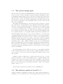
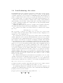
1.1
The system design goals
We started the developmentof the OcamlP3l in 1998. At that time, the main goal of
the project was to test the possibility to integrate parallel programming in a functional language using the skeleton model: after all, as we will see later, skeletons are
just functions, so a functional language should provide the natural setting for them.
We also wanted to preserve the elegance and flexibility of the functional model, and
the strong type system that comes with Ocaml. These goals were acheved in the
first version of OcamlP3l.
But during the implementation of the system, it turned out that we could get
more than that: in our implementation, the sequential semantics that is traditionally used to describe the functional behaviour of the skeletons could actually be used
to provide an elementary library allowing to execute the user code in a sequential
mode, without modifying the user code. This is a major advantage of the approach:
in our system, the user can easily debug the logic of his program running it with
the sequential semantics on a sequential machine using all the traditional techniques (including tracing and step by step execution which are of no practical use
on parallel systems), and when the program is logically correct he/she is guaranteed
(assuming the runtime we provide is correct) to obtain a correct parallel execution.
Although a similar approach has been taken in other skeleton based programming
models, by using the Ocaml programming environment this result happens to be
particularly easy to achieve. This is definitely not the case of programs written
using a sequential language and directly calling communication libraries/primitives
such as the Unix socket interface or the MPI or PVM libraries, as the logic of the
program is inextricably intermingled with low level information on data exchange
and process handling.
Following this same idea (no changes to the user code, only different semantics
for the very same skeletons), we also provided a “graphical semantics” that produces a picture of the process network used during the parallel execution of the
user program.
Finally, we wanted a simple way to generate (from the user source code) the
various executables to be run on the different nodes of a parallel machine: here
the high level of abstraction provided by functional programming, coupled with the
ability to send closures over a channel among copies of the same program provided
the key to an elementary and robust runtime system that consists of a very limited
number of lines of code.
But let’s first of all introduce the skeleton model of OcamlP3l 2.0.
1.2
The skeleton model of OcamlP3l 2.0
A skeleton parallel programming model supports so-called ‘structured parallel programming’ [6, 11, 9]. Using such a model, the parallel structure/behaviour of any
2
application has to be expressed by using skeletons picked up out of a collection
of predefined ones, possibly in a nested way. Each skeleton models a typical pattern of parallel computation (or form of parallelism) and it is parametric in the
computation performed in parallel. As an example, pipeline and farm have been
often included in skeleton collections. A pipeline just models the execution of a
number of computations (stages) in cascade over a stream of input data items.
Therefore, the pipeline skeleton models all those computations where a function
fn (fn−1 (. . . (f2 (f1 (x))) . . .)) has to be computed (the fi being the functions computed in cascade). A farm models the execution of a given function in parallel
over a stream of input data items. Therefore, farms model all those computations
where a function f (x) has to be computed independently over n input data items
in parallel.
In a skeleton model, a programmer must select the proper skeletons to program his/her application leaving all the implementation/optimization to the compiler/support. This means, for instance, that the programmer has no responsibility
in deriving code for creating parallel processes, mapping and scheduling processes on
target hardware, establishing communication frameworks (channels, shared memory
locations, etc) or performing actual interprocess communications. All these activities, needed in order to implement the skeleton application code onto the target
hardware are completely in charge to the compile/run time support of the skeleton
programming environment. In some cases, the support also computes some parameters such as the parallelism degree or the communication grain needed to optimize
the execution of the skeleton program onto the target hardware [19, 2, 20].
In the years, the skeleton model supplied by OcamlP3l has evolved. Current
OcamlP3l version (2.0) supplies three kinds of skeletons:
• task parallel skeletons, modeling parallelism exploited between independent
processing activities relative to different input data. In this set we have: pipe
(cf. 1.3.4) and farm (cf. 1.3.3), whose semantics has already been informally
described above. Such skeletons correspond to the usual task parallel skeletons
appearing both in p3l and in other skeleton models [6, 11, 13].
• data parallel skeletons, modeling parallelism exploited computing different
parts of the same input data. In this set, we provide mapvector (cf. 1.3.6)
and reducevector (cf. 1.3.7). Such skeletons are not as powerful as the map
and reduce skeletons of p3l. Instead, they closely resemble the map (∗) and
reduce (/) functionals of the Bird-Meertens formalism discussed in [3] and
the map and fold skeletons in SCL [13]. The mapvector skeleton models the
parallel application of a generic function f to all the items of a vector data
structure, whereas the reducevector skeleton models a parallel computation
folding all the elements of a vector with a commutative and associative binary
operator ⊕).
• service or control skeletons, which are not parallel per se. Service skeletons are
used to encapsulate Ocaml non-parallel code to be used within other skeletons
(seq skeleton (cf. 1.3.2)), to iterate the execution of skeletons (loop skeleton
3
(cf. 1.3.5)), to transform a process network defined using skeletons in a valid
Ocaml function (parfun skeleton (cf. 1.3.8)) and to define global application
structure (pardo skeleton (cf. 1.3.9)).
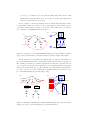
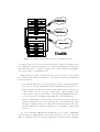
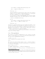
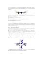
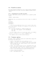
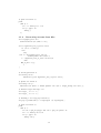
As an example, consider an application whose initial and final phase cannot
be parallelized, while the behavior in the central part is clearly divided in two
consecutive phases (stages) working on a stream of data. This can be modeled by
the combination of OcamlP3l skeletons in Fig. 1.1.
(b)
farm network
(a)
pipe
initsec
work
seq
seq
pipe
finsec
seq
work
map
reduce
seq
seq
f
g
stage2
data flow
stage1
initsecfarm
finsec
pipe network
Figure 1.1: Structure of an example OcamlP3l application: (a) the skeleton nesting,
(b) processes participating to the implementation: pardo, stage1 and stage2.
All the structure is encapsulated in a pardo skeleton. initsec and finsec are
two sequential Ocaml functions describing the initial and final parts of application.
The central part describes a parallel computation structured as a pipeline built out
of two stages. If both stages are implemented via a sequential function (seq) data
will flow as shown in Fig. 1.1.(a). In particular, the implementation spawns three
processes: a ‘pardo’ process (executing the sequential parts) and a network of two
processes implementing the pipeline (Fig. 1.1.(b)).
(a)
(b)
pardo
init
init
dfarm
dfarm
dataflow
farm network
hfun
dpipe
stage1
hfun
final
dpipe
parfun
parfun
final
pipe
pardo
seq
seq
seq
r
g
f
stage2
dfarm
farm
work
pipe network
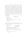
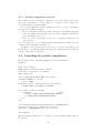
Figure 1.2: Further parallelizing the example OcamlP3l application: (a) the skeleton
nesting, (b) the processes participating to the implementation.
4
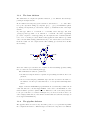
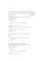
Now, suppose the programmer recognizes that the initsec is computationally
intensive and can be decomposed in a sequential part (initsec) and a parallel
part which applies a function work independently on each element on a stream of
input data. In this case, we can use a farm skeleton to have a pool of replicas of
work. Moreover, suppose the function stage1 boils down to applying a function f
to all the elements of a vector and function stage2 “sums” up all the elements of
the resulting vector by using an associative and commutative operator g. In this
case, the programmer can refine the skeleton structure by using the combination
in Fig. 1.2. Here, the four replicas of work act on different independent elements
in the input stream, producing four stream of results (vectors) which are merged
before entering the pipeline. Each stage is in turn implemented in parallel using
four processes. In the first stage, each input vector is partitioned into four blocks.
Each process takes care of applying f on one of the four blocks. Then in the second
stage, each process sums up the elements in a block of the vector and then all the
partial results are added before providing the final result back to the pardo (and to
the finsec function).
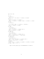
The first “application outline” (Fig. 1.1) corresponds to the following (incomplete) OcamlP3l code:
let initsec _ = ...;;
(* generates stream *)
let finsec x = ...;;
(* consumes stream *)
let stage1 _ x = ... ;;
let stage2 _ x = ... ;;
(* defines pipe network *)
let pipe = parfun (fun () -> seq(stage1) ||| seq(stage2)) ;;
pardo (fun () ->
let y = pipe (initsec ()) in
finsec y
);;
notice the use of seq skeleton to encapsulate ordinary Ocaml functions and the use
of parfun to define the pipe network. Here is the sketch of OcamlP3l code for the
second application outline (Fig. 1.2):
let degree = ref 4;
(* parallel degree *)
let work _ x = ..;;
(* to be farmed out *)
let f _ x = ...;;
(* to be mapped *)
let g _ (x,y) = ...;;
(* to be reduced *)
let pstage1 = mapvector(seq(f),!degree);;
let pstage2 = reducevector(seq(g),!degree);;
let pipe = parfun (fun () -> pstage1 ||| pstage2);;
let afarm = parfun (fun () -> farm (seq(farm_worker),!degree));;
pardo
(fun () ->
let y = pipe (afarm (initsec ())) in
finsec y
);;
5
here !degree refers to the number of parallel processes to be used in the skeleton
implementation of mapvector, reducevector and farm. This value can vary in each
execution of the application without recompiling (eg., using a configuration file).
Details on how to write and run proper OcamlP3l programs are given later in Chapter 2. In the current release, the user is supposed to explicitly give the number of
processors to be used in each farm, mapvector and reduce skeleton. In other words
the choice of the parallelism degree actually exploited in such skeletons is up to the
programmer. It is foreseeable in a future release to ask the system to guess optimal
values depending on available resources (following the approach of p3l [2, 19]), as it
is discussed in more detail below.
Applications with a parallel structure given by skeletons (such as the ones outlined above) can be implemented by using implementation templates [6, 19]. An
implementation template is a known, parametric way of exploiting the kind of parallelism modeled by a skeleton onto a particular target architecture. As an example,
a template corresponding to the mapvector skeleton will take some input vector
data, it will split the data into chunks holding one or more data items of the vector,
schedule them to a set of “worker” processes computing the map function f and
finally collect the results and rebuild the output vector data structure. All these
operations will be performed by some processes, using either communications or
shared memory locations for data communication. Such a template must, as its
primary goal, implement in an efficient way the mapvector skeleton and therefore:
• it must implement any kind of mapvector function f , and therefore must be
parametric with respect to the input and output data types
• it must support any reasonable parallelism degree, therefore it must work
(and provide effective parallelism exploitation) when executed on an arbitrary
number of processors.
In OcamlP3l 2.0, the parallelism degree of each skeleton is chosen by the programmer. In following releases, we will explore the possibility of using analytic
performance models associated with the implementation template process networks
to derive the parallelism degree automatically[21]. An analytic performance model
is a set of functions computing different measures of the performance achieved by
a template on the basis of a small set of machine dependent and user code parameters. Examples of machine dependent parameters are the cost of communication
startup and the per-byte transmission cost. Examples of user code parameters are
the mean and variance of execution time for user-defined sequential parts of the
program and the size of data flowing between skeletons. The models describe the
template behavior as a function of the resources used (e.g. the physical number
of executors in a farm) and can be used by the skeleton support to predict such
behavior and to tune resource allocation. A more detailed description of the whole
automatic optimization process executed by a compiler using performance models
for skeleton tuning is given in [19, 20, 21].
6
1.2.1
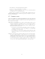
Parallel execution model
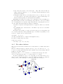
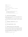
A parallel computation in OcamlP3l is defined by three components:
• a set of plain sequential Ocaml functions (CF, common functions in Figure 1.3),
• some clusters of parallel processes, each one defined by a suitable composition of skeleton combinators enclosed in a parfun (SF, skeleton functions in
Figure 1.3) and
• a pardo application.
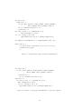
Each time a parfun(h) functon definition is evaluated, a corresponding network
of processes is created according to the skeleton composition in h. Each network
transforms a stream of independent input data . . . x1 , x0 in a stream of output data
. . . h(x1 ), h(x0 ) according to h.
When a pardo is evaluated, applications of common functions boil down to
normal sequential evaluation, while applications of skeletal functions feed arguments
data to the corresponding skeletal process network and are evaluated in parallel.
In practice, each pardo defines a network built out of all the processes in skeletal
networks (parfun defined functions) plus a root process orchestrating all the computation. Both the root node and the generic nodes run in SPMD model. Initially,
the root specializes all the generic nodes sending information on the actual process
to be executed (eg., a farm dispatcher, a farm worker, a mapvector worker etc).
Then, the root process starts executing the pardo. If code is sequential, it is
executed locally on the root node. Otherwise, if the evaluation of a parfun function
is encountered, the root activates evaluation passing the relevant parameters to the
correponding network. The same network can be activated many times, each time
an evaluation of the corresponding parfun function is encountered.
Notice that the execution model assumes an unlimited number of homogenous
processors. In practical situations, processors will be less than processes and have
heterogeneus capacity. The OcamlP3l upport, possibly with some help from the
programmer (using colors, see Sec. 1.4), is in charge of implementing this in a
transparent way.
1.2.2
Discussion: a comparision with p3l
Even if OcamlP3l skeletons are close to original p3l ones, the parallel evaluation
model is completely different. Thus, for these familiar with p3l, it is interesting to
highlight the main differences between two models and to give a brief account on
the reasons that have lead to such a design change.
In the original p3l system (and, actually in initial versions of OcamlP3l[10]), a
program is clearly stratified into two levels: there is a skeleton cap, that can be
composed of an arbitrary number of skeleton combinators, but as soon as one goes
outside this cap, passing into the sequential code through the seq combinator, there
is no way for the sequential code to call a skeleton. To say it briefly, the entry point
7
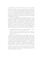
Figure 1.3: Parallel execution model: the role of parfun and pardo
of a p3l program must be a skeleton expression, and no skeleton expression is allowed anywhere else in the sequential code. Using current OcamlP3l terminology,
p3l restricts the pardo to contain one single call to a network defind with parfun,
and without calls to sequential functions.
This restriction is quite reasonable when the goal is to build a single stream
processing network described by the skeleton cap. However, it has several drawbacks
in the general case:
• it breaks uniformity, since even if the skeletons look like ordinary functionals,
they cannot be used as ordinary functions, in particular inside sequential code,
• many applications (such as the numerical algorithms described in [5]) boil
down to simple nested loops, some of which can be easily parallelised, and
some cannot; forcing the programmer to push all the parallelism in the skeleton cap could lead to rewriting the algorithm in a very unnatural way,
• indeed, a ‘parallelizable’ operation can be used at several stages in the algorithm: the p3l skeleton cap does not allow the user to specify that parts of the
stream processing network can be shared among different phases of the computation, which is an essential requirement to avoid wasting computational
resources.
To overcome all these difficulties and limitations, the 2.0 version of OcamlP3l
introduces the new parfun skeleton (not present in p3l), the very dual of the seq
skeleton. In simple words, one can wrap a full skeleton expression inside a parfun,
8
(* computes x square *)
let farm_worker _ = fun x -> x *. x;;
(* prints a result *)
let print_result x = print_float x; print_newline();;
let compute = parfun (fun () ->
(farm (seq(farm_worker),4)));;
pardo(fun () ->
let is = P3lstream.of_list [1.0;2.0;3.0;4.0;5.0;6.0;7.0;8.0] in
let s’ = compute is in P3lstream.iter print_result s’;
);;
Figure 1.4: OcamlP3l code using a farm to square a stream of float.
and obtain a regular Ocaml stream processing function, usable with no limitations
in any sequential piece of code: a parfun encapsulated skeleton behaves exactly as
a normal function that receives a stream as input, and returns a stream as output.
However, in the parallel semantics, the parfun combinator gets a parallel interpretation, so that the encapsulated function is actually implemented as a parallel
network (the network to which the parfun combinator provides an interface).
Since many parfun expressions may occur in an OcamlP3l program, there may be
several disjoint parallel processing networks at runtime. This implies that, to contrast with p3l, the OcamlP3l model of computation requiers a main sequential program (the pardo): this main program is responsible for information interchange
with the various parfun encapsulated networks.
1.2.3
A simple example: farming square computation
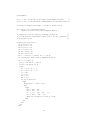
It is now time to discuss a simple but complete OcamlP3l program. The program
in Figure 1.4 uses a farm to compute a very simple function over a stream of
floats. First we have two standard Ocaml functions: farm_worker which simply
computes the square of a float argument and print_result which dumps results
on the stardard output. Notice that farm_worker takes two parameters instead
of one as it would seem reasonable. The extra parameter (_) is required by the
seq skeleton type and is used in general to provide local initialization data (for
instance, an initialization matrix, some initial seed or the like). In this simple case,
initialization data are not needed and the parameter is just ignored by farm_worker.
This optional initialization is provided for all OcamlP3l skeletons (see Section 1.3.1).
Function compute uses parfun to define a parallel network built by a single farm,
in particular:
seq(farm_worker)
turns the sequential farm_worker function into a ‘stream processor’ applying it to
a stream of input values. Then, an instance of the farm skeleton is defined with
9
farm (seq(farm_worker),4)
which spawns four workers. Finally,
parfun (fun () ->
(farm (seq(farm_worker),4)));;
encapsulates the skeleton network into a standard Ocaml function.
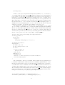
The last pardo defines how sequential functions and parallel modules are interconnected. In this case, we have a single parallel module (compute) and two
sequential parts. The first sequential part builds up the data stream (using the
standard OcamlP3l library function
P3lstream.of_list [1.0;2.0;3.0;4.0;5.0;6.0;7.0;8.0]
which turns lists in streams) and the second part applies print_results to all
the elements in the stream (using standard stream iterator P3lstream.iter). The
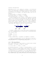
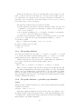
global network is shown in Figure 1.5, where arrows point out the data flow among
processes.
compute
farm_worker
P3lstream.of_list...
P3lstream.iter...
pardo
Figure 1.5: Overall process network of the simple farm squaring a stream of double.
1.3
Skeleton syntax, semantics, and types
Here we describe the syntax, the informal semantics, and the types assigned to each
skeleton combinator.
Each skeleton is a stream processor, transforming an input stream into an output
stream and is equipped with three semantics:
sequential semantics a suitable sequential Ocaml function transforming all the
elements of the input stream;
parallel semantics a process network implementing the stream transformation in
parallel;
graphical semantics a graphical representation of the process network corresponding to the parallel semantics.
10
1.3.1
On the type of skeleton combinators
First of all, let’s explain why the actual Ocaml types of our skeleton combinators are
a bit more complex than those used by other skeleton systems (eg., [13]). In effect,
our types seem somewhat polluted by spurious additional unit types, compared to
the types one would expect.
For istance, consider the seq combinator. As informally discussed above, seq
encapsulates any Ocaml function f into a sequential process which applies f to
all the inputs received in the input stream. This means that, writing seq f, any
Ocaml function with type f : ’a -> ’b is wrapped into a sequential process (this
is reminiscent to the lift combinator used in many stream processing libraries of
functional programming languages).
Hence, a strightforward type for seq would be
(’a -> ’b) -> ’a stream -> ’b stream.
However, in OcamlP3l, seq is declared as
seq : (unit -> ’a -> ’b) -> unit -> ’a stream -> ’b stream
meaning that the lifted function argument f gets an extra unit argument. In effect,
in real-world application, the user functions may need to hold a sizeable amount
of local data (e.g. some huge matrices that have to be initialised in a numerical
application), and we decided to have a type general enough to allow the user to
finely describe where and when those data have to be initialized and/or copied.
Reminiscent to partial evaluation and λ-lifting, we reuse the classical techniques
of functional programming to initialize or allocate data globally and/or locally to a
function closure. This is just a bit complicated here, due to the higher-order nature
of the skeleton algebra, that in turn reflects the inherent complexity of parallel
computing:
• global initialization: the data is initialised once and for all, and is then replicated in every copy of the stream processor that a farm, a mapvector or a
reducevector may launch; this was already available in the previous versions
of OcamlP3l, since we could write
let f =
let localdata = do_huge_initialisation_step () in
fun x -> compute (localdata, x);;
...
farm (seq f, 10)
• local initialization: the data is initialised by each stream processor, after the
copy has been performed by a farm or a mapvector skeleton; this was just
impossible in the previous versions of OcamlP3l; with unit types, it is now
easy to achieve:
let f () =
11
let localdata = do_huge_initialisation_step () in
fun x -> compute (localdata, x);;
...
farm (seq f, 10)
when the farm skeleton creates 10 copies of seq f, each copy is created by
passing () to the seq combinator, which in turn passes () to f , producing the
allocation of a different copy of localdata for each instance4 .
Note also that the old behaviour, namely OcamlP3l version 1.0, where a unique
initialization was shared by all copies, is still easy (and can be freely combined
to further local initializations if needed):
let f =
let localdata = do_huge_initialisation_step () in
fun () -> fun x -> compute (localdata, x);;
...
farm (seq f, 10)
To sum up, the extra unit parameters give the programmer the hability to decide
whether local initialisation data in his functions are shared among all copies or not.
In other words, we can regard the skeleton combinators in the current version of
OcamlP3l as “delayed skeletons”, or “skeleton factories”, that produce an instance
of a skeleton every time they are passed an () argument.
In the following sections we detail the types and semantics of all the skeletons
and provide some usage examples.
1.3.2
The seq skeleton
The seq skeleton encapsulates an Ocaml function f into a stream process which
applies f to all the inputs received on the input stream and sends off the reselts on
the output stream. Any Ocaml function with type
f: unit -> ’a -> ’b
can be encapsulated in the seq skeletons as follows:
seq f
The central point is that the function must be unary, i.e. functions working on
more that one argument must collect them in a single tuple before being used in a
seq. For instance, the fragment
let g _ (x,y) = x *. y;;
let redmul = parfun (fun () -> reducevector(seq(g),6));;
shows how to encapsulate a float binary operator (*.) to use it within a reducevector
with 6 working processes.
4 In
practice, the initialization step may do weird, non referentially transparent things, like
opening file descriptors or negociating a network connection to other services: it is then crucial
to allow the different instances of the user’s function to have their own local descriptors or local
connections to simply avoid the chaos.
12
1.3.3
The farm skeleton
The farm skeleton computes in parallel a function f over different data items appearing in its input stream.
From a functional viewpoint, given a stream of data items x1 , . . . , xn , and a function f , the expression farm(f, k) computes f (x1 ), . . . , f (xn ). Parallelism is gained
by having k independent processes that compute f on different items of the input
stream.
If f has type (unit -> ’b stream -> ’c stream), and k has type int, then
f arm(f, k) has type unit -> ’b stream -> ’c stream. In terms of (parallel)
processes, a sequence of data appearing onto the input stream of a farm is submitted to a set of worker processes. Each worker applies the same function (f , which
can be in turn difined using parallel skeletons) to the data items received and delivers the result onto the output stream. The resulting process network looks like
the following:
#$# "! $# "! $# Worker
"! $# #### $$$$#### ""!!"!"! $$$$#### ""!!"!"! $$$$#### ""!!"!"! $$$$#### #### $$$$#### "!"!"! $$$$#### "!"!"! $$$$#### "!"!"! $$$$#### ###$$$### "!"!"! $$$### "!"!"! $$$### "!"!"! $$$### ### $$$### "!"! $$$### "!"! $$$### "!"! $$$### ### $$$### $$$### $$$### $$$### Output
Input data
data
####$$$$#### $$$$#### $$$$#### $$$$#### ###$$$### $$$### $$$### $$$### ##$$## $$## $$## $$## Emitter
Collector
###$$$### $$$### $$$### $$$###
where the emitter process takes care of task-to-worker scheduling (possibly taking
into account some load balancing strategy).
The farm function takes two parameters:
• the first denoting the skeleton expression representing the farm worker computation,
• the second denoting the parallelism degree the user decided for the farm, i.e.
the number of worker processes that have to be set up in the farm implementation.
Figure 1.6 shows an OcamlP3l program which chooses randomly a number from
a list and writes it to the file magic number. Notice the local initialization of the
random number generator (which takes a different seed in each worker) and the
local open of the file to be written. In Figure 1.7 you can see how the worker code
can be simply transformed to have all the workers share the same filed descripto if
needed (global initialization).
1.3.4
The pipeline skeleton
The pipeline skeleton is denoted by the infix operator |||; it performs in parallel
the computations relative to different stages of a function composition over different
13
let write_int =
function () ->
let fd = Unix.openfile "magic_number" [Unix.O_WRONLY;
Unix.O_CREAT; Unix.O_TRUNC] 0o644 in
let () = Random.self_init () in
( function x ->
let time_to_wait = 1 + (Random.int 3) in
Unix.sleep(time_to_wait);
let sx = string_of_int x in
ignore(Unix.write fd sx 0 (String.length sx));;
let parwrite = parfun(fun () -> farm(seq(write_int), 5));;
pardo( fun () ->
let the_stream = P3lstream.of_list [0;1;2;3;4] in
parwrite the_stream
);;
Figure 1.6: A simple farm example (with local initialization)
let write_int =
let fd = Unix.openfile "magic_number" [Unix.O_WRONLY;
Unix.O_CREAT; Unix.O_TRUNC] 0o644 in
( function () ->
let () = Random.self_init () in
function x ->
let time_to_wait = 1 + (Random.int 3) in
Unix.sleep(time_to_wait);
let sx = string_of_int x in
ignore(Unix.write fd sx 0 (String.length sx));;
Figure 1.7: Worker code using global initialization to share file descriptor
14
data items of the input stream.
Functionally, f1 |||f2 . . . |||fn computes fn (. . . f2 (f1 (xi )) . . .) over all the data
items xi in the input stream. Parallelism is now gained by having n independent parallel processes. Each process computes a function fi over the data items
produced by the process computing fi−1 and delivers its results to the process computing fi+1 .
If f1 has type (unit -> ’a stream -> ’b stream),
and f2 has type (unit -> ’b stream -> ’c stream),
then f1 |||f2 has type unit -> ’a stream -> ’c stream.
In terms of (parallel) processes, a sequence of data appearing onto the input
stream of a pipe is submitted to the first pipeline stage. This stage computes the
function f1 onto every data item appearing onto the input stream. Each output
data item computed by the stage is submitted to the second stage, computing the
function f2 and so on and so on until the output of the n − 1 stage is submitted to
the last stage. Eventually, the last stage delivers its own output onto the pipeline
output channel. The resulting process network looks like the following:
f1
f2
Input data
stage1
stage2
fn
Output
data
stagen
For instance, a pipeline made out of three stages, the first one squaring integers,
the second one multiplying integers by 2 and the third one incrementing integers
can be written as follows:
let
let
let
let
square _ x = x
double _ x = 2
inc
_ x = x
apipe = parfun
* x;;
* x;;
+ 1;;
(fun () -> seq(square) ||| seq(double) ||| seq(inc));;
A pipeline models (parallel) function composition, thus input and output types of
stages should match. This means that if stage (i − 1) has type unit -> ’c -> ’a stage
(i + 1) has type unit -> ’b -> ’d stage i-th must have type unit -> ’a -> ’b.
1.3.5
The loop skeleton
The loop skeleton named loop; it computes a function f over all the elements of its input
stream until a boolean condition g is verified. A loop has type
(’a -> bool) * (unit -> ’a stream -> ’a stream)
provided that f has type unit -> ’a stream -> ’a stream and g has type ’a -> bool.
Function f is computed before testing termination, thus it is applied at least one time to
each input stream element. In terms of (parallel) processes, a sequence of data appearing
onto the input stream of a loop is submitted to a loop in stage. This stage just merges
data coming from the input channel and from the feedback channel and delivers them to
the loop body stage. The loop body stage computes f and delivers results to the loop end
stage. This latter stage computes g and either delivers (f x) onto the output channel (in
15
case (g (f x)) turns out to be true) or it delivers the value to the loop in process along
the feedback channel ((g (f x)) = false). The resulting process network looks like the
following:
loop in
Input data
f
loop out
Output data
g
For instance, the following loop increments all the integer data items in the input stream
until they become divisible by 5:
let notdivbyfive x = (x mod 5 <> 0);;
let inc _ x = x + 1;;
let aloop = parfun (fun () -> loop(notdivbyfive,seq(inc)));;
The output of this function on the sequence
3,7,10,14
is 5,10,15,15. In particular, the call theloop 10 returns 15 as the body seq(inc) is
evaluated on input data before the condition, and therefore the first time the condition is
evaluated on 11 and not on 10.
1.3.6
The map skeleton
The map skeleton is named mapvector; it computes in parallel a function over all the data
items of a vector, generating the (new) vector of the results.
Therefore, for each vector X in the input data stream, mapvector(f, n) computes the
function f over all the items of X = [x1 , . . . , xn ], using n distinct parallel processes that
compute f over distinct vector items ([f (x1 ), . . . , f (xn )]).
If f has type (unit -> ’a stream -> ’b stream), and n has type int, then mapvector(f, n)
has type unit -> ’a array stream -> ’b array stream.
In terms of (parallel) processes, a vector appearing onto the input stream of a mapvector is split n elements and each element is computed by one of the n workers. Workers
apply f to the elements they receive. A collector process is in charge of gluing together
all the results in a single result vector.
#$# "! $# "! $# Worker
"! $# #### $$$$#### "!"!"!"! $$$$#### "!"!"!"! $$$$#### "!"!"!"! $$$$#### #### $$$$#### "!!""! $$$$#### "!!""! $$$$#### "!!""! $$$$#### ###$$$### "!"!"! $$$### "!"!"! $$$### "!"!"! $$$### ### $$$### "!"! $$$### "!"! $$$### "!"! $$$### ### $$$### $$$### $$$### $$$### Output
Input data
###$$$### $$$### $$$### $$$### data
###$$$### $$$### $$$### $$$### ###$$$### $$$### $$$### $$$### Emitter
Collector
###$$$### $$$### $$$### $$$###
Different strategies can be used to distribute a vector [|x1;...;xm|] appearing in the
input data stream to the workers. As an example the emitter:
16
• may round robin each xi to the workers ({w1,...wn}). The workers in this case
simply compute the function f :0 a →0 b over all the elements appearing onto their
input stream (channel).
• may split the input data vector in exactly n sub-vectors to be delivered one to each
one of the worker processes. The workers in this case compute an Array.mapf over
all the elements appearing onto their input stream (channel).
Summarizing, the emitter process takes care of (sub)task-to-worker scheduling (possibly implementing some kind of load balancing policy), while the collector process takes
care of rebuilding the vector with the output data items and of delivering the new vector
onto the output data stream. mapvector takes two arguments:
• the skeleton expression denoting the function to be applied to all the vector elements,
and
• the parallelism degree of the skeleton, i.e. the number of processes to be used in the
implementation.
For instance, the following code works on a stream of integer vectors and squares each
vector element. The skeleton has a parallelism degree of 10, that is ten parallel processes
are used to compute each vector in the stream.
let square _ x = x * x;;
let amap = parfun (fun () -> mapvector(seq(square),10));;
the result on a single array is as follows
# amap [|1;2;3;4;5|];;
- : int array = [|1; 4; 9; 16; 25|]
1.3.7
The reduce skeleton
The reduce skeleton is named reducevector; it folds a function over all the data items of
a vector.
Therefore, reducevector(⊕, n) computes x1 ⊕ x2 ⊕ . . . ⊕ xn out of the vector x1 , . . . , xn ,
for each vector in the input data stream. The computation is performed using n different
parallel processes that compute f .
If ⊕ has type (unit -> ’a * ’a stream -> ’a stream), and n has type int, then
reducevector(⊕, n) has type unit -> ’a array stream -> ’a stream.
In terms of (parallel) processes, a vector appearing onto the input stream of a reducevector is processed by a logical tree of processes. Each process is able to compute the
binary operator g. The resulting process network looks like the following tree:
Input data
Emitter
Worker processes
g
17
Output data
In this case, the emitter process is the one delivering either couples of input vector data
items or couples of sub-vectors of the input vector to the processes belonging to the tree
base. In the former case, log(n) levels of processes are needed in the tree, in the latter one,
any number of process levels can be used, and the number of sub-vectors to be produced
by the emitter can be devised consequently.
The reducevector function takes two parameters as usual:
• the first parameter is the skeleton expression denoting the binary, associative and
commutative operation (these properties must be ensured by the programmer to
have a correct execution)
• the second is the parallelism degree, i.e. the number of parallel processes that have
to be set up to execute the reducevector computation.
For instance, the following skeleton instance accepts in input a stream of vectors and,
for each vector, computes the sum of all elements using the arithmetic + operator.
let areduce = parfun
(fun () -> reducevector(seq(fun _ (x,y) -> x + y),10));;
the result on a single array is as follows
# areduce [|1;2;3;4|];;
- : int = 10
1.3.8
The parfun skeleton
One would expect parfun to have type (unit -> ’a stream -> ’b stream) -> ’a stream
-> ’b stream: given a skeleton expression with type (unit -> ’a stream -> ’b stream),
parfun returns a stream processing function of type ’a stream -> ’b stream.
parfun’s actual type introduces an extra level of functionality: the argument is no
more a skeleton expression but a functional that returns a skeleton:
val parfun :
(unit -> unit -> ’a stream -> ’b stream) -> ’a stream -> ’b stream
This is necessary to guarantee that the skeleton wrapped in a parfun expression will
only be launched and instanciated by the main program (pardo), not by any of the multiple
running copies of the SPMD binary, even though thoses copies may evaluate the parfun
skeletons; the main program will actually create the needed skeletons by applying its
functional argument, while the generic copies will just throw the functional away, carefully
avoiding to instanciate the skeletons.
1.3.9
The pardo skeleton: a parallel scope delimiter
Typing
Finally, the pardo combinator defines the scope of the expressions that may use the parfun
encapsulated expressions.
val pardo : (unit -> ’a) -> ’a
pardo takes a thunk as argument, and gives back the result of its evaluation. As for
the parfun combinator, this extra delay is necessary to ensure that the initialization of the
code will take place exclusively in the main program and not in the generic SPMD copies
that participate to the parallel computation.
18
Parallel scoping rule
In order to have the parfun and pardo work correctly together the following scoping rule
has to be sollowed:
• functions defined via the parfun combinator must be defined before the occurrence
of the pardo combinator,
• those parfun defined functions can only be executed within the body of the functional
parameter of the pardo combinator,
• no parfun can be used directly inside a pardo combinator.
Structure of an OcamlP3l program
Due to the scoping rule in the pardo, the general structure of an OcamlP3l program looks
like the following:
(* (1) Functions defined using parfun *)
let f = parfun(skeleton expression )
let g = parfun(skeleton expression )
(* (2) code referencing these functions under abstractions *)
let h x = ... (f ...) ... (g ...) ...
...
(* NO evaluation of code containing a parfun is allowed outside pardo *)
...
(* (3) The pardo occurrence where parfun encapsulated
functions can be called. *)
pardo
(fun () ->
(* NO parfun combinators allowed here *)
(* code evaluating parfun defined functions *)
...
let a = f ...
let b = h ...
...
)
(* finalization of sequential code here *)
At run time, in the sequential model, each generic copy just waits for instructions from
the main node; the main node first evaluates the arguments of the parfun combinators
to build a representation of the needed skeletons; then, upon encountering the pardo
combinator, the main node initializes all the parallel computation networks, specialising
the generic copies (as described in details in [10]), connects these networks to the sequential
interfaces defined in the parfun’s, and then runs the sequential code in its scope by applying
its function parameter to ():unit. The whole picture is illustrated in Figure 1.3. The
skeleton networks are initiated only once but could be invoked many times during the
execution of pardo.
19
1.4
Load balancing: the colors
In the OcamlP3l system, the combinators expressions govern the shape of the process network and the execution model assumes a ‘virtual’ processor, for each process. The mapping
of virtual to physical processors is delegated to the OcamlP3l system. The mapping is currently not optimized in the system. However, programs and machines can be annotated
by the programmer using colors, which can pilote the virtual-to-physical mapping process.
The idea is to have the programmer to rank the relative ‘weight’ of skeleton instances
and the machine power in a range of integer values (the colors). Then, weights are used
to generate a mapping in which load is evenly balanced on the partecipating machine
according to their relative power.
Pushing the difficult part of the generaion of weights to the programmer’s knowledge
and ability, this simple and practical idea gives surprisingly good results in practice.
Let’s consider as an example, the skeletal expression we discussed in the example
(Sec 1.2.3):
farm (seq (f un x → x ∗ x), 16)
that corresponds to a network of one emitter node, one collector node, and 16 worker
nodes which compute the square function. There are numerous ways of mapping a set of
virtual nodes to a set of physical nodes.
If no information is provided, the support uses a simple round robin, which maps
virtual to physical nodes in a cyclic way: first all phisical processors get one process then
we start again from the beginning until virtual processors are all allocated. Unfortunately,
such a solution doesn’t take into account the load balancing constraints: all the physical
(resp. virtual) nodes are considered equivalent in computing power and are used evenly.
If the programmer knows more about machines and processes he/she can tell the system
using colors. A color is an optional integer parameter that is added to OcamlP3l expressions
in the source program and to the execution command line of the compiled program. We
use the regular Ocaml’s optional parameters syntax, with keyword col, to specify the colors
of a network of virtual nodes. For example, writing farm ~col:k (f, n) means that all
virtual nodes inside this farm structure should be mapped to some physical nodes with a
capability ranking k. The scope of a color specification covers all the inner nodes of the
structure it qualifies: unless explicitely specified, the color of an inside expression is simply
inherited from the outer layer (the outermost layer has a default color value of 0 which
means no special request).
For combinators farm, mapvector and reducevector, in addition to the color of the
combinator itself, their is an additional optional color parameter colv. A colv[ ] specification is a color list (i.e. an int list) that specifies the colors of the parallel worker
structures that are arguments of the combinator. As an example, the OcamlP3l expression
map ~col:2 ~colv:[ 3; 4; 5; 6 ] (seq f, 4)
is a mapvector skeleton expression, with emitter and collector nodes of rank 2, and four
worker nodes (four copies of seq f) whith respective ranks 3, 4, 5, and 6.
To carefully map virtual nodes to physical nodes, we also need a way to define the colors
of physical nodes. This information is specified on the command line when launching the
program (see Section 2). One can write:
prog.par -p3lroot ip1:port1#color1 ip2:port2#color2 ... \
ip i:port i#color i ...
20
where ip i:port i#color i indicates the ip address (or name), the port, and the color of
the physical node i participating to the computation. The port and color here are both
optional. With no specified port, a default p3lport is used; with no color specification, the
default color 0 is assumed.
If the colors of all the virtual processors and all the physical processors have a one-toone correspondance, the mapping is easy. But such a perfect mapping does not exist in
general: first of all, there is not always equality between the amount of physical processors
we have and the amount of virtual processors we need; second, in some very complex
OcamlP3l expressions, it is complex and boring for the programmer to calculate manually
how many virtual nodes are needed for each color class.
So, we decided to use a simple but flexible mapping algorithm, based on the idea that
what a color means is not the exact capability required but the lowest capability acceptable.
For example, a virtual node with color value 5 means a physical node of color 5 is needed,
but if there is no physical node with value 5, and there exists a physical node of color 6
free and available, why don’t we take it instead? In practice, we sort the virtual nodes in
decreasing order of their color values, to reflect their priority in choosing a physical node:
virtual nodes with bigger colors should have more privilege and choose their physical node
before the nodes with smaller colors. Then, for each virtual node, we lists all the physical
nodes with a color greater than or equal to the virtual node color. Among all those qualified
ones, the algorithm finally associates the virtual node with the qualified node which has
the smallest work load (the one that has the least number of virtual nodes that have been
assigned to it).
This algorithm provides a mapping process with some degree of automatization and
some degree of manual tuning, but one has to keep in mind that the color designs a
computational class, qualitatively, and is not an exact quantitative estimation of the computational power of the machine, as the current version of OcamlP3l does not provide yet
the necessary infrastructure to perform an optimal mapping based on precise quantitative
estimations of the cost of each sequential function and the capabilities of the physical nodes,
so that we cannot guarantee our color-based mapping algorithm to be highly accurate or
highly effective.
Still, the “color” approach is accurate and simple enough to be quite significant to the
programmer: according to the experiments we have conducted, it indeed achieved some
satisfactory results in our test bed case (see [5]).
Figure 1.8 summarizes the types of the combinators, exactly as they are currently
available to the programmer in the 2.0 version of OcamlP3l, including the optional color
parameters.
21
type color = int
val seq :
?col:color ->
(unit -> ’a -> ’b) -> unit -> ’a stream -> ’b stream
val ( ||| ) :
(unit -> ’a stream -> ’b stream) ->
(unit -> ’b stream -> ’c stream) -> unit -> ’a stream -> ’c stream
val loop :
?col:color ->
(’a -> bool) * (unit -> ’a stream -> ’a stream) ->
unit -> ’a stream -> ’a stream
val farm :
?col:color ->
?colv:color list ->
(unit -> ’b stream -> ’c stream) * int ->
unit -> ’b stream -> ’c stream
val mapvector :
?col: color ->
?colv:color list ->
(unit -> ’b stream -> ’c stream) * int ->
unit -> ’b array stream -> ’c array stream
val reducevector :
?col:color ->
?colv:color list ->
(unit -> (’b * ’b) stream -> ’b stream) * int ->
unit -> ’b array stream -> ’b stream
val parfun :
(unit -> unit -> ’a stream -> ’b stream) -> ’a stream -> ’b stream
val pardo : (unit -> ’a) -> ’a
Figure 1.8: The (complete) types of the OcamlP3l skeleton combinators
22
Chapter 2
Running your OcamlP3l
program
We give here a practical tutorial on how to use the system, without entering into the
implementation details of the current version of OcamlP3l.
As mentioned above, once you have written an OcamlP3l program, you have several
choices for its execution, since you can without touching your source:
sequential run your program sequentially on one machine, to test the logic of the algorithm you implemented with all the usual sequential debugging tools.
graphics get a picture of the processor net described by your OcamlP3lskeleton expression
to grasp the parallel structure of your program.
parallel run your program in parallel over a network of workstations after a simple recompilation.
Presumably, you would run the parallel version once the program has satisfactorily passed
the sequential debugging phase.
In the following sections, our running example is the computation of a Mandelbrot
fractal set. We will describe the implementation program, compile it and run it in the
three ways described above.
2.1
The Mandelbrot example program
The Mandelbrot example program performs the calculation of the Mandelbrot set at a
given resolution in a given area of the graphic display. This is the actual program provided
in the Examples directory of the distribution.
The computing engine of the program is the function pixel row which computes the
color of a row of pixels from the convergence of a sequence of complex numbers zn defined
by the initial term z0 and the formula zn+1 = zn2 + z0 . More precisely, given a point
p in the complex plane, we associate to p the sequence zn when starting with z0 = p.
Now, we compute the integer m such that zm is the first term of the sequence satisfying
the following condition: either the sum of the real and imaginary parts of zn exceeds a
given threshold, or the number of iterations exceeds some fixed maximum resolution limit.
Integer m defines the color of p.
p). This correspond to the following Ocaml code:
23
open Graphics;;
let n
= 300;; (* the size of the square screen windows in pixels
*)
let res = 100;; (* the resolution: maximum number of iterations allowed *)
(* convert an integer in the range 0..res into a screen color *)
let color_of c res = Pervasives.truncate
(((float c)/.(float res))*.(float Graphics.white));;
(* compute the color of a pixel by iterating z_m+1=z_m^2+c
*)
(* j is the k-th row, initialized so that j.(i),k are the coordinates *)
(* of the pixel (i,k)
*)
let pixel_row (j,k,res,n) =
let zr = ref 0.0 in
let zi = ref 0.0 in
let cr = ref 0.0 in
let ci = ref 0.0 in
let zrs = ref 0.0 in
let zis = ref 0.0 in
let d
= ref (2.0 /. ((float n) -. 1.0)) in
let colored_row = Array.create n (Graphics.black) in
for s = 0 to (n-1) do
let j1 = ref (float j.(s)) in
let k1 = ref (float k) in
begin
zr := !j1 *. !d -. 1.0;
zi := !k1 *. !d -. 1.0;
cr := !zr;
ci := !zi;
zrs := 0.0;
zis := 0.0;
for i=0 to (res-1) do
begin
if(not((!zrs +. !zis) > 4.0))
then
begin
zrs := !zr *. !zr;
zis := !zi *. !zi;
zi := 2.0 *. !zr *. !zi +. !ci;
zr := !zrs -. !zis +. !cr;
Array.set colored_row s (color_of i res);
end;
end
done
end
done;
24
(colored_row,k);;
In this code, the global complex interval sampled stays within (-1.0, -1.0) and (1.0,
1.0). In this 2-unit wide square, the pixel row functions computes rows of pixels separated
by the distance d. The pixel row function takes four parameters: size, the number of
pixels in a row; resolution, the resolution; k, the index of the row to be drawn; and, j,
an array which will be filled with the integers representing the colors of pixels in the row.
These values will be converted into real colors by the color row function. In this program,
the threshold is fixed to be 4.0. We name zr and zi the real and imaginary parts of zi ;
similarly, the real and imaginary parts of c are cr and ci; zrs and zis are temporary
variables for the square of zr and zi; d is the distance between two rows.
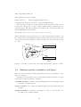
The Mandelbrot computation over the whole set of points within (-1.0,-1.0) and
(1.0,1.0) in the complex plane can be computed in parallel exploiting farm parallelism.
The set of points is split by gen rows into a bunch of pixel rows that build up the input
stream, the computation of the Mandelbrot set on each row of complex points is independent and can be performed by the worker processes using pixel row and the result is a
stream of rows of pixel colors, each corresponding to an input pixel row.
(* draw a line on the screen using fast image functions *)
let show_a_result r =
match r with
(col,j) ->
draw_image (make_image [| col |]) 0 j;;
(* generate the tasks *)
let gen_rows =
let seed = ref 0 in
let ini = Array.create n 0 in
let iniv =
for i=0 to (n-1) do
Array.set ini i i
done; ini in
(function () ->
if(!seed < n)
then let r = (iniv,!seed,res,n) in (seed:=!seed+1;r)
else raise End_of_file)
;;
The actual farm is defined by the mandel function which uses the parfun skeleton
to transform a farm instance with 10 workers into an Ocaml sequential function. Notice
that the seq skeleton has been used to turn the pixel row function into a stream process, which can be used to instantiate a skeleton. Finally the pardo skeleton takes care of
opening/closing a display window on the end-node (the one running pardo), and of actually activating the farm invoking mandel. The function show a result actually displays a
pixel row on the end-node. Notice that this code would need to be written anyway, maybe
arranged in a different way, for a purely sequential implementation.
(* the skeleton expression to compute the image *)
let mandel = parfun (fun () -> farm(seq(pixel_row),10));;
25
pardo (fun () ->
print_string "opening...";print_newline();
open_graph (" "^(string_of_int n)^"x"^(string_of_int n));
(* here we do the parallel computation *)
List.iter show_a_result
(P3lstream.to_list (mandel (P3lstream.of_fun gen_rows)));
print_string "Finishing";print_newline();
for i=0 to 50000000 do let _ =i*i in () done;
print_string "Finishing";print_newline();
close_graph()
)
2.2
Sequential execution
We assume the program being written in a file named mandel.ml. We compile the sequential version using ocamlp3lcc as follows:
ocamlp3lcc --sequential mandel
Remark 2.2.1 In the current implementation, this boils down to adding on top of mandel.ml
the line
open Seqp3l;;
to obtain a temporary file mandel.seq.ml which is then compiled via the regular Caml
compiler ocamlc with the proper modules and libraries linked. Depending on the configuration of your system, this may look like the following
ocamlc -custom unix.cma graphics.cma seqp3l.cmo
-o mandel.seq mandel.seq.ml
-cclib -lunix -cclib -lgraphics -cclib -L/usr/X11R6/lib
-cclib -lX11
We highly recommend not to use explicit call to ocamlc: use the ocamlp3lcc compiler
that is especially devoted to the compilation of OcamlP3lprograms.
¦
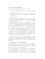
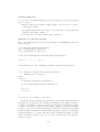
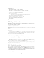
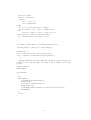
After the compilation, we get an executable file, mandel.seq, whose execution produces
the picture shown on the left side of 2.1.
2.3
Graphical execution
It is often useful to look at the structure of the application process network, for example
when tuning the performance of the final program. In OcamlP3l, this can be done by
compiling the program with the special option --graphical which automatically creates
a picture displaying the ‘logical’ parallel program structure.
ocamlp3lcc --graphical mandel.ml
26
Figure 2.1: A snapshot of the execution of mandel.ml (left is sequential execution,
right is parallel execution on 5 machines).
Remark 2.3.1 In the current implementation, this boils down to adding on top of mandel.ml
the line
open Grafp3l;;
to obtain a temporary file mandel.gra.ml which is then compiled via ocamlc with the
proper modules and libraries. Depending on the configuration of your system, this may
look like the following
ocamlc -custom graphics.cma grafp3l.cmo -o mandel.gra mandel.gra.ml
-cclib -lgraphics -cclib -L/usr/X11R6/lib -cclib -lX11
Once more, we highly recommend not to use explicit calls to ocamlc: use the ocamlp3lcc
compiler that is especially devoted to the compilation of OcamlP3lprograms.
¦
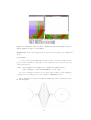
After compilation, we get the executable file mandel.gra, whose execution produces
the following picture.
27
2.4
Parallel execution
Once we have checked the sequential version of our code, and got a picture of the structure
of the parallel network, we are ready to speed up the computation by using a network of
computers.
2.4.1
Compilation for parallel execution
We call the compiler with the special option --parallel devoted to compilation for parallel
execution:
ocamlp3lcc --parallel mandel
Remark 2.4.1 In the current implementation this boils down to adding on top of mandel.ml
the lines
open Parp3l;;
open Nodecode;;
open Template;;
to obtain a temporary file mandel.par.ml which is then compiled via ocamlc with the
proper modules and libraries. Depending on the configuration of your system, this may
look like the following
ocamlc -custom unix.cma p3lpar.cma -o mandel.par mandel.par.ml
-cclib -lunix -cclib -lgraphics -cclib -L/usr/X11R6/lib
-cclib -lX11
Once again, we highly recommend not to use explicit calls to ocamlc: use the ocamlp3lcc
compiler that is especially devoted to the compilation of OcamlP3lprograms.
¦
The compilation produces an executable file named mandel.par.
2.5
Common options
The parallel compilation of OcamlP3l programs creates executables that are equipped with
the following set of predefined options:
• -p3lroot, to declare this invocation of the program as the root node.
• -dynport, to force this node to use a dynamic port number instead of the default
p3lport; in addition the option outputs it (useful if you want to run more slave
copies on the same machine).
• -debug, to enable debugging for this node at level n. Currently all levels are equal.
• -ip, to force the usage of a specified ip address. Useful when you are on a laptop
named localhost and you want to be able to choose among network interfaces.
• -strict, to specify a strict mapping between physical and virtual processors.
• -version, to print version information.
• -help or --help Displays this list of options.
28
2.5.1
Parallel computation overview
The executable produced by using the --parallel option of the compiler behaves either
as a generic computation node, or as the unique root configuration node, according to the
set of arguments provided at launch time.
To set up and launch the parallel computation network, we need to run multiple
invocations of the parallel executable:
• run one copy instance of mandel.par, with no arguments, on each machine that takes
part to the parallel computation; These processes wait for configuration information
sent by the designated root node,
• create a root node, by launching one extra copy of mandel.par with the special
option -p3lroot.
As soon as created, the root node configures all other participating nodes and then executes
locally the pardo encapsulated sequential code.
In addition to the -p3lroot special option, the root node invocation must specify
the information concerning the machines involved in the computational network (their ip
address or name, their port and color).
2.6
Launching the parallel computation
Here is a simple script to launch the parallel network on several machines:
#!/bin/sh
# The list of machines
NODES="machine1 machine2 machine3 machine4"
# The name of executable to be launched
PAR="./mandel.par"
echo -n "Launching OcamlP3L $PAR on the cluster:"
for NODE in $NODES; do
#(*1*)
echo -n " $NODE"
#launching a generic computation node on each machine
ssh $NODE $PAR 1> log-$NODE 2> err-$NODE &
# a possible coloring of machines
case $NODE in
#(*2*)
machine1) COLORED_NODES="$COLOREDNODES $NODE#1";;
*) COLORED_NODES="$COLOREDNODES $NODE#2";;
esac
done
echo "Starting computation with $COUNT node(s): $COLORED_NODES..."
# launch the unique root configuration node #(*3*)
$PAR -p3lroot $COLOREDNODES 1> log-root 2> err-root
echo "Finished."
This script assumes mandel.par to be accessible to all participating machines and does
the following:
29
• runs mandel.par on all participating machines (#(*1*)),
• generates a coloring for participating nodes (#(*2*)),
• launches the computation starting the root process on the local machine (#(*3*))
providing the list of colored participating hosts.
In future versions, especially those incorporating the MPI communication layer, the
startup mechanism will possibly work differently (typically, the initialization steps will be
performed by the MPI layer).
2.7
Common errors
A few words of warning now: even if the user program is now easy to write, compile and
execute, you should not forget that the underlying machinery is quite sophisticated, and
that in some situations you may not get what you expected. Two typical problems you
may encounter are the following:
output value: code mismatch If you see this error in the parallel execution of your
program, it means that two incompatible versions of your program are trying to
communicate. Ocaml uses an MD5 check of the code area before sending closures over
a channel, because this operation only makes sense between “identical” programs.
Two possible reasons for the error are:
• an old version of your program is still running somewhere and is trying to
communicate with the newer version you are running now. You should kill all
the running processes and try again.
• you are running copies of the program compiled for different architectures. This
feature is not yet supported, and you should run the program on homogeneous
architectures.
references You should remember that the user functions provided to the skeletons will be
all executed on different machines, so their behaviour must not rely on the existence
of implicitly shared data, like global references: if you do, the sequential behaviour
and the parallel one will be different. This does not imply that all user function
be real functions (you can use local store to keep a counter for example), but an
access to a global reference is certainly a mistake (since every node will access its
own private copy of the data, thus defeating the purpose of the shared data).
30
Chapter 3
More programming examples
3.1
Generating and consuming streams
Streams to be feed to the parallel networks can be created and consumed using functions
in P3lstream. Main functions are as follows:
Function
P3lstream.of list
Description
transforms a list in a valid stream
P3lstream.iter
iterates on all elements of a stream
P3lstream.of fun
allows stream generation
iterating a sequential function
which explicitely raises End_Of_File
transforms streams into lists
P3lstream.to list
3.1.1
Secs
3.1.1, 3.1.2,
3.5
3.1.1, 3.1.2,
3.1.3
3.1.3
3.1.4
Generating streams from lists
let rec generate_list_of_float n s =
if ( n <= 0 ) then []
else s :: (generate_list_of_float (n-1) (s +. 1.0))
;;
let initseq n s = P3lstream.of_list (generate_list_of_float n s);;
let finseq y =
P3lstream.iter (fun x -> print_float x; print_newline()) y;;
(* Define stage1 and stage 2, can be anything......*)
let stage1 _ x = x +. x;;
let stage2 _ x = x *. x;;
(* definizione network del pipe *)
let pipe = parfun (fun () -> seq(stage1) ||| seq(stage2));;
31
(* pardo activation *)
pardo
(fun () ->
let s = initseq 10 1.0 in
let y = pipe s in
finseq y
);;
3.1.2
Generating streams from files
let read_input_float fd =
Scanf.fscanf fd "%f" (fun n -> n);;
let rec fgenerate_list_of_float cin n=
if ( n <= 0 ) then []
else
(try
(let s = (read_input_float cin) in
Printf.printf "Ecco %f\n" s;
s:: (fgenerate_list_of_float cin (n-1)))
with
End_of_file -> [];
)
;;
(* stream generation *)
let initseq cin n =
P3lstream.of_list (fgenerate_list_of_float cin n);;
(* prints out stream *)
let finseq cout y =
P3lstream.iter (fun x -> Printf.fprintf cout "%f" x; output_string cout "\n") y;;
(* Defines stage1 and stage 2 *)
let stage1 _ x = x +. x;;
let stage2 _ x = x *. x;;
(* defining a two stage pipe network *)
let pipe = parfun (fun () -> seq(stage1) ||| seq(stage2));;
(* pardo activation *)
pardo
(fun () ->
let cin = open_in "pippo" and cout = open_out "pluto" in
let s = initseq cin 10 in
let y = pipe s in
finseq cout y
32
)
;;
3.1.3
Generating streams repeatedly calling a function
Here, the stream is generated by repeatedly calling function generate input stream via
P3lstream.of_fun.
%quinto-esempioUM.ml
(* generating the input stream calling repetedly a function *)
let generate_input_stream =
let x = ref 0.0 in
(function () ->
begin
x := !x +. 1.0;
if(!x < 10.0) then !x else raise End_of_file
end);;
(* prints out an integer stream *)
let finseq y =
P3lstream.iter (fun x -> print_float x; print_newline()) y;;
(* Defines stage1 and stage 2 as identity*)
let stage1 _ x = x;;
let stage2 _ x = x;;
let pipe = parfun (fun () -> seq(stage1) ||| seq(stage2));;
(* pardo activation *)
pardo
(fun () ->
let s = P3lstream.of_fun generate_input_stream in
let y = pipe s in
finseq y
)
;;
3.1.4
Transforming streams into lists
(* generating the input stream calling repeatedly a function *)
let generate_input_stream =
let x = ref 0.0 in
(function () ->
begin
x := !x +. 1.0;
if(!x < 10.0) then !x else raise End_of_file
end);;
(* Defines stage1 and stage 2*)
33
let stage1 _ x = x +. 1.;;
let stage2 _ x = x +. 7.;;
let print_result x =
print_float x; print_newline();;
let pipe = parfun (fun () -> seq(stage1) ||| seq(stage2));;
(* pardo activation *)
pardo
(fun () ->
let is = P3lstream.of_fun generate_input_stream in
(* transforms a stream into a list *)
let l = P3lstream.to_list (pipe is) in
List.iter print_result (List.map (fun n -> n*. 4.) l)
)
;;
3.2
Global and local definitions
As discussed in Section2.7, global variables must not be used in an OcamlP3l pragram, as
their value on different processing nodes will be different and updates will have effect only
on the node which executes them.
On the other hand, we can have both local and global definitions which are evaluated
before or after specializing a procesing node. For instance we can share the same file
descriptor between all the processing nodes partecipating to a skeleton. See examples in
Section 1.3.3.
3.3
Managing command line: option
To be done
3.4
Directing allocation: colors
To be done
3.5
Mixing Unix processes with OcamlP3l
The following code defines a farm in which each worker computes the square over a stream
of float. However, the function is computed by an external command which is spawned
and connected via stdin / stdout to the farm worker in the seq skeleton. In the following
code, care is taken to activate the external process only once. spawned is true only if the
Unix process and connecting pipes descriptor are maintained in variables cin and cout.
Notice that pattern matching in (* * *) is not exhaustive, because if process has been
already spawned cin and cout must contain a valid descriptor.
let farm_worker _ =
let conto = ref 0 and spawned = ref false
34
and cin = ref None
and cout = ref None in
(fun x ->
conto := !conto + 1;
if not !spawned then
begin
let (ic,oc) = Unix.open_process "./square"
in cin := Some ic; cout := Some oc; spawned:=true
end;
let Some ic, Some oc = (!cin , !cout) in (* * *)
Printf.fprintf oc "%d\n" x; Pervasives.flush oc;
let i = Scanf.fscanf ic "%d" (fun x -> x) in
)
;;
let compute = parfun (fun () -> farm(seq(farm_worker),4));;
let print_result x = print_int x; print_newline();;
pardo(fun () ->
let is = P3lstream.of_list [1;2;3;4;5;6;7;8;9] in
let s’ = compute is in P3lstream.iter print_result s’;
);;
The important thing is remember to fflush data output in the external commend source
otherwise we block. The following is an example of valid C definition for the square
program.
#include <stdio.h>
#define TRUE 1
int main(void)
{
int i;
while (TRUE) {
/* reading from standard input */
scanf("%d",&i);
/* writing on strandard output */
printf("%d\n",i*i);
/* fflushing buffers otherwise you block the output stream */
fflush(NULL);
}
exit(0);
}
35
Chapter 4
Implementing OcamlP3l
Now, let us point out the peculiar features relative to the implementation of OcamlP3l.
First, we will discuss the mechanism used to implement different processes onto different
nodes, by exploiting a particular form of “closure communication”. Then, we will point
out some details relative to the interprocess communication layer and we will motivate the
choice of the Unix sockets as the OcamlP3l communication layer. Finally, we will discuss
some details of the templates we used to implement the skeletons provided by OcamlP3l.
4.1
Closure passing as distributed higher order parameterization
A sequential implementation of an OcamlP3l program is quite easy to provide: just use a
library seqp3l.ml which implements each skelton with a valid Ocaml sequential function.
The type safety is a direct consequence of the fact that we are not using here anything
from outside the safe core of Ocaml.
Similarly, providing the graphical semantics poses no real challenge.
But what about the parallel semantics? What is the right way to implement such
a thing? We must guarantee the type safety and ensure that the runtime is reasonably
small as to allow the verification of its properties, which will become an important point
in industrial applications. Both points posed problems which we overcame during the
development of the system.
First of all, to ensure that the system is manageable and safe, we immediately discarded
the approach based on parsing the source file to extract the code corresponding to each
node of the network: this would impose to use external tools to perform an analysis of the
user code which is difficult, error prone, and whose semantics would have a very unclear
status.
Instead, we choose to use an SPMD approach: all the nodes of the network will run
the same program (in a sense this is the “template process interpreter code”, as we will see
in while) , which will be the result of the compilation of the full user code, and a control
node1 will dispatch to the rest of the nodes in the network the parameterization information
needed to specialize it to the particular function it is really supposed to perform (emitter,
collector, sequential node running a given function f , etc.).
1 The
control node runs the same program as the others, but it is invoked by the user with a
special designating option -p3lroot.
36
In order to achieve this behavior, the control node performs the following tasks:
• executes the parfun skeleton expression definitions, which has as a consequence to
build a data structure describing all the parallel process networks. From this data
structure, we compute behind the scenes the configuration information for each node
in the process network.
• executes the pardo expression: this has the following effect
– maps virtual nodes to the processor pool given on the command line,
– initializes a socket connection with all the participating nodes,
– gets the port addresses from each of them (a fixed port number —p3lport—
or some dynamically generated number if more than one copy run on the same
machine),
– sends out to each node the addresses of its connected neighbors (this step
together with the previous two provides an implementation of a centralized
deadlock free algorithm to interconnect the other nodes into the process network specified by the skeleton expression),
– sends out to each node the specialization information that consists of the function it must perform.
This very last task requires a sophisticated operation: sending a function (or a closure)
over a communication channel. This is usually not possible in traditional functional programming languages, since sending an arbitrary function supposes that we are able to find
on the receiving side the code corresponding to the function name received or that we can
transfer executable code (a feature known as mobility today). Now, mobility is necessary
to send closures between arbitrary programs (since two different programs have no reason
to know each other’s function code), but not between two copies of the same program:
in the latter case, it suffices to send what essentially amounts to a code pointer. Starting
from version 1.06, Ocaml contains a modified marshaling library, originary designed for
the OcamlP3l system, that performs closure sending between copies of the same program
(this is checked by means of an MD5 signature of the program code). The ocaml run
time system takes care of dealing with differences in endianness and word size between
communicating machines, as well as flattening tree-shaped data structures.
On the other side, all the other nodes simply wait for a connection to come in from the
root node, then send out the address of the port they allocate to do further communication,
wait for the list of neighbors and for the specialization function, then simply perform it
until termination.
To summarize, in the implementation the possibility of sending closures allowed us to
obtain a kind of higher order distributed parameterization that kept the runtime code to
a minimum size (the source codes of the full system is less than twenty kilobytes).
4.2
Communication and process support
As far as the general mechanism of closure passing is concerned, no particular requirement/restrictions have been posed onto the physical communication implementation. Even
considering the fact that we need to move data between the different processes making up
the parallel implementation of an OcamlP3l program, we derived no particular constraint
onto the communication layer.
37
Thus, at the very beginning of the OcamlP3l project, we faced the problem of choosing
a suitable communication system. We had as a goal to come out with the maximum
“portability” of OcamlP3l. Furthermore, we wanted to fully demonstrate the feasibility
of integrating the parallel skeleton world within a functional framework. These two goals
had priority over the classical “efficiency and performance” goal one usually has to achieve
when dealing with parallelism.
The result is that we have adopted the plain Unix socket world as the communication
layer. This has some (very) positive consequences on the overall OcamlP3l design:
• the socket communication support is generally available on Unix/Linux and Windows system
• no particular customization of the support is needed to match the OcamlP3l features,
• the point-to-point, connection oriented, stream model provided by Unix sockets is
perfect to model data streams flowing around between the processes belonging to
the process network derived by OcamlP3l to implement the user skeleton code,
• last but not least, there was an existing and suitable ocaml interface to Unix system
calls, including those relative to sockets.
On the down side, the adoption of Unix sockets presents an evident disadvantage which
is the low performance achieved in communications (a raw synchronization (i.e. zero length
data communication) takes several milliseconds to be performed, even in those cases when
the data transmission media turns out to be free, i.e. no collisions are detected).
At the moment, we are considering to use in the next version of OcamlP3l a communication layer based on an optimized communication library such as MPI [18], as an efficient
alternative to the socket communication layer, which will be nevertheless retained for its
ease of deployment, that makes it attractive for programming courses.
Porting to MPI will require some modifications in the template code used within
OcamlP3l, and will not necessarily completely solve the performance problems of the socket
communication layer when run on a network of computers, where most MPI libraries are
still implemented using sockets, but will allow to target real multiprocessor machines where
MPI is efficiently implemented, without touching the user code. Also, we will be able to
delegate to the MPI system the administrative tasks involved in copying and launching
the programs on the different machines.
As far as the process model is concerned, we felt happy with the Unix one. All we need
is a mechanism allowing an instance of the template interpreter (the one specialized by
using the closure passing mechanism) to be run onto different workstations belonging to
a local area network. The Unix rsh mechanism matches this requirement. Note that, as
processes are generated and run on different machines just at the beginning of the OcamlP3l
program execution, any considerations about performance in rsh-ing is irrelevant.
4.3
Template implementation
OcamlP3l implements each skeleton appearing in the application code by generating a
proper instantiation of the corresponding implementation template. In OcamlP3l, a single
implementation template is provided for each one of the skeletons supported. The implementation templates provided within the current prototype closely resemble the ones
discussed in the informal parallel semantics section (Section 1.3). Actually, only the reduce template is slightly different, in that the tree discussed in Section 1.3.7 is actually
38
implemented by a process network similar to the one discussed for the farm, where partially evaluated data is iteratively passed back from the collector to the emitter process.
We are currently studying a more efficient mechanism based on a formal calculus for data
distribution and computation over dense arrays [17, 8, 7].
Each template appearing in OcamlP3l:
• is parametric in the parallelism degree exploited As an example the farm template
may accommodate any positive numbers of worker processes. Currently, the programmer must specify this parameter, which is the second parameter of a farm(f,n)
skeleton call.
• is parametric in the function computed as the body of the skeleton For instance,
the farm skeleton accepts as a parameter the function that has to be computed by
the worker processes. This function must be a skeleton itself. Therefore, either it
is a seq skeleton call, or it is a skeleton call modeling a parallel computation. In
the former case, the skeleton is implemented by a process network whose workers
just perform the sequential computation f denoted by some seq(f). In the latter
case, each worker process is itself a process network known by the emitter and
collector processes implementing the farm just as channels where data has to be
delivered/fetched.
• provides a set of process templates i.e. parametric process specifications that can be
instantiated to get the real process codes building out the implementation template
process network. As an example, consider again the farm template. The emitter
process behavior can be fully specified by the data type of items that have to be
processed, by the channel from which those data items have to be read and by the set
of channels onto which the data items have to be scheduled (written) to the worker
processes, possibly with some “clever” (e.g. achieving load balancing) scheduling
strategy. Such a process can be completely specified by providing a function
farmetempl (OutChanSel f) ic ocl
whose first parameter provides the worker scheduling function, the second one provides the input channel where data has to be fetched and the third one provides the
set of channels used to deliver tasks to be computed to the farm workers. The type
of such a function turns out to be
val farmetempl : (’a, ’b) Parp3l.action -> in_channel ->
out_channel list -> unit
The process template definition in the OcamlP3l code looks like the following:
let farmetempl (OutChanSel f) ic ocl =
while true do
try
let theoc = f ocl in
match (Marshal.from_channel ic) with
UserPacket(p,seqn,tl) ->
Marshal.to_channel
theoc
(UserPacket (p,seqn,Farmtag::tl))
[Marshal.Closures];
flush theoc;
| EndStream ->
39
List.iter
(fun x -> Marshal.to_channel
x
EndStream
[Marshal.Closures];
flush x)
ocl;
List.iter close_out ocl; close_in ic; exit 0
with End_of_file -> List.iter close_out ocl;
close_in ic
done;;
Therefore the whole compilation process transforming an OcamlP3l skeleton program into
the parallel process network implementing the program can be summarized in the following
steps:
1. the skeleton code is parsed and transformed into a skeleton tree data structure,
recording all the significant details of the skeleton nesting supplied by the user code,
2. the skeleton tree is traversed and processes are assigned to each skeleton according
to the implementation templates. During this phase, processes are denoted by their
input/output channels, identified via a unique number.
3. once the number and the kind of parallel processes building out the skeleton code
implementation is known, code is generated that either delivers the proper closures,
derived by using the process templates, to the “template interpreter” instances running on distinct workstations (this happens just on one node, the “root” one), or
waits for a closure and repeatedly computes this closure on the proper input and
output channels until an EndOfFile mark is received.
40
Chapter 5
Multivariant semantics and
logical debugging
By providing modules that implement the three OcamlP3l skeleton semantics (the sequential one, the parallel one and the graphical one), we allow the OcamlP3l user to perform
the following parallel application development process:
• develop skeleton code modeling the application at hand. This just requires a full
understanding of the skeleton sequential semantics and usually allows the user to
reuse consistent portions of existing applications written in plain ocaml or legacy in
C, C++ etc.
• test the functionality of the new application by supplying relevant input data items
and looking at the results computed using the sequential skeleton semantics. In case
of problems, the user may run the sequential debugging tools to overcome problems.
• link the parallel skeleton semantics module and run the application onto the workstation network. Provided that the application was sequentially correct, no new
errors should be found at this step (we assume that the run time is guaranteed correct!). In practice, a few errors can occur ussually related to wrong assumption on
global variables. If your code uses global variables updating them durin gexecution,
this will work OK in the sequential semantics as memory is actually shared but not
in the parallel version as update will be only seen locally on the processing node.
• look at the performance results of running the application on the number of processors available and possibly adjust the significant performance parameters, such as
the number of workers of the farm, map and reduce and the color of each of them.
This is actually the real problem in the development of an efficient parallel application. Forthcoming versions of OcamlP3l will include analytical performance models
for the templates and these models will be used to automatically guess colors and
giude the complier in the compiler. During performance tuning, the programmer
may link the graphic semantic skeleton module and look at the results of the program execution, i.e. at the resulting process graph, in order to understand where
bottlenecks are or which parts of the program must be further decomposed using
skeletons in order to get better performant application code.
Let us spend now some words concerning logical, sequential debugging of OcamlP3l
applications.
41
A user developing an OcamlP3l application may link the sequential skeleton semantics
module to his/her code and debug the application by using the plain sequential debugging
tools of ocaml. This debugging activity can be performed on a single machine, provided
the machine supplies ocaml. Also, performance tuning can be directed using standard
sequential profiling tools such as gprof.
Once the application has been debugged, i.e. the user perceives it computes the expected results, he/she can compile the parallel version of the application by linking the
parallel skeleton semantics. As we guarantee that the implementation templates for the
different skeletons of OcamlP3l are correct (deadlock free, load-balanced, etc.) and as we
guarantee that the process transforming the skeleton code in the process code is correct,
the user does not need to perform explicit activities in order to check that the results
computed by the parallel code are correct.
In particular, the user does not need to check that all the processes have been correctly
scheduled for execution, or that the communication channels have been set up properly
between these processes, or that data of type ’a has been never delivered on channels
transmitting data of type ’b. This is a very short list of bad things that may affect the
correct behavior of an explicitly parallel program, indeed. The fact that the user is not
required at all to take them into account is one of the biggest pro’s of the functional
skeleton approach.
42
Chapter 6
Related work, conclusions
and perspectives
6.1
Related work
Many researchers are currently working on skeletons and most of them are building some
kind of parallel implementation, but our work, as far as we know, is unique in its combination of a fully functional strongly typed language with the skeleton approach.
In particular, Darlington’s group at Imperial College in London is actively working on
skeletons. They have explored the problems relative to implementing a skeleton programming system, but the approach taken uses an imperative language as the implementation
language. Currently there is a “local” prototype implementation but no public domain
implementation of their skeleton approach and they seem deeply involved in the study of
the data-parallel and coordination aspects of skeletons. [13, 12, 1]
A different approach relative to skeleton parallel programming within a functional
framework has been discussed by Bratvold [4]. Bratvold takes into account plain ML
programs and looks for skeletons within them, compiling these skeletons by using process
networks that look like implementation templates. However, both the final target language
and the implementation language are imperative.
Finally, Sérot [23, 22], presents an embedding of skeletons within ocaml that seems to
be close to our work, although independently developed. The message passing is performed
by interfacing the MPI library with ocaml. The skeletons taken into account are different.
She considers data-parallel farm, roughly corresponding to our mapvector skeleton, and
two further skeletons, scm and filt. filt is a plain filter skeleton, canceling data items
from a list, while scm (Split, Compute and Merge) looks like a map skeleton working on
lists with explicit, user defined, decomposition/recomposition functions.
Sérot’s implementation of the skeletons within ocaml is quite different from ours and
only allows one skeleton at a time to be realized on the processor networks, thus preventing
skeleton composition (you cannot nest two scm skeletons for example), and only allowing
for a limited form of staging of the parallel computation: you can perform an scm, then
when this is finished, you can reorganize your network and perform another scm. This
way, the mapping of virtual processors to real processors on the network is a trivial task,
and is done inside each skeleton at run-time instead of beforehand in a specific pass like
in OcamlP3l. Sérot implements the skeletons included in his model by providing second
43
order functions that directly call MPI and realize an SPMD execution model.
As for the relevant effort done in the field of languages for mobile agents, like for
example [16, 15], it should be noted that they address quite a different kind of problems,
but once stable, these languages could form the basis of a next generation fully faulttolerant and dynamically load-balanced version of our system.
6.2
Conclusions and perspectives
Here we showed how a skeleton parallel programming modelcan be successfully married
with the functional programming environments such as the one provided by Ocaml.
In particular, we discussed a powerful skeletal model, how skeletons can be embedded
within Ocaml as second order functions and how modules implementing both the sequential
and the parallel skeleton and discuss the typical application development cycle in OcamlP3l.
The whole process preserves the strong typing properties of ocaml.
At the moment, the prototype OcamlP3l implementation is being tested as described
in this paper and is available from the OcamlP3l project home Web page
http://www.dicosmo.org/ocamlp3l/.
In the near future we want first of all to include a more powerful MAP skeleton working
on dense arrays with an arbitrary number of dimensions[17, 8, 7]. This will call for a more
efficient communication layer, by using colective MPI communications [18] instead of the
plainUnix socket library. At the same time, we investigate the feasibility of porting the
system on the ubiquitous Windows boxes, for didactical purposes. Finally, we already
developed a parallel numerical code [5] and plan to write some more significant parallel
applications in order to fully test the prototype.
44
Bibliography
[1] P. Au, J. Darlington, M. Ghanem, Y. Guo, H.W. To, and J. Yang. Co-ordinating
heterogeneous parallel computation. In L. Bouge, P. Fraigniaud, A. Mignotte, and
Y. Robert, editors, Europar ’96, pages 601–614. Springer-Verlag, 1996.
[2] B. Bacci, M. Danelutto, S. Orlando, S. Pelagatti, and M. Vanneschi. P3 L: A Structured High level programming language and its structured support. Concurrency
Practice and Experience, 7(3):225–255, May 1995.
[3] R. S. Bird. An introduction to the Theory of Lists. In M. Broy, editor, Logic of
programming and calculi of discrete design, volume F36 of NATO ASI, pages 5–42.
Springer-Verlag, Berlin, 1987.
[4] T. Bratvold. Skeleton-Based Parallelisation of Functional Programs. PhD thesis,
Heriot-Watt University, 1994.
[5] François Clément, Roberto Di Cosmo, Zheng Li, Vincent Martin, Arnaud Vodicka,
and Pierre Weis. Parallel programming with the system applications to numerical
code coupling. Technical Report RR-5131, INRIA Roquencourt, 2004.
[6] M. Cole. Algorithmic Skeletons: Structured Management of Parallel Computations.
Research Monographs in Parallel and Distributed Computing. Pitman, 1989.
[7] Roberto Di Cosmo, Zheng Li, and Susanna Pelagatti. A calculus for parallel computations over multidimensional dense arrays. to appear on Computer Languages,
Systems and Structures special issue on “Semantics and Cost models for High-Level
Parallel Programming”, 2005.
[8] Roberto Di Cosmo and Susanna Pelagatti. A cost calculus for dense array distributions. Parallel Processing Letters, 13(3):377–388, 2003.
[9] M. Danelutto, R. Di Meglio, S. Orlando, S. Pelagatti, and M. Vanneschi. A methodology for the development and support of massively parallel programs. Future Generation Computer Systems, 8(1–3):205–220, July 1992.
[10] Marco Danelutto, Roberto Di Cosmo, Xavier Leroy, and Susanna Pelagatti. Parallel
functional programming with skeletons: the ocamlp3l experiment. The ML Workshop,
1998.
[11] J. Darlington, A. J. Field, P. G. Harrison, P. H. J. Kelly, D. W. N. Sharp, and
Q. Wu. Parallel Programming Using Skeleton Functions. In PARLE’93, pages 146–
160. Springer, 1993. LNCS No. 694.
[12] J. Darlington, Y. Guo, H. W. To, Q. Wu, J. Yang, and M. Kohler. Fortran-S: A
Uniform Functional Interface to Parallel Imperative Languages. In Third Parallel
Computing Workshop (PCW’94). Fujitsu Laboratories Ltd., November 1994.
45
[13] J. Darlington, Y. Guo, H. W. To, and J. Yang. Parallel Skeletons for Structured
Composition. In Fifth ACM SIGPLAN Symposium on Principles and Practice of
Parallel Programming. ACM Press, July 1995.
[14] Cédric Fournet and Georges Gonthier. The reflexive chemical abstract machine and
the join-calculus. In Proceedings of the 23rd ACM Symposium on Principles of Programming Languages, pages 372–385, St. Petersburg Beach, Florida, January 21-24
1996. ACM.
[15] Cedric Fournet and Luc Maranget. The Join-Calculus language. INRIA, June
1997. Software and documentation available electronically, (http://pauillac.inria.fr/join).
[16] F. C. Knabe. Language Support for Mobile Agents. PhD thesis, School of Computer Science, Carnegie Mellon University, 1995. CMU-CS-95-223; also published as
Technical Report ECRC-95-36.
[17] Zheng Li. Efficient implementation of MAP skeleton for the OcamlP3L system. DEA
Report, Université PARIS VII, July 2003.
[18] M.P.I.Forum. Document for a standard message-passing interface. Technical Report
CS-93-214, University of Tennessee, November 1993.
[19] S. Pelagatti. A methodology for the development and the support of massively parallel
programs. Technical Report TD-11/93, Dept. of Computer Science – Pisa, 1993. PhD
Thesis.
[20] S. Pelagatti. Structured development of parallel programs. Taylor&Francis, London,
1998.
[21] S. Pelagatti. Task and data parallelism in P3L. In Fethi A. Rabhi and Sergei Gorlatch,
editors, Patterns and Skeletons for Parallel and Distributed Computing, chapter 6,
pages 155–186. Springer-Verlag, London, 2002.
[22] J. Sérot and D. Ginhac. Skeletons for parallel image processing : an overview of the
SKiPPER project. Parallel Computing, 28(12):1785–1808, Dec 2002.
[23] Jocelyn Sérot. Embodying parallel functional skeletons: an experimental implementation on top of MPI. In Proceedings of the EuroPar 97. Springer Verlag, LNCS No.
1300, 1997. Passau, Germany.
46