Download Real-Time Software User`s Manual

Real-Time Software User’s Manual
SOAR Adaptive Module (SAM)
Revision 1.9, May 2011
Contents
Getting Things Running
1.1 Hardware Setup...............................................................................................................................1
1.2 Starting the Real-Time Software.....................................................................................................1
1.3 Stopping the Real-Time Software...................................................................................................2
1.4 Recovering from a VNC crush........................................................................................................2
GUI Reference
2.1 MAIN>Operation Tab.....................................................................................................................4
2.1.1 MAIN>Operation>AOLoop Window.....................................................................................6
MAIN>AOLoop>File Menu........................................................................................................6
MAIN>AOLoop>Tools Menu.....................................................................................................6
MAIN>AOLoop>Graphs Menu..................................................................................................7
MAIN>AOLoop>Loop Control Tab............................................................................................7
MAIN>AOLoop>Interaction Matrix Tab....................................................................................7
MAIN>AOLoop>Reconstructor Matrix Tab...............................................................................8
MAIN>AOLoop>Reconstruction Error Tab................................................................................8
2.1.2 MAIN>Operation>WFS Window...........................................................................................8
MAIN>WFS>File Menu..............................................................................................................8
MAIN>WFS>Tools Menu...........................................................................................................9
MAIN>WFS>Graphs Menu........................................................................................................9
MAIN>WFS>WFS Configuration Tab......................................................................................10
MAIN>WFS>Modal Estimation Tab.........................................................................................10
MAIN>WFS>Pockels Cell Tab.................................................................................................10
2.1.3 MAIN>Operation>WFS>Display Window...........................................................................10
2.1.4 MAIN>Operation>TTLoop Window....................................................................................11
MAIN>TTLoop>File Menu.......................................................................................................11
MAIN>TTLoop>Tools Menu....................................................................................................11
MAIN>TTLoop>Graphs Menu.................................................................................................12
MAIN>TTLoop>Loop Control Tab...........................................................................................12
2.1.5 MAIN>Operation>DM Window...........................................................................................12
MAIN>DM>Voltages Tab.........................................................................................................12
MAIN>DM>Graph Tab.............................................................................................................13
2.2 MAIN>Historical Tab...................................................................................................................13
2.3 MAIN>Maintenance Tab...............................................................................................................13
2.4 MAIN>Comm-Server Tab.............................................................................................................14
2.5 MAIN>Comm-Client Tab.............................................................................................................14
Common Operations
3.1 Calibrating the Wavefront Sensor..................................................................................................15
3.2 Obtaining the Reconstructor Matrix H*........................................................................................15
3.3 Saving AO Loop Data Sequences.................................................................................................16
3.4 Examining the AO Loop Performance..........................................................................................16
ii
3.5 Poking the DM Electrodes............................................................................................................17
Configuration Files and Macros
4.1 Configuration Files........................................................................................................................19
4.1.1 rtsoft.cfg – real-time software parameters.............................................................................20
4.1.2 camera.cfg – WFS CCD controller parameters.....................................................................20
4.1.3 flattendm.cfg – voltage values to make de DM flat...............................................................21
4.1.4 positions.ini – WFS geometry and reference spot positions..................................................21
4.1.5 positions_bgnd.ini – background subtraction box definitions...............................................21
4.1.6 zstatic.ini – static aberrations.................................................................................................22
4.1.7 zlabel.ini – zernike mode label file........................................................................................22
4.1.8 eltrdmap.ini – electrodes look up table..................................................................................22
4.1.9 apdmap.ini – APD look up table............................................................................................23
4.1.10 apdbias.ini – APD biases.....................................................................................................23
4.1.11 soar_comms.ini – SOAR communicaton library parameters..............................................23
4.1.12 faults.ini - faults definitions................................................................................................23
4.2 Macros...........................................................................................................................................24
4.3 FITS files.......................................................................................................................................26
4.3.1 bim.fits...................................................................................................................................26
4.3.2 cmat.fits – Noll covariance matrix.........................................................................................26
4.3.3 imat.fits..................................................................................................................................26
4.3.4 rmat.fits and nas_rmat.fits.....................................................................................................26
4.3.5 wfsbias.fits.............................................................................................................................26
4.3.6 mask.fits.................................................................................................................................27
badpix.fits...................................................................................................................................27
amps.fits.....................................................................................................................................27
4.3.7 weight.fits, xgrid.fits, ygrid.fits.............................................................................................27
Simulator Modes
5.1 Simulation at user space level.......................................................................................................29
5.2 Simulation at kernel space level....................................................................................................29
5.3 Simulation Parameters...................................................................................................................30
5.3.1 User defined pattern...............................................................................................................30
5.3.2 5.3.2 FITS file........................................................................................................................30
5.3.3 Zernike Modes.......................................................................................................................30
5.3.4 Kolmogorov...........................................................................................................................30
Log Files
6.1 Type Alarm Events........................................................................................................................31
Glossary
iii
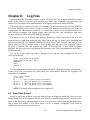
Chapter 1:Getting Things Running
Chapter 1:
Getting Things Running
This user manual is intended to describe the use of the Real-Time Software (RTSOFT) from a user's
point of view. It is not a programming manual. For implementation details please read the Real-Time
Software Programmer Manual (RTSPM).
1.1 Hardware Setup
Before firing up the RTSOFT, and with the real-time computer turned off, there is a list of hardware
that has to be powered up:
a) Turn on the CCD controller power supply. Real-Time computer should be turned off at this
time!
b) Turn on the Peltier cooler power supply.
c) Turn on the water pump.
d) Turn on the high voltage amplifier of the DM.
e) Turn on the PXI chassis. Real-Time computer should be turned off at this time!
IMPORTANT: The real-time computer should be turned off when powering up the CCD
controller and the PXI chassis. This assures correct detection of the devices by their interface
boards in the real-time computer.
1.2 Starting the Real-Time Software
Before you start the real-time software, make sure that all items in the checklist above were checked.
It is very important to check the above list in order for the boot process to succeed.
a) Turn on the real-time computer an wait for the system to boot.
b) Start a VNC session connected to the real-time computer or alternatively log on as user ao and
fire up the X windows system.
c) Press the SAM RTC button in the toolbar or alternatively open a shell window and invoke the
real-time software application with the following command:
% cd /home/ao/RTsoft
% labview RTsoft.vi -- [ options]
Normally, you will invoke RTSOFT with no options. Options are reserved in case part of the
hardware is not present and is wanted to be simulated by software. Valid option values are listed below:
-c
No camera controller hardware is present.
-d
No deformable mirror hardware is present.
-r
Real-Time Core module not installed.
1
Rtsoft User Manual Rev 1.9, May 2011
Chapter 1:Getting Things Running
-tcs
No connection to the TCS server
-lm
No connection to the Laser Module server.
1.3 Stopping the Real-Time Software
To stop the RTSOFT application click the EXIT button. A dialog box will prompt for confirmation.
Press YES.
1.4 Recovering from a VNC crush
If the VNC connection to the RTC is lost there are ways to recover:
1. Check first if it's only a VNC problem and not a system crush by pinging the machine.
2. If the machine is not responding, reboot the RTC and proceed as described in section 1.2 above.
3. If the machine is alive, ssh to the machine and type the following command to restart the VNC
server
% bin/startvnc
4. Proceed as described in section 1.2 above paragraph c.
Rtsoft User Manual Rev 1.9, May 2011
2
Chapter 2:GUI Reference
Chapter 2:
GUI Reference
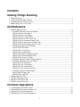
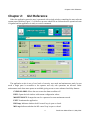
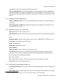
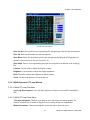
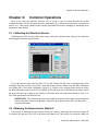
When the application starts the user is presented with a single window containing the most relevant
system status variables (Figure 2.1). If the boot process ended with no failures then the operational state
is signaled and the application is ready to receive commands.
Figure 2.1: Main GUI. The most relevant status variables are displayed.
The application works in one of two levels of security: user mode and maintenance mode. In user
mode a single pane is accessible to the operator and only safe operations are allowed. Under
maintenance mode three more panes are available giving access to more advanced and risky features.
CLEAR ALARM. Allows the user to turn the alarm condition off.
INFO. Opens the info window with current configuration values.
MAINTENANCE. Prompts the user for a password to enter maintenance mode.
EXIT. Terminates the application.
DM Loop. Indicates whether the AO control loop is open or closed.
M3 Loop. Indicates whether the M3 control loop is open or closed.
3
Rtsoft User Manual Rev 1.9, May 2011
Chapter 2:GUI Reference
Mount Loop. Indicates whether the Mount control loop is open or closed.
LLT Loop. Indicates whether the LLT loop is active or not. Available under LGS mode only.
TT Loop. Indicates whether the tip tilt loop is active or not. Available under LGS and NGS
modes.
Bias Subtraction. Indicates that frame bias subtraction is active.
Simulator Mode. Indicates whether a simulator mode is active or not. See section 5 below for
details on how the simulator modes work.
Operation Mode. Indicates what operation mode is active: TURSIM, NGS, TSLGS or LGS.
r0 [m]. Seeing estimate.
Wind [m/s]. Wind speed estimate.
VAR C.M.[rad2]. Variance of the corrected modes in [rad2].
AO Loop [ms]. Average AO loop period.
WFS Flux [Ke-/s]. Wavefront sensor stellar flux in Kilo-photons per second per sub-aperture
TT Loop [ms]. Average TT loop period in [ms].
GP1 Flux [Ke-/s]. Guide probe 1 stellar flux in Kilo-photons per second.
GP2 Flux [Ke-/s]. Guide probe 2 stellar flux in Kilo-photons per second.
2.1 MAIN>Operation Tab
The operation tab is the only pane that the operator will use under normal operation. Four lowered
rounded boxes group the controls and indicators by functionality.
AO Loop... Opens the AO Loop Control Window. Read section 2.1.1 below.
DM Loop. Open/Close the DM control loop.
Operation Mode. List box to select the current operation mode:
TSNGS. TurSim natural guide star mode.
NGS. Natural guide star mode.
TSLGS. TurSim laser guide star mode
LGS. Laser guide star mode.
WFS... Opens the WFS Control and WFS Display windows. Read sections 2.1.2 and 2.1.3
below.
TT Loop... Opens the TT Loop Control Window. Read section 2.1.4 below.
M3 Loop. Open/Close the M3 control loop.
Mount Loop. Open/Close the Mount control loop.
LLT Loop. Open/Close the LLT control loop.
Rtsoft User Manual Rev 1.9, May 2011
4
2.1
2.1.1
RTS MAIN
GUI
AOLoop
File
2.1.1.1
2.1.1.2
Tools
Load/Save I.Mat
Load/Save
R.Mat.
●Save Loop Data
2.1.1.3
Graphs
●
●
●
●
Rec.Error
AO Loop
Perf.
Modal
Coefs.
●Noise Prop.
●
●
●
●
Maintenance
2.1.1.4
2.2
Historical
Comm-Server
Comm-Client
2.1.1.5
Loop Control
2.3
2.1.1.6
Interaction
Matrix
Reconstructor
Matrix
Open/Close
Control Law
●
2.4
●
2.5
2.1.2
WFS
File
2.1.2.1
Load/Save
Ref
●Save G/G*
●Save Frames
●Load Bias
●
Tools
2.1.2.2
2.1.2.3
Graphs
Flux &
FWHM
●Slopes
●Histogram
DSP Commands
●Bias Calibration
●Mask
●Weight Template
●C.C. Template
●Static Aberrations
●
●
2.1.2.4
WFS
Configuration
Exposure Time
Bias On/Off
2.1.2.5
Modal
Estimation
Zernike Coefs.
Set Regerences
●
●
●
●
2.1.3
WFS
Display
2.1.4
TTLoop
File
2.1.4.1
Save Loop
Data
●
Tools
2.1.4.2
Graphs
2.1.4.3
Flux
●Centroids
Mount
●LLT
●
●
2.1.4.4
Loop Control
Time Base
●
2.1.5
DM
2.1.5.1
Graphs
Voltages
2.1.5.2
Load/Save
Table
●
●
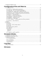
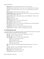
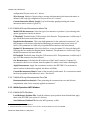
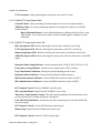
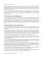
Figure 2.2: User Interface Navigation Map
2.1.4.5
Response
Chapter 2:GUI Reference
DM... Opens the DM Window. Read section 2.1.5 below.
STATIC FLAT. Loads and applies the voltages stored in the file flattendm.cfg to the DM.
ROT FLAT. Loads and applies the voltages stored in the file flattendm.cfg including a
correction factor based on the current rotator angle.
2.1.1 MAIN>Operation>AOLoop Window
2.1.1.1 MAIN>AOLoop>File Menu
Load Interaction Matrix. Allows for loading a previously saved interaction matrix. The matrix
to load is expected to be in standard FITS file format.
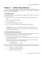
Figure 2.3: Loop Control GUI. This window is used to obtain reconstructor
matrix.
Save Interaction Matrix. Allows for saving the current interaction matrix. The matrix is saved
in standard FITS file format as imat.fits and imat-<current date>.fits
Load Reconstructor Matrix. Load FITS file containing reconstructor matrix definition. The
matrix is loaded into memory only.
Save Reconstructor Matrix. Save the current reconstructor matrix to disk in FITS file format
in the RTsoft/ConfigFiles/ directory.
Save Loop Data Sequence. Save real-time sequences of slopes and voltages to disk. Read
section 3.3 below.
2.1.1.2 MAIN>AOLoop>Tools Menu
Reconstruction Error Analysis. Chart presenting the reconstruction error and effective
Rtsoft User Manual Rev 1.9, May 2011
6
Chapter 2:GUI Reference
compensation order for the currently applied reconstructor1.
AO Loop Performance. Window presenting the user with atmospheric and loop performance
estimates and graphs. This window is intended to be used as diagnostic tool to study AO loop
compensation of the atmospheric disturbances. Read section 3.4 for more details on how to use
this tool.
2.1.1.3 MAIN>AOLoop>Graphs Menu
Modal Coefficients Charts. Set of charts presenting real-time sequences of slopes and modal
coefficients.
Noise Propagation Coefficients. Graph presenting the noise propagation coefficients for the
current reconstructor matrix.
2.1.1.4 MAIN>AOLoop>Loop Control Tab
AO Loop. Open close the AO loop control.
Tilt Subtraction. Indicator showing if tilt component subtraction from residual measurements
is
active.
Operation Mode. Indicates what operation mode is active: TURSIM, NGS, TSNGS or LGS.
Loop Time. Average AO loop period in [ms].
r0 [m]. Seeing estimate.
Wind [m/s]. Wind speed estimate.
Time Constant.
VAR C.M.[rad2]. Variance of the corrected modes in rad2.
Control Law. Allows the user to select between Smith predictor and pure integrator as the
control law for the AO loop. Depending on selection the right parameter values are shown.
K. Pure integrator and Smith predictor gain.
KL. Leaky constant.
KS. Smith predictor constant. Visible only when SP control law has been selected.
AO Loop. Open/Close the DM control loop.
2.1.1.5 MAIN>AOLoop>Interaction Matrix Tab
Get Interaction Matrix. Pops up the “Interaction Matrix Measurement” window. Read section
3.2 below.
Mid Voltage [V]. Mid range voltage value. This value is typically 0 as defined in the rtsoft.cfg
1
Detailed information on this analysis can be found in document SDN1107 and in the RTSPM.
7
Rtsoft User Manual Rev 1.9, May 2011
Chapter 2:GUI Reference
configuration file (see section 4.1.1 below).
SD to Average. Number of slope values to average when measuring the interaction matrix as
defined in the rtsoft.cfg configuration file (see section 4.1.1 below).
Current Interaction Matrix Graph. Gray level intensity graph presenting the current
interaction matrix in units of [pixel/V].
2.1.1.6 MAIN>AOLoop>Reconstructor Matrix Tab
Modal/SVD Reconstructor. Select the type of reconstructor to produce. Upon selecting each
option, appropriate controls are shown.
P Threshold. Threshold in the SVD inversion of the P matrix. This parameters is visible only if
type Modal Reconstructor has been selected.
Regularization Parameter. This is the alpha parameter for the optimized reconstructor2. Set
this parameter to the desired value before obtaining a reconstructor matrix (see section 3.2
below). This parameters is visible only if type Modal Reconstructor has been selected.
Optimal G* Reconstructor. Select this check box to use the optimal G* when calculating H*.
Selecting this box enables the Regularization Parameter. This parameters is visible only if type
Modal Reconstructor has been selected.
H Threshold. Threshold when doing the SVD inversion of H. This parameters is visible only if
type SVD Reconstructor has been selected.
Get Reconstructor. Calculates the H* matrix out of the P and G matrices. If optimal G*
reconstructor check box is selected, then the optimal G* matrix is used when obtaining H*.
Apply Reconstructor. Apply the reconstructor matrix to the RTCORE. If a reconstructor
matrix has been loaded and not applied, this button will blink.
Current Reconstructor Matrix. Name of the currently loaded matrix. If a reconstructor matrix
has been just produced the indicator is set to “Not Saved”.
2.1.1.7 MAIN>AOLoop>Reconstruction Error Tab
Reconstruction Error Analysis. Chart presenting the reconstruction error and effective
compensation order for the currently applied reconstructor3.
2.1.2 MAIN>Operation>WFS Window
2.1.2.1 MAIN>WFS>File Menu
Load Reference Positions File. Loads the reference spots positions from disk and then apply
them to the RTCORE (see section 4.1.4 below).
Save Reference Positions File. Save the WFS geometry to disk.
2 Details on this parameter in SDN1113.
3 Detailed information on this analysis can be found in document SDN1107 and in the RTSPM.
Rtsoft User Manual Rev 1.9, May 2011
8
Chapter 2:GUI Reference
Save Gradient Matrix. Save the current gradient matrix G to disk in FITS file format. The
matrix is non dimensional (e.g. gradient is 2 for tip tilt). The matrix is calculated when the realtime software first run and its value depends on the WFS geometry definition and the max
number of modes selected.
Save Inverse Gradient Matrix. Save the current inverse gradient matrix G to disk in FITS file
format. The matrix is non dimensional.
Save Zernike Coefficients. Allows the user to save the current Zernike coefficients estimation.
Save Frames. Allows the user to save single CCD frames in FITS format or frame sequences in
raw format (unsigned integer 16 bit long).
Load Bias (1x1). Allows the user to load a FITS file containing a bias reference frame. When
Bias subtraction is turned on the frame will be subtracted pixel to pixel before running the
centroiding algorithm.
2.1.2.2 MAIN>WFS>Tools Menu
DSP Commands. Allows the use to send direct commands to the CCD controller. Use at your
own risk. Inappropriate use of this commands can cause the application to crash and the
computer to hang.
Bias Calibration. Allows the user to take a bias reference frame, save it to disk and use it in the
real-time centroid calculations. Once applied the bias calibration frame will be pixel-to-pixel
subtracted from each sub-aperture prior to slope calculations. This frame is set as the default
bias reference frame and loaded on boot time (see section 4.1.1 below).
Mask. Tool to create/customize the bit-wise frame mask used in centroid calculations. Each
element is a 16 bit number with bit fields defining sub-aperture ID, amplifier, status (good or
bad), and background. The information contained in this mask is used when doing centroid
calculations. It is possible to set the default mask frame by editing the rtsoft.cfg file (see section
4.1.1 below).
Weighted Centroid Mask. Allows the user to define a weight template for the WCoG centroid
method, out of a WFS geometry definition file, save it to disk and apply it to the RTCORE.
Cross Correlation Template. Allows the user to define the template used in the cross
correlation centroid method.
Static Aberrations. Allows the user to add non-common path aberrations to the reference spot
positions.
2.1.2.3 MAIN>WFS>Graphs Menu
Flux & FWHM Monitor. Set of charts presenting the flux, background and spot size for each
sub-aperture.
Slopes Statistics. Set of charts presenting the x-y slope min/max/average and standard
deviation for each sub-aperture.
Histogram. Snapshot presenting the current image histogram.
9
Rtsoft User Manual Rev 1.9, May 2011
Chapter 2:GUI Reference
2.1.2.4 MAIN>WFS>WFS Configuration Tab
Bias Subtraction. Turn on/off the bias subtraction. Normally this mode should be on. The
default bias frame to use can be specified in the rtsoft.cfg configuration file (see section 4.1.1
below).
Background Subtraction. Turn on/off the background subtraction. Normally this mode should
be on.
Exposure Time. Exposure time parameter for the CCD controller. Normally set to 0 [ms].
Under SAM readout mode, this time will be added to the readout time.
2.1.2.5 MAIN>WFS>Modal Estimation Tab
Zernike Coefficients. Standard Zernike coefficients representing the estimate for the current
wavefront aberrations.
Residual Aberration. Check this option to only present the Zernike coefficients for the residual
aberrations versus the open loop aberrations.
Set All References. Use this button to measure the reference spot positions. The software will
average several measurements and then apply the new reference positions to the RTCORE. See
section 2.1.2.1 for saving the new reference positions.
2.1.2.6 MAIN>WFS>Pockels Cell Tab
ARM/DISARM. Use this radio button to start producing the synchronization pulses that open
and close the LGS WFS shutter.
LGS/TSLGS. Use this radio button to select between the LGS and TSLGS pulse generation
mechanisms. LGS mode needs the LASER output trigger to be connected to the PXI chassis.
Delay. Under LGS mode is the time between the falling edge of the trigger pulse and the rising
edge of the ON pulse to the shutter. This number is typically adjusted depending on the distance
to the laser guide star.
Separation. Under LGS and TSLGS mode is the distance between the ON pulse rising edge
and the OFF pulse rising edge to the shutter.
Pulse Width. Is the width of the ON and OFF pulses to the shutter. This is typically 200[ns].
Period. Is the period of the ON and OFF pulse train. This is typically 100[us].
2.1.3 MAIN>Operation>WFS>Display Window
Linear Auto-contrast Select this option to use min/max values to map the full frame range to
the full display range.
Freeze Auto-contrast Select this option to stop updating the frame statistics used to map the
frame intensity range to the display range.
Rtsoft User Manual Rev 1.9, May 2011
10
Chapter 2:GUI Reference
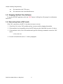
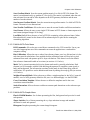
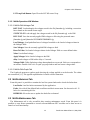
Figure 2.4: WFS Display. Each box represents the calculation
grid for each sub-aperture.
Show Vectors. Draw small vectors representing the average slope value for each sub-aperture
Show ID. Draw the ID number for each sub-aperture
Show Boxes. Draw the calculation grid for each sub-aperture defining the WFS geometry as
defined in the positions.ini file (see section 4.1.4).
Show Pupil. Draw a circle representing the pupil size and position as defined in the rtsoft.cfg
file.
Contrast. Use the slider to adjust the display contrast.
Brightness. Use the slider to adjust the display brightness.
Reset. Reset the contrast and brightness to default values.
Zoom. Use the zoom buttons to zoom in and out.
2.1.4 MAIN>Operation>TTLoop Window
2.1.4.1 MAIN>TTLoop>File Menu
Save Loop Data Sequence. Save real-time sequences of tip tilt errors and M3 commands to
disk.
2.1.4.2 MAIN>TTLoop>Tools Menu
TT Loop Performance. Window presenting the user with loop performance graphs. The
window is intended to be used as a diagnostic tool to study the tip-tilt compensation.
Mount Corrections. Charts presenting the corrections sent to the mount servo.
11
Rtsoft User Manual Rev 1.9, May 2011
Chapter 2:GUI Reference
LLT Corrections. Charts presenting the corrections sent to the LLT servo.
2.1.4.3 MAIN>TTLoop>Graphs Menu
Centroid Charts. Charts presenting real-time sequences of tip tilt errors plus statistics.
APD Flux Charts. Two charts presenting sequences of average flux values for each APD
module/channel.
Bias Calibration Button. Use the calibration button to calibrate the bias level for each
APD channel. Is up to the user to make sure that the APD signal is adequate for such
calibration.
2.1.4.4 MAIN>TTLoop>Loop Control Tab
M3 Loop Square LED. Indicator showing the current state of the M3 control loop.
LLT Loop Square LED. Indicator showing the current state of the LLT control loop.
Mount Loop Square LED. Indicator showing the current state of the Mount control loop.
APDs Bias Square LED. Indicator showing the current state of the bias subtraction to the APD
signal.
Operation Mode String Indicator. Current operation mode: TSNGS, NGS, TSLGS or LGS.
Error Source String Indicator. Current tilt error signal source: WFS or Probes.
Loop Time Numeric Indicator. Average tilt probes sampling period in [ms].
Rotation Numeric Indicator. Current rotator mechanical angle in degrees.
M3 Elevation Numeric Indicator. Current SOAR M3 elevation in units of [ADU]
M3 Azimuth Numeric Indicator. Current SOAR M3 azimuth in units of [ADU]
KC1 Numeric Control. Set the SOAR M3 controller gain.
M3 Loop Push Button. Open/Close the SOAR M3 control loop.
Time base x 10ms Numeric Control. The value entered multiplies the 5ms time base of the
tip-tilt real-time task to change the photon count period.
Lock GP1|GP2 Push Button. Activate the use of the selected probe to close the SOAR M3
loop on its signal.
KC2 Numeric Control. Set the SOAR mount controller gain.
Mount Loop. Open/Close the SOAR mount control loop.
KC3 Numeric Control. Set the LLT M3 controller gain.
Rtsoft User Manual Rev 1.9, May 2011
12
Chapter 2:GUI Reference
LLT Loop Push Button. Open/Close the LLT M3 control loop.
2.1.5 MAIN>Operation>DM Window
2.1.5.1 MAIN>DM>Voltages Tab
ROT FLAT. Load and apply the voltages stored in the file flattendm.cfg including a correction
factor based on the current rotator angle.
STATIC FLAT. Load and apply the voltages stored in the file flattendm.cfg to the DM.
REC FLAT. Save the currently applied DM voltages to disk using the protected name
flattendm.cfg and flattendm-YYYYMMDDTHHMMSS.cfg.
Load Voltages. Load predefined sets of voltages from disk to the Loaded voltages column in
the Voltages Table.
Save Voltages. Save the currently applied DM voltages to disk.
Reset To Value. Set Loaded voltages column in the Voltages Table to a user defined value.
Value. User defined voltage.
Apply Voltages. Write Loaded voltages to the DM.
delay. Send voltages to DM with a delay of 1 second.
Voltages Table. Table displaying voltage data updated once a second. Each row corresponds to
an actuator. Double click a row to open a pop-up window and load a new voltage value.
2.1.5.2 MAIN>DM>Graph Tab
The Graphs tab presents a typebar graph showing the voltage applied to each electrode. The values
are normalized [1,1]. This typebar representation is useful to detect saturation.
2.2 MAIN>Historical Tab
From this pane it is possible to examine the last five system faults and to check the faults chart.
Last Faults. Last five faults encountered by the application.
Faults. List with all the defined fault conditions and their current state. See the section 4.1.12
below for customizing this list.
REFRESH. Allows the user to update the faults list on demand.
2.3 MAIN>Maintenance Tab
The Maintenance tab is only accessible after entering maintenance mode. From this pane it is
possible to route direct commands to several software/hardware RTC modules and to have access to
some low level functionality.
13
Rtsoft User Manual Rev 1.9, May 2011
Chapter 2:GUI Reference
Command. Input box to enter string commands. For a complete list of the available string
commands read the RTSPM.
Response. Reply to the last command sent to a software/hardware module.
Send. Write the command entered in the Command input box to a software/hardware module.
Base Path. Real-Time software root directory.
Simulator Modes. Cluster indicator showing active simulator modes.
Simulator Engine. Open the rtsoft_simulator_engine.vi. This VI holds parameters to create an
artificial frame pattern, when the command line option -c has been selected. Read the RTSPM
for details on how the simulator engine works.
AO Loop Data. Open the rtsoft_task_loop_data.vi. This low level VI serves as a back door to
troubleshoot the software. More details in the RTSPM.
TT Loop Data. Open the rtsoft_task_tt_loop_data.vi. This low level VI serves as a back door to
troubleshoot the software. More details in the RTSPM.
Frame Data. Open the rtsoft_task_frame_data.vi. This low level VI serves as a back door to
troubleshoot the software. More details in the RTSPM.
DONE. Exits the maintenance mode. The Maintenance, Comm-Server and Comm-Client panes
will be closed as well.
2.4 MAIN>Comm-Server Tab
The Comm-Server tab is only accessible after entering maintenance mode (MAINTENANCE
button) . From this pane it is possible to monitor the single connection provided by the RTSOFT.
RTC Server Name. Key identifying the peer to peer connection in the configuration file
soar_comms.ini.
RTC Server Address. IP address where the RTC computer listens for incoming connections. It
must match the real-time computer IP address. The address is defined in the configuration file
soar_comms.ini.
RTC Local Port. Port at which the RTC computer listens for incoming connections. Defined in
the configuration file soar_comms.ini.
Incoming Commands. Queries and replies are showed here.
CLEAR. Clear the Incoming Commands list.
2.5 MAIN>Comm-Client Tab
The Comm-Client tab is only accessible after entering maintenance mode (MAINTENANCE
button) . From this pane it is possible to monitor the two client connections provided by the RTSOFT:
TCS and LM.
TCS Manager. Open the TCS manager task window. The window presents the messages going
back and forth between the TCS and the RTSOFT.
Rtsoft User Manual Rev 1.9, May 2011
14
Chapter 2:GUI Reference
LM Manager. Open the LM manager task window. The window presents the messages going
back and forth between the Lase Module and the RTSOFT.
15
Rtsoft User Manual Rev 1.9, May 2011
Chapter 3:Common Operations
Chapter 3:
Common Operations
Most of the time the real-time software will be ready to use on startup because the loaded
configuration files will set all typical operation parameters, (e.g. reference spot positions, reconstructor
matrix, etc.). This section outlines some common procedures involved in changing or redefining those
parameters when needed.
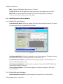
3.1 Calibrating the Wavefront Sensor
Calibrating the WFS involves three major steps: setting the exposure time, taking a bias reference
and setting the reference spot positions.
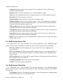
Figure 3.1: Bias Calibration Tool
To set the exposure time open the WFS GUI in the Control tab and enter a exposure time value.
Normally this value will be set to 0 [ms]. Then take a bias reference frame using the Bias Calibration
tool (Main>WFS>Tools>Bias Calibration, Figure 3.1). Finally set the reference spot positions. Select
the Modal Estimation tab in the WFS GUI (Main>WFS) and press the Set All References button. Check
the new references by looking at the Zernike Coefficients table; all coefficients should be close to 0.
The OPD representation should look flat.
IMPORTANT: The reference spot positions should be measured at the same exposure time that
will be used under closed loop operation. Otherwise spot position offset effect can distort the
slopes measurement.
3.2 Obtaining the Reconstructor Matrix H*
The process of obtaining the reconstructor matrix H* starts by measuring the interaction matrix H.
To measure H, open the Loop GUI in the Interaction Matrix tab. Then select Get Interaction Matrix to
17
Rtsoft User Manual Rev 1.9, May 2011
Chapter 3:Common Operations
open the measurement window. Enter the test voltage (typical value is 5 volts) and press start. Wait
while the program poke each DM electrode and average the slope measurements on each sub-aperture.
This might take a bit more than a minute. When the process ends the new H Matrix will be loaded into
memory. Save it for later use.
The next step depends on what type of reconstructor is to be used: Modal or SVD. Normally, the
modal reconstructor will be used. Select the Modal Reconstructor tab and press Get Modal
Reconstructor to obtain the H* matrix. If happy with the result apply it by selecting Apply
reconstructor Matrix.
3.3 Saving AO Loop Data Sequences
An important feature of the real-time software is the tool for saving loop data sequences to disk. To
save loop data sequences open the Loop GUI and select Save Loop Data Sequence from the File menu
(Main>Loop>File>Save Loop Data Sequence). The Loop Data Recorder window pops up. Enter a file
name and press REC to start recording data. The Time Recording indicator shows the elapsed time and
the File Size indicator shows how many Kbytes have been recorded so far. Press Stop to quit recording
data.
3.4 Examining the AO Loop Performance
The Loop Performance window is available to examine in detail the AO loop performance. Open the
Loop GUI and select the Loop Performance tool from the Tools menu (Main>Loop>Tools>Loop
Performance).
The software task behind the scenes continuously collects loop data (slopes and voltages) to
estimate atmospheric parameters and loop performance. When sufficient samples have been collected,
the several estimates are calculated and the collecting cycle starts over again. A progress bar indicator
to the right gives feedback to the user on the state of the samples collection cycle. The duration of each
cycle will depend on the loop frequency but in general it should take a few seconds to finish.
The Power Spectrum pane presents the user with a graph of the averaged power spectrum for both
the compensated and uncompensated signal for the currently selected mode. A control to the top allows
to select the displayed mode.
The ACF pane presents the autocorrelation function corresponding to the averaged power-spectrum
for both the compensated and uncompensated signal, for the currently selected mode. The displayed
mode is again selected with the selector control to the top of the window.
The crosses on top of the solid line representing the ACF for the uncompensated signal (e.g.
atmospheric disturbance) represent the extrapolation of the ACF to zero to estimate the WFS noise
contribution. Right now the parameters for this extrapolation (starting point and polynomial fit order)
are hard coded but suitable controls have been provided to allow for testing.
The graph in the Residual pane presents the estimates for the atmospheric variance, the residual
variance of the corrected modes and the WFS noise variance, versus mode number.
The graph in r0 and V pane presents the ratio between atmospheric variance and Noll variance for
each mode. The average of this values is used to obtain the seeing estimate r0.
Rtsoft User Manual Rev 1.9, May 2011
18
Chapter 3:Common Operations
3.5 Poking the DM Electrodes
The DM GUI is accessible from the Main GUI. When opened it presents the user with a table
containing the current voltages applied to the DM. To poke an electrode double click in the table line
corresponding to the electrode voltage you want to modify (first column lists the electrode number). A
small window will pop-up to enter the new voltage. Enter the new electrode voltage and press OK.
Now the voltage is listed in the Loaded column. Press the Apply button to actually write the voltage to
the DM.
19
Rtsoft User Manual Rev 1.9, May 2011
Chapter 4:Configuration Files and Macros
Chapter 4:
Configuration Files and Macros
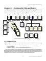
Configuration files provide a mean to set multiple system parameters to some predefined value.
Some of the parameters can be changed by the user during run-time (exposure time, reference spot
positions, etc), others will remain fixed and can only be changed by editing the files and restarting the
real-time software application (WFS pupil size, number of DM actuators, etc.). A detailed description
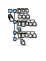
of the configuration files, macros, and their parameters follows.
rtsoft.cfg
zlabel.ini
zstatic.ini
camera.cfg
flatten
dm.cfg
initrtc.mc
faults.ini
status.ini
Xgrid.fits
Ygrid.fits
Weight.fits
positions.ini
imat.fits
initeev39.mc
rmat.fits
positions
bgnd.ini
mask.fits
apdmap.ini
bias.fits
bim.fits
eltrdmap.ini
cmat.fits
viserver.ini
dynamic
vis.ini
soar
comms.ini
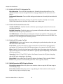
Figure 4.1: Configuration files and macros dependencies
4.1 Configuration Files
Most configuration files follow a common format. Files are divided in multiple sections, each one
beginning with a keyword enclosed in square brackets. Each section lists a parameter name followed by
an equal sign and its value. A semicolon marks the beginning of a short parameter description.
[Section Keyword]
Parameter = Value ; this is the parameter description
Other files are ordinary text files containing a list of space separated fields. The name and path of
these files is fixed and can not be modified since they are hard coded in the real-time software. Some of
these files have keywords to point to other configuration files which can have user defined names. All
configuration files are expected to live in the directory /home/ao/RTsoft/ConfigFiles.
21
Rtsoft User Manual Rev 1.9, May 2011
Chapter 4:Configuration Files and Macros
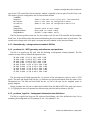
4.1.1 rtsoft.cfg – real-time software parameters
This file is currently composed of three self-explanatory sections: General, RTCORE and Simulator.
The user can hand-edit this file to modify parameter values and the name of some definition files
(interaction matrix, reconstructor matrix, bias, frame mask, reference spot positions, electrodes map,
influence functions). The following is a typical example of how this file looks like.
[General]
TELESCOPED_M=4.1
LAMMDA=0.5E-6
MODES=56
PUPILX=40
PUPILY=40
PUPILD=80
LENSLETD=8
LENSLETDM=200E-6
LENSLETFM=5E-3
PIXELM=24E-6
SD_AVERAGE=20
TOLERANCE=0.05
GAIN=1.17
PROBESCALE=1.0
M3ELSCALE=
M3AZSCALE=
;Telescope diameter in [m]
;Wavelength in [m] for calculations
;Modal estimator max Zernike mode (Mz + 1)
;Pupil center on CCD in x [pixels]
;Pupil center on CCD in y [pixels]
;Pupil diameter on CCD [pixels]
;Lenslet diameter on CCD [pixels]
;Lenslet diameter [m]
;Lenslet focal distance [m]
;Pixel size [m]
;Values to average for H matrix measurement
;Default tolerance for inverting H (SVD)
;Gain in electrons per ADU
;Translate probe centroid to arc-seconds
;M3 elevation scale in [asec/ADU]
;M3 azimuth scale in [asec/ADU]
[RTCore]
MODE=TSNGS
FRAMESIDE=80
FRAMESIZE=6400
SUBX=8
SUBY=8
MIRROR=CILAS
AV=60
MINV=-10.0
MIDV=0.0
MAXV=10.0
AOFIFOSIZE=
TTFIFOSIZE=
;Operation mode: TSNGS, NGS, TSLGS, LGS.
;Frame side in pixels
;Frame size in pixels
;Sub-aperture side in X [pixels]
;Sub-aperture side in Y [pixels]
;Mirror type [CILAS|OKOTECH]
;Number of actuators. Max is 60.
;Min low voltage in DM DAC
;Mid low voltage in DM DAC
;Max low voltage in DM DAC
;Size of the AO data FIFO buffer
;Size of the TT data FIFO buffer
[Simulator]
GRIDSIZE=80
SPUPILX=40
SPUPILY=40
SPUPILD=80
NXSUB=10
INFXFILE=
;Size of the sim-engine arrays [samples]
;Number of sub-apertures per side
;Influence functions
For example, when doing tests with DM37 the parameter AV, number of DM actuators, was set to
37; for DM60 AV is now set to 60.
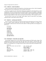
4.1.2 camera.cfg – WFS CCD controller parameters
The RTSOFT partially recycles software modules written for other SOAR applications. That is the
Rtsoft User Manual Rev 1.9, May 2011
22
Chapter 4:Configuration Files and Macros
case for the CCD controller Labview interface module, originally written as part of the ArcView code.
The camera.cfg is the configuration file for that software module.
[CAMERA]
asmpath=
macropath=
initmacro=
;Path to the boot files (files with .lod extension)
;Path to the start up configuration macro
;Name of the start up configuration macro file
[IMAGE]
ImagePath=
ImageRootName=
ImageNumber=
;Default path to save frames
;Root name for saved frames
;Default frame number suffix
The first section specifies where the low level binary code for the CCD controller and its interface
board lives. It also defines where the camera initialization macro lives and the name of such macro. The
second section keeps track of the path, root-name and suffix number of the last saved frame.
4.1.3 flattendm.cfg – voltage values to make de DM flat
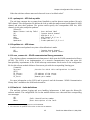
4.1.4 positions.ini – WFS geometry and reference spot positions
This file is a regular text file with each line defining a sub-aperture related parameter. The file
contains as many lines as defined sub-apertures exist.
28.000 4.000 -0.213 0.500 1.900 1.900
36.000 4.000 -0.100 0.452 1.900 1.900
44.000 4.000 -0.200 0.432 1.900 1.900
52.000 4.000 -0.235 0.345 1.900 1.900
20.000 12.000 -0.075 0.574 1.900 1.900
28.000 12.000 -0.254 0.522 1.900 1.900
36.000 12.000 -0.113 0.471 1.900 1.900
44.000 12.000 -0.324 0.478 1.900 1.900
52.000 12.000 -0.230 0.469 1.900 1.900
.......
The first and second fields represent the x-y position of the sub-aperture center in units of CCD
pixels. The third and fourth fields are the x-y reference spot position measured from the center of the
sub-aperture box. The fifth and sixth fields are the x-y size of the spot for the weighted center of
gravity template.
During run-time this file can be edited and reloaded from the Main>WFS>File menu (see section
2.1.2). Typically the user will measure the reference spot positions and save them to this file.
4.1.5 positions_bgnd.ini – background subtraction box definitions
This file is a regular four lines text file with each line defining a box. Box definition in line 0 is for
estimating the background in CCD quadrant 0, line 1 for quadrant 1, etc.
23
Rtsoft User Manual Rev 1.9, May 2011
Chapter 4:Configuration Files and Macros
4.1.6 zstatic.ini – static aberrations
If the user has selected to apply static aberrations to the reference spot positions, then the magnitude
of the aberrations for each Zernike mode will be extracted from this file.
The file is a regular text file with each line indicating the magnitude of the aberration for a given
Zernike mode. The line contains as many lines as defined Zernikes exist, but the number of them to be
considered by the software is defined by the maximum number of modes as defined by the MODES
keyword in the rtsoft.cfg file (read section 4.1.1 above). If the number of Zernikes defined is smaller
than the maximum number of modes, then the missing Zernike aberrations will be assumed to be zero.
The first field in each line is the Zernike mode number, and the second field is the standard
coefficient value for the Zernike in units of microns.
4.1.7 zlabel.ini – zernike mode label file
This is an ordinary text file listing a text label associated with each Zernike mode. Several GUIs use
this list to present Zernike related data, like the modal estimation coefficients for example. It is
recommended to match the size of this list with the number of modes specified in the rtsoft.cfg file in
section 4.1.1
TiltY(a2)
TiltX(a3)
Defocus(a4)
Astig45(a5)
Astig0(a6)
Comma(a7)
Comma(a8)
Trefoil(a9)
Trefoil(a10)
Spherical(a11)
Astigm.5th(a12)
Astrigm.5th(a13)
....
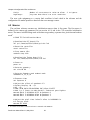
4.1.8 eltrdmap.ini – electrodes look up table
The real-time computer has two DAC boards installed to generate the DM electrode voltages. This
configuration file defines the look-up table that maps DAC board channel to DM electrode. Each
section in the file has a label with the electrode number. The section entries specify the correspondent
board (0 or 1) and channel (0 to 31), upper and lower limit for that electrode and its initialization value.
[General]
Name="Electrodes Look-Up Table"
[0]
Board=0
Channel=0
UpperLimit=10
LowerLimit=-10
Value=0
Rtsoft User Manual Rev 1.9, May 2011
;
;
;
;
;
;
;
24
User defined label
Electrode Number
Board number
Channel Number
Channel upper limit [V]
Channel lower limit [V]
Default value [V]
Chapter 4:Configuration Files and Macros
When the real-time software starts each electrode is set to its default value4.
4.1.9 apdmap.ini – APD look up table
The real-time computer has a counter board installed to read the photon counts produced by each
APD channel. This configuration file defines the look up table that maps counter board channel to APD
channel and micro-lens quadrant. The section entries specify the correspondent APD box, APD
channel, tip-tilt probe, and probe quadrant5.
[General]
Name="Counter Look-Up Table" ; User defined label
[0]
; Counter board channel
Box=
; APD Box 0 or 1
APD=
; APD Channel 0,1,2 or 3
Probe=
; Probe 1 or 2
Quadrant=
; Probe quadrant 1,2,3 or 4
4.1.10 apdbias.ini – APD biases
Loaded on boot and updated every time a bias calibration is made.
[0]
Bias=
; Counter board channel
; APD Bias in photon counts
4.1.11 soar_comms.ini – SOAR communicaton library parameters
The real-time software communication infrastructure is built upon the SOAR communication library
(SCLN). The SCLN is an implementation of a network communication layer that suites the
interoperability requirements of the SOAR telescope environment. Each section in the configuration
file for this software module defines a client-server pair with the corresponding listening port.
[CommLib]
Version=
[RTC]
IP_Server=
IP_Client=
IP_Port=
;Version for which this configuration is usable
;IP address of the server
;IP address of the client
;Remote port number
For more information on the SCLN and its protocol read the document “SOAR Communication
Library New” available at the SAM web site archive.
4.1.12 faults.ini - faults definitions
The real-time software logging and error handling infrastructure is built upon the HistoryLib
software module. The configuration file for that module defines error codes and their corresponding
error messages.
[0]
ID=
What=
;Fault identification number
;Short description of the fault
4 For information on voltage generation read the RTSPM.
5 The convention for quadrants follows that one described in SDN2306.
25
Rtsoft User Manual Rev 1.9, May 2011
Chapter 4:Configuration Files and Macros
Limit=
LogAlways=
;Number of occurrences to raise an alarm. -1 to ignore.
;Log even when there's no error condition.
The error code assignment to a certain fault condition is hard coded in the software and the
configuration file makes possible to hand edit the error message content.
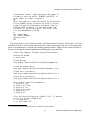
4.2 Macros
The real-time software executes two initialization macros when it first starts. The first macro is
defined in the camera.cfg parameter file (see section 4.1.2) and is the CCD controller initialization
macro. The macro initialize things such as the detector geometry, exposure time, pixel time and readout
mode6.
# SOAR TTG Initialization Macro
# Download the PCI board file
ldf pci /home/ao/RTsoft/Boot/pci+int.lod
# Reset the controller
reset controller
# Stop camera idle
readout stop-idle
# Download the Timing board file
ldf tim /home/ao/RTsoft/Boot/tim.lod
# Power on
power on
# Detector geometry
set size 80 80
# Detector Geometry and readout mode
readmode 11_12_21_22
# Exposure time
set exposure 0
# Adjust the offset of quadrant 0-3
# Guider Display: Q0 - Q1
# Q3 - Q2
# SBN Card# DAC# VID=0x564944 DAC_Value 0-0xFFF
# Add 1 or 2 Counts to make Darker / Substract goes Lighter
mancmd SBN 0 2 0x564944 0x7f2 # Quadrant 0
mancmd SBN 1 2 0x564944 0x7ea # Quadrant 2
mancmd SBN 1 3 0x564944 0x7d1 # Quadrant 3
# Adjust the pixel time. Default value is 0x180000 for
# 2.5us per pixel.
mancmd SPT 0x18
6 For details on the macro contents and macro commands read SDN8215.
Rtsoft User Manual Rev 1.9, May 2011
26
Chapter 4:Configuration Files and Macros
# Continuous readout. 2048 represents the number of
# frames in the ring buffer. 8388607 (0x7FFFFF) is
# the number of frames to capture.
##
NOTE: the number of frames multiplied by the detector
# size (80x80) and by the bytes per pixel (2 bytes)
# CAN'T exceed the high memory allocated. Look for
# BUFFER_SIZE in Memory.c in the astropciAPI_LIB
# library for the current value. Last time I look
# it was 4000x4000x2 = 30.5Mb
#
set frames 2048
set readout 8388607
exposure start
EOF
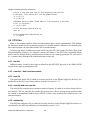
The second macro is the real-time software initialization macro initrtc.mc. This macro is the last
initialization done by the real-time software before it enters operational mode. So it is the appropriate
place to set parameters or override some default parameter values7. Right now the initrtc.mc macro is
the place for setting the centroid algorithm and defining the loop control law.
# Real-Time Computer Software Initialization Macro
# Reset the RTCORE
rt aofg reset
# Load APD map
load apdmap /home/ao/RTsoft/ConfigFiles/apdmap.ini
# Load the weight matrix
load wmat /home/ao/RTsoft/ConfigFiles/Weights.fits 1
# Load the x grid matrix
load xgrid /home/ao/RTsoft/ConfigFiles/XGrid.fits 1
# Load the y grid matrix
load ygrid /home/ao/RTsoft/ConfigFiles/YGrid.fits 1
# Set digital controller parameters
rt aofg di k 0.25
rt aofg di kl 0.999
rt aofg sp k 1.0
rt aofg sp kl 0.999
rt aofg sp ks 0.7
rt aofg sp on
# Set the centroid algorithm (1=WCoG, 5=CC). CC pattern
# size is 2.0 pixel (sigma 0.85)
rt cc algorithm 5
rt cc ref8 1000 0.85
7 For details on the macro contents and macro commands read the RTSPM
27
Rtsoft User Manual Rev 1.9, May 2011
Chapter 4:Configuration Files and Macros
# Size of the spot and size of the weighting function for
# the WCoG. This values will set the gamma factor.
rt cc NT 1.1
rt cc Nw 2.0
# Readout Noise in ADU (1.696 ADU for 1.06 us/pixel; 5.011 ADU
# for 2.5 us/pixel)
rt cc Nr 5.011
# Turn the bias substraction on
bias on
# Turn background subtraction on
rt cc bgnd 1
4.3 FITS files
Many of the program variables of the real-time software have a matrix representation. This includes
the interaction matrix H, the reconstructor matrix H*, the DM influence functions, the centroid grids,
the centroid weights, the bias frame and the Noll covariance matrix.
All these type matrix variables are stored in disk using the FITS file format. The data is kept in the
RTsoft/ConfigFiles directory. For historical reasons the names of the FITS files containing default
matrix data are defined both by suitable keyword values in the rtsoft.cfg parameter file (see section
4.1.1), and by direct loading in the initialization macro initrtc.mc.
4.3.1 bim.fits
Influence matrix. Loaded at boot time as defined by the INFXFILE keyword in the SIMULATOR
section of the rtsfot.cfg configuration file.
4.3.2 cmat.fits – Noll covariance matrix
4.3.3 imat.fits
The interaction matrix file is loaded at boot time and lives in the RTsoft/ConfigFiles directory. It is
produced from the AO Loop Control window described in section 2.1.1.1
4.3.4 rmat.fits and nas_rmat.fits
The rmat.fits file contains the reconstructor matrix elements. Is loaded at boot time along with the
nas_rmat.fits. The nas_rmat.fits file contains the reconstructor with the average slopes subtracted and
its creation is automatically handled by the RTSOFT when a new reconstructor is obtained out of an
interaction matrix.
4.3.5 wfsbias.fits
The WFS bias calibration file is loaded at boot time and lives in the RTsoft/ConfigFiles directory. It
is produced by the WFS bias calibration tool described in section 2.1.2.2.
Rtsoft User Manual Rev 1.9, May 2011
28
Chapter 4:Configuration Files and Macros
4.3.6 mask.fits
This is a matrix of dimension 80x80 in which each pixel is a 16 bit integer. Bits 15 to 8 represent the
sub-aperture ID. Bits 7,6 represent the amplifier number. Bit 4 represents the type of pixel (0 regular, 1
background). Bit 0 represents the pixel status (0 bad, 1 good).
New masks can be created using the WFS>Mask Tool (see section 2.1.2.2) and files background.ini,
badpix.fits and amps.fits.
4.3.6.1 badpix.fits
This is matrix of dimension 80x80 in which good pixels are represented by a 1 and bad pixels by a
zero. The file is loaded automatically by the WFS>Mask Tool when the user creates a new bitwise
frame mask (see section 2.1.2.2)
4.3.6.2 amps.fits
This is matrix of dimension 80x80 in which each pixel has a value of 0, 1, 2 or 3 depending on the
readout amplifier they belong to. The file is loaded automatically by the WFS>Mask Tool when the
user creates a new bitwise frame mask (see section 2.1.2.2)
4.3.7 weight.fits, xgrid.fits, ygrid.fits
Weighted center of gravity definitions. All loaded at boot time by the initrtc.mc macro.
29
Rtsoft User Manual Rev 1.9, May 2011
Chapter 5:Simulator Modes
Chapter 5:
Simulator Modes
The RTSOFT has basically two layers of simulation: a user space simulation layer and a kernel
space simulation layer. Without getting into the internals of the real-time software we can say that the
user space simulation layer involves having all the simulation done by the Labview part of the real-time
software. The kernel space simulation layer involves having the simulation done by the Labview part
plus the RTCORE8.
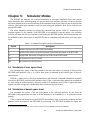
The active simulation modes are selected by command line options. Table 5.1 summarizes the
available options. So for example, if the RTCORE is not available, by giving option -r the real-time
software will start and will not complain on not finding the RTCORE present, and its functionality will
be emulated by the Labview part of the RTSOFT, that is, simulation will take place at the user space
layer.
Table 1: Command line options to the realtimesoftware.
Option
Description
-r
Emulate real-time core (RTCORE) functionality
-c
Emulate WFS camera. An artificial pattern is generated and passed to the RTCORE
-d
Emulate DM. Electrodes voltages are not written to the DAC boards.
-tcs
No connection to the TCS server.
-lm
No connection to the LM server.
5.1 Simulation at user space level
The command line option -r has been passed to the real-time software at startup. At this level the
RTCORE (and hardware if the -c or -d have been given) is emulated in the Labview part of the realtime software.
With the -r option active, the slope measurements and electrode commands calculations normally
done by the RTCORE, are done at the emulation layer. If the -c option has been passed, the calculations
are done using an artificial pattern; otherwise actual CCD frames are used. If the -d option has been
passed, electrode voltages are calculated but never written to the DAC board.
5.2 Simulation at kernel space level
The command line option -r has not been passed to the real-time software. At this level the
RTCORE is fully operational but some or all the hardware is not available (-c or -d options have been
passed).
If the -c option has been given to the RTSOFT, the emulation layer continuously produces artificial
patterns which are passed to the RTCORE for processing. The RTCORE measures the slopes and
8 For background on the internals of the real-time software read the RTSPM and document SDN8211.
31
Rtsoft User Manual Rev 1.9, May 2011
Chapter 5:Simulator Modes
voltages as under real operation. If the -d option is given, the electrode voltages are calculated but
never written to the DAC board.
5.3 Simulation Parameters
Some of the simulation engine parameters are available at the rtsoft.cfg configuration file (see
section 4.1.1 above). Other parameters can be changed by the user from the Maintenance>Simulator
Engine window under maintenance mode (see section 2.3 above).
The simulator engine includes a model of the deformable mirror (DM) based on the influence
functions defined in the FITS file given in rtsoft.cfg.
The emulated electrode voltage together with the user defined mode selected (Zernike, FITS file,
etc.) define the characteristics of the generated artificial pattern. This calculations can be intensive in
CPU resources so be aware of the lower frame rates obtained when under simulator mode.
Noise. Add white noise to the artificial pattern using the readout noise number given in the
RTSOFT configuration file.
Gain. Multiplying factor to the artificial pattern generated it can be tuned to obtained the
desired amount of flux in each subaperture.
Zernikes. Standar Zernike coefficients used to add aberration to a perfectly flat wavefront.
File. Name of a FITS containing a CCD frame.
Dark. Add the bias frame to the generate pattern to emulate the CCD bias pattern.
Mode. Read below.
5.3.1 User defined pattern
When this mode is selected the user is free to defined the values in the array representing a CCD
frame. The user can poke values and then see the results in the WFS display window. This can be very
useful when it is necessary to give a known value to a pixel.
5.3.2 5.3.2 FITS file
When this mode is selected, a user defined FITS file containing a CCD frame is loaded and used as
artificial pattern.
5.3.3 Zernike Modes
In this mode the user specifies a set of standard Zernike coefficients to add known aberrations to a
perfectly flat wavefront.
5.3.4 Kolmogorov
In this mode the spectrum of the artificial pattern follows the Kolmogorov law for atmospheric
turbulence. Correlation between successive frames is not supported though.
Rtsoft User Manual Rev 1.9, May 2011
32
Chapter 6:Log Files
Chapter 6:
Log Files
When the RTSOFT first runs, it opens a regular text file to save log messages describing runtime
events. Events can be of several types including type alarm, type command, type status, and type
simple-event. For details on the implementation of the logging mechanism read the RTSPM.
The events and the conditions in which a log message is generated is hard-coded into the RTSOFT,
but certain flexibility exists when it comes to define error messages associated to error codes. A
configuration file called faults.ini (section 4.1.12) exists that serves as a look up table between error
codes and error messages. The logging engine, when given an error code, searches the right error
message and then produces the corresponding log message.
The actual log file can be found under directory RTsoft/Logs which is typically a link to a user
defined directory (right now /home/ao/Logs). Each line in the log file starts with a timestamp that
includes date and time in YYMMDD HH:MM:SS format. Then a label describes what type of event
(alarm, status, etc.) the log message refers to. A second label states the name of the “originator”, that is,
the piece of software code that produced the event. This second label is most useful for debug
purposes. The line ends with the log message describing the event. This last message does not follow a
predefined format.
We use the system utility log rotate to manage the ICS log file. The configuration file is in
/etc/logrotate.d/icsoft.
% cat /etc/logrotate.d/icsoft
/home/ao/ICsoft/Logs/*.log {
compress
daily
rotate 7
}
The above keeps the last seven days logs in compressed format. The logrotate utility is executed as a
crontab job by the cron daemon on a daily basis (see /etc/cron.daily/ directory for logrotate). We
adjusted to run at midday
% cat /etc/crontab
# run parts
01 * * * * root run_parts /etc/cron.hourly
00 12 * * * root run_parts /etc/cron.daily
22 12 * * 0 root run_parts /etc/cron.weekly
42 12 1 * * root run_parts /etc/cron.monthly
NOTE: The whatis database update has to be removed!!
6.1 Type Alarm Events
Events of type alarm produced by the real-time software can trigger the alarm flag. Each error code
defined in the faults.ini configuration file has an associated counter that keeps track of consecutive type
alarm events. When three alarm messages in a row for a given error code are detected, the global alarm
flag is raised. The number of type alarm events in a row is actually configurable in the faults.ini
configuration file (see section 4.1.12 above).
33
Rtsoft User Manual Rev 1.9, May 2011
Chapter 7:Glossary
Chapter 7:
Glossary
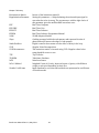
AO
Adaptive Optics.
AOSOFT
SAM Adaptive Optics Software. Supervisory control application that
handles the bussiness logic of the SAM instrument.
Deformable Mirror.
Digital Signal Processing.
Data Acquisition.
Maximum order compensation for a given reconstructor matrix.
Flexible Image Transport Format.
Full Width at Half Max.
Ground Layer Compensation
Slopes in x and y are related to aberrations by the gradient matrix G.
Inverse of the gradient matrix G.
Interaction matrix.
Reconstructor matrix.
Digital controller. Measured residuals are added to the previous signal
with some gain.
The relation between the WFS and the DM in an AO system is
characterized by the interaction matrix H.
The Kolmogorov model of the turbulence distortions prescribes the
specific form of the phase structure function for the optical wave.
Laser Guide Star
Laser Launch Telescope
Zernike mode coefficients
Error signal delivered by the WFS is converted into modal amplitudes by
matrix G*. Amplitudes are weighted and transformed to voltages by
matrix P*.
Natural Guide Star
Noise propagation is described by the covariance matrix of Zernike noise
coefficients.
Optimal modal reconstructor. Takes into account the information on the
statistics of the input disturbance contained in the Noll covariance
matrix, and correlated centroid noise.
Matrix Aberrations are related to DM voltages by the projection matrix P.
Matrix Inverse of the protection matrix P.
Modular instrumentation standard based on CompactPCI developed by
National Instruments with enhancements for instrumentation
DM
DSP
DAQ
Effective Compensation
FITS
FWHM
GLC
G Matrix
G* Matrix
H Matrix
H* Matrix
Integrator
Interaction Matrix
Kolmogorov Law
LGS
LLT
Modal Coefficients
Modal Reconstructor
NGS
Noise Propagation
Optimal G* Reconstructor
P
P*
PXI
35
Rtsoft User Manual Rev 1.9, May 2011
Chapter 7:Glossary
Reconstructor Matrix
Regularization Parameter
RTC
RTCORE
RTSOFT
RTSPM
SAM
Slope
Smith Predictor
SVD
SVD Reconstructor
TTP
TURSIM
WFS
WCoG Method
Zernike Coefficients
Inverse of the interaction matrix H.
Setting this parameter > 0 helps balancing the noise and input signal in
case when the noise is strong. The reconstructor with the right choice of
this parameter gives the smallest RMS wavefront error.
Real Time Computer
Real Time Core
Real Time Software
Real Time Software Programmer Manual
SOAR Adaptive Module
Gradient averaged within the sub-aperture and expressed in units of
phase difference between the edges of sub-aperture.
Digital controller that counter acts the effect of delay in the loop.
Singular Value Decomposition
The interaction matrix is inverted using SVD. Singular values below
some threshold are set to zero.
Tip Tilt Probe
Turbulence Simulator
Wavefront Sensor
Weighted Center of Gravity. Improved center of gravity with different
weight to each pixel depending on their flux.
Input disturbance, correction and residuals are represented as coefficients
of Zernike modes.
Rtsoft User Manual Rev 1.9, May 2011
36