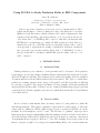
1
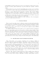
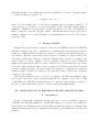
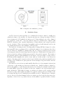
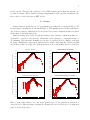
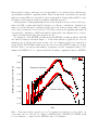
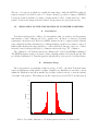
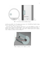
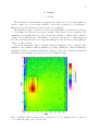
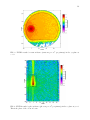
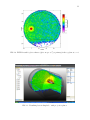
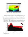
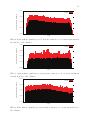
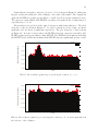
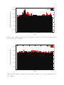
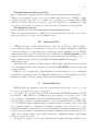
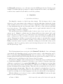
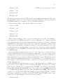
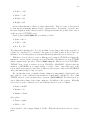
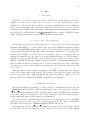
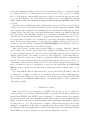
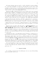
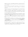
Using FLUKA to Study Radiation Fields in ERL Components
Jason E. Andrews
Department of Physics and Astronomy,
University of Washington, Seattle, WA, 98195
(Dated: August 11, 2010)
Various components of particle accelerators are sources of ionizing radiation. These
radiation fields must be considered during the design of the Energy Recovery Linac
(ERL) at Cornell University, so that the radiation can be shielded against and so that
activation in the shielding components is understood. To model the fields, the use
of the Monte Carlo code FLUKA[1] will be explored. This will be the first time that
FLUKA has been implemented to evaluate the ERL designs at Cornell. Therefore,
instructions on the use of FLUKA and its accompanying software will be created
as an appendix, to supplement the existing documentation. Radiation calculations
have previously been performed with the Monte Carlo code MCNPX[2]. Several of
these problems will be recalculated with FLUKA, and the results of the two codes
will be compared.
I.
A.
INTRODUCTION
Radiation Fields
Ionizing radiation poses a hazard to both personnel and to electronics. Beta particles,
being charged, are directly ionizing. Gamma radiation ionizes indirectly via the photoelectric
effect and Compton scattering. Free neutrons are also indirectly ionizing; there are a number
of neutron-nucleus reactions which result in radioactive nuclei. The degree to which these
particles are ionizing depends on the energy of the particle, and this dependence is different
for each type of particle. The energies and fluxes of betas, gammas, and neutrons thus well
characterize the radiation field. Various doses are obtained from flux using energy dependent
conversion tables. It is the quantity equivalent dose which characterizes the biological hazard
of a radiation field.
B.
Sources of Flux
In an accelerator environment, there are many causes for beam particles to strike the
surrounding structure. These may be unwanted causes such as beam scraping, or deliberate
causes such as collimation. When a high energy electron or positron is incident on a dense
medium, an electromagnetic cascade occurs. The incident, or “primary” lepton produces
high-energy photons via bremsstrahlung when the primary is deflected by the electric field of
an atomic nucleus. When such a high-energy photon is incident on a nucleus, conservation
of momentum allows for pair production to occur. The resulting electron and positron can
then be energetic enough to lose energy via bremsstrahlung. Hence, in a dense medium, the
2
bremsstrahlung and pair production processes feed one another in a chain reaction, producing many “secondary” particles which may escape the medium and constitute a radiation
field[3].
A neutron flux is also produced by the bremsstrahlung photons of the cascade. In addition
to pair production, a photon with energy greater than the nucleon binding energies may cause
nucleons to be ejected when the photon is incident on a nucleus. There are three primary
mechanisms by which a nucleus may be stimulated by a photon to emit a neutron—in this
context referred to as a photoneutron. These are the giant nuclear dipole resonance in the
5–15M eV photon energy range, the pseudodeuteron reaction in the 50–150M eV range, and
the intranuclear cascade at photon energies above 140M eV [4].
The relevant flux and energy calculations are thus calculations of the electromagnetic
cascade and of photoneutron production.
C.
Calculation Methods
There are special cases where it may be efficient to analyze the radiation field analytically,
but the general case of calculating cascades in a realistic environment is prohibitively complex
for an analytical solution to be obtained[4]. Such complex systems are readily modeled by
the Monte Carlo method, and it is the use of the Monte Carlo simulation software FLUKA
which is presently explored.
A calculation using the Monte Carlo method probes a physical system by tracking the
history of a single primary particle and all generated secondaries, using probability density
functions to randomly determine the outcome of particle-matter interactions. This process is
repeated for many primaries, and from the statistics of this repeated sampling, the simulation
results converge to the average behavior of the system[5]. FLUKA and similar Monte Carlo
codes employ fundamental models and enforce conservation laws to the extent that complex
phenomena such as cascades emerge extemporaneously from the physics of the simulation[6].
II.
MONTE CARLO CALCULATIONS AND FLUKA
Using a Monte Carlo code to perform a calculation can be as simple as defining an
appropriate input and running the simulation. The quality of such a calculation, however,
is not to be taken for granted. We can think of Monte Carlo calculations as characterizing
physical systems by exploring momentum space for each given real space region and for each
particle species of interest. With this in mind, a sense of ‘completeness’ can be established for
a Monte Carlo calculation, a more complete calculation being one that thoroughly probes
the relevant regions of a generalized phase space, and thus well characterizes the system
at hand. The completeness of a calculation is the degree to which the resulting data has
converged to the average behavior of the system.
In practice, this convergence is impractically slow. There is usually a large variance in
the histories of the primary particles, requiring a large number of primaries to be tracked
before the average behavior emerges. Furthermore, tracking a single primary can take a
3
significant amount of processing time given the complexity of cascades. A useful quantity
to consider is thus the computer cost,
computer cost = σ 2 · t,
where σ 2 is the variance and t is the mean computing time per primary particle[7]. If
a problem is to be calculated in a practical amount of time, then this quantity must be
minimized. FLUKA is a general–purpose particle transport code, and consequentially it
must be tailored to suit the problem at hand. This means that it is up to the user to
minimize computer cost, because the method of its minimization is subject to the details of
a given problem.
A.
Biasing in FLUKA
Biasing is the means by which computer cost is reduced in FLUKA. An un-biased FLUKA
simulation samples from ‘true’ distributions of particle-matter interactions and particle
transport, resulting in histories which are meant to accurately represent the histories of
real particles. However, such realistic histories may be dominated by physics which leave
out regions of phase space that are of interest, relegating these regions to be sampled only
in rare events, ie., a large computer cost for a quantity of interest. A ‘biased’ simulation
samples from distributions which are biased, either in favor of aforementioned rare events,
or in some other way which aims to reduce computer cost. Every particle that is tracked
is given a statistical weight, and these weights are adjusted to compensate for whatever
biasing is applied. In this way, biasing does not alter the solution, but how the calculation
converges to the solution.
Most biasing techniques reduce one factor of computer cost while increasing the other,
and it is up to the user to apply biasing such that the net computer cost is reduced. With
both FLUKA and MCNPX, the fully un-biased, or “analogue” functionality is available to
the user, as well as the methods used to bias these analogue simulations[6][5].
III.
SIMULATION OF AN ELECTRON INDUCED CASCADE IN LEAD
A.
Introduction
A basic problem with a minimal geometry is chosen to serve as an initial comparison
of FLUKA and MCNPX simulations. The FLUKA input is a recreation of one written by
Vaclav Kostroun. Calculations are performed with and without biasing to see firsthand how
different biasing methods affect computation performance of the simulations, as well as the
statistics.
4
FIG. 1: Diagram of the simulation geometry.
B.
Simulation Setup
A 2GeV electron beam is incident on a cylindrical lead target centered coaxially in a
cylindrical volume of dry air (Fig. 1). Leptons and photons of energy less than 6.737M eV
are not transported. 105 primaries are run per cycle. Neutron fluences out of the column of
air—referred to as the “lab”—and out of the Pb target are calculated and compared with
MCNPX calculation data. Spatial distributions of neutron fluence and energy deposition
are also calculated. These are measured in multiple axial and radial intervals, and in only
one angular interval due to the symmetry of the problem.
Two methods of biasing are used. Leading particle biasing (LPB) is designed to reduce
the mean CPU time per primary (t) by reducing the number of secondaries produced in a
cascade. This is accomplished by transporting only one of the two particles produced in an
electromagnetic interaction involving leptons and photons. Which particle is transported is
chosen at random, with probabilities proportional to the particle energies. The weight of
the surviving particle is then multiplied by the inverse of its probability of being selected.
LPB thus greatly simplifies the cascade event, with an obvious sacrifice of an increase in
variance. By using particle energies as selection probabilities, the particles presumably most
relevant to the calculation are given preference in an attempt to keep the variance increase
at a minimum.
Photonuclear cross sections are much smaller than those for electromagnetic interactions
of photons, so photoneutron production is relatively rare. Lambda biasing is designed to
increase the number of photonuclear interactions by reducing the inelastic nuclear mean
free path (MFP) of photons, and thereby reduce the computer cost for photoneutron spectrum calculations. With lambda biasing, secondaries are always created at photonuclear
interaction points, with weights determined by both the actual creation probability of the
secondaries and the factor by which the photon MFP is reduced. This increases t, but there
is not a direct feedback mechanism between secondaries produced and the photons producing them, so there is not a geometric increase in the number of particles tracked, as there
5
is in a cascade. Therefore the reduction of t by LPB is much greater than the increase of t
by lambda biasing. Where lambda biasing is implemented in the present calculations, the
factor used to reduce the photon MFP is 0.02.
C.
Results
Neutron fluences (particles per cm2 per primary) as a function of energy (GeV) for different biasing combinations are shown in Figure 2. The quantity plotted is the total fluence
out of the lead target. Statistical errors are plotted in red and computation times are listed
in the titles of the individual plots.
Lambda biasing alone gives exceptional neutron data, but the computation time is—
as should be expected—the greatest. Individual cycles averaged a computation time of
47.8 minutes, but some random number seeds gave cycles that did not complete even after
14 hours. Furthermore, the target dimensions are small considering the radiation length
and Molière radius of lead[8]. In calculations where a more substantial fraction of the priNo biasing, 155 minutes
Neutrons per square cm per primary
0.01
Lambda biasing, 239 minutes
0.01
0.001
0.001
0.0001
0.0001
1e-05
1e-05
1e-06
1e-06
1e-07
1e-07
1e-08
1e-08
1e-09
1e-09
1e-10
1e-07
1e-06
1e-05
0.0001
0.001
0.01
0.1
1
Leading particle biasing, 6.69 minutes
0.01
1e-06
1e-05
0.0001
0.001
0.01
0.1
1
LPB and lambda biasing, 7.25 minutes
0.001
0.0001
0.0001
1e-05
1e-05
1e-06
1e-06
1e-07
1e-07
1e-08
1e-08
1e-09
1e-09
1e-10
1e-07
0.01
0.001
Neutrons per square cm per primary
1e-10
1e-07
1e-06
1e-05
0.0001
GeV
0.001
0.01
0.1
1
1e-10
1e-07
1e-06
1e-05
0.0001
0.001
0.01
0.1
1
GeV
FIG. 2: Total neutron fluence out of the target (particles per cm2 per primary) as a function of
energy (GeV) for different biasing combinations. Statistical errors are plotted in red. Computation
times are listed in the titles.
6
mary particle’s energy contributes cascades, the number of secondaries tracked will increase
exponentially, as will the computation time. This is an important consideration for any simulation not using LPB, but especially for those using lambda biasing without LPB because
the number photoneutrons tracked are further artificially increased.
Leading particle biasing significantly increases the statistical errors for most of the spectrum, but LPB together with lambda biasing is an effective combination. Statistics are
improved over the un-biased calculation for the upper end of the spectrum, while becoming
worse only for neutrons below about 5keV . The large reduction in computing time makes it
clear that the combination of LPB and lambda biasing will be the efficient choice for more
complex calculations involving photoneutron spectra.
A comparison of the MCNPX calculation and the FLUKA calculation using both LPB
and lambda biasing is shown in Figure 3. Total neutron fluences (particles per cm2 per
primary) out of both the lead target and the “lab” air column are plotted as a function of
energy (GeV). The FLUKA results are plotted in red and the MCNPX results are plotted
in black. Both codes ran the same number of primaries, and the computation time of 7.25
minutes for FLUKA is to be compared with the 27 minute computation time for MCNPX.
0.01
FLUKA
MCNPX
Neutrons per square cm per primary
0.001
Fluences out of target
0.0001
1e-05
1e-06
1e-07
Fluences out of lab
1e-08
1e-09
1e-10
1e-08
1e-07
1e-06
1e-05
0.0001
GeV
0.001
0.01
0.1
1
10
FIG. 3: Total neutron fluence (particles per cm2 per primary) as a function of energy (GeV) out
of the target and out of the lab, as computed by FLUKA and by MCNPX. The FLUKA result
took 7.25 minutes to compute and the MCNPX result took 27 minutes.
7
The two codes give plots which are roughly the same shape, while the MCNPX results for
neutron energies below 10keV tend to be cleaner. It may be possible to improve FLUKA’s
low-energy neutron statistics by using a biasing method called “weight windows,” where
particle creation and transport in user defined energy ranges are given preference[6].
IV.
SIMULATION OF THE COLLIMATION OF TOUSCHEK PARTICLES
A.
Introduction
Touschek scattering is the collision of beam particles with one another, and the momentum transfer of such collisions can lead to particle loss. In linear accelerators, Touschek
scattering is often ignored[9]. However, in ERL designs, the more compact particle bunches
cause a higher Touschek scattering rate, so this mechanism of particle loss cannot be ignored.
Rather than allowing the stray particles to collide with the beam pipe, they are occluded
from the beam by strategically placed collimators such as the type “M” collimator.
The collimation of Touschek particles in collimator M7 of the Cornell ERL is simulated.
The FLUKA input is again a recreation of that originally written by Vaclav Kostroun. The
probability distribution of Touschek particles (shown in Fig. 4) is provided by Chris Mayes.
B.
Simulation Setup
The beam particles are initialized with an energy of 5GeV , and their Touschek distribution is implemented with particle weights. Primaries are initialized at random locations
within the distribution and the normalized probability of that location becomes the statistical weight of the particle. The transport cutoff for leptons is set at 4.67M eV and the photon
0.14
0.12
Probability
0.1
0.08
0.06
0.04
0.02
0
-1.25
-1
-0.75
-0.5
-0.25
0
0.25
0.5
0.75
1
1.25
x (cm)
FIG. 4: Probability distribution of Touschek particles incident on collimator M7.
8
FIG. 5: Geometry used in the simulation input.
cutoff is set at 1M eV . 2.5 · 106 primaries are run per cycle. Both LPB and lambda biasing
are used, with the lambda factor set at 0.01.
The 3D modeling software SimpleGeo[10] is used to create the simulation geometry. A
diagram of the geometry is shown in Figure 5. The beam particles travel in the positive z
direction. The collimator is centered at the origin of the coordinate system, and a cutaway
of the collimator geometry is shown in Figure 6.
FIG. 6: Cutaway of the collimator geometry.
9
C.
Results
1.
FLUKA
The calculation took 118 minutes to complete and consisted of 7 cycles. Neutron fluences
in the xz plane at y = 0 are shown in Figure 7, and in the xy plane at z = 0 in Figure 8.
Fluences are reported in units of neutrons per cm2 per primary.
Photon fluences in the xz plane at y = 0 are shown in Figure 9, and in the xy plane at
z = 0 in Figure 10. Fluences are reported in units of photons per cm2 per primary. The
simulation was originally run for 5 cycles, but the photon fluences outside of the collimator
volume were excessively noisy. The number of cycles was increased to 7, which improved
the data somewhat. However, as is apparent in Figures 9 and 10, there is still significant
variance in these regions.
It is worth noting that data of spatially distributed quantities can be imported into
SimpleGeo and visualized with the simulation geometry. Examples of this are illustrated
in Figures 11 and 12. Planar and linear projections of data can be extracted during the
visualization, and multiple data sets can be loaded simultaneously.
FIG. 7: FLUKA result for neutron fluence (neutrons per cm2 per primary) in the xz plane at
y = 0. This is the plane of the electron beam.
10
FIG. 8: FLUKA result for neutron fluence (neutrons per cm2 per primary) in the xy plane at
z = 0.
FIG. 9: FLUKA result for photon fluence (photons per cm2 per primary) in the xz plane at y = 0.
This is the plane of the electron beam.
11
FIG. 10: FLUKA result for photon fluence (photons per cm2 per primary) in the xy plane at z = 0.
FIG. 11: Visualizing data in SimpleGeo with projection planes.
12
FIG. 12: Using a surface extrusion to visualize neutron fluence.
2.
Comparison with MCNPX data
The MCNPX calculation took 590 minutes to complete. The FLUKA and MCNPX data
for neutron fluence along the x-axis at y = z = 0 are shown in Figure 13, along with the
statistical errors. The FLUKA results are plotted in red and the MCNPX in black. The
units are in neutrons per cm2 per primary. The two codes give curves of roughly the same
shape, but FLUKA reports a significantly greater fluence. The statistical errors reported by
FLUKA are also greater than those of MCNPX.
Neutron fluence along the x-axis at y = 0 is shown at z = −1.9m in Figure 14 and at
z = 1.9m in Figure 15. These coordinates give plots at one meter upstream from the back
collimator face and at one meter downstream from the front collimator face, respectively.
0.001
Neutrons per square cm per primary
FLUKA
MCNPX
0.0001
1e-005
1e-006
1e-007
1e-008
-100
0
100
200
300
400
x (cm)
FIG. 13: Neutron fluence (particles per cm2 ) along the x-axis at y = z = 0. FLUKA is plotted in
red and MCNPX in black.
13
0.0001
Neutrons per square cm per primary
FLUKA
MCNPX
1e-005
1e-006
1e-007
1e-008
-100
0
100
200
300
400
x (cm)
FIG. 14: Neutron fluence (particles per cm2 ) along the x-axis at y = 0, one meter upstream from
the back face of the collimator.
0.0001
Neutrons per square cm per primary
FLUKA
MCNPX
1e-005
1e-006
1e-007
1e-008
-100
0
100
200
300
400
x (cm)
FIG. 15: Neutron fluence (particles per cm2 ) along the x-axis at y = 0, one meter downstream
from the front face of the collimator.
0.0001
Neutrons per square cm per primary
FLUKA
MCNPX
1e-005
1e-006
1e-007
1e-008
-300
-200
-100
0
100
200
300
z (cm)
FIG. 16: Neutron fluence (particles per cm2 ) along the z-axis at y = 0, one meter from the side of
the collimator.
14
Neutron fluence along the z axis at y = 0 and x = 1.5m is shown in Figure 16, which puts
the plot one meter from the side of the collimator—the center of the tunnel. The comparisons
again show FLUKA reporting greater fluence overall, as well as greater statistical errors.
The curves are again similar, with FLUKA reporting a few spikes in the downstream plot,
especially near x = 1.2m.
Photon fluences are plotted at the same locations as with neutron fluences. The plots
along the x-axis are shown in Figures 17, 18, and 19, which are at the origin, one meter
upstream, and one meter downstream respectively. The plot along the z axis is shown
in Figure 20. In some locations where the FLUKA data has converged reasonably well,
FLUKA again reports greater fluence than MCNPX. The FLUKA data is much noisier than
the MCNPX data, and the uncertainties in the FLUKA data are significantly greater overall.
1
Photons per square cm per primary
FLUKA
MCNPX
0.01
0.0001
1e-006
1e-008
1e-010
1e-012
-100
0
100
200
300
400
x (cm)
FIG. 17: Photon fluence (particles per cm2 ) along the x-axis at y = z = 0.
FLUKA
MCNPX
Photons per square cm per primary
0.0001
1e-006
1e-008
1e-010
1e-012
1e-014
-100
0
100
200
300
400
x (cm)
FIG. 18: Photon fluence (particles per cm2 ) along the x-axis at y = 0, one meter upstream from
the back face of the collimator.
15
FLUKA
MCNPX
Photons per square cm per primary
0.0001
1e-006
1e-008
1e-010
1e-012
1e-014
-100
0
100
200
300
400
x (cm)
FIG. 19: Photon fluence (particles per cm2 ) along the x-axis at y = 0, one meter downstream from
the front face of the collimator.
FLUKA
MCNPX
Photons per square cm per primary
0.0001
1e-006
1e-008
1e-010
1e-012
1e-014
-300
-200
-100
0
100
200
300
z (cm)
FIG. 20: Photon fluence (particles per cm2 ) along the z-axis at y = 0, one meter from the side of
the collimator.
16
V.
CONCLUSIONS
The neutron fluences reported by the two codes agree in Figure 3, but this is calculated
from a very basic geometry. The calculations with the more complex geometry of the M7
collimator show FLUKA reporting fluences substantially greater than MCNPX, but the
curves are nearly identical. The codes agree qualitatively, but there is further investigation
to do to determine the nature of the difference in neutron fluences. There are several models
in use for neutron transport at energies above 100M eV , so investigating how each code
transports neutrons above this energy would be a good place to start.
Making calculations with FLUKA requires a substantial familiarity with how the code
performs simulations. The relevant physics and all biasing is fully user-specified, so an effective FLUKA calculation depends on an effective input. The degree of control available to the
user means there is a significant learning curve for new FLUKA users, but the experienced
user may come to view this control as an asset. Flair, the FLUKA GUI[11], does a great
deal to organize input creation, running the code, and the analysis of data, and to some
extent it automates these processes. SimpleGeo greatly facilitates the creation of complex
geometries for use with FLUKA inputs. Its data visualization capabilities are also useful.
FLUKA’s method of calculating statistical errors involves running multiple cycles of the
same calculation. Every cycle saves a random number seed to be used to initialize the
next cycle, if one is run. This means that additional cycles can be appended to a data
set without recomputing the entire calculation. This was taken advantage of for the M7
collimator calculation, and saved about 84 minutes of computing time.
The target application of FLUKA as a multi-purpose particle transport code means that
some specialized options are not accounted for by the FLUKA developers, so such options
must be implemented by the user through custom routines. However, Fortran templates
are provided for most of the common routines a user might need. For instance, the source
particle probability distribution of the M7 collimation simulation was implemented with
modifications to the “source.f” template included with the FLUKA distribution. Flair automates the integration of such routines into the FLUKA code.
VI.
ACKNOWLEDGMENTS
I would like to thank Vaclav Kostroun of Cornell University for guiding me through the
research, teaching me a great deal about nuclear physics, providing me with MCNPX input
and data, and for letting me take my final exams in his office when I first arrived here at
Cornell. I’d also like to thank Georg Hoffstaetter, Ivan Bazarov, Lora Hine, Monica Wesley,
and everyone else at Cornell involved in this year’s CLASSE REU program for making this
REU possible, and for making it a very great summer. Special thanks to Georg, Chris
Mayes, and Don Hartill for the multiple times we went sailing on the lake. This research
was supported by the National Science Foundation (NSF) REU grant PHY–0849885 and by
17
the NSF ERL grant DMR–0937466.
[1] G. Battistoni, S. Muraro, P.R. Sala, F. Cerutti, A. Ferrari, S. Roesler, A. Fassò, and J. Ranft.
“The FLUKA code: Description and benchmarking”, Proceedings of the Hadronic Shower
Simulation Workshop 2006, Fermilab 6–8 September 2006, M. Albrow, R. Raja eds., AIP
Conference Proceeding 896, 31-49, (2007)
[2] Denise B. Pelowitz, ed. “MCNPX User’s Manual, Version 2.6.0” LA–CP–07–1473, April 2008
[3] B. Rossi. Cosmic Rays, 1964
[4] H. DeStaebler, T. M. Jenkins, and W. R. Nelson. Shielding and Radiation, chapter 26 in The
Stanford Two-Mile Accelerator, p.1030, p.1038 Benjamin, 1968
[5] J. F. Briesmeister. MCNP-A General Monte Carlo N-Particle Transport Code, Version 4C,
LA–13709–M, 2000
[6] A. Fassò, A. Ferrari, J. Ranft, and P.R. Sala. “FLUKA: a multi-particle transport code”,
CERN–2005–10 (2005), INFN/TC 05/11, SLAC–R–773
[7] Statistics and Sampling presentation from the 7th Official FLUKA Course, NEA/Paris 2008
[8] H. Bichsel, D. E. Groom, and S. R. Klein. Passage of Particles Through Matter, chapter 26
in Review of Particle Physics, Particle Data Group, (2002)
[9] A. Xiao and M. Borland. Phys. Rev. Special Topics–Accelerators and Beams. 13, 074201
(2010)
[10] C. Theis and K. H. Buchegger. SimpleGeo version 4.2.0.3
[11] V. Vlachoudis et al. Flair version 0.8.2[R1.100]
Appendix: FLUKA-By-Example and Notes
or: How I Learned to Stop Worrying and Roll the Dice
I.
INTRODUCTION
This (informal) document is intended to function as an introduction-by-example to using
FLUKA and supplementary software, and to provide a medium for me to record additional
things I’ve learned from the fluka-discuss archive. The work-flow illustrated here uses Flair
and SimpleGeo. Flair is the FLUKA GUI. Several important processes such as the implementation of user routines and the merging of multiple data runs are automated by Flair. If
gnuplot is installed, Flair can also be used for plotting data, though I often find the need to
use the gnuplot command line directly. SimpleGeo is a 3D modeler and data visualization
tool. One can export geometries created in SimpleGeo for use with FLUKA, as well as
import certain data for visualization with the geometry.
Radiation about the M7 ERL collimator is the project used in the example. The following
files are meant to accompany this document:
• Monster75.01.dat
• Monster75.01.inp
• Monster75.01.flair
• M75primaries.txt
• source.mod.f
II.
GENERAL BIBLIOGRAPHY
Official FLUKA manual: FM.pdf : http://www.fluka.org/fluka.php?id=man_onl
The FLUKA manual is a valuable reference, and its complete text is integrated into Flair.
Pressing F1 within Flair opens the FLUKA manual to the entry corresponding to the
currently selected card.
Flair quick-start: Flair.pdf : http://www.fluka.org/flair/doc.html
As of this writing, Flair has advanced beyond some details in this quick-start, but Flair.pdf
remains a good introduction to the use of Flair.
Presentations from recent FLUKA courses:
http://fluka-course.web.cern.ch/FLUKA-Course/nea2008/index.php?id=c_program
and http://fluka-course.web.cern.ch/FLUKA-Course/Lectures_pdf/
These presentations tend to provide a more complete picture of using FLUKA and Flair
together. Much of the manual is simply reprinted, though sometimes in a more expository
manner. These links change over time, so I have archived the contents of the second link
above.
19
The fluka-discuss mailing list archive:
http://www.fluka.org/web_archive/earchive/new-fluka-discuss/index.html
This is a very valuable resource once one is familiar with the basics of FLUKA. Many
common problems and some not-so-common are documented here, usually with usefully
described solutions. Users are encouraged to post their input files for examination, so this
also serves as a resource for seeing how others build their (sometimes broken!) inputs.
The SimpleGeo manual:
http://theis.web.cern.ch/theis/simplegeo/manual/manual2.htm
This is the only documentation of SimpleGeo and its plugins that I am aware of, so I have
made special effort to clearly describe SimpleGeo here.
III.
INSTALLATION
FLUKA runs only on Unix while SimpleGeo runs only on Windows. Flair is built to
run on Unix and Windows, though I have only tested it on Linux. Installation of FLUKA
is fully automated by downloading and executing the current .rpm file on the FLUKA
website (www.fluka.org). For distros that are not RPM-based, Installation.pdf from the
current course materials provides the most thorough description of the install process:
http://fluka-course.web.cern.ch/FLUKA-Course/nea2008/Lectures_pdf/
Installation.pdf
An RPM is also available for Flair at http://www.fluka.org/flair/download.html,
or for a manual install, a brief description is given in the README contained in the .tar
package for Flair.
SimpleGeo is a straightforward Windows install, but the plugins need to be manually
downloaded and unzipped into the SimpleGeo install directory. Both SimpleGeo and the
plugins are available at http://theis.web.cern.ch/theis/simplegeo/
IV.
WALKTHROUGH
FLUKA, Flair, and SimpleGeo all create additional files as they run, so it’s a good idea
to create a dedicated directory for each project.
As described in sections 2.3, 2.6, and 2.7 of the manual, the FLUKA input is an ASCII
file with the “.inp” extension. Commands are given as single or double line “cards,” each
line consisting of a card name, followed by six numbered fields named “WHAT(#),” and a
text field named “SDUM.” As will be familiar to one au fait with MCNPX or a similar MC
code, the FLUKA input essentially consists of physics settings, geometry, and scoring, with
the geometry consisting of definitions of primitive geometric bodies, followed by boolean
statements defining regions with the bodies, followed finally by material assignments for the
regions. Every geometry is surrounded by a finite “blackhole” region where particles are
‘killed’ upon entering. Every point of the geometry (ie., within the blackhole ‘shell’) must
belong to exactly one region.
For simple geometries, we can open a template and complete the input in Flair as per
20
the Flair.pdf quick-start, or we could just create the ASCII input directly. For the present
example, we assume that the geometry is complex enough that we want to use SimpleGeo
so that we have visual feedback while we create the geometry.
A.
1.
SimpleGeo
Quick-Start and Settings
The SimpleGeo interface is divided into three frames. The left frame is the boolean
algebra tree, the center frame is the working area, and the right frame displays the details
of the currently selected node in the boolean tree. SimpleGeo defines regions by implying
boolean statements from the tree hierarchy, with bodies and boolean operators appearing
as nodes in the tree. The visibility of regions can be toggled with the check-box of the
corresponding node in the boolean tree.
The middle-mouse-button (MMB) toggles between ‘move-object’ mode and ‘rotatecamera’ mode. Minimal coordinate axes are always visible in ‘rotate-camera’ mode, and
I never use ‘move-object’ mode, so I often select View→Coordinate-axes to turn off the
main coordinate axes. The scroll wheel zooms the camera and holding the RMB pans the
camera. Changing the visibility of regions will cause the camera to automatically zoom and
pan when Automatic camera is turned on under View→Camera-settings (on by default).
Ctrl+a resets the camera. I prefer to darken the working area for the sake of my eyes by
navigating to the View→Settings window and selecting Background color: Black gradient
and Background type: Full.
2.
Creating Geometry
The following instructions recreate part of the Monster75.01.dat file. One could simply
open that file and skim this section to see how it was created, or the instructions can be
followed verbatim, using Monster75.01.dat only as a reference. Upon opening the file, a
message will most likely appear indicating that the auto-update has been turned off. It can
be turned back on by selecting it at the bottom of the View menu.
Select the tab “Simple1” if it’s not already selected. This is the new project that is started
by default when SimpleGeo is launched. Select the root node in the boolean tree, then create
a difference-operation node by pressing Ctrl+Shift+D, or by selecting its icon from either
the toolbar or the Objects menu. The children of a difference node define the volume that is
the first child minus all its younger siblings. This is the only case where the order of nodes of
the same generation has meaning. This order can be changed by selecting the node to move,
then right-clicking it and selecting CSG tree tools→Reorder nodes. Hierarchy changes can
be made by selecting a node, then dragging it onto the node which will become its parent.
With the difference node selected, create a cylinder (Ctrl+Shift+C) and use the right
frame to set the following properties:
• Name = blkhole
this becomes the name of the body in the input file
21
• X-Rel = −145
FLUKA uses the unit cm for distance
• Z-Rel = −320
• Radius = 260
• Height = 640
The entry in the Comment field is NOT exported as a comment in the input file. Also note
that the number of faces of bodies is only for rendering in SimpleGeo. See section 8.2.4 of
the FLUKA manual for a description of bodies and their parameters.
Create another cylinder, again with the difference node selected.
• Name = twall1
• X-Rel = −145
• Z-Rel = −300
• Radius = 245
• Height = 600
First-generation children of the root node are interpreted as regions, and SimpleGeo
incorporates the basic FLUKA materials for regions. Materials can be assigned with the
drop-down list at the bottom of the right frame when a valid node is selected. Material
BLACKHOLE is the default, thus we have now completely defined the geometry of the
blackhole region surrounding our primary geometry. For the first-generation nodes of the
root, the name listed in the right frame becomes the name of the region. Change the name
of the difference node to BLKHOLE . Note that regions cannot share the names of materials
in a FLUKA input.
Before continuing, we must address “reference” nodes. The use of a boolean tree introduces a complication that does not exist when one simply lists bodies and declares regions
by naming the bodies in boolean algebra statements. We’ve created bodies as children of a
first-generation node (a region), but we’d like to use the same bodies in other first-generation
nodes. This is accomplished with reference nodes. Any change to a node that is referenced
will propagate down to all reference nodes. A reference node cannot, itself, be referenced,
but any other node can.
Hide BLKHOLE by un-checking the box next to its name in the tree. With the root
node selected, create a difference node and name it TUNNEL. We want to use concrete
as the material, but this is not a default material of FLUKA. We will have to modify this
later in Flair. Expand the BLKHOLE node, select twall1, hold down Shift, drag twall1
to TUNNEL using the LMB, release the LMB and finally release Shift. This creates a
reference node of twall1 in TUNNEL, which might not appear until the display is refreshed
by selecting a different node and then reselecting TUNNEL. With TUNNEL selected, create
a difference node, and with this node selected, create a cylinder:
• Name = twall2
22
• X-Rel = −145
• Z-Rel = −310
• Radius = 213
• Height = 620
Observe that this inner cylinder is longer than twall1. This is because bodies used in
boolean algebra statements must not have coplanar surfaces. For instance, if twall2 were
the exact length as twall1, then it would be ambiguous whether the points at the ends of
twall1 are part of TUNNEL or not.
Create a plane (Ctrl+Shift+P) as a sibling of twall2 :
• Name = tfloor
• Y-Rel = −140
• Rot. X = 270
Try temporarily changing Rot. X to 90, and thus observe that points on the green side of
a plane are considered to be external to the plane body while points on the red side are
internal to it. Note that planes are automatically hidden when they are not selected.
With the root node selected, create a difference node, name it TNLAIR and change the
material to vacuum. Create a reference node in TNLAIR to the difference node in TUNNEL
which contains twall2 and tfloor. That is, Shift+drag the difference node in TUNNEL to
TNLAIR. Next, create a reference node in TNLAIR to BLKHOLE . Observe that the
inclusion of BLKHOLE as a younger sibling of ‘twall2 - tfloor’ cuts off the ends of the
region, which is necessary because these points were already part of the region BLKHOLE,
and points must belong to only one region.
We can skip this action of cutting off extra volumes by using infinite cylinders and ‘cutting’ planes to create cylindrical regions instead of using finite cylindrical bodies. With
TNLAIR selected, create an intersection operation (Ctrl+Shift+I). The intersection operator defines the volume of the points common to all children of the operator. With this
node selected, create a difference node and with that selected, create a cylinder;
• Name = shell01
• Radius = 50
• Infinite = Z-axis
and a plane:
• Name = pzn90
• Z-Rel = −90
Pzn90 should be the younger sibling of shell01. With the intersection selected, create a
plane:
23
• Name = pz90
• Z-Rel = 90
This coordinate-based naming convention makes it easier to locate bodies which will be
referenced often, such as cutting-planes.
The rest of the geometry is created primarily by the methods just described. It should
be noted that there are different techniques which achieve the same geometry, and that this
has only been an illustration of one possibility. Open Monster75.01.dat if it is not already
open to continue with the example. In the tree, observe the large fraction of reference nodes
used, illustrating the utility of a good naming convention for bodies.
With the auto-camera on, hiding TUNNEL and TNLAIR makes it easier to view the
collimator regions. Take note of RING06A and the body taper01 therein. One must increase
the value of View→Settings→Nr. of property digits for greater accuracy of Radius Low and
Radius High to be exported. Note that these radii cannot correspond the the radii of
the infinite cylinders they intersect because of ambiguity this would create in the boolean
statements involving taper01, the cylinders, and cutting planes. Observing the hierarchy
of RING06A/B and BEAMAIRB may be instructive as well. As another detail, examine
shell08 in RING07A. Try changing the number of faces to see the display anomalies (on the
tapering part of RING07A) that sometimes occur in SimpleGeo. As evidenced by shell08,
changing the number of faces can fix the display. However, such anomalies are certainly not
features of the geometry exported to FLUKA, so there is no harm in ignoring them.
We are ready to export the SimpleGeo .dat model as a FLUKA input. Select
File→Export→Preferences and check Export material names. This is not necessary
but it makes the input more readable. Export it using a suitable name by selecting
File→Export→Fluka, and under Save as type:, select the parentheses input option. This
creates an incomplete ASCII input for FLUKA, which we shall complete using Flair.
B.
Flair Quick-Start
The left frame of Flair is used to select what frame is displayed on the right. The root
node Fluka should already be displayed upon launching Flair, but if it is not, select it in
the left frame or press F2. We can open a template to make a new input or we can open
an existing input. Open the input just exported from SimpleGeo by clicking on the ‘open’
icon next to the Input: field. Change the Title: field to Monster75 and click yes on the
window that pops up asking to update the TITLE card. Go ahead and save the project as
Monster75.01.flair by selecting the ‘save’ icon next to the Project: field or on the toolbar.
Press F3 or select Input in the left frame. A list of all the input cards is displayed in
the right frame, and the text of the currently selected card is displayed at the bottom as
it actually appears in the input file. Selecting different fields of the card will highlight the
corresponding WHAT(#) at the bottom. The blue lines of text at the top of some cards
are the commented lines preceding the card in the input file. Pressing F1 while a card is
selected will open the FLUKA manual in Flair to the description of that card. Note that the
24
Flair manual is integrated into this FLUKA manual, and that pressing F1 when a different
frame is selected (e.g. Compile or Run) opens the Flair manual to the relevant entry. I
find Flair to be well documented in this manual, but it does assume complete knowledge of
FLUKA.
C.
Geometry Debugging
Before making any changes to the input, it’s a good idea to debug the geometry to make
sure that we have not assigned points to more than one region or to no region at all. The
debugger is explained in the Flair manual (F1) under the entry Debug Geometry, as well as
in the FLUKA manual under the GEOEND card entry. Select Debug in the left frame, then
click the “+” icon in the upper-right of the Geometry Debugger frame twice to add two test
regions. Enter;
• Name = tunnel
• Xmin = −395
• Xmax = 105
• NX = 101
• Ymin = −250
• Ymax = 250
• NY = 101
• Zmin = −305
• Zmax = 305
• NZ = 123
for one region and;
• Name = collimator
• Xmin = −55
• Xmax = 55
• NX = 111
• Ymin = −55
• Ymax = 55
• NY = 111
this is the number of mesh points in the x direction
25
• Zmin = −95
• Zmax = 95
• NZ = 191
for the other. In some geometries, the odd number of mesh points helps to keep the points
being sampled from coinciding with region boundaries.
Select the tunnel region and select the Debug button in the lower-right. After a few
seconds the debugging will stop with errors found. Double-click the .out file to open the
standard out so we can see what FLUKA has to say. Select ERROR on the left and you
can see a large number of ‘point not contained in any region’ messages together with the
coordinates of the point. One can usually gain insight into the problem by examining the
ranges of these coordinates. In this case, there is nothing wrong with the geometry, we
have simply defined our cuboid debugging region such that it contains points outside of our
BLKHOLE region. Simply increase the radius of the RCC card for the blkhole body to
R = 360 and the debugger will now run without error. Also run the collimator debugger for
a higher-resolution check of this geometry. With these verifications complete, we can expect
to be done with SimpleGeo and can proceed with editing the input in Flair.
D.
The Minimal Input
Press F3, select the GLOBAL card, and change the Input: field to Names. The mouse
behavior can sometimes be problematic, so I often Tab through the fields of cards and select
pull-down-options with the arrow keys. Notice the brighter highlighted text at the bottom
showing when changes are made. One can press Esc to stop editing the fields of a card.
Select GEOBEGIN, change the title to Monster75, and change Fmt: to COMBNAME .
Notice that when the Fmt list is selected, the right most field of the card is highlighted at the
bottom, indicating that this is the SDUM. Press F1 to find out what using COMBNAME
does, and notice that the SDUM default for GEOBEGIN is COMBINAT . WHAT(#)s and
SDUM s left blank often take on such default values.
Flair introduces explicit REGION cards which are the region declarations in the input.
It is instructive to examine the REGION cards to see how the regions made in SimpleGeo
are expressed purely as boolean statements.
ASSIGNMA cards assign materials to regions, and SimpleGeo creates an ASSIGNMA
card for each region. For several consecutive regions with the same material, one ASSIGNMA
card can be used for the whole sequence of regions to clean up the input if one wishes. Notice
that the ASSIGNMA for TUNNEL is material BLCKHOLE, which we now update. Flair
contains a database of materials, and the author of Flair emphasizes that this is only a
reference database and that the material properties should be verified.
Select Material in the left frame to display the database. Enter concrete in the Search:
field and select Concrete portland. Either hold the RMB and release it over Insert to Input
or double-click on Concrete portland, causing a pop-up to appear. Check MAT-PROP and
then click Selected to insert the material into the input. Press F3 to return to the input
26
and notice the COMPOUND, MAT-PROP, and portland concrete MATERIAL cards. As
stated in the manual, a MATERIAL card must be present to use any material that is not
listed in section 5.2 of the FLUKA manual. Notice that Flair automatically created the
MATERIAL card for potassium, which is used in the COMPOUND card for the portland
concrete. Finally, select the ASSIGNMAT card which has the Reg: TUNNEL entry and
select PORTLAND in the Mat: list. Note that in these pull-down lists, one can press the
first letter of the desired entry to jump to that section of the list.
We now define the beam. Select the GLOBAL card, then select Card from the menu
bar or press Insert. Select Primary→Beam and a BEAM card will be inserted after the
GLOBAL card. When a *.flair is opened, Flair will move stray cards like BEAM out of
the sequence of geometry cards, but I am in the habit of putting beam-related cards at the
top of the input. Set:
• Beam = Energy
• E = 5.0
FLUKA uses the unit GeV for energy
• Part = ELECTRON
The default values are suitable for the remaining WHAT(#)s. The default beam starts at
the origin and points in the +z direction, and we override these defaults with the BEAMPOS
card. Press Insert, select Primary→Beampos and set z = −70.1. The manual indicates
that a beam should not start on the boundary between regions, hence the extra millimeter.
Next, select the last ASSIGNMA card, press Insert, and select General→Randomize.
Press Insert again, and select Primary→Start. Enter 2.5e5 in the field No.:, this is the
number of primaries used in the calculation.
In terms of required cards, we now have a complete FLUKA input, even though it’s not
very useful since we haven’t requested any scoring. The point, however, is that the example
so far has followed a completely general procedure for creating a FLUKA input that starts
with SimpleGeo. I have simply assumed a particular geometry to illustrate this procedure
with.
E.
Completing the Input
We now continue by adding the more specialized elements of the input. What remains is
to specify scoring, activate physics relevant to that scoring, optimize the running time and
statistics with biasing, and to specify a custom beam profile.
1.
Scoring
The repository of FLUKA lectures (http://fluka-course.web.cern.ch/
FLUKA-Course/Lectures_pdf/) has a good intro to FLUKA’s scoring, (c08 Scoring.pdf )
and the description of FLUKA input sections in the manual are also valuable. Many
27
questions and answers are in the mailing list archive, so it’s a good idea to search the name
of a card there to learn more about it. This example uses USRBIN and the supplementary
AUXSCORE card.
USRBIN is the FLUKA equivalent of MCNP(X)’s mesh tally. It is a grid of bins, independent of the geometry, and it can be used to score energy deposition or fluence. The
AUXSCORE card can accompany a USRBIN and convert fluence to dose during the run,
though it can be used to modify scoring other than just USRBIN.
Score cards output either binary or ASCII files. FLUKA comes with many useful routines
for processing the binaries, and Flair automates this process. Flair can also automate
the merging of multiple cycles of the same run for the purpose of calculating statistical
errors. Thus we usually ask FLUKA to output binaries and generate ASCII files afterwords.
Multiple instances of the same type of score card can output to the same file, but I find it
convenient to output to separate files when there will not be very many scoring cards.
Select Scoring under Input in the left frame. Press Insert, select Usrbin, and enter the
following values:
• Unit = 50 BIN
BIN indicates ‘binary’
• Name = nFluence
• Type = X-Y-Z
• Xmin = −395
• Xmax = 105
• NX = 100
• Part = NEUTRON
• Ymin = −250
• Ymax = 250
• NY = 100
• Zmin = −310
• Zmax = 310
• NZ = 124
Press Esc to finish editing the card, press Ctrl+c and then Ctrl+v to create a duplicate
of the card. Make the following changes:
• Unit = 51 BIN
• Name = phFluence
• Part = PHOTON
28
Notice that when the name is changed, Flair asks if we want to update anything in the
input that has referenced this name. This is useful in some cases, but nothing references the
‘detector’ we’ve just created. Finish editing the card, paste the first USRBIN again, and
make the following changes:
• Unit = 52 BIN
• Name = nDose
• Part = DOSE-EQ
Copy this third USRBIN and paste a fourth, making the following changes:
• Unit = 53 BIN
• Name = phDose
These last two USRBIN s currently score equivalent dose for all particles, so we supplement
them with AUXSCORE cards to filter just neutrons and photons. Press Insert, select
Auxscore, and enter the following values:
• Type = USRBIN
• Part = NEUTRON
• Set = AMB74
• Det = nDose
The default values of the last two options are fine, so leave them blank. Set: is this card’s
SDUM. Press F1 to see the available sets of conversion coefficients. Create a new AUXSCORE or copy and paste this one, using PHOTON as the particle and phDose as the
detector.
2.
Physics
Many physics options are set in FLUKA by using the DEFAULTS card. When the
DEFAULTS card is not present, as in the current input, the setting NEW-DEFA is assumed.
NEW-DEFA is suitable for many cases, but we must turn on photonuclear interactions
manually by creating a PHOTONUC card. Otherwise our neutron detectors won’t register
anything. Press F3, press Insert, select Physics→Photonuc, and set the following values:
• Delta resonance: on
• Quasi D: on
• Giant Dipole: on
• Mat = BLCKHOLE
29
• to Mat = @LASTMAT
We could simply set All E: = on, but for a 5GeV electron beam, this slows the calculation
with no significant effect on statistics. The @LASTMAT specifies the last material in the
list of materials used, effectively selecting the entire list.
3.
Biasing
There are several ways to implement biasing in FLUKA, and much time can be spent
tailoring the biasing techniques to a given input. Ideally, one would strike a balance between
time spent tweaking the biasing and computing time saved. There are a couple of biasing
cards that have a significant impact on performance which we shall use in the present
example, but there are also several others described in the manual as well as in the course
materials on-line.
In the Input frame, press Insert and select Biasing→Lam-Bias, then enter the following
settings:
• Part: = PHOTON
• % λ inelastic = 0.01
With these settings, LAM-BIAS reduces the mean free path for inelastic nuclear interactions
of photons, which effectively gives the simulation many more opportunities to probe the
photonuclear characteristics of the problem. Such interactions are much less probable than
photon interactions with atoms and electrons, so running a simulation using 2.5·105 primaries
and no biasing would provide very ‘rough’ and ‘sketchy’ USRBIN data for the neutron
fluences, with many bins going completely untested. LAM-BIAS certainly increases the
computing time of the simulation, but increasing the number of primaries to achieve the
same degree of convergence to the solution would correspond to a much more dramatic
increase in computing time.
Another form of biasing we will implement is called leading particle biasing (LPB), which
is designed to reduce the number of particles tracked in an EM cascade. Its use increases
the variance in some regions of phase space, which I have seen in neutron fluences below
0.1M eV . However, it drastically reduces the computing time for each primary particle.
Indeed, in this example, a cycle of 2.5 · 105 primary particles would take 66 times longer
without it. LPB is more thoroughly explained in Note 9 of section 7.2 EMF-BIAS in the
FLUKA manual.
LPB is implemented with either the EMFCUT card or the EMF-BIAS card. EMFCUT
allows us to turn on LPB as well as to set energy cutoffs for particle creation and transport.
EMF-BIAS allows us to turn on LPB with more specifications about when and where it
is applied, but presently we simply want it across the board, so we will just use EMFCUT
since we would have created that card for the cutoffs regardless.
With the Input frame selected, press Insert and select Transport→Emfcut, then enter
the following settings:
30
• e-e+ = 0.00467
• γ = 0.001
• Bremsstrahlung = On
• Pair Prod = On
• e+ ann @rest = On
• Compton = On
• Bhabha&Moller = On
• Photo-electric = On
• e+ ann @flight = On
• Reg = BLKHOLE
• to Reg = @LASTREG
The field Type: is this card’s SDUM, and should be left blank for the card to invoke LPB.
4.
A User Routine for the Beam
We want to simulate a beam with an x-distribution given by the discrete locations
and corresponding probabilities listed in M75primaries.txt. This is accomplished with
the user routine source.mod.f. A number of user routine templates are included in
$FLUPRO/usrmvax, and it is instructive to compare source.mod.f to the file source.f
found there. Source.mod.f will be called every time a primary particle is initialized in the
simulation. It will choose a line number from M75primaries.txt at random, initialize the
primary at the location in the line number, and apply a weight to the particle using the
probability of that line number.
The source routine is called by adding the SOURCE card into our input. Insert this card
at the top of the input (it’s located in Primary→Source) and leave all the options blank.
Note that BEAM is still a required card. In general, the source routine simply overrides the
specifications of the BEAM card.
As explained in section 13.1 of the FLUKA manual, we must compile the source.mod.f
file and link the resulting source.mod.o to the FLUKA routines by producing a new
FLUKA executable. These processes are automated by Flair. With source.mod.f in the
working directory of the project, press F5 or select Compile under Process in the left frame.
Click the “+” button in the upper-right and select source.mod.f and then click Open in
the pop-up. Click the Exe: field and another pop-up will appear. Enter M75fluka as the
file name and click Save. Select source.mod.f under the File list and then click the Build
button. Flair will both compile the source routine and produce the new FLUKA executable
using the name entered in the Exe: field.
31
5.
Final Details
Flair likes to interject the unnecessary STOP card at the end of an input when a project
is saved. This can effectively break an input if one saves an incomplete project and then
later inserts some cards at the end of the input. FLUKA will ignore cards that appear after
STOP, and indeed, it is this functionality that makes STOP a useful card for debugging
since one can effectively comment off the ‘bottom’ of an input. But we don’t presently need
the STOP card, so either delete it or move it to the very end of the input. When STOP
is present, the last three cards in the input should be RANDOMIZ, START and STOP, in
that order. Once this is verified, the input is complete.
Finally, place a copy of M75primaries.txt in the directory of the project, and we will
be ready to run FLUKA.
F.
Running FLUKA
Press F6 to display the Run screen. Here we can set the number of cycles in a run,
monitor its progress, and cancel a run if needed. Notice M75fluka is listed as the FLUKA
executable. When FLUKA is executed, a directory named fluka #### is created where
temporary files are stored. “####” is just the number of the process, and this directory
will be deleted upon completion of the run. Flair displays the progress of the run and of
the cycle, and it displays the cycle progress by reading the *00#.out file every 15 seconds,
where “*” is the title of the input and “#” is the number of the cycle. The time Flair waits
to check this file can be changed in the Tools→Preferences window under Project. Also
notice the Attach timeout listed there. Flair will stop checking for updates and list Timed
out as the status after this time has passed with no change to the output file. Once FLUKA
has made some progress, we can ask Flair to resume checking on the status by clicking the
Attach button.
If a run needs to be aborted for any reason—perhaps a biasing tweak has caused it to
become unreasonably languid—then one can select Stop Run. This creates a rfluka.stop file
in the fluka #### temporary directory. The file is empty, and FLUKA will check for the
existence of it every 50 primary particles or so. This means it might take FLUKA a while
to finish with the current set of primaries and stop, but it has always (eventually) stopped
for me. The temporary directory will remain when FLUKA is stopped in this manner, so it
must be removed manually if its contents are of no use.
When running an input for the first time, I usually run only one cycle and ignore uncertainties in the data so that I can just get a feel for how biasing is affecting the running
time and the ‘completeness’ of the simulation. Here we assume that our input is suitable,
so go ahead and set No. Cycles to 7 and click Run. It will take FLUKA a few moments
to initialize, and then the Primaries progress bar should begin to update. On the machine
I used, this run of 7 cycles with 2.5 · 105 particles each took about 110 minutes. For the
sake of continuing with the example, the number of primaries could be reduced to 2.5 · 103
and the run should finish in about a minute. Either way, the run should complete without
timing out and the status message Finished OK should appear.
32
G.
1.
Data
Output Files
Press F7 to view the Output Files screen. The Fortran output units as well as the
.out files for each cycle are listed, and one can view one of the output files by doubleclinking on it. One should always examine one of the output files when a new simulation
has been run for the first time, because the input is echoed there and one can see how it
is interpreted by FLUKA. The output files contain much useful information in addition to
this, and they are well explained by c09 Output.pdf in the repository of FLUKA lectures
(http://fluka-course.web.cern.ch/FLUKA-Course/Lectures_pdf/.
2.
Data Post-Processing and Merging
The binaries created by the scoring cards need to be processed by the various programs
that ship with FLUKA, or by user routines. The appropriate FLUKA programs are usually
described in the FLUKA manual entry for the score card in question, and these programs
are found in $FLUPRO/flutil. It’s important to understand what those do to the data. For
instance, the USRBDX card can be used to score fluence, and one can request only one
angular bin. In such a case, the data scored is still differential in angle, so each bin must be
multiplied by 2π to get the integrated data. However, the program usxsuw —used to merge
multiple USRBDX binaries and compute standard deviations—performs this multiplication,
thus one must not include an extra factor of 2π when plotting the data. The point is that
one must keep post-processing in mind when learning about how the various scoring cards
record data.
Flair automates post-processing and merging. Press F8 to display the Data Merging
screen. The scoring units are listed in the Usrxxx frame. Select all four of them, then click
Process in the lower-right. Flair will run the appropriate program(s), which is usbsuw in
this case. We can work with the USRBIN data in Flair or in SimpleGeo.
3.
USRBIN Data in SimpleGeo
Once this has finished, press F7 to go back to the list of output files and notice the four
* usrbin ## files listed there. These are still binaries, but we can convert any of them to
ASCII for viewing in SimpleGeo. We could have simply asked for ASCIIs when creating the
score cards, but then we would not be able to take advantage of the data merging program,
which significantly impacts the statistics of the simulation.
To convert a binary to ASCII in the Output Files screen, simply select it, hold the RMB
and then release it over the option To ascii that appears in the list. After a moment the
list of files will refresh and a * usrbin ##.lis ASCII file will appear.
Open SimpleGeo and load the DaVis 3D plugin by selecting Macros→Load plugins. Check
the box next to DaVis 3D, click Load selected Plug-Ins and close the window. The plugins
33
tend to hide themselves in the toolbar next to the ‘automatic update’ icon. Open the plugin
by clicking DaVis3D, or if this button is not visible on the toolbar, open it by clicking
the “Toolbar Options” button which appears as a vertical bar with two tiny arrows at the
top—very well disguised. See section 5.3 in the FAQ section of the SimpleGeo manual
(http://theis.web.cern.ch/theis/simplegeo/manual/manual2.htm#FAQ) if this is still
not clear.
Load the data by clicking the points of ellipsis button next to the File name field. Select
All Files in the Files of type pull-down menu, and then open the appropriate .lis file. Click
Load data and just use unity for the normalization factor in the window that pops up. After
clicking Ok, the data will be processed and another window will pop up asking for min and
max data values. The min value will have to be increased to something of order 10− 12,
otherwise most of the relevant data will be compressed into a narrow spectrum of red colors.
Projection planes are turned on by checking the boxes next to the names of the planes. Use
the scroll bars next to these names to ‘browse’ the data. Multiple data sets can be loaded by
creating a copy of the DaVis 3D plugin file (VDaVis3D.plx) in the SimpleGeo directory,
then loading this re-named file as an additional plugin.
Data can be viewed together with geometry simply by opening a SimpleGeo .dat file
after loading data. Several options that can be useful for visualization are X-Ray mode
for regions (displayed under Vis Attributes in the right frame when the region is selected),
clipping planes (in the View menu), as well as a very well-hidden option named Enforce
overlay. This last option can be found by opening the DaVis 3D window, right-clicking
the title bar, then selecting Settings from the list that appears. X-Ray mode can be too
obfuscating, so whenever I use it I also select View→Contouring→Render hard contours. To
save a screenshot for use in a presentation or paper, use the usual Windows Ctrl+Print
Scrn shortcut to copy the screen to the clipboard, then paste it into an image editor to crop
and save.
Note that with the Extract button near the bottom of the DaVis 3D window, data can
be extracted by a number of methods. A very useful extraction is Plane, which takes the
slice of data being displayed by any of the projection planes and produces an ASCII. The
data is extracted in a minimal column format, so it can immediately be used by gnuplot or
other such programs.
4.
USRBIN Data in Flair
Flair can be used to project any range of USRBIN data onto the xy, yz or xz planes, as
well as geometry cross sections. When using Flair for spatial plots like this, we must keep
in mind that FLUKA, like MCNPX, uses a left-handed coordinate system. In geometries
(such as the present one) where asymmetries make this relevant, we can circumvent this by
simply browsing for the data we want using Flair, then re-plotting it with gnuplot, applying
an extra factor of −1 to the appropriate coordinate. This is the ideal approach because
SimpleGeo is right-handed. If we were to manually mirror the geometry once it’s imported
into Flair (as well as any right-handed external data such as the source distribution), then
the FLUKA data would not display correctly with the SimpleGeo geometry.
34
An elegant, alternative approach would be to build a left-handed geometry in SimpleGeo, and modify any SimpleGeo screenshots by reflecting them across the vertical. Such
screenshots don’t have labels to act as fingerprints of the image mirroring operation. Note
that this would still require that we mirror any right-handed external data, which could be
easily done with a −1 factor in the source.mod.f routine.
Anyways, press F9 to display the Plot List screen. Profiles of plots can be generated
automatically by clicking the “Scan input file for possible plots” button on the right, which
has an icon that looks like a gear. Click this, and notice that plot nodes appear for geometry
and for each of the USRBIN units in the left frame. Select the node corresponding to unit
50 to display the USRBIN Plot screen. Enter −1 in the aspect: field to set the x and y axes
to the same scale. In the Projection & Limits section, set the z limits at 0 to 5. Z should
already be toggled as the axis to project. Leaving the x and y limits blank defaults them
to their min and max values. The Norm: field takes a numerical factor or expression to
multiply the data by. Notice that the Geometry: Use: pull-down is set to -Auto-, meaning
Flair will generate and overlay a geometry plot. This will be a cross section of the geometry,
occurring on the projection axis at the coordinate given in the Pos: field. When this field
is blank, the cross section occurs at the middle value of the projection limits—2.5cm in this
case.
Click Plot in the lower-right. Flair will generate a * usrbin 50 plot.dat file and a
* usrbin 50 plot geo.dat file, which are ASCIIs of the projected data and the geometry.
Flair then sends plot commands for these to gnuplot, which should pop up without error
if gnuplot is installed. Labels can be added to this plot with the Axes Labels section (CB
stands for ‘color bar’), and gnuplot commands for these labels can be added in the relevant
Opt: fields. A plot produced in this screen can be saved by clicking in the File: field at the
top of the screen.
I often find it necessary to work with gnuplot directly. For instance, as mentioned above,
Flair will naı̈vely plot the present projection as though the coordinates were right-handed.
Thus I want to apply a factor of −1 to the x coordinates, but there is no way to add this
with the Flair interface. Flair is still of use though, because in such cases, we can use it to
generate the *plot.dat and *plot geo.dat files from the binary data, then work with these
in gnuplot. Of course, we could save some time and just choose to live with left-handed plots,
but this method illustrates how we can take advantage of Flair’s methods to extract ASCII
data from the binaries without working with the large ASCIIs that we send to SimpleGeo.
To get a view from the top, toggle y to be the projection axis in the Projection & Limits
section, set the y limits at 0 to 5, and reset the z limits to blank values (or the full z domain,
of course). To plot this rotated 90◦ , check the box next to swap and set the Geometry: Axes:
pull-down to X-Z.
V.
VARIOUS NOTES
Not everything got integrated into the walk-through, so here are some additional things
that are very useful to know about.
35
◦ Multiple projects can be opened simultaneously in Flair by selecting File→New Window and opening the project there. Note that one can copy and paste cards from one
project to another.
◦ Cards can be temporarily disabled in Flair by right-clicking a card and selecting Disable
Card(s) in the pop-up menu. This is very useful for debugging or for experimenting
with biasing.
◦ Additional cycles can be run and merged with data from a run that has already
completed. We might want to do this if uncertainties are too large overall, or if the
simulation does not appear ‘complete’ enough. To do this in Flair, go to the Run
Fluka screen, set the Previous field to the number of the last completed cycle, then set
No. Cycles to the number of cycles being added. Once these cycles complete, simply
re-process the data in the Data Merging screen.
Note that if USRBIN plots have already been generated, then we will have to make
whatever change is necessary in the USRBIN Plot screen to cause Flair to re-generate
the *plot.dat and *plot geo.dat files from the new binary data. If we were to make
a plot, re-process the binaries, then make another plot without any changes, Flair
would just use the previously existing ASCII files created when the original plot was
made.
◦ USRBDX, USRTRACK, and similar scoring cards should be requested to output binaries. When Flair processes and merges the cycles, the ASCII files * usr* ## sum.lis
and * usr* ## tab.lis. are created. the ‘sum’ file contains a somewhat expository
summary of what was scored, while the ‘tab’ file is the raw data formatted for use
with software such as gnuplot.
◦ When Flair uses gnuplot, the commands issued to gnuplot appear in the Flair output terminal. This can be a valuable way to learn gnuplot commands by example,
even though Flair’s commands to gnuplot can be redundant. These output terminal
commands can also give insight into how the raw data is formatted.