Download User guide

OPA version 3.39
Andreas Streun, PSI, March 14, 2012
1
Introduction
1.1
Status
OPA is under continuous development, but some colleagues all over the world like to use it,
therefore these instructions have been written.
Incomplete features or known problems are described using italics.
1.2
General information
OPA’s main purpose is to support the development of electron (positron) storage rings. Emphasis is on visualization and interactivity. OPA is in particular useful for designing high
brightness light source lattices, but may be used for transfer lines and other types of lattices
as well. Storage ring design with OPA starts from scratch and ends at a bare (i.e. error free)
lattice with optimized 2D dynamic apertures, to be passed on to other codes like TRACY or
MAD, which use more complete models.
1.3
History and acknowledgements
OPA is based on the code OPTIK from Klaus Wille (DELTA/Dortmund), who started in the
80’s already to work on a design tool for electron rings. In 1993 he kindly passed it on to
the author, who developed it further and heavily used it for the design of the Swiss Light
Source, SLS. Algorithms for sextupole optimization and signal processing were contributed by
Johan Bengtsson (now BNL). Simon Leemann (MAX-Lab) did a lot of tests and suggested
many extensions and changes during the design of MAX-IV. Michael Borland (APS) tested the
module for non-linear optimization for consistency with the ELEGANT code and helped to
find several bugs.
1.4
Capabilities and limitations
OPA includes the following features:
• Human readable lattice input/output and robust lattice reader.
1
• Text editor and modular editor for elements and segments.
• Interactive graphical design of linear optics with many convenient functions as knobs,
zoom, matching, tune diagram etc.
• Calculation of momentum dependent lattice parameters.
• Interactive optimization of sextupole and octupole Hamiltonian in 1st and 2nd order.
• Tracking with FFT: Poincar plots, resonance guesses and amplitude dependent tunes.
• Tracking of dynamic apertures.
• Tracking of Touschek lifetime.
• Display of lattice geometry.
• Orbit distortion and correction.
• Calculation of magnet currents and export of EPICS snap files.
• Export of TRACY, MAD-X and ELEGANT lattice files.
• Several ways to export graphics: image snapshots, export as *.wmf file, export of *.gp
file for GNU-plot
• Export of data in text files.
OPA has the following limitations:
• Only correct for rings with large circumference and high energy:
− High relativistic approximation: γ 1
− Paraxial approximation: x = dx/ds 1
− Large curvature approximation: x ρ (bending magnet radius)
• Exactly correct only on energy (i.e. ∆p/p = 0), since it uses internally x0 instead of the
canonical coordinate px .
• No betatron coupling and no skew elements included, i.e. it allows only flat lattices.
• Nonlinear elements are treated by a 2nd order symplectic integrator only.
• Only planer insertion devices allowed. Simple model as dipole array.
• Only 4D tracking (no synchrotron oscillations).
• Approximative (not exact) calculation of path length and dipole down-feed from higher
multipoles (contribution to radiation integrals).
2
2.1
How to use
Installation and files
OPA is a Windows program, best tested for XP. There is no special installation procedure:
OPA is one single executable opa.exe and does not need additional libraries or files to run.
2
Table 1: Files read or written by OPA
file
read write
files in the OPA folder:
opa3 path.ini
•
•
remember last used files
[diagopa.txt]
•
[code development]
files in each data folder:
opa3 set.ini
•
•
user settings for this folder
(name).opa
•
•
lattice files
•
plot export as Windows metafile
(name) (plot).wmf
(name) (plot).txt
•
plot data export as text file
(name) (plot).out
•
plot data export as text file
•
GNU plot command file for plotting *.out
(name) (plot).gp
(name).lat
•
TRACY lattice file
(name).mad
•
MAD-X lattice file
for EPICS export of magnet currents (in data folder):
allocation.opa
•
power supply allocation
calibration.opa
•
magnet calibrations
(name).snap
•
EPICS snapshot file
[(name).dev]
•
[outdated]
So all to do is to create a folder for OPA and perhaps one or another for the data. Note, that
OPA needs write permission also for the folder where it is located, so it does not run from a
CD. Table 1 gives an overview of files read or written by OPA.
2.2
Start
The OPA menubar gives access to all functions. The large buttons on the GUI access only
the most used functions. If functions are not available, because a prerequisite is missing (e.g.
periodic solution for tracking) the buttons are disabled and shown in gray.
”Active file” shows the selected lattice file (*.opa). A lattice file contains a list of elements
(magnets) and a list of segments. A segment is a series of elements and segments (see section 3
for definition of elements and segments).
The ”active segment” is selected from the segment list on the GUI. From this segment, the
lattice is built by recursive expansion of the segments to get the elements line-up, which is
shown in the message window when pressing ”show lattice”.
Upon start only the ”File” and ”Edit” options in the menu bar and the corresponding buttons
are enabled. One may either read a *.opa file or create a new one by using one of the two
editors.
3
2.3
Editor
There is the OPA editor and the text editor. New users may prefer the OPA editor, advanced
users the text editor.
The OPA Editor shows a list of elements and of segments, and further has input fields for beam
energy, element apertures and for a comment text. The functionality is quite obvious and does
not need much explanation:
The element editor allows to define the type of element and to set its parameters (see sec.3.3
for element properties).
The segment editor allows to type in the line-up of elements. Insert and Delete keys may be
used. Undefined elements are shown in red, before saving the segment they need either to be
deleted or to be defined using the element editor. The periodicity field stores a number of
repetitions of the segment, for example used to calculate tunes etc.
”Invert dipole polarities” inverts the polarity of all dipoles and combined function magnets in
the lattice.
”Set all element apertures” overwrites all element apertures with the values given in the input
fields. Warning: all individual aperture settings, if any, will be lost!
The text editor shows the file exactly as it will be saved to disk, see sec.3.1 for explanation.
The ”test” button performs a syntax check.
2.4
Design: optics
The lattice structure appears on the optics panel, and a menu to select constraints pops up:
• ”periodic” will try to find a solution with same parameters at both ends
• ”symmetric” will try to find solution with αx = αy = η 0 = 0 at both ends, so appending
the mirror image makes it periodic.
• the ”single pass” options calculate the optics starting at its left or right end or from one
of the ”optics markers” if any.
If periodic or symmetric fails, the single pass solution from initial (left) values is calculated.
If the periodic solution was found, the tune diagram pops up (see below).
Beta functions and dispersion will be shown (βx in blue, βy in red, η in green). The table at
right gives in its upper part total values of the lattice (some of them only valid, of course, if
the lattice would be repeated periodically). In the lower part, local optics values are displayed.
The location can be selected by right-clicking on the plot.
4
Moving the mouse over one of the elements displayed at the bottom of the figure shows its
name. Left-click on an element and releasing the mouse button after moving to one of the
”knob” fields, connects the most important parameter of this element to the knob. Variation
by moving the slider or entering numbers changes the optics. The range of variation is given
by the fields at the bottom of the knob, which are adjusted automatically, but can be changed
using the ”<>” and ”><” buttons.
Left double-click on an element opens the panel from the element editor which allows to change
all parameters.
Buttons at the top of the plot allow to zoom in: calculation through elements proceeds in slices
of length corresponding to 1 pixel on screen.
The button field at lower left:
”Start” again selects the constraints.
”Envelopes” is for showing the beam size: if the equilibrium values of the lattice are used, an
emittance coupling factor has to be given, since there is virtually no vertical emittance in an
ideal flat lattice. The envelope plot will show the 1-sigma beam size and the element apertures.
Dispersion is included in the horizontal beam size, its contribution shown as a dashed line.
”Momentum” displays the optics for ±∆p/p and on-momentum. One may select to include
sextupoles or not. Click Momentum again to switch off this mode. Note, that a sextupole
connected to one of the knobs of course can only affect the off-momentum curves.
”Tune Matrix” gathers quadrupoles in two groups depending on the sign of the k-value and
establishes a sensitivity matrix for a relative change of strength. This allows relatively smooth
tuning of the lattice within a small range.
”Matching” opens the panel for iteratively adjusting beam parameters. Matching can be done
from any location to another in the lattice, i.e. begin, end or optics markers. Constraints at
an intermediate marker may be added.
On the left panel, select parameters to adjust and enter target values. On the right panel,
select elements to be used for matching. If the number of elements is equal or larger than the
number of constraints, the ”go” button is enabled and matching may start.
The algorithm is a Newton search using the inverse square sensitivity matrix of the most effective
knobs as tangent for extrapolation (see K.Wille’s book). This method converges quadratically
but is rather fragile. Reducing the ”fraction” of iteration to be applied stabilizes. Other parameters are number of iterations and required precision for termination.
If the iteration was successful, one may watch the solution (”show”), ”accept” or ”reset” it to
the initial. ”retry” returns to the first screen to change the settings and try again.
Known bugs: Symmetric or periodic option does not yet work well. Previously selected intermediate constraints are not reset on restart.
”write OMK” writes the current optics into the optics markers elements, which can be selected
on a panel that will pop up.
5
”Print” prints the plot stretching it to the available area and refining it to the available resolution of the selected printer.
”→Plot” writes a graphics file (nam) beta.wmf with betafunctions, resp. (name) envel.wmf
if envelope mode was selected.
”→txt” writes a text file (nam) beta.txt of plotted data (for postprocessing using other tools).
”→GP” writes text files (nam) beta.out with the beta functions and (nam) mcod.out with
element data to be read by a GNU-plot command file (nam) beta.gp, which is also created.
Running GNU-plot on this file (outside OPA) then will create an EPS file (nam) beta.eps.
”Exit” terminates the optics design. Note that the question to save the data refers only to an
internal save to further proceed inside OPA, but does not save the data to the file!
If optics design ends with a periodic solution, the options ”sextupoles” and ”tracking” become
enabled.
There is an embarrassing bug that could not yet be fixed: if the optics plot window is covered
up many times by other panels, Windows runs out of memory probably due to some OPA-bug
in repainting the plot window, and every user action will repeat this error. In the worst case,
OPA has to be killed using the Windows tasks manager.
2.5
Tune diagram
The tune diagram pops up when a periodic solution is found, it shows the working point at the
centre and the resonance lines in the neighbourhood.
The lines aQx + bQy = c to be shown are selected by the order buttons and the checkboxes:
• Order buttons select |a| + |b| ≤ order.
• ”nsys” not checked selects only systematic lines, where c mod P = 0, with P the periodicity of the lattice.
• ”skew” not checked selects only regular lines, where b mod 2 = 0.
Buttons at bottom modify the plot range.
”Export” writes a graphics file (nam) tuneplot.wmf.
Double-clicking the image saves the bitmap to the clipboard (this works for all plots in OPA
except the ”Optics Design” plot).
2.6
Design: sextupoles
Sextupoles, octupoles and decapoles may be used to optimize the dynamic aperture after chromaticity correction.
6
The modes of the sextupole Hamiltonian are calculated in first and second order, (see section 4.1): there are 10 terms in first order (2 linear chromaticities and 8 resonances) and 13 in
second (2 quadratic chromaticities, 3 amplitude dependant tune shifts (ADTS) and 8 octupolar
resonances). The first order modes of the octupole Hamiltonian are calculated and added to
the 13 second order sextupole modes. Also cubic chromaticities are calculated. Chromaticity
and path length calculation is done by numeric differentiation of the dispersive orbit, whereas
all other quantities are calculate analytically.
All Hamiltonian modes are normalized to betatron amplitudes of 2J = 1 and a relative energy
deviation of ∆p/p = 1. ADTS values are displayed as ∂Q/∂(2J).
As much as possible is calculated only once at start of the sextupole module. This may cause
some delay depending on the total number of sextupole kicks in the lattice (which depends on
the number of slices per sextupole etc.). But afterwards the iterations will be fast.
A tune diagram will also pop up. In addition to the tune diagram opening with linear optics,
it shows the expected tune spread of the beam: the magenta/cyan parabola shows the tune
variation due to chromaticity and the green straight lines due to betatron amplitudes.
The sextupole panel lists at left the 25 Hamiltonian modes plus a sum of total sextupole
strength. The numbers are the absolute value of the (complex) mode and given in SI-units. To
each resonant mode exists a complex conjugate, which is not shown.
The ”periods” field will be set to the number of periods of the lattice, but may be changed to
study how the resonant terms vary due to interference. For the non-resonant terms, the period
number is just a scalar multiplication factor. A value of 0 means ∞ and is applied only to the
resonant terms, of course.
The bars are for comparison and visualize the contribution to the minimizer’s penalty function,
they are products of the modes’ absolute values hjklmp with relevant amplitudes (2Jx ), (2Jy )
and δ, and weighting factors: the relevant betatron amplitudes and momentum range are given
by the fields at bottom, practical units here are mm·mrad and %. Another (empirical) factor
applies to the resonant terms to make them comparable, otherwise they would be invisible
compared to the chromaticities. The weighting factors are given by (2w − 1) with w stepped
up/down by the ” + ” and ” − ” buttons. For non-resonant, additive terms like chromaticities
and tune shifts, a target value can be set. The check boxes in the ”inc” row include/exclude
the related quantities to the minizer.
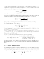
The penalty function is calculated as
X 2
(2w − 1) 10WR (2Jx )(j+k)/2 (2Jy )(l+m)/2 δ p |hjklmp − tjklmp |
jklmp
For the non-resonant mode, where =(h) = 0, a target value tjklmp can be given, which is
always zero for the resonant modes. For the resonant modes, a general weighting factor WR
is given in the fifth field at the bottom of the panel, to increase their weight, because due
to interference they are smaller numbers than the additive, non-resonant terms, but due to
resonant amplification they may be more harmful.
7
The right side of the panel shows the integrated strengthes of the related sextupole resp.
combined function magnet families. Maximum strength and step size for pressing the ” > ”
and ” < ” buttons are given below. ” >> ” and ” << ” buttons apply 20 steps. ”off” sets
to zero, ”res” restores the initial value. The ”lock” check box excludes the family from the
minimizer. Underneath are windows to set maximum strength and step size.
For automatic adjustment of linear chromaticities to the target values, two sextupole families
have to be selected by clicking the check boxes in the row labeled ”ξ”. If these sextupoles have
no dispersion, chromaticity correction will be impossible and an error message is shown. There
may be a small deviation from the target value of chromaticity. This is due to the fact, that
linear, quadratic and cubic chromaticities are obtained from numeric differentiation, whereas
the chromatic sextupole values are calculated using the simple 2 × 2 matrix containing the well
known sums over beta functions and dispersion.
The ”select” button launches a window for visualization of the first order resonances, it displays
the sextupole kick vectors in the complex plane. Pressing ”select” again toggles between the
8 resonance modes which will be highlighted at left. The sum is shown as circle. An 8th plot
shows the sum vectors of the 8 resonance modes for comparison.
If there are octupoles in the lattice, they will be shown underneath the sextupoles, and a row of
checkboxes labeled ”O” appears besides the 2nd order chromaticities and amplitude dependant
tune shifts. Checking these boxes activates a singular value decomposition (SVD) routine [7]
which is controlled by the buttons appearing underneath the octupoles: The ”Condition” and
”Nweight” labels shows the ratio of smallest non-zero to largest value of the weight vector
and the number of non-zero values. The −/+ buttons may be used to filter these values and
improve the condition. The ”SVD” button performs a calculation which can be canceled using
the ”undo” button. Checking the ”auto” box enables automatic SVD after each change of
a sextupole. SVD uses all available octupoles, but checking the ”lock” box at an octupole
excludes it.
If there are decapoles in the lattice, they will be shown underneath. They only affect the cubic
chromaticites and may be modified manually only.
A cubical fit for the momentum dependant orbit length (longitudinal chromaticity) is given
at the bottom, numbers given are the first three orders of the momentum compaction factor
multiplied by the lattice length.
”start” starts the minimizer, which uses the Powell algorithm [7]. The initial step size for
sextupole variation may be set. The minimizer will inform on its progress by listing the current
value of the penalty function (normalized to its start value) and also by writing messages to the
message window on the OPA main panel. After successful termination, the penalty function is
shown in blue, after interrupt in magenta.
The minimizer does not use the octupoles, however if the ”auto” option for SVD is activated,
the octupoles are set after each minimizer step. In the same way the chromaticity sextupoles
are set.
8
”Exit” terminates the sextupole programs and asks if the new sextupole values should be saved.
Note that the question to save the data refers only to an internal save to further proceed inside
OPA, but does not save the data to the file.
2.7
Tracking: phase space
This panel shows Poincaré plots of particle motion in horizontal and vertical phase spaces (x, x0 )
and (y, y 0 ) (it is x0 , y 0 although the axis are labeled px , py ). The circles or ellipses show the linear
acceptance given by the physical aperture. When starting a particle, the effective apertures are
also shown, which are reduced due to coupling assuming elliptical beam pipes (see sec.4.5).
By left-clicking in the diagrams or by entering numbers in the centre panel, the starting conditions are selected. A momentum deviation may be entered in the ”dp/p” field. ”run” tracks
the particle a number of turns as given in the top panel, ”more” adds more turns, ”clear” clears
the panel, ”exit” terminates the program.
A Fourier spectrum of particle motion is calculated after tracking and shown in the lower
diagrams. The algorithm used is FFT with sine window and sin x/x peak interpolation to obtain
frequency and amplitude of the peak in order to identify (guess) the underlying resonance [5].
Results are shown in the lower panel. The tune considered as the fundamental is also marked in
the tune diagram. The ”param” button opens a panel to set parameters for resonance guessing:
”fundamental tune range” sets the maximum deviation of the guessed tune from the linear tune.
”peak identification tolerance” sets a parameter p defining ∆Q = p/c as the maximum tune
deviation, with c the order of the resonance. The two filter levels are for accepting peaks and
for the range of the plot.
By default, tracking uses the apertures of the elements to test on particle loss. By unchecking
”element apertures”, the apertures in the ”Ax”, ”Ay” fields are used instead. Aperture check
assumes an elliptical beam pipe and tests for (x/ax )2 + (y/ay )2 ≤ 1. Note, that the aperture
check may underestimate losses, because internally, sequences of linear elements are concatenated into matrices at start. Aperture checks are only done at locations of nonlinear kicks and
at the track point. Therefore, particle tracking may also paint outside the linear acceptance
ellipse.
The trackpoint by default is at the begin/end of the lattice, but the field ”trackpoint” allows
to select any location. The ellipses indicating the physical acceptance will change accordingly.
The ”amplitude dependent tune shifts” panel performs three series of trackings stepping up the
initial angles x0 , y 0 in steps as given in the ”steps” field until the maximum betatron amplitudes
given by physical acceptance, are reached. The first (third) series goes in horizontal (vertical)
direction up to the maximum betatron amplitude with a tiny vertical (horizontal) amplitude in
order to excite coupling. The second series sets the initial coordinates for a constant coupling.
Coupling and maximum amplitudes are defined in sec.4.5.
The identified tunes are marked during execution in the tune diagram, and afterwards they
are plotted vs. betatron amplitude, or vs. ”ping”, i.e. the initial kick angle. The three series
9
correspond to the lines blue-X, lilac-X (both showing ∆νx vs. 2Jx ) and purple-Y (showing ∆νx
vs. 2Jy ) in the left diagram, and to the lines lilac-X (showing ∆νy vs. 2Jx ), purple-Y and red-Y
(both showing ∆νy vs. 2Jy ) in the right diagram.
Since the amplitude is derived from the height of the fundamental peak in the Fourier spectrum,
it may happen in case of very strong non-linearity, that the curve ”returns” towards the origin,
if a harmonic peak grows on expense of the fundamental peak. It may also happen, that the
tune gets stuck on a resonance (i.e. the particle is trapped in an island in phase space) and the
tune shift vs. amplitude shows a flat line.
If theoretical amplitude dependent tune shifts have been calculated previously in the sextupole
module, they are shown as dotted line for comparison.
2.8
Tracking: momentum
Actually, this module does no tracking but calculates the linear optics along the off-momentum
orbit. It works for periodic and also for single pass systems: the checkbox at top right makes
the selection and is checked at start if a periodic solution was previously calculated. The range
of momentum variation and the number of steps may be set, and if a periodic or single pass
solution is requested (the corresponding checkbox is set following previous ”Optics Design”
calculations). ”Go” starts the calculation. A tune diagram pops up in case of periodic solution.
Afterwards, several plots may be selected by the radio buttons at left. Each curve is fitted by
a polynomial, the order to be selected by the field at left, where also the coefficients will be
shown in a table. The ”Units” button switches between plot units and SI units for displaying
the coefficients.
In the tune plots (first four radio buttons), also the theoretical values (actually calculated in
the same way by numeric differentiation) are show by solid lines, if the sextupole module was
used before. The chromatic beam footprint will be shown in the tune diagram.
”→WMF”, resp. ”→TXT” writes a graphics file, resp. a text file of the data named
(name) momentum N.wmf, resp. .txt, where N is the number of the plot (radio button). Doubleclicking the image copies it to the clipboard.
Up to four parameters may be selected for automatic minimization by checking the box after
the name of the parameter. It then appears as a button label in the minimizer panel at
bottom. Clicking this button shows the parameter in the plot and allows to edit target values
as polynomial coefficients in the fit panel at right, which are shown in pink in the plot. The
minimizer is of Powell type [7] and works on the penalty function
XX
f
wf (f (δ) − fT (δ))2 ,
δ
with δ the array of momentum values covering the selected range, f the momentum dependent
parameter, fT the target for this parameter, and wf a weighting factor. The latter is entered left
of the button. Only nonlinear elements are available for minimization, the minimizer knobs are
10
the strengths normalized to the initial values. ”Optimize” starts the minimization, ”Break” interrupts it, ”Reset” restores the initial values. ”Plot absolute/relative” toggles between showing
parameter and target, or the difference between both.
Target values are saved on exit, however this has been implemented yet only for tunes and path
length up to 12th order.
2.9
Tracking: dynamic aperture
There are three modes: x vs. y, x vs. ∆p/p and y vs. ∆p/p. When selecting the first, a
∆p/p offset may be given, for the others it is a ∆p/p range. The plot will show the geometric
acceptance based on linear beam dynamics and the grid for probing stability by starting particles at these locations. Grid parameters may be stepped up and down by the ”cells” buttons.
The geometric acceptance is modified by setting the apertures as described in sec.2.7. Other
parameters are the number of turns (and the location of the trackpoint).
”Start” starts probing the grid: surviving particles are shown in green, lost ones in red. ”Export” writes graphic files (name) dynap xy/ xp/ yp.wmf. Double-clicking the image copies it
to the clipboard.
In x vs. y mode, the geometric acceptance is shown as a blue polygon. It is given by the common
area of the projections of all the elliptical apertures to the track point (see appendix 4.5).
This geometric acceptance includes non-linear and chromatic contributions to orbit and beta
functions but else assumes linear transformations. In tracking, it may happen, that particles
outside the geometric acceptance survive for two reasons: 1) aperture checks are only performed
at non-linear elements (because to speed up tracking series of linear elements are concatenated
and stored as matrices), and 2) the non-linear eigenfigure of betatron motion may be different
from an ellipse.
2.10
Tracking: Touschek lifetime
This module for Touschek lifetime calculation proceeds in two steps:
1. Work sheet to calculate lifetime related parameters in a linear model: one may enter parameters in the left panel and see the results in the right panel and in the plots. Available plots
include
• the beta functions,
• the lattice invariant H,
• the rms beam envelopes,
• the apertures,
• the bunch volume,
11
• the momentum acceptances from RF (green) and from apertures (brown),
• the ζ-parameter for the Touschek function (see section 4.2)
• the local loss rate in linear scale, and
• the local loss rate in logarithmic scale.
2. Tracking for local dynamic momentum acceptance: after pressing ”track”, the program will
step along the lattice in steps of ∆s and start particles on-axis but with momentum deviation
∆p/p to simulate Touschek scattering. A binary search on ∆p/p determines the minimum and
maximum values of ∆p/p accepted at the particular location. Only locations where H (and its
nonlinear equivalent) has changed need to be tested, therefore the loop jumps over non-dipole
elements and just copies the previous momentum acceptance data.
During execution, the plot will switch to momentum acceptance to show the progress of the
calculation. ”Break” allows to interrupt. When done, all calculations for ζ, loss rates and
lifetime like in the linear case are done and the results are added to the plots. In the ζ plot,
2 additional lines for positive (red) and negative (blue) dynamic momentum acceptance will
appear. In the loss rate plot it is only one line for the total losses (pos. and neg.).
Input parameters:
• Energy may be changed for testing, but the original value will be restored on exit.
• Coupling is the emittance ratio.
• Total beam current in the machine, and
• number of bunches give the charge per bunch.
• The cavity voltage defines bunch length and RF momentum acceptance. If it is lower
than the energy loss per turn, the bunch length is set to the ring circumference and the
momentum acceptance is zero.
• The harmonic number contains RF wavelength. The number of buckets can not be higher
than the harmonic number, this is checked.
• The longitudinal resolution defines ∆s for tracking along the lattice.
• Momentum resolution defines the precision of the binary search.
• Numbers of turns to track to decide on loss or survival.
• Residual gas is defined by atomic number, atoms per molecule and partial pressure.
The gray fields show quantities derived from the input values, which can not be modified.
”Track” starts the tracking, which is a 4-D tracking, i.e. keeping the momentum constant.
”Track sync” is an improvised 5-D tracking, varying the momentum deviation δ = ∆p/p in
turn k simply as δk = δo cos(2πνs k), with νs the synchrotron tune. The implementation is very
inefficient, and therefore this tracking is rather slow.
12
”Export plot” writes a file (name) touschek N.wmf, where N =0..8 is the number of the plot
(N=0 for beta function plot etc.).
”Export data” writes a file (name) touschek.txt with all plotted data.
”ZAPLAT” writes a file (name) zaplat.dat to be used as input file zaplat.dat by the ZAP
code [2] for calculation of intra beam scattering. Note, that aperture data as needed for
Touschek lifetime calculations by ZAP are not included.
2.11
Extra: Geometry
A plot of the lattice layout: press and hold the left mouse button to mark a rectangle to zoom
in. The curved arrow buttons on top will follow the lattice back or forth, the third button
zooms out again.
If there are marker elements named ”center” in the lattice, the plot will be centered at the
center of gravity of these markers.
Unchecking the ”fix aspect ratio” box stretches the plot horizontally and vertically to the
canvas, otherwise (default) same scales are used horizontally and vertically.
Parameters in the table control width (and length of some) elements.
”wmf” writes a file (file) geometry.wmf, ”data” writes three files, named markers.txt,
devices.txt and orbit.txt containing data of points where a new straight or curved section starts, the data of the ploygons relative to the markers and the data of the orbit. Markers
and orbit can be visualized by checking the corresponding boxes.
2.12
Extra: Orbit
If monitors, horizontal and vertical correctors have the special names MON, CH and CV, the family
is expanded in single elements names MONnnn etc., where nnn is a number. Only these elements
will be used for orbit correction. Correctors or monitors with other names remain families and
can only be used manually. Monitors and correctors will show on the Orbit panels as green,
blue and red objects. Correctors can be dragged to knobs to use them manually, a monitor can
be dragged to the BPM-field. It will show its reading there. By switching from ”actual” to
”Reference” a target value can be entered for x and y and is written to the BPM after pressing
”set”.
The ”status + statistics” panel at lower left allows to set the starting point and to include or
exclude nonlinear elements. The statistics panel shows mean, rms and max values for orbit
relative to reference (”BPM”), for absolute orbit at all elements (”all”) or for the corrector
kicks (”Corr”) – press to toggle.
The ”plot” panel at lower right allows to choose between corrector and orbit+BPM plots. If
”keep max.” is checked, no autoscaling of plot is done.
The ”misalign and correct” panel sets misalignments and performs orbit corrections: Misalign13
ments are entered in micron and will be applied to all magnets (not the correctors) as Gaussian
distributed random numbers with the given cut-off in sigma. ”seed” determines the series of
random numbers. ”Set” applies the misalignments, ”zero” sets them to zero, and ”re-set”
applies a previous setting again (to save retyping the input fields).
”Corr” calculates the response matrix, sets-up the SVD and performs orbit correction. The
results as shown below the ”Corr”-button are:
”COD”: no correction done,
”zeroed”: success: orbit agrees with reference,
”minimized”: success: orbit does not agree with reference, but does not converge any further.
This is typically the case if there are less correctors than monitors.
”no convergence”: failure: too many iterations, the orbit loop did not converge.
”failed”: complete failure, beam ran off.
The buttons ”Corr=0” and ”BPM=0” set all correctors, resp. all BPM references to zero.
The figure displays the SVD weight factors, where the excluded (zero) values are shown darker.
The small button toggles ”X” and ”Y”, and the slider allows to reduce the weighting factors.
OPA may crash and get stuck on orbit correction, if the orbit is very sick; catch still missing.
In case of lattices without correctors or BPMs, orbit correction can be started anyway and
produces an error; catch missing.
Orbit corrections works yet only for periodic solution, implementation for single pass would be
straightforward but is not yet done.
2.13
Extra: Currents
If allocation and calibration files were given in the lattice file (see sec.3.1), the magnet currents
are calculated and shown. ”Power supply” is the name of a magnet family, ”N” is the number
of magnets in this family, and ”Current” is the current, which is the average of the current
calculated for the single family members (differences may be due to different magnet types
connected in a family). Clicking a field shows at right the family member data.
”Snap export” writes (file).snap for uploading to EPICS control system 1 .
3
Data
3.1
The input/output files
Files with extension .opa are read and written by OPA. The syntax is simple (look at an
example file!):
1
This is for internal use at SLS and probably would have to be modified for other machines.
14
First are the global parameters like beam energy etc, →3.2, then comes the list of elements,
→3.3, and and finally the list of segments, →3.4, which will be unpacked recursively to generate
the lattice.
All inputs are optional, since OPA may start without lattice as well. For parameters of an element not given in the input file, OPA assumes reasonable defaults. If a parameter is mistyped,
OPA will ignore it and set it to the default value.
Text in curly brackets {...} is treated as comment, i.e. ignored by OPA, except text bracketed
by {com ... com}, which is the ”official” comment text like lattice title and some notes.
Further comments visible in the *.opa-file are generated by OPA for the user’s convenience.
Comments written manually into the *.opa file will be lost.
To use the option of exporting magnet currents and channel names (→2.13), a link to the
corresponding allocation and calibration files is required and should be given at the beginning
of the *.opa file:
allocation = (allocation-file).dat; calibration = (calibration-file).dat;
3.2
Global Parameters
This is only the comment {com ... com }, the beam energy, optionally the allocation/calibration
links, and optionally, explicit initial parameters (to be removed).
3.3
Elements
Description of elements, meaning of the parameters and how they appear in the input file
(examples). All parameters can be seen in the OPA Editor.
All elements have a length L [m] (=0 in some cases) and horizontal and vertical apertures Ax ,
Ay [mm] (half apertures, internally assumed rectangular not elliptic).
• Driftspace:
D2 : Drift, L = 0.200000, Ax = 35.00, Ay = 17.00;
• Quadrupole: K is strength b2 = B/(Bρ) [m−2 ] , K> 0 horizontally focusing.
Q1 : Quadrupole, L = 0.200000, K = 4.350000;
• Bending magnet: angle T [◦ ], in/out edge angles T1/T2 [◦ ] and corresponding fringe field
parameters K1IN/EX, K2IN/EX [8], gap GAP [mm] and gradient K (like quadrupole). Angle
can be positive or negative depending on bending direction. An edge angle of same sign
like the bend angle makes the bend vertically more focusing, i.e. a rectangular bend
always has T1=T2=T/2 no matter if T is pos. or neg.
B1 : Bending, L = 1.000000, T = 45.00000, K = 0.000000,
T1 = 22.50000, T2 = 22.50000, Gap = 0.00,
K1IN = 0.0000, K1EX = 0.0000, K2IN = 0.0000, K2EX = 0.0000;
15
• Sextupole : if L > 0, K is the sextupole strength b3 [m−3 ], if L = 0, K is the integrated
sextupole strength b3 L [m−2 ]. K > 0 is horizontally focusing for x > 0.
Sextupole strength is defined as b3 = B 00 /(Bρ)/2 = Bpoletip /R2 /(Bρ).
N is only meaningful for L > 0, since the sextupole is modeled as
N × [ driftspace L/(2N ) - thin sextupole kick b3 L/N - driftspace L/(2N )]
SD : Sextupole, L = 0.200000, K = -10.000000, N = 4;
• Combined function magnet: has the same parameters like the bending magnet except K2
fringe field parameters. In addition it also may contain a sextupole strength M= b3 [m−3 ]
and the corresponding number of subdivisions, N.
Bend angle T=0 is allowed and describes a quadrupole/sextupole combination:
Q3C : Combined, L = 0.400000, T = 0.00000, K = 4.350000,
M = 12.000000, T1 = 0.00000, T2 = 0.00000, K1IN = 0.0000,
K1EX = 0.0000, Gap = 0.00, N = 5;
• Undulator: period Lamb [m], peak field Bmax [T] – Note: since the peak field is explicitly
given, the undulator is the only element where the optics changes with beam energy,
whereas all other element are described energy indepently! - filling factors F1,2,3 (→4.3)
and Gap [mm]. Internally, the undulator is represented by a series of rectangular dipoles,
where the two end poles have 1/4, −3/4 of peak field to center the trajectory. Only planar
undulators with vertical field are possible!
U19 : Undulator, L = 0.912000, Lamb = 0.019000, Bmax = 1.000000,
F1 = 0.636620, F2 = 0.500000, F3 = 0.424413, GAP = 5.000,
Ax = 50.00, Ay = 2.00;
• Marker: no parameters.
• Optics Marker: useful to store beam parameters and for matching from/to.
OM1 : OpticsMarker, Ax = 35.00, Ay = 17.00, BetaX = 7.657791,
AlphaX = 0.000000, BetaY = 0.723110, AlphaY = 0.000000,
EtaX = -0.123958, EtaXP = 0.000000, EtaY = 0.000000,
EtaYP = 0.000000, OrbitX = 0.000, OrbitXP = 0.000,
OrbitY = 0.000, OrbitYP = 0.000, OrbitDPP = 0.000;
• Solenoid: K is solenoid strength (Bs /(2Bρ))2 .
incomplete: beam rotation, contribution to 2Q resonances, to path length and to radiation
integrals are not included: better don’t use it.
SO1 : Solenoid, L = 0.200000, K = 0.50000;
• H-corrector DXP is horizontal kick in mrad, however it has only effect in the orbit module,
is ignored elsewhere. If the name is CH it will be used for orbit correction.
• V-corrector DYP is vertical kick. If the name is CV it will be used for orbit correction.
• Monitor, no parameters. If the name is MON it will be used for orbit correction.
• Other elements are infrequently used and may be seen in the OPA editor.
16
3.4
Segments
A segment is a line-up of elements and segments. Many segments may be defined, the segment
to be used to built the lattice is selected interactively later.
A minus sign reverses the segment. A factor repeats it. Correct direction of bendings with
different edges is taken care off internally.
In the example below, underlined names are segments, the others are elements. Segment hierarchy requires, that sub-segments to be used by a segment have to appear earlier in the file,
otherwise it is an error. This also avoids circular references.
MS : DS1, SSA, DSX, QSE, DS2, QSF, DSX, SSB, DS3, QSG, DS;
TMS : TS, MS;
TEST: -TML, TMS, 3*HUGO, QF, 5*XYZ;
The field nper=n appearing somewhere in a segment line-up defines the periodicity, i.e. the
factor n is applied for convenience to tunes, sextupole terms etc of the lattice buit from this
segment, e.g.
ARC : HALF, XXX, -HALF, nper=6;
Note: if one likes to split a bend, for example to put a marker in the centre, and a non-zero
gap is given, then one has to set K1EX=0.0 otherwise the internal edge where the dipole is split,
will have an effect on the vertical focusing! Example:
BHALF: Bending, L=..., T=..., T1=..., T2= 0.0, Gap=..., K1IN=..., K1EX=0.0;
BEND: BHALF, -BHALF;
4
4.1
Theory
The sextupole Hamiltonian
Calculations of 1st and 2nd order sextupole terms have been done by Johan Bengtsson [5, 6].
We add here the multiplication factors for N periods:
For first order, the complex factor aN to transform the Hamiltonian mode for 1 period into N
periods, i.e. hN = aN · h is given by [5]
N
am
~ =
N
−1
X
~µ
einm~
=
n=0
~µ
1 − eiN m~
,
~µ
1 − eim~
with m
~ = (j −k, l −m) the mode of hijkl and µ = 2π(Qx , Qy ) the ring tune. Defining ψ = m~
~ µ/2
this can be expressed as
N
am
~ =
sin ψ + sin(2N − 1)ψ
cos ψ − cos(2N − 1)ψ
+i
2 sin ψ
2 sin ψ
17
In the limit N → ∞ we may neglect the fast varying term and get
1
1
+ i cot ψ
2
2
∞
am
~ =
∞
|am
~ | =
−→
1
2 sin ψ
revealing the resonance denominator.
For the 2nd order we define
X
X
⊕
;
(j+k)
X
;
=
(l+m)
;
s=1 s0 =1
with rs = (b3 L)s βxs 2 βys 2
sextupole s.
S s−1
X
X
S
S
X
X
S X
S
X
;
s=1 s0 =s+1
~
0~
~ φs +m
~ φs0 )
rs rs0 e−i(m
s=1 s0 =1
~ s = (φxs , φys ) containing beta functions and phases of the
and φ
The 2nd order sextupole cross talk terms contributing to the octupolar resonance m
~ +m
~ 0 are
given for one period by
!
X X
hm
−
~m
~ 0 = iA
⊕
with A a scalar factor[6]. For N periods this becomes
!
N
hm
~m
~0
= iA
aN
−(m+
~ m
~ 0)
X
⊕
−
X
+
N
bm
~m
~0
!
X
with aN as defined above (inserting −(m
~ +m
~ 0 ) for m)
~ and
N
bm
~m
~0 =
−S(N, m,
~ m
~ 0 ) + S(N, m
~ 0 , m)
~ − i · (−C(N, m,
~ m
~ 0 ) + C(N, m
~ 0 , m))
~
,
0
0
8 sin ψ sin ψ sin(ψ + ψ )
S(N, p~, ~q) := sin p~µ
~ − sin(−N p~ )~µ + sin((1 − N )~p + ~q )~µ − sin((1 − N )~p − N~q )~µ
and C the same with cos instead of sin.
For N → ∞ we again neglect the fast varying terms and get
∞
bm
~m
~0 =
4.2
− sin 2ψ + sin 2ψ 0 − i · (− cos 2ψ + cos 2ψ 0 )
1
sin(ψ − ψ 0 )
∞
→
|b
|
=
m
~m
~0
8 sin ψ sin ψ 0 sin(ψ + ψ 0 )
4 sin ψ sin ψ 0 sin(ψ + ψ 0 )
Touschek lifetime
Touschek lifetime is given by [1] [2] [3]
1
re2 cq
1 I
F (ζ(s))
=
·
ds
3
T
8πeγ σs C C σx (s)σy (s)σx0 o (s)(δacc (s))2
18
with ζ(s) :=
δacc (s)
γσx0 o (s)
!2
.
re is the classical electron radius, q the bunch charge, σs the bunch length (assumed to be
constant along the lattice), C the machine circumference, σx and σy the transverse rms beam
envelopes and σx0 o the divergence for x ≈ 0, given by
s
x
H(s)σδ2
σx0 o (s) =
1+
,
σx (s)
x
with σδ the rms energy spread and H the lattice invariant.
δacc (s) is the local lattice momentum acceptance, which is the minor of the lattice and the RF
acceptance. In the linear case, the lattice momentum acceptance at s = so is given by

ax (s)

L

δacc
(so ) = min  q
Ho βx (s) + η(s)
where ax is the horizontal aperture. In the non-linear case it is obtained from tracking.
The ”Touschek function” F (ζ) is defined as
F (ζ) =
Z 1
o
!
1 ln u
+
− 1 e−ζ/u du
u
2
For small arguments ζ < ζsmall = 0.0013 the asymptotic expression F (ζ) = ln(E/ζ) − 3/2 is
used, with E = 0.5772 Euler’s number.
For large arguments, F becomes very small and is dominated by rounding errors, so for ζ >
ζbig = 22.8 it is set to F (ζbig ) = 10−16 (usually lattice locations where this happens are irrelevant
anyway for the final lifetime result).
For ζsmall < ζ < 10 a fair approximation is given by a 7th-order polynomial
F (ζ) ≈ exp
7
X
k
Ak (ln ζ) , with
k=0
A = { −3.10811, −2.19156, −0.615641,
−0.160444, −0.0460054, −0.0105172,
−1.31192 · 10−3 , −6.3898 · 10−5 }
The agreement within ±2.5% compared to the integration is acceptable considering that the
integral itself deviates up to 10% from detailed Monte Carlo simulations of Touschek scattering [4].
4.3
A simple undulator model
The alternating field of an N -pole wiggler (or undulator) can be well approximated by a series
of 2N rectangular dipole magnets, where the end poles on both sides are attenuated. The field
of half pole k is Bk = pk B̂ with B̂ the maximum field occurring in the central poles only, and
pk =
1 3
3 1
, − , 1, −1 . . . 1, −1, , −
4 4
4 4
19
k = 1, 2 . . . 2N
for optimum centering of the wiggling motion of the electron beam.
A general filling factor, i.e. the ratio of rectangular bend length to half pole length (= λ/2) is
defined by
n
1 Z λ By (s) fn =
ds
λ o B̂ where f1 affects the orbit, and f2 , f3 damping partitions, emittance and energy spread. An
ideal sinusoidal wiggler has
f1 =
2
= 0.637
π
f2 =
1
= 0.5000
2
f3 =
4
= 0.424.
3π
Taking into account that the variations of beam functions within a half pole of a wiggler
are rather small, defining ĥ = B̂/(Bρ) the maximum curvature, and further assuming that a
wiggler usually has no gradient (would affect I4 only), the contributions of half pole k to the
synchrotron radiation integrals [9] are approximately given by
∆I1k =
∆I3k = f3
4.4
Z λ/2
0
λ
|pk ĥ|3
2
η
λ
ds ≈ f1 hηik pk ĥ
ρ
2
∆I4k = f3
λ
hηik (pk ĥ)3
2
∆I2k = f2
λ
(pk ĥ)2
2
∆I5k = f3
λ
hHik |pk ĥ|3
2
Approximative calculation of dipole down-feeds
For an off-momentum orbit following a dispersive periodic solution, all multipoles act like small
dipoles (dipole down-feed) and thus contribute to the radiation integrals affecting emittance,
damping partitions etc.
Since OPA knows only flat lattices, the mosts simple model treats each multipole as a small
bending magnet of angle ∆φ = x0out − x0in , curvature h = ∆φ/L, with L the length of the
element, and gradient k = (n − 1) bn x̄n−2 for n ≥ 2, where the average horizontal offset is taken
as the mean between offset before and after the multipole: x̄ = (xout + x0in )/2. Same simple
averaging is used for optical parameters like dispersion η and lattice invariant H to calculate
the contribution to radiation integrals. Multipoles of zero length are ignored, of course.
This approximation is very rough and will not exactly reproduce results obtained by codes
using more complete models based on calculation of the field perpendicular to the beam and its
contribution to radiation integrals in both transverse dimensions. But it is helpful, for example,
to detect possible loss of damping beyond some momentum deviation – which has to be checked
then using a code like MAD or TRACY.
20
4.5
Calculation of geometric acceptance
A particle touching an elliptical beampipe of half axis ax and ay fulfills the condition
√
|xo | + Ax βx
ax
q
!2
+
A y βy
2

ay
=1
xo is the horizontal closed orbit, in the error free, perfectly linear lattice given by dispersion.
yo = 0 due to OPA’s restriction on flat lattices, but generalization is straightforward. Betatron
amplitudes are given by
Ax = γx (x − xo )2 + 2αx (x − xo )(x0 − x0o ) + βx (x0 − x0o )2
with the corresponding formula for y. Betatron amplitudes thus are given by the starting
conditions of the tracked particle. For coupled motion at a given and constant ratio of betatron
amplitudes κ, with
A = Ax + Ay
Ay = κA
Ax = (1 − κ)A,
i.e. κ = 0 pure horizontal, κ = 1 pure vertical oscillation, the maximum total amplitude Ã(κ)
accepted by the lattice is the minimum of the limitations from all the elliptical apertures of the
machine:
q
q
2
Ã(κ) = min −pk + pk − qk
with
k
√
√
a2yk |xok | 1 − κ βxk
a2 (x2 − a2xk )
pk =
qk = yk ok
nk = a2yk βx (1 − κ) + a2xk βyk κ
nk
nk
The contour of the geometric acceptance in the (x, y) plane at the location of the track point
(t) is thus given by
x̃(κ) = xot ±
q
(1 − κ)Ã(κ)βxt
ỹ(κ) =
q
κÃ(κ)βyt
κ = 0...1
References
[1] H. Bruck, Circular Particle Accelerators, Los Alamos 1966, LA-TR-72-10
[2] M. Zisman et al., ZAP user’s manual, Berkeley 1986, LBL-21270
[3] A. Streun, Momentum acceptance and Touschek lifetime, SLS-Note 18/97
[4] S. Khan, Simulation of the Touschek effect for Bessy II – a Monte Carlo approach, BESSYTB 177/93
[5] J. Bengtsson, Non-linear transverse dynamics, CERN-88-05
[6] J. Bengtsson, The sextupole scheme for the SLS, SLS-Note 9/97
21
[7] W. H. Press et al., Numerical Recipes in Pascal, Cambridge 1989
[8] K. L. Brown, A first- and second-order matrix theory, Stanford 1967, SLAC-75
[9] A.W.Chao, M.Tigner, Handbook of accelerator physics and engineering, Singapore 1998
22