1
Basic Industrial Electric
ELECTRICAL
In industrial maintenance mechanic or electrician may have a machine controller or an
electrical device that needs to be changed out or sent out for repair. This is when you will
be referring to the OEM manual for guidance. In the following chapter there will be
terminology and definitions that you will see in these manuals. Most controllers have just
a few parameters that need to be set where others are more complicated and need formals
and specifications entered. The more you are exposed to these devices the more you will
see that they all have common parameters from one controller to the next. Listed here are
just a few of the most common parameters. Ramps, RPM, Set Point, Baud Rate, Integral,
Deflection, Amps, Volts, Torque, and Current Limit. On a motor controller you always
have to enter all specifications on motor name plates. On a temperature controller you
will always have to set the parameter of what thermal couple you are using to since
temperature. On a counter you will always have to set per feet, per inch, or per mm. So
when reading this chapter don’t take it as just a bunch of junk. You will need this
information in your day to day career as a maintenance technician.
Basic Machine Electric
A simple machine start stop circuit will look like the drawing in (figure 1) below.
Figure 1
This drawing in figure 1 is showing an E-stop switch at the beginning of the
machine control power, inline with a machine stop switch. Why have two stop
switches? E-stop switches are designed for a emergency stop situation. It has a
larger knob (2” or2 ½”) so it is easy to locate and push. The machine stop is a
regular 30MM are a 22MM and is only for the machine stop under normal
conditions.
As we look at the drawing in figure 1. we go to the start button. Normally open
contacts and in this case momentary. This means the contacts will only be close
as long as the button is held closed. So when we let go the contacts open and
the circuit is broke. This is why you will see a open contact underneath of the
start button. This open contact which is a (Latch) is two contacts on relay CCR
which is energized when we push the start button, and closes the contacts on
terminals 1. and 4. which holds the circuit closed until the stop button breaks the
circuit. Also shown in the drawing figure 1 is a relay marked CR1. This relay is
the main control relay that runs the machine. Relay CR1 cannot be energized
until CCR relay is energized. Contacts 2 and 6 are closed. On older machine 120
Volts AC was a common machine control voltage. With newer machine and
PLCs and Machine controls being operated by computers. The Voltage vary from
5 VDC to 30 VDC Not too many machine are using the 120 VAC voltage
because of noise and other problems with new computerized controls being so
sensitive. The most common machine control voltage now is 24 volts VAC and
VDC. These voltages are good because most devices are designed for devices
requiring 0-32 volts.
Most electrical repairs on machines usually require a trained industrial electrician.
But on a day to day cycle in production. A maintenance technician (mechanic)
may be confronted with an electrical problem on a machine. Some manufacturing
plants don’t have an electrician on staff, only maintenance mechanics that know
machine electric.
The most common electric problem on production machines is the E-stop circuit
is open. There are many reasons for the E-stop circuit to be open. First would be
if any E-stop buttons are pushed in. With new safety standards there are several
e-stops on just about any machine. After making sure these are in the out
position, look at limits and sensors. Most all machine guards that can be opened
by the operator will have some type of limit or sensor to open the E-stop circuit if
guard is open. These can be magnet contact switches, proximity, or limit switch.
The next devices that may be in a E-stop circuit may be flow control valves,
pressure valves, temperature thermo couples, and other devices that want let a
machine start until these controls see a certain input that will give the machine an
enable signal.
With a good volt meter this circuit can be checked on the machine terminal strip
inside control panel and detect where the circuit is open.
FIGURE 2
In (Figure 2.) you can see red circles showing where the E-stop circuit is
associated with different devices and switches. This is a small rotating production
machine. There is three (3) limit switches, one E-stop switch, normally close
contacts on the PLC, normally closed contacts on motor controller and normally
closed contacts on the servo controller. Now how do we know from this picture
that these close contact exist. We don’t but we have the manuals and the
manuals show this. You ask where did the manuals come from. This brings up
the next part of checking the E-stop circuit. You have to know the complete Estop circuit in order to know if you have a completed circuit. Most E-stop circuits
hold a relay or input to a PLC that if the circuit is complete will close contacts
giving you the control voltage to machine controls to be enabled. See figure 2
below.
E STOP BUTTON
Figure 3.
In the drawing (figure 3) you can see there are a total of six things that can keep
this machine from being enabled. If any of the contacts are open this machine
want run. This is one example on a small scale. Large production lines and
machines may have as many as 50 relays and contacts that have to be checked.
This may seem like this will take for ever to check all these relays and contacts.
Not if you go to the terminal block where they are wired in the control panel and
start checking your output from one device to the next to see where the circuit is
broken. If you are working on newer equipment and have a schematic, this
should only take several minutes. If your working on older equipment and don’t
have a schematic, this is a good time to make one. You will need to have a Estop circuit schematic eventually, so you might as well make one as soon as
possible. This is one electrical problem that you will see over and over again.
There is always going to be a guard open, or a limit switch open and you will
have be able to troubleshoot this problem as quickly as possible.
To continue with the basics of machine electric and controls, it will very important
to learn how to use a volt meter or multimeter. This meter is used daily by
anyone in the industrial maintenance field.
Checking voltage, amps, DC volts, Ohms and Infinite are signals that things that
will become everyday commonly used readings. To check for a blown fuse you
will check voltage on fuses. Once a fuse is pulled you put your meter on Infinite
and place the two leads on each end of fuse, if the fuse is good your meter will
beep and show 0.0 on display. If fuse is bad your meter will stay on default
setting on meter and you will not get a beep. Having faith in your meter is
something you must know. If meter is giving false readings are you are not sure
about the readings, always double check with another meter. Always make sure
you are wearing the proper PPE when working around electric.
Tag Out/Lock Out!!!
Power off machine. Turn off breaker or disconnect. Use tag out or lock out on
main power. Never work in a condition where this is not applied. No exception!
Multimeter
A digital multimeter
A multimeter or a multitester, also known as a VOM (Volt-Ohm meter), is an
electronic measuring instrument that combines several measurement functions in
one unit. A typical multimeter may include features such as the ability to measure
voltage, current and resistance. Multimeters may use analog or digital circuits—
analog multimeters (AMM) and digital multimeters (often abbreviated DMM or
DVOM.) Analog instruments are usually based on a microammeter whose pointer
moves over a scale calibrated for all the different measurements that can be
made; digital instruments usually display digits, but may display a bar of a length
proportional to the quantity being measured.
A multimeter can be a hand-held device useful for basic fault finding and field
service work or a bench instrument which can measure to a very high degree of
accuracy. They can be used to troubleshoot electrical problems in a wide array of
industrial and household devices such as electronic equipment, motor controls,
domestic appliances, power supplies, and wiring systems.
Multimeters are available in a wide range of features and prices. Cheap
multimeters can cost less than US$10, while the top of the line multimeters can
cost more than US$5,000.
Operation
A multimeter is a combination of a multirange DC voltmeter, multirange AC
voltmeter, multirange ammeter, and multirange ohmmeter. An un-amplified
analog multimeter combines a meter movement, range resistors and switches.
For an analog meter movement, DC voltage is measured with a series resistor
connected between the meter movement and the circuit under test. A set of
switches allows greater resistance to be inserted for higher voltage ranges. The
product of the basic full-scale deflection current of the movement, and the sum of
the series resistance and the movement's own resistance, gives the full-scale
voltage of the range. As an example, a meter movement that required 1 milliamp
for full scale deflection, with an internal resistance of 500 ohms, would, on a 10volt range of the multimeter, have 9,500 ohms of series resistance. For analog
current ranges, low-resistance shunts are connected in parallel with the meter
movement to divert most of the current around the coil. Again for the case of a
hypothetical 1 mA, 500 ohm movement on a 1 Ampere range, the shunt
resistance would be just over 0.5 ohms.
Moving coil instruments respond only to the average value of the current through
them. To measure alternating current, a rectifier diode is inserted in the circuit so
that the average value of current is non-zero. Since the average value and the
root-mean-square value of a waveform need not be the same, simple rectifiertype circuits may only be accurate for sinusoidal waveforms. Other wave shapes
require a different calibration factor to relate RMS and average value. Since
practical rectifiers have non-zero voltage drop, accuracy and sensitivity is poor at
low values.
To measure resistance, a small dry cell within the instrument passes a current
through the device under test and the meter coil. Since the current available
depends on the state of charge of the dry cell, a multimeter usually has an
adjustment for the ohms scale to zero it. In the usual circuit found in analog
multimeters, the meter deflection is inversely proportional to the resistance; so
full-scale is 0 ohms, and high resistance corresponds to smaller deflections. The
ohms scale is compressed, so resolution is better at lower resistance values.
Amplified instruments simplify the design of the series and shunt resistor
networks. The internal resistance of the coil is decoupled from the selection of
the series and shunt range resistors; the series network becomes a voltage
divider. Where AC measurements are required, the rectifier can be placed after
the amplifier stage, improving precision at low range.
Digital instruments, which necessarily incorporate amplifiers, use the same
principles as analog instruments for range resistors. For resistance
measurements, usually a small constant current is passed through the device
under test and the digital multimeter reads the resultant voltage drop; this
eliminates the scale compression found in analog meters, but requires a source
of significant current. An autoranging digital multimeter can automatically adjust
the scaling network so that the measurement uses the full precision of the A/D
converter.
In all types of multimeters, the quality of the switching elements is critical to
stable and accurate measurements. Stability of the resistors is a limiting factor in
the long-term accuracy and precision of the instrument.
Quantities measured
Contemporary multimeters can measure many quantities. The common ones are:
Voltage, alternating and direct, in volts.
Current, alternating and direct, in amperes.
The frequency range for which AC measurements are accurate must be
specified.
Resistance in ohms.
Additionally, some multimeters measure:
Capacitance in farads.
Conductance in siemens.
Decibels.
Duty cycle as a percentage.
Frequency in hertz.
Inductance in henrys.
Temperature in degrees Celsius or Fahrenheit, with an appropriate
temperature test probe, often a thermocouple.
Digital multimeters may also include circuits for:
Continuity tester; sounds when a circuit conducts
Diodes (measuring forward drop of diode junctions), and transistors
(measuring current gain and other parameters)
Battery checking for simple 1.5 volt and 9 volt batteries. This is a current
loaded voltage scale which simulates in-use voltage measurement.
Various sensors can be attached to multimeters to take measurements such as:
Light level
Acidity/Alkalinity(pH)
Wind speed
Relative humidity
Resolution
Resolution and accuracy
The resolution of a multimeter is the smallest part of the scale which can be
shown. The resolution is scale dependent. On some digital multimeters it can be
configured, with higher resolution measurements taking longer to complete. For
example, a multimeter that has a 1mV resolution on a 10V scale can show
changes in measurements in 1mV increments.
Absolute accuracy is the error of the measurement compared to a perfect
measurement. Relative accuracy is the error of the measurement compared to
the device used to calibrate the multimeter. Most multimeter datasheets provide
relative accuracy. To compute the absolute accuracy from the relative accuracy
of a multimeter add the absolute accuracy of the device used to calibrate the
multimeter to the relative accuracy of the multimeter.
Digital
The resolution of a multimeter is often specified in the number of decimal digits
resolved and displayed. If the most significant digit cannot take all values from 0
to 9 is often termed a fractional digit. For example, a multimeter which can read
up to 19999 (plus an embedded decimal point) is said to read 4½ digits.
By convention, if the most significant digit can be either 0 or 1, it is termed a halfdigit; if it can take higher values without reaching 9 (often 3 or 5), it may be called
three-quarters of a digit. A 5½ digit multimeter would display one "half digit" that
could only display 0 or 1, followed by five digits taking all values from 0 to 9.
Such a meter could show positive or negative values from 0 to 199,999. A 3¾
digit meter can display a quantity from 0 to 3,999 or 5,999, depending on the
manufacturer.
While a digital display can easily be extended in precision, the extra digits are of
no value if not accompanied by care in the design and calibration of the analog
portions of the multimeter. Meaningful high-resolution measurements require a
good understanding of the instrument specifications, good control of the
measurement conditions, and traceability of the calibration of the instrument.
However, even if its resolution exceeds the accuracy, a meter can be useful for
comparing measurements. For example, a meter reading 5½ stable digits may
indicate that one nominally 100,000 ohm resistor is about 7 ohms greater than
another, although the error of each measurement is 0.2% of reading plus 0.05%
of full-scale value.
Specifying "display counts" is another way to specify the resolution. Display
counts give the largest number, or the largest number plus one (so the count
number looks nicer) the multimeter's display can show, ignoring a decimal
separator. For example, a 5½ digit multimeter can also be specified as a 199999
display count or 200000 display count multimeter. Often the display count is just
called the count in multimeter specifications.
Analog
Display face of an analog multimeter
Resolution of analog multimeters is limited by the width of the scale pointer,
parallax, vibration of the pointer, the accuracy of printing of scales, zero
calibration, number of ranges, and errors due to non-horizontal use of the
mechanical display. Accuracy of readings obtained is also often compromised by
miscounting division markings, errors in mental arithmetic, parallax observation
errors, and less than perfect eyesight. Mirrored scales and larger meter
movements are used to improve resolution; two and a half to three digits
equivalent resolution is usual (and is usually adequate for the limited precision
needed for most measurements).
Resistance measurements, in particular, are of low precision due to the typical
resistance measurement circuit which compresses the scale heavily at the higher
resistance values. Inexpensive analog meters may have only a single resistance
scale, seriously restricting the range of precise measurements. Typically an
analog meter will have a panel adjustment to set the zero-ohms calibration of the
meter, to compensate for the varying voltage of the meter battery.
Accuracy
Digital multimeters generally take measurements with accuracy superior to their
analog counterparts. Standard analog multimeters measure with typically ±3%
accuracy, though instruments of higher accuracy are made. Standard portable
digital multimeters are specified to have an accuracy of typically 0.5% on the DC
voltage ranges. Mainstream bench-top multimeters are available with specified
accuracy of better than ±0.01%. Laboratory grade instruments can have
accuracies of a few parts per million.
Accuracy figures need to be interpreted with care. The accuracy of an analog
instrument usually refers to full-scale deflection; a measurement of 30V on the
100V scale of a 3% meter is subject to an error of 3V, 10% of the reading. Digital
meters usually specify accuracy as a percentage of reading plus a percentage of
full-scale value, sometimes expressed in counts rather than percentage terms.
Quoted accuracy is specified as being that of the lower millivolt (mV) DC range,
and is known as the "basic DC volts accuracy" figure. Higher DC voltage ranges,
current, resistance, AC and other ranges will usually have a lower accuracy than
the basic DC volts figure. AC measurements only meet specified accuracy within
a specified range of frequencies.
Manufacturers can provide calibration services so that new meters may be
purchased with a certificate of calibration indicating the meter has been adjusted
to standards traceable to, for example, the US National Institute of Standards
and Technology (NIST), or other national standards organization.
Test equipment tends to drift out of calibration over time, and the specified
accuracy cannot be relied upon indefinitely. For more expensive equipment,
manufacturers and third parties provide calibration services so that older
equipment may be recalibrated and recertified. The cost of such services is
disproportionate for inexpensive equipment; however extreme accuracy is not
required for most routine testing. Multimeters used for critical measurements may
be part of a metrology program to assure calibration.
Some instrument assume sine waveform for measurements but for distorted
wave forms a true RMS converter (TrueRMS) may be needed for correct RMS
calculation.
Sensitivity and input impedance
When used for measuring voltage, the input impedance of the multimeter must
be very high compared to the impedance of the circuit being measured;
otherwise circuit operation may be changed, and the reading will also be
inaccurate.
Meters with electronic amplifiers (all digital multimeters and some analog meters)
have a fixed input impedance that is high enough not to disturb most circuits.
This is often either one or ten megohms; the standardization of the input
resistance allows the use of external high-resistance probes which form a voltage
divider with the input resistance to extend voltage range up to tens of thousands
of volts. High-end multimeters generally provide an input impedance >10
Gigaohms for ranges less than or equal to 10V. Some high-end multimeters
provide >10 Gigaohms of impedance to ranges greater than 10V.
Most analog multimeters of the moving-pointer type are unbuffered, and draw
current from the circuit under test to deflect the meter pointer. The impedance of
the meter varies depending on the basic sensitivity of the meter movement and
the range which is selected. For example, a meter with a typical 20,000
ohms/volt sensitivity will have an input resistance of two million ohms on the 100
volt range (100 V * 20,000 ohms/volt = 2,000,000 ohms). On every range, at full
scale voltage of the range, the full current required to deflect the meter
movement is taken from the circuit under test. Lower sensitivity meter
movements are acceptable for testing in circuits where source impedances are
low compared to the meter impedance, for example, power circuits; these meters
are more rugged mechanically. Some measurements in signal circuits require
higher sensitivity movements so as not to load the circuit under test with the
meter impedance.
Sometimes sensitivity is confused with resolution of a meter, which is defined as
the lowest voltage, current or resistance change that can change the observed
reading
For general-purpose digital multimeters, the lowest voltage range is typically
several hundred millivolts AC or DC, but the lowest current range may be several
hundred milliamperes, although instruments with greater current sensitivity are
available. Measurement of low resistance requires lead resistance (measured by
touching the test probes together) to be subtracted for best accuracy.
The upper end of multimeter measurement ranges varies considerably;
measurements over perhaps 600 volts, 10 amperes, or 100 megohms may
require a specialized test instrument.
Burden voltage
Any ammeter, including a multimeter in a current range, has a certain resistance.
Most multimeters inherently measure voltage, and pass a current to be measured
through a shunt resistance, measuring the voltage developed across it. The
voltage drop is known as the burden voltage, specified in volts per ampere. The
value can change depending on the range the meter selects, since different
ranges usually use different shunt resistors.
The burden voltage can be significant in very low-voltage circuit areas. To check
for its effect on accuracy and on external circuit operation the meter can be
switched to different ranges; the current reading should be the same and circuit
operation should not be affected if burden voltage is not a problem. If this voltage
is significant it can be reduced (also reducing the inherent accuracy and
precision of the measurement) by using a higher current range.
Alternating current sensing
Since the basic indicator system in either an analog or digital meter responds to
DC only, a multimeter includes an AC to DC conversion circuit for making
alternating current measurements. Basic meters utilize a rectifier circuit to
measure the average or peak absolute value of the voltage, but are calibrated to
show the calculated root mean square (RMS) value for a sinusoidal waveform;
this will give correct readings for alternating current as used in power distribution.
User guides for some such meters give correction factors for some simple nonsinusoidal waveforms, to allow the correct root mean square (RMS) equivalent
value to be calculated. More expensive multimeters include an AC to DC
converter that measures the true RMS value of the waveform within certain limits;
the user manual for the meter may indicate the limits of the crest factor and
frequency for which the meter calibration is valid. RMS sensing is necessary for
measurements on non-sinusoidal periodic waveforms, such as found in audio
signals and variable-frequency drives.
Digital multimeters (DMM or DVOM)
A bench-top multimeter from Hewlett-Packard.
Modern multimeters are often digital due to their accuracy, durability and extra
features. In a digital multimeter the signal under test is converted to a voltage
and an amplifier with electronically controlled gain preconditions the signal. A
digital multimeter displays the quantity measured as a number, which eliminates
parallax errors.
Modern digital multimeters may have an embedded computer, which provides a
wealth of convenience features. Measurement enhancements available include:
Auto-ranging, which selects the correct range for the quantity under test
so that the most significant digits are shown. For example, a four-digit
multimeter would automatically select an appropriate range to display
1.234 instead of 0.012, or overloading. Auto-ranging meters usually
include a facility to hold the meter to a particular range, because a
measurement that causes frequent range changes is distracting to the
user. Other factors being equal, an auto-ranging meter will have more
circuitry than an equivalent non-auto-ranging meter, and so will be more
costly, but will be more convenient to use. *Auto-polarity for direct-current
readings, shows if the applied voltage is positive (agrees with meter lead
labels) or negative (opposite polarity to meter leads).
Sample and hold, which will latch the most recent reading for examination
after the instrument is removed from the circuit under test.
Current-limited tests for voltage drop across semiconductor junctions.
While not a replacement for a transistor tester, this facilitates testing
diodes and a variety of transistor types. A graphic representation of the
quantity under test, as a bar graph. This makes go/no-go testing easy, and
also allows spotting of fast-moving trends.
A low-bandwidth oscilloscope. Automotive circuit testers, including tests
for automotive timing and dwell signals.
Simple data acquisition features to record maximum and minimum
readings over a given period, or to take a number of samples at fixed
intervals. Integration with tweezers for surface-mount technology. A
combined LCR meter for small-size SMD and through-hole components.
Modern meters may be interfaced with a personal computer by IrDA links,
RS-232 connections, USB, or an instrument bus such as IEEE-488. The
interface allows the computer to record measurements as they are made.
Some DMMs can store measurements and upload them to a computer.
Analog multimeters
Inexpensive analog multimeter with a galvanometer needle display
A multimeter may be implemented with a galvanometer meter movement, or less
often with a bargraph or simulated pointer such as an LCD or vacuum fluorescent
display. Analog multimeters are common; a quality analog instrument will cost
about the same as a DMM. Analog multimeters have the precision and reading
accuracy limitations described above, and so are not built to provide the same
accuracy as digital instruments.
Analog meters are able to display a changing reading in real time, whereas
digital meters present such data in a manner that's either hard to follow or more
often incomprehensible. Also an intelligible digital display can follow changes far
more slowly than an analog movement, so often fails to show what's going on
clearly. Some digital multimeters include a fast-responding bargraph display for
this purpose, though the resolution of these is usually low.
Analog meters are also useful in situations where its necessary to pay attention
to something other than the meter, and the swing of the pointer can be seen
without looking at it. This can happen when accessing awkward locations, or
when working on cramped live circuitry.
Analog meter movements are inherently more fragile physically and electrically
than digital meters. Many analog meters have been instantly broken by
connecting to the wrong point in a circuit, or while on the wrong range, or by
dropping onto the floor.
The ARRL handbook also says that analog multimeters, with no electronic
circuitry, are less susceptible to radio frequency interference.
The meter movement in a moving pointer analog multimeter is practically always
a moving-coil galvanometer of the d'Arsonval type, using either jeweled pivots or
taut bands to support the moving coil. In a basic analog multimeter the current to
deflect the coil and pointer is drawn from the circuit being measured; it is usually
an advantage to minimize the current drawn from the circuit. The sensitivity of an
analog multimeter is given in units of ohms per volt. For example, a very low cost
multimeter with a sensitivity of 1000 ohms per volt would draw 1 milliampere from
a circuit at full scale deflection. More expensive, (and mechanically more
delicate) multimeters typically have sensitivities of 20,000 ohms per volt and
sometimes higher, with a 50,000 ohms per volt meter (drawing 20 microamperes
at full scale) being about the upper limit for a portable, general purpose, nonamplified analog multimeter.
To avoid the loading of the measured circuit by the current drawn by the meter
movement, some analog multimeters use an amplifier inserted between the
measured circuit and the meter movement. While this increased the expense and
complexity of the meter, by use of vacuum tubes or field effect transistors the
input resistance can be made very high and independent of the current required
to operate the meter movement coil. Such amplified multimeters are called
VTVMs (vacuum tube voltmeters), TVMs (transistor volt meters), FET-VOMs,
and similar names.
Probes
A multimeter can utilize a variety of test probes to connect to the circuit or device
under test. Crocodile clips, retractable hook clips, and pointed probes are the
three most common attachments. Tweezer probes are used for closely spaced
test points, as in surface-mount devices. The connectors are attached to flexible,
thickly insulated leads that are terminated with connectors appropriate for the
meter. Probes are connected to portable meters typically by shrouded or
recessed banana jacks, while benchtop meters may use banana jacks or BNC
connectors. 2mm plugs and binding posts have also been used at times, but are
less common today.
Clamp meters clamp around a conductor carrying a current to measure without
the need to connect the meter in series with the circuit, or make metallic contact
at all. Types to measure AC current use the transformer principle; clamp-on
meters to measure small current or direct current require more complicated
sensors.
Safety
All but the most inexpensive multimeters include a fuse, or two fuses, which will
sometimes prevent damage to the multimeter from a current overload on the
highest current range. A common error when operating a multimeter is to set the
meter to measure resistance or current and then connect it directly to a lowimpedance voltage source. Unfused meters are often quickly destroyed by such
errors; fused meters often survive. Fuses used in meters will carry the maximum
measuring current of the instrument, but are intended to clear if operator error
exposes the meter to a low-impedance fault. Meters with unsafe fusing are not
uncommon, this situation has led to the creation of the IEC61010 categories.
Digital meters are rated into four categories based on their intended application,
as set forth by IEC 61010 -1 and echoed by country and regional standards
groups such as the CEN EN61010 standard.
Category I: used where equipment is not directly connected to the mains.
Category II: used on single phase mains final sub-circuits.
Category III: used on permanently installed loads such as distribution
panels, motors, and 3 phase appliance outlets.
Category IV: used on locations where fault current levels can be very high,
such as supply service entrances, main panels, supply meters and
primary over-voltage protection equipment.
Each category also specifies maximum transient voltages for selected measuring
ranges in the meter. Category-rated meters also feature protections from overcurrent faults.
On meters that allow interfacing with computers, optical isolation may protect
attached equipment against high voltage in the measured circuit.
DMM alternatives
A general-purpose DMM is generally considered adequate for measurements at
signal levels greater than one millivolt or one milliampere, or below about 100
megohms—levels far from the theoretical limits of sensitivity. Other
instruments—essentially similar, but with higher sensitivity—are used for
accurate measurements of very small or very large quantities. These include
nanovoltmeters, electrometers (for very low currents, and voltages with very high
source resistance, such as one teraohm) and picoammeters. These
measurements are limited by available technology, and ultimately by inherent
thermal noise.
Power Supply
Analog meters can measure voltage and current using power from the test circuit
but require internal power for resistance testing, electronic meters always require
an internal power supply. Hand-held meters use batteries while bench meters
usually use mains power allowing the meter to test devices not connected to a
circuit. Such testing requires that the component be isolated from the circuit as
otherwise other current paths will most likely distort measurements.
Meters intended for testing in hazardous locations or for use on blasting circuits
may require use of a manufacturer-specified battery to maintain their safety
rating.
Voltmeter
A voltmeter is an instrument used for measuring electrical potential difference
between two points in an electric circuit. Analog voltmeters move a pointer
across a scale in proportion to the voltage of the circuit; digital voltmeters give a
numerical display of voltage by use of an analog to digital converter.
Voltmeters are made in a wide range of styles. Instruments permanently
mounted in a panel are used to monitor generators or other fixed apparatus.
Portable instruments, usually equipped to also measure current and resistance in
the form of a multimeter, are standard test instruments used in electrical and
electronics work. Any measurement that can be converted to a voltage can be
displayed on a meter that is suitably calibrated; for example, pressure,
temperature, flow or level in a chemical process plant.
General purpose analog voltmeters may have an accuracy of a few percent of full
scale, and are used with voltages from a fraction of a volt to several thousand
volts. Digital meters can be made with high accuracy, typically better than 1%.
Specially calibrated test instruments have higher accuracies, with laboratory
instruments capable of measuring to accuracies of a few parts per million. Meters
using amplifiers can measure tiny voltages of microvolts or less.
Part of the problem of making an accurate voltmeter is that of calibration to check
its accuracy. In laboratories, the Weston Cell is used as a standard voltage for
precision work. Precision voltage references are available based on electronic
circuits.
Analog voltmeter
A moving coil galvanometer can be used as a voltmeter by inserting a resistor in
series with the instrument. It employs a small coil of fine wire suspended in a
strong magnetic field. When an electric current is applied, the galvanometer's
indicator rotates and compresses a small spring. The angular rotation is
proportional to the current through the coil. For use as a voltmeter, a series
resistance is added so that the angular rotation becomes proportional to the
applied voltage.
One of the design objectives of the instrument is to disturb the circuit as little as
possible and so the instrument should draw a minimum of current to operate.
This is achieved by using a sensitive ammeter or microammeter in series with a
high resistance.
The sensitivity of such a meter can be expressed as "ohms per volt", the number
of ohms resistance in the meter circuit divided by the full scale measured value.
For example a meter with a sensitivity of 1000 ohms per volt would draw 1
milliampere at full scale voltage; if the full scale was 200 volts, the resistance at
the instrument's terminals would be 200,000 ohms and at full scale the meter
would draw 1 milliampere from the circuit under test. For multi-range instruments,
the input resistance varies as the instrument is switched to different ranges.
Moving-coil instruments with a permanent-magnet field respond only to direct
current. Measurement of AC voltage requires a rectifier in the circuit so that the
coil deflects in only one direction. Moving-coil instruments are also made with the
zero position in the middle of the scale instead of at one end; these are useful if
the voltage reverses its polarity.
Voltmeters operating on the electrostatic principle use the mutual repulsion
between two charged plates to deflect a pointer attached to a spring. Meters of
this type draw negligible current but are sensitive to voltages over about 100
volts and work with either alternating or direct current.
VTVMs and FET-VMs
The sensitivity and input resistance of a voltmeter can be increased if the current
required to deflect the meter pointer is supplied by an amplifier and power supply
instead of by the circuit under test. The electronic amplifier between input and
meter gives two benefits; a rugged moving coil instrument can be used, since its
sensitivity need not be high, and the input resistance can be made high, reducing
the current drawn from the circuit under test. Amplified voltmeters often have an
input resistance of 1, 10, or 20 megohms which is independent of the range
selected. A once-popular form of this instrument used a vacuum tube in the
amplifer circuit and so was called the vacuum tube voltmeter, or VTVM. These
were almost always powered by the local AC line current and so were not
particularly portable. Today these circuits use a solid-state amplifier using fieldeffect transistors, hence FET-VM, and appear in handheld digital multimeters as
well as in bench and laboratory instruments. These are now so ubiquitous that
they have largely replaced non-amplified multimeters except in the least
expensive price ranges.
Most VTVMs and FET-VMs handle DC voltage, AC voltage, and resistance
measurements; modern FET-VMs add current measurements and often other
functions as well. A specialized form of the VTVM or FET-VM is the AC
voltmeter. These instruments are optimized for measuring AC voltage. They have
much wider bandwidth and better sensitivity than a typical multifunction device.
Digital voltmeter
Two digital voltmeters. Note the 40 microvolt difference between the two
measurements, an offset of 34 parts per million.
Digital voltmeters (DVMs) are usually designed around a special type of analogto-digital converter called an integrating converter. Voltmeter accuracy is affected
by many factors, including temperature and supply voltage variations. To ensure
that a digital voltmeter's reading is within the manufacturer's specified tolerances,
they should be periodically calibrated against a voltage standard such as the
Weston cell.
Digital voltmeters necessarily have input amplifiers, and, like vacuum tube
voltmeters, generally have a constant input resistance of 10 megohms regardless
of set measurement range.
Temperature probes
A digital thermometer with a temperature probe
Voltmeters commonly allow the connection of a temperature probe, allowing
them to make contact measurements of surface temperatures. The probe may be
a thermistor, a thermocouple, or a temperature-dependent resistor, usually made
of platinum; the probe and the instrument using it must be designed to work
together.
Electric motor
.
Various electric motors. A 9-volt PP3 transistor battery is in the center foreground
for size comparison.
An electric motor is an electromechanical device that converts electrical energy
into mechanical energy.
Most electric motors operate through the interaction of magnetic fields and
current-carrying conductors to generate force. The reverse process, producing
electrical energy from mechanical energy, is done by generators such as an
alternator or a dynamo; some electric motors can also be used as generators, for
example, a traction motor on a vehicle may perform both tasks. Electric motors
and generators are commonly referred to as electric machines.
Electric motors are found in applications as diverse as industrial fans, blowers
and pumps, machine tools, household appliances, power tools, and disk drives.
They may be powered by direct current, e.g., a battery powered portable device
or motor vehicle, or by alternating current from a central electrical distribution grid
or inverter. The smallest motors may be found in electric wristwatches. Mediumsize motors of highly standardized dimensions and characteristics provide
convenient mechanical power for industrial uses. The very largest electric motors
are used for propulsion of ships, pipeline compressors, and water pumps with
ratings in the millions of watts. Electric motors may be classified by the source of
electric power, by their internal construction, by their application, or by the type of
motion they give.
The physical principle behind production of mechanical force by the interactions
of an electric current and a magnetic field, Faraday's law of induction, was
discovered by Michael Faraday in 1831. Electric motors of increasing efficiency
were constructed from 1821 through the end of the 19th century, but commercial
exploitation of electric motors on a large scale required efficient electrical
generators and electrical distribution networks. The first commercially successful
motors were made around 1873.
Some devices convert electricity into motion but do not generate usable
mechanical power as a primary objective, and so are not generally referred to as
electric motors. For example, magnetic solenoids and loudspeakers are usually
described as actuators and transducers, respectively, instead of motors. Some
electric motors are used to produce torque or force.
Terminology
In an electric motor the moving part is called the rotor and the stationary part is
called the stator. Magnetic fields are produced on poles, and these can be salient
poles where they are driven by windings of electrical wire. A shaded-pole motor
has a winding around part of the pole that delays the phase of the magnetic field
for that pole.
A commutator switches the current flow to the rotor windings depending on the
rotor angle.
A DC motor is powered by direct current, although there is almost always an
internal mechanism (such as a commutator) converting DC to AC for part of the
motor. An AC motor is supplied with alternating current, often avoiding the need
for a commutator. A synchronous motor is an AC motor that runs at a speed fixed
to a fraction of the power supply frequency, and an asynchronous motor is an AC
motor, usually an induction motor, whose speed slows with increasing torque to
slightly less than synchronous speed. Universal motors can run on either AC or
DC, though the maximum frequency of the AC supply may be limited.
Operating principle
At least 3 different operating principles are used to make electric motors:
magnetism, electrostatics and piezoelectric. By far the most common is
magnetic.
Magnetic
Nearly all electric motors are based around magnetism (exceptions include
piezoelectric motors and ultrasonic motors). In these motors, magnetic fields are
formed in both the rotor and the stator. The product between these two fields
gives rise to a force, and thus a torque on the motor shaft. One, or both, of these
fields must be made to change with the rotation of the motor. This is done by
switching the poles on and off at the right time, or varying the strength of the
pole.
Categorization
The main types are DC motors and AC motors, although the ongoing trend
toward electronic control somewhat softens the distinction, as modern drivers
have moved the commutator out of the motor shell for some types of DC motors.
Considering all rotating (or linear) electric motors require synchronism between a
moving magnetic field and a moving current sheet for average torque production,
there is a clear distinction between an asynchronous motor and synchronous
types. An asynchronous motor requires slip - relative movement between the
magnetic field (generated by the stator) and a winding set (the rotor) to induce
current in the rotor by mutual inductance. The most ubiquitous example of
asynchronous motors is the common AC induction motor which must slip to
generate torque.
In the synchronous types, induction (or slip) is not a requisite for magnetic field or
current production (e.g. permanent magnet motors, synchronous brush-less
wound-rotor doubly fed electric machine).
Rated output power is also used to categorize motors. Those of less than 746
watts, for example, are often referred to as fractional horsepower motors (FHP)
in reference to the old imperial measurement.
Commutation
No
Electromechanical
commutation
Rotor
Iron
Electronic
Switches
power to
stator coils,
rotor position
motor has a
by sensing,
commutator to
either by
switch power to
stator coils
discrete
rotor coils
driven by line
sensors, or
voltage
feedback from
coils, or open
loop.
ElectroElectronic
mechanical
switches
commutator
Drive
AC
DC (1)
DC
The rotor is
RELUCTANCE Switched or
Switched or
ferromagnetic, (2):
variable
variable
not
• Hysteresis
reluctance / SRM reluctance /
permanently
• Synchronous
magnetized; it reluctance
has no
winding
SRM
• Stepper
•
Coilgun/mass
driver
PMSM / BLAC
(2)
The rotor is a (Permanent
permanent
Magnet
Magnet
magnet; it has Synchronous
no winding
Motor / Brushless Alternating
Current)
BLDC
(Brush-less
Direct
Current)
PM
(Permanent
Magnet)
Copper
(usually The rotor
plus includes a
magnetic winding
core)
INDUCTION
(3)
(Squirrel cage)
WOUND
STATOR:
• universal(1) /
series wound
• shunt wound
• compound
wound
Commutator
supplies power to
the coils that are
best positioned to
generate torque
Frequency
controlled
induction
motor fed
from Inverter
Homopolar motor
(ironless rotors
typical)
Notes:
1. Universal motors can also work at line frequency AC (rotation is
independent of the frequency of the AC voltage)
2. Rotation is synchronous with the frequency of the AC voltage
3. Rotation is always slower than synchronous.
DC motors
Main article: DC motor
A DC motor is designed to run on DC electric power. Two examples of pure DC
designs are Michael Faraday's homopolar motor (which is uncommon), and the
ball bearing motor, which is (so far) a novelty. By far the most common DC motor
types are the brushed and brushless types, which use internal and external
commutation respectively to reverse the current in the windings in synchronism
with rotation.
Permanent-magnet motors
A permanent-magnet motor does not have a field winding on the stator frame,
instead relying on permanent magnets to provide the magnetic field against
which the rotor field interacts to produce torque. Compensating windings in
series with the armature may be used on large motors to improve commutation
under load. Because this field is fixed, it cannot be adjusted for speed control.
Permanent-magnet fields (stators) are convenient in miniature motors to
eliminate the power consumption of the field winding. Most larger DC motors are
of the "dynamo" type, which have stator windings. Historically, permanent
magnets could not be made to retain high flux if they were disassembled; field
windings were more practical to obtain the needed amount of flux. However,
large permanent magnets are costly, as well as dangerous and difficult to
assemble; this favors wound fields for large machines.
To minimize overall weight and size, miniature permanent-magnet motors may
use high energy magnets made with neodymium or other strategic elements;
most such are neodymium-iron-boron alloy. With their higher flux density, electric
machines with high-energy permanent magnets are at least competitive with all
optimally designed singly fed synchronous and induction electric machines.
Miniature motors resemble the structure in the illustration, except that they have
at least three rotor poles (to ensure starting, regardless of rotor position) and
their outer housing is a steel tube that magnetically links the exteriors of the
curved field magnets.
Brushed DC motors
Workings of a brushed electric motor with a two-pole rotor and permanentmagnet stator. ("N" and "S" designate polarities on the inside faces of the
magnets; the outside faces have opposite polarities.)
DC motors have AC in a wound rotor also called an armature, with a split ring
commutator, and either a wound or permanent magnet stator. The commutator
and brushes are a long-life rotary switch. The rotor consists of one or more coils
of wire wound around a laminated "soft" ferromagnetic core on a shaft; an
electrical power source feeds the rotor windings through the commutator and its
brushes, temporarily magnetizing the rotor core in a specific direction. The
commutator switches power to the coils as the rotor turns, keeping the magnetic
poles of the rotor from ever fully aligning with the magnetic poles of the stator
field, so that the rotor never stops (like a compass needle does), but rather keeps
rotating as long as power is applied.
Many of the limitations of the classic commutator DC motor are due to the need
for brushes to press against the commutator. This creates friction. Sparks are
created by the brushes making and breaking circuits through the rotor coils as
the brushes cross the insulating gaps between commutator sections. Depending
on the commutator design, this may include the brushes shorting together
adjacent sections – and hence coil ends – momentarily while crossing the gaps.
Furthermore, the inductance of the rotor coils causes the voltage across each to
rise when its circuit is opened, increasing the sparking of the brushes. This
sparking limits the maximum speed of the machine, as too-rapid sparking will
overheat, erode, or even melt the commutator. The current density per unit area
of the brushes, in combination with their resistivity, limits the output of the motor.
The making and breaking of electric contact also generates electrical noise;
sparking generates RFI. Brushes eventually wear out and require replacement,
and the commutator itself is subject to wear and maintenance (on larger motors)
or replacement (on small motors). The commutator assembly on a large motor is
a costly element, requiring precision assembly of many parts. On small motors,
the commutator is usually permanently integrated into the rotor, so replacing it
usually requires replacing the whole rotor.
While most commutators are cylindrical, some are flat discs consisting of several
segments (typically, at least three) mounted on an insulator.
Large brushes are desired for a larger brush contact area to maximize motor
output, but small brushes are desired for low mass to maximize the speed at
which the motor can run without the brushes excessively bouncing and sparking
(comparable to the problem of "valve float" in internal combustion engines).
(Small brushes are also desirable for lower cost.) Stiffer brush springs can also
be used to make brushes of a given mass work at a higher speed, but at the cost
of greater friction losses (lower efficiency) and accelerated brush and
commutator wear. Therefore, DC motor brush design entails a trade-off between
output power, speed, and efficiency/wear.
Notes on terminology
The first practical electric motors, used for street railways, were DC with
commutators. Power was fed to the commutators (made of copper) by
copper brushes, but the voltage difference between adjacent commutator
bars, excellent conductivity of the copper brushes, and arcing created
considerable damage after only a quite short period of operation. An
electrical engineer realized that replacing the copper brushes with
electrically resistive solid carbon blocks would provide much longer life.
Although the term is no longer descriptive, the carbon blocks continue to
be called "brushes" even to this day.
Sculptors who work with clay need support structures called armatures to
keep larger works from sagging due to gravity. Magnetic laminations, in a
rotor with windings, similarly support insulated-copper-wire coils. By
analogy, wound rotors came to be called "armatures".[citation needed]
Commutators, at least among some people who work with them daily,
have become so familiar that some fail to realize that they are just a
particular variety of rotary electrical switch. Considering how frequently
connections make and break, they have very long lifetimes.
A: shunt B: series C: compound f = field coil
There are five types of brushed DC motor:
DC shunt-wound motor
DC series-wound motor
DC compound motor (two configurations):
o Cumulative compound
o Differentially compounded
Permanent magnet DC motor (not shown)
Separately excited (not shown)
Brushless DC motors
Some of the problems of the brushed DC motor are eliminated in the brushless
design. In this motor, the mechanical "rotating switch" or commutator/brushgear
assembly is replaced by an external electronic switch synchronised to the rotor's
position. Brushless motors are typically 85–90% efficient or more, efficiency for a
brushless electric motor, of up to 96.5% was reported whereas DC motors with
brushgear are typically 75–80% efficient.
Midway between ordinary DC motors and stepper motors lies the realm of the
brushless DC motor. Built in a fashion very similar to stepper motors, these often
use a permanent magnet external rotor, three phases of driving coils, may use
Hall effect sensors to sense the position of the rotor, and associated drive
electronics. The coils are activated, one phase after the other, by the drive
electronics as cued by the signals from either Hall effect sensors or from the
back EMF (electromotive force) of the undriven coils. In effect, they act as threephase synchronous motors containing their own variable-frequency drive
electronics. A specialized class of brushless DC motor controllers utilize EMF
feedback through the main phase connections instead of Hall effect sensors to
determine position and velocity. These motors are used extensively in electric
radio-controlled vehicles. When configured with the magnets on the outside,
these are referred to by modelers as outrunner motors.
Brushless DC motors are commonly used where precise speed control is
necessary, as in computer disk drives or in video cassette recorders, the spindles
within CD, CD-ROM (etc.) drives, and mechanisms within office products such as
fans, laser printers and photocopiers. They have several advantages over
conventional motors:
Compared to AC fans using shaded-pole motors, they are very efficient,
running much cooler than the equivalent AC motors. This cool operation
leads to much-improved life of the fan's bearings.
Without a commutator to wear out, the life of a DC brushless motor can be
significantly longer compared to a DC motor using brushes and a
commutator. Commutation also tends to cause a great deal of electrical
and RF noise; without a commutator or brushes, a brushless motor may
be used in electrically sensitive devices like audio equipment or
computers.
The same Hall effect sensors that provide the commutation can also
provide a convenient tachometer signal for closed-loop control (servocontrolled) applications. In fans, the tachometer signal can be used to
derive a "fan OK" signal as well as provide running speed feedback.
The motor can be easily synchronized to an internal or external clock,
leading to precise speed control.
Brushless motors have no chance of sparking, unlike brushed motors,
making them better suited to environments with volatile chemicals and
fuels. Also, sparking generates ozone which can accumulate in poorly
ventilated buildings risking harm to occupants' health.
Brushless motors are usually used in small equipment such as computers
and are generally used in fans to get rid of unwanted heat.
They are also acoustically very quiet motors which is an advantage if
being used in equipment that is affected by vibrations.
Modern DC brushless motors range in power from a fraction of a watt to many
kilowatts. Larger brushless motors up to about 100 kW rating are used in electric
vehicles. They also find significant use in high-performance electric model
aircraft.
Switched reluctance motors
6/4 Pole Switched reluctance motor
Main article: Switched reluctance motor
The switched reluctance motor (SRM) has no brushes or permanent magnets,
and the rotor has no electric currents. Instead, torque comes from a slight misalignment of poles on the rotor with poles on the stator. The rotor aligns itself with
the magnetic field of the stator, while the stator field stator windings are
sequentially energized to rotate the stator field.
The magnetic flux created by the field windings follows the path of least magnetic
reluctance, meaning the flux will flow through poles of the rotor that are closest to
the energized poles of the stator, thereby magnitizing those poles of the rotor and
creating torque. As the rotor turns, different windings will be energized, keeping
the rotor turning.
Switched reluctance motors are now being used in some appliances.
Coreless or ironless DC motors
Nothing in the principle of any of the motors described above requires that the
iron (steel) portions of the rotor actually rotate. If the soft magnetic material of the
rotor is made in the form of a cylinder, then (except for the effect of hysteresis)
torque is exerted only on the windings of the electromagnets. Taking advantage
of this fact is the coreless or ironless DC motor, a specialized form of a brush or
brushless DC motor. Optimized for rapid acceleration, these motors have a rotor
that is constructed without any iron core. The rotor can take the form of a
winding-filled cylinder, or a self-supporting structure comprising only the magnet
wire and the bonding material. The rotor can fit inside the stator magnets; a
magnetically soft stationary cylinder inside the rotor provides a return path for the
stator magnetic flux. A second arrangement has the rotor winding basket
surrounding the stator magnets. In that design, the rotor fits inside a magnetically
soft cylinder that can serve as the housing for the motor, and likewise provides a
return path for the flux.
Because the rotor is much lighter in weight (mass) than a conventional rotor
formed from copper windings on steel laminations, the rotor can accelerate much
more rapidly, often achieving a mechanical time constant under 1 ms. This is
especially true if the windings use aluminum rather than the heavier copper. But
because there is no metal mass in the rotor to act as a heat sink, even small
coreless motors must often be cooled by forced air. Overheating might be an
issue for coreless DC motor designs.
Among these types are the disc-rotor types, described in more detail in the next
section.
Vibrator motors for cellular phones are sometimes tiny cylindrical permanentmagnet field types, but there are also disc-shaped types which have a thin
multipolar disc field magnet, and an intentionally unbalanced molded-plastic rotor
structure with two bonded coreless coils. Metal brushes and a flat commutator
switch power to the rotor coils.
Related limited-travel actuators have no core and a bonded coil placed between
the poles of high-flux thin permanent magnets. These are the fast head
positioners for rigid-disk ("hard disk") drives. Although the contemporary design
differs considerably from that of loudspeakers, it is still loosely (and incorrectly)
referred to as a "voice coil" structure, because some earlier rigid-disk-drive heads
moved in straight lines, and had a drive structure much like that of a loudspeaker.
Printed armature or pancake DC motors
A rather unusual motor design, the printed armature or pancake motor has the
windings shaped as a disc running between arrays of high-flux magnets. The
magnets are arranged in a circle facing the rotor with space in between to form
an axial air gap. This design is commonly known as the pancake motor because
of its extremely flat profile, although the technology has had many brand names
since its inception, such as ServoDisc.
The printed armature (originally formed on a printed circuit board) in a printed
armature motor is made from punched copper sheets that are laminated together
using advanced composites to form a thin rigid disc. The printed armature has a
unique construction in the brushed motor world in that it does not have a
separate ring commutator. The brushes run directly on the armature surface
making the whole design very compact.
An alternative manufacturing method is to use wound copper wire laid flat with a
central conventional commutator, in a flower and petal shape. The windings are
typically stabilized by being impregnated with electrical epoxy potting systems.
These are filled epoxies that have moderate mixed viscosity and a long gel time.
They are highlighted by low shrinkage and low exotherm, and are typically UL
1446 recognized as a potting compound for use up to 180°C (Class H) (UL File
No. E 210549).
The unique advantage of ironless DC motors is that there is no cogging (torque
variations caused by changing attraction between the iron and the magnets).
Parasitic eddy currents cannot form in the rotor as it is totally ironless, although
iron rotors are laminated. This can greatly improve efficiency, but variable-speed
controllers must use a higher switching rate (>40 kHz) or direct current because
of the decreased electromagnetic induction.
These motors were originally invented to drive the capstan(s) of magnetic tape
drives in the burgeoning computer industry, where minimal time to reach
operating speed and minimal stopping distance were critical. Pancake motors are
still widely used in high-performance servo-controlled systems, humanoid robotic
systems, industrial automation and medical devices. Due to the variety of
constructions now available, the technology is used in applications from high
temperature military to low cost pump and basic servos.
Universal motors
Modern low-cost universal motor, from a vacuum cleaner. Field windings are
dark copper colored, toward the back, on both sides. The rotor's laminated core
is gray metallic, with dark slots for winding the coils. The commutator (partly
hidden) has become dark from use; it's toward the front. The large brown
molded-plastic piece in the foreground supports the brush guides and brushes
(both sides), as well as the front motor bearing.
A series-wound motor is referred to as a universal motor when it has been
designed to operate on either AC or DC power. It can operate well on AC
because the current in both the field and the armature (and hence the resultant
magnetic fields) will alternate (reverse polarity) in synchronism, and hence the
resulting mechanical force will occur in a constant direction of rotation.
Operating at normal power line frequencies, universal motors are often found in a
range rarely larger than 1000 watt. Universal motors also form the basis of the
traditional railway traction motor in electric railways. In this application, the use of
AC to power a motor originally designed to run on DC would lead to efficiency
losses due to eddy current heating of their magnetic components, particularly the
motor field pole-pieces that, for DC, would have used solid (un-laminated) iron.
Although the heating effects are reduced by using laminated pole-pieces, as
used for the cores of transformers and by the use of laminations of high
permeability electrical steel, one solution available at start of the 20th century
was for the motors to be operated from very low frequency AC supplies, with 25
and 16.7 Hz operation being common. Because they used universal motors,
locomotives using this design were also commonly capable of operating from a
third rail or overhead wire powered by DC. As well, considering that steam
engines directly powered many alternators, their relatively low speeds favored
low frequencies because comparatively few stator poles were needed.
An advantage of the universal motor is that AC supplies may be used on motors
which have some characteristics more common in DC motors, specifically high
starting torque and very compact design if high running speeds are used. The
negative aspect is the maintenance and short life problems caused by the
commutator. Such motors are used in devices such as food mixers and power
tools which are used only intermittently, and often have high starting-torque
demands. Continuous speed control of a universal motor running on AC is easily
obtained by use of a thyristor circuit, while multiple taps on the field coil provide
(imprecise) stepped speed control. Household blenders that advertise many
speeds frequently combine a field coil with several taps and a diode that can be
inserted in series with the motor (causing the motor to run on half-wave rectified
AC).
In the past, repulsion-start wound-rotor motors provided high starting torque, but
with added complexity. Their rotors were similar to those of universal motors, but
their brushes were connected only to each other. Transformer action induced
current into the rotor. Brush position relative to field poles meant that starting
torque was developed by rotor repulsion from the field poles. A centrifugal
mechanism, when close to running speed, connected all commutator bars
together to create the equivalent of a squirrel-cage rotor. As well, when close to
operating speed, better motors lifted the brushes out of contact.
Induction motors cannot turn a shaft faster than allowed by the power line
frequency. By contrast, universal motors generally run at high speeds, making
them useful for appliances such as blenders, vacuum cleaners, and hair dryers
where high speed and light weight is desirable. They are also commonly used in
portable power tools, such as drills, sanders, circular and jig saws, where the
motor's characteristics work well. Many vacuum cleaner and weed trimmer
motors exceed 10,000 RPM, while many Dremel and similar miniature grinders
exceed 30,000 RPM.
Universal motors also lend themselves to electronic speed control and, as such,
are an ideal choice for domestic washing machines. The motor can be used to
agitate the drum (both forwards and in reverse) by switching the field winding
with respect to the armature. The motor can also be run up to the high speeds
required for the spin cycle.
Motor damage may occur from overspeeding (running at a rotational speed in
excess of design limits) if the unit is operated with no significant load. On larger
motors, sudden loss of load is to be avoided, and the possibility of such an
occurrence is incorporated into the motor's protection and control schemes. In
some smaller applications, a fan blade attached to the shaft often acts as an
artificial load to limit the motor speed to a safe level, as well as a means to
circulate cooling airflow over the armature and field windings.
AC motors
An AC motor has two parts: a stationary stator having coils supplied with
alternating current to produce a rotating magnetic field, and a rotor attached to
the output shaft that is given a torque by the rotating field.
AC motor with sliding rotor
A conical-rotor brake motor incorporates the brake as an integral part of the
conical sliding rotor. When the motor is at rest, a spring acts on the sliding rotor
and forces the brake ring against the brake cap in the motor, holding the rotor
stationary. When the motor is energized, its magnetic field generates both an
axial and a radial component. The axial component overcomes the spring force,
releasing the brake; while the radial component causes the rotor to turn. There is
no additional brake control required.
Synchronous electric motor
A synchronous electric motor is an AC motor distinguished by a rotor spinning
with coils passing magnets at the same rate as the alternating current and
resulting magnetic field which drives it. Another way of saying this is that it has
zero slip under usual operating conditions. Contrast this with an induction motor,
which must slip to produce torque. One type of synchronous motor is like an
induction motor except the rotor is excited by a DC field. Slip rings and brushes
are used to conduct current to the rotor. The rotor poles connect to each other
and move at the same speed hence the name synchronous motor. Another type,
for low load torque, has flats ground onto a conventional squirrel-cage rotor to
create discrete poles. Yet another, such as made by Hammond for its pre-World
War II clocks, and in the older Hammond organs, has no rotor windings and
discrete poles. It is not self-starting. The clock requires manual starting by a
small knob on the back, while the older Hammond organs had an auxiliary
starting motor connected by a spring-loaded manually operated switch.
Finally, hysteresis synchronous motors typically are (essentially) two-phase
motors with a phase-shifting capacitor for one phase. They start like induction
motors, but when slip rate decreases sufficiently, the rotor (a smooth cylinder)
becomes temporarily magnetized. Its distributed poles make it act like a
permanent-magnet-rotor synchronous motor. The rotor material, like that of a
common nail, will stay magnetized, but can also be demagnetized with little
difficulty. Once running, the rotor poles stay in place; they do not drift.
Low-power synchronous timing motors (such as those for traditional electric
clocks) may have multi-pole permanent-magnet external cup rotors, and use
shading coils to provide starting torque. Telechron clock motors have shaded
poles for starting torque, and a two-spoke ring rotor that performs like a discrete
two-pole rotor.
Induction motor
An induction motor is an asynchronous AC motor where power is transferred to
the rotor by electromagnetic induction, much like transformer action. An induction
motor resembles a rotating transformer, because the stator (stationary part) is
essentially the primary side of the transformer and the rotor (rotating part) is the
secondary side. Polyphase induction motors are widely used in industry.
Induction motors may be further divided into squirrel-cage motors and woundrotor motors. Squirrel-cage motors have a heavy winding made up of solid bars,
usually aluminum or copper, joined by rings at the ends of the rotor. When one
considers only the bars and rings as a whole, they are much like an animal's
rotating exercise cage, hence the name.
Currents induced into this winding provide the rotor magnetic field. The shape of
the rotor bars determines the speed-torque characteristics. At low speeds, the
current induced in the squirrel cage is nearly at line frequency and tends to be in
the outer parts of the rotor cage. As the motor accelerates, the slip frequency
becomes lower, and more current is in the interior of the winding. By shaping the
bars to change the resistance of the winding portions in the interior and outer
parts of the cage, effectively a variable resistance is inserted in the rotor circuit.
However, the majority of such motors have uniform bars.
In a wound-rotor motor, the rotor winding is made of many turns of insulated wire
and is connected to slip rings on the motor shaft. An external resistor or other
control devices can be connected in the rotor circuit. Resistors allow control of
the motor speed, although significant power is dissipated in the external
resistance. A converter can be fed from the rotor circuit and return the slipfrequency power that would otherwise be wasted back into the power system
through an inverter or separate motor-generator.
The wound-rotor induction motor is used primarily to start a high inertia load or a
load that requires a very high starting torque across the full speed range. By
correctly selecting the resistors used in the secondary resistance or slip ring
starter, the motor is able to produce maximum torque at a relatively low supply
current from zero speed to full speed. This type of motor also offers controllable
speed.
Motor speed can be changed because the torque curve of the motor is effectively
modified by the amount of resistance connected to the rotor circuit. Increasing
the value of resistance will move the speed of maximum torque down. If the
resistance connected to the rotor is increased beyond the point where the
maximum torque occurs at zero speed, the torque will be further reduced.
When used with a load that has a torque curve that increases with speed, the
motor will operate at the speed where the torque developed by the motor is equal
to the load torque. Reducing the load will cause the motor to speed up, and
increasing the load will cause the motor to slow down until the load and motor
torque are equal. Operated in this manner, the slip losses are dissipated in the
secondary resistors and can be very significant. The speed regulation and net
efficiency is also very poor.
Various regulatory authorities in many countries have introduced and
implemented legislation to encourage the manufacture and use of higher
efficiency electric motors. There is existing and forthcoming legislation regarding
the future mandatory use of premium-efficiency induction-type motors in defined
equipment. For more information, see: Premium efficiency and Copper in energy
efficient motors.
Doubly fed electric motor
Main article: Doubly fed electric machine
Doubly fed electric motors have two independent multiphase winding sets, which
contribute active (i.e., working) power to the energy conversion process, with at
least one of the winding sets electronically controlled for variable speed
operation. Two independent multiphase winding sets (i.e., dual armature) are the
maximum provided in a single package without topology duplication. Doubly fed
electric motors are machines with an effective constant torque speed range that
is twice synchronous speed for a given frequency of excitation. This is twice the
constant torque speed range as singly fed electric machines, which have only
one active winding set.
A doubly fed motor allows for a smaller electronic converter but the cost of the
rotor winding and slip rings may offset the saving in the power electronics
components. Difficulties with controlling speed near synchronous speed limit
applications.
Singly fed electric motor
Main article: Singly fed electric machine
Most AC motors are singly fed. Singly fed electric motors have a single
multiphase winding set that is connected to a power supply. Singly fed electric
machines may be either induction or synchronous. The active winding set can be
electronically controlled. Singly fed electric machines have an effective constant
torque speed range up to synchronous speed for a given excitation frequency.
Torque motors
A torque motor (also known as a limited torque motor) is a specialized form of
induction motor which is capable of operating indefinitely while stalled, that is,
with the rotor blocked from turning, without incurring damage. In this mode of
operation, the motor will apply a steady torque to the load (hence the name).
A common application of a torque motor would be the supply- and take-up reel
motors in a tape drive. In this application, driven from a low voltage, the
characteristics of these motors allow a relatively constant light tension to be
applied to the tape whether or not the capstan is feeding tape past the tape
heads. Driven from a higher voltage, (and so delivering a higher torque), the
torque motors can also achieve fast-forward and rewind operation without
requiring any additional mechanics such as gears or clutches. In the computer
gaming world, torque motors are used in force feedback steering wheels.
Another common application is the control of the throttle of an internal
combustion engine in conjunction with an electronic governor. In this usage, the
motor works against a return spring to move the throttle in accordance with the
output of the governor. The latter monitors engine speed by counting electrical
pulses from the ignition system or from a magnetic pickup and, depending on the
speed, makes small adjustments to the amount of current applied to the motor. If
the engine starts to slow down relative to the desired speed, the current will be
increased, the motor will develop more torque, pulling against the return spring
and opening the throttle. Should the engine run too fast, the governor will reduce
the current being applied to the motor, causing the return spring to pull back and
close the throttle.
Stepper motors
Main article: Stepper motor
Closely related in design to three-phase AC synchronous motors are stepper
motors, where an internal rotor containing permanent magnets or a magnetically
soft rotor with salient poles is controlled by a set of external magnets that are
switched electronically. A stepper motor may also be thought of as a cross
between a DC electric motor and a rotary solenoid. As each coil is energized in
turn, the rotor aligns itself with the magnetic field produced by the energized field
winding. Unlike a synchronous motor, in its application, the stepper motor may
not rotate continuously; instead, it "steps"—starts and then quickly stops again—
from one position to the next as field windings are energized and de-energized in
sequence. Depending on the sequence, the rotor may turn forwards or
backwards, and it may change direction, stop, speed up or slow down arbitrarily
at any time.
Simple stepper motor drivers entirely energize or entirely de-energize the field
windings, leading the rotor to "cog" to a limited number of positions; more
sophisticated drivers can proportionally control the power to the field windings,
allowing the rotors to position between the cog points and thereby rotate
extremely smoothly. This mode of operation is often called microstepping.
Computer controlled stepper motors are one of the most versatile forms of
positioning systems, particularly when part of a digital servo-controlled system.
Stepper motors can be rotated to a specific angle in discrete steps with ease,
and hence stepper motors are used for read/write head positioning in computer
floppy diskette drives. They were used for the same purpose in pre-gigabyte era
computer disk drives, where the precision and speed they offered was adequate
for the correct positioning of the read/write head of a hard disk drive. As drive
density increased, the precision and speed limitations of stepper motors made
them obsolete for hard drives—the precision limitation made them unusable, and
the speed limitation made them uncompetitive—thus newer hard disk drives use
voice coil-based head actuator systems. (The term "voice coil" in this connection
is historic; it refers to the structure in a typical (cone type) loudspeaker. This
structure was used for a while to position the heads. Modern drives have a
pivoted coil mount; the coil swings back and forth, something like a blade of a
rotating fan. Nevertheless, like a voice coil, modern actuator coil conductors (the
magnet wire) move perpendicular to the magnetic lines of force.)
Stepper motors were and still are often used in computer printers, optical
scanners, and digital photocopiers to move the optical scanning element, the
print head carriage (of dot matrix and inkjet printers), and the platen or feed
rollers. Likewise, many computer plotters (which since the early 1990s have been
replaced with large-format inkjet and laser printers) used rotary stepper motors
for pen and platen movement; the typical alternatives here were either linear
stepper motors or servomotors with closed-loop analog control systems.
So-called quartz analog wristwatches contain the smallest commonplace
stepping motors; they have one coil, draw very little power, and have a
permanent-magnet rotor. The same kind of motor drives battery-powered quartz
clocks. Some of these watches, such as chronographs, contain more than one
stepping motor.
Stepper motors were upscaled to be used in electric vehicles under the term
SRM (Switched Reluctance Motor).
Comparison
Comparison of motor types
Type
AC polyphase
induction
squirrel-cage
Shaded-pole
motor
Advantages
Disadvantages
Low cost, long
life,
high efficiency,
large ratings
available (to 1
MW or more),
large number of
standardized
types
Starting inrush
current can be
high,
speed control
requires variable
frequency
source
Low cost
Long life
AC induction –
High power
Squirrel cage,
high starting
split-phase
torque
capacitor-start
Moderate
power
AC induction – High starting
Squirrel cage, torque
split-phase
No starting
capacitor-run
switch
Comparatively
long life
AC induction –
Moderate
Squirrel cage
power
motor, splitLow starting
phase, auxiliary
torque
start winding
High starting
Universal motor torque,
compact, high
Speed slightly
below
synchronous
Low starting
torque
Small ratings
low efficiency
Speed slightly
below
synchronous
Starting switch
or relay required
Speed slightly
below
synchronous
Slightly more
costly
Speed slightly
below
synchronous
Starting switch
or relay required
Maintenance
(brushes)
Shorter lifespan
Typical
Application
Typical Drive
Pumps, fans,
blowers,
conveyors,
compressors
Poly-phase
AC, variable
frequency
AC
Fans,
appliances,
record players
Single phase
AC
Appliances
Stationary
Power Tools
Single phase
AC
Industrial
blowers
Industrial
machinery
Single phase
AC
Appliances
Stationary
Power Tools
Single phase
AC
Handheld
power tools,
blenders,
Single phase
AC or DC
speed.
Usually
acoustically
noisy
Only small
ratings are
economic
AC
Synchronous
Synchronous
speed
More costly
Stepper DC
Precision
positioning
High holding
torque
Some can be
costly
Require a
controller
Brushless DC
Long lifespan
Low
maintenance
High efficiency
Higher initial
cost
Requires a
controller
Switched
reluctance
motor
Long lifespan
Low
maintenance
High efficiency
Requires a
No permanent
controller
magnets
Low cost
Simple
construction
Brushed DC
Simple speed
control
Pancake DC
Compact
design
Simple speed
control
vacuum
cleaners,
insulation
blowers
Single or
Industrial
Polyphase
motors
AC
Clocks
(CapacitorAudio turntables
run for
Tape drives
single-phase)
Positioning in
printers and
floppy disc
DC
drives; industrial
machine tools
Rigid ("hard")
disk drives
CD/DVD
players
DC or PWM
Electric vehicles
RC Vehicles
UAVs
Appliances
Electric
Vehicles
Textile mills
Aircraft
applications
Steel mills
Paper making
machines
Treadmill
exercisers
Automotive
accessories
Office Equip
Fans/Pumps,
Medium cost
fast industrial
Medium lifespan
and military
servos
Maintenance
(brushes)
Medium lifespan
Costly
commutator and
brushes
DC or PWM
Direct DC or
PWM
Direct DC or
PWM
Back EMF
During operation the conductors that make up the coils of a motor will see
external varying magnetic fields, either due to their own motion, or the movement
or varying of other magnets, and these generate electrical potentials across the
coils called 'back EMF' that are in the opposite direction to the power supply, and
are proportional to the running speed of the motor.
Since the difference in voltage of the power supply and the back EMF determine
the current in the coils, this also determines the torque generated by the motor at
any instant in time as well as the heat generated in the resistance of the
windings.
Thus motor running speeds can often be reasonably well controlled in many
motors by simply applying a fixed voltage- the speed will tend to increase until
the back-EMF cancels out most of the applied voltage.
Electrostatic
Full size
An electrostatic motor is based on the attraction and repulsion of electric charge.
Usually, electrostatic motors are the dual of conventional coil-based motors.
They typically require a high voltage power supply, although very small motors
employ lower voltages. Conventional electric motors instead employ magnetic
attraction and repulsion, and require high current at low voltages. In the 1750s,
the first electrostatic motors were developed by Benjamin Franklin and Andrew
Gordon. Today the electrostatic motor finds frequent use in micro-mechanical
(MEMS) systems where their drive voltages are below 100 volts, and where
moving, charged plates are far easier to fabricate than coils and iron cores. Also,
the molecular machinery which runs living cells is often based on linear and
rotary electrostatic motors.
Piezoelectric
Main article: Piezoelectric motor
A piezoelectric motor or piezo motor is a type of electric motor based upon the
change in shape of a piezoelectric material when an electric field is applied.
Piezoelectric motors make use of the converse piezoelectric effect whereby the
material produces acoustic or ultrasonic vibrations in order to produce a linear or
rotary motion. In one mechanism, the elongation in a single plane is used to
make a series stretches and position holds, similar to the way a caterpillar
moves.
Use and styles
Standardized electric motors are often used in many modern machines but
specific types of electric motors are designed for particular applications.
Rotary
Uses include rotating machines such as fans, turbines, drills, the wheels on
electric cars, locomotives and conveyor belts. Also, in many vibrating or
oscillating machines, an electric motor spins an unbalanced mass, causing the
motor (and its mounting structure) to vibrate. A familiar application is cell phone
vibrating alerts used when the acoustic "ringer" is disabled by the user.
Electric motors are also popular in robotics. They turn the wheels of vehicular
robots, and servo motors operate arms in industrial robots; they also move arms
and legs in humanoid robots. In flying robots, along with helicopters, a motor
rotates a propeller, or aerodynamic rotor blades to create controllable amounts of
lift.
Electric motors are replacing hydraulic cylinders in airplanes and military
equipment.
In industrial and manufacturing businesses, electric motors rotate saws and
blades in cutting and slicing processes; they rotate parts being turned in lathes
and other machine tools, and spin grinding wheels. Fast, precise servo motors
position tools and work in modern CNC machine tools. Motor-driven mixers are
very common in food manufacturing. Linear motors are often used to push
products into containers horizontally.
Many kitchen appliances also use electric motors. Food processors and grinders
spin blades to chop and break up foods. Blenders use electric motors to mix
liquids, and microwave ovens use motors to turn the tray that food sits on.
Toaster ovens also use electric motors to turn a conveyor to move food over
heating elements.
Servo motor
A servomotor is a motor, very often sold as a complete module, which is used
within a position-control or speed-control feedback control system. Servomotors
are used in applications such as machine tools, pen plotters, and other control
systems. Motors intended for use in a servomechanism must have welldocumented characteristics for speed, torque, and power. The speed vs. torque
curve is quite important. Dynamic response characteristics such as winding
inductance and rotor inertia are also important; these factors limit the overall
performance of the servomechanism loop. Large, powerful, but slow-responding
servo loops may use conventional AC or DC motors and drive systems with
position or speed feedback on the motor. As dynamic response requirements
increase, more specialized motor designs such as coreless motors are used.
A servo system differs from some stepper motor applications in that the position
feedback is continuous while the motor is running; a stepper system relies on the
motor not to "miss steps" for short term accuracy, although a stepper system
may include a "home" switch or other element to provide long-term stability of
control. For instance, when an ink-jet computer printer starts up, its controller
makes the print head stepper motor drive to its left-hand limit, where a position
sensor defines home position and stops stepping. As long as power is on, a
bidirectional counter in the printer's microprocessor keeps track of print-head
position.
Linear motor
A linear motor is essentially any electric motor that has been "unrolled" so that,
instead of producing a torque (rotation), it produces a straight-line force along its
length.
Linear motors are most commonly induction motors or stepper motors. Linear
motors are commonly found in many roller-coasters where the rapid motion of
the motorless railcar is controlled by the rail. They are also used in maglev trains,
where the train "flies" over the ground. On a smaller scale, the HP 7225A pen
plotter, released in 1978, used two linear stepper motors to move the pen along
the X and Y axes.
Generator
Many electric motors are used as generators, either part (such as regenerative
braking) or all of their operational life. When mechanically driven magnetic
electric motors produce power due to their back EMF.
Performance
Specifying an electric motor
When specifying what type of electric motor is needed, the mechanical power
available at the shaft is used. This means that users can predict the torque and
speed of the motor without having to know the mechanical losses associated with
the motor. Example: 10 kW induction motor.
Power
The power output of a rotary electric motor is:
Where P is in horsepower, rpm is the shaft speed in revolutions per minute and T
is the torque in foot pounds.
And for a linear motor:
Where P is the power in watts, and F is in Newtons and v is the speed in metres
per second.
Efficiency
To calculate a motor's efficiency, the mechanical output power is divided by the
electrical input power:
electrical input power, and
, where is energy conversion efficiency,
is mechanical output power.
is
In simplest case
, and
, where is input voltage, is input
current, is output torque, and is output angular velocity. It is possible to
derive analytically the point of maximum efficiency. It is typically at less than 1/2
the stall torque.
Torque capability of motor types
When optimally designed within a given core saturation constraint and for a given
active current (i.e., torque current), voltage, pole-pair number, excitation
frequency (i.e., synchronous speed), and air-gap flux density, all categories of
electric motors or generators will exhibit virtually the same maximum continuous
shaft torque (i.e., operating torque) within a given air-gap area with winding slots
and back-iron depth, which determines the physical size of electromagnetic core.
Some applications require bursts of torque beyond the maximum operating
torque, such as short bursts of torque to accelerate an electric vehicle from
standstill. Always limited by magnetic core saturation or safe operating
temperature rise and voltage, the capacity for torque bursts beyond the
maximum operating torque differs significantly between categories of electric
motors or generators.
Capacity for bursts of torque should not be confused with field weakening
capability inherent in fully electromagnetic electric machines (Permanent Magnet
(PM) electric machine are excluded). Field weakening, which is not available with
PM electric machines, allows an electric machine to operate beyond the
designed frequency of excitation.
Electric machines without a transformer circuit topology, such as Field-Wound
(i.e., electromagnet) or Permanent Magnet (PM) Synchronous electric machines
cannot realize bursts of torque higher than the maximum designed torque without
saturating the magnetic core and rendering any increase in current as useless.
Furthermore, the permanent magnet assembly of PM synchronous electric
machines can be irreparably damaged, if bursts of torque exceeding the
maximum operating torque rating are attempted.
Electric machines with a transformer circuit topology, such as Induction (i.e.,
asynchronous) electric machines, Induction Doubly Fed electric machines, and
Induction or Synchronous Wound-Rotor Doubly Fed (WRDF) electric machines,
exhibit very high bursts of torque because the active current (i.e., MagnetoMotive-Force or the product of current and winding-turns) induced on either side
of the transformer oppose each other and as a result, the active current
contributes nothing to the transformer coupled magnetic core flux density, which
would otherwise lead to core saturation.
Electric machines that rely on Induction or Asynchronous principles short-circuit
one port of the transformer circuit and as a result, the reactive impedance of the
transformer circuit becomes dominant as slip increases, which limits the
magnitude of active (i.e., real) current. Still, bursts of torque that are two to three
times higher than the maximum design torque are realizable.
The Synchronous WRDF electric machine is the only electric machine with a truly
dual ported transformer circuit topology (i.e., both ports independently excited
with no short-circuited port). The dual ported transformer circuit topology is
known to be unstable and requires a multiphase slip-ring-brush assembly to
propagate limited power to the rotor winding set. If a precision means were
available to instantaneously control torque angle and slip for synchronous
operation during motoring or generating while simultaneously providing brushless
power to the rotor winding set (see Brushless wound-rotor doubly fed electric
machine), the active current of the Synchronous WRDF electric machine would
be independent of the reactive impedance of the transformer circuit and bursts of
torque significantly higher than the maximum operating torque and far beyond
the practical capability of any other type of electric machine would be realizable.
Torque bursts greater than eight times operating torque have been calculated.
Continuous torque density
The continuous torque density of conventional electric machines is determined
by the size of the air-gap area and the back-iron depth, which are determined by
the power rating of the armature winding set, the speed of the machine, and the
achievable air-gap flux density before core saturation. Despite the high coercivity
of neodymium or samarium-cobalt permanent magnets, continuous torque
density is virtually the same amongst electric machines with optimally designed
armature winding sets. Continuous torque density should never be confused with
peak torque density, which comes with the manufacturer's chosen method of
cooling, which is available to all, or period of operation before destruction by
overheating of windings or even permanent magnet damage.
Switch
In electronics, a switch is an electrical component that can break an electrical
circuit, interrupting the current or diverting it from one conductor to another.
The most familiar form of switch is a manually operated electromechanical device
with one or more sets of electrical contacts, which are connected to external
circuits. Each set of contacts can be in one of two states: either "closed" meaning
the contacts are touching and electricity can flow between them, or "open",
meaning the contacts are separated and the switch is non-conducting. The
mechanism actuating the transition between these two states (open or closed)
can be either a "toggle" (flip switch for continuous "on" or "off") or "momentary"
(push-for "on" or push-for "off") type.
A switch may be directly manipulated by a human as a control signal to a system,
such as a computer keyboard button, or to control power flow in a circuit, such as
a light switch. Automatically operated switches can be used to control the
motions of machines, for example, to indicate that a garage door has reached its
full open position or that a machine tool is in a position to accept another work
piece. Switches may be operated by process variables such as pressure,
temperature, flow, current, voltage, and force, acting as sensors in a process and
used to automatically control a system. For example, a thermostat is a
temperature-operated switch used to control a heating process. A switch that is
operated by another electrical circuit is called a relay. Large switches may be
remotely operated by a motor drive mechanism. Some switches are used to
isolate electric power from a system, providing a visible point of isolation that can
be pad-locked if necessary to prevent accidental operation of a machine during
maintenance, or to prevent electric shock.
In circuit theory
In electronics engineering, an ideal switch describes a switch that:
has no current limit during its ON state
has infinite resistance during its OFF state
has no voltage drop across the switch during its ON state
has no voltage limit during its OFF state
has zero rise time and fall time during state changes
switches without "bouncing" between on and off positions
Practical switches fall short of this ideal, and have resistance, limits on the
current and voltage they can handle, finite switching time, etc. The ideal switch is
often used in circuit analysis as it greatly simplifies the system of equations to be
solved, however this can lead to a less accurate solution.
Contacts
In the simplest case, a switch has two conductive pieces, often metal, called
contacts, connected to an external circuit, that touch to complete (make) the
circuit, and separate to open (break) the circuit. The contact material is chosen
for its resistance to corrosion, because most metals form insulating oxides that
would prevent the switch from working. Contact materials are also chosen on the
basis of electrical conductivity, hardness (resistance to abrasive wear),
mechanical strength, low cost and low toxicity.
Sometimes the contacts are plated with noble metals. They may be designed to
wipe against each other to clean off any contamination. Nonmetallic conductors,
such as conductive plastic, are sometimes used. To prevent the formation of
insulating oxides, a minimum wetting current may be specified for a given switch
design.
Contact terminology
Switches are classified according to the arrangement of their contacts in
electronics. A pair of contacts is said to be "closed" when current can flow from
one to the other. When the contacts are separated by an insulating air gap, they
are said to be "open", and no current can flow between them at normal voltages.
The terms "make" for closure of contacts and "break" for opening of contacts are
also widely used.
In a push-button type switch, in which the contacts remain in one state unless
actuated, the contacts can either be normally open (abbreviated "n.o." or "no")
until closed by operation of the switch, or normally closed ("n.c. or "nc") and
opened by the switch action. A switch with both types of contact is called a
changeover switch. These may be "make-before-break" which momentarily
connect both circuits, or may be "break-before-make" which interrupts one circuit
before closing the other.
The terms pole and throw are also used to describe switch contact variations.
The number of "poles" is the number of separate circuits which are controlled by
a switch. For example, a "2-pole" switch has two separate identical sets of
contacts controlled by the same knob. The number of "throws" is the number of
separate positions that the switch can adopt. A single-throw switch has one pair
of contacts that can either be closed or open. A double-throw switch has a
contact that can be connected to either of two other contacts, a triple-throw has a
contact which can be connected to one of three other contacts, etc.
These terms give rise to abbreviations for the types of switch which are used in
the electronics industry such as "single-pole, single-throw" (SPST) (the simplest
type, "on or off") or "single-pole, double-throw" (SPDT), connecting either of two
terminals to the common terminal. In electrical power wiring (i.e. house and
building wiring by electricians) names generally involving the suffixed word "way" are used; however, these terms differ between British and American
English and the terms two way and three way are used in both with different
meanings.
Electronics Expansion
specification
of
and
abbreviation
abbreviation
SPST
Single pole,
single throw
SPDT
Single pole,
double
throw
SPCO
SPTT, c.o.
Single pole
changeover
or
Single pole,
centre off or
Single Pole,
Triple
Throw
DPST
Double
pole, single
throw
British
mains
wiring
name
American
electrical
wiring
name
Description
A simple on-off
switch: The two
terminals are
either connected
One-way
Two-way together or
disconnected
from each other.
An example is a
light switch.
A simple
changeover
Threeswitch: C (COM,
Two-way
way
Common) is
connected to L1
or to L2.
Similar to SPDT.
Some suppliers
use
SPCO/SPTT for
switches with a
stable off
position in the
centre and
SPDT for those
without.[citation
needed]
Equivalent to
two SPST
Double switches
Double pole
pole
controlled by a
single
mechanism
Symbol
DPDT
Double
pole, double
throw
DPCO
Double pole
changeover
or Double
pole, centre
off
Equivalent to
two SPDT
switches
controlled by a
single
mechanism.
Equivalent to
DPDT. Some
suppliers use
DPCO for
switches with a
stable off
position in the
centre and
DPDT for those
without.
DPDT switch
internally wired
for polarityreversal
Intermediate Four-way applications:
switch
switch
only four rather
than six wires
are brought
outside the
switch housing.
Switches with larger numbers of poles or throws can be described by replacing
the "S" or "D" with a number (e.g. 3PST, 4PST, etc.) or in some cases the letter
"T" (for "triple"). In the rest of this article the terms SPST, SPDT and intermediate
will be used to avoid the ambiguity.
Contact bounce
Contact bounce (also called chatter) is a common problem with mechanical
switches and relays. Switch and relay contacts are usually made of springy
metals that are forced into contact by an actuator. When the contacts strike
together, their momentum and elasticity act together to cause bounce. The result
is a rapidly pulsed electric current instead of a clean transition from zero to full
current. The effect is usually unimportant in power circuits, but causes problems
in some analogue and logic circuits that respond fast enough to misinterpret the
on-off pulses as a data stream. The effects of contact bounce can be eliminated
by use of mercury-wetted contacts, but these are now infrequently used because
of the hazard of mercury release.
Contact circuits can be filtered to reduce or eliminate multiple pulses. In digital
systems, multiple samples of the contact state can be taken or a time delay can
be implemented so that the contact bounce has settled before the contact input is
used to control anything. One way to implement this with an SPDT Switch is by
using an SR Latch.
Arcs and quenching
When the power being switched is sufficiently large, the electron flow across
opening switch contacts is sufficient to ionize the air molecules across the tiny
gap between the contacts as the switch is opened, forming a gas plasma, also
known as an electric arc. The plasma is of low resistance and is able to sustain
power flow, even with the separation distance between the switch contacts
steadily increasing. The plasma is also very hot and is capable of eroding the
metal surfaces of the switch contacts. Electric current arcing causes significant
degradation of the contacts and also significant electromagnetic interference
(EMI), requiring the use of arc suppression methods.
Where the voltage is sufficiently high, an arc can also form as the switch is
closed and the contacts approach. If the voltage potential is sufficient to exceed
the breakdown voltage of the air separating the contacts, an arc forms which is
sustained until the switch closes completely and the switch surfaces make
contact.
In either case, the standard method for minimizing arc formation and preventing
contact damage is to use a fast-moving switch mechanism, typically using a
spring-operated tipping-point mechanism to assure quick motion of switch
contacts, regardless of the speed at which the switch control is operated by the
user. Movement of the switch control lever applies tension to a spring until a
tipping point is reached, and the contacts suddenly snap open or closed as the
spring tension is released.
As the power being switched increases, other methods are used to minimize or
prevent arc formation. A plasma is hot and will rise due to convection air
currents. The arc can be quenched with a series of nonconductive blades
spanning the distance between switch contacts, and as the arc rises its length
increases as it forms ridges rising into the spaces between the blades, until the
arc is too long to stay sustained and is extinguished. A puffer may be used to
blow a sudden high velocity burst of gas across the switch contacts, which
rapidly extends the length of the arc to extinguish it quickly.
Extremely large switches in excess of 100,000 watts capacity often have switch
contacts surrounded by something other than air to more rapidly extinguish the
arc. For example, the switch contacts may operate in a vacuum, immersed in
mineral oil, or in sulfur hexafluoride.
In AC power service, the current periodically passes through zero; this effect
makes it harder to sustain an arc on opening. As a consequence, safety
certification agencies commonly issue two maximum voltage ratings for switches
and fuses, one for AC service and one for DC service.
Power switching
When a switch is designed to switch significant power, the transitional state of
the switch as well as the ability to stand continuous operating currents must be
considered. When a switch is in the on state its resistance is near zero and very
little power is dropped in the contacts; when a switch is in the off state its
resistance is extremely high and even less power is dropped in the contacts.
However when the switch is flicked the resistance must pass through a state
where briefly a quarter (or worse if the load is not purely resistive) of the load's
rated power is dropped in the switch.
For this reason, power switches intended to interrupt a load current have spring
mechanisms to make sure the transition between on and off is as short as
possible regardless of the speed at which the user moves the rocker.
Power switches usually come in two types. A momentary on-off switch (such as
on a laser pointer) usually takes the form of a button and only closes the circuit
when the button is depressed. A regular on-off switch (such as on a flashlight)
has a constant on-off feature. Dual-action switches incorporate both of these
features.
Inductive loads
When a strongly inductive load such as an electric motor is switched off, the
current cannot drop instantaneously to zero; a spark will jump across the opening
contacts. Switches for inductive loads must be rated to handle these cases. The
spark will cause electromagnetic interference if not suppressed; a snubber
network of a resistor and capacitor in series will quell the spark.
Incandescent loads
Incandescent lamps present a large load when turned on. The cold resistance of
the lamp filament briefly allows an inrush current of about ten times the steadystate current to flow through the switch contacts. As the filament heats up, its
resistance rises and the current decreases to a steady-state value. Switch and
relay contacts formulated for incandescent lamp service carry separate
incandescent load ratings that may differ from their inductive and resistive load
ratings.
Wetting current
Wetting current is the minimum current needing to flow through a mechanical
switch while it is operated to break through any film of oxidation that may have
been deposited on the switch contacts. [8]The film of oxidation occurs often in
areas with high humidity. Providing a sufficient amount of wetting current is a
crucial step in designing systems that use delicate switches with small contact
pressure as sensor inputs. Failing to do this might result in switches remaining
electrically 'open' due to contact oxidation.
Actuator
The moving part that applies the operating force to the contacts is called the
actuator, and may be a toggle or dolly, a rocker, a push-button or any type of
mechanical linkage (see photo).
Biased switches
The momentary push-button switch is a type of biased switch. The most common
type is a "push-to-make" (or normally-open or NO) switch, which makes contact
when the button is pressed and breaks when the button is released. Each key of
a computer keyboard, for example, is a normally-open "push-to-make" switch. A
"push-to-break" (or normally-closed or NC) switch, on the other hand, breaks
contact when the button is pressed and makes contact when it is released. An
example of a push-to-break switch is a button used to release a door held open
by an electromagnet. The interior lamp of a household refrigerator is controlled
by a switch that is held open when the door is closed.
Commercially available switches are available which can be wired to operate
either normally-open or normally-closed, having two sets of contacts. Depending
on the application the installer or electrician may choose whichever mode is
appropriate.
Multi-throw switches are also found with a bias position. The last throw of a rotary
switch may be biased to return to the penultimate position once the operator
releases their hold of it.
Toggle switch
A toggle switch is a class of electrical switches that are manually actuated by a
mechanical lever, handle, or rocking mechanism.
Toggle switches are available in many different styles and sizes, and are used in
countless applications. Many are designed to provide the simultaneous actuation
of multiple sets of electrical contacts, or the control of large amounts of electric
current or mains voltages.
The word "toggle" is a reference to a kind of mechanism or joint consisting of two
arms, which are almost in line with each other, connected with an elbow-like
pivot. However, the phrase "toggle switch" is applied to a switch with a short
handle and a positive snap-action, whether it actually contains a toggle
mechanism or not. Similarly, a switch where a definitive click is heard, is called a
"positive on-off switch".
Special types
Switches can be designed to respond to any type of mechanical stimulus: for
example, vibration (the trembler switch), tilt, air pressure, fluid level (a float
switch), the turning of a key (key switch), linear or rotary movement (a limit switch
or microswitch), or presence of a magnetic field (the reed switch). Many switches
are operated automatically by changes in some environmental condition or by
motion of machinery. A limit switch is used, for example, in machine tools to
interlock operation with the proper position of tools. In heating or cooling systems
a sail switch ensures that air flow is adequate in a duct. Pressure switches
respond to fluid pressure.
Mercury tilt switch
The mercury switch consists of a drop of mercury inside a glass bulb with 2 or
more contacts. The two contacts pass through the glass, and are connected by
the mercury when the bulb is tilted to make the mercury roll on to them.
This type of switch performs much better than the ball tilt switch, as the liquid
metal connection is unaffected by dirt, debris and oxidation, it wets the contacts
ensuring a very low resistance bounce-free connection, and movement and
vibration do not produce a poor contact. These types can be used for precision
works.
It can also be used where arcing is dangerous (such as in the presence of
explosive vapour) as the entire unit is sealed.
Knife switch
Knife switches consist of a flat metal blade, hinged at one end, with an insulating
handle for operation, and a fixed contact. When the switch is closed, current
flows through the hinged pivot and blade and through the fixed contact. Such
switches are usually not enclosed. The knife and contacts are typically formed of
copper, steel, or brass, depending on the application. Fixed contacts may be
backed up with a spring. Several parallel blades can be operated at the same
time by one handle. The parts may be mounted on an insulating base with
terminals for wiring, or may be directly bolted to an insulated switch board in a
large assembly. Since the electrical contacts are exposed, the switch is used
only where people cannot accidentally come in contact with the switch or where
the voltage is so low as to not present a hazard.
Knife switches are made in many sizes from miniature switches to large devices
used to carry thousands of amperes. In electrical transmission and distribution,
gang-operated switches are used in circuits up to the highest voltages.
The disadvantages of the knife switch are the slow opening speed and the
proximity of the operator to exposed live parts. Metal-enclosed safety disconnect
switches are used for isolation of circuits in industrial power distribution.
Sometimes spring-loaded auxiliary blades are fitted which momentarily carry the
full current during opening, then quickly part to rapidly extinguish the arc.
Footswitch
A footswitch is a rugged switch which is operated by foot pressure. An example
of use is for the control of an electric sewing machine. The foot control of an
electric guitar is also a switch.
Reversing switch
A DPDT switch has six connections, but since polarity reversal is a very common
usage of DPDT switches, some variations of the DPDT switch are internally
wired specifically for polarity reversal. These crossover switches only have four
terminals rather than six. Two of the terminals are inputs and two are outputs.
When connected to a battery or other DC source, the 4-way switch selects from
either normal or reversed polarity. Such switches can also be used as
intermediate switches in a multiway switching system for control of lamps by
more than two switches.
Light switches
In building wiring, light switches are installed at convenient locations to control
lighting and occasionally other circuits. By use of multiple-pole switches,
multiway switching control of a lamp can be obtained from two or more places,
such as the ends of a corridor or stairwell. A wireless light switch allows remote
control of lamps for convenience; some lamps include a touch switch which
electronically controls the lamp if touched anywhere. In public buildings several
types of vandal resistant switch are used to prevent unauthorized use.
Electronic switches
A relay is an electrically operated switch. Many relays use an electromagnet to
operate a switching mechanism mechanically, but other operating principles are
also used. Solid-state relays control power circuits with no moving parts, instead
using a semiconductor device to perform switching—often a silicon-controlled
rectifier or triac.
The analogue switch uses two MOSFET transistors in a transmission gate
arrangement as a switch that works much like a relay, with some advantages and
several limitations compared to an electromechanical relay.
The power transistor(s) in a switching voltage regulator, such as a power supply
unit, are used like a switch to alternately let power flow and block power from
flowing.
Sensor
A sensor (also called detector) is a converter that measures a physical quantity
and converts it into a signal which can be read by an observer or by an (today
mostly electronic) instrument. For example, a mercury-in-glass thermometer
converts the measured temperature into expansion and contraction of a liquid
which can be read on a calibrated glass tube. A thermocouple converts
temperature to an output voltage which can be read by a voltmeter. For
accuracy, most sensors are calibrated against known standards.
Sensors are used in everyday objects such as touch-sensitive elevator buttons
(tactile sensor) and lamps which dim or brighten by touching the base. There are
also innumerable applications for sensors of which most people are never aware.
Applications include cars, machines, aerospace, medicine, manufacturing and
robotics.
A sensor is a device which receives and responds to a signal. A sensor's
sensitivity indicates how much the sensor's output changes when the measured
quantity changes. For instance, if the mercury in a thermometer moves 1 cm
when the temperature changes by 1 °C, the sensitivity is 1 cm/°C (it is basically
the slope Dy/Dx assuming a linear characteristic). Sensors that measure very
small changes must have very high sensitivities. Sensors also have an impact on
what they measure; for instance, a room temperature thermometer inserted into
a hot cup of liquid cools the liquid while the liquid heats the thermometer.
Sensors need to be designed to have a small effect on what is measured;
making the sensor smaller often improves this and may introduce other
advantages.
Classification of measurement errors
A good sensor obeys the following rules:
Is sensitive to the measured property only
Is insensitive to any other property likely to be encountered in its
application
Does not influence the measured property
Ideal sensors are designed to be linear or linear to some simple mathematical
function of the measurement, typically logarithmic. The output signal of such a
sensor is linearly proportional to the value or simple function of the measured
property. The sensitivity is then defined as the ratio between output signal and
measured property. For example, if a sensor measures temperature and has a
voltage output, the sensitivity is a constant with the unit [V/K]; this sensor is linear
because the ratio is constant at all points of measurement.
Sensor deviations
If the sensor is not ideal, several types of deviations can be observed:
The sensitivity may in practice differ from the value specified. This is
called a sensitivity error, but the sensor is still linear.
Since the range of the output signal is always limited, the output signal will
eventually reach a minimum or maximum when the measured property
exceeds the limits. The full scale range defines the maximum and
minimum values of the measured property.
If the output signal is not zero when the measured property is zero, the
sensor has an offset or bias. This is defined as the output of the sensor at
zero input.
If the sensitivity is not constant over the range of the sensor, this is called
non linearity. Usually this is defined by the amount the output differs from
ideal behavior over the full range of the sensor, often noted as a
percentage of the full range.
If the deviation is caused by a rapid change of the measured property over
time, there is a dynamic error. Often, this behavior is described with a
bode plot showing sensitivity error and phase shift as function of the
frequency of a periodic input signal.
If the output signal slowly changes independent of the measured property,
this is defined as drift (telecommunication).
Long term drift usually indicates a slow degradation of sensor properties
over a long period of time.
Noise is a random deviation of the signal that varies in time.
Hysteresis is an error caused by when the measured property reverses
direction, but there is some finite lag in time for the sensor to respond,
creating a different offset error in one direction than in the other.
If the sensor has a digital output, the output is essentially an
approximation of the measured property. The approximation error is also
called digitization error.
If the signal is monitored digitally, limitation of the sampling frequency also
can cause a dynamic error, or if the variable or added noise noise
changes periodically at a frequency near a multiple of the sampling rate
may induce aliasing errors.
The sensor may to some extent be sensitive to properties other than the
property being measured. For example, most sensors are influenced by
the temperature of their environment.
All these deviations can be classified as systematic errors or random errors.
Systematic errors can sometimes be compensated for by means of some kind of
calibration strategy. Noise is a random error that can be reduced by signal
processing, such as filtering, usually at the expense of the dynamic behavior of
the sensor.
Resolution
The resolution of a sensor is the smallest change it can detect in the quantity that
it is measuring. Often in a digital display, the least significant digit will fluctuate,
indicating that changes of that magnitude are only just resolved. The resolution is
related to the precision with which the measurement is made. For example, a
scanning tunneling probe (a fine tip near a surface collects an electron tunnelling
current) can resolve atoms and molecules.
Types
Main article: List of sensors
Sensors in nature
All living organisms contain biological sensors with functions similar to those of
the mechanical devices described. Most of these are specialized cells that are
sensitive to:
Light, motion, temperature, magnetic fields, gravity, humidity, moisture,
vibration, pressure, electrical fields, sound, and other physical aspects of
the external environment
Physical aspects of the internal environment, such as stretch, motion of
the organism, and position of appendages (proprioception)
Environmental molecules, including toxins, nutrients, and pheromones
Estimation of biomolecules interaction and some kinetics parameters
Internal metabolic milieu, such as glucose level, oxygen level, or
osmolality
Internal signal molecules, such as hormones, neurotransmitters, and
cytokines
Differences between proteins of the organism itself and of the environment
or alien creatures.
Relay
A relay is an electrically operated switch. Many relays use an electromagnet to
operate a switching mechanism mechanically, but other operating principles are
also used. Relays are used where it is necessary to control a circuit by a lowpower signal (with complete electrical isolation between control and controlled
circuits), or where several circuits must be controlled by one signal. The first
relays were used in long distance telegraph circuits, repeating the signal coming
in from one circuit and re-transmitting it to another. Relays were used extensively
in telephone exchanges and early computers to perform logical operations.
A type of relay that can handle the high power required to directly control an
electric motor or other loads is called a contactor. Solid-state relays control
power circuits with no moving parts, instead using a semiconductor device to
perform switching. Relays with calibrated operating characteristics and
sometimes multiple operating coils are used to protect electrical circuits from
overload or faults; in modern electric power systems these functions are
performed by digital instruments still called "protective relays".
Basic design and operation
A simple electromagnetic relay consists of a coil of wire wrapped around a soft
iron core, an iron yoke which provides a low reluctance path for magnetic flux, a
movable iron armature, and one or more sets of contacts (there are two in the
relay pictured). The armature is hinged to the yoke and mechanically linked to
one or more sets of moving contacts. It is held in place by a spring so that when
the relay is de-energized there is an air gap in the magnetic circuit. In this
condition, one of the two sets of contacts in the relay pictured is closed, and the
other set is open. Other relays may have more or fewer sets of contacts
depending on their function. The relay in the picture also has a wire connecting
the armature to the yoke. This ensures continuity of the circuit between the
moving contacts on the armature, and the circuit track on the printed circuit board
(PCB) via the yoke, which is soldered to the PCB.
When an electric current is passed through the coil it generates a magnetic field
that activates the armature, and the consequent movement of the movable
contact(s) either makes or breaks (depending upon construction) a connection
with a fixed contact. If the set of contacts was closed when the relay was deenergized, then the movement opens the contacts and breaks the connection,
and vice versa if the contacts were open. When the current to the coil is switched
off, the armature is returned by a force, approximately half as strong as the
magnetic force, to its relaxed position. Usually this force is provided by a spring,
but gravity is also used commonly in industrial motor starters. Most relays are
manufactured to operate quickly. In a low-voltage application this reduces noise;
in a high voltage or current application it reduces arcing.
When the coil is energized with direct current, a diode is often placed across the
coil to dissipate the energy from the collapsing magnetic field at deactivation,
which would otherwise generate a voltage spike dangerous to semiconductor
circuit components. Some automotive relays include a diode inside the relay
case. Alternatively, a contact protection network consisting of a capacitor and
resistor in series (snubber circuit) may absorb the surge. If the coil is designed to
be energized with alternating current (AC), a small copper "shading ring" can be
crimped to the end of the solenoid, creating a small out-of-phase current which
increases the minimum pull on the armature during the AC cycle.
A solid-state relay uses a thyristor or other solid-state switching device, activated
by the control signal, to switch the controlled load, instead of a solenoid. An
optocoupler (a light-emitting diode (LED) coupled with a photo transistor) can be
used to isolate control and controlled circuits.
Types
Latching relay
A latching relay has two relaxed states (bistable). These are also called
"impulse", "keep", or "stay" relays. When the current is switched off, the relay
remains in its last state. This is achieved with a solenoid operating a ratchet and
cam mechanism, or by having two opposing coils with an over-center spring or
permanent magnet to hold the armature and contacts in position while the coil is
relaxed, or with a remanent core. In the ratchet and cam example, the first pulse
to the coil turns the relay on and the second pulse turns it off. In the two coil
example, a pulse to one coil turns the relay on and a pulse to the opposite coil
turns the relay off. This type of relay has the advantage that one coil consumes
power only for an instant, while it is being switched, and the relay contacts retain
this setting across a power outage. A remanent core latching relay requires a
current pulse of opposite polarity to make it change state.
Reed relay
A reed relay is a reed switch enclosed in a solenoid. The switch has a set of
contacts inside an evacuated or inert gas-filled glass tube which protects the
contacts against atmospheric corrosion; the contacts are made of magnetic
material that makes them move under the influence of the field of the enclosing
solenoid. Reed relays can switch faster than larger relays, require only little
power from the control circuit, but have low switching current and voltage ratings.
In addition, the reeds can become magnetized over time, which makes them
stick 'on' even when no current is present; changing the orientation of the reeds
with respect to the solenoid's magnetic field will fix the problem.
Mercury-wetted relay
A mercury-wetted reed relay is a form of reed relay in which the contacts are
wetted with mercury. Such relays are used to switch low-voltage signals (one volt
or less) where the mercury reduces the contact resistance and associated
voltage drop, for low-current signals where surface contamination may make for
a poor contact, or for high-speed applications where the mercury eliminates
contact bounce. Mercury wetted relays are position-sensitive and must be
mounted vertically to work properly. Because of the toxicity and expense of liquid
mercury, these relays are now rarely used. See also mercury switch.
Polarized relay
A polarized relay placed the armature between the poles of a permanent magnet
to increase sensitivity. Polarized relays were used in middle 20th Century
telephone exchanges to detect faint pulses and correct telegraphic distortion.
The poles were on screws, so a technician could first adjust them for maximum
sensitivity and then apply a bias spring to set the critical current that would
operate the relay.
External links
o Schematic diagram of a polarized relay used in a teletype machine.
Machine tool relay
A machine tool relay is a type standardized for industrial control of machine tools,
transfer machines, and other sequential control. They are characterized by a
large number of contacts (sometimes extendable in the field) which are easily
converted from normally-open to normally-closed status, easily replaceable coils,
and a form factor that allows compactly installing many relays in a control panel.
Although such relays once were the backbone of automation in such industries
as automobile assembly, the programmable logic controller (PLC) mostly
displaced the machine tool relay from sequential control applications.
A relay allows circuits to be switched by electrical equipment: for example, a
timer circuit with a relay could switch power at a preset time. For many years
relays were the standard method of controlling industrial electronic systems. A
number of relays could be used together to carry out complex functions (relay
logic). The principle of relay logic is based on relays which energize and deenergize associated contacts. Relay logic is the predecessor of ladder logic,
which is commonly used in Programmable logic controllers.
Ratchet relay
This is again a clapper type relay which does not need continuous current
through its coil to retain its operation.
Contactor relay
A contactor is a very heavy-duty relay used for switching electric motors and
lighting loads, although contactors are not generally called relays. Continuous
current ratings for common contactors range from 10 amps to several hundred
amps. High-current contacts are made with alloys containing silver. The
unavoidable arcing causes the contacts to oxidize; however, silver oxide is still a
good conductor. Such devices are often used for motor starters. A motor starter
is a contactor with overload protection devices attached. The overload sensing
devices are a form of heat operated relay where a coil heats a bi-metal strip, or
where a solder pot melts, releasing a spring to operate auxiliary contacts. These
auxiliary contacts are in series with the coil. If the overload senses excess
current in the load, the coil is de-energized. Contactor relays can be extremely
loud to operate, making them unfit for use where noise is a chief concern.
Solid-state relay
Solid state relay with no moving parts
25 A or 40 A solid state contactors
A solid state relay (SSR) is a solid state electronic component that provides a
similar function to an electromechanical relay but does not have any moving
components, increasing long-term reliability. Every solid-state device has a small
voltage drop across it. This voltage drop limited the amount of current a given
SSR could handle. The minimum voltage drop for such a relay is a function of the
material used to make the device. Solid-state relays rated to handle as much as
1,200 Amperes, have become commercially available. Compared to
electromagnetic relays, they may be falsely triggered by transients.
Solid state contactor relay
A solid state contactor is a heavy-duty solid state relay, including the necessary
heat sink, used for switching electric heaters, small electric motors and lighting
loads; where frequent on/off cycles are required. There are no moving parts to
wear out and there is no contact bounce due to vibration. They are activated by
AC control signals or DC control signals from Programmable logic controller
(PLCs), PCs, Transistor-transistor logic (TTL) sources, or other microprocessor
and microcontroller controls.
Buchholz relay
A Buchholz relay is a safety device sensing the accumulation of gas in large oilfilled transformers, which will alarm on slow accumulation of gas or shut down
the transformer if gas is produced rapidly in the transformer oil.
Forced-guided contacts relay
A forced-guided contacts relay has relay contacts that are mechanically linked
together, so that when the relay coil is energized or de-energized, all of the linked
contacts move together. If one set of contacts in the relay becomes immobilized,
no other contact of the same relay will be able to move. The function of forcedguided contacts is to enable the safety circuit to check the status of the relay.
Forced-guided contacts are also known as "positive-guided contacts", "captive
contacts", "locked contacts", or "safety relays".
Overload protection relay
Electric motors need overcurrent protection to prevent damage from over-loading
the motor, or to protect against short circuits in connecting cables or internal
faults in the motor windings. One type of electric motor overload protection relay
is operated by a heating element in series with the electric motor. The heat
generated by the motor current heats a bimetallic strip or melts solder, releasing
a spring to operate contacts. Where the overload relay is exposed to the same
environment as the motor, a useful though crude compensation for motor
ambient temperature is provided.
Pole and throw
Circuit symbols of relays. (C denotes the common terminal in SPDT and DPDT
types.)
Since relays are switches, the terminology applied to switches is also applied to
relays. A relay will switch one or more poles, each of whose contacts can be
thrown by energizing the coil in one of three ways:
Normally-open (NO) contacts connect the circuit when the relay is
activated; the circuit is disconnected when the relay is inactive. It is also
called a Form A contact or "make" contact. NO contacts can also be
distinguished as "early-make" or NOEM, which means that the contacts
will close before the button or switch is fully engaged.
Normally-closed (NC) contacts disconnect the circuit when the relay is
activated; the circuit is connected when the relay is inactive. It is also
called a Form B contact or "break" contact. NC contacts can also be
distinguished as "late-break" or NCLB, which means that the contacts will
stay closed until the button or switch is fully disengaged.
Change-over (CO), or double-throw (DT), contacts control two circuits:
one normally-open contact and one normally-closed contact with a
common terminal. It is also called a Form C contact or "transfer" contact
("break before make"). If this type of contact utilizes a "make before break"
functionality, then it is called a Form D contact.
The following designations are commonly encountered:
SPST – Single Pole Single Throw. These have two terminals which can be
connected or disconnected. Including two for the coil, such a relay has
four terminals in total. It is ambiguous whether the pole is normally open or
normally closed. The terminology "SPNO" and "SPNC" is sometimes used
to resolve the ambiguity.
SPDT – Single Pole Double Throw. A common terminal connects to either
of two others. Including two for the coil, such a relay has five terminals in
total.
DPST – Double Pole Single Throw. These have two pairs of terminals.
Equivalent to two SPST switches or relays actuated by a single coil.
Including two for the coil, such a relay has six terminals in total. The poles
may be Form A or Form B (or one of each).
DPDT – Double Pole Double Throw. These have two rows of change-over
terminals. Equivalent to two SPDT switches or relays actuated by a single
coil. Such a relay has eight terminals, including the coil.
The "S" or "D" may be replaced with a number, indicating multiple switches
connected to a single actuator. For example 4PDT indicates a four pole double
throw relay (with 14 terminals).
EN 50005 are among applicable standards for relay terminal numbering; a typical
EN 50005-compliant SPDT relay's terminals would be numbered 11, 12, 14, A1
and A2 for the C, NC, NO, and coil connections, respectively.
Applications
Relays are used to and for:
Amplify a digital signal, switching a large amount of power with a small
operating power. Some special cases are:
o A telegraph relay, repeating a weak signal received at the end of a
long wire
o Controlling a high-voltage circuit with a low-voltage signal, as in
some types of modems or audio amplifiers,
o Controlling a high-current circuit with a low-current signal, as in the
starter solenoid of an automobile,
Detect and isolate faults on transmission and distribution lines by opening
and closing circuit breakers (protection relays),
A DPDT AC coil relay with "ice cube" packaging
Isolate the controlling circuit from the controlled circuit when the two are at
different potentials, for example when controlling a mains-powered device
from a low-voltage switch. The latter is often applied to control office
lighting as the low voltage wires are easily installed in partitions, which
may be often moved as needs change. They may also be controlled by
room occupancy detectors to conserve energy,
Logic functions. For example, the boolean AND function is realised by
connecting normally open relay contacts in series, the OR function by
connecting normally open contacts in parallel. The change-over or Form C
contacts perform the XOR (exclusive or) function. Similar functions for
NAND and NOR are accomplished using normally closed contacts. The
Ladder programming language is often used for designing relay logic
networks.
o The application of Boolean Algebra to relay circuit design was
formalized by Claude Shannon in A Symbolic Analysis of Relay and
Switching Circuits
o Early computing. Before vacuum tubes and transistors, relays were
used as logical elements in digital computers. See electromechanical computers such as ARRA (computer), Harvard Mark II,
Zuse Z2, and Zuse Z3.
o Safety-critical logic. Because relays are much more resistant than
semiconductors to nuclear radiation, they are widely used in safetycritical logic, such as the control panels of radioactive wastehandling machinery.
Time delay functions. Relays can be modified to delay opening or delay
closing a set of contacts. A very short (a fraction of a second) delay would
use a copper disk between the armature and moving blade assembly.
Current flowing in the disk maintains magnetic field for a short time,
lengthening release time. For a slightly longer (up to a minute) delay, a
dashpot is used. A dashpot is a piston filled with fluid that is allowed to
escape slowly. The time period can be varied by increasing or decreasing
the flow rate. For longer time periods, a mechanical clockwork timer is
installed.
Vehicle battery isolation. A 12v relay is often used to isolate any second
battery in cars, 4WDs, RVs and boats.
Switching to a standby power supply.
Relay application considerations
Selection of an appropriate relay for a particular application requires evaluation of
many different factors:
Number and type of contacts – normally open, normally closed, (doublethrow)
Contact sequence – "Make before Break" or "Break before Make". For
example, the old style telephone exchanges required Make-before-break
so that the connection didn't get dropped while dialing the number.
Rating of contacts – small relays switch a few amperes, large contactors
are rated for up to 3000 amperes, alternating or direct current
Voltage rating of contacts – typical control relays rated 300 VAC or 600
VAC, automotive types to 50 VDC, special high-voltage relays to about 15
000 V
Operating lifetime, useful life - the number of times the relay can be
expected to operate reliably. There is both a mechanical life and a contact
life; the contact life is naturally affected by the kind of load being switched.
Coil voltage – machine-tool relays usually 24 VDC, 120 or 250 VAC,
relays for switchgear may have 125 V or 250 VDC coils, "sensitive" relays
operate on a few milliamperes
Coil current - including minimum current required to operate reliably and
minimum current to hold. Also effects of power dissipation on coil
temperature at various duty cycles.
Package/enclosure – open, touch-safe, double-voltage for isolation
between circuits, explosion proof, outdoor, oil and splash resistant,
washable for printed circuit board assembly
Operating environment - minimum and maximum operating temperatures
and other environmental considerations such as effects of humidity and
salt
Assembly – Some relays feature a sticker that keeps the enclosure sealed
to allow PCB post soldering cleaning, which is removed once assembly is
complete.
Mounting – sockets, plug board, rail mount, panel mount, through-panel
mount, enclosure for mounting on walls or equipment
Switching time – where high speed is required
"Dry" contacts – when switching very low level signals, special contact
materials may be needed such as gold-plated contacts
Contact protection – suppress arcing in very inductive circuits
Coil protection – suppress the surge voltage produced when switching the
coil current
Isolation between coil contacts
Aerospace or radiation-resistant testing, special quality assurance
Expected mechanical loads due to acceleration – some relays used in
aerospace applications are designed to function in shock loads of 50 g or
more
Accessories such as timers, auxiliary contacts, pilot lamps, test buttons
Regulatory approvals
Stray magnetic linkage between coils of adjacent relays on a printed
circuit board.
There are many considerations involved in the correct selection of a control relay
for a particular application. These considerations include factors such as speed
of operation, sensitivity, and hysteresis. Although typical control relays operate in
the 5 ms to 20 ms range, relays with switching speeds as fast as 100 us are
available. Reed relays which are actuated by low currents and switch fast are
suitable for controlling small currents.
As for any switch, the current through the relay contacts (unrelated to the current
through the coil) must not exceed a certain value to avoid damage. In the
particular case of high-inductance circuits such as motors other issues must be
addressed. When a power source is connected to an inductance, an input surge
current which may be several times larger than the steady current exists. When
the circuit is broken, the current cannot change instantaneously, which creates a
potentially damaging spark across the separating contacts.
Consequently for relays which may be used to control inductive loads we must
specify the maximum current that may flow through the relay contacts when it
actuates, the make rating; the continuous rating; and the break rating. The make
rating may be several times larger than the continuous rating, which is itself
larger than the break rating.
Derating factors
Control relays should not be operated above
Type of load % of rated value
rated temperature because of resulting increased Resistive
75
degradation and fatigue. Common practice is to
Inductive
35
derate 20 degrees Celsius from the maximum
20
rated temperature limit. Relays operating at rated Motor
load are also affected by their environment. Oil
Filament
10
vapors may greatly decrease the contact tip life,
Capacitive 75
and dust or dirt may cause the tips to burn before
their normal life expectancy. Control relay life cycle varies from 50,000 to over
one million cycles depending on the electrical loads of the contacts, duty cycle,
application, and the extent to which the relay is derated. When a control relay is
operating at its derated value, it is controlling a lower value of current than its
maximum make and break ratings. This is often done to extend the operating life
of the control relay. The table lists the relay derating factors for typical industrial
control applications.
Undesired arcing
Arc suppression
Without adequate contact protection, the occurrence of electric current arcing
causes significant degradation of the contacts in relays, which suffer significant
and visible damage. Every time a relay transitions either from a closed to an
open state (break arc) or from an open to a closed state (make arc & bounce
arc), under load, an electrical arc can occur between the two contact points
(electrodes) of the relay. The break arc is typically more energetic and thus more
destructive.
The heat energy contained in the resulting electrical arc is very high (tens of
thousands of degrees Fahrenheit), causing the metal on the contact surfaces to
melt, pool and migrate with the current. The extremely high temperature of the
arc cracks the surrounding gas molecules creating ozone, carbon monoxide, and
other compounds. The arc energy slowly destroys the contact metal, causing
some material to escape into the air as fine particulate matter. This very activity
causes the material in the contacts to degrade quickly, resulting in device failure.
This contact degradation drastically limits the overall life of a relay to a range of
about 10,000 to 100,000 operations, a level far below the mechanical life of the
same device, which can be in excess of 20 million operations.
Protective relays
Main article: protective relay
For protection of electrical apparatus and transmission lines, electromechanical
relays with accurate operating characteristics were used to detect overload,
short-circuits, and other faults. While many such relays remain in use, digital
devices now provide equivalent protective functions.
a protective relay is an electromechanical apparatus, often with more than one
coil, designed to calculate operating conditions on an electrical circuit and trip
circuit breakers when a fault is detected. Unlike switching type relays with fixed
and usually ill-defined operating voltage thresholds and operating times,
protective relays have well-established, selectable, time/current (or other
operating parameter) operating characteristics. Protection relays may use arrays
of induction disks, shaded-pole magnets, operating and restraint coils, solenoidtype operators, telephone-relay contacts, and phase-shifting networks. Protection
relays respond to such conditions as over-current, over-voltage, reverse power
flow, over- and under- frequency. Distance relays trip for faults up to a certain
distance away from a substation but not beyond that point. An important
transmission line or generator unit will have cubicles dedicated to protection, with
many individual electromechanical devices. The various protective functions
available on a given relay are denoted by standard ANSI Device Numbers. For
example, a relay including function 51 would be a timed overcurrent protective
relay.
Electromechanical protective relays at a hydroelectric generating plant
Design and theory of these protective devices is an important part of the
education of an electrical engineer who specializes in power systems. Today
these devices are nearly entirely replaced with microprocessor-based digital
protective relays (numerical relays) that emulate their electromechanical
ancestors with great precision and convenience in application. By combining
several functions in one case, numerical relays also save capital cost and
maintenance cost over electromechanical relays. However, due to their very long
life span, tens of thousands of these "silent sentinels" are still protecting
transmission lines and electrical apparatus all over the world.
Control system
There are two common classes of control systems, with many variations and
combinations: logic or sequential controls, and feedback or linear controls. There
is also fuzzy logic, which attempts to combine some of the design simplicity of
logic with the utility of linear control. Some devices or systems are inherently not
controllable.
Overview
A basic feedback loop
The term "control system" may be applied to the essentially manual controls that
allow an operator, for example, to close and open a hydraulic press, perhaps
including logic so that it cannot be moved unless safety guards are in place.
An automatic sequential control system may trigger a series of mechanical
actuators in the correct sequence to perform a task. For example various electric
and pneumatic transducers may fold and glue a cardboard box, fill it with product
and then seal it in an automatic packaging machine.
In the case of linear feedback systems, a control loop, including sensors, control
algorithms and actuators, is arranged in such a fashion as to try to regulate a
variable at a setpoint or reference value. An example of this may increase the
fuel supply to a furnace when a measured temperature drops. PID controllers are
common and effective in cases such as this. Control systems that include some
sensing of the results they are trying to achieve are making use of feedback and
so can, to some extent, adapt to varying circumstances. Open-loop control
systems do not make use of feedback, and run only in pre-arranged ways.
Logic control
Logic control systems for industrial and commercial machinery were historically
implemented at mains voltage using interconnected relays, designed using
ladder logic. Today, most such systems are constructed with programmable logic
controllers (PLCs) or microcontrollers. The notation of ladder logic is still in use
as a programming idiom for PLCs. Logic controllers may respond to switches,
light sensors, pressure switches, etc., and can cause the machinery to start and
stop various operations. Logic systems are used to sequence mechanical
operations in many applications. PLC software can be written in many different
ways – ladder diagrams, SFC – sequential function charts or in language terms
known as statement lists.
Examples include elevators, washing machines and other systems with
interrelated stop-go operations.
Logic systems are quite easy to design, and can handle very complex
operations. Some aspects of logic system design make use of Boolean logic.
On–off control
For more details on this topic, see Bang–bang control.
For example, a thermostat is a simple negative-feedback control: when the
temperature (the "process variable" or PV) goes below a set point (SP), the
heater is switched on. Another example could be a pressure switch on an air
compressor: when the pressure (PV) drops below the threshold (SP), the pump
is powered. Refrigerators and vacuum pumps contain similar mechanisms
operating in reverse, but still providing negative feedback to correct errors.
Simple on–off feedback control systems like these are cheap and effective. In
some cases, like the simple compressor example, they may represent a good
design choice.
In most applications of on–off feedback control, some consideration needs to be
given to other costs, such as wear and tear of control valves and maybe other
start-up costs when power is reapplied each time the PV drops. Therefore,
practical on–off control systems are designed to include hysteresis, usually in the
form of a deadband, a region around the setpoint value in which no control action
occurs. The width of deadband may be adjustable or programmable.
Linear control
Linear control systems use linear negative feedback to produce a control signal
mathematically based on other variables, with a view to maintain the controlled
process within an acceptable operating range.
The output from a linear control system into the controlled process may be in the
form of a directly variable signal, such as a valve that may be 0 or 100% open or
anywhere in between. Sometimes this is not feasible and so, after calculating the
current required corrective signal, a linear control system may repeatedly switch
an actuator, such as a pump, motor or heater, fully on and then fully off again,
regulating the duty cycle using pulse-width modulation.
Proportional control
When controlling the temperature of an industrial furnace, it is usually better to
control the opening of the fuel valve in proportion to the current needs of the
furnace. This helps avoid thermal shocks and applies heat more effectively.
Proportional negative-feedback systems are based on the difference between the
required set point (SP) and process value (PV). This difference is called the
error. Power is applied in direct proportion to the current measured error, in the
correct sense so as to tend to reduce the error (and so avoid positive feedback).
The amount of corrective action that is applied for a given error is set by the gain
or sensitivity of the control system.
At low gains, only a small corrective action is applied when errors are detected:
the system may be safe and stable, but may be sluggish in response to changing
conditions; errors will remain uncorrected for relatively long periods of time: it is
over-damped. If the proportional gain is increased, such systems become more
responsive and errors are dealt with more quickly. There is an optimal value for
the gain setting when the overall system is said to be critically damped.
Increases in loop gain beyond this point will lead to oscillations in the PV; such a
system is under-damped.
Under-damped furnace example
In the furnace example, suppose the temperature is increasing towards a set
point at which, say, 50% of the available power will be required for steady-state.
At low temperatures, 100% of available power is applied. When the PV is within,
say 10° of the SP the heat input begins to be reduced by the proportional
controller. (Note that this implies a 20° "proportional band" (PB) from full to no
power input, evenly spread around the setpoint value). At the setpoint the
controller will be applying 50% power as required, but stray stored heat within the
heater sub-system and in the walls of the furnace will keep the measured
temperature rising beyond what is required. At 10° above SP, we reach the top of
the proportional band (PB) and no power is applied, but the temperature may
continue to rise even further before beginning to fall back. Eventually as the PV
falls back into the PB, heat is applied again, but now the heater and the furnace
walls are too cool and the temperature falls too low before its fall is arrested, so
that the oscillations continue.
Over-damped furnace example
The temperature oscillations that an under-damped furnace control system
produces are unacceptable for many reasons, including the waste of fuel and
time (each oscillation cycle may take many minutes), as well as the likelihood of
seriously overheating both the furnace and its contents.
Suppose that the gain of the control system is reduced drastically and it is
restarted. As the temperature approaches, say 30° below SP (60° proportional
band or PB now), the heat input begins to be reduced, the rate of heating of the
furnace has time to slow and, as the heat is still further reduced, it eventually is
brought up to set point, just as 50% power input is reached and the furnace is
operating as required. There was some wasted time while the furnace crept to its
final temperature using only 52% then 51% of available power, but at least no
harm was done. By carefully increasing the gain (i.e. reducing the width of the
PB) this over-damped and sluggish behavior can be improved until the system is
critically damped for this SP temperature. Doing this is known as 'tuning' the
control system. A well-tuned proportional furnace temperature control system will
usually be more effective than on-off control, but will still respond more slowly
than the furnace could under skillful manual control.
PID control
A block diagram of a PID controller
Further information: PID controller
Apart from sluggish performance to avoid oscillations, another problem with
proportional-only control is that power application is always in direct proportion to
the error. In the example above we assumed that the set temperature could be
maintained with 50% power. What happens if the furnace is required in a
different application where a higher set temperature will require 80% power to
maintain it? If the gain was finally set to a 50° PB, then 80% power will not be
applied unless the furnace is 15° below setpoint, so for this other application the
operators will have to remember always to set the setpoint temperature 15°
higher than actually needed. This 15° figure is not completely constant either: it
will depend on the surrounding ambient temperature, as well as other factors that
affect heat loss from or absorption within the furnace.
To resolve these two problems, many feedback control schemes include
mathematical extensions to improve performance. The most common extensions
lead to proportional-integral-derivative control, or PID control (pronounced peeeye-dee).
Derivative action
The derivative part is concerned with the rate-of-change of the error with time: If
the measured variable approaches the setpoint rapidly, then the actuator is
backed off early to allow it to coast to the required level; conversely if the
measured value begins to move rapidly away from the setpoint, extra effort is
applied—in proportion to that rapidity—to try to maintain it.
Derivative action makes a control system behave much more intelligently. On
systems like the temperature of a furnace, or perhaps the motion-control of a
heavy item like a gun or camera on a moving vehicle, the derivative action of a
well-tuned PID controller can allow it to reach and maintain a setpoint better than
most skilled human operators could.
If derivative action is over-applied, it can lead to oscillations too. An example
would be a PV that increased rapidly towards SP, then halted early and seemed
to "shy away" from the setpoint before rising towards it again.
Integral action
The integral term magnifies the effect of long-term steady-state errors, applying
ever-increasing effort until they reduce to zero. In the example of the furnace
above working at various temperatures, if the heat being applied does not bring
the furnace up to setpoint, for whatever reason, integral action increasingly
moves the proportional band relative to the setpoint until the PV error is reduced
to zero and the setpoint is achieved.In the furnace example, suppose the
temperature is increasing towards a set point at which, say, 50% of the available
power will be required for steady-state. At low temperatures, 100% of available
power is applied. When the PV is within, say 10° of the SP the heat input begins
to be reduced by the proportional controller. (Note that this implies a 20°
"proportional band" (PB) from full to no power input, evenly spread around the
setpoint value). At the setpoint the controller will be applying 50% power as
required, but stray stored heat within the heater sub-system and in the walls of
the furnace will keep the measured temperature rising beyond what is required.
At 10° above SP, we reach the top of the proportional band (PB) and no power is
applied, but the temperature may continue to rise even further before beginning
to fall back. Eventually as the PV falls back into the PB, heat is applied again, but
now the heater and the furnace walls are too cool and the temperature falls too
low before its fall is arrested, so that the oscillations continue.
Other techniques
It is possible to filter the PV or error signal. Doing so can reduce the response of
the system to undesirable frequencies, to help reduce instability or oscillations.
Some feedback systems will oscillate at just one frequency. By filtering out that
frequency, more "stiff" feedback can be applied, making the system more
responsive without shaking itself apart.
Feedback systems can be combined. In cascade control, one control loop
applies control algorithms to a measured variable against a setpoint, but then
provides a varying setpoint to another control loop rather than affecting process
variables directly. If a system has several different measured variables to be
controlled, separate control systems will be present for each of them.
Control engineering in many applications produces control systems that are more
complex than PID control. Examples of such fields include fly-by-wire aircraft
control systems, chemical plants, and oil refineries. Model predictive control
systems are designed using specialized computer-aided-design software and
empirical mathematical models of the system to be controlled.
Fuzzy logic
Further information: Fuzzy logic
Fuzzy logic is an attempt to get the easy design of logic controllers and yet
control continuously-varying systems. Basically, a measurement in a fuzzy logic
system can be partly true, that is if yes is 1 and no is 0, a fuzzy measurement
can be between 0 and 1.
The rules of the system are written in natural language and translated into fuzzy
logic. For example, the design for a furnace would start with: "If the temperature
is too high, reduce the fuel to the furnace. If the temperature is too low, increase
the fuel to the furnace."
Measurements from the real world (such as the temperature of a furnace) are
converted to values between 0 and 1 by seeing where they fall on a triangle.
Usually the tip of the triangle is the maximum possible value which translates to
"1."
Fuzzy logic, then, modifies Boolean logic to be arithmetical. Usually the "not"
operation is "output = 1 - input," the "and" operation is "output = input.1 multiplied
by input.2," and "or" is "output = 1 - ((1 - input.1) multiplied by (1 - input.2))". This
reduces to Boolean arithmetic if values are restricted to 0 and 1, instead of
allowed to range in the unit interval.
The last step is to "defuzzify" an output. Basically, the fuzzy calculations make a
value between zero and one. That number is used to select a value on a line
whose slope and height converts the fuzzy value to a real-world output number.
The number then controls real machinery.
If the triangles are defined correctly and rules are right the result can be a good
control system.
When a robust fuzzy design is reduced into a single, quick calculation, it begins
to resemble a conventional feedback loop solution and it might appear that the
fuzzy design was unnecessary. However, the fuzzy logic paradigm may provide
scalability for large control systems where conventional methods become
unwieldy or costly to derive.
Fuzzy electronics is an electronic technology that uses fuzzy logic instead of the
two-value logic more commonly used in digital electronics.
Physical implementations
Since modern small microprocessors are so cheap (often less than $1 US), it's
very common to implement control systems, including feedback loops, with
computers, often in an embedded system. The feedback controls are simulated
by having the computer make periodic measurements and then calculating from
this stream of measurements (see digital signal processing, sampled data
systems).
Computers emulate logic devices by making measurements of switch inputs,
calculating a logic function from these measurements and then sending the
results out to electronically-controlled switches.
Logic systems and feedback controllers are usually implemented with
programmable logic controllers which are devices available from electrical supply
houses. They include a little computer and a simplified system for programming.
Most often they are programmed with personal computers.
A control system is a device or set of devices to manage, command, direct or regulate the
behavior of other devices or systems. A control mechanism is a process used by a control
system.
Motion control
Motion control is a sub-field of automation, in which the position or velocity of machines
are controlled using some type of device such as a hydraulic pump, linear actuator, or an
electric motor, generally a servo. Motion control is an important part of robotics and
CNC machine tools, however it is more complex than in the use of specialized machines,
where the kinematics are usually simpler. The latter is often called General Motion
Control (GMC). Motion control is widely used in the packaging, printing, textile,
semiconductor production, and assembly industries.
Overview
The basic architecture of a motion control system contains:
A motion controller to generate set points (the desired output or motion profile)
and close a position or velocity feedback loop. A drive or amplifier to transform
the control signal from the motion controller into a higher power electrical current
or voltage that is presented to the actuator. Newer "intelligent" drives can close
the position and velocity loops internally, resulting in much more accurate
control.
An actuator such as a hydraulic pump, air cylinder, linear actuator, or electric
motor for output motion.
One or more feedback sensors such as optical encoders, resolvers or Hall effect
devices to return the position or velocity of the actuator to the motion controller in
order to close the position or velocity control loops.
Mechanical components to transform the motion of the actuator into the desired
motion, including: gears, shafting, ball screw, belts, linkages, and linear and
rotational bearings.
The interface between the motion controller and drives it controls is very critical when
coordinated motion is required, as it must provide tight synchronization. Historically the
only open interface was an analog signal, until open interfaces were developed that
satisfied the requirements of coordinated motion control, the first being SERCOS in 1991
which is now enhanced to SERCOS III. Later interfaces capable of motion control
include Ethernet/IP, Profinet IRT, Ethernet Powerlink, and EtherCAT.
Common control functions include:
Velocity control.
Position (point-to-point) control: There are several methods for computing a
motion trajectory. These are often based on the velocity profiles of a move such
as a triangular profile, trapezoidal profile, or an S-curve profile.
Pressure or Force control.
Electronic gearing (or cam profiling): The position of a slave axis is
mathematically linked to the position of a master axis. A good example of this
would be in a system where two rotating drums turn at a given ratio to each other.
A more advanced case of electronic gearing is electronic camming. With
electronic camming, a slave axis follows a profile that is a function of the master
position. This profile need not be salted, but it must be an animated function.
Voltage source
In electric circuit theory, an ideal voltage source is a circuit element where the voltage
across it is independent of the current through it. A voltage source is the dual of a current
source. In analysis, a voltage source supplies a constant DC or AC potential between its
terminals for any current flow through it. Real-world sources of electrical energy, such as
batteries, generators, or power systems, can be modeled for analysis purposes as a
combination of an ideal voltage source and additional combinations of impedance
elements.
A schematic diagram of an ideal voltage source, V, driving a resistor, R, and creating a
current I
Ideal voltage sources
An ideal voltage source is a mathematical abstraction that simplifies the analysis of
electric circuits. If the voltage across an ideal voltage source can be specified
independently of any other variable in a circuit, it is called an independent voltage source.
Conversely, if the voltage across an ideal voltage source is determined by some other
voltage or current in a circuit, it is called a dependent or controlled voltage source. A
mathematical model of an amplifier will include dependent voltage sources whose
magnitude is governed by some fixed relation to an input signal, for example. In the
analysis of faults on electrical power systems, the whole network of interconnected
sources and transmission lines can be usefully replaced by an ideal (AC) voltage source
and a single equivalent impedance.
Voltage Source
Current Source
Controlled Voltage Source
Controlled Current Source
Battery of cells
Single cell
Symbols used for voltage sources
The internal resistance of an ideal voltage source is zero; it is able to supply or absorb
any amount of current. The current through an ideal voltage source is completely
determined by the external circuit. When connected to an open circuit, there is zero
current and thus zero power. When connected to a load resistance, the current through the
source approaches infinity as the load resistance approaches zero (a short circuit). Thus,
an ideal voltage source can supply unlimited power.
No real voltage source is ideal; all have a non-zero effective internal resistance, and none
can supply unlimited current. However, the internal resistance of a real voltage source is
effectively modeled in linear circuit analysis by combining a non-zero resistance in series
with an ideal voltage source.
Comparison between voltage and current sources
Most sources of electrical energy (the mains, a battery) are modeled as voltage sources.
An ideal voltage source provides no energy when it is loaded by an open circuit (i.e. an
infinite impedance), but approaches infinite energy and current when the load resistance
approaches zero (a short circuit). Such a theoretical device would have a zero ohm output
impedance in series with the source. A real-world voltage source has a very low, but nonzero output impedance: often much less than 1 ohm.
Conversely, a current source provides a constant current, as long as the load connected to
the source terminals has sufficiently low impedance. An ideal current source would
provide no energy to a short circuit and approach infinite energy and voltage as the load
resistance approaches infinity (an open circuit). An ideal current source has an infinite
output impedance in parallel with the source. A real-world current source has a very high,
but finite output impedance. In the case of transistor current sources, impedance of a few
megohms (at low frequencies) is typical.
Since no ideal sources of either variety exist (all real-world examples have finite and nonzero source impedance), any current source can be considered as a voltage source with
the same source impedance and vice versa. Voltage sources and current sources are
sometimes said to be duals of each other and any non ideal source can be converted from
one to the other by applying Norton's or Thevenin's theorems.
Network analysis (electrical circuits)
A network, in the context of electronics, is a collection of interconnected components.
Network analysis is the process of finding the voltages across, and the currents through,
every component in the network. There are a number of different techniques for
achieving this. However, for the most part, they assume that the components of the
network are all linear. The methods described in this article are only applicable to linear
network analysis except where explicitly stated.
Component
Node
Branch
Mesh
Port
Circuit
Transfer
function
A device with two or more terminals into which, or out of which, charge
may flow.
A point at which terminals of more than two components are joined. A
conductor with a substantially zero resistance is considered to be a node
for the purpose of analysis.
The component(s) joining two nodes.
A group of branches within a network joined so as to form a complete
loop.
Two terminals where the current into one is identical to the current out of
the other.
A current from one terminal of a generator, through load component(s)
and back into the other terminal. A circuit is, in this sense, a one-port
network and is a trivial case to analyse. If there is any connection to any
other circuits then a non-trivial network has been formed and at least two
ports must exist. Often, "circuit" and "network" are used interchangeably,
but many analysts reserve "network" to mean an idealised model
consisting of ideal components.
The relationship of the currents and/or voltages between two ports. Most
often, an input port and an output port are discussed and the transfer
Component
transfer
function
function is described as gain or attenuation.
For a two-terminal component (i.e. one-port component), the current and
voltage are taken as the input and output and the transfer function will
have units of impedance or admittance (it is usually a matter of arbitrary
convenience whether voltage or current is considered the input). A three
(or more) terminal component effectively has two (or more) ports and the
transfer function cannot be expressed as a single impedance. The usual
approach is to express the transfer function as a matrix of parameters.
These parameters can be impedances, but there is a large number of other
approaches, see two-port network.
Equivalent circuits
A useful procedure in network analysis is to simplify the network by reducing the number
of components. This can be done by replacing the actual components with other notional
components that have the same effect. A particular technique might directly reduce the
number of components, for instance by combining impedances in series. On the other
hand it might merely change the form in to one in which the components can be reduced
in a later operation. For instance, one might transform a voltage generator into a current
generator using Norton's theorem in order to be able to later combine the internal
resistance of the generator with a parallel impedance load.
A resistive circuit is a circuit containing only resistors, ideal current sources, and ideal
voltage sources. If the sources are constant (DC) sources, the result is a DC circuit. The
analysis of a circuit refers to the process of solving for the voltages and currents present
in the circuit. The solution principles outlined here also apply to phasor analysis of AC
circuits.
Two circuits are said to be equivalent with respect to a pair of terminals if the voltage
across the terminals and current through the terminals for one network have the same
relationship as the voltage and current at the terminals of the other network.
If
implies
for all (real) values of
and xy, circuit 1 and circuit 2 are equivalent.
, then with respect to terminals ab
The above is a sufficient definition for a one-port network. For more than one port, then it
must be defined that the currents and voltages between all pairs of corresponding ports
must bear the same relationship. For instance, star and delta networks are effectively
three port networks and hence require three simultaneous equations to fully specify their
equivalence.
Impedances in series and in parallel
Any two terminal network of impedances can eventually be reduced to a single
impedance by successive applications of impendances in series or impendances in
parallel.
Impedances in series:
Impedances in parallel:
The above simplified for only two impedances in parallel:
Delta-wye transformation
Main article: Y-Δ transform
A network of impedances with more than two terminals cannot be reduced to a single
impedance equivalent circuit. An n-terminal network can, at best, be reduced to n
impedances (at worst nC2). For a three terminal network, the three impedances can be
expressed as a three node delta (Δ) network or four node star (Y) network. These two
networks are equivalent and the transformations between them are given below. A
general network with an arbitrary number of nodes cannot be reduced to the minimum
number of impedances using only series and parallel combinations. In general, Y-Δ and
Δ-Y transformations must also be used. For some networks the extension of Y-Δ to starpolygon transformations may also be required.
For equivalence, the impedances between any pair of terminals must be the same for both
networks, resulting in a set of three simultaneous equations. The equations below are
expressed as resistances but apply equally to the general case with impedances.
Delta-to-star transformation equations
Star-to-delta transformation equations
General form of network node elimination
The star-to-delta and series-resistor transformations are special cases of the general
resistor network node elimination algorithm. Any node connected by resistors (
) to nodes 1 .. N can be replaced by
resistors interconnecting the remaining
nodes. The resistance between any two nodes and is given by:
For a star-to-delta (
) this reduces to:
..
For a series reduction (
For a dangling resistor (
) this reduces to:
) it results in the elimination of the resistor because
.
Source transformation
A generator with an internal impedance (i.e. non-ideal generator) can be represented as
either an ideal voltage generator or an ideal current generator plus the impedance. These
two forms are equivalent and the transformations are given below. If the two networks
are equivalent with respect to terminals ab, then V and I must be identical for both
networks. Thus,
or
Norton's theorem states that any two-terminal network can be reduced to an ideal
current generator and a parallel impedance.
Thévenin's theorem states that any two-terminal network can be reduced to an
ideal voltage generator plus a series impedance.
Simple networks
Some very simple networks can be analysed without the need to apply the more
systematic approaches.
Voltage division of series components
Consider n impedances that are connected in series. The voltage
is
Current division of parallel components
across any impedance
Consider n impedances that are connected in parallel. The current
impedance
is
through any
for
Special case: Current division of two parallel components
Nodal analysis
1. Label all nodes in the circuit. Arbitrarily select any node as reference.
2. Define a voltage variable from every remaining node to the reference. These voltage
variables must be defined as voltage rises with respect to the reference node.
3. Write a KCL equation for every node except the reference.
4. Solve the resulting system of equations.
Mesh analysis
Mesh — a loop that does not contain an inner loop.
1. Count the number of “window panes” in the circuit. Assign a mesh current to each
window pane.
2. Write a KVL equation for every mesh whose current is unknown.
3. Solve the resulting equations
Superposition
Main article: Superposition theorem
In this method, the effect of each generator in turn is calculated. All the generators other
than the one being considered are removed; either short-circuited in the case of voltage
generators, or open circuited in the case of current generators. The total current through,
or the total voltage across, a particular branch is then calculated by summing all the
individual currents or voltages.
There is an underlying assumption to this method that the total current or voltage is a
linear superposition of its parts. The method cannot, therefore, be used if non-linear
components are present. Note that mesh analysis and node analysis also implicitly use
superposition so these too, are only applicable to linear circuits.
[Choice of method
Choice of method is to some extent a matter of taste. If the network is particularly simple
or only a specific current or voltage is required then ad-hoc application of some simple
equivalent circuits may yield the answer without recourse to the more systematic
methods.
Superposition is possibly the most conceptually simple method but rapidly leads
to a large number of equations and messy impedance combinations as the network
becomes larger.
Nodal analysis: The number of voltage variables, and hence simultaneous
equations to solve, equals the number of nodes minus one. Every voltage source
connected to the reference node reduces the number of unknowns (and equations)
by one.
Mesh analysis: The number of current variables, and hence simultaneous
equations to solve, equals the number of meshes. Every current source in a mesh
reduces the number of unknowns by one. Mesh analysis can only be used with
networks which can be drawn as a planar network, that is, with no crossing
components. Transfer function
A transfer function expresses the relationship between an input and an output of a
network. For resistive networks, this will always be a simple real number or an
expression which boils down to a real number. Resistive networks are represented by a
system of simultaneous algebraic equations. However in the general case of linear
networks, the network is represented by a system of simultaneous linear differential
equations. In network analysis, rather than use the differential equations directly, it is
usual practice to carry out a Laplace transform on them first and then express the result in
terms of the Laplace parameter s, which in general is complex. This is described as
working in the s-domain. Working with the equations directly would be described as
working in the time (or t) domain because the results would be expressed as time varying
quantities. The Laplace transform is the mathematical method of transforming between
the s-domain and the t-domain.
This approach is standard in control theory and is useful for determining stability of a
system, for instance, in an amplifier with feedback.
Two terminal component transfer functions
For two terminal components the transfer function, otherwise called the constitutive
equation, is the relationship between the current input to the device and the resulting
voltage across it. The transfer function, Z(s), will thus have units of impedance - ohms.
For the three passive components found in electrical networks, the transfer functions are;
Resistor
Inductor
Capacitor
For a network to which only steady ac signals are applied, s is replaced with jω and the
more familiar values from ac network theory result.
Resistor
Inductor
Capacitor
Finally, for a network to which only steady dc is applied, s is replaced with zero and dc
network theory applies.
Resistor
Inductor
Capacitor
Two port network transfer function
Transfer functions, in general, in control theory are given the symbol H(s). Most
commonly in electronics, transfer function is defined as the ratio of output voltage to
input voltage and given the symbol A(s), or more commonly (because analysis is
invariably done in terms of sine wave response), A(jω), so that;
The A standing for attenuation, or amplification, depending on context. In general, this
will be a complex function of jω, which can be derived from an analysis of the
impedances in the network and their individual transfer functions. Sometimes the analyst
is only interested in the magnitude of the gain and not the phase angle. In this case the
complex numbers can be eliminated from the transfer function and it might then be
written as;
Two port parameters
The concept of a two-port network can be useful in network analysis as a black box
approach to analysis. The behaviour of the two-port network in a larger network can be
entirely characterised without necessarily stating anything about the internal structure.
However, to do this it is necessary to have more information than just the A(jω) described
above. It can be shown that four such parameters are required to fully characterise the
two-port network. These could be the forward transfer function, the input impedance, the
reverse transfer function (i.e., the voltage appearing at the input when a voltage is applied
to the output) and the output impedance. There are many others (see the main article for a
full listing), one of these expresses all four parameters as impedances. It is usual to
express the four parameters as a matrix;
The matrix may be abbreviated to a representative element;
or just
These concepts are capable of being extended to networks of more than two ports.
However, this is rarely done in reality as in many practical cases ports are considered
either purely input or purely output. If reverse direction transfer functions are ignored, a
multi-port network can always be decomposed into a number of two-port networks.
Distributed components
Where a network is composed of discrete components, analysis using two-port networks
is a matter of choice, not essential. The network can always alternatively be analysed in
terms of its individual component transfer functions. However, if a network contains
distributed components, such as in the case of a transmission line, then it is not possible
to analyse in terms of individual components since they do not exist. The most common
approach to this is to model the line as a two-port network and characterise it using twoport parameters (or something equivalent to them). Another example of this technique is
modelling the carriers crossing the base region in a high frequency transistor. The base
region has to be modelled as distributed resistance and capacitance rather than lumped
components.
Image analysis
Transmission lines and certain types of filter design use the image method to determine
their transfer parameters. In this method, the behaviour of an infinitely long cascade
connected chain of identical networks is considered. The input and output impedances
and the forward and reverse transmission functions are then calculated for this infinitely
long chain. Although the theoretical values so obtained can never be exactly realised in
practice, in many cases they serve as a very good approximation for the behaviour of a
finite chain as long as it is not too short.
Non-linear networks
Most electronic designs are, in reality, non-linear. There is very little that does not
include some semiconductor devices. These are invariably non-linear, the transfer
function of an ideal semiconductor pn junction is given by the very non-linear
relationship;
where;
i and v are the instantaneous current and voltage.
Io is an arbitrary parameter called the reverse leakage current whose value
depends on the construction of the device.
VT is a parameter proportional to temperature called the thermal voltage and
equal to about 25mV at room temperature.
There are many other ways that non-linearity can appear in a network. All methods
utilising linear superposition will fail when non-linear components are present. There are
several options for dealing with non-linearity depending on the type of circuit and the
information the analyst wishes to obtain.
Constitutive equations
The diode equation above is an example of a constitutive equation of the general form,
This can be thought of as a non-linear resistor. The corresponding constitutive equations
for non-linear inductors and capacitors are respectively;
where f is any arbitrary function, φ is the stored magnetic flux and q is the stored charge.
Existence, uniqueness and stability
An important consideration in non-linear analysis is the question of uniqueness. For a
network composed of linear components there will always be one, and only one, unique
solution for a given set of boundary conditions. This is not always the case in non-linear
circuits. For instance, a linear resistor with a fixed voltage applied to it has only one
solution for the current through it. On the other hand, the non-linear tunnel diode has up
to three solutions for the current for a given voltage. That is, a particular solution for the
current through the diode is not unique, there may be others, equally valid. In some cases
there may not be a solution at all: the question of existence of solutions must be
considered.
Another important consideration is the question of stability. A particular solution may
exist, but it may not be stable, rapidly departing from that point at the slightest
stimulation. It can be shown that a network that is absolutely stable for all conditions
must have one, and only one, solution for each set of conditions.[4]
Methods
Boolean analysis of switching networks
A switching device is one where the non-linearity is utilised to produce two opposite
states. CMOS devices in digital circuits, for instance, have their output connected to
either the positive or the negative supply rail and are never found at anything in between
except during a transient period when the device is actually switching. Here the nonlinearity is designed to be extreme, and the analyst can actually take advantage of that
fact. These kinds of networks can be analysed using Boolean algebra by assigning the
two states ("on"/"off", "positive"/"negative" or whatever states are being used) to the
boolean constants "0" and "1".
The transients are ignored in this analysis, along with any slight discrepancy between the
actual state of the device and the nominal state assigned to a boolean value. For instance,
boolean "1" may be assigned to the state of +5V. The output of the device may actually
be +4.5V but the analyst still considers this to be boolean "1". Device manufacturers will
usually specify a range of values in their data sheets that are to be considered undefined
(i.e. the result will be unpredictable).
The transients are not entirely uninteresting to the analyst. The maximum rate of
switching is determined by the speed of transition from one state to the other. Happily for
the analyst, for many devices most of the transition occurs in the linear portion of the
devices transfer function and linear analysis can be applied to obtain at least an
approximate answer.
It is mathematically possible to derive boolean algebras which have more than two states.
There is not too much use found for these in electronics, although three-state devices are
passingly common.
Separation of bias and signal analyses
This technique is used where the operation of the circuit is to be essentially linear, but the
devices used to implement it are non-linear. A transistor amplifier is an example of this
kind of network. The essence of this technique is to separate the analysis in to two parts.
Firstly, the dc biases are analysed using some non-linear method. This establishes the
quiescent operating point of the circuit. Secondly, the small signal characteristics of the
circuit are analysed using linear network analysis. Examples of methods that can be used
for both these stages are given below.
Graphical method of dc analysis
In a great many circuit designs, the dc bias is fed to a non-linear component via a resistor
(or possibly a network of resistors). Since resistors are linear components, it is
particularly easy to determine the quiescent operating point of the non-linear device from
a graph of its transfer function. The method is as follows: from linear network analysis
the output transfer function (that is output voltage against output current) is calculated for
the network of resistor(s) and the generator driving them. This will be a straight line and
can readily be superimposed on the transfer function plot of the non-linear device. The
point where the lines cross is the quiescent operating point.
Perhaps the easiest practical method is to calculate the (linear) network open circuit
voltage and short circuit current and plot these on the transfer function of the non-linear
device. The straight line joining these two point is the transfer function of the network.
In reality, the designer of the circuit would proceed in the reverse direction to that
described. Starting from a plot provided in the manufacturers data sheet for the non-linear
device, the designer would choose the desired operating point and then calculate the
linear component values required to achieve it.
It is still possible to use this method if the device being biased has its bias fed through
another device which is itself non-linear - a diode for instance. In this case however, the
plot of the network transfer function onto the device being biased would no longer be a
straight line and is consequently more tedious to do.
Small signal equivalent circuit
This method can be used where the deviation of the input and output signals in a network
stay within a substantially linear portion of the non-linear devices transfer function, or
else are so small that the curve of the transfer function can be considered linear. Under a
set of these specific conditions, the non-linear device can be represented by an equivalent
linear network. It must be remembered that this equivalent circuit is entirely notional and
only valid for the small signal deviations. It is entirely inapplicable to the dc biasing of
the device.
For a simple two-terminal device, the small signal equivalent circuit may be no more than
two components. A resistance equal to the slope of the v/i curve at the operating point
(called the dynamic resistance), and tangent to the curve. A generator, because this
tangent will not, in general, pass through the origin. With more terminals, more
complicated equivalent circuits are required.
A popular form of specifying the small signal equivalent circuit amongst transistor
manufacturers is to use the two-port network parameters known as [h] parameters. These
are a matrix of four parameters as with the [z] parameters but in the case of the [h]
parameters they are a hybrid mixture of impedances, admittances, current gains and
voltage gains. In this model the three terminal transistor is considered to be a two port
network, one of its terminals being common to both ports. The [h] parameters are quite
different depending on which terminal is chosen as the common one. The most important
parameter for transistors is usually the forward current gain, h21, in the common emitter
configuration. This is designated hfe on data sheets.
The small signal equivalent circuit in terms of two-port parameters leads to the concept of
dependent generators. That is, the value of a voltage or current generator depends linearly
on a voltage or current elsewhere in the circuit. For instance the [z] parameter model
leads to dependent voltage generators as shown in this diagram;
[z] parameter equivalent circuit showing dependent voltage generators
There will always be dependent generators in a two-port parameter equivalent circuit.
This applies to the [h] parameters as well as to the [z] and any other kind. These
dependencies must be preserved when developing the equations in a larger linear network
analysis.
Piecewise linear method
In this method, the transfer function of the non-linear device is broken up into regions.
Each of these regions is approximated by a straight line. Thus, the transfer function will
be linear up to a particular point where there will be a discontinuity. Past this point the
transfer function will again be linear but with a different slope.
A well known application of this method is the approximation of the transfer function of
a pn junction diode. The actual transfer function of an ideal diode has been given at the
top of this (non-linear) section. However, this formula is rarely used in network analysis,
a piecewise approximation being used instead. It can be seen that the diode current
rapidly diminishes to -Io as the voltage falls. This current, for most purposes, is so small
it can be ignored. With increasing voltage, the current increases exponentially. The diode
is modelled as an open circuit up to the knee of the exponential curve, then past this point
as a resistor equal to the bulk resistance of the semiconducting material.
The commonly accepted values for the transition point voltage are 0.7V for silicon
devices and 0.3V for germanium devices. An even simpler model of the diode,
sometimes used in switching applications, is short circuit for forward voltages and open
circuit for reverse voltages.
The model of a forward biased pn junction having an approximately constant 0.7V is also
a much used approximation for transistor base-emitter junction voltage in amplifier
design.
The piecewise method is similar to the small signal method in that linear network
analysis techniques can only be applied if the signal stays within certain bounds. If the
signal crosses a discontinuity point then the model is no longer valid for linear analysis
purposes. The model does have the advantage over small signal however, in that it is
equally applicable to signal and dc bias. These can therefore both be analysed in the same
operations and will be linearly superimposable.
Time-varying components
In linear analysis, the components of the network are assumed to be unchanging, but in
some circuits this does not apply, such as sweep oscillators, voltage controlled amplifiers,
and variable equalisers. In many circumstances the change in component value is
periodic. A non-linear component excited with a periodic signal, for instance, can be
represented as periodically varying linear component. Sidney Darlington disclosed a
method of analysing such periodic time varying circuits. He developed canonical circuit
forms which are analogous to the canonical forms of Ronald Foster and Wilhelm Cauer
used for analysing linear circuits
Electricity is the science, engineering, technology and physical phenomena associated
with the presence and flow of electric charges. Electricity gives a wide variety of wellknown electrical effects, such as lightning, static electricity, electromagnetic induction
and the flow of electrical current in an electrical wire. In addition, electricity permits the
creation and reception of electromagnetic radiation such as radio waves.
In electricity, charges produce electromagnetic fields which act on other charges.
Electricity occurs due to several types of physics:
Electric charge: a property of some subatomic particles, which determines their
electromagnetic interactions. Electrically charged matter is influenced by, and
produces, electromagnetic fields.
Electric current: a movement or flow of electrically charged particles, typically
measured in amperes.
Electric field (see electrostatics): an especially simple type of electromagnetic
field produced by an electric charge even when it is not moving (i.e., there is no
electric current). The electric field produces a force on other charges in its
vicinity. Moving charges additionally produce a magnetic field.
Electric potential: the capacity of an electric field to do work on an electric
charge, typically measured in volts.
Electromagnets: electrical currents generate magnetic fields, and changing
magnetic fields generate electrical currents
In electrical engineering, electricity is used for:
electric power (which can refer imprecisely to a quantity of electrical potential
energy or else more correctly to electrical energy per time) that is provided
commercially, by the electrical power industry. In a loose but common use of the
term, "electricity" may be used to mean "wired for electricity" which means a
working connection to an electric power station. Such a connection grants the user
of "electricity" access to the electric field present in electrical wiring, and thus to
electric power.
electronics which deals with electrical circuits that involve active electrical
components such as vacuum tubes, transistors, diodes and integrated circuits, and
associated passive interconnection technologies.
Electric charge is a property of certain subatomic particles, which gives rise to and
interacts with the electromagnetic force, one of the four fundamental forces of nature.
Charge originates in the atom, in which its most familiar carriers are the electron and
proton. It is a conserved quantity, that is, the net charge within an isolated system will
always remain constant regardless of any changes taking place within that system.
Within the system, charge may be transferred between bodies, either by direct contact, or
by passing along a conducting material, such as a wire.
Electric current
The movement of electric charge is known as an electric current, the intensity of which is
usually measured in amperes. Current can consist of any moving charged particles; most
commonly these are electrons, but any charge in motion constitutes a current.
Electric field; Electrostatics.
The concept of the electric field was introduced by Michael Faraday. An electric field is
created by a charged body in the space that surrounds it, and results in a force exerted on
any other charges placed within the field. The electric field acts between two charges in a
similar manner to the way that the gravitational field acts between two masses, and like
it, extends towards infinity and shows an inverse square relationship with distance.
However, there is an important difference. Gravity always acts in attraction, drawing two
masses together, while the electric field can result in either attraction or repulsion. Since
large bodies such as planets generally carry no net charge, the electric field at a distance
is usually zero. Thus gravity is the dominant force at distance in the universe, despite
being much weaker. An electric field generally varies in space, and its strength at any one
point is defined as the force (per unit charge) that would be felt by a stationary, negligible
charge if placed at that point. The conceptual charge, termed a 'test charge', must be
vanishingly small to prevent its own electric field disturbing the main field and must also
be stationary to prevent the effect of magnetic fields. As the electric field is defined in
terms of force, and force is a vector, so it follows that an electric field is also a vector,
having both magnitude and direction. Specifically, it is a vector field. The study of
electric fields created by stationary charges is called electrostatics. The field may be
visualized by a set of imaginary lines whose direction at any point is the same as that of
the field. This concept was introduced by Faraday, whose term 'lines of force' still
sometimes sees use. The field lines are the paths that a point positive charge would seek
to make as it was forced to move within the field; they are however an imaginary concept
with no physical existence, and the field permeates all the intervening space between the
lines. Field lines emanating from stationary charges have several key properties: first, that
they originate at positive charges and terminate at negative charges; second, that they
must enter any good conductor at right angles, and third, that they may never cross nor
close in on themselves. A hollow conducting body carries all its charge on its outer
surface. The field is therefore zero at all places inside the body. This is the operating
principal of the Faraday cage, a conducting metal shell which isolates its interior from
outside electrical effects.
The principles of electrostatics are important when designing items of high-voltage
equipment. There is a finite limit to the electric field strength that may be withstood by
any medium. Beyond this point, electrical breakdown occurs and an electric arc causes
flashover between the charged parts. Air, for example, tends to arc across small gaps at
electric field strengths which exceed 30 kV per centimeter. Over larger gaps, its
breakdown strength is weaker, perhaps 1 kV per centimeter. The most visible natural
occurrence of this is lightning, caused when charge becomes separated in the clouds by
rising columns of air, and raises the electric field in the air to greater than it can
withstand. The voltage of a large lightning cloud may be as high as 100 MV and have
discharge energies as great as 250 kWh.
Electric potential
The concept of electric potential is closely linked to that of the electric field. A small
charge placed within an electric field experiences a force, and to have brought that charge
to that point against the force requires work. The electric potential at any point is defined
as the energy required to bring a unit test charge from an infinite distance slowly to that
point. It is usually measured in volts, and one volt is the potential for which one joule of
work must be expended to bring a charge of one coulomb from infinity. This definition of
potential, while formal, has little practical application, and a more useful concept is that
of electric potential difference, and is the energy required to move a unit charge between
two specified points. An electric field has the special property that it is conservative,
which means that the path taken by the test charge is irrelevant: all paths between two
specified points expend the same energy, and thus a unique value for potential difference
may be stated. The volt is so strongly identified as the unit of choice for measurement
and description of electric potential difference that the term voltage sees greater everyday
usage.
For practical purposes, it is useful to define a common reference point to which potentials
may be expressed and compared. While this could be at infinity, a much more useful
reference is the Earth itself, which is assumed to be at the same potential everywhere.
This reference point naturally takes the name earth or ground. Earth is assumed to be an
infinite source of equal amounts of positive and negative charge, and is therefore
electrically uncharged—and unchargeable.
Electric potential is a scalar quantity, that is, it has only magnitude and not direction. It
may be viewed as analogous to height: just as a released object will fall through a
difference in heights caused by a gravitational field, so a charge will 'fall' across the
voltage caused by an electric field. As relief maps show contour lines marking points of
equal height, a set of lines marking points of equal potential (known as equipotentials)
may be drawn around an electrostatically charged object. The equipotentials cross all
lines of force at right angles. They must also lie parallel to a conductor's surface,
otherwise this would produce a force that will move the charge carriers to even the
potential of the surface. The electric field was formally defined as the force exerted per
unit charge, but the concept of potential allows for a more useful and equivalent
definition: the electric field is the local gradient of the electric potential. Usually
expressed in volts per meter, the vector direction of the field is the line of greatest slope
of potential, and where the equipotentials lie closest together.
Electromagnets; This relationship between magnetic fields and currents is extremely
important, for it led to Michael Faraday's invention of the electric motor in 1821.
Faraday's homopolar motor consisted of a permanent magnet sitting in a pool of mercury.
A current was allowed through a wire suspended from a pivot above the magnet and
dipped into the mercury. The magnet exerted a tangential force on the wire, making it
circle around the magnet for as long as the current was maintained. Experimentation by
Faraday in 1831 revealed that a wire moving perpendicular to a magnetic field developed
a potential difference between its ends. Further analysis of this process, known as
electromagnetic induction, enabled him to state the principle, now known as Faraday's
law of induction, that the potential difference induced in a closed circuit is proportional to
the rate of change of magnetic flux through the loop. Exploitation of this discovery
enabled him to invent the first electrical generator in 1831, in which he converted the
mechanical energy of a rotating copper disc to electrical energy. Faraday's disc was
inefficient and of no use as a practical generator, but it showed the possibility of
generating electric power using magnetism, a possibility that would be taken up by those
that followed on from his work. Faraday's and Ampère's work showed that a time-varying
magnetic field acted as a source of an electric field, and a time-varying electric field was
a source of a magnetic field. Thus, when either field is changing in time, then a field of
the other is necessarily induced. Such a phenomenon has the properties of a wave, and is
naturally referred to as an electromagnetic wave. Electromagnetic waves were analyzed
theoretically by James Clerk Maxwell in 1864. Maxwell developed a set of equations that
could unambiguously describe the interrelationship between electric field, magnetic field,
electric charge, and electric current. He could moreover prove that such a wave would
necessarily travel at the speed of light, and thus light itself was a form of electromagnetic
radiation. Maxwell's Laws, which unify light, fields, and charge are one of the great
milestones of theoretical physics. Electric circuits; A basic electric circuit. The voltage
source V on the left drives a current I around the circuit, delivering electrical energy into
the resistor R. From the resistor, the current returns to the source, completing the circuit.
An electric circuit is an interconnection of electric components such that electric charge
is made to flow along a closed path (a circuit), usually to perform some useful task. The
components in an electric circuit can take many forms, which can include elements such
as resistors, capacitors, switches, transformers and electronics. Electronic circuits contain
active components, usually semiconductors, and typically exhibit non-linear behavior,
requiring complex analysis. The simplest electric components are those that are termed
passive and linear: while they may temporarily store energy, they contain no sources of it,
and exhibit linear responses to stimuli. The resistor is perhaps the simplest of passive
circuit elements: as its name suggests, it resists the current through it, dissipating its
energy as heat. The resistance is a consequence of the motion of charge through a
conductor: in metals, for example, resistance is primarily due to collisions between
electrons and ions. Ohm's law is a basic law of circuit theory, stating that the current
passing through a resistance is directly proportional to the potential difference across it.
The resistance of most materials is relatively constant over a range of temperatures and
currents; materials under these conditions are known as 'ohmic'. The ohm, the unit of
resistance, was named in honor of Georg Ohm, and is symbolized by the Greek letter Ω.
1 Ω is the resistance that will produce a potential difference of one volt in response to a
current of one amp.
The capacitor is a development of the Leyden jar and is a device capable of storing
charge, and thereby storing electrical energy in the resulting field. Conceptually, it
consists of two conducting plates separated by a thin insulating layer; in practice, thin
metal foils are coiled together, increasing the surface area per unit volume and therefore
the capacitance. The unit of capacitance is the farad, named after Michael Faraday, and
given the symbol F: one farad is the capacitance that develops a potential difference of
one volt when it stores a charge of one coulomb. A capacitor connected to a voltage
supply initially causes a current as it accumulates charge; this current will however decay
in time as the capacitor fills, eventually falling to zero. A capacitor will therefore not
permit a steady state current, but instead blocks it.
The inductor is a conductor, usually a coil of wire that stores energy in a magnetic field in
response to the current through it. When the current changes, the magnetic field does too,
inducing a voltage between the ends of the conductor. The induced voltage is
proportional to the time rate of change of the current. The constant of proportionality is
termed the inductance. The unit of inductance is the Henry, named after Joseph Henry, a
contemporary of Faraday. One Henry is the inductance that will induce a potential
difference of one volt if the current through it changes at a rate of one ampere per second.
The inductor's behavior is in some regards converse to that of the capacitor: it will freely
allow an unchanging current, but opposes a rapidly changing one.
Generation and transmission
Thales' experiments with amber rods were the first studies into the production of
electrical energy. While this method, now known as the turboelectric effect, is capable of
lifting light objects and even generating sparks, it is extremely inefficient. It was not until
the invention of the voltaic pile in the eighteenth century that a viable source of
electricity became available. The voltaic pile, and its modern descendant, the electrical
battery, store energy chemically and make it available on demand in the form of electrical
energy. The battery is a versatile and very common power source which is ideally suited
to many applications, but its energy storage is finite, and once discharged it must be
disposed of or recharged. For large electrical demands electrical energy must be
generated and transmitted continuously over conductive transmission lines.
Electrical power is usually generated by electro-mechanical generators driven by steam
produced from fossil fuel combustion, or the heat released from nuclear reactions; or
from other sources such as kinetic energy extracted from wind or flowing water. The
modern steam turbine invented by Sir Charles Parsons in 1884 today generates about 80
percent of the electric power in the world using a variety of heat sources. Such generators
bear no resemblance to Faraday's homopolar disc generator of 1831, but they still rely on
his electromagnetic principle that a conductor linking a changing magnetic field induces a
potential difference across its ends. The invention in the late nineteenth century of the
transformer meant that electrical power could be transmitted more efficiently at a higher
voltage but lower current. Efficient electrical transmission meant in turn that electricity
could be generated at centralized power stations, where it benefited from economies of
scale, and then be dispatched relatively long distances to where it was needed.
Since electrical energy cannot easily be stored in quantities large enough to meet
demands on a national scale, at all times exactly as much must be produced as is required.
This requires electricity utilities to make careful predictions of their electrical loads, and
maintain constant co-ordination with their power stations. A certain amount of generation
must always be held in reserve to cushion an electrical grid against inevitable
disturbances and losses.
Demand for electricity grows with great rapidity as a nation modernizes and its economy
develops. The United States showed a 12% increase in demand during each year of the
first three decades of the twentieth century, a rate of growth that is now being
experienced by emerging economies such as those of India or China. Historically, the
growth rate for electricity demand has outstripped that for other forms of energy.
Environmental concerns with electricity generation have led to an increased focus on
generation from renewable sources, in particular from wind and hydropower. While
debate can be expected to continue over the environmental impact of different means of
electricity production, its final form is relatively clean.
Power
Power engineering deals with the generation, transmission and distribution of electricity
as well as the design of a range of related devices. These include transformers, electric
generators, electric motors, high voltage engineering and power electronics. In many
regions of the world, governments maintain an electrical network called a power grid that
connects a variety of generators together with users of their energy. Users purchase
electrical energy from the grid, avoiding the costly exercise of having to generate their
own. Power engineers may work on the design and maintenance of the power grid as well
as the power systems that connect to it. Such systems are called on-grid power systems
and may supply the grid with additional power, draw power from the grid or do both.
Power engineers may also work on systems that do not connect to the grid, called off-grid
power systems, which in some cases are preferable to on-grid systems. The future
includes Satellite controlled power systems, with feedback in real time to prevent power
surges and prevent blackouts.
Electronics
Electronic engineering involves the design and testing of electronic circuits that use the
properties of components such as resistors, capacitors, inductors, diodes and transistors to
achieve a particular functionality. The tuned circuit, which allows the user of a radio to
filter out all but a single station, is just one example of such a circuit. Another example
(of a pneumatic signal conditioner) is shown in the adjacent photograph.
Microelectronics
Microprocessor
Microelectronics engineering deals with the design and micro fabrication of very small
electronic circuit components for use in an integrated circuit or sometimes for use on
their own as a general electronic component. The most common microelectronic
components are semiconductor transistors, although all main electronic components
(resistors, capacitors, inductors) can be created at a microscopic level. Nan electronics is
the further scaling of devices down to nanometer levels.
Microelectronic components are created by chemically fabricating wafers of
semiconductors such as silicon (at higher frequencies, compound semiconductors like
gallium arsenide and indium phosphide) to obtain the desired transport of electronic
charge and control of current. The field of microelectronics involves a significant amount
of chemistry and material science and requires the electronic engineer working in the
field to have a very good working knowledge of the effects of quantum mechanics.
Signal processing deals with the analysis and manipulation of signals. Signals can be
either analog, in which case the signal varies continuously according to the information,
or digital, in which case the signal varies according to a series of discrete values
representing the information. For analog signals, signal processing may involve the
amplification and filtering of audio signals for audio equipment or the modulation and
demodulation of signals for telecommunications. For digital signals, signal processing
may involve the compression, error detection and error correction of digitally sampled
signals.
Signal Processing
Signal Processing is a very mathematically oriented and intensive area forming the core
of digital signal processing and it is rapidly expanding with new applications in every
field of electrical engineering such as communications, control, radar, TV/Audio/Video
engineering, power electronics and bio-medical engineering as many already existing
analog systems are replaced with their digital counterparts. Analog signal processing is
still important in the design of many control systems.
DSP processor ICs are found in every type of modern electronic systems and products
including, SDTV | HDTV sets, radios and mobile communication devices, Hi-Fi audio
equipments, Dolby noise reduction algorithms, GSM mobile phones, mp3 multimedia
players, camcorders and digital cameras, automobile control systems, noise cancelling
headphones, digital spectrum analyzers, intelligent missile guidance, radar, GPS based
cruise control systems and all kinds of image processing, video processing, audio
processing and speech processing systems.
Instrumentation engineering deals with the design of devices to measure physical
quantities such as pressure, flow and temperature. The design of such instrumentation
requires a good understanding of physics that often extends beyond electromagnetic
theory. For example, flight instruments measure variables such as wind speed and altitude
to enable pilots the control of aircraft analytically. Similarly, thermocouples use the
Peltier-Seebeck effect to measure the temperature difference between two points.
Often instrumentation is not used by itself, but instead as the sensors of larger electrical
systems. For example, a thermocouple might be used to help ensure a furnace's
temperature remains constant. For this reason, instrumentation engineering is often
viewed as the counterpart of control engineering.
Computer engineering deals with the design of computers and computer systems. This
may involve the design of new hardware, the design of PDAs and supercomputers or the
use of computers to control an industrial plant. Computer engineers may also work on a
system's software. However, the design of complex software systems is often the domain
of software engineering, which is usually considered a separate discipline. Desktop
computers represent a tiny fraction of the devices a computer engineer might work on, as
computer-like architectures are now found in a range of devices including video game
consoles and DVD players.
Electronic design automation
Electronic design automation (EDA or ECAD) is a category of software tools for
designing electronic systems such as printed circuit boards and integrated circuits. The
tools work together in a design flow that chip designers use to design and analyze entire
semiconductor chips. Current digital flows are extremely modular (see Integrated circuit
design, Design closure, and Design flow (EDA)). The front ends produce standardized
design descriptions that compile into invocations of "cells,", without regard to the cell
technology. Cells implement logic or other electronic functions using a particular
integrated circuit technology. Fabricators generally provide libraries of components for
their production processes, with simulation models that fit standard simulation tools.
Analog EDA tools are far less modular, since many more functions are required, they
interact more strongly, and the components are (in general) less ideal.
High-level synthesis (HLS), sometimes referred to as C synthesis, electronic
system level (ESL) synthesis, algorithmic synthesis, or behavioral synthesis, is
an automated design process that interprets an algorithmic description of a
desired behavior and creates hardware that implements that behavior.[1] The
starting point of a high-level synthesis flow is ANSI C/C++/SystemC code. The
code is analyzed, architecturally constrained, and scheduled to create a register
transfer level hardware design language (HDL), which is then in turn commonly
synthesized to the gate level by the use of a logic synthesis tool. The goal of HLS
is to let hardware designers efficiently build and verify hardware, by giving them
better control over optimization of their design architecture, and through the
nature of allowing the designer to describe the design at a higher level of tools
while the tool does the RTL implementation. Verification of the RTL is an
important part of the process. While logic synthesis uses an RTL description of
the design, high-level synthesis works at a higher level of abstraction, starting
with an algorithmic description in a high-level language such as SystemC and
Ansi C/C++. The designer typically develops the module functionality and the
interconnect protocol. The high-level synthesis tools handle the microarchitecture and transform untimed or partially timed functional code into fully
timed RTL implementations, automatically creating cycle-by-cycle detail for
hardware implementation. The (RTL) implementations are then used directly in a
conventional logic synthesis flow to create a gate-level implementation. Source
Input; The most common source inputs for high level synthesis are based on
standards languages such as ANSI C/C++ and SystemC. High level synthesis
typically also includes a bit-accurate executable specification as input, since to
derive an efficient hardware implementation, additional information is needed on
what is an acceptable Mean-Square Error or Bit-Error Rate etc. For example, if
the designer starts with a FIR filter written using the "double" floating type, before
he or she can derive an efficient hardware implementation, they need to perform
numerical refinement to arrive at a fixed-point implementation. The refinement
requires additional information on the level of quantization noise that can be
tolerated, the valid input ranges etc. This bit-accurate specification makes the
high level synthesis source specification functionally complete. Process stages
The high-level synthesis process consists of a number of activities. Various high-level
synthesis tools perform these activities in different orders using different algorithms.
Some high-level synthesis tools combine some of these activities or perform them
iteratively to converge on the desired solution.
Lexical processing
Algorithm optimization
Control/Dataflow analysis
Library processing
Resource allocation
Scheduling
Functional unit binding
Register binding
Output processing
Input Rebundling
Functionality
Architectural constraints
Synthesis constraints for the architecture can automatically be applied based on the
design analysis. These constraints can be broken into
Hierarchy
Interface
Memory
Loop
Low-level timing constraints
iteration
Interface synthesis
Interface Synthesis refers to the ability to accept pure C/C++ description as its input, then
use automated interface synthesis technology to control the timing and communications
protocol on the design interface. This enables interface analysis and exploration of a full
range of hardware interface options such as streaming, single- or dual-port RAM plus
various handshaking mechanisms. With interface synthesis the designer does not embed
interface protocols in the source description. Examples might be: direct connection, one
line, 2 line handshake, FIFO.
Electronic system level (ESL) design and verification is an emerging electronic design
methodology that focuses on the higher abstraction level concerns first and foremost. The
term Electronic System Level or ESL Design was first defined by Gartner Dataquest, a
EDA-industry-analysis firm, on February 1, 2001. It is defined in the ESL Design and
Verification book as: "the utilization of appropriate abstractions in order to increase
comprehension about a system, and to enhance the probability of a successful
implementation of functionality in a cost-effective manner."
The basic premise is to model the behavior of the entire system using a high-level
language such as C, C++, LabVIEW, or MATLAB or using graphical "model-based"
design tools like SystemVue or Simulink. Newer languages are emerging that enable the
creation of a model at a higher level of abstraction including general purpose system
design languages like SysML as well as those that are specific to embedded system
design like SMDL and SSDL supported by emerging system design automation products
like Teraptor.[3] Rapid and correct-by-construction implementation of the system can be
automated using EDA tools such as high-level synthesis and embedded software tools,
although much of it is performed manually today. ESL can also be accomplished through
the use of SystemC as an abstract modeling language.
Electronic System Level is now an established approach at most of the world’s leading
System-on-a-chip (SoC) design companies, and is being used increasingly in system
design. From its genesis as an algorithm modeling methodology with ‘no links to
implementation’, ESL is evolving into a set of complementary methodologies that enable
embedded system design, verification, and debugging through to the hardware and
software implementation of custom SoC, system-on-FPGA, system-on-board, and entire
multi-board systems.
High-level synthesis (HLS), sometimes referred to as C synthesis, electronic system level
(ESL) synthesis, algorithmic synthesis, or behavioral synthesis, is an automated design
process that interprets an algorithmic description of a desired behavior and creates
hardware that implements that behavior. The starting point of a high-level synthesis flow
is ANSI C/C++/SystemC code. The code is analyzed, architecturally constrained, and
scheduled to create a register transfer level hardware design language (HDL), which is
then in turn commonly synthesized to the gate level by the use of a logic synthesis tool.
The goal of HLS is to let hardware designers efficiently build and verify hardware, by
giving them better control over optimization of their design architecture, and through the
nature of allowing the designer to describe the design at a higher level of tools while the
tool does the RTL implementation. Verification of the RTL is an important part of the
process.
Hardware design can be created at a variety of levels of abstraction. The commonly used
levels of abstraction are gate level, register transfer level (RTL), and algorithmic level.
While logic synthesis uses an RTL description of the design, high-level synthesis works
at a higher level of abstraction, starting with an algorithmic description in a high-level
language such as SystemC and Ansi C/C++. The designer typically develops the module
functionality and the interconnect protocol. The high-level synthesis tools handle the
micro-architecture and transform untimed or partially timed functional code into fully
timed RTL implementations, automatically creating cycle-by-cycle detail for hardware
implementation. The (RTL) implementations are then used directly in a conventional
logic synthesis flow to create a gate-level implementation.
Source Input
The most common source inputs for high level synthesis are based on standards
languages such as ANSI C/C++ and SystemC.
High level synthesis typically also includes a bit-accurate executable specification as
input, since to derive an efficient hardware implementation, additional information is
needed on what is an acceptable Mean-Square Error or Bit-Error Rate etc. For example, if
the designer starts with a FIR filter written using the "double" floating type, before he or
she can derive an efficient hardware implementation, they need to perform numerical
refinement to arrive at a fixed-point implementation. The refinement requires additional
information on the level of quantization noise that can be tolerated, the valid input ranges
etc. This bit-accurate specification makes the high level synthesis source specification
functionally complete.
Process stages
The high-level synthesis process consists of a number of activities. Various high-level
synthesis tools perform these activities in different orders using different algorithms.
Some high-level synthesis tools combine some of these activities or perform them
iteratively to converge on the desired solution.
Lexical processing
Algorithm optimization
Control/Dataflow analysis
Library processing
Resource allocation
Scheduling
Functional unit binding
Register binding
Output processing
Input Rebundling
Architectural constraints
Synthesis constraints for the architecture can automatically be applied based on the
design analysis.[2] These constraints can be broken into
Hierarchy
Interface
Memory
Loop
Low-level timing constraints
iteration
Interface synthesis
Interface Synthesis refers to the ability to accept pure C/C++ description as its input, then
use automated interface synthesis technology to control the timing and communications
protocol on the design interface. This enables interface analysis and exploration of a full
range of hardware interface options such as streaming, single- or dual-port RAM plus
various handshaking mechanisms. With interface synthesis the designer does not embed
interface protocols in the source description. Examples might be: direct connection, one
line, 2 line handshake, FIFO.
High-level verification (HLV), or electronic system level verification, is the task to verify
ESL designs at high abstraction level. i.e. it is the task to verify a model that represents
hardware above register transfer level abstract level. For HLS High-level synthesis ( or c
synthesis ), HLV is to HLS as functional verification is to logic synthesis.
Electronic digital hardware design has evolved from low level abstraction at gate level to
register transfer level (RTL), the abstraction level above RTL is commonly called highlevel, ESL, or behavioral/algorithmic level.
In High-level synthesis, behavioral/algorithmic designs in ANSI C/C++/SystemC code is
synthesized to RTL, which is then synthesized into gate level through logic synthesis.
Functional verification is the task to make sure a design at RTL or gate level conforms to
a specification. As logic synthesis matures, most functional verification is done at the
higher abstraction, i.e. at RTL level, the correctness of logic synthesis tool in the
translating process from RTL description to gate netlist is a less concern today.
High-level synthesis is still an emerging technology, so High-level verification today has
two important areas under development:
1) to validate HLS is correct in the translation process, i.e. to validate the design before
and after HLS are equivalent, typically through formal methods
2) to verify a design in ANSI C/C++/SystemC code is conforming to a specification,
typically through simulation.
Integrated circuit design
Layout view of a simple CMOS Operational Amplifier ( inputs are to the left and the
compensation capacitor is to the right ). The metal layer is coloured blue, green and
brown are N- and P-doped Si, the polysilicon is red and vias are crosses.
Integrated circuit design, or IC design, is a subset of electrical engineering and computer
engineering, encompassing the particular logic and circuit design techniques required to
design integrated circuits, or ICs. ICs consist of miniaturized electronic components built
into an electrical network on a monolithic semiconductor substrate by photolithography.
IC design can be divided into the broad categories of digital and analog IC design. Digital
IC design is to produce components such as microprocessors, FPGAs, memories (RAM,
ROM, and flash) and digital ASICs. Digital design focuses on logical correctness,
maximizing circuit density, and placing circuits so that clock and timing signals are
routed efficiently. Analog IC design also has specializations in power IC design and RF
IC design. Analog IC design is used in the design of op-amps, linear regulators, phase
locked loops, oscillators and active filters. Analog design is more concerned with the
physics of the semiconductor devices such as gain, matching, power dissipation, and
resistance. Fidelity of analog signal amplification and filtering is usually critical and as a
result, analog ICs use larger area active devices than digital designs and are usually less
dense in circuitry. Modern ICs are enormously complicated. A large chip, as of 2009 has
close to 1 billion transistors. The rules for what can and cannot be manufactured are also
extremely complex. An IC process as of 2006 may well have more than 600 rules.
Furthermore, since the manufacturing process itself is not completely predictable,
designers must account for its statistical nature. The complexity of modern IC design, as
well as market pressure to produce designs rapidly, has led to the extensive use of
automated design tools in the IC design process. In short, the design of an IC using EDA
software is the design, test, and verification of the instructions that the IC is to carry out.
Fundamentals; Integrated circuit design involves the creation of electronic components,
such as transistors, resistors, capacitors and the metallic interconnect of these components
onto a piece of semiconductor, typically silicon. A method to isolate the individual
components formed in the substrate is necessary since the substrate silicon is conductive
and often forms an active region of the individual components. The two common
methods are p-n junction isolation and dielectric isolation. Attention must be given to
power dissipation of transistors and interconnect resistances and current density of the
interconnect, contacts and vias since ICs contain very tiny devices compared to discrete
components, where such concerns are less of an issue. Electromigration in metallic
interconnect and ESD damage to the tiny components are also of concern. Finally, the
physical layout of certain circuit sub blocks is typically critical, in order to achieve the
desired speed of operation, to segregate noisy portions of an IC from quiet portions, to
balance the effects of heat generation across the IC, or to facilitate the placement of
connections to circuitry outside the IC. Digital design; Roughly speaking, digital IC
design can be divided into three parts.
Electronic system-level design: This step creates the user functional specification.
The user may use a variety of languages and tools to create this description.
Examples include a C/C++ model, SystemC, SystemVerilog Transaction Level
Models, Simulink and MATLAB.
RTL design: This step converts the user specification (what the user wants the
chip to do) into a register transfer level (RTL) description. The RTL describes the
exact behavior of the digital circuits on the chip, as well as the interconnections to
inputs and outputs.
Physical design: This step takes the RTL, and a library of available logic gates,
and creates a chip design. This involves figuring out which gates to use, defining
places for them, and wiring them together.
Note that the second step, RTL design, is responsible for the chip doing the right thing.
The third step, physical design, does not affect the functionality at all (if done correctly)
but determines how fast the chip operates and how much it costs. RTL design; This is the
hardest part, and the domain of functional verification. The spec may have some terse
description, such as encodes in the MP3 format or implements IEEE floating-point
arithmetic. Each of these innocent looking statements expands to hundreds of pages of
text, and thousands of lines of computer code. It is extremely difficult to verify that the
RTL will do the right thing in all the possible cases that the user may throw at it. Many
techniques are used, none of them perfect but all of them useful – extensive logic
simulation, formal methods, hardware emulation, lint-like code checking, and so on. A
tiny error here can make the whole chip useless, or worse. The famous Pentium FDIV
bug caused the results of a division to be wrong by at most 61 parts per million, in cases
that occurred very infrequently. No one even noticed it until the chip had been in
production for months.
Analog design
Before the advent of the microprocessor and software based design tools, analog ICs
were designed using hand calculations. These ICs were basic circuits, op-amps are one
example, usually involving no more than ten transistors and few connections. An iterative
trial-and-error process and "overengineering" of device size was often necessary to
achieve a manufacturability IC. Reuse of proven designs allowed progressively more
complicated ICs to be built upon prior knowledge. When inexpensive computer
processing became available in the 1970s, computer programs were written to simulate
circuit designs with greater accuracy than practical by hand calculation. The first circuit
simulator for analog ICs was called SPICE (Simulation Program with Integrated Circuits
Emphasis). Computerized circuit simulation tools enable greater IC design complexity
than hand calculations can achieve, making the design of analog ASICs practical. The
computerized circuit simulators also enable mistakes to be found early in the design cycle
before a physical device is fabricated. Additionally, a computerized circuit simulator can
implement more sophisticated device models and circuit analysis too tedious for hand
calculations, permitting Monte Carlo analysis and process sensitivity analysis to be
practical. The effects of parameters such as temperature variation, doping concentration
variation and statistical process variations can be simulated easily to determine if an IC
design is manufacturability. Overall, computerized circuit simulation enables a higher
degree of confidence that the circuit will work as expected upon manufacture.
Coping with variability
A challenge most critical to analog IC design involves the variability of the individual
devices built on the semiconductor chip. Unlike board-level circuit design which permits
the designer to select devices that have each been tested and binned according to value,
the device values on an IC can vary widely which are uncontrollable by the designer. For
example, some IC resistors can vary ±20% and β of an integrated BJT can vary from 20
to 100. To add to the design challenge, device properties often vary between each
processed semiconductor wafer. Device properties can even vary significantly across
each individual IC due to doping gradients. The underlying cause of this variability is that
many semiconductor devices are highly sensitive to uncontrollable random variances in
the process. Slight changes to the amount of diffusion time, uneven doping levels, etc.
can have large effects on device properties.
Some design techniques used to reduce the effects of the device variation are:
Using the ratios of resistors, which do match closely, rather than absolute resistor
value.
Using devices with matched geometrical shapes so they have matched variations.
Making devices large so that statistical variations becomes an insignificant
fraction of the overall device property.
Segmenting large devices, such as resistors, into parts and interweaving them to
cancel variations.
Using common centroid device layout to cancel variations in devices which must
match closely (such as the transistor differential pair of an op amp).
Control theory
There are two major divisions in control theory, namely, classical and modern, which
have direct implications over the control engineering applications. The scope of classical
control theory is limited to single-input and single-output (SISO) system design. The
system analysis is carried out in time domain using differential equations, in complex-s
domain with Laplace transform or in frequency domain by transforming from the
complex-s domain. All systems are assumed to be second order and single variable, and
higher-order system responses and multivariable effects are ignored. A controller
designed using classical theory usually requires on-site tuning due to design
approximations. Yet, due to easier physical implementation of classical controller designs
as compared to systems designed using modern control theory, these controllers are
preferred in most industrial applications. The most common controllers designed using
classical control theory are PID controllers.
In contrast, modern control theory is carried out in the state space, and can deal with
multi-input and multi-output (MIMO) systems. This overcomes the limitations of
classical control theory in more sophisticated design problems, such as fighter aircraft
control. In modern design, a system is represented as a set of first order differential
equations defined using state variables. Nonlinear, multivariable, adaptive and robust
control theories come under this division. Being fairly new, modern control theory has
many areas yet to be explored. Scholars like Rudolf E. Kalman and Aleksandr Lyapunov
are well-known among the people who have shaped modern control theory.
Control systems
Control engineering is the engineering discipline that focuses on the modeling of a
diverse range of dynamic systems (e.g. mechanical systems) and the design of controllers
that will cause these systems to behave in the desired manner. Although such controllers
need not be electrical many are and hence control engineering is often viewed as a
subfield of electrical engineering. However, the falling price of microprocessors is
making the actual implementation of a control system essentially trivial[citation needed].
As a result, focus is shifting back to the mechanical engineering discipline, as intimate
knowledge of the physical system being controlled is often desired.
Electrical circuits, digital signal processors and microcontrollers can all be used to
implement Control systems. Control engineering has a wide range of applications from
the flight and propulsion systems of commercial airliners to the cruise control present in
many modern automobiles.
In most of the cases, control engineers utilize feedback when designing control systems.
This is often accomplished using a PID controller system. For example, in an automobile
with cruise control the vehicle's speed is continuously monitored and fed back to the
system, which adjusts the motor's torque accordingly. Where there is regular feedback,
control theory can be used to determine how the system responds to such feedback. In
practically all such systems stability is important and control theory can help ensure
stability is achieved.
Although feedback is an important aspect of control engineering, control engineers may
also work on the control of systems without feedback. This is known as open loop
control. A classic example of open loop control is a washing machine that runs through a
pre-determined cycle without the use of sensors.
Originally, control engineering was all about continuous systems. Development of
computer control tools posed a requirement of discrete control system engineering
because the communications between the computer-based digital controller and the
physical system are governed by a computer clock. The equivalent to Laplace transform
in the discrete domain is the z-transform. Today many of the control systems are
computer controlled and they consist of both digital and analog components.
Therefore, at the design stage either digital components are mapped into the continuous
domain and the design is carried out in the continuous domain, or analog components are
mapped in to discrete domain and design is carried out there. The first of these two
methods is more commonly encountered in practice because many industrial systems
have many continuous systems components, including mechanical, fluid, biological and
analog electrical components, with a few digital controllers.
Similarly, the design technique has progressed from paper-and-ruler based manual design
to computer-aided design, and now to computer-automated design (CAutoD), which has
been made possible by evolutionary computation. CAutoD can be applied not just to
tuning a predefined control scheme, but also to controller structure optimisation, system
identification and invention of novel control systems, based purely upon a performance
requirement, independent of any specific control scheme.
Adaptive Control is the control method used by a controller which must adapt to a
controlled system with parameters which vary, or are initially uncertain. For example, as
an aircraft flies, its mass will slowly decrease as a result of fuel consumption; a control
law is needed that adapts itself to such changing conditions. Adaptive control is different
from robust control in that it does not need a priori information about the bounds on these
uncertain or time-varying parameters; robust control guarantees that if the changes are
within given bounds the control law need not be changed, while adaptive control is
concerned with control law changes themselves.
The foundation of adaptive control is parameter estimation. Common methods of
estimation include recursive least squares and gradient descent. Both of these methods
provide update laws which are used to modify estimates in real time (i.e., as the system
operates). Lyapunov stability is used to derive these update laws and show convergence
criterion (typically persistent excitation). Projection (mathematics) and normalization are
commonly used to improve the robustness of estimation algorithms.
Classification of adaptive control techniques
In general one should distinguish between:
1. Feed forward Adaptive Control
2. Feedback Adaptive Control
as well as between
1. Direct Methods and
2. Indirect Methods
Direct methods are ones wherein the estimated parameters are those directly used in the
adaptive controller. In contrast, indirect methods are those in which the estimated
parameters are used to calculate required controller parameters
There are several broad categories of feedback adaptive control (classification can vary):
Dual Adaptive Controllers [based on Dual control theory]
o Optimal Dual Controllers [difficult to design]
o Suboptimal Dual Controllers
Nondual Adaptive Controllers
o Adaptive Pole Placement
o
o
o
o
Extremism Seeking Controllers
Iterative learning control
Gain scheduling
Model Reference Adaptive Controllers (MRACs) [incorporate a reference
model defining desired closed loop performance]
Gradient Optimization MRACs [use local rule for adjusting params when performance
differs from reference. Ex.: "MIT rule".]
o
Stability Optimized MRACs
Model Identification Adaptive Controllers (MIACs) [perform System
identification while the system is running]
Cautious Adaptive Controllers [use current SI to modify control
law, allowing for SI uncertainty]
Certainty Equivalent Adaptive Controllers [take current SI to be
the true system, assume no uncertainty]
Nonparametric Adaptive Controllers
Parametric Adaptive Controllers
Explicit Parameter Adaptive Controllers
Implicit Parameter Adaptive Controllers
Some special topics in adaptive control can be introduced as well:
1.
2.
3.
4.
5.
Adaptive Control Based on Discrete-Time Process Identification
Adaptive Control Based on the Model Reference Technique
Adaptive Control based on Continuous-Time Process Models
Adaptive Control of Multivariable Processes
Adaptive Control of Nonlinear Processes
Applications
When designing adaptive control systems, special consideration is necessary of
convergence and robustness issues. Lyapunov stability is typically used to derive control
adaptation laws and show convergence.
Typical applications of adaptive control are (in general):
Self-tuning of subsequently fixed linear controllers during the implementation
phase for one operating point;
Self-tuning of subsequently fixed robust controllers during the implementation
phase for whole range of operating points;
Self-tuning of fixed controllers on request if the process behaviour changes due to
ageing, drift, wear etc.;
Adaptive control of linear controllers for nonlinear or time-varying processes;
Adaptive control or self-tuning control of nonlinear controllers for nonlinear
processes;
Adaptive control or self-tuning control of multivariable controllers for
multivariable processes (MIMO systems);
Usually these methods adapt the controllers to both the process statics and dynamics. In
special cases the adaptation can be limited to the static behavior alone, leading to
adaptive control based on characteristic curves for the steady-states or to extremum value
control, optimizing the steady state. Hence, there are several ways to apply adaptive
control algorithms.
In control theory Advanced process control (APC) is a broad term composed of different
kinds of process control tools, often used for solving multivariable control problems or
discrete control problem. Advanced control describes a practice which draws elements
from many disciplines ranging from control engineering, signal processing, statistics,
decision theory and artificial intelligence.
APC applications are often used for solving multivariable control or discrete control
problems.
Normally an APC system is connected to a distributed control system (DCS). The APC
application will calculate moves that are sent to regulatory controllers. Historically the
interfaces between DCS and APC systems were dedicated software interfaces. Nowadays
the communication protocol between these system is managed via the industry standard
OLE for process control (OPC) protocol.
Advanced process control: Topics
APC industries
APC can be found in the (petro)chemical industries where it makes it possible to
control multivariable control problems. Since these controllers contain the
dynamic relationships between variables it can predict in the future how variables
will behave. Based on these predictions, actions can be taken now to maintain
variables within their limits. APC is used when the models can be estimated and
do not vary too much.
In the complex semiconductor industry where several hundred steps with multiple
re-entrant possibilities occurs, APC plays an important role for control the overall
production.
APC is more and more used in other industries. In the mining industry for example,
successful applications of APC (often combine to Fuzzy Logic) have been successfully
implemented. In the mining industry, the models change and APC implementation is
more complex.
APC Engineers
Those responsible for the design, implementation and maintenance of APC applications
are often referred to as APC Engineers or Control Application Engineers. Usually their
education is dependent upon the field of specialization. For example, in the chemical
industry the vast majority of APC Engineers have a chemical engineering background
and typically hold a graduate degree. They combine deep understanding of advanced
control techniques with expert process or product knowledge to provide solutions to the
most difficult control problems. Because APC engineers are highly specialized many
companies elect to contract engineering firms for this type of work. However, some
companies view APC as a competitive advantage and maintain a staff of APC engineers
who often provide services at more than one geographic location.
Terminology
Manipulated Variables (MVs) are variables where advanced controllers send setpoints to.
Controlled variables (CVs) are variables that normally need to be controlled between
limits. Disturbance variables (DVs) or Feed Forward variables (FF) are only used as an
input to the controller, they cannot be influenced, but when measured contribute to the
predictability of the CV.
Building automation describes the advanced functionality provided by the control system
of a building. A building automation system (BAS) is an example of a distributed control
system. The control system is a computerized, intelligent network of electronic devices
designed to monitor and control the mechanical electronics, and lighting systems in a
building.
BAS core functionality keeps the building climate within a specified range, provides
lighting based on an occupancy schedule, and monitors system performance and device
failures and provides email and/or text notifications to building engineering/maintenance
staff. The BAS functionality reduces building energy and maintenance costs when
compared to a non-controlled building. A building controlled by a BAS is often referred
to as an intelligent building system or a Smart home.
Topology
Most building automation networks consist of a primary and secondary bus which
connect high-level controllers (generally specialized for building automation, but may be
generic programmable logic controllers) with lower-level controllers, input/output
devices and a user interface (also known as a human interface device).
The primary and secondary bus can be BACnet, optical fiber, ethernet, ARCNET, RS232, RS-485 or a wireless network.
Most controllers are proprietary. Each company has its own controllers for specific
applications. Some are designed with limited controls: for example, a simple Packaged
Roof Top Unit. Others are designed to be flexible. Most have proprietary software that
will work with ASHRAE's open protocol BACnet or the open protocol LonTalk.
Some newer building automation and lighting control solutions use wireless mesh open
standards (such as ZigBee). These systems can provide interoperability, allowing users to
mix-and-match devices from different manufacturers, and to provide integration with
other compatible building control systems.
Inputs and outputs are either analog or digital (some companies say binary).
Analog inputs are used to read a variable measurement. Examples are temperature,
humidity and pressure sensor which could be thermistor, 4-20 mA, 0-10 volt or platinum
resistance thermometer (resistance temperature detector), or wireless sensors.
A digital input indicates if a device is turned on or not. Some examples of a digital input
would be a 24VDC/AC signal, an air flow switch, or a volta-free relay contact (Dry
Contact).
Analog outputs control the speed or position of a device, such as a variable frequency
drive, a I-P (current to pneumatics) transducer, or a valve or damper actuator. An
example is a hot water valve opening up 25% to maintain a setpoint.
Digital outputs are used to open and close relays and switches. An example would be to
turn on the parking lot lights when a photocell indicate it is dark outside.
Infrastructure
Controller
Controllers are essentially small, purpose-built computers with input and output
capabilities. These controllers come in a range of sizes and capabilities to control devices
commonly found in buildings, and to control sub-networks of controllers.
Inputs allow a controller to read temperatures, humidity, pressure, current flow, air flow,
and other essential factors. The outputs allow the controller to send command and control
signals to slave devices, and to other parts of the system. Inputs and outputs can be either
digital or analog. Digital outputs are also sometimes called discrete depending on
manufacturer.
Controllers used for building automation can be grouped in 3 categories. Programmable
Logic Controllers (PLCs), System/Network controllers, and Terminal Unit controllers.
However an additional device can also exist in order to integrate 3rd party systems (i.e. a
stand-alone AC system) into a central Building automation system).
PLC's provide the most responsiveness and processing power, but at a unit cost typically
2 to 3 times that of a System/Network controller intended for BAS applications. Terminal
Unit controllers are usually the least expensive and least powerful.
PLC's may be used to automate high-end applications such as clean rooms or hospitals
where the cost of the controllers is less of a concern.
In office buildings, supermarkets, malls, and other common automated buildings the
systems will use System/Network controllers rather than PLC's. Most System controllers
provide general purpose feedback loops, as well as digital circuits, but lack the
millisecond response time that PLC's provide.
System/Network controllers may be applied to control one or more mechanical systems
such as an Air Handler Unit (AHU), boiler, chiller, etc., or they may supervise a subnetwork of controllers. In the diagram above, System/Network controllers are often used
in place of PLCs.
Terminal Unit controllers usually are suited for control of lighting and/or simpler devices
such as a package rooftop unit, heat pump, VAV box, or fan coil, etc. The installer
typically selects 1 of the available pre-programmed personalities best suited to the device
to be controlled, and does not have to create new control logic.
Coefficient diagram method
Coefficient diagram method (CDM), developed and introduced by Prof. Shunji Manabe
in 1991. CDM is an algebraic approach applied to a polynomial loop in the parameter
space, where a special diagram called a "coefficient diagram" is used as the vehicle to
carry the necessary information, and as the criteria of good design. The performance of
the closed loop system is monitored by the coefficient diagram.
The most important properties of the method are: the adaptation of the polynomial
representation for both the plant and the controller, the use of the two-degree of freedom
(2DOF) control system structure, the nonexistence (or very small) of the overshoot in the
step response of the closed loop system, the determination of the settling time at the start
and to continue the design accordingly, the good robustness for the control system with
respect to the plant parameter changes, the sufficient gain and phase margins for the
controller. The most considerable advantages of CDM can be listed as follows:
1. The design procedure is easily understandable, systematic and useful. Therefore, the
coefficients of the CDM controller polynomials can be determined more easily than those
of the PID or other types of controller. This creates the possibility of an easy realisation
for a new designer to control any kind of system.
2. There are explicit relations between the performance parameters specified before the
design and the coefficients of the controller polynomials as described in. For this reason,
the designer can easily realize many control systems having different performance
properties for a given control problem in a wide range of freedom.
3. The development of different tuning methods is required for time delay processes of
different properties in PID control. But it is sufficient to use the single design procedure
in the CDM technique. This is an outstanding advantage.
4. It is particularly hard to design robust controllers realizing the desired performance
properties for unstable, integrating and oscillatory processes having poles near the
imaginary axis. It has been reported that successful designs can be achieved even in these
cases by using CDM
5. It is theoretically proven that CDM design is equivalent to LQ design with proper state
augmentation. Thus, CDM can be considered an ‘‘improved LQG’’, because the order of
the controller is smaller and weight selection rules are also given
It is usually required that the controller for a given plant should be designed under some
practical limitations. The controller is desired to be of minimum degree, minimum phase
(if possible) and stable. It must have enough bandwidth and power rating limitations. If
the controller is designed without considering these limitations, the robustness property
will be very poor, even though the stability and time response requirements are met.
CDM controllers designed while considering all these problems is of the lowest degree,
has a convenient bandwidth and results with a unit step time response without an
overshoot. These properties guarantee the robustness, the sufficient damping of the
disturbance effects and the low economic property
Although the main principles of CDM have been known since the 1950s, the first
systematic method was proposed by Shunji Manabe. He developed a new method that
easily builds a target characteristic polynomial to meet the desired time response. CDM is
an algebraic approach combining classical and modern control theories and uses
polynomial representation in the mathematical expression. The advantages of the
classical and modern control techniques are integrated with the basic principles of this
method, which is derived by making use of the previous experience and knowledge of the
controller design. Thus, an efficient and fertile control method has appeared as a tool with
which control systems can be designed without needing much experience and without
confronting many problems.
Many control systems have been designed successfully using CDM. It is very easy to
design a controller under the conditions of stability, time domain performance and
robustness. The close relations between these conditions and coefficients of the
characteristic polynomial can be simply determined. This means that CDM is effective
not only for control system design but also for controller parameters tuning.
Computer-automated design
Design Automation usually refers to electronic design automation. Extending ComputerAided Design (CAD), automated design and Computer-Automated Design (CAutoD)
[1][2][3] are more concerned with a broader range of applications, such as automotive
engineering, civil engineering [4][5][6][7], composite material design, control
engineering [8], dynamic system identification [9], financial systems, industrial
equipment, mechatronic systems, steel construction [10], structural optimisation, and the
invention of novel systems.
The concept of CAutoD perhaps first appeared in 1963, in the IBM Journal of Research
and Development [1], where a computer program was written (1) to search for logic
circuits having certain constraints on hardware design and (2) to evaluate these logics in
terms of their discriminating ability over samples of the character set they are expected to
recognize. More recently, traditional CAD simulation is seen to be transformed to
CAutoD by biologically-inspired machine learning or search techniques such as
evolutionary computation, including swarm intelligence algorithms.
Designs by performance improvements
To meet the ever growing demand of quality and competitiveness, iterative physical
prototyping is now often replaced by 'digital prototyping' of a 'good design', which aims
to meet multiple objectives such as maximized output, energy efficiency, highest speed
and cost-effectiveness. The design problem concerns both finding the best design within
a known range (i.e., through 'learning' or 'optimisation') and finding a new and better
design beyond the existing ones (i.e., through creation and invention). This is equivalent
to a search problem in an, almost certainly, multidimensional (multivariate), multi-modal
space with a single (or weighted) objective or multiple objectives.
Control reconfiguration is an active approach in control theory to achieve fault-tolerant
control for dynamic systems. It is used when severe faults, such as actuator or sensor
outages, cause a break-up of the control loop, which must be restructured to prevent
failure at the system level. In addition to loop restructuring, the controller parameters
must be adjusted to accommodate changed plant dynamics. Control reconfiguration is a
building block toward increasing the dependability of systems under feedback control.
Control theory is an interdisciplinary branch of engineering and mathematics that deals
with the behavior of dynamical systems. The external input of a system is called the
reference. When one or more output variables of a system need to follow a certain
reference over time, a controller manipulates the inputs to a system to obtain the desired
effect on the output of the system.
The usual objective of a control theory is to calculate solutions for the proper corrective
action from the controller that result in system stability, that is, the system will hold the
set point and not oscillate around it.
The inputs and outputs of a continuous control system are generally related by nonlinear
differential equations. A transfer function can sometimes be obtained by
1. Finding a solution of the nonlinear differential equations,
2. Linearizing the nonlinear differential equations at the resulting solution (i.e. trim
point),
3. Finding the Laplace Transform of the resulting linear differential equations, and
4. Solving for the outputs in terms of the inputs in the Laplace domain.
The transfer function is also known as the system function or network function. The
transfer function is a mathematical representation, in terms of spatial or temporal
frequency, of the relation between the input and output of a linear time-invariant solution
of the nonlinear differential equations describing the system.
Classical control theory
To avoid the problems of the open-loop controller, control theory introduces feedback. A
closed-loop controller uses feedback to control states or outputs of a dynamical system.
Its name comes from the information path in the system: process inputs (e.g., voltage
applied to an electric motor) have an effect on the process outputs (e.g., speed or torque
of the motor), which is measured with sensors and processed by the controller; the result
(the control signal) is used as input to the process, closing the loop.
Closed-loop controllers have the following advantages over open-loop controllers:
disturbance rejection (such as unmeasured friction in a motor)
guaranteed performance even with model uncertainties, when the model structure
does not match perfectly the real process and the model parameters are not exact
unstable processes can be stabilized
reduced sensitivity to parameter variations
improved reference tracking performance
In some systems, closed-loop and open-loop control are used simultaneously. In such
systems, the open-loop control is termed feedforward and serves to further improve
reference tracking performance.
A common closed-loop controller architecture is the PID controller.
Modern control theory
In contrast to the frequency domain analysis of the classical control theory, modern
control theory utilizes the time-domain state space representation, a mathematical model
of a physical system as a set of input, output and state variables related by first-order
differential equations. To abstract from the number of inputs, outputs and states, the
variables are expressed as vectors and the differential and algebraic equations are written
in matrix form (the latter only being possible when the dynamical system is linear). The
state space representation (also known as the "time-domain approach") provides a
convenient and compact way to model and analyze systems with multiple inputs and
outputs. With inputs and outputs, we would otherwise have to write down Laplace
transforms to encode all the information about a system. Unlike the frequency domain
approach, the use of the state space representation is not limited to systems with linear
components and zero initial conditions. "State space" refers to the space whose axes are
the state variables. The state of the system can be represented as a vector within that
space
Topics in control theory
Stability
The stability of a general dynamical system with no input can be described with
Lyapunov stability criteria. A linear system that takes an input is called bounded-input
bounded-output (BIBO) stable if its output will stay bounded for any bounded input.
Stability for nonlinear systems that take an input is input-to-state stability (ISS), which
combines Lyapunov stability and a notion similar to BIBO stability. For simplicity, the
following descriptions focus on continuous-time and discrete-time linear systems.
Mathematically, this means that for a causal linear system to be stable all of the poles of
its transfer function must have negative-real values, i.e. the real part of all the poles are
less than zero. Practically speaking, stability requires that the transfer function complex
poles reside
in the open left half of the complex plane for continuous time, when the Laplace
transform is used to obtain the transfer function.
inside the unit circle for discrete time, when the Z-transform is used.
The difference between the two cases is simply due to the traditional method of plotting
continuous time versus discrete time transfer functions. The continuous Laplace
transform is in Cartesian coordinates where the axis is the real axis and the discrete Ztransform is in circular coordinates where the
axis is the real axis.
When the appropriate conditions above are satisfied a system is said to be asymptotically
stable: the variables of an asymptotically stable control system always decrease from
their initial value and do not show permanent oscillations. Permanent oscillations occur
when a pole has a real part exactly equal to zero (in the continuous time case) or a
modulus equal to one (in the discrete time case). If a simply stable system response
neither decays nor grows over time, and has no oscillations, it is marginally stable: in this
case the system transfer function has non-repeated poles at complex plane origin (i.e.
their real and complex component is zero in the continuous time case). Oscillations are
present when poles with real part equal to zero have an imaginary part not equal to zero.
Controllability and observability
Controllability and observability are main issues in the analysis of a system before
deciding the best control strategy to be applied, or whether it is even possible to control
or stabilize the system. Controllability is related to the possibility of forcing the system
into a particular state by using an appropriate control signal. If a state is not controllable,
then no signal will ever be able to control the state. If a state is not controllable, but its
dynamics are stable, then the state is termed Stabilizable. Observability instead is related
to the possibility of "observing", through output measurements, the state of a system. If a
state is not observable, the controller will never be able to determine the behaviour of an
unobservable state and hence cannot use it to stabilize the system. However, similar to
the stabilizability condition above, if a state cannot be observed it might still be
detectable.
From a geometrical point of view, looking at the states of each variable of the system to
be controlled, every "bad" state of these variables must be controllable and observable to
ensure a good behaviour in the closed-loop system. That is, if one of the eigenvalues of
the system is not both controllable and observable, this part of the dynamics will remain
untouched in the closed-loop system. If such an eigenvalue is not stable, the dynamics of
this eigenvalue will be present in the closed-loop system which therefore will be unstable.
Unobservable poles are not present in the transfer function realization of a state-space
representation, which is why sometimes the latter is preferred in dynamical systems
analysis.
Solutions to problems of uncontrollable or unobservable system include adding actuators
and sensors.
Control specification
Several different control strategies have been devised in the past years. These vary from
extremely general ones (PID controller), to others devoted to very particular classes of
systems (especially robotics or aircraft cruise control).
A control problem can have several specifications. Stability, of course, is always present:
the controller must ensure that the closed-loop system is stable, regardless of the openloop stability. A poor choice of controller can even worsen the stability of the open-loop
system, which must normally be avoided. Sometimes it would be desired to obtain
particular dynamics in the closed loop: i.e. that the poles have
is a fixed value strictly greater than zero, instead of simply asking that
, where
.
Another typical specification is the rejection of a step disturbance; including an integrator
in the open-loop chain (i.e. directly before the system under control) easily achieves this.
Other classes of disturbances need different types of sub-systems to be included.
Other "classical" control theory specifications regard the time-response of the closed-loop
system: these include the rise time (the time needed by the control system to reach the
desired value after a perturbation), peak overshoot (the highest value reached by the
response before reaching the desired value) and others (settling time, quarter-decay).
Frequency domain specifications are usually related to robustness (see after).
Modern performance assessments use some variation of integrated tracking error
(IAE,ISA,CQI).
Model identification and robustness
A control system must always have some robustness property. A robust controller is such
that its properties do not change much if applied to a system slightly different from the
mathematical one used for its synthesis. This specification is important: no real physical
system truly behaves like the series of differential equations used to represent it
mathematically. Typically a simpler mathematical model is chosen in order to simplify
calculations, otherwise the true system dynamics can be so complicated that a complete
model is impossible.
System classifications
For MIMO systems, pole placement can be performed mathematically using a state space
representation of the open-loop system and calculating a feedback matrix assigning poles
in the desired positions. In complicated systems this can require computer-assisted
calculation capabilities, and cannot always ensure robustness. Furthermore, all system
states are not in general measured and so observers must be included and incorporated in
pole placement design.
Nonlinear systems control
Nonlinear control
Processes in industries like robotics and the aerospace industry typically have strong
nonlinear dynamics. In control theory it is sometimes possible to linearize such classes of
systems and apply linear techniques, but in many cases it can be necessary to devise from
scratch theories permitting control of nonlinear systems. These, e.g., feedback
linearization, backstepping, sliding mode control, trajectory linearization control
normally take advantage of results based on Lyapunov's theory. Differential geometry
has been widely used as a tool for generalizing well-known linear control concepts to the
non-linear case, as well as showing the subtleties that make it a more challenging
problem.
Decentralized systems
Decentralized/distributed control
When the system is controlled by multiple controllers, the problem is one of
decentralized control. Decentralization is helpful in many ways, for instance, it helps
control systems operate over a larger geographical area. The agents in decentralized
control systems can interact using communication channels and coordinate their actions.
Main control strategies
Every control system must guarantee first the stability of the closed-loop behavior. For
linear systems, this can be obtained by directly placing the poles. Non-linear control
systems use specific theories (normally based on Aleksandr Lyapunov's Theory) to
ensure stability without regard to the inner dynamics of the system. The possibility to
fulfill different specifications varies from the model considered and the control strategy
chosen. Here a summary list of the main control techniques is shown:
Adaptive control
Adaptive control uses on-line identification of the process parameters, or
modification of controller gains, thereby obtaining strong robustness properties.
Adaptive controls were applied for the first time in the aerospace industry in the
1950s, and have found particular success in that field.
Hierarchical control
A Hierarchical control system is a type of Control System in which a set of
devices and governing software is arranged in a hierarchical tree. When the links
in the tree are implemented by a computer network, then that hierarchical control
system is also a form of Networked control system.
Intelligent control
Intelligent control uses various AI computing approaches like neural networks,
Bayesian probability, fuzzy logic, machine learning, evolutionary computation
and genetic algorithms to control a dynamic system.
Optimal control
Optimal control is a particular control technique in which the control signal
optimizes a certain "cost index": for example, in the case of a satellite, the jet
thrusts needed to bring it to desired trajectory that consume the least amount of
fuel. Two optimal control design methods have been widely used in industrial
applications, as it has been shown they can guarantee closed-loop stability. These
are Model Predictive Control (MPC) and linear-quadratic-Gaussian control
(LQG). The first can more explicitly take into account constraints on the signals
in the system, which is an important feature in many industrial processes.
However, the "optimal control" structure in MPC is only a means to achieve such
a result, as it does not optimize a true performance index of the closed-loop
control system. Together with PID controllers, MPC systems are the most widely
used control technique in process control.
Robust control
Robust control deals explicitly with uncertainty in its approach to controller
design. Controllers designed using robust control methods tend to be able to cope
with small differences between the true system and the nominal model used for
design. The early methods of Bode and others were fairly robust; the state-space
methods invented in the 1960s and 1970s were sometimes found to lack
robustness. A modern example of a robust control technique is H-infinity loop-
shaping developed by Duncan McFarlane and Keith Glover of Cambridge
University, United Kingdom. Robust methods aim to achieve robust performance
and/or stability in the presence of small modeling errors.
Stochastic control
Stochastic control deals with control design with uncertainty in the model. In
typical stochastic control problems, it is assumed that there exist random noise
and disturbances in the model and the controller, and the control design must take
into account these random deviations.
Feedback
Feedback is a process in which information about the past or the present influences the
same phenomenon in the present or future. As part of a chain of cause-and-effect that
forms a circuit or loop, the event is said to "feed back" into itself.
Ramaprasad (1983) defines feedback generally as "information about the gap between the
actual level and the reference level of a system parameter which is used to alter the gap in
some way", emphasising that the information by itself is not feedback unless translated
into action.
"...'feedback' exists between two parts when each affects the other..."
Feedback is also a synonym for:
Feedback signal - the measurement of the actual level of the parameter of interest.
Feedback mechanism - the action or means used to subsequently modify the gap.
Feedback loop - the complete causal path that leads from the initial detection of
the gap to the subsequent modification of the gap.
Feedback is commonly divided into two types - usually termed positive and negative. The
terms can be applied in two contexts:
1. the context of the gap between reference and actual values of a parameter, based
on whether the gap is widening (positive) or narrowing (negative).
2. the context of the action or effect that alters the gap, based on whether it involves
reward (positive) or non-reward/punishment (negative).
The two contexts may cause confusion, such as when an incentive (reward) is used to
boost poor performance (narrow a gap). Referring to context 1, some authors use
alternative terms, replacing 'positive/negative' with self-reinforcing/selfcorrectingreinforcing/balancing], discrepancy-enhancing/discrepancy-reducing or
regenerative/degenerative respectively. And within context 2, some authors advocate
describing the action or effect as positive/negative reinforcement rather than feedback.
Yet even within a single context an example of feedback can be called either positive or
negative, depending on how values are measured or referenced. This confusion may arise
because feedback can be used for either informational or motivational purposes, and
often has both a qualitative and a quantitative component.
"Quantitative feedback tells us how much and how many. Qualitative feedback
tells us how good, bad or indifferent."
The terms "positive/negative" were first applied to feedback prior to WWII. The idea of
positive feedback was already current in the 1920s with the introduction of the
regenerative circuit. Friis and Jensen (1924) described regeneration in a set of electronic
amplifiers as a case where the "feed-back" action is positive in contrast to negative feedback action, which they mention only in passing. Harold Stephen Black's classic 1934
paper first details the use of negative feedback in electronic amplifiers. According to
Black:
"Positive feed-back increases the gain of the amplifier, negative feed-back
reduces it."
According to Mindell (2002) confusion in the terms arose shortly after this:
"...Friis and Jensen had made the same distinction Black used between 'positive
feed-back' and 'negative feed-back', based not on the sign of the feedback itself
but rather on its effect on the amplifier’s gain. In contrast, Nyquist and Bode,
when they built on Black’s work, referred to negative feedback as that with the
sign reversed. Black had trouble convincing others of the utility of his invention
in part because confusion existed over basic matters of definition."
Control theory
Feedback is extensively used in control theory, using a variety of methods including state
space (controls), full state feedback (also known as pole placement), and so forth. Note
that in the context of control theory, "feedback" is traditionally assumed to specify
"negative feedback".
PID controller
The most common general-purpose controller using a control-loop feedback mechanism
is a proportional-integral-derivative (PID) controller. Heuristically, the terms of a PID
controller can be interpreted as corresponding to time: the proportional term depends on
the present error, the integral term on the accumulation of past errors, and the derivative
term is a prediction of future error, based on current rate of change.
A proportional–integral–derivative controller (PID controller) is a generic control loop
feedback mechanism (controller) widely used in industrial control systems – a PID is the
most commonly used feedback controller. A PID controller calculates an "error" value as
the difference between a measured process variable and a desired setpoint. The controller
attempts to minimize the error by adjusting the process control inputs.
The PID controller calculation (algorithm) involves three separate constant parameters,
and is accordingly sometimes called three-term control: the proportional, the integral and
derivative values, denoted P, I, and D. Heuristically, these values can be interpreted in
terms of time: P depends on the present error, I on the accumulation of past errors, and D
is a prediction of future errors, based on current rate of change. The weighted sum of
these three actions is used to adjust the process via a control element such as the position
of a control valve, or the power supplied to a heating element.
In the absence of knowledge of the underlying process, a PID controller has historically
been considered to be the best controller. By tuning the three parameters in the PID
controller algorithm, the controller can provide control action designed for specific
process requirements. The response of the controller can be described in terms of the
responsiveness of the controller to an error, the degree to which the controller overshoots
the setpoint and the degree of system oscillation. Note that the use of the PID algorithm
for control does not guarantee optimal control of the system or system stability.
Some applications may require using only one or two actions to provide the appropriate
system control. This is achieved by setting the other parameters to zero. A PID controller
will be called a PI, PD, P or I controller in the absence of the respective control actions.
PI controllers are fairly common, since derivative action is sensitive to measurement
noise, whereas the absence of an integral term may prevent the system from reaching its
target value due to the control action.
Industrial control system (ICS) is a general term that encompasses several types of
control systems used in industrial production, including supervisory control and data
acquisition (SCADA) systems, distributed control systems (DCS), and other smaller
control system configurations such as skid-mounted programmable logic controllers
(PLC) often found in the industrial sectors and critical infrastructures.
ICSs are typically used in industries such as electrical, water, oil, gas and data. Based on
information received from remote stations, automated or operator-driven supervisory
commands can be pushed to remote station control devices, which are often referred to as
field devices. Field devices control local operations such as opening and closing valves
and breakers, collecting data from sensor systems, and monitoring the local environment
for alarm conditions.
PID controllers date to 1890s governor design. PID controllers were subsequently
developed in automatic ship steering. One of the earliest examples of a PID-type
controller was developed by Elmer Sperry in 1911, while the first published theoretical
analysis of a PID controller was by Russian American engineer Nicolas Minorsky, in
(Minorsky 1922). Minorsky was designing automatic steering systems for the US Navy,
and based his analysis on observations of a helmsman, observing that the helmsman
controlled the ship not only based on the current error, but also on past error and current
rate of change; this was then made mathematical by Minorsky. His goal was stability, not
general control, which significantly simplified the problem. While proportional control
provides stability against small disturbances, it was insufficient for dealing with a steady
disturbance, notably a stiff gale (due to droop), which required adding the integral term.
Finally, the derivative term was added to improve control.
In the early history of automatic process control the PID controller was implemented as a
mechanical device. These mechanical controllers used a lever, spring and a mass and
were often energized by compressed air. These pneumatic controllers were once the
industry standard.
Electronic analog controllers can be made from a solid-state or tube amplifier, a capacitor
and a resistance. Electronic analog PID control loops were often found within more
complex electronic systems, for example, the head positioning of a disk drive, the power
conditioning of a power supply, or even the movement-detection circuit of a modern
seismometer. Nowadays, electronic controllers have largely been replaced by digital
controllers implemented with microcontrollers or FPGAs.
Most modern PID controllers in industry are implemented in programmable logic
controllers (PLCs) or as a panel-mounted digital controller. Software implementations
have the advantages that they are relatively cheap and are flexible with respect to the
implementation of the PID algorithm. PID temperature controllers are applied in
industrial ovens, plastics injection machinery, hot stamping machines and packing
industry.
Variable voltages may be applied by the time proportioning form of Pulse-width
modulation (PWM) – a cycle time is fixed, and variation is achieved by varying the
proportion of the time during this cycle that the controller outputs +1 (or −1) instead of 0.
On a digital system the possible proportions are discrete – e.g., increments of .1 second
within a 2 second cycle time yields 20 possible steps: percentage increments of 5% – so
there is a discretization error, but for high enough time resolution this yields satisfactory
performance.
Control loop basics
Control system
A familiar example of a control loop is the action taken when adjusting hot and cold
faucets (valves) to maintain the water at a desired temperature. This typically involves the
mixing of two process streams, the hot and cold water. The person touches the water to
sense or measure its temperature. Based on this feedback they perform a control action to
adjust the hot and cold water valves until the process temperature stabilizes at the desired
value.
The sensed water temperature is the process variable or process value (PV). The desired
temperature is called the setpoint (SP). The input to the process (the water valve position)
is called the manipulated variable (MV). The difference between the temperature
measurement and the setpoint is the error (e) and quantifies whether the water is too hot
or too cold and by how much.
After measuring the temperature (PV), and then calculating the error, the controller
decides when to change the tap position (MV) and by how much. When the controller
first turns the valve on, it may turn the hot valve only slightly if warm water is desired, or
it may open the valve all the way if very hot water is desired. This is an example of a
simple proportional control. In the event that hot water does not arrive quickly, the
controller may try to speed-up the process by opening up the hot water valve more-andmore as time goes by. This is an example of an integral control.
Making a change that is too large when the error is small is equivalent to a high gain
controller and will lead to overshoot. If the controller were to repeatedly make changes
that were too large and repeatedly overshoot the target, the output would oscillate around
the setpoint in either a constant, growing, or decaying sinusoid. If the oscillations
increase with time then the system is unstable, whereas if they decrease the system is
stable. If the oscillations remain at a constant magnitude the system is marginally stable.
In the interest of achieving a gradual convergence at the desired temperature (SP), the
controller may wish to damp the anticipated future oscillations. So in order to compensate
for this effect, the controller may elect to temper its adjustments. This can be thought of
as a derivative control method.
If a controller starts from a stable state at zero error (PV = SP), then further changes by
the controller will be in response to changes in other measured or unmeasured inputs to
the process that impact on the process, and hence on the PV. Variables that impact on the
process other than the MV are known as disturbances. Generally controllers are used to
reject disturbances and/or implement setpoint changes. Changes in feedwater temperature
constitute a disturbance to the faucet temperature control process.
In theory, a controller can be used to control any process which has a measurable output
(PV), a known ideal value for that output (SP) and an input to the process (MV) that will
affect the relevant PV. Controllers are used in industry to regulate temperature, pressure,
flow rate, chemical composition, speed and practically every other variable for which a
measurement exists.
PID controller theory
The PID control scheme is named after its three correcting terms, whose sum constitutes
the manipulated variable (MV). The proportional, integral, and derivative terms are
summed to calculate the output of the PID controller. Defining
output, the final form of the PID algorithm is:
as the controller
where
: Proportional gain, a tuning parameter
: Integral gain, a tuning parameter
: Derivative gain, a tuning parameter
: Error
: Time or instantaneous time (the present)
Proportional term
The proportional term produces an output value that is proportional to the current error
value. The proportional response can be adjusted by multiplying the error by a constant
Kp, called the proportional gain constant.
The proportional term is given by:
A high proportional gain results in a large change in the output for a given change in the
error. If the proportional gain is too high, the system can become unstable (see the section
on loop tuning). In contrast, a small gain results in a small output response to a large
input error, and a less responsive or less sensitive controller. If the proportional gain is
too low, the control action may be too small when responding to system disturbances.
Tuning theory and industrial practice indicate that the proportional term should contribute
the bulk of the output change.[citation needed]
Droop
Because a non-zero error is required to drive the controller, a pure proportional controller
generally operates with a steady-state error, referred to as droop. Droop is proportional to
the process gain and inversely proportional to proportional gain. Droop may be mitigated
by adding a compensating bias term to the setpoint or output, or corrected by adding an
integral term.
Integral term
The contribution from the integral term is proportional to both the magnitude of the error
and the duration of the error. The integral in a PID controller is the sum of the
instantaneous error over time and gives the accumulated offset that should have been
corrected previously. The accumulated error is then multiplied by the integral gain (
)
and added to the controller output.
The integral term is given by:
The integral term accelerates the movement of the process towards setpoint and
eliminates the residual steady-state error that occurs with a pure proportional controller.
However, since the integral term responds to accumulated errors from the past, it can
cause the present value to overshoot the setpoint value (see the section on loop tuning).
Derivative term
The derivative of the process error is calculated by determining the slope of the error over
time and multiplying this rate of change by the derivative gain
. The magnitude of
the contribution of the derivative term to the overall control action is termed the
derivative gain,
.
The derivative term is given by:
The derivative term slows the rate of change of the controller output. Derivative control
is used to reduce the magnitude of the overshoot produced by the integral component and
improve the combined controller-process stability. However, the derivative term slows
the transient response of the controller. Also, differentiation of a signal amplifies noise
and thus this term in the controller is highly sensitive to noise in the error term, and can
cause a process to become unstable if the noise and the derivative gain are sufficiently
large. Hence an approximation to a differentiator with a limited bandwidth is more
commonly used. Such a circuit is known as a phase-lead compensator.
Loop tuning
Tuning a control loop is the adjustment of its control parameters (proportional band/gain,
integral gain/reset, derivative gain/rate) to the optimum values for the desired control
response. Stability (bounded oscillation) is a basic requirement, but beyond that, different
systems have different behavior, different applications have different requirements, and
requirements may conflict with one another.
PID tuning is a difficult problem, even though there are only three parameters and in
principle is simple to describe, because it must satisfy complex criteria within the
limitations of PID control. There are accordingly various methods for loop tuning, and
more sophisticated techniques are the subject of patents; this section describes some
traditional manual methods for loop tuning.
Designing and tuning a PID controller appears to be conceptually intuitive, but can be
hard in practice, if multiple (and often conflicting) objectives such as short transient and
high stability are to be achieved. Usually, initial designs need to be adjusted repeatedly
through computer simulations until the closed-loop system performs or compromises as
desired.
Some processes have a degree of non-linearity and so parameters that work well at fullload conditions don't work when the process is starting up from no-load; this can be
corrected by gain scheduling (using different parameters in different operating regions).
PID controllers often provide acceptable control using default tunings, but performance
can generally be improved by careful tuning, and performance may be unacceptable with
poor tuning.
Stability
If the PID controller parameters (the gains of the proportional, integral and derivative
terms) are chosen incorrectly, the controlled process input can be unstable, i.e., its output
diverges, with or without oscillation, and is limited only by saturation or mechanical
breakage. Instability is caused by excess gain, particularly in the presence of significant
lag.
Generally, stabilization of response is required and the process must not oscillate for any
combination of process conditions and setpoints, though sometimes marginal stability
(bounded oscillation) is acceptable or desired.[citation needed]
Optimum behavior
The optimum behavior on a process change or setpoint change varies depending on the
application.
Two basic requirements are regulation (disturbance rejection – staying at a given
setpoint) and command tracking (implementing setpoint changes) – these refer to how
well the controlled variable tracks the desired value. Specific criteria for command
tracking include rise time and settling time. Some processes must not allow an overshoot
of the process variable beyond the setpoint if, for example, this would be unsafe. Other
processes must minimize the energy expended in reaching a new setpoint.
Overview of methods
There are several methods for tuning a PID loop. The most effective methods generally
involve the development of some form of process model, then choosing P, I, and D based
on the dynamic model parameters. Manual tuning methods can be relatively inefficient,
particularly if the loops have response times on the order of minutes or longer.
The choice of method will depend largely on whether or not the loop can be taken
"offline" for tuning, and the response time of the system. If the system can be taken
offline, the best tuning method often involves subjecting the system to a step change in
input, measuring the output as a function of time, and using this response to determine
the control parameters.
If the system must remain online, one tuning method is to first set
and
values to
zero. Increase the
until the output of the loop oscillates, then the
should be set to
approximately half of that value for a "quarter amplitude decay" type response. Then
increase
until any offset is corrected in sufficient time for the process. However, too
much
will cause instability. Finally, increase
, if required, until the loop is
acceptably quick to reach its reference after a load disturbance. However, too much
will cause excessive response and overshoot. A fast PID loop tuning usually overshoots
slightly to reach the setpoint more quickly; however, some systems cannot accept
overshoot, in which case an over-damped closed-loop system is required, which will
require a
setting significantly less than half that of the
setting causing oscillation.
Most modern industrial facilities no longer tune loops using the manual calculation
methods shown above. Instead, PID tuning and loop optimization software are used to
ensure consistent results. These software packages will gather the data, develop process
models, and suggest optimal tuning. Some software packages can even develop tuning by
gathering data from reference changes.
Mathematical PID loop tuning induces an impulse in the system, and then uses the
controlled system's frequency response to design the PID loop values. In loops with
response times of several minutes, mathematical loop tuning is recommended, because
trial and error can take days just to find a stable set of loop values. Optimal values are
harder to find. Some digital loop controllers offer a self-tuning feature in which very
small setpoint changes are sent to the process, allowing the controller itself to calculate
optimal tuning values.
Other formulas are available to tune the loop according to different performance criteria.
Many patented formulas are now embedded within PID tuning software and hardware
modules.
Advances in automated PID Loop Tuning software also deliver algorithms for tuning PID
Loops in a dynamic or Non-Steady State (NSS) scenario. The software will model the
dynamics of a process, through a disturbance, and calculate PID control parameters in
response.
Modifications to the PID algorithm
The basic PID algorithm presents some challenges in control applications that have been
addressed by minor modifications to the PID form.
Integral windup
One common problem resulting from the ideal PID implementations is integral windup,
where a large change in setpoint occurs (say a positive change) and the integral term
accumulates an error larger than the maximal value for the regulation variable (windup),
thus the system overshoots and continues to increase as this accumulated error is
unwound. This problem can be addressed by:
Initializing the controller integral to a desired value
Increasing the setpoint in a suitable ramp
Disabling the integral function until the PV has entered the controllable region
Limiting the time period over which the integral error is calculated
Preventing the integral term from accumulating above or below pre-determined
bounds
Overshooting from known disturbances
For example, a PID loop is used to control the temperature of an electric resistance
furnace, the system has stabilized. Now the door is opened and something cold is put into
the furnace the temperature drops below the setpoint. The integral function of the
controller tends to compensate this error by introducing another error in the positive
direction. This overshoot can be avoided by freezing of the integral function after the
opening of the door for the time the control loop typically needs to reheat the furnace.
Replacing the integral function by a model based part
Often the time-response of the system is approximately known. Then it is an advantage to
simulate this time-response with a model and to calculate some unknown parameter from
the actual response of the system. If for instance the system is an electrical furnace the
response of the difference between furnace temperature and ambient temperature to
changes of the electrical power will be similar to that of a simple RC low-pass filter
multiplied by an unknown proportional coefficient. The actual electrical power supplied
to the furnace is delayed by a low-pass filter to simulate the response of the temperature
of the furnace and then the actual temperature minus the ambient temperature is divided
by this low-pass filtered electrical power. Then, the result is stabilized by another lowpass filter leading to an estimation of the proportional coefficient. With this estimation, it
is possible to calculate the required electrical power by dividing the setpoint of the
temperature minus the ambient temperature by this coefficient. The result can then be
used instead of the integral function. This also achieves a control error of zero in the
steady-state, but avoids integral windup and can give a significantly improved control
action compared to an optimized PID controller. This type of controller does work
properly in an open loop situation which causes integral windup with an integral function.
This is an advantage if, for example, the heating of a furnace has to be reduced for some
time because of the failure of a heating element, or if the controller is used as an advisory
system to a human operator who may not switch it to closed-loop operation. It may also
be useful if the controller is inside a branch of a complex control system that may be
temporarily inactive.
PI controller
A PI Controller (proportional-integral controller) is a special case of the PID controller in
which the derivative (D) of the error is not used.
The controller output is given by
where
is the error or deviation of actual measured value (PV) from the setpoint (SP).
.
A PI controller can be modelled easily in software such as Simulink using a "flow chart"
box involving Laplace operators:
where
= proportional gain
= integral gain
Setting a value for
settling time.
is often a trade off between decreasing overshoot and increasing
The lack of derivative action may make the system more steady in the steady state in the
case of noisy data. This is because derivative action is more sensitive to higher-frequency
terms in the inputs.
Without derivative action, a PI-controlled system is less responsive to real (non-noise)
and relatively fast alterations in state and so the system will be slower to reach setpoint
and slower to respond to perturbations than a well-tuned PID system may be.
Deadband
Many PID loops control a mechanical device (for example, a valve). Mechanical
maintenance can be a major cost and wear leads to control degradation in the form of
either stiction or a deadband in the mechanical response to an input signal. The rate of
mechanical wear is mainly a function of how often a device is activated to make a
change. Where wear is a significant concern, the PID loop may have an output deadband
to reduce the frequency of activation of the output (valve). This is accomplished by
modifying the controller to hold its output steady if the change would be small (within
the defined deadband range). The calculated output must leave the deadband before the
actual output will change.
Setpoint step change
The proportional and derivative terms can produce excessive movement in the output
when a system is subjected to an instantaneous step increase in the error, such as a large
setpoint change. In the case of the derivative term, this is due to taking the derivative of
the error, which is very large in the case of an instantaneous step change. As a result,
some PID algorithms incorporate the following modifications:
Derivative of the process variable
In this case the PID controller measures the derivative of the measured process
variable (PV), rather than the derivative of the error. This quantity is always
continuous (i.e., never has a step change as a result of changed setpoint). For this
technique to be effective, the derivative of the PV must have the opposite sign of
the derivative of the error, in the case of negative feedback control.
Setpoint ramping
In this modification, the setpoint is gradually moved from its old value to a newly
specified value using a linear or first order differential ramp function. This avoids
the discontinuity present in a simple step change.
Setpoint weighting
Setpoint weighting uses different multipliers for the error depending on which
element of the controller it is used in. The error in the integral term must be the
true control error to avoid steady-state control errors. This affects the controller's
setpoint response. These parameters do not affect the response to load
disturbances and measurement noise.
Limitations of PID control
While PID controllers are applicable to many control problems, and often perform
satisfactorily without any improvements or even tuning, they can perform poorly in some
applications, and do not in general provide optimal control. The fundamental difficulty
with PID control is that it is a feedback system, with constant parameters, and no direct
knowledge of the process, and thus overall performance is reactive and a compromise –
while PID control is the best controller with no model of the process,[2] better
performance can be obtained by incorporating a model of the process.
The most significant improvement is to incorporate feed-forward control with knowledge
about the system, and using the PID only to control error. Alternatively, PIDs can be
modified in more minor ways, such as by changing the parameters (either gain scheduling
in different use cases or adaptively modifying them based on performance), improving
measurement (higher sampling rate, precision, and accuracy, and low-pass filtering if
necessary), or cascading multiple PID controllers.
PID controllers, when used alone, can give poor performance when the PID loop gains
must be reduced so that the control system does not overshoot, oscillate or hunt about the
control setpoint value. They also have difficulties in the presence of non-linearities, may
trade-off regulation versus response time, do not react to changing process behavior (say,
the process changes after it has warmed up), and have lag in responding to large
disturbances.
Linearity
Another problem faced with PID controllers is that they are linear, and in particular
symmetric. Thus, performance of PID controllers in non-linear systems (such as HVAC
systems) is variable. For example, in temperature control, a common use case is active
heating (via a heating element) but passive cooling (heating off, but no cooling), so
overshoot can only be corrected slowly – it cannot be forced downward. In this case the
PID should be tuned to be overdamped, to prevent or reduce overshoot, though this
reduces performance (it increases settling time).
Noise in derivative
A problem with the derivative term is that small amounts of measurement or process
noise can cause large amounts of change in the output. It is often helpful to filter the
measurements with a low-pass filter in order to remove higher-frequency noise
components. However, low-pass filtering and derivative control can cancel each other
out, so reducing noise by instrumentation is a much better choice. Alternatively, a
nonlinear median filter may be used, which improves the filtering efficiency and practical
performance.[9] In some case, the differential band can be turned off in many systems
with little loss of control. This is equivalent to using the PID controller as a PI controller.
Improvements
Feed-forward
The control system performance can be improved by combining the feedback (or closedloop) control of a PID controller with feed-forward (or open-loop) control. Knowledge
about the system (such as the desired acceleration and inertia) can be fed forward and
combined with the PID output to improve the overall system performance. The feedforward value alone can often provide the major portion of the controller output. The PID
controller can be used primarily to respond to whatever difference or error remains
between the set point (SP) and the actual value of the process variable (PV). Since the
feed-forward output is not affected by the process feedback, it can never cause the control
system to oscillate, thus improving the system response and stability.
For example, in most motion control systems, in order to accelerate a mechanical load
under control, more force or torque is required from the prime mover, motor, or actuator.
If a velocity loop PID controller is being used to control the speed of the load and
command the force or torque being applied by the prime mover, then it is beneficial to
take the instantaneous acceleration desired for the load, scale that value appropriately and
add it to the output of the PID velocity loop controller. This means that whenever the
load is being accelerated or decelerated, a proportional amount of force is commanded
from the prime mover regardless of the feedback value. The PID loop in this situation
uses the feedback information to change the combined output to reduce the remaining
difference between the process setpoint and the feedback value. Working together, the
combined open-loop feed-forward controller and closed-loop PID controller can provide
a more responsive, stable and reliable control system.
Other improvements
In addition to feed-forward, PID controllers are often enhanced through methods such as
PID gain scheduling (changing parameters in different operating conditions), fuzzy logic
or computational verb logic. Further practical application issues can arise from
instrumentation connected to the controller. A high enough sampling rate, measurement
precision, and measurement accuracy are required to achieve adequate control
performance. Another new method for improvement of PID controller is to increase the
degree of freedom by using fractional order. The order of the integrator and differentiator
add increased flexibility to the controller.
Cascade control
One distinctive advantage of PID controllers is that two PID controllers can be used
together to yield better dynamic performance. This is called cascaded PID control. In
cascade control there are two PIDs arranged with one PID controlling the setpoint of
another. A PID controller acts as outer loop controller, which controls the primary
physical parameter, such as fluid level or velocity. The other controller acts as inner loop
controller, which reads the output of outer loop controller as setpoint, usually controlling
a more rapid changing parameter, flowrate or acceleration. It can be mathematically
proven that the working frequency of the controller is increased and the time constant of
the object is reduced by using cascaded PID controller.
Alternative nomenclature and PID forms
Ideal versus standard PID form
The form of the PID controller most often encountered in industry, and the one most
relevant to tuning algorithms is the standard form. In this form the
gain is applied to
the
, and
terms, yielding:
where
is the integral time
is the derivative time
In this standard form, the parameters have a clear physical meaning. In particular, the
inner summation produces a new single error value which is compensated for future and
past errors. The addition of the proportional and derivative components effectively
predicts the error value at
seconds (or samples) in the future, assuming that the loop
control remains unchanged. The integral component adjusts the error value to compensate
for the sum of all past errors, with the intention of completely eliminating them in
seconds (or samples). The resulting compensated single error value is scaled by the single
gain
.
In the ideal parallel form, shown in the controller theory section
the gain parameters are related to the parameters of the standard form through
and
. This parallel form, where the parameters are treated as
simple gains, is the most general and flexible form. However, it is also the form where
the parameters have the least physical interpretation and is generally reserved for
theoretical treatment of the PID controller. The standard form, despite being slightly
more complex mathematically, is more common in industry.
Basing derivative action on PV
In most commercial control systems, derivative action is based on PV rather than error.
This is because the digitised version of the algorithm produces a large unwanted spike
when the SP is changed. If the SP is constant then changes in PV will be the same as
changes in error. Therefore this modification makes no difference to the way the
controller responds to process disturbances.
Basing proportional action on PV
Most commercial control systems offer the option of also basing the proportional action
on PV. This means that only the integral action responds to changes in SP. While at first
this might seem to adversely affect the time that the process will take to respond to the
change, the controller may be retuned to give almost the same response - largely by
increasing
. The modification to the algorithm does not affect the way the controller
responds to process disturbances, but the change in tuning has a beneficial effect. Often
the magnitude and duration of the disturbance will be more than halved. Since most
controllers have to deal frequently with process disturbances and relatively rarely with SP
changes, properly tuned the modified algorithm can dramatically improve process
performance.
Tuning methods such as Ziegler-Nichols and Cohen-Coon will not be reliable when used
with this algorithm. King[12] describes an effective chart-based method.
Laplace form of the PID controller
Sometimes it is useful to write the PID regulator in Laplace transform form:
Having the PID controller written in Laplace form and having the transfer function of the
controlled system makes it easy to determine the closed-loop transfer function of the
system.
PID Pole Zero Cancellation
The PID equation can be written in this form:
When this form is used it is easy to determine the closed loop transfer function.
If
Then
This can be very useful to remove unstable poles
Series/interacting form
Another representation of the PID controller is the series, or interacting form
where the parameters are related to the parameters of the standard form through
,
, and
with
.
This form essentially consists of a PD and PI controller in series, and it made early
(analog) controllers easier to build. When the controllers later became digital, many kept
using the interacting form.
Discrete implementation
The analysis for designing a digital implementation of a PID controller in a
Microcontroller (MCU) or FPGA device requires the standard form of the PID controller
to be discretised. Approximations for first-order derivatives are made by backward finite
differences. The integral term is discretised, with a sampling time
,as follows,
The derivative term is approximated as,
Thus, a velocity algorithm for implementation of the discretised PID controller in a MCU
is obtained by differentiating
second derivative and solving for
, using the numerical definitions of the first and
and finally obtaining:
H-infinity methods in control theory
H∞ (i.e. "H-infinity") methods are used in control theory to synthesize controllers
achieving robust performance or stabilization. To use H∞ methods, a control designer
expresses the control problem as a mathematical optimization problem and then finds the
controller that solves this. H∞ techniques have the advantage over classical control
techniques in that they are readily applicable to problems involving multivariable systems
with cross-coupling between channels; disadvantages of H∞ techniques include the level
of mathematical understanding needed to apply them successfully and the need for a
reasonably good model of the system to be controlled. Problem formulation is important,
since any controller synthesized will only be 'optimal' in the formulated sense: optimizing
the wrong thing often makes things worse rather than better. Also, non-linear constraints
such as saturation are generally not well-handled.
The term H∞ comes from the name of the mathematical space over which the
optimization takes place: H∞ is the space of matrix-valued functions that are analytic and
bounded in the open right-half of the complex plane defined by Re(s) > 0; the H∞ norm
is the maximum singular value of the function over that space. (This can be interpreted as
a maximum gain in any direction and at any frequency; for SISO systems, this is
effectively the maximum magnitude of the frequency response.) H∞ techniques can be
used to minimize the closed loop impact of a perturbation: depending on the problem
formulation, the impact will either be measured in terms of stabilization or performance.
Simultaneously optimizing robust performance and robust stabilization is difficult. One
method that comes close to achieving this is H∞ loop-shaping, which allows the control
designer to apply classical loop-shaping concepts to the multivariable frequency response
to get good robust performance, and then optimizes the response near the system
bandwidth to achieve good robust stabilization.
Intelligent control is a class of control techniques that use various AI computing
approaches like neural networks, Bayesian probability, fuzzy logic, machine learning,
evolutionary computation and genetic algorithms.
Neural network controllers
Neural networks have been used to solve problems in almost all spheres of science and
technology. Neural network control basically involves two steps:
System identification
Control
It has been shown that a feedforward network with nonlinear, continuous and
differentiable activation functions have universal approximation capability. Recurrent
networks have also been used for system identification. Given, a set of input-output data
pairs, system identification aims to form a mapping among these data pairs. Such a
network is supposed to capture the dynamics of a system.
Bayesian controllers
Bayesian probability has produced a number of algorithms that are in common use in
many advanced control systems, serving as state space estimators of some variables that
are used in the controller.
The Kalman filter and the Particle filter are two examples of popular Bayesian control
components. The Bayesian approach to controller design requires often an important
effort in deriving the so-called system model and measurement model, which are the
mathematical relationships linking the state variables to the sensor measurements
available in the controlled system. In this respect, it is very closely linked to the systemtheoretic approach to control design.
Process control
Process control is a statistics and engineering discipline that deals with architectures,
mechanisms and algorithms for maintaining the output of a specific process within a
desired range.
Process control is extensively used in industry and enables mass production of continuous
processes such as oil refining, paper manufacturing, chemicals, power plants and many
other industries. Process control enables automation, with which a small staff of
operating personnel can operate a complex process from a central control room.
For example, heating up the temperature in a room is a process that has the specific,
desired outcome to reach and maintain a defined temperature (e.g. 20°C), kept constant
over time. Here, the temperature is the controlled variable. At the same time, it is the
input variable since it is measured by a thermometer and used to decide whether to heat
or not to heat. The desired temperature (20°C) is the setpoint. The state of the heater (e.g.
the setting of the valve allowing hot water to flow through it) is called the manipulated
variable since it is subject to control actions.
A commonly used control device called a programmable logic controller, or a PLC, is
used to read a set of digital and analog inputs, apply a set of logic statements, and
generate a set of analog and digital outputs. Using the example in the previous paragraph,
the room temperature would be an input to the PLC. The logical statements would
compare the setpoint to the input temperature and determine whether more or less heating
was necessary to keep the temperature constant. A PLC output would then either open or
close the hot water valve, an incremental amount, depending on whether more or less hot
water was needed. Larger more complex systems can be controlled by a Distributed
Control System (DCS) or SCADA system.
Types of control systems
In practice, process control systems can be characterized as one or more of the following
forms:
Discrete – Found in many manufacturing, motion and packaging applications.
Robotic assembly, such as that found in automotive production, can be
characterized as discrete process control. Most discrete manufacturing involves
the production of discrete pieces of product, such as metal stamping.
Batch – Some applications require that specific quantities of raw materials be
combined in specific ways for particular durations to produce an intermediate or
end result. One example is the production of adhesives and glues, which normally
require the mixing of raw materials in a heated vessel for a period of time to form
a quantity of end product. Other important examples are the production of food,
beverages and medicine. Batch processes are generally used to produce a
relatively low to intermediate quantity of product per year (a few pounds to
millions of pounds).
Continuous – Often, a physical system is represented through variables that are
smooth and uninterrupted in time. The control of the water temperature in a
heating jacket, for example, is an example of continuous process control. Some
important continuous processes are the production of fuels, chemicals and
plastics. Continuous processes in manufacturing are used to produce very large
quantities of product per year (millions to billions of pounds).
Applications having elements of discrete, batch and continuous process control are often
called hybrid applications.
Statistical process control
Statistical process control (SPC) is an effective method of monitoring a process through
the use of control charts. Much of its power lies in the ability to monitor both the current
center of a process and the process's variation about that center. By collecting data from
samples at various points within the process, variations in the process that may affect the
quality of the end product or service can be detected and corrected, thus reducing waste
as well as the likelihood that problems will be passed on to the customer. It has an
emphasis on early detection and prevention of problems.
Multivariable Process Control is a type of Statistical Process Control where a set of
variables (manipulated variables and control variables) are identified and the joint
variations within this set are captured by a step test. The Dynamics captured in the model
curves are used to control the plant
Actuator; An actuator is a type of motor for moving or controlling a mechanism or
system. It is operated by a source of energy, usually in the form of an electric current,
hydraulic fluid pressure or pneumatic pressure, and converts that energy into some kind
of motion. An actuator is the mechanism by which an agent acts upon an environment.
The agent can be either an artificial intelligence agent or any other autonomous being;
Automation. Automation is the use of control systems and information technologies to
reduce the need for human work in the production of goods and services. In the scope of
industrialization, automation is a step beyond mechanization.
Automatic control. Automatic control is the application of control theory for regulation of
processes without direct human intervention. In the simplest type of an automatic control
loop, a controller compares a measured value of a process with a desired set value, and
processes the resulting error signal to change some input to the process, in such a way
that the process stays at its set point despite disturbances. This closed-loop control is an
application of negative feedback to a system.
Closed-loop controller. Control theory is an interdisciplinary branch of engineering and
mathematics that deals with the behavior of dynamical systems. The external input of a
system is called the reference. When one or more output variables of a system need to
follow a certain reference over time, a controller manipulates the inputs to a system to
obtain the desired effect on the output of the system.
The usual objective of a control theory is to calculate solutions for the proper corrective
action from the controller that result in system stability, that is, the system will hold the
set point and not oscillate around it.
The inputs and outputs of a continuous control system are generally related by nonlinear
differential equations. A transfer function can sometimes be obtained by
1. Finding a solution of the nonlinear differential equations,
2. Linear zing the nonlinear differential equations at the resulting solution (i.e. trim
point),
3. Finding the Laplace Transform of the resulting linear differential equations, and
4. Solving for the outputs in terms of the inputs in the Laplace domain.
The transfer function is also known as the system function or network function. The
transfer function is a mathematical representation, in terms of spatial or temporal
frequency, of the relation between the input and output of a linear time-invariant solution
of the nonlinear differential equations describing the system.
Control panel. A control panel is a flat, often vertical, area where control or monitoring
instruments are displayed.
They are found in factories to monitor and control machines or production lines and in
places such as nuclear power plants, ships, aircraft and mainframe computers. Older
control panels are most often equipped with push buttons and analog instruments,
whereas today in many cases touch screens are used for monitoring and control purposes
Control system. A control system is a device, or set of devices to manage, command,
direct or regulate the behavior of other devices or system.
There are two common classes of control systems, with many variations and
combinations: logic or sequential controls, and feedback or linear controls. There is also
fuzzy logic, which attempts to combine some of the design simplicity of logic with the
utility of linear control. Some devices or systems are inherently not controllable.
Control theory. Control theory is an interdisciplinary branch of engineering and
mathematics that deals with the behavior of dynamical systems. The external input of a
system is called the reference. When one or more output variables of a system need to
follow a certain reference over time, a controller manipulates the inputs to a system to
obtain the desired effect on the output of the system.
Controllability. Controllability is an important property of a control system, and the
controllability property plays a crucial role in many control problems, such as
stabilization of unstable systems by feedback, or optimal control.
Controllability and operability are dual aspects of the same problem.
Roughly, the concept of controllability denotes the ability to move a system around in its
entire configuration space using only certain admissible manipulations. The exact
definition varies slightly within the framework or the type of models applied.
Current loop.
Digital
For digital serial communications, a current loop is a communication interface that uses
current instead of voltage for signaling. Current loops can be used over moderately long
distances (tens of kilometers), and can be interfaced with optically isolated links.
Long before the RS-232 standard, current loops were used to send digital data in serial
form for teleprompters. More than two teleprinters could be connected on a single circuit
allowing a simple form of networking. Older teleprinters used a 60 mA current loop.
Later machines, such as the Teletype Model 33, operated on a lower 20 mA current level
and most early minicomputers featured a 20 mA current loop interface, with an RS-232
port generally available as a more expensive option. The original IBM PC serial port card
had provisions for a 20 mA current loop. A digital current loop uses the absence of
current for high (space or break), and the presence of current in the loop for low (mark).
The maximum resistance for a current loop is limited by the available voltage. Current
loop interfaces usually use voltages much higher than those found on an RS-232
interface, and cannot be interconnected with voltage-type inputs without some form of
level translator circuit.
MIDI (Musical Instrument Digital Interface) is a digital current loop interface.
Analog
Analog current loops are used where a device must be monitored or controlled remotely
over a pair of conductors. Only one current level can be present at any time.
Given its analog nature, current loops are easier to understand and debug than more
complicated digital field buses, requiring only a handheld digital millimeter in most
situations. Using field buses and solving related problems usually requires much more
education and understanding than required by simple current loop systems.
Additional digital communication to the device can be added to current loop using HART
Protocol. Digital process buses such as FOUNDATION Field bus and Profibus may
replace analog current loops.
Digital control. Digital control is a branch of control theory that uses digital computers to
act as system controllers. Depending on the requirements, a digital control system can
take the form of a microcontroller to an ASIC to a standard desktop computer. Since a
digital computer is a discrete system, the Laplace transform is replaced with the Ztransform. Also since a digital computer has finite precision (See quantization), extra care
is needed to ensure the error in coefficients, A/D conversion, D/A conversion, etc. are not
producing undesired or unplanned effects.
Distributed control system. A distributed control system (DCS) refers to a control system
usually of a manufacturing system process or any kind of dynamic system, in which the
controller elements are not central in location (like the brain) but are distributed
throughout the system with each component sub-system controlled by one or more
controllers. The entire system of controllers is connected by networks for communication
and monitoring.
Fieldbus. Fieldbus is the name of a family of industrial computer network protocols used
for real-time distributed control, now standardized as IEC 61158.
A complex automated industrial system — such as manufacturing assembly line —
usually needs an organized hierarchy of controller systems to function. In this hierarchy
there is usually a Human Machine Interface (HMI) at the top, where an operator can
monitor or operate the system. This is typically linked to a middle layer of programmable
logic controllers (PLC) via a non-time-critical communications system (e.g. Ethernet). At
the bottom of the control chain is the fieldbus that links the PLCs to the components that
actually do the work, such as sensors, actuators, electric motors, console lights, switches,
valves and contactors.
Flow control valve. Electric flow control valve regulates the flow or pressure of a fluid.
Control valves normally respond to signals generated by independent devices such as
flow meters or temperature gauges.
Control valves are normally fitted with actuators and positioners. Pneumatically-actuated
globe valves and Diaphragm Valves are widely used for control purposes in many
industries, although quarter-turn types such as (modified) ball, gate and butterfly valves
are also used.
Fuzzy control system. A fuzzy control system is a control system based on fuzzy logic—
a mathematical system that analyzes analog input values in terms of logical variables that
take on continuous values between 0 and 1, in contrast to classical or digital logic, which
operates on discrete values of either 1 or 0 (true or false respectively). Fuzzy logic is
widely used in machine control. The term itself inspires a certain skepticism, sounding
equivalent to "half-baked logic" or "bogus logic", but the "fuzzy" part does not refer to a
lack of rigour in the method, rather to the fact that the logic involved can deal with
concepts that cannot be expressed as "true" or "false" but rather as "partially true".
Although genetic algorithms and neural networks can perform just as well as fuzzy logic
in many cases, fuzzy logic has the advantage that the solution to the problem can be cast
in terms that human operators can understand, so that their experience can be used in the
design of the controller.
Intelligent control. Intelligent control is a class of control techniques that use various AI
computing approaches like neural networks, Bayesian probability, fuzzy logic, machine
learning, evolutionary computation and genetic algorithms.
Laplace transform. The Laplace transform is a widely used integral transform with many
applications in physics and engineering. Denoted
, it is a linear operator of a
function f(t) with a real argument t (t ≥ 0) that transforms it to a function F(s) with a
complex argument s. This transformation is essentially bijective for the majority of
practical uses; the respective pairs of f(t) and F(s) are matched in tables. The Laplace
transform has the useful property that many relationships and operations over the
originals f(t) correspond to simpler relationships and operations over the images F(s). It is
named after Pierre-Simon Laplace, who introduced the transform in his work on
probability theory.
The Laplace transform is related to the Fourier transform, but whereas the Fourier
transform expresses a function or signal as a series of modes of vibration (frequencies),
the Laplace transform resolves a function into its moments. Like the Fourier transform,
the Laplace transform is used for solving differential and integral equations. In physics
and engineering it is used for analysis of linear time-invariant systems such as electrical
circuits, harmonic oscillators, optical devices, and mechanical systems. In such analyses,
the Laplace transform is often interpreted as a transformation from the time-domain, in
which inputs and outputs are functions of time, to the frequency-domain, where the same
inputs and outputs are functions of complex angular frequency, in radians per unit time.
Given a simple mathematical or functional description of an input or output to a system,
the Laplace transform provides an alternative functional description that often simplifies
the process of analyzing the behavior of the system, or in synthesizing a new system
based on a set of specifications.
Measurement instruments. In the physical sciences, quality assurance, and engineering,
measurement is the activity of obtaining and comparing physical quantities of real-world
objects and events. Established standard objects and events are used as units, and the
process of measurement gives a number relating the item under study and the referenced
unit of measurement. Measuring instruments, and formal test methods which define the
instrument's use, are the means by which these relations of numbers are obtained. All
measuring instruments are subject to varying degrees of instrument error and
measurement uncertainty.
Model predictive control. Model Predictive Control, or MPC, is an advanced method of
process control that has been in use in the process industries such as chemical plants and
oil refineries since the 1980s. Model predictive controllers rely on dynamic models of the
process, most often linear empirical models obtained by system identification.
Negative feedback. Negative feedback occurs when information about a gap between the
actual value and a reference value of a system parameter is used to reduce the gap.
Changes that move a value away from the reference value are attenuated. If a system has
overall a high degree of negative feedback, then the system will tend to be stable.
Nonlinear control. Nonlinear control is the area of control engineering specifically
involved with systems that are nonlinear, time-variant, or both. Many well-established
analysis and design techniques exist for LTI systems (e.g., root-locus, Bode plot, Nyquist
criterion, state-feedback, pole placement); however, one or both of the controller and the
system under control in a general control system may not be an LTI system, and so these
methods cannot necessarily be applied directly.
Open-loop controller. An open-loop controller, also called a non-feedback controller, is a
type of controller that computes its input into a system using only the current state and its
model of the system.
A characteristic of the open-loop controller is that it does not use feedback to determine if
its output has achieved the desired goal of the input. This means that the system does not
observe the output of the processes that it is controlling. Consequently, a true open-loop
system can not engage in machine learning and also cannot correct any errors that it
could make. It also may not compensate for disturbances in the system.
PID controller. A proportional–integral–derivative controller (PID controller) is a generic
control loop feedback mechanism (controller) widely used in industrial control systems –
a PID is the most commonly used feedback controller. A PID controller calculates an
"error" value as the difference between a measured process variable and a desired
setpoint. The controller attempts to minimize the error by adjusting the process control
inputs.
The PID controller calculation (algorithm) involves three separate constant parameters,
and is accordingly sometimes called three-term control: the proportional, the integral and
derivative values, denoted P, I, and D. Heuristically, these values can be interpreted in
terms of time: P depends on the present error, I on the accumulation of past errors, and D
is a prediction of future errors, based on current rate of change. The weighted sum of
these three actions is used to adjust the process via a control element such as the position
of a control valve, or the power supplied to a heating element.
In the absence of knowledge of the underlying process, a PID controller has historically
been considered to be the best controller. By tuning the three parameters in the PID
controller algorithm, the controller can provide control action designed for specific
process requirements. The response of the controller can be described in terms of the
responsiveness of the controller to an error, the degree to which the controller overshoots
the setpoint and the degree of system oscillation. Note that the use of the PID algorithm
for control does not guarantee optimal control of the system or system stability.
Some applications may require using only one or two actions to provide the appropriate
system control. This is achieved by setting the other parameters to zero. A PID controller
will be called a PI, PD, P or I controller in the absence of the respective control actions.
PI controllers are fairly common, since derivative action is sensitive to measurement
noise, whereas the absence of an integral term may prevent the system from reaching its
target value due to the control action.
Positive feedback. Positive feedback is a process in which the effects of a small
disturbance on a system include an increase in the magnitude of the perturbation. That is,
A produces more of B which in turn produces more of A. In contrast, a system that
responds to a perturbation in a way that reduces its effect is said to exhibit negative
feedback. These concepts were first recognized as broadly applicable by Norbert Wiener
in his 1948 work on cybernetics.
Positive feedback tends to cause system instability. When there is more positive feedback
than there are stabilizing tendencies, there will usually be exponential growth of any
oscillations or divergences from equilibrium. System parameters will typically accelerate
towards extreme values, which may damage or destroy the system, or may end with the
system 'latched' into a new stable state. Positive feedback may be controlled by signals in
the system being filtered, damped or limited, or it can be cancelled or reduced by adding
negative feedback.
Programmable Logic Controller. A programmable logic controller (PLC) or
programmable controller is a digital computer used for automation of
electromechanical processes, such as control of machinery on factory assembly
lines, amusement rides, or light fixtures. PLCs are used in many industries and
machines. Unlike general-purpose computers, the PLC is designed for multiple
inputs and output arrangements, extended temperature ranges, immunity to
electrical noise, and resistance to vibration and impact. Programs to control
machine operation are typically stored in battery-backed-up or non-volatile
memory. A PLC is an example of a hard real time system since output results
must be produced in response to input conditions within a limited time, otherwise
unintended operation will result. Functionality
The functionality of the PLC has evolved over the years to include sequential relay
control, motion control, process control, distributed control systems and networking. The
data handling, storage, processing power and communication capabilities of some
modern PLCs are approximately equivalent to desktop computers. PLC-like
programming combined with remote I/O hardware, allow a general-purpose desktop
computer to overlap some PLCs in certain applications. Regarding the practicality of
these desktop computer based logic controllers, it is important to note that they have not
been generally accepted in heavy industry because the desktop computers run on less
stable operating systems than do PLCs, and because the desktop computer hardware is
typically not designed to the same levels of tolerance to temperature, humidity, vibration,
and longevity as the processors used in PLCs. In addition to the hardware limitations of
desktop based logic, operating systems such as Windows do not lend themselves to
deterministic logic execution, with the result that the logic may not always respond to
changes in logic state or input status with the extreme consistency in timing as is
expected from PLCs. Still, such desktop logic applications find use in less critical
situations, such as laboratory automation and use in small facilities where the application
is less demanding and critical, because they are generally much less expensive than
PLCs.
In more recent years, small products called PLRs (programmable logic relays), and also
by similar names, have become more common and accepted. These are very much like
PLCs, and are used in light industry where only a few points of I/O (i.e. a few signals
coming in from the real world and a few going out) are involved, and low cost is desired.
These small devices are typically made in a common physical size and shape by several
manufacturers, and branded by the makers of larger PLCs to fill out their low end product
range. Popular names include PICO Controller, NANO PLC, and other names implying
very small controllers. Most of these have between 8 and 12 digital inputs, 4 and 8 digital
outputs, and up to 2 analog inputs. Size is usually about 4" wide, 3" high, and 3" deep.
Most such devices include a tiny postage stamp sized LCD screen for viewing simplified
ladder logic (only a very small portion of the program being visible at a given time) and
status of I/O points, and typically these screens are accompanied by a 4-way rocker pushbutton plus four more separate push-buttons, similar to the key buttons on a VCR remote
control, and used to navigate and edit the logic. Most have a small plug for connecting
via RS-232 or RS-485 to a personal computer so that programmers can use simple
Windows applications for programming instead of being forced to use the tiny LCD and
push-button set for this purpose. Unlike regular PLCs that are usually modular and
greatly expandable, the PLRs are usually not modular or expandable, but their price can
be two orders of magnitude less than a PLC and they still offer robust design and
deterministic execution of the logic.
PLC topics
Features
Control panel with PLC (grey elements in the center). The unit consists of separate
elements, from left to right; power supply, controller, relay units for in- and output
The main difference from other computers is that PLCs are armored for severe conditions
(such as dust, moisture, heat, cold) and have the facility for extensive input/output (I/O)
arrangements. These connect the PLC to sensors and actuators. PLCs read limit switches,
analog process variables (such as temperature and pressure), and the positions of complex
positioning systems. Some use machine vision. On the actuator side, PLCs operate
electric motors, pneumatic or hydraulic cylinders, magnetic relays, solenoids, or analog
outputs. The input/output arrangements may be built into a simple PLC, or the PLC may
have external I/O modules attached to a computer network that plugs into the PLC.
Scan time
A PLC program is generally executed repeatedly as long as the controlled system is
running. The status of physical input points is copied to an area of memory accessible to
the processor, sometimes called the "I/O Image Table". The program is then run from its
first instruction rung down to the last rung. It takes some time for the processor of the
PLC to evaluate all the rungs and update the I/O image table with the status of outputs.
This scan time may be a few milliseconds for a small program or on a fast processor, but
older PLCs running very large programs could take much longer (say, up to 100 ms) to
execute the program. If the scan time was too long, the response of the PLC to process
conditions would be too slow to be useful.
As PLCs became more advanced, methods were developed to change the sequence of
ladder execution, and subroutines were implemented. This simplified programming and
could also be used to save scan time for high-speed processes; for example, parts of the
program used only for setting up the machine could be segregated from those parts
required to operate at higher speed.
Special-purpose I/O modules, such as timer modules or counter modules, could be used
where the scan time of the processor was too long to reliably pick up, for example,
counting pulses and interpreting quadrature from a shaft encoder. The relatively slow
PLC could still interpret the counted values to control a machine, but the accumulation of
pulses was done by a dedicated module that was unaffected by the speed of the program
execution.
System scale
A small PLC will have a fixed number of connections built in for inputs and outputs.
Typically, expansions are available if the base model has insufficient I/O.
Modular PLCs have a chassis (also called a rack) into which are placed modules with
different functions. The processor and selection of I/O modules are customized for the
particular application. Several racks can be administered by a single processor, and may
have thousands of inputs and outputs. A special high speed serial I/O link is used so that
racks can be distributed away from the processor, reducing the wiring costs for large
plants.
User interface
See also: User interface and List of human-computer interaction topics
PLCs may need to interact with people for the purpose of configuration, alarm reporting
or everyday control. A human-machine interface (HMI) is employed for this purpose.
HMIs are also referred to as man-machine interfaces (MMIs) and graphical user interface
(GUIs). A simple system may use buttons and lights to interact with the user. Text
displays are available as well as graphical touch screens. More complex systems use
programming and monitoring software installed on a computer, with the PLC connected
via a communication interface.
Communications
PLCs have built in communications ports, usually 9-pin RS-232, but optionally EIA-485
or Ethernet. Modbus, BACnet or DF1 is usually included as one of the communications
protocols. Other options include various fieldbuses such as DeviceNet or Profibus. Other
communications protocols that may be used are listed in the List of automation protocols.
Most modern PLCs can communicate over a network to some other system, such as a
computer running a SCADA (Supervisory Control And Data Acquisition) system or web
browser.
PLCs used in larger I/O systems may have peer-to-peer (P2P) communication between
processors. This allows separate parts of a complex process to have individual control
while allowing the subsystems to co-ordinate over the communication link. These
communication links are also often used for HMI devices such as keypads or PC-type
workstations.
Programming
PLC programs are typically written in a special application on a personal computer, then
downloaded by a direct-connection cable or over a network to the PLC. The program is
stored in the PLC either in battery-backed-up RAM or some other non-volatile flash
memory. Often, a single PLC can be programmed to replace thousands of relays.
Under the IEC 61131-3 standard, PLCs can be programmed using standards-based
programming languages. A graphical programming notation called Sequential Function
Charts is available on certain programmable controllers. Initially most PLCs utilized
Ladder Logic Diagram Programming, a model which emulated electromechanical control
panel devices (such as the contact and coils of relays) which PLCs replaced. This model
remains common today.
IEC 61131-3 currently defines five programming languages for programmable control
systems: function block diagram (FBD), ladder diagram (LD), structured text (ST; similar
to the Pascal programming language), instruction list (IL; similar to assembly language)
and sequential function chart (SFC). These techniques emphasize logical organization of
operations.
While the fundamental concepts of PLC programming are common to all manufacturers,
differences in I/O addressing, memory organization and instruction sets mean that PLC
programs are never perfectly interchangeable between different makers. Even within the
same product line of a single manufacturer, different models may not be directly
compatible.
PLC compared with other control systems
PLCs are well adapted to a range of automation tasks. These are typically industrial
processes in manufacturing where the cost of developing and maintaining the automation
system is high relative to the total cost of the automation, and where changes to the
system would be expected during its operational life. PLCs contain input and output
devices compatible with industrial pilot devices and controls; little electrical design is
required, and the design problem centers on expressing the desired sequence of
operations. PLC applications are typically highly customized systems, so the cost of a
packaged PLC is low compared to the cost of a specific custom-built controller design.
On the other hand, in the case of mass-produced goods, customized control systems are
economical. This is due to the lower cost of the components, which can be optimally
chosen instead of a "generic" solution, and where the non-recurring engineering charges
are spread over thousands or millions of units.
For high volume or very simple fixed automation tasks, different techniques are used. For
example, a consumer dishwasher would be controlled by an electromechanical cam timer
costing only a few dollars in production quantities.
A microcontroller-based design would be appropriate where hundreds or thousands of
units will be produced and so the development cost (design of power supplies,
input/output hardware and necessary testing and certification) can be spread over many
sales, and where the end-user would not need to alter the control. Automotive
applications are an example; millions of units are built each year, and very few end-users
alter the programming of these controllers. However, some specialty vehicles such as
transit buses economically use PLCs instead of custom-designed controls, because the
volumes are low and the development cost would be uneconomical.
Very complex process control, such as used in the chemical industry, may require
algorithms and performance beyond the capability of even high-performance PLCs. Very
high-speed or precision controls may also require customized solutions; for example,
aircraft flight controls. Single-board computers using semi-customized or fully
proprietary hardware may be chosen for very demanding control applications where the
high development and maintenance cost can be supported. "Soft PLCs" running on
desktop-type computers can interface with industrial I/O hardware while executing
programs within a version of commercial operating systems adapted for process control
needs.
Programmable controllers are widely used in motion control, positioning control and
torque control. Some manufacturers produce motion control units to be integrated with
PLC so that G-code (involving a CNC machine) can be used to instruct machine
movements.
PLCs may include logic for single-variable feedback analog control loop, a "proportional,
integral, derivative" or "PID controller". A PID loop could be used to control the
temperature of a manufacturing process, for example. Historically PLCs were usually
configured with only a few analog control loops; where processes required hundreds or
thousands of loops, a distributed control system (DCS) would instead be used. As PLCs
have become more powerful, the boundary between DCS and PLC applications has
become less distinct.
PLCs have similar functionality as Remote Terminal Units. An RTU, however, usually
does not support control algorithms or control loops. As hardware rapidly becomes more
powerful and cheaper, RTUs, PLCs and DCSs are increasingly beginning to overlap in
responsibilities, and many vendors sell RTUs with PLC-like features and vice versa. The
industry has standardized on the IEC 61131-3 functional block language for creating
programs to run on RTUs and PLCs, although nearly all vendors also offer proprietary
alternatives and associated development environments.
In recent years "Safety" PLCs have started to become popular, either as standalone
models (Pilz PNOZ Multi, Sick etc.) or as functionality and safety-rated hardware added
to existing controller architectures (Allen Bradley Guardlogix, Siemens F-series etc.).
These differ from conventional PLC types as being suitable for use in safety-critical
applications for which PLCs have traditionally been supplemented with hard-wired safety
relays. For example, a Safety PLC might be used to control access to a robot cell with
trapped-key access, or perhaps to manage the shutdown response to an emergency stop
on a conveyor production line. Such PLCs typically have a restricted regular instruction
set augmented with safety-specific instructions designed to interface with emergency
stops, light screens and so forth. The flexibility that such systems offer has resulted in
rapid growth of demand for these controllers. Digital and analog signals
Digital or discrete signals behave as binary switches, yielding simply an On or Off signal
(1 or 0, True or False, respectively). Push buttons, Limit switches, and photoelectric
sensors are examples of devices providing a discrete signal. Discrete signals are sent
using either voltage or current, where a specific range is designated as On and another as
Off. For example, a PLC might use 24 V DC I/O, with values above 22 V DC
representing On, values below 2VDC representing Off, and intermediate values
undefined. Initially, PLCs had only discrete I/O.
Analog signals are like volume controls, with a range of values between zero and fullscale. These are typically interpreted as integer values (counts) by the PLC, with various
ranges of accuracy depending on the device and the number of bits available to store the
data. As PLCs typically use 16-bit signed binary processors, the integer values are limited
between -32,768 and +32,767. Pressure, temperature, flow, and weight are often
represented by analog signals. Analog signals can use voltage or current with a
magnitude proportional to the value of the process signal. For example, an analog 0 10 V input or 4-20 mA would be converted into an integer value of 0 - 32767.
Current inputs are less sensitive to electrical noise (i.e. from welders or electric motor
starts) than voltage inputs.
Regulator (automatic control). In automatic control, a regulator is a device which has the
function of maintaining a designated characteristic. It performs the activity of managing
or maintaining a range of values in a machine. The measurable property of a device is
managed closely by specified conditions or an advance set value; or it can be a variable
according to a predetermined arrangement scheme. It can be used generally to connote
any set of various controls or devices for regulating or controlling items or objects.
SCADA. SCADA (supervisory control and data acquisition) generally refers to industrial
control systems (ICS): computer systems that monitor and control industrial,
infrastructure, or facility-based processes, as described below:
Industrial processes include those of manufacturing, production, power
generation, fabrication, and refining, and may run in continuous, batch, repetitive,
or discrete modes.
Infrastructure processes may be public or private, and include water treatment and
distribution, wastewater collection and treatment, oil and gas pipelines, electrical
power transmission and distribution, wind farms, civil defense siren systems, and
large communication systems.
Facility processes occur both in public facilities and private ones, including
buildings, airports, ships, and space stations. They monitor and control HVAC,
access, and energy
Servomechanism. A servomechanism, sometimes shortened to servo, is an automatic
device that uses error-sensing negative feedback to correct the performance of a
mechanism.
The term correctly applies only to systems where the feedback or error-correction signals
help control mechanical position, speed or other parameters. For example, an automotive
power window control is not a servomechanism, as there is no automatic feedback that
controls position—the operator does this by observation. By contrast the car's cruise
control uses closed loop feedback, which classifies it as a servomechanism.
Setpoint. Setpoint is the target value that an automatic control system, for example PID
controller, will aim to reach. For example, a boiler control system might have a
temperature setpoint that is a temperature the control system aims to attain.
Simatic S5 PLC. The Simatic S5 PLC is an automation system based on Programmable
Logic Controllers. It was manufactured and sold by Siemens AG. Such automation
systems control process equipment and machinery used in manufacturing. This product
line is considered obsolete, as the manufacturer has since replaced it with their newer
Simatic S7 PLC. However, the S5 PLC still has a huge installation base in factories
around the world.
Sliding mode control. In control theory, sliding mode control, or SMC, is a nonlinear
control method that alters the dynamics of a nonlinear system by application of a
discontinuous control signal that forces the system to "slide" along a cross-section of the
system's normal behavior. The state-feedback control law is not a continuous function of
time. Instead, it can switch from one continuous structure to another based on the current
position in the state space. Hence, sliding mode control is a variable structure control
method. The multiple control structures are designed so that trajectories always move
toward an adjacent region with a different control structure, and so the ultimate trajectory
will not exist entirely within one control structure. Instead, it will slide along the
boundaries of the control structures. The motion of the system as it slides along these
boundaries is called a sliding mode and the geometrical locus consisting of the
boundaries is called the sliding (hyper)surface. In the context of modern control theory,
any variable structure system, like a system under SMC, may be viewed as a special case
of a hybrid dynamical system as the system both flows through a continuous state space
but also moves through different discrete control modes.
Temperature control. Temperature control is a process in which change of
temperature of a space (and objects collectively there within) is measured or
otherwise detected, and the passage of heat energy into or out of the space is
adjusted to achieve a desired average temperature. Control loops;A home
thermostat is an example of a closed control loop: It constantly assesses the
current room temperature and controls a heater and/or air conditioner to increase
or decrease the temperature according to user-defined setting(s). A simple (lowcost, cheap) thermostat merely switches the heater or air conditioner either on or
off, and temporary overshoot and undershoot of the desired average temperature
must be expected. A more expensive thermostat varies the amount of heat or
cooling provided by the heater or cooler, depending on the difference between
the required temperature (the "setpoint") and the actual temperature. This
minimizes over/undershoot. The process is called PID and is implemented using
a PID Controller.
Transducer. A transducer is a device that converts one form of energy to another. Energy
types include (but are not limited to) electrical, mechanical, electromagnetic (including
light), chemical, acoustic or thermal energy. While the term transducer commonly
implies the use of a sensor/detector, any device which converts energy can be considered
a transducer. Transducers are widely used in measuring instruments.
Process control monitoring. PCM is associated with designing and fabricating special
structures that can monitor technology specific parameters such as Vth in CMOS and
Vbe in Bipolars. These structures are placed across the wafer at specific locations along
with the chip produced so that a closer look into the process variation is possible.


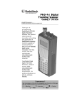


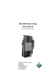
![RessqM, Enhanced Version of RESSQ [Javandel et al., 1984]](http://vs1.manualzilla.com/store/data/005674408_1-e8a4b9f66c80cdc83d847a710e5b4b1f-150x150.png)