1
HadCalc
manual
Michael Rauch
January 2006
Contents
1 Hadronic Cross Sections
1.1 Parton Model . . . . . . . . . . . .
1.2 Integrated Hadronic Cross Sections
1.3 Differential Hadronic Cross Sections
1.3.1 Invariant Mass . . . . . . .
1.3.2 Rapidity . . . . . . . . . . .
1.3.3 Transverse Momentum . . .
1.4 Cuts . . . . . . . . . . . . . . . . .
1.5 HadCalc . . . . . . . . . . . . . . .
.
.
.
.
.
.
.
.
.
.
.
.
.
.
.
.
.
.
.
.
.
.
.
.
.
.
.
.
.
.
.
.
.
.
.
.
.
.
.
.
.
.
.
.
.
.
.
.
.
.
.
.
.
.
.
.
.
.
.
.
.
.
.
.
.
.
.
.
.
.
.
.
.
.
.
.
.
.
.
.
.
.
.
.
.
.
.
.
.
.
.
.
.
.
.
.
.
.
.
.
.
.
.
.
.
.
.
.
.
.
.
.
.
.
.
.
.
.
.
.
.
.
.
.
.
.
.
.
1
1
2
3
3
4
5
6
10
2 Manual of the HadCalc Program
2.1 Prerequisites and Compilation . . . . .
2.1.1 Prerequisites . . . . . . . . . . .
2.1.2 Configuration and Compilation
2.2 Running the program . . . . . . . . . .
2.2.1 Physics parameters . . . . . . .
2.2.2 PDF parameters . . . . . . . .
2.2.3 Integration parameters . . . . .
2.2.4 Amplitude switches . . . . . . .
2.2.5 Input/Output options . . . . .
2.2.6 Amplitude calculation . . . . .
2.3 Allowed tokens in input files . . . . . .
2.4 Allowed variable names for outputstring
.
.
.
.
.
.
.
.
.
.
.
.
.
.
.
.
.
.
.
.
.
.
.
.
.
.
.
.
.
.
.
.
.
.
.
.
.
.
.
.
.
.
.
.
.
.
.
.
.
.
.
.
.
.
.
.
.
.
.
.
.
.
.
.
.
.
.
.
.
.
.
.
.
.
.
.
.
.
.
.
.
.
.
.
.
.
.
.
.
.
.
.
.
.
.
.
.
.
.
.
.
.
.
.
.
.
.
.
.
.
.
.
.
.
.
.
.
.
.
.
.
.
.
.
.
.
.
.
.
.
.
.
.
.
.
.
.
.
.
.
.
.
.
.
.
.
.
.
.
.
.
.
.
.
.
.
.
.
.
.
.
.
.
.
.
.
.
.
.
.
.
.
.
.
.
.
.
.
.
.
11
11
11
12
14
14
15
16
17
17
19
19
23
A Phase-space parametrization
A.1 Two-particle phase space . . . . . . . . . . . . . . . . . . . . . . .
A.2 Three-particle phase space . . . . . . . . . . . . . . . . . . . . . .
27
27
28
Bibliography
30
i
.
.
.
.
.
.
.
.
Chapter 1
Hadronic Cross Sections
The cross sections which are obtained by applying the Feynman rules contain,
amongst other particles, quarks and gluons. The leading interaction between
these particles is the strong interaction, which is described by quantum-chromo
dynamics (QCD). This theory possesses two characteristic properties: asymptotic
freedom [1] and confinement. Asymptotic freedom describes the behavior of the
theory at small distances. In this region the interaction is weak and the coupling
constant gets smaller with decreasing distance or, equivalently, with rising energy.
At large distances confinement appears, because the interaction becomes strong
and binds the particles tightly together. If the space between them becomes
even larger, it is energetically favorable to form new quark–anti-quark pairs. One
consequence of this behavior is that quarks and gluons cannot be observed as free
particles, but only as constituents of hadrons, i.e. mesons, which are quark–antiquark pairs, and baryons, which are states of three quarks or three anti-quarks.
An example for these hadrons are protons, which are the colliding particles at the
LHC. To make theoretical predictions it is necessary to relate the interactions at
the parton level to the interactions at the hadron level [2]. The basis for doing
this is the parton model [3], which will be described in the next section.
1.1
Parton Model
The parton model describes the inner structure of hadrons in hard collisions. It
starts from the assumption that every observable hadron consists of constituents,
the so-called partons, which can be identified as quarks and gluons. Experimental
evidence for this assumption comes from the observation of scaling [4] in deep
inelastic electron-proton-scattering. If the hadron carries some momentum P µ ,
the partons which take part in the partonic subprocess have momentum xP µ
with x ∈ [0, 1]. As normally the mass of the hadrons is small compared to their
kinetic energy one can assume P 2 = 0.
The interaction of an electron and a hadron or of two hadrons among each
1
2
Chapter 1. Hadronic Cross Sections
other can be split into two parts. Because of Lorentz contraction and time dilation
the interaction time of the two incoming particles in the laboratory frame is very
short. Therefore effectively a static hadron is seen. For the hard scattering
process interactions between partons of the same hadron need not be considered.
Also the process of hadronization after the interaction happens on time scales
which are much larger than the interaction itself.
From this the theorem of factorization [5] follows immediately. It states that
all diagrammatic contributions to the structure functions can be separated into a
product of two functions C and f , which depend on two mass scales µR and µF .
µR is the renormalization scale, µF is the so-called factorization scale and separates the long-distance from the short-distance effects. Slightly simplifying one
can say that every parton propagator which is off-shell by µF or more contributes
to C, while those which are below this value contribute to f .
1.2
Integrated Hadronic Cross Sections
The hard scattering process C therefore can be calculated in perturbation theory
by Feynman rules, using partons as incoming particles. It is independent of
long-distance effects and especially from the type of the colliding hadron.
The parton distribution function (PDF) fi/h (x, µF ) contains the long-distance
effects. It is independent of the underlying scattering process, but depends on µF
and the type of hadron h. It is normalized such that it can also be interpreted
as a probability density, namely the probability of finding the parton i in the
hadron h with a momentum xP µ . Its behavior as a function of the parameters is
determined by the Altarelli-Parisi integro-differential equations [6]. Its numerical
value, however, cannot be calculated a priori from the theory. At a single reference
point it must be determined by experiments.
Therewith one obtains the expression [2]
X Z 1 dL
σpp→f in+X =
dτ
σ̂mn→f in (τ S, αs (µR ))
(1.1)
dτ
τ0
{m,n}
for an integrated hadronic cross section with the parton luminosity
Z 1
dx
dL
1
=
·
dτ
x 1 + δmn
τ
τ
τ
, µF + fn/p (x, µF ) fm/p
, µF
.
(1.2)
· fm/p (x, µF ) fn/p
x
x
√
Here S denotes the hadronic center-of-mass energy, i.e. the one of the two
colliding protons, and σ̂mn→f in the partonic cross sections of the subprocesses,
where the two incoming partons m and n produce some final state, labeled f in.
The sum includes all possible parton combinations m and n where the order of
3
1.3. Differential Hadronic Cross Sections
appearance is not taken into account. The integration variable τ relates the par√
tonic and hadronic center-of-mass energies with each other. More specifically, τ
can be interpreted as the part of the hadronic center-of-mass energy which takes
part√in the
√ partonic subprocess, as the partonic center-of-mass energy is given
by ŝ = τ S. √
The lower limit of the integral τ0 is determined by the kinematic
configuration.
τ0 S is the minimal energy which is necessary to produce the
final state f in and therefore denotes the production threshold.
The formula given above is valid for processes with two or more particles in the
final state. For hadronic cross sections it is also possible to calculate integrated
cross sections for 2 → 1 processes. One first obtains for the partonic cross section
of the process mn → f
dσ̂mn→f =
π
2
0
0
0
√
|M
(mn
→
f
)
|
δ
p
+
p
−
p
f
i
m
n
f
4p0f ŝ|~pm |
.
(1.3)
Again m and n specify the incoming partons, f denotes the outgoing particle,
mf its mass, and p0i the energy of the respective particle i. p~m indicates the
three-momentum of particle m in the partonic center-of-mass system and Mf i is
the matrix element.
When convoluting with the parton distribution functions the single remaining δ-function in the partonic cross sections solves the τ integral in eq. (1.1)
analytically. Thus one obtains for the integrated hadronic cross section
X dL π
σpp→f =
|Mf i (mn → f ) |2 .
(1.4)
2
m
dτ τ = f 2mf S|~pm |
{m,n}
1.3
S
Differential Hadronic Cross Sections
Additionally one can define hadronic cross sections that are differential in one
or more parameters. For these parameters it is useful to take variables that are
either invariant under Lorentz transformations or at least have very simple transformation properties. In this thesis three differential hadronic cross sections are
presented which are also implemented in the HadCalc program that is described
below in section 1.5. They are cross sections differential with respect to the invariant mass of the final-state particles, the rapidity of one final-state particle
and, thirdly, the transverse momentum.
1.3.1
Invariant Mass
The first differential hadronic cross section is the one with respect to the invariant
mass of the final-state particles. The
mass of a process is equivalent to
√ invariant
√
the partonic center-of-mass energy ŝ ≡ τ S of the process or, in other words,
4
Chapter 1. Hadronic Cross Sections
the sum of the final-state momenta of the outgoing particles. The differential
cross section takes the form
√
ŝ X dL dσpp→f in
√
= 4π
σ̂mn→f in ,
(1.5)
S
dτ τ = ŝ
d ŝ
{m,n}
S
where f in again labeles a general final state.
1.3.2
Rapidity
The rapidity y of a particle is defined as
y = artanh
1 p0 + pz
pz
≡
ln
p0
2 p0 − pz
(1.6)
where pz = p~ · cθ denotes the fraction of the particle’s three-momentum p~ that
goes in the direction of the beam axis, labeled z. The mass of the particle will
later be referred to as m. Using the rapidity instead of directly taking the angle
θ between the particle and the beam axis possesses some advantages because the
rapidity of a particle has a few useful properties. Under a boost in the z-direction
to a frame with a velocity β, the rapidity transforms as y → y − artanh β. Thus
the shape of the rapidity distribution dσ
stays unchanged. More generally, the
dy
sum of two rapidities when the momenta point into the same direction is given by
the rapidity of the sum of the momenta, added via
the formula for the relativistic
p1 +p2
addition of velocities: y (p1 ) + y (p2 ) = y 1+p1 p2 . In experimental analyses often
a slightly different measure, the pseudo-rapidity η, is used. It is derived from the
standard rapidity by taking the limit of a vanishing mass of the particle and is
defined as
1 1 + cθ
η = ln
.
(1.7)
2 1 − cθ
In the HadCalc program both normal rapidity and pseudo-rapidity are implemented. As conversion between both variables can be performed by the simple
transformation
s
!
m2
tanh η
,
(1.8)
1− 2
y = artanh
p~ + m2
in the following only the shorter expressions for the standard rapidity are given.
The ones for pseudo-rapidity can then be deduced from them.
Using the above-mentioned definition of the rapidity the differential hadronic
cross section with respect to the rapidity for 2 → 2 processes then reads
Z 1
dσ
dL dσ̂ ∂cθ̂
dτ
=
.
(1.9)
dy
dτ dcθ̂ ∂y
τ0
5
1.3. Differential Hadronic Cross Sections
The momenta and masses given in the formulae always refer to the particle for
which the rapidity distribution is calculated. The angle cθ̂ between the particle
and the beam axis in the partonic center-of-mass system is fixed by the relation
s
1 x2
m2
(1.10)
cθ̂ = 1 + 2 tanh y + ln
2
τ
~p̂
where the second term in the argument of tanh originates from the boost from the
hadronic center-of-mass system, which is the laboratory frame, to the partonic
one, in which the partonic subprocess is calculated. This leads to
s
∂cθ̂
m2
1
= 1+ 2
.
(1.11)
2
2
∂y
~p̂ cosh y + 21 ln xτ
For processes with three or more particles in the final state the formula is
very similar. Additional phase-space integrals appear for the further particles
but otherwise eq. (1.9) stays unchanged. In the following equation the differential
cross section for a 2 → 3 process is given
Z
Z
Z
Z 1
∂cθ̂
dσ̂
dL
dσ
0
0
dτ
dk3 dk5 dη̂ 0
=
.
(1.12)
dy
dτ
dk3 dcθ̂ dk50 dη̂ ∂y
τ0
The parametrization of the three-particle phase space is described in appendix A.2.
1.3.3
Transverse Momentum
The last implemented differential hadronic
section is the one with respect
p 2 cross
2
to the transverse momentum pT = px + py of one of the final state particles.
For 2 → 2 processes it is defined as
Z 1
dL dσ̂ ∂cθ̂
dσ
dτ
=
(1.13)
dpT
dτ dcθ̂ ∂pT
τ̃0
with
∂cθ̂
1
=r
∂pT
2
~p̂ 4
− ~p̂
p2
(1.14)
T
which follows from
s
cθ̂± = ± 1 −
p2T
~p̂ 2
.
(1.15)
Here two possible solutions arise because of the sign ambiguity when taking the
square root. In principle both solutions have to be taken into account and added
6
Chapter 1. Hadronic Cross Sections
up unless they are excluded by other constraints as shown below. The lower limit
of the τ -integral τ̃0 must be adjusted such that sθ̂ is always inside its co-domain
[0; 1]
τ̃0 =
2
q
q
m2f1 + p2T + m2f2 + p2T
S
(1.16)
,
f1 and f2 denoting the two final state particles.
For 2 → 3 processes the extension to include the third final-state particle is
straightforward. The lower limit for τ in these processes is
τ˜0 =
q
2
q
2
m2f1 + p2T + (mf2 + mf3 ) + p2T
S
,
(1.17)
when the cross section is differential in the particle f1 . Therefore the expression
for the differential cross section reads
Z
Z
Z
Z 1
∂cθ̂
dσ̂
dL
dσ
0
0
dτ
dk3 dk5 dη̂ 0
=
.
(1.18)
0
dpT
dτ
dk3 dcθ̂ dk5 dη̂ ∂pT
τ˜0
1.4
Cuts
In order to improve the ratio of the signal-process cross section to that of the
background processes it can be useful to place appropriate cuts on the final-state
particles. Also experimental techniques used in the reconstruction of events like
jet-clustering algorithms can mandate the use of cuts in theoretical predictions,
so that the behavior of these techniques is emulated there.
In the HadCalc program cuts on three different properties of the final-state
particles are implemented [7]. The first two are cuts on the rapidity and the
transverse momentum of a particle. The definition of these two variables was
already presented in the previous section. The third one is a mutual property of
two particles, the jet separation ∆Rij , which is defined as
q
(1.19)
∆Rij = ∆yij2 + ∆φ2ij .
∆yij denotes the rapidity difference between the two particles i and j and ∆φij
the difference in the azimuthal angles of the two particles in the transverse plane.
Its main use are exclusive hadronic cross sections where final-state jets shall be
observed explicitly. It mimics the behavior of jet-clustering algorithms. There
two jets, which are separated by a jet separation below a certain limit, are seen in
the reconstruction as a single jet which has kinematic properties that are averaged
over the two final-state partons.
7
1.4. Cuts
For the first two cut parameters, rapidity and transverse momentum, it is
possible to translate these cuts into a limit on the integration parameters of
the phase space. The most general case is assumed here that cuts on both the
rapidity ycut and the transverse momentum pT cut of a particle shall be applied.
Using eq. (1.15) the transverse-momentum cut can be translated into a cut on cθ̂
and one obtains
s
s
2
p
pT 2cut
T
cut
<
c
<
≡ cmax
.
(1.20)
1
−
1
−
cmin
≡
−
θ̂
θ̂pT
θ̂pT
~p̂ 2
~p̂ 2
Likewise, the cut on the rapidity can also be turned into a cut on cθ̂ via eq. (1.10),
yielding
s
1 x2
m2
cθ̂ > 1 + 2 tanh −ycut + ln
≡ cmin
θ̂y
2
τ
~p̂
s
1 x2
m2
cθ̂ < 1 + 2 tanh ycut + ln
≡ cmax
.
θ̂y
2
τ
~p̂
To shorten the notation the abbreviation
v
u
2
u 1 − pT cut
u
~p̂ 2
r=t
2
1+ m
~2
(1.21)
(1.22)
p̂
is used in the following. Again the momenta and mass used in the equations all
refer to the particle whose phase space should be constrained.
Applying both cuts requires that the conditions on cθ̂ are all fulfilled simultaneously. This also restricts the integral on x which appears in the parton
luminosity given in eq. (1.2). In total the x-interval divides into five different
regions, which will be labeled by roman numbers. First the two cases where both
cuts cannot be fulfilled simultaneously, are considered, because the lower limit of
one cut lies above the upper limit of the other one:
Region I:
Region V:
cmin
θ̂pT
⇒
cmin
≥ cmax
θ̂y
θ̂p
⇒
cmax
θ̂y
≤
T
√
r
1−r
≡ xI
1+r
r
√ ycut 1 + r
x ≥ τe
≡ xV .
1−r
x≤
−ycut
τe
(1.23)
(1.24)
These two regions are excluded and the cross section vanishes there.
For specifying the other regions first two special cases are considered, where
the lower limits on cθ̂ and the upper limits, respectively, coincide. For these cases
8
Chapter 1. Hadronic Cross Sections
the according value of x is determined
cmin
θ̂y
cmin
θ̂pT
⇒
cmax
= cmax
θ̂y
θ̂p
⇒
=
T
√
r
1−r
≡ xmin
1+r
r
√
1+r
x = τ e−ycut
≡ xmax
1−r
x=
ycut
τe
(1.25)
.
(1.26)
Using these two definitions the other intermediate regions can be specified.
The ranges for cθ̂ which are deduced from these following regions specify the
allowed area where the cuts are fulfilled and therefore the cross section does not
vanish. The next two regions handle the cases where the limits on cθ̂ from rapidity
and transverse momentum overlap and one limit is given by the rapidity cut and
the other one by the transverse-momentum cut:
Region II:
⇒ xI < x < min(xmin , xmax )
< cθ̂ < cmax
≤ cmax
cmin
≤ cmin
θ̂y
θ̂p
θ̂y
θ̂p
T
T
(1.27)
Region IV:
≤ cmax
⇒
cmin
≤ cmin
< cθ̂ < cmax
θ̂p
θ̂y
θ̂p
θ̂y
T
T
max(xmin , xmax ) < x < xV
(1.28)
Finally the definition of the last region is the case whether one cut gives a
range on cθ̂ that completely lies inside the other one. Depending on which cut
this is, the limits on x are different:
Region III a):
≤ cmax
cmin
≤ cmin
< cθ̂ < cmax
θ̂y
θ̂p
θ̂p
θ̂y
⇒ xmin < x < xmax
cmin
θ̂y
⇒ xmax < x < xmin
T
T
Region III b):
≤
cmin
θ̂pT
< cθ̂ <
cmax
θ̂pT
≤
cmax
θ̂y
(1.29)
.
(1.30)
In addition to those regions the original constraint for x for a hadronic cross
section without cuts applies:
τ <x<1 .
(1.31)
Combining the result of all regions one can see that no holes in the integration over
x or cθ̂ appear and the final borders of the integration routine can be simplified
to
max(τ, xI ) < x < min(xV , 1)
(1.32)
) .
, cmax
) < cθ̂ < min(cmax
, cmin
max(cmin
θ̂y
θ̂p
θ̂y
θ̂p
(1.33)
and
T
T
.
9
1.4. Cuts
For a cross section which is differential with respect to the rapidity of a final
state particle the cut on the transverse momentum yields a restriction on cθ̂ in
the same way as in eq. (1.33)
< cθ̂ < cmax
cmin
θ̂p
θ̂p
(1.34)
.
T
T
The constraint on x must then be adjusted such that cθ̂ is always inside this
allowed interval, yielding
max(τ,
√
−y
τe
r
√
1−r
) < x < min( τ e−y
1+r
r
1+r
, 1) ,
1−r
(1.35)
which corresponds to eq. (1.32) where the rapidity cut ycut is replaced by its value
y given as an argument to the cross section.
Similarly, for cross sections that are differential in the transverse momentum
of a final-state particle a cut on the rapidity puts a further constraint on the
allowed interval for cθ̂ ± :
cmin
< cθ̂± < cmax
θ̂y
θ̂y
(1.36)
with
cmin
θ̂y
cmax
θ̂y
s
1 x2
m23
≡ 1 + 2 tanh −ycut + ln
2
τ
~p̂
s
1 x2
m23
.
≡ 1 + 2 tanh ycut + ln
2
τ
~p̂
(1.37)
(1.38)
Again this leads to a corresponding change in the limits of the x-integration which
are given by
max(τ,
√
−ycut
τe
r
√
1 − r̃
) < x < min( τ eycut
1 + r̃
r
1 + r̃
, 1)
1 − r̃
(1.39)
with
v
u
2
u 1 − p~T2
u
p̂
r̃ = t
m2
1 + ~ 23
.
(1.40)
p̂
This again corresponds to eqs. (1.32) and (1.22) where instead of the cut on
the transverse momentum pT cut its fixed value pT , which is an argument to the
differential cross section, is taken.
10
1.5
Chapter 1. Hadronic Cross Sections
HadCalc
For the numerical evaluation of the cross sections presented in the following chapters a program called HadCalc was developed to facilitate this task. It is based
on the established program packages FeynArts [8] and FormCalc [9, 10] which
are used to generate the partonic cross sections. The main task of HadCalc then
consists of the convolution with the PDFs that are taken from the PDFlib [11]
or LHAPDF [12] library packages that include PDF fits from various groups.
With this program it is possible to calculate both totally integrated and differential hadronic cross sections of processes with up to three particles in the final
state. The latter ones can be differential with respect to the partonic center-ofmass energy, or the rapidity or the transverse momentum of one of the outgoing
particles. Several cuts can be applied to the phase space. HadCalc operates
either in batch mode, where the parameters are read from a file and the cross
sections are written back to disk, allowing for easy post-processing with e.g. a
tool that generates plots. It can also be used in interactive mode where in- and
output are done via keyboard and screen and which allows the user for example
to tune the parameters most easily.
Chapter 2
Manual of the HadCalc Program
For the calculation of hadronic cross sections a computer code, called HadCalc,
was written (see chapter 1.5). In this appendix the manual of the program is
presented.
2.1
2.1.1
Prerequisites and Compilation
Prerequisites
The following programs are required for compiling and running HadCalc and
must be installed:
• a Fortran compiler compliant with the Fortran77 standard,
• a C compiler conforming to ANSI-C,
• GNU make,
• FormCalc 4 [9],
• one of the two following packages that include sets of parton distribution
functions from various groups
– PDFLIB (CERN Computer Program Library entry W5051) [11], or
– LHAPDF [12].
Additionally, support for the following two programs is integrated into HadCalc
• FeynHiggs 2.1beta or newer [13],
• Condor workload management system for compute-intensive jobs.
11
12
Chapter 2. Manual of the HadCalc Program
PDG flavor code Particle
0
gluon g
1
down quark d
2
up quark u
3
strange quark s
4
charm quark c
5
bottom quark b
6
top quark t
-1
down anti-quark d¯
-2
up anti-quark ū
-3
strange anti-quark s̄
-4
charm anti-quark c̄
-5
bottom anti-quark b̄
-6
top anti-quark t̄
Table 2.1: PDG flavor codes
2.1.2
Configuration and Compilation
First the partonic subprocess must be generated and prepared by following the
instructions in the FormCalc4 manual. Especially the definitions in process.h
have to be updated correctly as HadCalc relies on those. It is not necessary to
fill in correct MSSM parameters or tune integration parameters, however.
Then the distribution file HadCalc-0.5.tar.gz should be unpacked. As next
step change into its subdirectory and run configure from there. The following
configure options are mandatory:
--with-partonprocess=DIR This is the location of the FormCalcgenerated partonic output.
--with-processtype=mn
By this option the processtype is fixed,
specified by the number of incoming particles m and the number of outgoing particles n. Note that m and n form a single number, i.e. for a 2 → 2 process
one would write --with-processtype=22.
Currently, 2 → 1, 2 → 2 and 2 → 3 is
implemented and can be entered here.
--with-parton1=i
The type of the first parton is specified
by i, given as the PDG flavor code [14]
(see table 2.1).
--with-parton2=i
Similarly, this is the PDG flavor code for
the second parton.
2.1. Prerequisites and Compilation
13
Additionally the following options are recognized by configure and enable optional
features:
--enable-antiproton1
Hadron 1 is an anti-proton instead of a
proton.
--enable-antiproton2
Hadron 2 is an anti-proton instead of a
proton.
--with-condor[=DIR]
Link the final code with the Condor
workload management system libraries.
If the binary is not in the standard search
path of your shell, its location can be
specified with the optional DIR argument.
--with-feynhiggs[=DIR] Link the final code with the FeynHiggs library. This is mandatory if the
FormCalc option to compute the MSSMHiggs sector via FeynHiggs is chosen.
The optional DIR specifies the location
of the FeynHiggs library libFH.a, if it is
not in the standard search path of the
compiler.
--with-looptools=DIR
If LoopTools is not in the standard
search path of the compiler, its location
can be specified here.
--with-lhapdf[=DIR]
Use LHAPDF for the parton distribution
functions. If the LHAPDF library is not
in the standard search path, its location
can be given by the optional DIR argument. The PDF data is assumed to be
found at the same place.
--with-pdflib[=DIR]
Use PDFlib for the parton distribution
functions. If the PDFlib library is not in
the standard search path and the CERNlib environment variables $CERN and
$CERN LEVEL are not set, the DIR
argument designates where it can be
found.
Only one of the last two options can be given on the command line. If neither
--with-lhapdf nor --with-pdflib was given, configure first tries to find LHAPDF
and, if this fails, probes the existence of PDFlib.
After having run configure, a call to make compiles the program. When
it successfully finishes, a binary called HadCalc has been created in the current
path.
14
2.2
Chapter 2. Manual of the HadCalc Program
Running the program
The program is simply started by running ./HadCalc. It will then present a
menu which allows one to tune various settings and start the calculation of cross
sections. The following subsections describe the possible settings in detail. An
item is chosen by typing the number shown in brackets before the item and
pressing “Enter”. In every menu “(0)” exits the submenu or, for the top level
menu, quits the program. Invalid input is ignored and an error message is written
on the screen.
2.2.1
Physics parameters
This submenu sets the parameters of the MSSM and related things and is divided
in three further submenus.
MSSM parameters
Here all values which correspond to parameters of the MSSM are set.
First let us look at menu item 16. This decides whether the program should
use a common mass MSU SY in the sfermion sector, or if individual values for
the left-handed squarks and sleptons and the right-handed sups, sdowns and
selectrons are allowed. Depending on this flag either the MS* variables cannot
be set (because they are fixed at MSU SY ) or MSU SY itself cannot be set (because
it is irrevelant and not used in the computation). When choosing a common
SUSY mass scale, the settings in the MS* variables are retained and restored
when deselecting this option.
All other parameter settings can be in two states. They can either have a
fixed setting, then this value is used for all calculations. Or their value can be
running. In this case a lower and upper bound and the number of intermediate
intervals must be chosen. Then the computation of the cross section is done
(“intermediate intervals” + 1) times, with the value of the parameter increasing
from lower bound to upper bound1 . The distance between two values is equal for
the setting “linear” and exponentially increasing for the setting “logarithmic”,
i.e. the values are closer at the lower bound and they have equal distance again
when plotting them on a logarithmic scale. A behavior vice versa with values
closer at the upper bound can be easily achieved by exchanging lower and upper
bound. If more than one parameter is chosen to be running, the iteration loops
are nested, with the first parameter varying fastest.
1
Despite its name, the lower bound can be mathematically larger than the upper bound;
then the value of the parameter is decreasing.
2.2. Running the program
15
Kinematic parameters
In this menu all parameters are set which are related to kinematic variables of
the process.
The underlying parameter of items 3 and 4 depends on the type of process.
For processes with two particles in the final state, this is the angle θ between the
two outgoing particles, for those with three final particles, it denotes the energy
k50 of the fifth particle, which is the third final-state particle. The menu items 8,
12, 14 and 15, which refer to the fifth particle, are ignored for 2 → 2 processes
and cannot be changed.
The settings of the parameters are possible in the same way as already described in the previous item.
Scale parameters
This menu sets the renormalization and factorization scale of the process in the
same way as described above. A negative number for the renormalization scale
has a special meaning. Then the sum of the masses of the final-state particles
is taken, multiplied with the absolute value of the setting, and this number is
taken as the renormalization scale. Additionally it can be chosen that both
renormalization and factorization scale are always set to the same value.
Show ModelDigest (FormCalc)
Finally this choice invokes FormCalc’s ModelDigest function, which takes the parameters as an input and calculates the physical masses of the particles. Thereby
it applies lower bounds on the masses established by experiment and refuses the
calculation if these bounds are violated. The calculated cross section will also
be zero in that case. The FormCalc manual contains a more detailed explanation of this function. There it is also described how the check for the violation
of experimental bounds can be switched off by flipping a switch in FormCalc’s
process.h.
2.2.2
PDF parameters
The set used for the calculation of the parton distribution functions is chosen by
this submenu. The layout and choices presented depends on whether LHAPDF
or PDFlib is used. For PDFlib three numbers must be entered. The first denotes the type of parton distribution functions and is 1 for proton PDFs. The
second number specifies the respective group which has performed the fit to the
experimental data and the third number chooses a specific PDF set. When using
LHAPDF a string must be entered that directly specifies the filename of the PDF
set in the LHAPDF subdirectory.
16
Chapter 2. Manual of the HadCalc Program
2.2.3
Integration parameters
This submenu chooses the integration routine and sets its parameters. Currently
there are six integration routines available:
GAUSSKR
GAUSSAD
DCUHRE
VEGAS
SUAVE
DIVONNE
One-dimensional Gauss-Kronrod algorithm
One-dimensional adaptive Gauss algorithm
Multi-dimensional adaptive Gauss algorithm
Monte Carlo integration algorithm
Subregion adaptive Monte Carlo integration algorithm
Monte Carlo integration via stratified sampling
The last four algorithms are part of the CUBA library [15]. In the following only
a short description of the possible parameter settings is given. The technical
details of these algorithms and the precise impact of the variables are described
in the CUBA manual and shall not be repeated here.
The GAUSSKR and GAUSSAD algorithms can only handle one-dimensional
integrals. If multi-dimensional integrals are attempted to be computed, VEGAS
is used as a fallback. In contrast the DCUHRE and DIVONNE algorithms cannot handle one-dimensional integrals. There the GAUSSKR algorithm is used
instead. In both cases a warning is printed on the screen.
All integration routines share these two variables:
• relative error: the desired relative error
• absolute error: the desired absolute error
Additionally, the following variables are available for one or more of the routines.
Which ones these are is denoted in square brackets after the entry.
• maximum # of points: the maximum number of function evaluations used
[GAUSSAD, DCUHRE, VEGAS, SUAVE, DIVONNE]
• # of points for starting: the initial number of points per iteration [VEGAS]
• increase in # of points: the number of points the previous number is incremented for the next iteration [VEGAS]
• # of points for subdivision: the number of points used to sample a subdivision [SUAVE]
• flatness # for splits: the type of norm used to compute the fluctuation of
a sample [SUAVE]
• # of passes: the number of passes after which the partitioning phase terminates [DIVONNE]
2.2. Running the program
17
• key 1: determination of sampling in the partitioning phase [DIVONNE]
• key 2: determination of sampling in the final integration phase [DIVONNE]
• key 3: sets the strategy for the refinement phase [DIVONNE]
• maximum χ2 for subregion: the maximum χ2 value a single subregion is
allowed to have in the final integration phase [DIVONNE]
• minimum deviation for split: a bound which determines whether it is worthwhile to further examine a region that failed the χ2 test [DIVONNE]
2.2.4
Amplitude switches
This submenu sets the type of diagrams used for the computation and how the
cuts should be applied. The value of the cuts is set in the parameter section and
was already described there.
The first entry decides whether the tree-level and the one-loop result shall
be computed in one go or only one of them. Possible choices are “Tree only”,
“Tree+Loop” and “Loop only”. Which way is better depends on the concrete
circumstances and features of the problem. Computing both at the same time
might save computation time, but the integration routine has to optimize its
choices for both at the same time, which might lead to sub-optimal performance.
On the other hand it is not too likely that there are problematic regions in the
tree-level cross section which are no longer present in the one-loop computation,
so normally this procedure gives satisfactory results. If only one cross section is
computed, the value of the other one is set to zero.
The remaining entries decide if and how the cuts on rapidity, transverse momentum and jet separation should be applied. It is either possible to have the
particle, or a pair of particles in case of the jet separation, fulfill a cut, violate it
or ignore the cut altogether. Since HadCalc relies on FormCalc for the partonic
process and implementation details, for the cuts for particle three in the 2 → 2
case and particle five in the 2 → 3 case it cannot be chosen that the rapidity and
transverse momentum cut is violated, but they always have to be fulfilled. They
can, however, be switched off by setting the relevant entry in the parameters
section to zero.
2.2.5
Input/Output options
This submenu allows one to read in a set of parameters from a file and specify
where and how to write the calculation output.
To read in a set of parameters a parameter specification must have been
written into a file and this filename then has to be entered here. All possible
variables which can be set in such a file are given in section 2.3. There are three
18
Chapter 2. Manual of the HadCalc Program
basic types of variables. Those which specify a parameter can either take four
comma-separated values that are the lower and upper bound, the behavior with
respect to increments, i.e. linear or logarithmic, and the number of intermediate
intervals, or a single number denoting its fixed value. The ones of type boolean
turn on a certain switch and take no arguments. All remaining ones take a single
argument and the variable is assigned to this parameter.
In the following also a formal definition of the parsing rules is given:
• The file is read line by line.
• White space at the beginning of a line is ignored.
• Empty lines are ignored.
• Lines starting with the character “#” (after optional white space) are comment lines and ignored.
• The first token which is separated by white space from the rest of the line
is extracted. This token has to be a token from the list of valid tokens in
section 2.3.
• If the token type is boolean, its associated parameter is set.
• If the token type is integer, an attempt to read an integer value is made
and if it succeeds, this is assigned to the associated parameter.
• If the token type is double, an attempt to read a double precision floatingpoint number is made and if it succeeds, this is assigned to the associated
parameter.
• If the token type is string, the second token is assigned to the associated
parameter.
• If the token type is parameter, the following actions happen:
– An attempt to read four comma-separated double precision floatingpoint numbers is made.
– If this attempt succeeds, the four numbers are assigned to lower bound,
upper bound, log and number of intermediate intervals of the parameter. log means linear increase if this variable is zero and exponential
one otherwise.
– If this does not succeed, an attempt to read a single double precision
floating point number is made.
– If this succeeds, this number is the constant value of the parameter.
– If this also does not succeed, the line is flagged as not parsable.
2.3. Allowed tokens in input files
19
• For lines not parsable by the rules above a warning message is printed and
their content is ignored.
Furthermore some integration routines offer the possibility to write intermediate results or progress report to the screen. This is turned on with Verbose
integration output. For hadronic cross sections this also enables writing PDFlib
statistics on the screen at the end of the calculation.
Finally one can choose whether the calculation results will be written to the
screen or into a file. In the latter case the variable outputstring describes which
elements should be written to the output file. The form of this variable together
with the valid tokens is described in section 2.4. The output-file format starts with
a “#”-quoted header with a file identification and the content of outputstring.
Then, each on a line by itself, for every scanned parameter point the values
defined in outputstring are written, separated from each other by a space.
2.2.6
Amplitude calculation
This submenu finally allows one to choose the cross section one wants to compute
and does the calculation. During the following integration the process may be
interrupted with “Ctrl-C”, after which it aborts the current calculation and jumps
back into the main menu. Due to restrictions imposed by Condor this feature
is not available if HadCalc was configured with the option --with-condor. Here
pressing “Ctrl-C” aborts the whole HadCalc program.
2.3
Allowed tokens in input files
The following list shows all token names that may appear in an input file together
with its associated type. The tokens are not case-sensitive. Thereby parameter
means that the variable can either be followed by four comma-separated values
that denote the lower and upper bound, whether the increase is linear or logarithmic, and the number of intermediate intervals, or a single number that is the
fixed value of this parameter. boolean means that a specific behavior is switched
on. There is a corresponding separate token that switches the same behavior off
again. double and integer tokens take a single double-precision or integer value,
respectively, as input. string assigns the remainder of the line to the parameter.
Finally preselected takes special values as an argument. The possible choices
for each of these ones were discussed during the description of the menus given
in section 2.2. Any settings referring to particle 5 are relevant only for 2 → 3
processes and will be silently ignored otherwise.
20
Chapter 2. Manual of the HadCalc Program
token
MA0
TB
: type
: parameter
: parameter
MUE
MSusy
MSQ
: parameter
: parameter
: parameter
MSU
: parameter
MSD
: parameter
MSL
: parameter
MSE
: parameter
At
: parameter
Ab
: parameter
A tau
: parameter
M1
M2
MGl
SQRTS
:
:
:
:
SQRTSHAT
: parameter
THETA
2
THETACUT
parameter
parameter
parameter
parameter
: parameter
2
: parameter
K50 3
K50CUT
: parameter
: parameter
PTRANS 3
PTRANS3CUT
: parameter
: parameter
PTRANS4CUT
: parameter
2
only for 2 → 2 processes
description
mass of the CP-odd Higgs boson
ratio of the Higgs vacuum expectation values
µ parameter in the Higgs sector
common SUSY mass scale
mass parameter of the left-handed
squarks
mass parameter of the right-handed
sup-like squarks
mass parameter of the right-handed
sdown-like squarks
mass parameter of the left-handed
sleptons
mass parameter of the right-handed
selectron-like sleptons
trilinear coupling of the sup-like
squarks
trilinear coupling of the sdown-like
squarks
trilinear coupling of the selectronlike sleptons
U(1)Y gaugino mass
SU(2)L gaugino mass
SU(3)C gaugino mass
square root of the hadronic center
of mass energy
square root of the partonic center of
mass energy
angle between the two outgoing
particles (in degrees) 3
cut on the angle between the two
outgoing particles (in degrees)
energy of the third outgoing particle
cut on the energy of the third outgoing particle
transverse momentum
cut on the transverse momentum of
particle 3
cut on the transverse momentum of
particle 4
2.3. Allowed tokens in input files
token
PTRANS5CUT
: type
: parameter
RAPID 3
RAPID3CUT
RAPID4CUT
RAPID5CUT
DELTAR34CUT
:
:
:
:
:
DELTAR35CUT
: parameter
DELTAR45CUT
: parameter
RENSCALE
:
FACTSCALE
:
CommonSUSYMassScale :
NoCommonSUSYMassScale :
CommonRenFactScale
parameter
parameter
parameter
parameter
parameter
parameter
parameter
boolean
boolean
: boolean
NoCommonRenFactScale : boolean
AMPLITUDE
: preselected
Ptrans3>cut
: boolean
Ptrans3<cut
: boolean
Ptrans3nocut
: boolean
Rapid3>cut
: boolean
Rapid3<cut
: boolean
Rapid3nocut
: boolean
Ptrans4>cut
: boolean
3
only for differential cross sections
21
description
cut on the transverse momentum of
particle 5
rapidity
cut on the rapidity of particle 3
cut on the rapidity of particle 4
cut on the rapidity of particle 5
cut on the distance between particles 3 and 4
cut on the distance between particles 3 and 5
cut on the distance between particles 4 and 5
renormalization scale
factorization scale
choose a common SUSY mass scale
do not choose a common SUSY
mass scale
choose a common remormalization
and factorization scale
do not choose a common remormalization and factorization scale
choose which amplitude(s) to calculate
require the transverse momentum
of particle 3 to be larger than the
cut
require the transverse momentum
of particle 3 to be smaller than the
cut
disable cut on the transverse momentum of particle 3
require the rapidity of particle 3 to
be larger than the cut
require the rapidity of particle 3 to
be smaller than the cut
disable cut on the rapidity of particle 3
require the transverse momentum
of particle 4 to be larger than the
cut
22
Chapter 2. Manual of the HadCalc Program
token
Ptrans4<cut
: type
: boolean
Ptrans4nocut
: boolean
Rapid4>cut
: boolean
Rapid4<cut
: boolean
Rapid4nocut
: boolean
DeltaR34>cut
: boolean
DeltaR34<cut
: boolean
DeltaR34nocut
: boolean
DeltaR35>cut
: boolean
DeltaR35<cut
: boolean
DeltaR35nocut
: boolean
DeltaR45>cut
: boolean
DeltaR45<cut
: boolean
DeltaR45nocut
: boolean
INTMETHOD
EPSABS
EPSREL
MAXPTS
VSTARTPTS
VINCREASE
SNNEW
:
:
:
:
:
:
:
preselected
double
double
integer
integer
integer
integer
description
require the transverse momentum
of particle 4 to be smaller than the
cut
disable cut on the transverse momentum of particle 4
require the rapidity of particle 4 to
be larger than the cut
require the rapidity of particle 4 to
be smaller than the cut
disable cut on the rapidity of particle 4
require the jet separation between
particles 3 and 4 to be larger than
the cut
require the jet separation between
particles 3 and 4 to be smaller than
the cut
disable the cut on the jet separation
between particles 3 and 4
require the jet separation between
particles 3 and 5 to be larger than
the cut
require the jet separation between
particles 3 and 5 to be smaller than
the cut
disable the cut on the jet separation
between particles 3 and 5
require the jet separation between
particles 4 and 5 to be larger than
the cut
require the jet separation between
particles 4 and 5 to be smaller than
the cut
disable the cut on the jet separation
between particles 4 and 5
choose the integration routine
absolute integration error
relative integration error
maximum number of points
number of points for starting
increase in number of points
number of points for subdivision
2.4. Allowed variable names for outputstring
token
SFLATNESS
MAXDPASS
: type
: integer
: integer
DKEY1
DKEY2
DKEY3
DBORDER
MAXDCHISQ
MINDDEV
VERBOSITY
PDFTYPE
PDFGROUP
PDFSET
PDFPATH
:
:
:
:
:
:
:
:
:
:
:
integer
integer
integer
double
double
double
integer
double
double
double
string
PDFNAME
ScreenOutput
OUTPUTFILE
OUTPUTSTRING
:
:
:
:
string
boolean
string
string
2.4
23
description
flatness number for splits
number of passes in partitioning
phase
Divonne key 1
Divonne key 2
Divonne key 3
border of the integration region
maximum χ2 for subregion
minimum deviation for split
verbosity of integration output
type of the PDF [PDFlib]
group of the PDF [PDFlib]
set of the PDF [PDFlib]
path where the PDF files are
[LHAPDF]
name of the PDF [LHAPDF]
print output on the screen
print output into file
parameters to print in output (see
section 2.4)
Allowed variable names for outputstring
The following list shows all variable names that may appear in outputstring. The
individual entries are separated from each other by spaces. Variables with the
dimension of a mass are output in GeV. Note that these names are case-sensitive.
Name
MA0
TB
MUE
MSusy
MSQ
MSU
:
:
:
:
:
:
:
MSD
:
MSL
MSE
:
:
At
:
Parameter description
m A0
mass of the CP-odd Higgs boson
tan β
ratio of the Higgs vacuum expectation values
µ
µ parameter in the Higgs sector
mSU SY
common SUSY mass scale
mq̃
mass parameter of the left-handed squarks
mũ
mass parameter of the right-handed sup-like
squarks
md˜
mass parameter of the right-handed sdown-like
squarks
ml̃
mass parameter of the left-handed sleptons
mẽ
mass parameter of the right-handed selectron-like
sleptons
At
trilinear coupling of the sup-like squarks
24
Chapter 2. Manual of the HadCalc Program
Name
Ab
A tau
M1
M2
MGl
SQRTS 4
SQRTSHAT
THETA 6
THETACUT
5
6
:
:
:
:
:
:
:
:
:
:
K50 7
:
7
:
K50CUT
PTRANS
:
PTRANS3CUT :
PTRANS4CUT :
PTRANS5CUT :
RAPID
:
RAPID3CUT :
RAPID4CUT :
RAPID5CUT :
DELTAR34CUT :
DELTAR35CUT :
DELTAR45CUT :
RENSCALE
:
FACTSCALE :
Mh0
:
MH0
:
MHpm
:
MCha(1)
:
MCha(2)
:
MNeu(1)
:
MNeu(2)
:
MNeu(3)
:
MNeu(4)
:
MGl
:
MSn(1)
:
4
Parameter description
Ab
trilinear coupling of the sdown-like squarks
Aτ
trilinear coupling of the selectron-like sleptons
M1
U(1)Y gaugino mass
M2
SU(2)L gaugino mass
m
gluino
mass
√g̃
square root of the hadronic center-of-mass energy
√S
ŝ
square root of the partonic center-of-mass energy
θ
angle between the two outgoing particles (in degrees)
θcut
cut on the angle between the two outgoing particles
(in degrees)
k50
energy of the third outgoing particle
cut on the energy of the third outgoing particle
k50 cut
ptrans
transverse momentum
cut on the transverse momentum of particle 3
p3transcut
4
ptrans cut
cut on the transverse momentum of particle 4
cut on the transverse momentum of particle 5
p5transcut
η
rapidity
3
ηcut
cut on the rapidity of particle 3
4
ηcut
cut on the rapidity of particle 4
5
ηcut
cut on the rapidity of particle 5
∆R34 cut
cut on the distance between particles 3 and 4
∆R35 cut
cut on the distance between particles 3 and 5
45
∆R cut
cut on the distance between particles 4 and 5
µR
renormalization scale
µF
factorization scale
mass of the lighter CP-even Higgs boson
mh0
mass of the heavier CP-even Higgs boson
mH 0
mH ±
mass of the charged Higgs boson
m χ1
mass of the lighter chargino
m χ2
mass of the heavier chargino
mχ01
mass of the lightest neutralino
mχ02
mass of the second-lightest neutralino
mχ03
mass of the second-heaviest neutralino
mχ04
mass of the heaviest neutralino
mg̃
mass of the gluino
mν̃e
mass of the electron sneutrino
only relevant for the computation of hadronic cross sections
only relevant for the computation of partonic cross sections and differential hadronic cross
section with respect to invariant mass
6
only for 2 → 2 processes
7
only for 2 → 3 processes
5
2.4. Allowed variable names for outputstring
Name
MSn(2)
MSn(3)
MSl(1)
MSl(2)
MSl(3)
MSL(1)
MSL(2)
MSL(3)
MSu(1)
MSu(2)
MSu(3)
MSU(1)
MSU(2)
MSU(3)
MSd(1)
MSd(2)
MSd(3)
MSD(1)
MSD(2)
MSD(3)
TREE
LOOP
TREEERR
LOOPERR
TREEPROB
:
:
:
:
:
:
:
:
:
:
:
:
:
:
:
:
:
:
:
:
:
:
:
:
:
:
LOOPPROB
:
NREGIONS8
NEVAL8
FAIL8
:
:
:
8
25
Parameter description
mν̃µ
mass of the muon sneutrino
mν̃τ
mass of the tau sneutrino
mẽ1
mass of the lighter selectron
mµ̃1
mass of the lighter smuon
mτ̃1
mass of the lighter stau
mẽ2
mass of the heavier selectron
mµ̃2
mass of the heavier smuon
mτ̃2
mass of the heavier stau
mũ1
mass of the lighter sup
mc̃1
mass of the lighter scharm
mt̃1
mass of the lighter stop
mũ2
mass of the heavier sup
mc̃2
mass of the heavier scharm
mt̃2
mass of the heavier stop
md˜1
mass of the lighter sdown
ms̃1
mass of the lighter sstrange
mb̃1
mass of the lighter sbottom
md˜2
mass of the heavier sdown
ms̃2
mass of the heavier sstrange
mb̃2
mass of the heavier sbottom
σ0
tree-level cross section
σ1
one-loop cross section
σ(σ0 )
integration error of the tree-level cross section
σ(σ1 )
integration error of the one-loop cross section
χ2 (σ(σ0 )) probability of the integration error of the tree-level
cross section
2
χ (σ(σ1 )) probability of the integration error of the one-loop
cross section
number of regions used for integration
number of function evaluations used for integration
a non-zero value indicates that the desired accuracy
could not be reached
only relevant for some integration routines
Appendix A
Phase-space parametrization
In this appendix the parametrization of the phase space for 2 → 2 and 2 → 3
processes, as it was used for the calculations of this thesis, is presented. It
is the same parametrization which is also used in FormCalc [9, 10, 16]. The
parametrization is performed in the center-of-mass system of the two incoming
√
particles, which define the beam axis and carry a center-of-mass energy of s.
For each final-state particle an integral over its three-momentum ~k occurs in the
0
calculation of integrated cross
q sections. The energy k of the particle is fixed by
the on-shell condition k 0 = |~k|2 + m2 , where m denotes the mass of the particle.
Four of these integrals are eliminated by global energy-momentum conservation.
In the following sections the parametrizations of the two- and three-particle phase
space are shown.
A.1
Two-particle phase space
With two particles in the final state, labeled by the subscripts 3 and 4 in the
following, the phase-space integral can be written in terms of two angles. They
are the azimuth angle φ and the polar angle θ with respect to the beam axis.
Because of rotational invariance around the beam axis the integration over φ is
trivial and amounts to a factor of 2π. So the integral over the two-particle phase
space is given by
Z
Z 1
1 |~k3 |
√
,
(A.1)
dcθ
dΓ2 =
8π s
−1
where
s2 + m43 + m24 − 2m23 s − 2m24 s − 2m23 m24
|~k3 |2 = |~k4 |2 =
(A.2)
4s
denotes the squared absolute value of the three-momentum
of the final-state
√
particles, m3 and m4 are their respective masses, and s specifies the center-ofmass energy of the incoming particles.
27
28
Appendix A. Phase-space parametrization
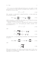
~k3
η̂
~k5
ξ
θ
~k2
~k1
~k4
y
x
z
Figure A.1: Graphical representation of the variables used in the parametrization
of the 2 → 3 phase space. The figure is taken from ref. [16].
A.2
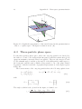
Three-particle phase space
For the three-particle phase space, where the outgoing particles are labeled by
the indices 3, 4 and 5, five independent integration variables remain after global
energy-momentum conservation has been applied. They are the energies k30 and
k50 , the azimuth angle φ and the polar angle θ of the fifth particle with respect to
the beam axis, and the angle η̂ which rotates particle 3 out of the plane defined
by particle 5 and the beam axis. A graphical representation of the angles is given
in Fig. A.1.
The four-momenta of the outgoing particles have the following explicit form
√
k3 = (k30 , |~k3 |~e3 )
k4 = ( s − k30 − k50 , −~k3 − ~k5 )
k5 = (k 0 , |~k5 |~e5 ) ,
(A.3)
5
with
cθ cη̂ sξ + sθ cξ
sη̂ sξ
~e3 =
cθ cξ − sθ cη̂ sξ
sθ
~e5 = 0
cθ
The angle θ, which is also plotted in the figure, is defined over
√
( s − k30 − k50 )2 − m24 − |~k3 |2 − |~k5 |2
.
cθ =
2|~k3 ||~k5 |
.
(A.4)
(A.5)
29
A.2. Three-particle phase space
√
mi again denotes the mass of the respective particle i and s is the center-of-mass
energy of the initial-state particles. Due to axial symmetry the trivial integration
over φ can be carried out immediately and yields a factor of 2π.
Then the parametrization of the three-particle phase space takes the following
form
Z (k30 )max
Z 2pi
Z 1
Z
Z (k50 )max
1
0
0
,
(A.6)
dk5
dk3
dη̂
dcθ
dΓ3 =
64π 3
(k30 )min
m5
0
−1
where the integration limits are given by
√
s (m3 + m4 )2 − m25
0 max
√
(k5 )
=
−
2
2 s
(A.7)
and
(k30 )max,min
q
1
2
2
~
=
σ(τ + m+ m− ) ± |k5 | (τ − m+ )(τ − m− )
2τ
,
(A.8)
using
σ=
√
s − k50
τ = σ 2 − |~k5 |2
m± = m3 ± m4
.
(A.9)
Bibliography
[1] D. J. Gross and F. Wilczek. Phys. Rev. Lett., 30:1343–1346, 1973; H. D.
Politzer. Phys. Rev. Lett., 30:1346–1349, 1973.
[2] R. Brock et al. Rev. Mod. Phys., 67:157–248, 1995; R. Brock et al. Handbook
of perturbative QCD; Version 1.1: September 1994, FERMILAB-PUB-94316, 1994.
[3] J. D. Bjorken and E. A. Paschos. Phys. Rev., 185:1975–1982, 1969; R. P.
Feynman. Phys. Rev. Lett., 23:1415–1417, 1969.
[4] E. D. Bloom et al. Phys. Rev. Lett., 23:930–934, 1969; M. Breidenbach et al.
Phys. Rev. Lett., 23:935–939, 1969; J. I. Friedman and H. W. Kendall. Ann.
Rev. Nucl. Part. Sci., 22:203–254, 1972.
[5] J. C. Collins, D. E. Soper, and G. Sterman. Adv. Ser. Direct. High Energy
Phys., 5:1–91, 1988.
[6] G. Altarelli and G. Parisi. Nucl. Phys., B126:298, 1977.
[7] C. Meier. γZ-Produktion in P-P-Kollisionen mit elektroschwachen 1Schleifen-Korrekturen. Diplom thesis, Universität Karlsruhe, July 2001.
[8] J. Kublbeck, M. Bohm, and A. Denner. Comput. Phys. Commun., 60:165–
180, 1990; T. Hahn. Comput. Phys. Commun., 140:418–431, 2001; T. Hahn
and C. Schappacher. Comput. Phys. Commun., 143:54–68, 2002.
[9] T. Hahn and M. Perez-Victoria. Comput. Phys. Commun., 118:153–165,
1999.
[10] T. Hahn. New developments in FormCalc 4.1, hep-ph/0506201, 2005.
[11] H. Plothow-Besch. PDFLIB - User’s Manual Version 8.04. CERN-ETT/TT
2000.04.17.
[12] W. Giele and M. Whalley. LHAPDF version 4 Users Guide, April 2002.
http://durpdg.dur.ac.uk/lhapdf/manual.htm.
31
32
Bibliography
[13] S. Heinemeyer, W. Hollik, and G. Weiglein. Comput. Phys. Commun.,
124:76–89, 2000.
[14] S. Eidelman et al. Phys. Lett., B592:1, 2004.
[15] T. Hahn. Comput. Phys. Commun., 168:78–95, 2005.
[16] T.
Hahn.
FormCalc 4 User’s Guide,
http://www.feynarts.de/formcalc/FC4Guide.ps.gz.
March
2005.