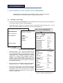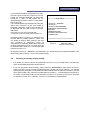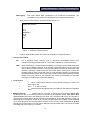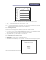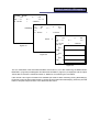
1
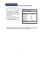
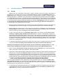
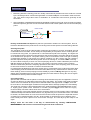
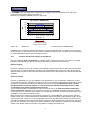
Operator’s Manual
CONTENTS
1. Specifications
1.1
PID analyzer
1.2
IR analyzer
1.3 Applications
2. Instrument Description
2.1 Basic Controls
2.1.1
Display panel
2.1.2
Handle Control
2.2 The front of the instrument
3. Start ECOPROBE 5
4. Main Menu
5. How to enter a locality using Locality Management
5.1 Entering a new locality
5.2 Selecting an already existing locality
5.3 System Configuration File
6. How to start measurement using Locality1, Locality 2
6.1 Standard Grid
6.1.1
Measurement Mode
6.1.2
Measurement
6.1.3
Finishing measuring
6.1.4
Repeating the last measured point
6.1.5
Data Logging – Standard Grid
6.2 GPS logging
6.2.1
About Global Positioning
6.2.2
GPS and Ecoprobe 5
6.2.3
Measurement Mode
7. Continuous measurement
8. Monitor
8.1 How to enter and measure a Monitoring station
9. Communication
10. System Configuration
11. Calibration
11.1 PID unit
11.2 IR unit
11.3 Ecoprobe 5 Calibration procedure
12. The field survey
12.1 General
12.2 How to interpret a photoionization breakdown phenomenon
of the PID unit
12.3 Relative and absolute outputs of the PID unit
13. General
13.1 Power Supply
13.2 Warranty
13.3 Troubleshooting
13.4 Important Notes
1
2
2
3
3
5
5
5
5
5
6
7
8
8
9
10
14
14
14
14
15
15
16
18
18
18
20
22
23
23
25
26
27
27
28
28
35
35
37
38
40
40
40
40
40
Specifications
1.
SPECIFICATIONS
Ecoprobe 5 introduces a new level of flexibility, convenience, and quality to in-situ detection and analysis
of VOC’s and other contaminant indicators. Cost effective, definitive soil contaminant surveys which provide
an unprecedented breadth of high precision data result from its combination of PID and IR detectors
complemented by temperature and pressure data. A new dimension in detection is provided by the
simultaneous measurement of total soil gas / vapor concentration (PID detector) together with four channel
selective analyses for methane, carbon dioxide, oxygen, and petroleum hydrocarbons (IR detector).
1.1
PID analyzer
Characteristics
• Detection limit 0.1 ppb (0.0001ppm)
• ppb resolution, 0.1 ppb zero stability
• calibration for quantitative vapour phase determination for over 200 compounds included zero response
for methane ( methane measured separately by IR unit)
• large dynamic range (0.1 ppb to 4000 ppm), fast response (0.5 sec)
• ion lamp 10.2 eV (other energy levels are optional)
• STANDARD mode with ppm or mg/m3 output or HISENS mode with ppb or mg/m3 output
PID unit measures total concentration of volatile organic compounds (VOC) and other toxic gases
including chlorinated hydrocarbons, selectively excluding methane from the total sum.
Relative outputs
Ecoprobe 5 enables you to map a relative concentration cloud, identifies the contaminant sources, paths
and the range of contaminated area. Measuring by means of Ecoprobe 5 is simple, fast and cheap and
eliminates the principle of redundant and expensive analysis of the spectrally known and almost identical
samples.
Absolute outputs
PID unit is calibrated only for one calibration gas –Isobuthylene. The instrument’s responses to other
compounds are different. Calibration procedure, however, automatically calibrates the instrument for about
200 specific compounds (see table of measured compounds in Figure 35).
This feature is used in cases when composition of the contaminant is known and absolute results
of soil gas/vapour concentration are required. Choose the compound which is chemically equal or very
close to the contaminant and select it in the System Configuration File of the locality (described later). Then
the output can give quantitative concentration of vapour phase (For further details see Chapter 12.3).
Nevertheless, the operator should bear in mind that Ecoprobe 5 is neither a spectral analyzer nor
a spectral-selective detector.
Spectral characteristic of Ecoprobe 5 analytical unit is equal to the characteristics of the laboratory gas
chromatograph evaluating unit (if the lamp of equal energy is used). This means that spectral responses
to all the spectral components of Ecooprobe 5 and laboratory gas chromatograph are equal which brings
very close results between the in-situ total measurement and selective laboratory analysis of samples.
Photoionisation breakdown
Generally speaking, photoionisation process has its physical limit. For a concentration higher than certain
value the ionization process will breakdown. Further increase of concentration may even lead to the decay
of output. The average value of photoionisation breakdown limit is around 4000 ppm and varies for different
spectral compounds.
To indicate this phenomenon by means of the inner instrument software is not entirely clear and it is not
common for this type of instruments.
2
Specifications
RS DYNAMICS worked on a technique of photoionization breakdown indication with following results:
Ecoprobe 5 indicates the concentration exceeding breakdown limit by the message “over”displayed on the
instrument screen but this message is not displayed in all cases. Depending on different conditions
(particular compounds, the speed of photoionisation breakdown process, amount of concentration..) the
output may also show a low “breakdown” value (hundreds of ppm) for concentration higher than
photoionisation breakdown limit. Above mentioned facts must be considered in interpretation and are valid
for STANDARD mode. (see Chapter 12 – The field survey).
In case of HIGH SENSITIVE mode, the measured limit is 100 ppm. Higher values of concentration are
almost always indicated by the message “over”displayed on the instrument screen.
If hydrocarbons are presented in the contamination, consequent continuity between PID (in Standard
mode) and IR unit outputs can be observed after photoionisation breakdown of the PID unit.
If the contamination consists of other compounds (no hydrocarbons), there is no response of IR unit.
1.2
IR analyzer
Infra-red analyzer provides selective detection of methane, petroleum hydrocarbons and carbon dioxide.
Characteristics
• Four independent channels features following ranges with ppm resolution:
• Methane 0 – 500 000 ppm, detection limit 20 ppm
• Petroleum Hydrocarbons 0- 500 000 ppm (including Methane), detection limit 20 ppm
• Carbon Dioxide 0 – 500 000 ppm, detection limit 20 ppm
• Reference channel
• ppm or mg/m3 output
1.3
Applications
With the very high sensitivity of the PID, this instrument has capability that reaches well beyond the standard
soil vapour survey. Effectiveness in the detection and monitoring of contaminant spills and plume migration
is substantially enhanced by the incorporation of ancillary data. The remarkable zero stability, combined
with no response to methane, provides a detection capability undiminished by natural hydrocarbon
occurrence, ensuring the application of optimum sensitivity levels. UST and pipeline leakage detection and
localization are further extensions of the soil vapour applications, as is also the tracking of contamination
from agricultural waste. Less obvious applications are to be found in the detection and monitoring of organic
toxins in industrial applications. Minute traces of gas can be an indication of approaching breakdown of a
shaft seal or packing in a process vessel with externally driven components. Real time continuous display
mode makes localization of leakage with pinpoint accuracy a reality. Further applications incorporating the
IR and temperature detection are found in the in-situ monitoring of bio-remediation, where bacteria will
consume oxygen, and generate heat along with methane and carbon dioxide. Routine periodic repetition
of sampling at fixed locations can track both the progress and health or effectiveness of the process, since
the results provide a clear indication of bacterial activity as well as contaminant concentration.
Usefulness in brief:
• Detection, delineation & monitoring of hydrocarbon and other organic contamination of soils & water
table from fuel spills; air pollution monitoring (PID)
• Waste dumps UST leakage
• Pipe-line leakage & agricultural waste
• Monitoring of plume migration
• Monitoring of in-situ bio-remediation processes
• Detection and monitoring of gaseous toxins in industrial plants and agricultural applications.
3
Instrument Description
All the basic controls necessary for Ecoprobe 5's operations are described bellow. This user-friendly, easyto-operate system allows the operator to select the optimal settings for data gathering. Maximum benefit
is derived from Ecoprobe 5 by following the instructions systematically.
2.
INSTRUMENT DESCRIPTION
2.1
BASIC CONTROLS
2.1.1
Display panel -- four keys arranged in two islands (Figure 1)
ESC
Terminates operations and returns to the Main
Menu.
Starts a selected procedure.
Switches the instrument on/off.
While holding down the key, ? /? is used to
switch the screen back light on/off; ? /? is used
to change the screen contrast.
RUN
ON/OFF
LIGHT
2.1.2
Handle control -- four arrowed keys (Figure 1)
These are multi-functional switches and their actual operation or
function depends on the specific menu displayed.
Figure 1:
? /?
(Up/Down)
?
(Left)
?
(Right)
Moves the cursor up/down through a
menu.
Escapes from a current menu to return
to the previous level and saves a
selected option.
Selects an option from a menu, or initiates
a procedure/operation.
Display panel and handle controls
C
2.2
THE FRONT OF THE INSTRUMENT
(Figure 2)
(A)
Multifunctional connector for the charger, PC, GPS
receiver, probe thermometer and alternative power
sources like solar batteries or a car charging cable.
(B)
Gas inlet
(C)
Gas outlet
A
Figure 2:
4
The front
instrument
of
the
B
Start Ecoprobe 5
3.
START ECOPROBE 5
By pressing the ON/OFF key on the display panel, the instrument will boot up in about two seconds and
display the Welcome Menu (Figure 3).
RS DYNAMICS
ECOPROBE 5
Version # 990112
TIME
DATE
Pressure: 1009 mBarr
Figure 3:
Welcome Menu
Press any arrow on the handle control to open the Main Menu
5
Main Menu
4.
MAIN MENU
Brief explanation
LOCALITY 1 (or 2)
Measuring mode;
starts measurement of the locality.
************ MAIN MENU ***************
LOCALITY MANAGEMENT
Configurates a new
locality, already measured localities and monitoring
stations and deletes localities.
CONTINUOUS MEASUREMENT Allows continuous
operation without any data being logged.
MONITOR
Enables automatic monitoring of
contamination at a predetermined sampling rate.
COMMUNICATION
Enables transferring data from
Ecoprobe 5 to a PC or notebook. The user friendly
communication software Ecoprobe Plus running under
WINDOWS 95/98/2000 or Win NT 4.0, facilitates transfer
of data and its graphic presentation (see Ecoprobe Plus
User Manual)
SYSTEM CONFIGURATION
LOCALITY 1
LOCALITY 2
LOCALITY MANAGEMENT
CONTINUOUS MEASUREM.
MONITOR
COMMUNICATION
SYSTEM CONFIGURATION
CALIBRATION
***************************************
Figure 4:
Main Menu
Allows editing of the default values of the System Configuration File.
CALIBRATION
With the appropriate calibration standards (optional items) an operator can
calibrate both the PID and IR analytical systems in the field.
Each item of the Main Menu contains sub-menus.
Use ? /? to scroll through the menu, and ? to access a selected item.
6
Locality Management
5. HOW TO ENTER A LOCALITY USING LOCALITY MANAGEMENT
Before starting a measurement it is necessary to enter a name and measuring
parameters of a new locality or select an already existing locality.
5.1
Entering a new locality
• First select LOCALITY MANAGEMENT from the Main Menu for entering a name and parameters of
a new locality. Menu in Figure 5 will be displayed.
• Select either Open LOCALITY 1 or Open LOCALITY 2. Both items offer the same menu – a list of
existing (measured) localities and the option of a new locality (Figure 6).
Note:
Item Open MONITOR will
be described in Chapter MONITOR.
Open LOCALITY 1
SELECT LOCALITY
Open LOCALITY 2
Open MONITOR
<new>
Scarborough
London
Oxford
Glasgow
Delete Locality
Figure 5: Locality
Management Menu
Figure 6: List of existing localities
• Select the option < new >. System Configuration File
with default settings will be opened (Figure 7). Default
values for different measuring parameters in the System
Configuration File, represent well-proven settings
suitable for a general survey. Besides providing a
guideline, these values facilitate setting up a new
locality, and they should be used until the operator has
sufficient experience to select an optimum combination
for a given environment.
• Enter a name of a new locality in System Configuration
File (see Chapter 5.3 -- System Configuration File)
• If you do not want to make any other changes, select the
option Save configuration at the end of the System
Configuration File or use the left arrow for saving
changes and follow the instructions on the screen to
return to the Main Menu.
LOCALITY1: noname
--------------------------------------------------------Grid:
Standard
X Increment:
10.0 m
Y Increment:
10.0 m
--------------------------------------------------------Group Measurement
No
Pump Speed:
1.25 l/mim
Sampl. interval
1.0 s
Reset period:
AUT s
Preint. period:
4 s
Integr. period:
20 s
Probe Depth:
0.50m
Save Curr. Val.:
No
Temperature:
1 grad
PID On/Off:
On
Range:
STANDARD
Calibration gas:
43 Isobutylene
Units:
ppm
Evaluation:
Maximum
--------------------------------------------------------InfraRed On/Off:
On
Methane:
On
Total Petroleum:
On
CO2 :
On
Units:
ppm
Evaluation:
Maximum
--------------------------------------------------------Humidity:
Off
Oxygen:
On
Temperature units:
C
Pressure units:
kPa
--------------------------------------------------------Save Configuration
Figure 7: System Configuration File
7
Locality Management
If you entered the System Configuration File using
the option Open LOCALITY 1 (Figure 5), the new
locality (for example DESIREE ) is linked with
LOCALITY 1. Name of this locality will be
displayed after the option LOCALITY 1 in the Main
Menu (Figure 8).
If you entered System Configuration File using the
option Open LOCALITY 2, the new locality is
linked with LOCALITY 2. Name of the locality will
be displayed after the option LOCALITY 2 in the
Main Menu.
In this way you can link one locality with
LOCALITY 1 and one locality with LOCALITY 2.
*********** MAIN MENU **************
LOCALITY 1 DESIREE
LOCALITY 2
LOCALITY MANAGEMENT
CONTINUOUS MEASUREM.
MONITOR
COMMUNICATION
SYSTEM CONFIGURATION
CALIBRATION
By selecting either LOCALITY 1 or LOCALITY 2 in
the Main Menu it is easily possible to switch from
one locality to another while working in the field.
This procedure is particularly useful for
measurement in 2 different depth levels in the same
borehole. Measurement from one depth level can
be associated with LOCALITY 1, from another depth
level with LOCALITY 2.
*********************************
Figure 8:
Main Menu after
entering a new locality
By selecting LOCALITY 1 DESIREE in the Main Menu you will get directly to the Measuring Mode of the
titled locality (see Chapter 6 – How to start measurement).
5.2
Selecting an already existing locality
• If the locality you want to measure is named after LOCALITY 1 (or 2) in the Main Menu, just select the
option and the Measuring Mode will be opened.
• If you want to measure another locality, select LOCALITY MANAGEMENT, then Open LOCALITY 1
(Open LOCALITY 2) and in the list of localities select the locality you want to measure – for example
Oxford (Figure 6). Its System Configuration File will be opened which can either be changed or you can
return without making any changes to the Main Menu by pressing ? and following the instructions on
the screen. The selected locality is associated with LOCALITY 1 (LOCALITY 2) and can be accessed
by confirming LOCALITY 1 OXFORD (LOCALITY 2 OXFORD) in the Main Menu.
8
Locality Management –System Configuration File
System Configuration File
5.3
This chapter describes all parameters of the System Configuration File (Figure 7) and provides instructions
for entering new values and parameters.
Note: Communication software Ecoprobe Plus can be used to edit System Configuration
File from a PC or Notebook.
System Configuration File parameters
ü LOCALITY noname
•
Enables to enter a name of a locality.
? opens Enter Character Menu
(Figure 9) to type the name:
Scroll through the Menu with ? /?
Select a character with ?
Continue completing the locality title
Use ? to navigate to the completed
line
• Use ?
to confirm/store the title
and to return to the System
Configuration File.
ENTER CHARACTER
•
•
•
•
ü Grid:
Standard
This
parameter
allows automatic data logging
according to the allocated X,Y
coordinates, and X,Y increment,
all of which can be set to the
metric unit.
(Use ?
.
0
1
2
3
4
5
6
7
8
9
Figure 9:
A
B
C
D
E
F
G
H
I
J
K
L
M
N
O
P
Q
R
S
T
U
V
W
X
Y
Z
/
\
(
)
#
*
&
%
$
@
<
>
?
+
!
_
Enter Character Menu
ENTER NUMBER:
to switch for the Advanced option).
.
0
1
2
3
4
5
6
7
8
9
X Increment
use ?
to open
Enter Number Menu (Figure 10)
to change the value of the
increment. The number setting is
similar to Enter Character Menu.
Y Increment
as above
Figure 10:
9
Enter Number Menu
Locality Management –System Configuration File
GPS logging
?
This option allows GPS coordinates to be introduced automatically. The
coordinates of any location are obtained from an external GPS receiver.
opens a menu with a selection of GPS receivers ( Figure 11).
Select GPS receiver
G8
G 12
SENSOR 2
G 24
DIM
xxx
Figure 11: Selection of GPS receivers
?
Confirms the selected receiver and returns to the System Configuration Menu.
ü Group measurement:
NO
For a standard survey. Zeroing cycle is performed automatically before each
measurement using ambient fresh air. This mode is suitable for most environments.
YES
When measuring in a contaminated atmosphere (for example contaminated factory hall,
where it is not possible to get fresh air for zeroing). Instrument performs zeroing cycle only
once (outside in ambient fresh air or using special cylinder with fresh air) at the start of the
operation. Following measurements are performed without zeroing thus avoiding the
repetitive need for using cylinder with fresh air. This procedure speeds up measurement
but degrades detection limit. This mode is used in areas requiring fast measurement where
reading of very low values is not important and is also recommended for automatic
monitoring of contamination (monitoring stations).
ü Pump speed:
•
•
•
?
opens a menu with a selection of pump speeds ranging from 0.25 to 4.0
l/min (Figure 12).
Use ? /? to select a speed
? Confirms /stores the selected value and returns to the System Configuration
Menu.
ü Sampling interval:
Default value is 1 second. It means that the instrument stores data
repetitively at a rate of 1 measuring cycle per second during the integration period, if the option Save
current values (see bellow) was selected. The value of the Sampling interval can be changed by
opening Enter Number Menu (Figure 10) and ranges from 0.1s (that is 200 measuring cycles per
default 20 second integration period) to 1s. Course of measurement at one station can be displayed
on PC using Ecoprobe Plus communication software. If Save current values is selected for general
survey, it is recommended not to use value of Sampling interval smaller than 1 second as such data
uses a big part of the memory on the disc.
10
Locality Management –System Configuration File
ENTER NUMBER:
PUMP SPEED
Liters per minute:
0.25
0.50
0.75
1.00
1.25
1.50
1.75
2.00
AUT
.
0
1
2
3
4
5
6
7
8
9
2.25
2.50
2.75
3.00
3.25
3.50
3.75
4.00
Figure 12: Pump Speed Menu
Figure 13: Resetting Period Menu
Standard measuring process consists of three phases (Group measurement is set on “No”)
1.
Resetting period (zeroing)
Ensures perfect cleaning of analytical units and perfect zero
stability and accuracy of the measurement. Resetting interval is controlled by internal
operating software. Analytical units may be contaminated by previously measured high
contamination. Resetting time is directly dependant on the extent of the last measured
concentration. The heavier the hydrocarbons, the longer the time for cleaning of the analytical
units. Zeroing time may thus range from 3 to 30 seconds. Ambient fresh air is used for
resetting for most of the environments. If ambient air is contaminated, it is recommended to
use cylinder with fresh air for each zeroing cycle.
ü Resetting period : AUT
The instrument resets itself thus yielding the best results.
Default value can be changed by opening and selecting from the Enter Number Menu (Figure 13).
2.
ü
3.
Pre-integration period This initial pumping phase floods (conditions) the system with the vapour
to be analysed. This procedure suppresses the tendency of the vapour to condense on
internal surfaces in cold weather. This procedure also ensures perfect zero stability.
Pre-integration period:
Default value is 4 seconds and may be changed by opening and
selecting from the Enter Number Menu.
Integration period
Instrument processes output signal from analytical units at a default rate
of 10 measuring cycles per second and displays course of measured values in four graphs.
These graphs may be saved and used when working with Ecoprobe Plus communication
software (see Save Current Values). At the end of the integration period the resulting values
are displayed on the screen and saved on the disk.
ü Integration period:
Default value is 20 seconds and can be changed by accessing
the Enter Number Menu.
ü Probe depth:
The depth of the hole into which the probe is inserted. Default value of 0.5
metres can be changed by accessing the Enter Number Menu.
ü Save Current Values:
Course of measurements (four graphs) at one station can be saved and
displayed later on PC using Ecoprobe Plus communication software. Current values take up
space on disk that should be considered while working with the instrument.
11
Locality Management –System Configuration File
Default value is NO and can be switched to YES by pressing ? .
The possibility of recording the course of measurement provides a special advantage and represents real
soil condition.
ü Temperature:
Enter the ambient air temperature for the record. Default value is 1 grad
that means no value has been inserted.
Note: Next follows the setting of measuring channels. Those analytical channels (PID, IR methane, total
petroleum and CO2) that are actually needed for an investigation, should be selected (switched ON).
Each channel uses current and thus reduces the instrument’s effective operating time.
ü PID On/Off: Switches the PID analytical mode ON/OFF.
ü Range:
enables you to select between two modes:
3
STANDARD
results are displayed in ppm or mg/m
In most cases the concentration exceeding photoinisation breakdown limit is indicated by the
message “over”displayed on the instrument screen and the longest possible line in the graph
is associated with each measured concentration higher than this limit (Figure 36). This indication
is not always valid. In a number of cases high concentration exceeding photoionisation
breakdown limit may also show a low “breakdown”result value (Figure 37).
HISENS
very sensitive mode, results are displayed in ppb or µg/m
The highest measured value in this mode is 100 ppm. If the measured value
exceeds 100 ppm, a message “over”is displayed on the screen.
3.
ü PID Calibration Gas
?
opens a window with a selection of around 200 different spectral
compounds that can be used for the automatic calibration of the PID unit
(see Table of Measured Compounds in Chapter 11).
• Use ? /? to select a compound;
• confirms/stores the selected item;
• returns to System Configuration File.
Units:
ü Evaluation:
Resulting values can be displayed in ppm or mg/m
that can be switched by pressing ? .
3
Resulting values can be displayed as Maximum or as Integral.
Maximum
instrument will find maximum value, calculated as an
average of three consecutive highest values.
Integral
instrument will calculate numerical average of all
measured values.
Default value is Maximum and can be switched by pressing ? .
ü IR (and other selections):
Self-explanatory.
12
Locality 1, Locality 2
6.
HOW TO START MEASUREMENT USING LOCALITY 1, LOCALITY 2
6.1
STANDARD GRID
6.1.1
Measurement mode
If a name of a locality is displayed after LOCALITY 1 (or 2) in the Main Menu (for example DESIREE) and
Standard Grid was selected in the System Configuration File, use ? to select LOCALITY 1 (or 2) DESIREE
to open its measurement mode (Figure 14).
DESIREE
X: 0.0
O2 : --.- %
T: --.-
Inc: 10.0
Y: 0.0
H: --%
P:
PID 43
---ppm
Meth
---ppm
T.P.
---ppm
CO2
---ppm
Figure 14 :
Measurement Mode Menu
Description
First line:
Second line:
Third line:
Fourth line:
!
The name of Locality and “Y”increment. Default setting is 10 metres.
“X”coordinate, “Y”coordinate – default setting is 0.0 metres if Standard grid was selected
in the System Configuration File.
Oxygen concentration, Soil temperature, Humidity (there is no reading of humidity as
humidity sensor is not implemented in this version).
Absolute ambient pressure / vacuum during pumping
First graph:
PID calibration (in this case - 118 - Isobuthylen), result PID concentration,
units -- ppm for STANDARD mode, ppb for HI SENS mode
Second graph: the same for IR Methane channel
Third graph:
the same for IR Total Petroleum channel,
Fourth graph: the same for IR CO2 channel.
6.1.2
Measurement
•
Use ? to start measurement of the next point. “Y” coordinate is increased by the increment.
The first measured station is then “X”=0; “Y”=10. If you want to measure the station with
coordinates “X”=0.0; “Y”=0.0 it is necessary to set the starting point at ‘X”=0.0; “Y”= -10
(minus ten) using ? to move one station back.
Measurement starts with resetting
•
Use
? when Press -> is displayed. Current values of concentration are displayed during
the sampling interval in four graphs and resulting concentration is displayed at the end of
the sampling interval on the-left hand side. (Figure 15)
13
Locality 1, Locality 2
DESIREE
X:
0.0
O2 : 20.3%
Inc:
Y:
T: 17.9
10.0
10.0
H: --%
P:
PID 43
698
ppm
Meth
3687
ppm
T.P.
7658
ppm
CO2
546
ppm
Figure 15: Measuring Mode Menu after measuring of the first station
• Use ?
to start measurement of the next point (“X”=0, “Y”=20).
Use ? /? to review already measured data on the line. If the small cursor is located at the last measured
point the measurement of the next point will start after pressing ? .
6.1.3
Finishing measuring
Use ESC button on the display panel to get back to the Main Menu. All data are saved.
q
If you want to continue measuring locality DESIREE, select LOCALITY 1 (or 2) DESIREE in the Main
Menu. This operation will take you to the last measured point of the locality.
q
Use ON/OFF button if you want to switch the instrument OFF.
6.1.4
Repeating the last measured point
• Move the cursor one point left from the last measured point .
• Press “RUN”.
• Select Measure from the displayed menu (Figure 16). The measurement of the last point is repeated.
Change measured data
Measure
Cancel
Figure 16: Repeating the last measured point
14
Locality 1, Locality2 – Data Logging
Data Logging – Standard Grid
6.1.5
Data logging is a powerful and versatile tool for network field measurement. Network is defined by number
of “lines”(X) and number of “stations”(Y) on the line. Operator can freely move to any XY station just by
changing “X”and “Y”coordinates. Changing “Y”and “X”increments enables you to proceed by the most
suitable measuring interval and thus select an optimum network scheme for a given environment. Decimal
and negative values can also be entered. Measured values are saved in an orderly manner in the network
system.
ü Change “Y” coordinate
X:
• Use
?
10.0
from the Measurement Mode Menu
(Figure 15) to open the menu in
Figure 17.
Y:
25.0
Change X
• Select Enter Y.
• Enter Number Menu is opened.
• Type in the Y coordinate.
Enter
Y
ü Change “Y” increment
• Use ? from Measurement Mode Menu to
select the increment (Inc.) in the upper righthand corner.
• ? /?
change the sign of the increment
• ?
opens the Enter Number Menu to
change the value of the increment.
Figure 17: Change “Y”coordinate
ü Change “X” coordinate
• Use
?
from Measurement Mode Menu to open the menu in Figure 18.
• Select Change X and use ? to open the following menu (Figure 19).
X:
10.0
Y:
25.0
DESIREE
X:
10.0
Inc:
Y:
10.0
25.0
Change X
Enter
Y
Figure 18: Change “X”coordinate
Figure 19: Selecting “X”coordinate
15
Locality 1, Locality2 –Data Logging
• ? /?
change X coordinate by the displayed increment.
• Use ? to open a menu in Figure 20.
Coordinate X:
10.0
OK
Enter X
Figure 20
• Confirming the “X”coordinate by pressing OK will take you back to Measuring Mode Menu.
• For entering another value select Enter X. Enter Number Menu will be opened for typing in any “X”
coordinate. Confirming the “X”coordinate by pressing OK in Figure 20 will take you back to Measuring
Mode Menu.
ü Change “X” increment:
•
•
•
?
?
?
• ?
moves the cursor in Figure 19 to the “X increment”in the upper right-hand corner.
changes the sign
opens Enter Number Menu to change the value of the increment
confirming the new value in Enter Number Menu will take you back to the menu in Figure 19.
16
Locality 1, Locality2 –GPS Logging
6.2
GPS LOGGING
6.2.1
About Global Positioning
GPS – The Global Positioning System, has changed the way
people navigate the oceans, the skies and land. Commercial use
of GPS has proven invaluable in many fields. It has revolutionized
surveying. It can be used to track everything from migrating
animal herds to the creep of the earth’s crust.
GPS works on the principle of Triangulation. By knowing its distance from three or more satellites, the
receiver can calculate its position by solving a set of equations. Information from three satellites is
needed to calculate longitude and latitude at a known elevation; four satellites are needed to include
altitude as well. Satellites orbit the earth twice a day at an altitude of 10,900 miles, repeatedly
broadcasting their position and the time. The atomic clock aboard each satellite keeps time by atomic
vibration and is accurate to one second in 30 years!
GPS under development by the U.S. Department of Defense for more
than 20 years consists of 21 satellites, plus three back-up satellites in
predictable orbits around the earth. The system provides 24-hour
positioning information regardless of weather.
GPS satellite orbital information is referenced to WGS 84. WGS 84 is
an earth - fixed global reference frame using latitude and longitude
coordinate system to locate points on the Earth’s surface.
Lines of longitude are circles that intersect both the North and the South Poles. Lines of longitudes
are measured in half circles of 0º to 180º East and from 0º to 180º west from the Royal Greenwich
Observatory in Greenwich, England.
Latitude is measured as an angle from the equator of the Earth (0º) to the North Pole (90º North) or
to the South Pole (90ºSouth). Lines of latitude are made by circles that run parallel to the equator’s
plane, and grow progressively smaller as they get closer to the poles.
6.2.2
GPS and Ecoprobe 5
Ecoprobe 5 is the first geophysical instrument in the world to provide GPS positioning.
The GPS system in Ecoprobe 5 can be used if a specific software is activated and if a special RS
Dynamics GPS receiver is available. Both of these items are optional. Ask your agent for further
information.
GPS logging
GPS logging is a very effective data logging system with no need for concern about coordinates while
measuring in the field. Coordinates are displayed / stored in the world geodetic format WGS 84
(latitude -GPS W, longitude - GPS L, altitude - GPS R) and also displayed in surface metres (X,Y,Z).
17
Locality 1, Locality2 –GPS Logging
What do X,Y,Z coordinates mean?
Imagine a tangent plane made at the first measured station to the global elipsoid. The coordinates of the
first measured station are X=0, Y=0. Coordinates of all other stations are related to the first station
(X=0,Y=0). This system provides easier orientation in the field but reduces the accuracy of positioning (only
on the instrument screen).
Measured data are stored according to time. Communication software Ecoprobe Plus enables you to
display (and export to Excel) a data table with coordinates in the world geodetic format WDS 84 without
affecting accuracy.
Depending upon accuracy requirements, users may select from GPS systems with
• Meter precision
• Decimeter precision
• Centimeter precision
1.
Meter precision
Precision ranges from 3 to 10 meters using a single 8 channel receiver.
2.
Decimeter precision
This GPS system uses “Differential GPS techniques”. This involves two 12-channel GPS receivers. Base
station is located at a known point and transmits data over a radio link to the Moving station. Moving station
calculates precise position by using the signals from satellites, and the data it receives from the Base
station.
3.
Centimeter precision
The same GPS system using “Differential GPS techniques” as above. To fix positions with centimeter
accuracy “Post-processing procedure”is used by which the errors inherent to raw GPS data are removed
after the field work has been completed.
Ecoprobe 5 system fully integrates all of the above options. In all categories RS Dynamics/Astech GPS
receivers are required for which the system is especially configured.
For GPS logging connect GPS receiver to multifunctional connector in front of Ecoprobe 5 and
select GPS logging in the System Configuration File.
18
Locality 1, Locality2 –GPS Logging
6.2.3
Measurement mode
If a required name of a locality is displayed after LOCALITY 1 (or 2) in the Main Menu and GPS logging was
selected in the System Configuration File, use ? to select the locality and to open the GPS welcome
screen in Figure 21.
Numbi.lc
X:
0.0
Z:
0.0
GPS W:
GPS L:
GPS R:
G 12
GPS T:
RTC T:
Y:
N: 0
0.0
50-02-27.684
14-28-35.469
268.24
# Sat: 8
10:59:46
12:59:46
Set time
Ù
ESC × + Ø Measure
Ú
Show data
Figure 21: GPS Menu
Description:
Numbi.lc
N
X
Y
Z
GPS W
GPS L
GPS R
G12
# Sat:
GPS T
RTC T
Name of the Locality
Number of measured stations
X coordinate related to the first measured station (X=0, Y=0)
Y coordinate related to the first measured station (X=0, Y=0)
altitude
Latitude (WGS 84); degrees, minutes, seconds
Longitude (WGS 84); degrees, minutes, seconds
altitude
Type of the GPS receiver
Number of satellites in use
Absolute GPS time
Local time
Set time
Use ? to open Enter Number Menu to set the local time shift from Absolute GPS
time (Greenwich Mean Time). The setting is valid only if hours; minutes and
seconds are identical.
ESC
? takes you back to the previous menu.
Show data
? enables you to review already measured data
Measure
? starts measurement of the next station. Following Menu will be displayed
(Figure 22, 23, 24).
19
Locality 1, Locality2 –GPS Logging
Locality: Numbi
X:
0.0
O2: --.--%
T:--.P: 751.67
/
Resetting
Y:
0.0
H:--.-%
-1.90 torr
Locality: Numbi
X:
0.0
O2: --.--%
T:--.%
P: 751.67
/
Press
Y:
0.0
H:--.-
-1.90 torr
->
Locality: Numbi
X:
0.0
O2: --.--%
T:--.%
P: 751.67
/
Y:
0.0
H:--.-
-1.90 torr
PID 118
---ppm
Meth
---ppm
T.P.
---ppm
CO2
---ppm
Figure 22
Figure 23
Figure 24
The X,Y coordinates of the first measured station are set as X=0, Y=0. After measuring, the Measurement
Mode Menu ( Figure24) will disappear and Welcome GPS Menu ( Figure 21) is displayed. Use the option
“Show data”to review the measured values or “Measure”for measuring the next station.
If the receiver cannot get information from satellites (for instance while measuring among tall buildings),
Ecoprobe 5 does not allow measurement to continue and the instrument starts beeping. Press any arrowed
button to stop the beep and return to the Welcome GPS menu.
20
Continuous Measurement
7.
CONTINUOUS MEASUREMENT
Allows continuous operation without any data being logged.
CONTINUOUS CONFIG.
• Select
the
item
CONTINUOUS
MEASUREMENT in the Main Menu
• Measuring mode will be opened (Figure
25) offering an option START and
displaying System Configuration File that
can be changed to the operator’s
specifications.
• Press START for resetting.
• Confirm Press -> when displayed with ? .
• Continuous measurement will start after
a short preintegration period.
• Press ESC to return to the Main Menu.
START
Group Measurement
Pump Speed:
Sampl. interval
Reset period:
Preint.period:
Integr. period:
Probe Depth:
Save Curr. Val.: No
Temperature:
PID
On/Off: On
Calibration gas:
No
1.25 l/min
1s
AUT
s
4s
20 s
0.50 m
99 grad
Figure 25: Continuous Measurement Menu
After having the instrument switched off, IR unit needs to get stabilised. It is recommended to use
CONTINUOUS MEASUREMENT mode for about 1 minute before starting the measurement. The
operator can thus avoid the incorrect readings at the first measured station.
21
Monitor
8. MONITOR
Ecoprobe 5 can be used to operate automatically as a monitoring station. You can just preset parameters
in Monitoring Station Configuration File and leave the instrument anywhere needed. Ecoprobe 5 will work
for you.
8.1
How to enter and measure a Monitoring station
• Use LOCALITY MANAGEMENT from the Main Menu to open the Monitor Mode Menu (Figure 26).
• Select Open MONITOR LOC to access a list of all localities and monitoring stations (Figure 27).
• For entering a new monitoring station select <new>. Monitoring Station Configuration File
(Figure 28) will be opened. After entering a name and making possible changes return to Main Menu
by pressing ? and following the instructions on the screen. Name of the new monitoring station will
be displayed after MONITOR in the Main Menu.
• For entering an already existing monitoring station select the name of the monitoring station in the list
of localities and monitoring stations (Figure 27). Its Monitoring Station Configuration File will be opened
for possible changes. If you do not want to make any changes just return to the Main Menu by pressing
? and following the instructions on the screen. Name of the selected monitoring station will be
displayed after MONITOR in the Main Menu.
• If there is a name of a monitoring station after MONITOR in the Main Menu, the instrument will start
measurement of the titled station when this option is selected.
MONITOR MODE
Open MONITOR LOC
SELECT MONITOR LOC
<new>
Scarborough
London
St Albans
Kimpton
Delete Monitor
Figure 26: Monitor Mode
Menu
Figure 27: A list of localities and
monitoring stations
Figure 28: Default Monitoring Station File
22
MONITOR: noname
--------------------Interval: 10.0 min
--------------------Group Measurement No
Pump Speed:1.25 l/mim
Sampl. interva 1.0 s
Reset period: AUT s
Preint. period: 4 s
Integr. period: 20s
Probe Depth: 0.50 m
Save Curr. Val.: No
Temperature: 1 grad
--------------------PID On/Off: On
Calibration gas:
43 Isobutylene
Units:
ppm
Evaluation: Maximum
--------------------InfraRed On/Off: On
Methane: On
Total Petroleum: On
CO2 : On
Units:
ppm
Evaluation: Maximum
-------------------Humidity: Off
Oxygen: On
Temperature units:C
Pressure units: kPa
--------------------Save Configuration
Monitor
Monitor
Monitoring Station Configuration File
ü MONITOR:
noname
Enter the name of a station (8 characters). It is recommended to put for example M or MON before or after
the name of the station to ensure that you will access a monitoring station when working with the list of
localities and monitoring stations. No locality can be accessed using the option Open MONITOR
and “Error”message will be displayed on the screen.
In short:
Use Open MONITOR to enter a monitoring station
Use Open LOCALITY 1 (2) to enter a locality.
ü Interval:
10.0 min
At the end of preset interval, instrument will repeat the measuring cycle. Default value (10 minutes) can be
changed by pressing ? . Enter Number Value will be opened for entering a new value.
ü Group measurement
Operator can choose between already mentioned modes.
Group measurement (switched on YES) is recommended. This mode is easier and usually fulfils all
requirements. Instrument performs zeroing cycle only once: at the start of the operation. Zeroing cycle can,
however, be started anytime by pressing the RUN key on the display panel for longer than 1 sec.
In case maximal precision and sensitivity is required it is necessary to work in standard mode (Group
measurement is switched on NO). Each measuring cycle is preceded by a zeroing interval. In this case a
valve box with its own power supply is required to provide clean air to the instrument for zeroing. This item
is available as an accessory from the manufacturer.
All other parameters of the Monitoring Station File are set as for the System Configuration File.
Electrical power needed for an extended operation is supplied either by the Ecoprobe 5 charger/power
supply, or by a 6 to 24 volt, 0.5 ampere (minimum) DC source. Solar cells are another possibility, but the
manufacturer should be consulted regarding detailed specifications and a special cable to connect to such
power supplies.
23
Communication
9. COMMUNICATION
This mode is used for establishing communication between Ecoprobe 5 and PC.
• Connect Ecoprobe 5 with the appropriate cable to PC.
• Select COMMUNICATION in the Main Menu
• ? Opens a menu in Figure 29.
COMMUNICATION MODE
Status: Wait
Press ESC to abort
16.59.13 14/8
Figure 29: Communication Mode
• All subsequent commands are issued from the computer ( see Ecoprobe Plus User Manual).
This procedure enables transferring data from Ecoprobe 5 to a PC or notebook and will edit any System
Configuration File inside Ecoprobe 5 from your PC.
The user friendly software Ecoprobe Plus running under WINDOWS 95/98/2000 or Win NT 4.0, facilitates
rapid transfer of data and its graphic presentation.
Press ESC to return to the Main Menu.
24
System Configuration
10.
SYSTEM CONFIGURATION
Enables you to change default setting of the System
Configuration File, which is always offered when any new
locality is opened.
In case of need, you can reconfigure this default System
Configuration File to meet any definite requirement.
However, if you are not very experienced, it is advisable not
to make any changes to the default setting.
To make changes:
• Select SYSTEM CONFIGURATION in the Main Menu
• ? opens System Configuration File (Figure 30).
• Use the same procedure as in the case of configuring
Locality or Monitor Configuration File.
There are 2 ways of saving changes in the System
Configuration File
1.
2.
Select Save Configuration at the end of the file
Press ?
to save changes and follow the
instructions on the screen.
SYSTEM CONFIGURATION
--------------------------------------------------Grid:
Standard
X Increment: 10m
Y Increment: 10m
--------------------------------------------------Group Measurement: No
Pump Speed: 1.25 l/mim
Sampl. Interval: 1.0 s
Reset period: AUT s
Preint. period: 4 s
Integr. period: 20 s
Probe Depth: 0.50m
Save Curr. Val.: No
Temperature: 1 grad
PID On/Off: On
Range:
STANDARD
Calibration gas:
43 Isobutylene
Units:
ppm
Evaluation: Maximum
--------------------------------------------------------InfraRed On/Off: On
Methane: On
Total Petroleum: On
CO2: On
Units:
ppm
Evaluation: Maximum
--------------------------------------------------Humidity: Off
Oxygen: On
Temperature units:C
Pressure units: kPa
--------------------------------------------------Save Configuration
Figure 30: System Configuration File
25
Calibration
11.
!
CALIBRATION
Ecoprobe 5 measuring set comprises “Single gas” Calibration Kit for PID unit calibration. Calibration Kit
provides everything you need for field calibration: Calibration interval depends upon absolute accuracy
required and on dust condition of surveying terrain. If dusty gas is sucked into the instrument, PID unit may
become dirty. It is highly recommended using a dust filter that is to be inserted between Ecoprobe 5 gas
inlet and the sampling probe. The filter should be changed after 1 to 30 measurements depending upon
the amount of dust and extent of contamination of the measuring environment. Dirty filters can be cleaned
and used again. If heavily contaminated gas was let into the instrument, the filter should be changed and
not used for a second time. Extra filters are included in the instrument set. As consumables they may be
purchased for example at gas stations.
11.1
PID unit
Even though filters are used, the PID unit may become dusted and calibration procedure must be
performed.
Calibration intervals:
• From 1 to 6 months
• Once a week
• Every day
if not working in dusty environment and using dust filters
if working in dusty environments with dust filters
if precise quantitative values are required.
Calibration Kit consists of:
• LINDE plastic/metal bag and valve for inserting gas from the cylinder.
!
• Cylinder with calibration standard -- LINDE 100 ppm Isobuthylene mixed into synthetic air
(never nitrogen!). Content of the cylinder (2l/150 atm) is enough for about 200
calibrations (if the operator does not waste the gas).
Refills of the calibration gas may be purchased from any company providing calibration
standard gases for gas chromatography (Air Products, SIAD, LINDE and others).
Ecoprobe 5 PID unit is calibrated only for one calibration gas – Isobuthylene. This procedure,
however, automatically calibrates the instrument for all other compounds stored in the instrument memory.
List of the compounds is printed in a table in Figure 35 for three different ionisation lamps
(9.8 eV, 10.2 eV and 11.7 eV) featuring the selective Methane suppression. Ecoprobe 5 is equipped
with 10.2 eV ionisation lamp. Other lamp options may be ordered with a specific spectral characteristic. The
lamps may be switched directly in the field within several minutes since the instrument is precalibrated for
all the lamps noted.
Table of compounds measured by means of PID unit
PID response to different spectral compounds is specified by Ionisation potential of a particular compound.
Ionisation potentials (IP) are listed in the table of measured compounds (Figure 35). Constants in 3 other
columns for different lamps express recalculated relative responses of individual compounds versus
calibration gas Isobuthylene.
!
The constants are only for your convenience.
Ecoprobe 5 internal software processes all the data and displays definitive results.
26
Calibration
11.2
IR unit
For IR Methane, IR Petroleum and IR CO2 channels the same calibration procedure as for PID unit is valid.
IR analytical unit requires calibration over a much longer interval as the unit has a reference channel
capable of compensating for the dusting reading. The standard IR calibration interval ranges from 1 to 12
months depending on the dust conditions (12 months for CO2. channel).
For calibration of IR Methane and IR Total Petroleum channels use a cylinder with 10.000 ppm of
Methane concentration (mixture with synthetic air — never nitrogen!!)
For calibration of CO2 channel use a cylinder with 10.000 ppm concentration of CO2 (mixture with
synthetic air — never nitrogen)
Reserve one calibration bag for calibration of IR Methane and IR Total Petroleum channels and another
calibration bag for calibration of CO2 channel. Do not mistake them for each other as they may contain
residue of calibration gases and thus cause inaccurate results.
11.3
Ecoprobe 5 calibration procedure
Calibration procedure is controlled by internal Ecoprobe 5 calibration program.
It is easy and takes about 3 minutes in the field.
• Select Calibration from the Main Menu and use ? to open Calibration Menu in Figure 31.
• Select PID for calibration of PID unit and use ? to open PID Calibration Menu (Figure 32).
• Press ? to change the concentration of the Calibration gas, if needed (concentration of calibration
gas in the cylinder may not be exactly 100 ppm). Type in the value that is written on the cylinder – the
value may vary within the interval +/-10 %).
• Go down to Run Calibration to start the calibration procedure. The cycle will start with a 60 second
resetting interval. Menu in Figure 33 is opened.
CALIBRATION
PID
PID
Select device
PID
IR Methane
IR Petroleum
IR CO2
Figure 31:
Gas Concentration:
Gas Concentration
100 ppm
100 ppm
Run Calibration
Resetting
Calibration Menu
Figure 32:
PID Calibration Menu
Figure 33: Run Calibration Menu
27
!
Calibration
• Fill the calibration gas into the calibration bag from the gas cylinder and immediately close the valve on
the bag. About 1 liter of gas is enough to complete the calibration.
• When the resetting interval is finished, menu in Figure 34 is displayed.
PID
Gas Concentration
100ppm
Press ->
Figure 34: Calibration Menu after resetting
• Connect the calibration bag by means of a plastic tube with the Ecoprobe 5 gas inlet in front of the
instrument and confirm the option Press-> on the display. Keep the bag connected till the instrument
stops measuring and displays the result – Calibration coefficient. If the coefficient is within the allowed
limits you are asked to confirm it and this completes the calibration.
The coefficient is always calculated from the initial condition set up (e.g. does not reflect the value of the
previously set coefficient). According to its value you can thus estimate the condition of the analytical unit.
If it tends to become dirty (dusted) the coefficient’s value rises. If the value exceeds the limit, it is impossible
to correct the process using software tools and the system will not allow completion of calibration.
You have three options for correction:
1.
Incorrect value of the gas concentration was typed in (Figure 32). Correct the value and repeat the
calibration procedure.
2.
Internal parts of the PID unit is dirty (dusted) – ask your agent for service (clean-out) !!
3.
The calibration gas is out of order. Ask for new refill.
Control of the Calibration procedure:
After the calibration is completed, check the result by switching to the locality mode and measuring one
test station (you can create a locality linked with calibration procedures named for example CAL1).
Set the System Configuration File (of CAL1 Locality) as follows:
1. The reading MUST be switched to ppm values for all channels (select STANDARD mode and ppm
units)
2. In PID channel the Calibration gas Isobuthylene # 118 (or equal Isobutene) must be selected. Do
not mistake it for Isobutane which features much higher response !!!!
28
Calibration
Due to absorption of the gas inside the calibration bag, gas temperature changes inside the bag (the gas
is cooled due to rapid expansion after inserting it from the pressurized cylinder!!) and a number of other
natural influences - the test result ( in Locality CAL1) may be slightly different from the concentration you
have typed in before calibration. In this case two-step or three-step calibration is recommended. Follow
the next instruction:
Run the calibration again with the typed value of the calibration gas corrected as follows:
Example:
a) For the first time you have typed in the value 100 ppm. The test result shows 96 ppm. Difference is
4 ppm.
b) Type in the value 104 ppm and run the calibration again.
c) In the Locality mode (CAL1) run the test measurement. The value must be very close to 100 ppm.
If not, or if you are not happy with the precision, run the third step of calibration.
You can apply the same procedure to calibration of all channels.
The common rule: If the result test value is lower than the value you typed in before the calibration,
insert the value with added difference (higher); et vice versa.
29
TABLE OF MEASURED COMPOUNDS
NR means No Response to the particular compound
Compound Name
Formula
Lamp 9.8 eV
Lamp 10.2 eV
Lamp 11.7 eV
IP [eV]
Acetaldehyde
C2H4O
NR
5.5 NR
Acetic Acid
C2H4O2
NR
22
2.6
10.66
Acetic Anhydride
C4H6O3
NR
6.1
2
10.14
Acetone
C3H6O
Acetonitrile
C2H3N
NR
C2H2
NR
Acetylene
Acrolein
C3H4O
Acrylic Acid
Acrylonitrile
C3H4O2
C3H3N
1.2
1.1
NR
NR
42
NR
NR
10.23
1.4
9.71
100
12.19
2
11.4
3.9
1.4
10.1
12
2
1.2
10.6
10.91
9.67
NR
Allyl alcohol
C3H6O
NR
2.4
1.7
Allyl chloride
C3H5Cl
NR
4.3
0.7
9.9
H3N
NR
9.7
5.7
10.16
C5H12O
NR
0.5
7.72
1
9.49
0.6
9.25
Ammonia
Amyl alcohol
Aniline
C7H7N
Anisole
C7H8O
NR
Benzaldehyde
C7H6O
NR
Benzene
5 NR
0.5
C6H6
0.5
10
0.8 NR
NR
0.55
0.5
8.21
Benzonitrile
C7H5N
NR
Benzyl chloride
C7H7Cl
NR
2
0.7
Bromobenzene
C6H5Br
NR
0.6
0.5
8.98
Bromoform
CHBr3
NR
2.5
0.5
10.48
Bromopropane,1-
C3H7Br
1.5
0.6
10.18
1
1.1
9.07
3.5
1.2
~10
1.2
10.53
1.4
9.99
Butadiene
Butadiene diepoxide,1,3Butane
150
C4H6
NR
C4H6O2
25
C4H10
Butanol, 1-
C4H10O
Butene, 1-
C4H8
1.6 NR
NR
NR
70
4.7
NR
0.9 NR
Butoxyethanol, 2-
C6H14O2
Butyl acetate, n-
C6H12O2
NR
2.6 NR
Butyl acrylate, n-
C7H12O2
NR
1.6
C4H11N
NR
Butylamine
1.8
Butyl cellosolve
1.2
NR
NR
0.5 NR
CS2
NR
1.2
Carbon tetrachloride
CCl4
NR
Cl2
NR
C4H5Cl
NR
Chloro-1,1-difluoroethane, 1- (R-142B)
C6H5Cl
8.71
NR
C4H10S
Chlorobenzene
10
7 NR
NR
<10
0.6
Carbon disulfide
Chloro-1,3-butadiene, 2-
9.58
0.6
Butyl mercaptan
Chlorine
9.62
9.14
0.3
10.07
NR
1.7
11.47
NR
1
11.48
0.39
9.06
3 NR
0.44
0.4
C2H3ClF2
NR
NR
NR
12
CHClF2
NR
NR
NR
12.2
Chloroethane
C2H5Cl
NR
NR
1.1
10.97
Chloroethanol
C2H5ClO
NR
NR
Chloroethyl methyl ether, 2-
C3H7ClO
NR
Chlorodifluoromethane
NR
10.52
3 NR
Chloroform
CHCl3
NR
Chlorotoluene, o-
C7H7Cl
NR
NR
Chlorotoluene, p-
C7H7Cl
NR
Crotonaldehyde
C4H6O
1.5
1.1
1
9.73
Cumene
C9H12
0.58
0.5
0.4
8.73
0.5
NR
3.5
11.37
0.6
8.83
0.6
8.69
Cyanogen bromide
CNBr
NR
NR
NR
11.84
Cyanogen chloride
CNCl
NR
NR
NR
12.34
Cyclohexane
C6H12
NR
Cyclohexanol
C6H12O
NR
Cyclohexanone
C6H10O
Cyclohexene
1.4 NR
NR
1
C6H10
NR
30
0.9
0.8 NR
9.86
1.1
9.75
0.7
9.14
8.95
TABLE OF MEASURED COMPOUNDS
Cyclohexylamine
Cyclopentane
Decane
C6H13N
NR
C5H10
NR
C10H22
4
Diacetone alcohol
C6H12O2
NR
Dibromoethane, 1,2-
C2H4Br2
NR
Dichlorobenzene, o-
C6H4Cl2
Dichlorodifluoromethane
1.2 NR
NR
10.51
0.4
9.65
1.7
0.6
10.37
0.47
0.38
1.4
0.7 NR
0.54
CCl2F2
NR
NR
NR
Dichloroethane, 1,1-
C2H4Cl2
NR
NR
NR
Dichloroethane, 1,2-
C2H4Cl2
NR
NR
Dichloroethene, 1,1-
C2H2Cl2
NR
0.9 NR
Dichloroethene, c-1,2-
C2H2Cl2
NR
0.8 NR
Dichloroethene, t-1,2-
C2H2Cl2
NR
0.5
C2H3Cl2F
NR
Dichloropropane, 1,2-
C3H6Cl2
NR
Dichloro-1-propene, 2,3-
C3H4Cl2
Dichloro-1-fluoroethane, 1,1- (R-141B)
Dichloro-1,1,1-trifluoroethane, 2,2- (R-123)
NR
Diesel Fuel #1
m.w. 226
NR
0.9 NR
Diesel Fuel #2
m.w. 216
NR
0.7
Diethylamine
C4H11N
NR
1 NR
Diethylaminopropylamine,3-
C7H18N2
NR
1.3 NR
Diethylmaleate
C8H12O4
NR
Dimethylacetamide, N,N-
C4H9NO
Dimethylformamide, N,N-
C3H7NO
NR
C2H8N2
NR
Dimethylhydrazine, 1,1Dimethyl sulfate
C4H8O2
Epichlorohydrin
C2H5ClO
Ethane
Ethanol
Ethanolamine (Not Recommended)
Ethene
0.2
10.87
<10
10.1
11.5
0.4
8.01
0.8
NR
0.8
0.8
~20
2.3
8.5
NR
7.4
9.13
1.1 NR
~200
8.81
8.23
0.2
0.8 NR
~23
NR
9.65
0.7
1.5 NR
0.2
C2H6
9.66
0.3
4 NR
0.8
NR
C2H6O4S
Dioxane, 1,4-
NR
0.87
C2H6S2
11.04
9.79
0.7
1.3
NR
Dimethyl disulfide
11.06
2
C2HCl2F3
C2H7N
9.08
11.75
0.6
NR
1.9
Dimethylamine
8.62
0.6
7.28
9.19
1.4
10.2
15
11.52
10.47
C2H6O
NR
12
8
C2H7NO
NR
~4
~3
8.96
C2H4
NR
10
3
10.51
Ethoxyethanol, 2-
C4H10O2
NR
3.5 NR
9.6
Ethyl acetate
C4H8O2
NR
4.6 NR
10.01
Ethyl acrylate
C5H8O2
NR
2.4
Ethylamine
C2H7N
NR
0.8 NR
Ethylbenzene
C8H10
0.52
1
(<10.3)
0.5
0.5
8.77
8.86
Ethylene glycol
C2H6O2
NR
16
6
10.16
Ethylene oxide
C2H4O
NR
19
3
10.57
Ethyl ether
C4H10O
NR
1.1 NR
Ethyl formate
C3H6O2
NR
1.9
10.61
Ethyl hexyl acrylate, 2-
C11H20O2
NR
Ethyl (S)-(-)-lactate
C5H10O3
NR
13
1.1
0.5
3.2
1.6
Ethyl mercaptan
C2H6S
NR
Ethyl sulfide
C4H10S
NR
CH2O
NR
Furfural
C5H4O2
NR
0.9
Gasoline #1
m.w. 72
NR
0.9 NR
Formaldehyde
9.51
0.6 NR
0.5 NR
NR
~10
9.29
8.43
0.6
10.87
0.8
9.21
Gasoline #2, 92 octane
m.w. 93
1.3
1
0.5
Glutaraldehyde
C5H8O2
1.1
0.8
0.6
0.6
11
2.6
0.5
9.92
Halothane
Heptane, nHexamethyldisilazane,1,1,1,3,3,3-
C2HBrClF3
NR
C7H16
NR
C6H19NSi2
NR
NR
300
0.2
0.2
~8.6
4.3
0.5
10.13
Hexane, n-
C6H14
Hexene, 1-
C6H12
NR
0.8 NR
Hydrazine
H4N2
NR
2.6
31
9.44
2.1
8.1
TABLE OF MEASURED COMPOUNDS
Hydrogen
Hydrogen peroxide
Hydrogen sulfide
Iodine
H2
NR
NR
NR
H2O2
NR
NR
NR
H2S
NR
I2
0.1
10.54
3.3
1.5
0.1
0.1
10.45
9.4
100
1.2
10.57
Isobutane
C4H10
Isobutanol
C4H10O
19
3.8
1.5
10.02
Isobutene
C4H8
1
1
1
9.24
1.5
0.6
Isobutyl acrylate
NR
15.43
C7H12O2
NR
C8H18
NR
1.4 NR
Isopar G Solvent
m.w. 148
NR
0.8 NR
Isopar M Solvent
m.w. 191
NR
Isophorone
C9H14O
NR
Isoflurane
Isooctane
Isoprene
Isopropanol
NR
NR
NR
9.86
0.7
0.4
NR
3
0.69
0.6
0.6
8.85
C3H8O
500
6
2.7
10.12
Isopropyl acetate
C5H10O2
NR
2.5 NR
Isopropyl ether
C6H14O
NR
0.8 NR
Jet fuel JP-4
m.w. 115
NR
1
0.4
Jet fuel JP-5
m.w. 167
NR
0.6
0.5
Jet fuel JP-8
m.w. 165
NR
0.6
Kerosene
Mesitylene
Methane
Methanol
9.07
C5H8
NR
C9H12
NR
0.36
CH4
NR
CH4O
NR
9.99
9.2
0.3
NR
0.35
NR
0.3
NR
2.5
10.85
Methoxyethanol, 2-
C3H8O2
4.8
2.4
1.4
10.1
Methoxyethoxyethanol, 2-
C7H16O3
2.3
1.2
0.9
<10
Methyl acetate
C3H6O2
1.6
10.27
Methyl acrylate
C4H6O2
NR
CH5N
NR
Methylamine
Methyl bromide
Methyl t-butyl ether
NR
8.41
12.51
NR
CH3Br
NR
3.7
110
C5H12O
1.7
NR
Methyl cellosolve
NR
NR
CH3Cl
NR
Methylcyclohexane
C7H14
NR
Methylene chloride
CH2Cl2
NR
-9.9
8.97
1.3
0.9 NR
NR
Methyl chloride
1.2
1 NR
10.54
9.24
NR
0.7
11.22
0.89
11.32
9.51
1.1 NR
NR
9.64
Methyl ethyl ketone
C4H8O
0.86
0.9
1.1
Methylhydrazine
C2H6N2
1.4
1.2
1.3
7.7
Methyl isobutyl ketone
C6H12O
NR
1.2
0.9
9.3
Methyl isocyanate
C2H3NO
NR
4.6
1.5
10.67
Methyl mercaptan
CH4S
NR
0.6 NR
Methyl methacrylate
C5H8O2
NR
1.4
1.4
9.7
Methyl propyl ketone
C5H12O
NR
0.9
0.8
9.38
Methyl-2-pyrrolidinone, N-
C5H9NO
0.8
0.9
9.17
Methyl salicylate
C8H8O3
NR
2 NR
Methylstyrene, a-
C9H10
NR
0.5 NR
NR
0.7
0.39
0.4
0.4
8.13
5.2
2.8
9.26
1.9
1.6
9.81
3
10.88
4
11.02
2.6
10.71
1
Mineral spirits
Naphthalene
Nitric oxide
C10H8
0.45
NO
NR
Nitrobenzene
C6H5NO2
Nitroethane
C2H5NO2
NR
NR
Nitrogen dioxide
2.6
NO2
NR
NR
Nitromethane
CH3NO2
NR
NR
Nitropropane, 2-
NR
C3H7NO2
NR
Nonane
C9H20
NR
Octane, n-
C8H18
13.2
Pentane
C5H12
80
Peracetic acid
C2H4O3
NR
32
9.44
8.18
NR
9.75
2 NR
9.72
1.8 NR
8.4
NR
9.82
0.7
2.3
10.35
TABLE OF MEASURED COMPOUNDS
Peracetic/Acetic acid mix
50
2.5
C2Cl4
0.69
0.57
0.31
PGME
C6H12O3
2.4
1.5
1.1
PGMEA
C6H12O3
1.65
1
0.8
Phenol
C6H6O
1
1
0.9
8.51
NR
2
1.4
9.87
0.3
Perchloroethene
Phosphine in N2
C2H4O3
NR
PH3
Photocopier Toner
9.32
NR
0.5
Picoline, 3-
C6H7N
NR
0.9 NR
Pinene, a-
C10H16
NR
0.3
0.5
Pinene, b-
C10H16
0.38
0.4
0.4
~8
C5H8
0.76
0.7
0.6
8.6
1.8
10.95
6
1.7
10.22
Piperylene, isomer mix
Propane
8.07
C3H8
NR
C3H8O
NR
C3H6
NR
1.7 NR
Propionaldehyde
C3H6O
NR
1.9 NR
9.95
Propyl acetate, n-
C5H10O2
NR
3.5 NR
10.04
Propylene oxide
C3H6O
NR
6.5
2
Propyleneimine
C3H7N
1.5
1.3
1
9
Pyridine
C5H5N
0.78
0.7
0.7
9.25
Propanol, nPropene
RR7300 (PGME/PGMEA)
C4H10O2/C6H12O3
Stoddard Solvent - see Mineral Spirits
NR
9.04
NR
1.4
NR
NR
10.22
1
NR
Styrene
C8H8
Sulfur dioxide
SO2
NR
NR
Tetrachloroethane, 1,1,1,2-
C2H2Cl4
NR
NR
1.3
~11.1
Tetrachloroethane, 1,1,2,2-
C2H2Cl4
NR
NR
0.6
~11.1
Tetraethyllead
C8H20Pb
0.3
0.2
~11.1
0.7
0.2
~9.8
Tetraethyl orthosilicate
Tetrafluoroethane, 1,1,1,2Tetrafluoromethane
Tetrahydrofuran
0.45
9.73
0.4
C8H20O4Si
NR
C2H2F4
NR
CF4
NR
C4H8O
Therminol
Toluene
Tolylene-2,4-diisocyanate
0.4
0.4
NR
NR
8.43
12.32
NR
NR
NR
1.9
1.7
0.9
0.7 NR
>15.3
1
9.41
8.82
C7H8
0.54
0.5
0.51
C9H6N2O2
1.4
1.4
2
Trichloroethane, 1,1,1-
C2H3Cl3
NR
NR
1
Trichloroethane, 1,1,2-
C2H3Cl3
NR
NR
0.9
11
Trichloroethene
C2HCl3
0.4
9.47
Trichlorotrifluoroethane, 1,1,2-
C2Cl3F3
NR
Triethylamine
C6H15N
NR
Trifluoroethane, 1,1,2-
C2H3F3
NR
Trimethylamine
C3H9N
NR
0.9 NR
Turpentine
C10H16
NR
0.4 NR
0.62
0.5
NR
NR
11.99
1.3 NR
NR
11
7.5
34
12.9
7.82
Undecane
C11H24
NR
2 NR
9.56
Vinyl actetate
C4H6O2
NR
1.2 NR
9.19
Vinyl bromide
C2H3Br
NR
0.4 NR
Vinyl chloride in N2
C2H3Cl
NR
Vinyl-2-pyrrolidinone, 1-
C6H9NO
9.8
2
0.6
0.9
9.99
1
0.8
Xylene, m-
C8H10
0.5
0.4
0.4
8.56
Xylene, o-
C8H10
0.57
0.6
0.7
8.56
Xylene, p-
C8H10
0.5
0.6
8.44
NR
Figure 35: Table of measured Compounds
33
Field survey
12.
THE FIELD SURVEY
12.1
General
Mapping the soil contaminant cloud using a regular network is the most common application of
Ecoprobe 5. For this kind of survey it is recommended setting up a team of threeoperator,
(
borer and
probe carrier) who cooperate as follows: the operator measures station number "n" while the borer is
finishing boring the "n+1" borehole. At the same time the probe carrier removes the second probe from
hole
"n-1" and inserts it into hole "n+1", cleaning it by blowing it out while other work is going on. The probe must
be inserted with minimum time-delay after the brace has been pulled out. Then the borer starts to make the
"n+2" borehole. After finishing measuring the station, the operator starts
resetting the instrument using fresh
air. The plastic tube with the dust filter has to be removed from the gas inlet of the instrument and
connected again after resetting at the next station.
• Before a full day of measurement it is necessary to fully charge the batteries. Charging is automatic and
the apparatus cannot be overcharged. It is a good practice to perform this procedure overnight.
• Before starting the measurement of the locality, IR unit needs to get stabilised. Use CONTINUOUS
MEASUREMENT mode for about 1 minute before switching into the measuring mode. The operator
can thus avoid any incorrect readings at the first measured station
.
• In spite of the fact that there is an automatic water valve on the probe top, it is best to avoid
inserting a sampling probe directly below water level. If a probe is inadvertently inserted into
underground water the reading will be close to zero or much lower than expected as the water valve
does not allow the gas to be pumped in. The position of the sampling probe has to be vertical. It is not
recommended to decline the probe since the water valve may stop the air supply and it is not designed
to operate in a declined position.When surveying a potentially waterlogged terrain, use a stick to test
each hole for seepage water.
• If a delicate measurement is required, the probe may not be used: only plastic tubes with a dust filter
are possible. In this case always ensure that there is no liquid in the site to be measured.
Carefully avoid letting any liquid seep directly into the instrument's sampling aperture !! This
causes serious damage to the analytical units and the warranty repair might be jeopardised.
!
• Before measuringeach station, always check that air can be pumped from the inserted sampling
probe. This helps to avoid many problems in data interpretation
!!
• Ample time must be allowed before measurement after the sampling probe has been inserted into the
sampling hole. This time intervalmust be equal for all stations of the locality. The recommended time
interval is from 1 to 3 minutes, depending upon the soil structure. For very permeable soils this time
interval may be shorter -- less than half a minute, for example. For semi-permeable soils and in windy
weather when the hole is strongly aired, the time interval needs to be considerably longer (for example
3 minutes). In all cases the choice of the proper interval needs some field experience.
Never use the same boreholes for repeated measurement of the same station !
This can produce distorted results, especially in poorly permeable soils. The inserted probe
must allow
easy pumping of the air. If it is inserted into a tight borehole in claystones and soil sealed pumping
perforation, air cannot be pumped in. The apparatus will record either no reading or a distorted value not
representing the real contaminant concentration.
• If contaminants are especially designed not to create a
vapour phase (for example transformer oils) or
in wet claystones and other poorly penetrable soils,measuring is very difficult, sometimes even
impossible and generally requires extensive experience
34
Field survey
• Measuring below the freezing point can usually cause serious problems since the surface is covered
by the frozen layer which causes homogenization of contaminant
vapour concentration under the frozen
"lid". This effect brings about loss of localization of contaminant sources and generally all the
anomalies.
• Using dust filters considerably decreases the probability of failure of the units. Connect a piece of plastic
tube to Ecoprobe 5 gas inlet. Connect the filter and then with another plastic tube connect the sampling
probe.
DUST FILTER
SAMPLING PROBE
ECOPROBE 5
PLASTIC TUBES
Heavily contaminated soil vapour may leave a hydrocarbon residue in the entire system, and it is
therefore advisable that the probe and its connecting tube receive special care while being cleaned.
Cleaning the probe
The sampling probe must be cleaned after measuring each station to remove all residual gas and
condensation from the inside. This is usually the responsibility of the probe's carrier. Cleaning should
be carried out using fresh, non-polluted air in a flow direction equal to the sampling. The higher the
concentration and the heavier the hydrocarbons at the previous station, the higher will be the volume
of air needed to be pumped in. The probe cleaning can be minimized in case of soil gas containing
contaminants originally in gas phase (for instance methane). On the contrary soil gas containing
intensive vapours of heavy oils demands greater volume of cleaning air, for instance 20
litres. Cleaning
air can be blow through by means of a manual pumping device for rubber mattresses (do not blow
into the sampling probe with your mouth as it may moisten it and thus cause incorrect outputs).
Attention needs to be paid to the sampling apertures at the bottom of the sampling probe. From time
to time these need to be cleaned of residual contaminated soil.
In contaminated localities there may be a certain layer of contaminant at the underground water level.
If the sampling probe is inserted into such environment, itbecome very contaminated. In order to avoid
false readings, clean out the pumping inlet immediately by means ofstrong
a
detergent for very dirty
dishes (Fairy Ultra detergent is mostly used in Europe) and clean water for rinsing. Do not use organic
based diluents as they causes residual outputs.
Connecting tubes
Special care is needed with the plastic connecting tubes between the probe and apparatus. There is
an effect of diffusion of hydrocarbons into the mass of the plastic. The quality of the plastic materials
varies. If the concentration at the previous measured station was higher than 10 000
ppm, there will
be some tens or hundreds ofppm residue from the plastic tube of average quality on the next reading.
The worst type, however, is the soft white silicon tube, while the best are transparent
colourless or blue
or slightly green plastic tubes intended for medical purposes Tygon
(
mark tubes are highly
recommended). All black rubber tubes are to be avoided.
Careful cleaning of the tubes together with the sampling probe is recommended. When measuring
a delicate locality with dramatic shifts between very high and very low concentrations from one station
to another, the best solution is to use a set of tubes whose number is equal to the expected number
of stations to be measured within one day. At each station a cleaned tube is to be applied. Used
tubes usually self-clean if placed on a room heater overnight. The next day they are ready to use
again.
Always clean the unit after a full day of measurement by starting CONTINUOUS
MEASUREMENT with no tube connected to the gas inlet of the instrument.
35
Field survey
12.2
How to interpret a photoionization breakdown phenomenon of the PID unit in the field:
For a concentration higher than a given limit the ionization process will breakdown. Further increase of
concentration may even lead to the decay of output. The average value photoionisation
of
breakdown limit
is around 4000 ppm and this value varies for different spectral compounds.
STANDARD mode:
In many cases the concentration exceedingphotoinisation breakdown limit is
indicated by the message “over” displayed on the instrument screen and the longest possible line in the
graph is associated with each measured concentration higher than this limit (Figure 36).
This indication is
not always valid. Depending on different conditions (particular compounds, the speed of
photoionisation
breakdown process, amount of concentration) the output may also show a low “breakdown” value
(hundreds of ppm) for concentration higher thanphotoionisation breakdown limit (Figure 37).
PID response - STANDARD mode
5000
ppm
4000
3000
2000
1000
0
1
3
5
7
9
11
13 15 17 19
distance
21 23 25
m
Localisation of the highest contaminant
concentration
Figure 36:
Response of PID unit to rising concentration of contaminant for STANDARD mode
(valid for most contaminants)
ppm
PID response - STANDARD mode
distance m
3000
2500
2000
1500
1000
500
0
1
3
5 7
9 11 13 15 17 19 21 23 25 27
distance m
Localisation of the highest
contaminant concentration
Figure 37:
Response of PID unit to rising concentration of contaminant for STANDARD mode
(valid for some contaminants)
36
Field survey
For HISENS mode the instrument measures up to 100ppm and links this limit value with each
measured concentration higher than this limit.
Example of a graph for HISENS mode is in Figure 38.
ppm
PID response - HISENS mode
120
100
80
60
40
20
0
1 3 5 7 9 11 13 15 17 19 21 23
m 25
distance m
Localisation of the highest
contaminant concentration
Figure 38:
Response of PID unit to rising concentration of contaminant for HISENS mode
HISENS mode is extremely sensitive intended for precious measurements--for example of air pollution-where influence of other factors (moisture, tubing contaminant residuum etc.) is limited. It is recommended
to use STANDARD mode for typical soilvapour survey.
12.3
Relative and absolute outputs of the PID unit
PID unit measures total concentration of volatile organic compounds (VOC) and other toxic gases
including chlorinated hydrocarbons, selectively excluding methane from the total sum.
Relative outputs
Ecoprobe 5 enables you to map a relative concentration cloud, identifies the contaminant sources, paths
and the range of contaminated area. Measuring by means of
Ecoprobe 5 is simple, fast and cheap and
eliminates the principle of redundant and expensive analysis of the spectrally known and almost identical
samples.
Absolute outputs
PID unit is calibrated only for one calibration gas –
Isobuthylene. The instrument’s responses to other
compounds are different. Calibration procedure, however, automatically calibrates the instrument for about
200 specific compounds (see table of measured compounds in Figure 30).
This feature does not mean
that Ecoprobe 5 is a spectral analyzer or a spectral-selective detector and always measures total
concentration of all spectral components presented.
The fact that Ecoprobe 5 is calibrated for many compounds can be utilized
in cases when composition
of the contaminant is known. If the contaminant consists of oneknown compound, select it (or similar
compound which is chemically very close to the contaminant) in the list of measured compounds to get
quantitative concentration ofvapour phase.
Most contaminants consist of more spectral compounds. Typical soilvapour survey requires fast and
reliable results. If the contaminant spectral characteristic and soil character is approximately equal over the
given environment, results not far from quantitative values can be obtained by following next instructions:
Compare severalEcoprobe 5 values with values of laboratory analyzed samples collected from the same
site and set correlation coefficients for matching samples. If the correlation coefficient is approximately
similar for all tested matching samples, it is possible to multiply the whole set of
37
Field survey
Ecoprobe 5 values with the calculated coefficient to get approximately quantitative values for the given
locality.
Diesel and gasoline fuels are the most common contaminants in the soil vapour survey. The list of
measured compounds offers also frequent mixtures of diesel and gasoline fuels (see Table of measured
compounds – Diesel fuel #1, Diesel fuel #2, Gasoline #1, Gasoline #2, Jet fuel JP-4, Jet fuel JP –5, Jet
Fuel JP-8). Selecting the most suitable mixture enables you to get reliable quantitative results for the
contaminated area.
For more precise quantitative results it is necessary to exactly know the
weighted ratios of individual spectral
components of contaminant to calculate their weighted contribution. Then choose dominant component
from the contaminant spectrum and select it in the list of measured compounds inEcoprobe 5.
Concentration of all components may be later calculated for all measured values of the locality according
to the weighted scheme to achieve the absolute concentration results. The spectral characteristic of
contaminant must be homogenous over the whole locality, e.g. the ratio of volumes of individual spectral
components is approximately equal and also the soil character of given environment must be of the same
composition.
Note:
Use Ecoprobe 5 as a sophisticated sampling device! Connect the absorbent cartridge to the
instrument outlet. You can preset pumping speed and observe other parameters on the instrument screen
during the sampling interval.
This instrument’s new feature offers on-line data transfer fromEcoprobe 5 to the computer while
measuring in any mode (standard measuring mode, monitoring station mode or continuous
measurement mode).
For recording data in this way it is necessary to purchasean optional special software. The software
enables you to overview measured data on the computer screen at a rate of one line per second. Each
line contains the following information:
PID
concentration
IR
Methane
concentration
IR Total Petroleum IR
CO2
concentration
concentration
All data can be stored on the computer disc. More information is contained in the communication
software manual.
For establishing communication for short distances (up to 40 meters), connect
Ecoprobe 5 with the
appropriate cable to the standard computer serial port RS 232.
For long-distance data transfer (up to 3 km) the manufacturer provides optional serial adapter RS 232
to RS 488.
For distances above 3 km,Ericsson or Siemens GSM Radio CommunicationModul can be provided.
38
General
13.
GENERAL
13.1
Power supply
Use system Ecoprobe 5 charger or any DC power source ranging from 4Volts/5 A to 24 Volts / 0.5 A to
charge or continuously supply the unit. After charge the instrument will automatically switch to the supply
mode. Continuous supply is utilized when the MONITOR mode is intended for consecutive use (for
example monitoring station). You can also use solar batteries to charge/supply the unit. Using a car
cigarette lighter socket for charging the instrument is also possible. Ask your agent for details.
When the battery is considerably weak, the message ATTENTION WEAK BATTERY will be displayed at
the end of the resetting period. It is possible to measure about 10 more stations. The same message will
appear at the end of each resetting period until the new message ATTENTION DEAD BATTERY is
displayed. The instrument will notallowed measuring the next station. Press? to return to the Main Menu.
Charge the battery by connecting the charger to the multifunctional connector in front of the instrument.
Charging time depends basically on the power capabilities of the DC source. System charger will charge
the internal battery to the full condition within about 2-4 hours.Charging mode is indicated by flashing of
the red light. When charging is finished, the instrument will switch to the supply mode. The red light in the
IR window lights continuously.
A fully charged battery pack can powerEcoprobe 5 for full day’s soil vapour investigation. Boosting the
battery over lunch or during an extended break is, however, advisable. An overnight charge will restore the
battery to full capacity. Current consumption can be reduced by selecting only the necessary analytical
systems. During extended storage, the battery should be charged every two to three weeks.
13.2
Warranty
Abuse and mishandling are excluded from the warranty that covers the instrument and
original accessories
for twelve (12) months against faulty workmanship and defective components.
Ecoprobe 5 contains no
operator serviceable units or parts, and any unauthorised attempt to open the instrument will invalidate
the warranty. Damages to the instrument caused by unqualified operation of the instrument or using the
instrument for purposes not specified in the operator’s manual without prior consultations with the
manufacturer will also cancel the warranty.
13.3
Troubleshooting
If the system hangs and stops responding press three buttons on the display panel – ESC, LIGHT and
RUN at the same time. Ecoprobe 5 will switch off. Press ON/OFF button to start again and reboot the
instrument.
13.4
•
•
•
•
•
•
Important notes
NEWER allow water or dust to be suck inside theunit !
Use standard gas filters (consumables) sold at petrol stations while measuring.
Using the IR unit ON, newer set the resetting interval shorter then 10 seconds. AUT zero mode or more
then 20 seconds fixed zero interval is recommended time for proper operation
Always clean the unit after the use by startingContinuous measurement with no gas inserted.
Do not use the displaybacklight if not necessary. It noticeably discharges the instrument battery.
Charge the instrument battery regularly even if not in use. Proper interval – 3 weeks.
39
Notes:
RS DYNAMICS
40
Notes:
RS DYNAMICS
41