Download NM-SESES Tutorial - Numerical Modelling GmbH

SESES Tutorial September 2012
151
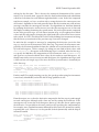
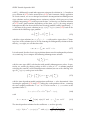
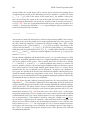
cretization of the governing equations, see [1, 2]. However, for simplicity and succinctness, we will assume the governing equations have already been discretized and
we are looking for methods applying the contact conditions directly on the discretized
form. Many discretizations of the governing equations of elasticity use pure displacement Lagrange FEs, where at some selected sampling points Xi , i = 1 . . . N , three
degree-of-freedoms ui = u(Xi ) ∈ R3 determine the displacement u(X) at Xi . In turn,
the set of sampling points is determined by the finite element mesh and the chosen
degree of the approximation for u(X). Other FEs may add other dofs to determine
the displacement, as for example rotational dofs for shell elements. Here the numerical implementation of contact algorithms will be more complex and not so general, so
that it will be not considered here.
Penalty method
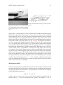
One advantage of the penalty approach to contact mechanics is that it does not necessarily require any modifications of the underlying finite element implementation and
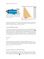
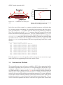
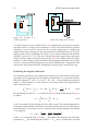
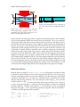
it is solely based on the specification of contact forces in form of tractions. By comparing the known stamp’s position with the actual computed displacements, as soon
the impenetrability condition of both bodies is violated, the penalty method adds stiff
forces T in the direction of the rigid-body normal n, in order to restore the impenetrability condition. Actually this latter condition can only be satisfied approximately
and the degree of approximation is controlled by a penalty parameter. The dilemma is
that the better the impenetrability approximation is, the worse is the ill-conditioness
of the system to be solved and computing solutions will be slower and harder. For a
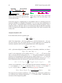
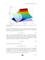
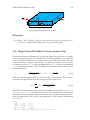
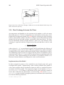
generic boundary point x = X + u with rigid-body projection x0 , let δ be the actual
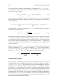
value of penetration defined by δ = (x0 − x) · n. The penalty method defines the tractions as T = h(δ)n with h(δ) a stiff function having the properties h(δ ≤ 0) = 0 and
h(δ ≥ 0) ≥ 0. A good working example is h(δ) = aδb with a ≫ 1 and b = 2.
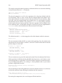
In order not to further slow down the non-linear solution process, we need to correctly
specify the traction’s derivatives ∂u T with respect to the displacements u in order to
assemble a global exact Jacobi matrix and to guarantee a quadratic convergence rate
of the Newton iteration close to the solution. For this task, we need a second order
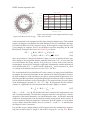
approximation of the surface at x0 given by
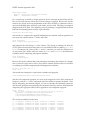
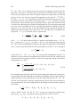
s(p1 , p2 ) = x0 + tα pα + nkα p2α /2 + O(|(p1 , p2 |3 ) ,
with free parameters pα and an implied sum over the indices α. The closest point
projection of any point x close to x0 is approximately given by x̄0 (p1 , p2 ) = s(p1 , p2 )
with pα = (x − x0 ) · tα (1 + δkα )−1 + O(|x − x0 |2 ). By expressing the surface normal as
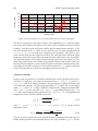
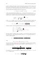
n̄(p1 , p2 ) =
=
∂p1 s × ∂p2 s
(t1 + p1 k1 n) × (t2 + p2 k2 n)
=
|∂p1 s × ∂p2 s|
|∂p1 s × ∂p2 s|
n − pα kα tα
t1 × t2 + p2 k2 t1 × n + p1 k1 n × t2 + p1 p2 k1 k2 n × n
,
= p
|∂p1 s × ∂p2 s|
1 + p2α kα2
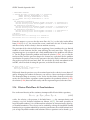
we have ∂pα n̄|pα =0 = −kα tα and by the chain rule ∂x n̄ = (∂pα n̄)(∂x pα ) = −kα /(1 +
δkα )tα ⊗tα . In a similar way, we obtain ∂x x̄0 = (∂pα x̄0 )(∂x pα ) = −kα tα ⊗tα . It follows