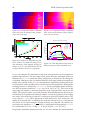
1
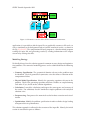
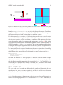
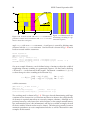
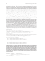
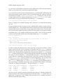
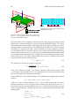
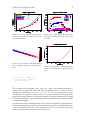
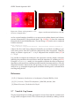
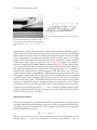
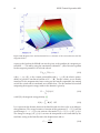
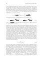
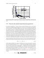
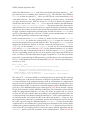
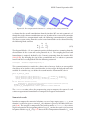
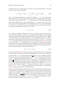
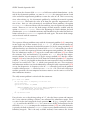
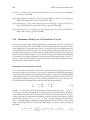
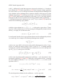
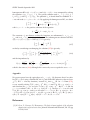
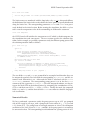
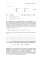
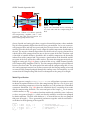
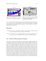
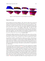
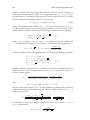
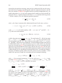
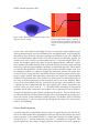
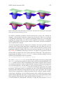
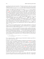
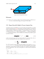
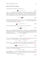
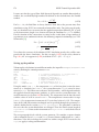
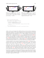
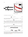
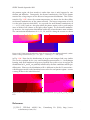
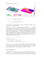
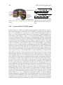
SESES Tutorial September 2012
155
Figure 2.103: Initial and intermediary deformations with final state showing the spring-back
effect. Just half of the structure is shown.
the model is rotational symmetric and the material laws used in this example are
isotropic, a 2D rotational symmetric solution may do the job. However, we present
a 3D problem formulation, since in practice anisotropic plastic laws are needed thus
requiring 3D computations even for an initial symmetry of revolution. In addition
realistic computations will also require contact with frictions, instead of friction-less
ones as done in this example.
An initial rectangular laminate clamped at its border is all what is needed as initial
geometry, if the closest point projection is computed by the user. However, for a visual aid in the graphical representation, it is also useful to define the geometry of the
rigid-body stamps by dummy MEs where no numerical equation is ever solved, see
Fig. (2.103). An additional advantage is that one can right use the geometry of these
dummy MEs to compute the closest point projection numerically. This projection is
computed by the routine RigidIntersection, however, before calling it, one has
to declare the rigid-bodies with the statement
Misc RigidBody(StampDown Down, StampUp Up; Smooth)
The values StampDown-StampUp are the block ME numbers for the two stamps and
the Down-Up specifiers determine the contact surface of the hexahedral ME block. The
Smooth option activates cubic interpolation so that normal, tangents and curvatures
are continuous functions. In this example both the analytical and numerical approach
are used and compared. For the former, a series of input routines ParabolaProj,
Profile, StampCoord, StampProj is defined evaluating the projection as described
previously. Typo errors in these user routines are not so easily discovered and within
comments some additional testing code that has been used is provided. The selection
of one of the two approaches is simply determined by the setting of a global variable.
At the input’s beginning, we have defined routines to be used by the penalty and algebraic contact approach. Since they are pretty generic, they can be placed once inside
some input files to be included. For the penalty method, the routine PenaltyContact
is used to define the Neumann BCs and takes as input the data structure CONTACT