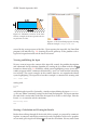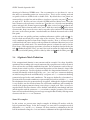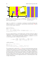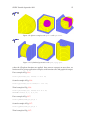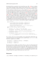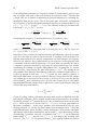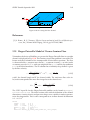
1
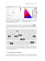
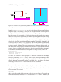
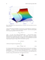
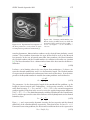
SESES Tutorial September 2012
19
drawing of a Bézier or NURBS curve. Due to symmetries, we just draw 90◦ arcs so
that only two controlling points are necessary here. These are the starting and end
arc points which are defined with a double click. By default these two points are
connected by a straight line and to define a circular arc, open the arc panel and set
an angle of 90◦ . Be sure you have selected a NURBS and not a Bézier curve, since this
latter cannot exactly represents a circular arc. If not the case, select the two controlling
points and apply the rational segment option . After a curve has been defined, one
has to attach macro element nodes to the curve. With the attach task , pick a macro
element node, drag it over the curve until a snap takes place and move the node along
the curve at the correct position. Attached nodes are marked afterwards with a thick
blue point.
At the end one can quickly perform a uniform refinement with the split task . Select the whole mesh and pick a single edge of the selection. These simple shapes are
easily combined together to form more complex meshes. Here, it is better to work
with unrefined and coarse meshes and to perform the uniform refinement just as last
operation on the whole mesh. The construction process is almost the same as for the
basic shapes. With copy&paste operations, selections are duplicated and with the join
task
combined together. Here, you may first need to mirror the duplication along
the x- or y-axis before joining, which is done by affine task and the affine panel .
1.6 Algebraic Mesh Definition
If the computational domain is non-constant and for example if its shape should be
optimized, then working with a mesh constructed by a preprocessor is not well suited,
since such meshes are hardly modified afterwards. For an automatic search of the optimum, better suited is to have a functional dependency of the domain’s shape from
some free parameters. For this algebraic method, the computational domain is constructed functionally with the help of the QMEI, QMEJ and QMEK statements defining
an initial rectangular mesh and followed by a sequence of Coord statements defining
geometrical maps for the node coordinates. The maps are defined by a functional expression of the latest node coordinates represented by the built-in variables x,y,z and
the subdomain where the geometrical map is applied. Although this algebraic method
is very flexible, one first needs to know the actual node coordinates and secondly the
search of the proper geometrical map is not always a simple task. Here, several rectangular blocks of macro elements can be defined, individually transformed and later
joined together with the statement JoinME to form a complex geometry. This is often
more convenient than defining just one huge rectangular block and by deleting macro
elements with the DeleteME statement.
Some 2D examples
In this section, we present some simple examples of defining 2D meshes with the
help of geometrical maps. In the first example, we start with a rectangular mesh of
dimension lx∗ly and of nx∗ny elements. We then translate a subdomain in the left
half of our domain along the x-axis and rotate a subdomain of the right half about the