1
A.R.M. Loxahatchee National Wildlife Refuge
Simple Refuge Screening Model (v. 4.0)
User’s Manual
Ehab A. Meselhe
Michael G. Waldon
William B. Roth
Prepared for the U.S. Fish and Wildlife Service under a
cooperative-agreement with the University of Louisiana-Lafayette
Report #LOXA009-002
April 2009
SRSM Version 4.00 User’s Manual
A.R.M. Loxahatchee National Wildlife Refuge Simple Refuge Screening Model
Version 4.00 Report #LOXA009-002
User’s Manual
Ehab Meselhe1, Mike Waldon2, William Roth1
1. Introduction
As restoration of the Arthur R. Marshall Loxahatchee National Wildlife Refuge (Refuge)
continues, there is a need for a simple, quantitative methodology for predicting impacts
of proposed management changes on Refuge stage. The Simple Refuge Screening Model
(SRSM) simulates the water budget, regulation schedule implementation, and constituent
dynamics for chloride (Cl), sulfate (SO4), and total phosphorus (TP). This document
presents the model in a format that provides users with an understanding of both the
theory and implementation of the SRSM. The objective is to give users the ability to
accurately simulate various water need scenarios for the Refuge in order to gain a better
understanding of this wetlands system and its dynamics. This manual assumes that the
reader is generally familiar with the location Refuge hydrologic features, and with water
quality issues relevant to the Refuge. For more information, users are directed to the
Refuge Comprehensive Conservation Plan (USFWS 2000).
This manual describes version 4.00 of the SRSM. SRSM version 1 was implemented by
Jeanne Arceneaux and others (Arceneaux, 2007; Arceneaux et al., 2007; Meselhe et al.,
2007) as a daily water budget using Microsoft Excel; the results from this model were
then used to drive the constituent model. The constituents were modeled by WASP, a
program developed by the United States Environmental Protection Agency. Although
there were advantages in using a commonly available spreadsheet program paired with a
proven, robust constituent modeling tool, there were also some clear disadvantages. The
version 1 implementation was complex and did not easily lend itself to modification. The
workbook file was large, and its size grew as more days were simulated. Additionally,
the limitation of using a one-day step size required ad-hoc procedures to avoid instability
of the solution. Finally, the constituent models in WASP are limited to those provided in
the closed-source executable from the USEPA. These factors and a desire to have a
single, consistent model platform led to porting the stage and water quality models to the
STELLA (http://www.iseesystems.com/index.aspx) simulation platform (version 2).
Version 3 of the models ported the earlier version programs to the Berkeley Madonna
(http://www.berkeleymadonna.com/index.html) simulation platform. In versions 2 and 3,
stage and constituent models were separate. In version 4, models for stage and
constituent concentration were combined into a single Madonna program. Use of the
Berkeley Madonna commercial numerical differential equation solver package allows
greater clarity in coding, supports shorter time steps obviating the need for the ad-hoc
procedures of version 1, and provides a well documented user interface.
1
2
Center for Louisiana Water Studies, University of Louisiana at Lafayette
A.R.M Loxahatchee National Wildlife Refuge, U.S. Fish and Wildlife Service
2
SRSM Version 4.00 User’s Manual
1.1. General Description of Model Structure
To calculate water volume the SRSM version 4.00 divides the Refuge into two
compartments (also termed boxes or cells), Canal and Marsh, with assumed constant
areas of 4.03 million m2 and 560.02 million m2, respectively. The rate of change of
compartment volumes are calculated using the following differential equation which
is based on the water budget for each compartment:
dVi
Qnet Ai P Gi ETi
dt
where:
i = denotes compartment (marsh or canal),
Vi = the compartmental volume (m3),
t = time (days),
Qnet = total flow into a compartment (m3/day),
Ai = compartment surface area (m2),
P = precipitation (m/day),
Gi = loss due to groundwater seepage (m/day), and
ETi = loss due to evapotranspiration (m/day).
SRSM version 4.00 simulates the mass and concentration of chloride (Cl), total
phosphorus (TP), and sulfate (SO4). Note that TP mass is measured as phosphorus,
not phosphate, and SO4 mass is measured as sulfate, not sulfur. The compartmental
design for these calculations differs from the water balance simulation. Here, a
concentric arrangement of 4 compartments is used to represent the Refuge.
Compartments 1-3 disaggregate the water-budget marsh compartment; compartment
4 represents the canal. Exchange flow is calculated in the marsh based on
compartment surface area ratios. Calculation of flow between marsh cells 1-2 and 23 is made using a flat-pool assumption, and is analogous to a tidal prism flow
calculation.
All constituents are simulated based on a mass balance equation. The loading terms
of the mass budget (qnet, gload, and aload) are similar in all three constituents.
However, the reactive load term (rload) is uniquely structured for each constituent.
Chloride is modeled as a conservative constituent with zero reactive load. Its mass is
lost or gained solely through the transport of water into or out of the system;
therefore, the rload term in the following equation should be ignored when chloride is
considered. Total Phosphorus (TP) dynamics are approximated with equations
adapted from those presented in the Dynamic Model for Stormwater Treatment Areas
(DMSTA) developed by Walker and Kadlec3. Finally, sulfate (SO4) dynamics are
simulated using a Monod relationship. Thus, a general equation for the rate of change
of constituent mass in a compartment is given by:
3
http://wwwalker.net/dmsta/index.htm
3
SRSM Version 4.00 User’s Manual
dM i , j ,k
dt
qneti , j ,k gloadi , j ,k aloadi , j ,k rloadi , j , k
where:
i = constituent,
j = compartment number (1-4),
k = DMSTA calibration set (Phosphorus only),
M = mass (g),
t = time (days),
qnet = net mass flow in surface water (g/day),
gload = loss to groundwater seepage and evapotranspiration (g/day),
aload = gain from wet and dry deposition (g/day), and
rload = loss to storage uptake/release (TP) or reaction (SO4) (g/day).
Detailed descriptions of the above equations can be found in the companion model
manuscript (Waldon et al., 2009).
1.2. Model Platform – Berkeley Madonna
The SRSM version 4.00 is implemented using the differential equations solver
Berkeley Madonna version 8.3.9 (Madonna), which is a proprietary software
developed by Robert I. Macey and George F. Oster. This program is the backdrop for
the code of the SRSM, and while Madonna has some built-in functions, all SRSM
components and processes are user-defined in the Equations window; the optional
Madonna Flowchart window was not used in SRSM development (in terms used in
Madonna documentation, SRSM is a “plain-text” rather than a “visual” model).
Figure 1 shows the general format of the Madonna desktop. These windows may be
resized or closed by the user. Each of these windows is discussed later in this
document.
Madonna also has the capability to perform optimizations, curve-fitting, and
sensitivity analyses. For a comprehensive description of all pre-programmed
functions, users of the SRSM are encouraged to download the Madonna user’s guide
from www.berkeleymadonna.com. Additionally, users may download a demo
version of this software from the Berkeley Madonna web site and run this version of
the SRSM version 4.004. However, while the demo version of the Madonna program
allows users to modify and run models, the demo version does not allow the user to
save model files or output of any kind.
4
Available for download at: http://loxmodel.mwaldon.com/
4
SRSM Version 4.00 User’s Manual
Figure 1 – Madonna model desktop
1.3. User’s Manual Objectives
This manual presents the pertinent information required for users to understand the
components of SRSM (i.e., imported data, SRSM equation format, and postprocessing methods). Ultimately, users should use this document as a companion for
the model to assure accurate execution and interpretation.
1.4. Caveats
1.4.1. If unfamiliar with Berkeley Madonna, SRSM users are strongly urged to
consult the user’s guide before attempting to run or manipulate any of the
model components.
1.4.2. All parameter values represent those used to accurately validate and
calibrate this model; discretion should be used when altering these values.
1.4.3. This model is set up to simulate a 13-year (1995-2007) period. All time
series data needed to successfully run the model are stored within the
model file. This manual provides the user with the background and
understanding needed to revise this model simulation for other userselected time periods or scenarios. Should the user want to simulate
another time period or alternative conditions, the proper data must be
obtained, properly formatted, and imported into the model.
5
SRSM Version 4.00 User’s Manual
1.4.4. Because of the level of spatial aggregation in the SRSM, the SRSM is not
appropriate for applications that involve site-specific events. All results
should be considered as spatial average values for the area of study.
1.4.5. This document offers a brief summary of model theory and equations.
Users should consult the referenced documentation, the model code, and
the companion manuscript for more in-depth descriptions of equations and
calibration parameter values.
2. Data Preparation
This section describes how to import the necessary time series text files. The 7 separate
data input files are outlined in Table 1.
Filename
Data Vectors
Summary
CL.txt
14
Chloride concentration values (mg/L)
INFLOW.txt
20
Historic inflow values (m3/d)
OUTFLOW.txt
20
Historic outflow values (m3/d)
PET.txt
3
Precipitation and Evapotranspiration (m/d)
Regulation.txt
5
Water supply release from S-39 and hurricane
releases from S-10 structures (m3/d)
SO4.txt
14
Sulfate concentration values (mg/L)
TP.txt
14
TP concentration values (mg/L)
(alphabetical)
Table 1 – SRSM input files
Users may create data files for import in any spreadsheet editing program. Madonna
imports data files in either tab-delimited text format or comma-separated values (CSV)
format. The preloaded input files in the SRSM are primarily derived from data
downloaded from the South Florida Water Management District’s database
(DBHYDRO5). Although these data are readily available, and methods of preparation
documented (Arceneaux, 2007; Meselhe et al., 2005), it is strongly suggested that the
user first run model simulations with the preloaded datasets.
5
http://www.sfwmd.gov/portal/page?_pageid=2894,19708232&_dad=portal&_schema=PORTAL
6
SRSM Version 4.00 User’s Manual
2.1. Spreadsheet Formatting
The Berkeley Madonna software imports time series data from a 2-dimensional array
dataset. The first column of the array is the time value in days of the simulation
beginning with zero and increasing monotonically to the final simulation day (in this
case, 0 to 4747). Madonna applies linear interpolation between data values. In order
to avoid interpolation in the time series data, the user is encouraged to format the time
series such that there are two values (the same value) for each time period (e.g., t1.000
= 5.656 and t1.999 = 5.656); thus, the imported data become similar to a step function.
To minimize the effort, a data organization subroutine may be written into a Visual
Basic for Applications (VBA) module in Microsoft Excel. Additionally, the user
must note that text and other non-numerical symbols will not be imported into
Madonna; in fact, the importing process will cease if Madonna encounters such a
symbol. As a reference, an abbreviated example spreadsheet, along with its VBA
data organization subroutine, is provided in the Appendix of this document.
2.2. Importing Data
Once a dataset has been created, it may be imported into Madonna by choosing
Import Dataset from the File menu. The user is then prompted to specify the dataset
type and filename; in this case all datasets are entered as 2D and given a specified
filename per Table 1 (the file extension should not be included). Madonna syntax
requires that the name of the input file be preceded by a pound sign (#). Typically,
for 2-dimensional datasets a timing variable must be given; this variable tells
Madonna at which times to read imported data. A simple solution is to use the build
in function named TIME. In Madonna the syntax TIME represents a linear function
that counts from the specified start time (STARTTIME) value to the specified stop
time (STOPTIME) value based upon the time step (DT). The following equations
set variables for precipitation (P) and evapotranspiration (ET) to the appropriate
imported time series data values:
P = #PET(day,1); (m/day)
ET = #PET(day,2); (m/day)
where #PET indicates the file of imported data being used, day is the integer day of
the simulation, and the numerical value indicates a column in the imported dataset.
Once data are successfully imported, the file name will appear in the Datasets
window on the Madonna desktop. Additionally, it is important to note that imported
data are saved directly in the Madonna model file (*.mmd). There is no dynamic link
between these data and the parent spreadsheet; therefore, any changes to the time
series data must be made in the parent *.csv or *.txt file and then re-imported into the
Madonna model.
3. Comments, Constant Values, Arrays, & Equations
7
SRSM Version 4.00 User’s Manual
Comments within the equation window provide model self-documentation, and are an
important part of the SRSM documentation. There are two alternative syntaxes for
comments in Madonna. Any text between left and right curly brackets, { }, is treated as a
comment and not processed. This form of comment can span multiple lines of text. On a
single line, all text following a semi-colon is also treated as a comment.
Additionally, in imported text data files, all characters on a line following the first nonnumeric character are ignored. This allows comments identifying source or column
names to be included within these files.
Equation syntax in Berkeley Madonna is similar to that in other programming languages
such as Basic or FORTRAN. The value calculated on the right-hand-side of an equals
sign is assigned to the variable on the left-hand-side. Unlike common programming
languages, but similar to spreadsheets, Berkeley Madonna is non-procedural; meaning the
ordering of the equations is not significant. Berkeley Madonna effectively sorts the
equations in order to calculate the value of variables before they are used in subsequent
calculations; the program recognizes circular references if such a sorting can not be
accomplished (Macey et al., 2000).
Many of the SRSM equations have been consolidated by using arrays. Such equations
are set up by using the square brackets ([]) for the values to be arrayed. There are 3 sets
of arrayed variables: constituents, compartment, and DMSTA calibration sets. For all
equations displayed in sections labeled 3.4.(3-8) the user can see examples of arrayed
initial conditions and differential equations. Labels for each of the arrayed variables are
given below.
Arrays are used extensively in SRSM to express equations that are repeated for a range of
cells or constituents. Many of the array index values have been programmed as constants
to enhance clarity of the code. For example, the equation “tp=3” defines a constant
named tp that can be used as an array index (subscript) in place of simply the more
obscure number 3. Madonna does identify constants during compilation, and there is
apparently no runtime cost associated with this programming style.
;DEFINE ARRAYS
;REFUGE GEOMETRY
ncell=4; total number of cells, canal is cell ncell
nm=ncell-1; number of marsh cells
canal=ncell; cell number for canal (there is only 1 canal cell in version 4.00)
;CONSTITUENTS
nconstit= 3
cl= 1; chloride; conservative
so4=2; sulfate; monod relationship;
tp= 3; tp modeled with DMSTA equations
;DMSTA CALIBRATION SETS
emerg = 1; Emergent marsh
pew = 2; Pre-existing wetland
8
SRSM Version 4.00 User’s Manual
Madonna has a unique notation for array operations (Macey et al., 2000). Equations
imply looping through a range of subscripts through ranges specified on the left-handside of the equation (see for examples sections 3.4.5 and 3.4.6 below). The variables i, j,
and k are reserved in Madonna to refer on the right-hand-side of the equation to the first,
second, and third array index, respectively, of the variable on the left. This notation
replaces loops that are more commonly used in other programming languages.
3.1. Runtime Options
Madonna offers several numerical methods to solve ODEs. The SRSM may be
executed accurately and expeditiously using the RK4 (fourth order Runge-Kutta)
method.
The current SRSM is set up to simulate the 13 year period from 1995 to 2007. The
user may specify the simulation period with the STARTTIME and STOPTIME
functions. Model coding for the runtime parameters is given below.
3.1.1. Code
METHOD RK4
STARTTIME = 0 {JAN95}; 3287 {JAN04}; 1826 {JAN00};
STOPTIME= 4747 {DEC07}; 3652 {DEC04}; 4382 {DEC06};
DT = 0.005
DTOUT = 1
By default, Madonna saves model output every calculation time step, which can
become costly as model size and complexity increases. The built-in variable
DTOUT defines the time period that elapses between data storage for a
simulation run. Setting DTOUT can reduce memory requirements. Here, SRSM
output is stored every one time unit (i.e., one day). If the user desires to store all
output data, then DTOUT should be set equal to zero or, alternatively, the
DTOUT statement can be removed.
3.2. Parameters
These values fall into two categories for the SRSM code – simulation option
parameters, and model parameters. The simulation option parameters are given at the
beginning of the model code (found in the Equations window). These allow some
flexibility with model calculations, input data, and initial conditions. The user can
choose outflow type, scale flow and constituent load, choose time series or constant
values for boundary concentration, and choose different initial condition sets. The
remaining parameters are calibrated and calculated values needed for an accurate base
simulation of the SRSM.
9
SRSM Version 4.00 User’s Manual
All model parameters (constant values) that are not arrayed can also be viewed in the
Parameters window, which allows the user to change values and reset them without
directly changing the code. Parameters with values modified from those set in the
Equations window are flagged by an asterisk in the Parameters window. Users are
cautioned that if parameter values are changed using the Parameter window, the
altered values may persist in future model runs until they are reset. Additionally, the
Overlay Plots (Figure 3) button can be used to display multiple model runs on the
same graph; this feature is very helpful when visually assessing parameter alterations.
Lists of all parameters are given in the appendix of this document.
3.3. Processes
Model processes are those equations that contribute to state variable calculation (e.g.
groundwater seepage, corrected evapotranspiration, and reaction losses). Such
equations represent values that can change with each time step. The user should
consult the referenced material for more in depth discussions and explanations of
model processes.
3.4. State Variables
Berkely Madonna has several ways to code state variables. The SRSM uses the
d/dt() option to define differential equations. All SRSM differential equations are
given below. It is necessary to specify an initial value for all state variables using the
INIT initializer syntax.
This version of the SRSM directly calculates the change in volume of the Canal and
Marsh compartments as per the 2-compartment structure described by Arceneaux et
al. (2007). The stage is then calculated from the volume. It must be noted that the
area of the compartments is constant (i.e., it does not change with stage). The
calculated value for the exchange flow (canal to marsh flow) is used to drive the
volume differential equations for the 4-compartment constituent model.
3.4.1. Initial Volume Values: 2-compartment Model
INIT vol_canal = (Ecinit - Eoc) * Canal_Area; Initial Canal Volume (m3)
INIT vol_marsh = (Eminit - Eo) * Marsh_Area; Initial Marsh Volume (m3)
3.4.2. Volume Differential Equations: 2-compartment Model
d/dt(vol_canal) = NetInFlow - Exchange_Flow +((P- Gc - ETc)*Canal_Area)
d/dt(vol_marsh) = Exchange_Flow +((P - Gm - ETm)*Marsh_Area)
3.4.3. Initial Volume Values: 4-compartment Model
INIT vol[1..nm] = (Eminit - Eo) * area[i]
INIT vol[canal] = (Ecinit - Eoc) * area[canal]
3.4.4. Volume Differential Equations: 4-compartment Model
10
SRSM Version 4.00 User’s Manual
d/dt(vol[canal])= Qin - Qout - Exchange_Flow + ((P-ETc-Gc)*area[canal])
d/dt(vol[1..nm])= ((P-ETm-Gm)*area[i]) + (Exchange_Flow*qmcfactor[i])
In addition to volume state variables the SRSM calculates storage and constituent
mass similarly.
3.4.5. Initial Mass Values: Chloride Only
INIT mass[cl,1,emerg..pew]= D_M0*area[1]* INIT_Conc[i,j,k]
INIT mass[cl,2,emerg..pew]= D_M0*area[2]* INIT_Conc[i,j,k]
INIT mass[cl,3,emerg..pew]= D_M0*area[3]* INIT_Conc[i,j,k]
INIT mass[cl,canal,emerg..pew]= D_C0*area[canal]* INIT_Conc[i,j,k]
3.4.6. Mass Differential Equations
{COMPARTMENT 1} d/dt(mass[1..nconstit, 1,emerg..pew]) = qload[i, 1,k] - qload[i, 2,k]
+ aload[i, 1] - gload[i, 1,k] + rload[i, 1,k]
{COMPARTMENT 2} d/dt(mass[1..nconstit, 2,emerg..pew]) = qload[i, 2,k] - qload[i, 3,k]
+ aload[i, 2] - gload[i, 2,k] + rload[i, 2,k]
{COMPARTMENT 3} d/dt(mass[1..nconstit, 3,emerg..pew]) = qload[i, 3,k] + aload[i, 3] gload[i, 3,k] + rload[i, 3,k]
{COMPARTMENT 4} d/dt(mass[1..nconstit, canal,emerg..pew]) = sload[i,j,k] - qload[i,
1,k] + aload[i, canal] - gload[i, canal,k] + rload[i, canal,k]
3.4.7. Initial Storage Values
INIT dmsta_store[tp, 1..nm, emerg..pew]= init_storage[i,j,k] ; g/m2
3.4.8. Storage Differential Equations
d/dt(dmsta_store[tp, 1..nm, emerg..pew])= upPrM2[i, j,k] - ((Release[i, j,k] + Burial[i,
j,k])/area[j])
3.5. Volume-Stage Relationship
SRSM version 4.00 is structured to incorporate a storage-stage relationship for both
the marsh and canal compartments. To maintain consistency with the earlier model
version, a constant surface area is currently assumed for each compartment resulting
in a linear relationship between storage volume and stage. Canal (Ec) and marsh
(Em) stage values in meters are calculated using the GRAPH capability of Madonna.
Future versions of the SRSM could include a more detailed volume-stage
relationship. However, performance of the model is good without the addition of this
complexity.
;Stage (m) NGVD 29 is currently calculated using constant area
;
( Vc(m3), Ec(m)) Area Canal = 4033485.467 (m2)
Ec = GRAPH (Vc) (-13068492.91,0) (0, 3.24 {Canal bottom elevation}) (27266361.76, 10)
11
SRSM Version 4.00 User’s Manual
;
( Vm(m3), Em(m)) Area Marsh = 560021212.8 (m2)
Em = GRAPH (Vm) (-2587298003, 0) (0, 4.62 {Marsh bottom elevation}) (3012914125, 10)
4. Regulation Schedule
This document assumes that SRSM users are familiar with this WCA-1 Regulation
Schedule (USACE 1994), as its specifics are not included here. A description of the
Regulation Schedule is available in the Arthur R. Marshall Loxahatchee National
Wildlife Refuge Comprehensive Conservation Plan (USFWS 2000). The following subsections present the Regulation Schedule model code which appears in the Madonna
Equations window.
The variables A1FloorFeet and BFloorFeet are the stage in feet (NGVD) of the bottom of
the A1 and B Regulation Schedule zones, respectively. For consistency with the SRSM,
these variables are converted to meters.
A1FloorFeet = GRAPH(DayofYear) (0,17.2) (132, 15.75) (188, 15.75) (267, 17.5) (334, 17.5)
(366, 17.2); Floor of A1 Zone (ft)
BFloorFeet = 14; Floor of B Zone (ft)
A1Floor = A1FloorFeet*0.3048; A1 Floor (m)
BFloor = BFloorFeet*0.3048; B Floor (m)
4.1. SRSM Regulatory Release
A regulatory release is a discharge of water out of the Refuge that occurs as a result
of the Refuge stage in relation to the Regulation Schedule. Magnitude of outflow
during a regulatory release is not specified within the Regulation Schedule. It is
therefore necessary to make assumptions related to water management in order to
model regulatory releases. The prior version of the SRSM modeled regulatory
releases based on historic discharges.
4.2. Regulatory Release Calculations
This section describes calculations used in the Regulation Schedule. Outflow is
calculated when the CalcQRo value (in the simulation option parameters section) is
set to a value of 1; conversely, a value of 0 uses historical outflow in the model
simulation. The calculated outflow only represents regulatory releases from certain
structures (S10ACDE and S39); therefore, historic outflows from other structures in
the Refuge must be imported to supplement the calculated outflow.
Qout = IF (CalcQRo = 0) THEN (QoutHistoric) ELSE (QoutCalc + QWaterSupply +
Qout_HistStruct + Qout_hurricane)
Qout_HistStruct = G94A_out + G94B_out + G94C_out + G300_out + S5AS_out + G301_out
+ G338_out; Structures in the north and east involved with water supply
12
SRSM Version 4.00 User’s Manual
; Regulatory release (thousand m3/d) as a function of difference between stage and A1 zone
floor (ft).
; This is based on historic S10 flow 1/1/1995 - 8/31/2007 initially copied from file CA1elevations.xls
QoutCalcS10 = GRAPH((Ec-A1Floor)/0.3048) (-1.3,0) (-1.2,32) (-1.1,113) (-1,64) (-0.9,94) (0.8,148) (-0.7,311) (-0.6,238) (-0.5,175) (-0.4,328) (-0.3,288) (-0.2,450) (-0.1,765) (0,957)
(0.1,1323) (0.2,2274) (0.3,3188) (0.4,2832) (0.5,4469) (0.6,5901) (0.7,7406) (0.8,6602)
(0.9,6356) (1,8116)
;Reduction factor & Scale up S10 regulatory flows by ratio of total regulatory release/S10,
convert thousand m3/d to m3/d
QoutCalc =RSQfact*(196.7/144.8)*1000*QoutCalcS10
The ratio 196.7/144.8 is the historic average annual total Refuge regulatory release
volume divided by the average annual S-10 volume.
5. Model Execution & Post-processing
Berkeley Madonna’s user interface for model execution and post-processing is very
simple; in fact, they can both be operated from a single location. All operations needed
for a general simulation run can be performed in the Graph window. The provided
image designates the pertinent buttons with which the user should be familiar; however,
for explicit explanations on each button, the Berkeley Madonna user’s guide (Macey et
al., 2000) should be consulted. The model may be executed from the Graph window by
pressing the Run button; otherwise, the user may select Run from the Compute menu.
Figure 2 – Graphical Output
13
SRSM Version 4.00 User’s Manual
Figure 3 – Graph Toolbar
After pressing the Run button, Madonna will automatically output several variables from
the model in the Graph window. To specify which variables to output, the user can
double-click in the window and choose them from a list or select Choose Variables from
the Graph menu. Once the desired variables are chosen and a model run is complete, the
user may print the graph directly from Madonna or export the data as *.csv or *.txt. To
export data the table must be displayed in the Graph window by clicking the Data Table
button (see Figure 3). Then the user can select Export Table from the File menu, or use
the Copy Table selection under the edit drop down menu.
14
SRSM Version 4.00 User’s Manual
For further information, users may contact the authors by email at:
Dr. Ehab Meselhe ([email protected]),
Dr. Mike Waldon ([email protected]), or
William Roth ([email protected])
Citations
Arceneaux, J. (2007). “The Arthur R. Marshall Loxahatchee National Wildlife
Refuge Water Budget and Water Quality Models,” MS. Thesis, University of
Louisiana, Lafayette, LA.
Arceneaux, J., Meselhe, E. A., Griborio, A., and Waldon, M. G. (2007). “The Arthur
R. Marshall Loxahatchee National Wildlife Refuge Water Budget and Water
Quality Models.” Report No. LOXA-07-004, currently available at <
http://loxmodel.mwaldon.com >, University of Louisiana at Lafayette in
cooperation with the U.S. Fish and Wildlife Service, Lafayette, Louisiana.
Macey, R., Oster, G., and Zahnley, T. (2000). “Berkeley Madonna User’s Guide
Version 8.0.” University of California, Department of Molecular and Cellular
Biology, Berkeley, CA.
Meselhe, E., Arceneaux, J., and Waldon, M. G. (2007). “Mass Balance Model
Version 1.01.” LOXA-07-002, currently available at <
http://loxmodel.mwaldon.com >, University of Louisiana - Lafayette in
cooperation with the U.S. Fish and Wildlife Service, Lafayette, LA.
Meselhe, E. A., Griborio, A. G., Gautam, S , Arceneaux, J.C., Chunfang, C.X., 2005.
“Hydrodynamic And Water Quality Modeling For The A.R.M. Loxahatchee
National Wildlife Refuge, Phase 1: Preparation Of Data, Task 1: Data
Acquisition and Processing.” Report #LOXA05-014, University of Louisiana
at Lafayette, prepared for the Arthur R. Marshall Loxahatchee National
Wildlife Refuge, USFWS, Lafayette, LA. Available online:
http://sofia.usgs.gov/lox_monitor_model/advisorypanel/data_acq_report.html.
USACE. (1994). "Environmental Assessment: Modification of the Regulation
Schedule Water Conservation Area No. 1." available at <
http://mwaldon.com/Loxahatchee/GrayLiterature/USACE-1995-LoxRegulation-Schedule.pdf >, US Army Corps of Engineers, Jacksonville, FL.
USFWS. (2000). "Arthur R. Marshall Loxahatchee National Wildlife Refuge
Comprehensive Conservation Plan." available at < http://loxahatchee.fws.gov
>, U.S. Fish and Wildlife Service, Boynton Beach, Florida.
Waldon, M. G., Meselhe, E. A., Roth, W. B., Wang, H., Chen, C. (in prep). “A.R.M.
Loxahatchee National Wildlife Refuge Water Quality Modeling – Rates,
Constants, and Kinetic Formulations.” Report No. LOXA009-003, University
of Louisiana at Lafayette in cooperation with the U.S. Fish and Wildlife
Service, Lafayette, Louisiana.
15
SRSM Version 4.00 User’s Manual
Appendix
1. Example Spreadsheet Format
Figure 4 – Sample Excel Spreadsheet
2. Data Formatting with VBA
Sub LoopRange1()
'have x & z start at row 2
'have y start at row 3
x = 2
z = 2
y = 3
‘loop until a blank row is found
‘for the purposes of this we need a column of 7306 (3653*2) values
‘in order to separate the input data appropriately.
‘note that this is set up for data to be read only in column 2 (date column)
‘and for the sorted data to be output in columns B, C, D, E, F and G.
Do While Cells(x, 1).Value <> ""
'This will put the values of the
'9th column (I) in the 2nd
'column (B) such that data
'abcd... become aabbccdd...
Cells(x, 2).Value = Cells(z, 9).Value
Cells(y, 2).Value = Cells(z, 9)
Cells(x, 3).Value = Cells(z, 10).Value
Cells(y, 3).Value = Cells(z, 10)
Cells(x, 4).Value = Cells(z, 11).Value
Cells(y, 4).Value = Cells(z, 11)
Cells(x, 5).Value = Cells(z, 12).Value
Cells(y, 5).Value = Cells(z, 12)
16
SRSM Version 4.00 User’s Manual
Cells(x, 6).Value = Cells(z, 13).Value
Cells(y, 6).Value = Cells(z, 13)
Cells(x, 7).Value = Cells(z, 14).Value
Cells(y, 7).Value = Cells(z, 14)
‘increse the value of x by 2 in order to create the spacing and increase the
‘value of z by 1 to read the data in the correct order (ie row by row).
‘Y increases by 2 to insert data in rows "skipped" by x+2 term.
x = x + 2
z = z + 1
y = y + 2
Loop
End Sub
3. Imported Datasets
Provided below is a list of all imported datasets and their respective variable
names used in the SRSM.
Variable Name
File
Column
Description
P
PET
1
Area average precipitation (m/day)
Observed evapotranspiration (m/day)
ET
PET
2
S39_out
OUTFLOW
1
Observed structure outflow (m3/day)
G94A_out
OUTFLOW
2
Observed structure outflow (m3/day)
G94B_out
OUTFLOW
3
Observed structure outflow (m3/day)
G94C_out
OUTFLOW
4
Observed structure outflow (m3/day)
G300_out
OUTFLOW
8
Observed structure outflow (m3/day)
S5AS_out
OUTFLOW
9
Observed structure outflow (m3/day)
G301_out
OUTFLOW
11
Observed structure outflow (m3/day)
G338_out
OUTFLOW
15
Observed structure outflow (m3/day)
S10E_out
OUTFLOW
16
Observed structure outflow (m3/day)
S10D_out
OUTFLOW
17
Observed structure outflow (m3/day)
S10C_out
OUTFLOW
18
Observed structure outflow (m3/day)
S10A_out
OUTFLOW
19
Observed structure outflow (m3/day)
G94A_in
INFLOW
2
Observed structure inflow (m3/day)
G94C_in
INFLOW
4
Observed structure inflow (m3/day)
G94D_in
INFLOW
5
Observed structure inflow (m3/day)
ACME1_in
INFLOW
6
Observed structure inflow (m3/day)
S362_in
INFLOW
7
Observed structure inflow (m3/day)
G300_in
INFLOW
8
Observed structure inflow (m3/day)
S5AS_in
INFLOW
9
Observed structure inflow (m3/day)
S5A_in
INFLOW
10
Observed structure inflow (m3/day)
G301_in
INFLOW
11
Observed structure inflow (m3/day)
G310_in
INFLOW
12
Observed structure inflow (m3/day)
G251_in
INFLOW
13
Observed structure inflow (m3/day)
S6_in
INFLOW
14
Observed structure inflow (m3/day)
G338_in
INFLOW
15
Observed structure inflow (m3/day)
S10A_hurricane
Regulation
1
Supplementary emergency water release (m3/day)
S10C_hurricane
Regulation
2
Supplementary emergency water release (m3/day)
17
SRSM Version 4.00 User’s Manual
S10D_hurricane
Regulation
3
S39_WS
Regulation
4
Supplementary emergency water release (m3/day)
Supplementary water supply release (m3/day)
G94A_TP
TP
1
Observed total phosphorus concentration (mg/L)
G94C_TP
TP
2
Observed total phosphorus concentration (mg/L)
G94D_TP
TP
3
Observed total phosphorus concentration (mg/L)
ACME1_TP
TP
4
Observed total phosphorus concentration (mg/L)
S362_TP
TP
5
Observed total phosphorus concentration (mg/L)
G300_TP
TP
6
Observed total phosphorus concentration (mg/L)
S5AS_TP
TP
7
Observed total phosphorus concentration (mg/L)
S5A_TP
TP
8
Observed total phosphorus concentration (mg/L)
G301_TP
TP
9
Observed total phosphorus concentration (mg/L)
G310_TP
TP
10
Observed total phosphorus concentration (mg/L)
G251_TP
TP
11
Observed total phosphorus concentration (mg/L)
S6_TP
TP
12
Observed total phosphorus concentration (mg/L)
G338_TP
TP
13
Observed total phosphorus concentration (mg/L)
G94A_Cl
CL
1
Observed chloride concentration (mg/L)
G94C_Cl
CL
2
Observed chloride concentration (mg/L)
G94D_Cl
CL
3
Observed chloride concentration (mg/L)
ACME1_Cl
CL
4
Observed chloride concentration (mg/L)
S362_Cl
CL
5
Observed chloride concentration (mg/L)
G300_Cl
CL
6
Observed chloride concentration (mg/L)
S5AS_Cl
CL
7
Observed chloride concentration (mg/L)
S5A_Cl
CL
8
Observed chloride concentration (mg/L)
G301_Cl
CL
9
Observed chloride concentration (mg/L)
G310_Cl
CL
10
Observed chloride concentration (mg/L)
G251_Cl
CL
11
Observed chloride concentration (mg/L)
S6_Cl
CL
12
Observed chloride concentration (mg/L)
G338_Cl
CL
13
Observed chloride concentration (mg/L)
G94A_SO4
SO4
1
Observed sulfate concentration (mg/L)
G94C_SO4
SO4
2
Observed sulfate concentration (mg/L)
G94D_SO4
SO4
3
Observed sulfate concentration (mg/L)
ACME1_SO4
SO4
4
Observed sulfate concentration (mg/L)
S362_SO4
SO4
5
Observed sulfate concentration (mg/L)
G300_SO4
SO4
6
Observed sulfate concentration (mg/L)
S5AS_SO4
SO4
7
Observed sulfate concentration (mg/L)
S5A_SO4
SO4
8
Observed sulfate concentration (mg/L)
G301_SO4
SO4
9
Observed sulfate concentration (mg/L)
G310_SO4
SO4
10
Observed sulfate concentration (mg/L)
G251_SO4
SO4
11
Observed sulfate concentration (mg/L)
S6_SO4
SO4
12
Observed sulfate concentration (mg/L)
G338_SO4
SO4
13
Observed sulfate concentration (mg/L)
4. Simulation Option Parameters
Variable Name
Default Value
Explanation
CalcQRo
1
Distinguishes between calculated (1) or historic outflow (0)
18
SRSM Version 4.00 User’s Manual
Qinscale
1
Scaling factor for structure inflow
QWSmult
1
Scaling factor for water supply demand
RSQfact
1
Scaling factor for regulatory release
SCALE_TPLOAD
1
Scaling factor for total phosphorus load
SCALE_CLLOAD
1
Scaling factor for chloride load
SCALE_SO4LOAD
1
Scaling factor for sulfate load
constTPConc
0
constCLConc
0
constSO4Conc
0
constTP_CONC
0.01
Constant value for TP inflow
constCL_CONC
80
Constant value for CL inflow
constSO4_CONC
30
Constant value for SO4 inflow
1
Distinguishes between initial condition sets for start date (1)
1995 (2) 2004 (3) 2000
SET
Distinguishes between timeseries data (1) or constant value
(0) for inflow TP concentration
Distinguishes between timeseries data (1) or constant value
(0) for inflow CL concentration
Distinguishes between timeseries data (1) or constant value
(0) for inflow SO4 concentration
5. Model Parameters
Variable Name
Value
Description
Canal_Area
4033485.468
Canal surface area (m2)
Marsh_Area
560021212.8
Marsh surface area (m2)
Eo
4.62
Marsh bottom elevation (m)
Eoc
3.24
Canal bottom elevation (m)
Eb
3.5
Water stage outside Refuge (m)
lseep
0.042
Canal seepage constant (1/day)
rseep
0.000349076
Marsh seepage constant (1/day)
B
30
Transport coefficient (1/m-day)
Radius
13000
Average marsh radius (m)
W
81500
Average marsh width (m)
ETMin
0.2
ET reduction factor
HET
0.25
ET depth reduction boundary (m)
area[1]
89359148.07
Surface area of compartment 1 (m2)
area[2]
224100185
Surface area of compartment 2 (m2)
area[3]
246561879.8
Surface area of compartment 3 (m2)
19
SRSM Version 4.00 User’s Manual
area[canal]
4033485.467
Surface area of compartment 4 (m2)
evap
0.65
Fraction of ET that is evaporation
transp
0.35
Fraction of ET that is transpiration
WetDep[cl]
2
Chloride concentration in rainfall (mg/L)
DD[cl]
1136
Chloride dry deposition (mg/m2-yr)
WetDep[so4eco]
1
Sulfate concentration in rainfall (mg/L)
DD[so4eco]
138.2
Sulfate dry deposition (mg/m2-yr)
WetDep[dmsta_constit]
0.01
Phosphorus concentration in rainfall (mg/L)
DD[dmsta_constit]
10
Phosphorus dry deposition (mg/m2-yr)
khalfSO4
1
Sulfate half saturation constant (g/m3)
MaxSO4Removal
14.4
Maximum sulfate removal (g/m2-yr)
benthic
0
Internal loading rate for the canal (g/m2-day)
Phosphorus (Emergent Wetland) maximum uptake
rate (m3/mg-yr)
Phosphorus (Pre-existing Wetland) maximum uptake
rate (m3/mg-yr)
Phosphorus (Emergent Wetland) recycle rate (m2/mgyr)
Phosphorus (Pre-existing Wetland) recycle rate
(m2/mg-yr)
K1[emerg]
0.1064
K1[pew]
0.221
K2[emerg]
0.002
K2[pew]
0.0042
K3[emerg]
0.3192
Phosphorus (Emergent Wetland) burial rate (1/yr)
K3[pew]
0.6631
Phosphorus (Pre-existing Wetland) burial rate (1/yr)
mindepth
0.05
Minimum water depth (m)
20