1
Getting to Know Ad c p X P ADCP eXtended Processing A tutorial for using AdcpXP Dongsu Kim, Marian Muste, Larry Weber, Ryan Asman Copyright © 2007 IIHR ‐ Hydroscience & Engineering, University of Iowa All rights Reserved Table of Contents 1. INTRODUCTION................................................................................................2 2. TRANSECT ANALYSIS ...................................................................................4 2.1. ADCP Data Summary Report .....................................................................4 2.2. Velocity Visualization ..................................................................................7 2.2.1. Spatial Averaging of Velocity Components........................................7 2.2.2. Vertical Velocity Profiles ...................................................................13 2.2.3. Horizontal Velocity Profiles...............................................................16 2.2.4. 3D Visualization of the Velocity Field.............................................20 2.2.5. Secondary Flows .................................................................................22 2.3. Velocity Based Flow Quantities.................................................................25 2.3.1. Discharge Calculation.........................................................................25 2.3.2. Longitudinal Dispersion Coefficient .................................................28 2.3.3. Bed Shear Stress..................................................................................31 2.3.4. Bed Load Velocity ..............................................................................34 3. FIXEDPOINT ANALYSIS .............................................................................37 3.1. Velocity Visualization ................................................................................37 3.2. Velocitybased Flow Quantities ................................................................41 4. REACH SCALE ANALYSIS ...........................................................................45 4.1. 2D ReachScale Analysis ...........................................................................45 4.1.1. Transects..............................................................................................46 4.1.2. FixedPoint Measurements.................................................................52 4.2. 3D ReachScale Analysis ...........................................................................55 4.2.1. River Channel Morphology................................................................56 4.2.2. 3D Visualization of Velocity Field: Transects..................................61 4.2.3. 3D Visualization of Velocity Field: FixedPoint ..............................63 5. REFERENCES ..................................................................................................65 Appendix A – Creating River Reach Boundary ..................................................................66 Appendix B – Creation of Inbeam Velocity ASCII file with BBList ................................74 Appendix C – Saving AdcpXP Data to Excel or CSV ........................................................77 Appendix D – Editing and Saving Charts ............................................................................81 Appendix E – Georeferencing ADCP collected data without a GPS .................................86 1 1. Introduction The main raw measurements acquired by Acoustic Doppler Current Profilers (ADCP) are velocities along verticals and the flow depth. In the last few decades, the use of ADCPs have been increasingly used in riverine environments with the primary goal to estimate stream discharges. For this purpose, ADCPs are attached to boats that transverse the river along preestablished paths called transects. Consequently, conventional ADCP postprocessing software provides graphical user interfaces for visualization of selected flow features, estimation of stream discharges, and exporting data into various formats. More recently, attempts have been made to use the ADCP measurements for documenting additional river hydrodynamic characteristics. Examples are the estimation of stream turbulence characteristics (Stacey, 1999), bed shear stress (Kostaschuk et al., 2004; Howarth, 2002), bedload (Rennie et al., 2002), suspended sediment (Shen et al., 1999), velocity gradients (Shields et al., 2003), and average flow field (Muste et al., 2004). The river hydraulics community continues to explore the potential of ADCPs to quantify stream characteristics beyond discharge estimation. The newly developed AdcpXP software aims at assembling conventional and newly developed postprocessing capabilities for enhanced analysis of ADCP measurements using a uniform and user friendly computing environment. AdcpXP has been developed at IIHRHYDROSCIENCE & ENGINEERING over the last five years and continues to be expanded and optimized to accommodate the needs of users with various technical backgrounds. The software is built using Object Oriented Programming (OOP) techniques in conjunction with Borland C++ Builder (version 6). The analysis results are displayed in numerical and graphical formats. In this initial stage, AdcpXP is associated with Teledyne RD Instruments 1 ADCPs. It is anticipated that AdcpXP will be extended to other acoustic profilers in the near future. Figure 1 illustrates the AdcpXP software architecture. The components colored in orange are currently under development. The manual assumed that the reader is familiar with basics of ADCP configuration, operation, and data postprocessing. 1 The use of trade, product, or firm names in this manual is for descriptive purposes only and does not imply endorsement by the authors of IIHRHYDROSCIENCE & ENGINEERING. 2 The architecture of AdcpXP, the newly developed ADCP postprocessing software. 3 2. TRANSECT ANALYSIS 2.1. ADCP Data Summary Report The starting point for operating AdcpXP is to load the required ADCP data. AdcpXP should load two types of ADCP ASCII files, an ASCII data file and a Summary report. Both files must be created by RDI WinRiver in advance. Once these files are imported, you may begin working with your data. 1. In WinRiver, click on FileOutput ASCII Data File and FileOutput Summary Report to create the ASCII data file (*t.000) and summary report (*.sum), respectively. 2. Launch AdcpXP, open the summary report. Once you have opened the summary report, load the ASCII file. A display similar to the following should result. 4 The initial AdcpXP interface contains information about the bathymetry, as well as the spatially averaged streamwise velocity profiles (see Section 2.2.1 for more details). This enables the user to get a general idea of the velocity distribution in the crosssection. Another feature of this particular interface is the extrapolated edge bathymetry (blue lines) based on the depths near the river bank. Extrapolated Bathymetry Measured Bathymetry Spatially averaged streamwise velocity 3. The ADCP raw output data are reclassified and stored into three types of tables: summary, ensemble, and 3D. A WinRiver generated ASCII file is classified into two tables (Ensemble, 3D), where the Ensemble and 3D tables store information regarding the header and 5 body of the ASCII file, respectively. You can select which table you would like to view by scrolling through the adjacent dropdown menu. 4. AdcpXP provides general stream characteristics such as discharge, channel width, mean velocity, Froude number, aspect ratio, and hydraulic radius, using only the ADCP outputs and calculated parameters. This information is shown in the general information screen that follows. In general, ADCPs provide profiles of velocity vectors as north/east velocity components. However, the river coordinate system (i.e., streamwise and spanwise directions) is more useful for dealing with riverrelated flow characteristics. AdcpXP determine the streamwise direction based on the following equation. The main flow direction is determined by… M N ååV ×q q m = i =1 Mj =1 N ij ååq i =1 j =1 ij ij where, M = # of ensembles (obtained from singleping or multipleping averaging), N = # of bins, V = velocity magnitude, and q = flow direction. From this point on, velocity components and velocitydeived quantities are projected into the river coordinate system if not specified otherwise. AdcpXP General Information screen. 6 2.2 VELOCITY VISUALIZATION 2.2.1 Spatial Averaging of Velocity Components The following interface performs spatial averaging of the measured velocities using predefined spanwise distances along the boatmoving path, or a straightened transect line. This feature is can be applied to river or north/east coordinates. The spatial averaging applied to a transect allows for velocity profiles that are “smoother” than the scattered instantaneous velocity profiles measured in an ensemble. When applied to a portion of the transect that does not display large changes in local bathymetry, the effect of spatial averaging is equivalent to the timeaveraging applied to fixedpoint measurements acquired in the same area of the transect. The spatiallyaveraged velocity profile allows for evaluation of local flow parameters from the averaged profiles (e.g., shear stress) or the comparison of river measurements with the results of CFD models. The latter results are obtained for a predefined computational grid. The spatial averaging is carried out using the following sequence. 1. Choose ‘Velocity Spatial Averaging’ from the ‘Transect’ menu (Alttv) or click the icon in the toolbar. 2. Set the averaging distance (for the sample dataset, set to 50 ft). 3. Choose a velocity component to average in the ‘Select Velocity Component’ box. Let’s choose ‘Streamwise’ in this case. 7 4. (Optional) If you selected ‘Streamwise’ component, there are two choices for regression estimation for the averaged data, i.e. the 1/6 power and logarithmic laws. Regression lines cannot be applied for any of the other velocity components shown the check box above. Choose one of these choices. 5. (Optional) If you selected ‘Streamwise’ and the ‘Power law’ curve fit option, then you are allowed to choose an option in the ‘Extrapolated velocity’ check box. This option enables you to visualize extrapolated velocity for the upper and lower unmeasured regions, based on the 1/6 power law. You will see those data in later steps. Extrapolated velocity on the water surface is also evaluated if you check the ‘Water Surface’ option. 6. Click ‘Run’, the spatial averaging for velocity is performed. You will see results in lefthand chart, but nothing in the chart on the right. The chart on the left illustrates the path of the vessel along the transect (represented by dots) and the selected ensembles for spatial averaging. The interface displays the depth averaged (after spatial averaging) velocities. This data can be exported using the ‘Chart Option.’ 8 7. (Optional) If you click ‘Get XS Line,’ a line (brown) perpendicular to the main flow direction is displayed. The line crosses the midpoint of another line (orange) connecting the first and last points of the actual transect. Each original point on the actual transect is then projected onto the straightened line (brown, see next figure). Transects can be irregular (e.g. it’s path is not close to a straight line) when ideally they should be perpendicular to the main flow direction. In step 6, the defined averaging distance step is set along an irregular vessel trajectory; hence this irregularity tends to distort the averaging results. Spatial averaging, based on the projected points with regular steps, can guarantee more reasonably averaged values. However, if you would like to use spatial interpolation of the velocity field in terms of the twodimensional grid (usually used in CFD modeling), spatial averaging in step 6 can still be used. Currently, AdcpXP projects transect points and spatial & depth averaged velocity components (earthcoordinated) in the left hand chart, but the spatially averaged vertical velocity in the righthand chart is not yet implemented. 9 ** If you carried out the current step, click ‘Run’ again to go back to spatial averaging for the vessel path (not projected path). 8. In order to visualize the vertical distribution of the spatiallyaveraged profile, choose a section of the transect from the ‘Select a section’ menu (the number of 10 sections in a transect is determined by dividing the transect length by the averaging step). The selected section and the corresponding spatiallyaveraged vertical velocity profile are displayed in charts as shown below. The red dots on the right are the spatiallyaveraged velocity profile in the area directly measured by the ADCP for the spanwise section highlighted in the left plot. The red and blue lines are regression lines based on the 1/6 power and logarithmic laws, respectively, applied to the averaged data. The blue dots in the upper and lower unmeasured regions are extrapolated velocities based on the 1/6 power law with the same bin size as in the measured region. The green dot is the estimated water surface streamwise velocity. 9. The data is saved using the following sequence: Chart Option Averaged Vertical Velocity radio option Select Extrapolated Velocity series Export tab Data tab Select Extrapolated Velocity Save as file. 11 10. The software allows for visualization of the river banks, if such data are available (see figure below). Open Pool16_boundary.txt in the sample dataset. The creation of a bank line (or outline of the river bank) is described in Appendix A. 11. With the river bank defined, the distance from the end of the transect to the river bank can be determined. First, zoom in on the bank near the transect, then check ‘Activate’ in the ‘Line Measurement’ box. Hold down the left mouse key and drag the line from around one end of the transect to the bank line, then double click. Finally, you will see the distance between the two in the ‘Line Measurement’ box. (* Caution: if you measure additional distances, you should refresh first.) 12 12. Spatially average the other velocity components (e.g. the northern velocity component), then choose a velocity component that you would like to see through the ‘Select Velocity Component’ box. 13. You can save any processed charts and data using ‘Chart Option’ or ‘Save Data.’ 2.2.2 Vertical Velocity Profiles The following exercise demonstrates the visualization of vertical velocity profiles in river coordinates. Visualization of the velocities obtained from ADCP fixedpoint measurements is made with an interface introduced later (see Section 3.1). 1. You can select this interface by clicking the icon in the tool bar or via the menu as shown below: The following is displayed: 13 2. Select the ‘Regression Type’ (if any) that you would like your data to be plotted against. 3. Select your Xaxis option, and choose between ping (ensemble) and distance. 4. From the ‘Select a Ping’ dropdown box, select the ping for which you will view the vertical velocity profile. Clicking this dropdown box will allow you to scroll through the pings using the roller ball on your mouse. 14 The next screen will allow you to view individual ensembles from four different perspectives. The top left plot shows the location of the ping and its vertical along the bathymetric surface. Below that is the boat’s moving path, with mean flow direction noted by the red arrow and the boat location indicated by the red triangular shape. Blue arrows indicate spatialdepth averaged velocity vectors. The middle plot shows the vertical streamwise velocity profile at the ping that you have chosen with the regressed velocity model that you chose (i.e., 1/6 power law or logarithmic law). Finally, the plot to the far right gives the spanwise velocity as a function of depth. 5. Check ‘Activate Measure’ and draw a line by clicking at the start point of the line, and drag to the end point on the chart for boat moving path (left down), then doubleclick the end point and a distance (’Measure’) for that line is represented within the ‘Measure’ box in metric units. Refresh to measure the line again (if not, the previous line will remain in the next measure). 15 Refresh 4 1 3 2 Draw a line 2.2.3 Horizontal Velocity Profiles This interface plots the streamwise velocity distribution across the stream at a selected depth, as well as the depthaveraged velocity for the section. Using the spatial averaging option, we can visualize spatial and depthaveraged velocity components. The individual horizontal velocity data at the selected depths can be viewed in tabular form and exported into an Excel spreadsheet. . The following exercise demonstrates how to handle horizontal (or transverse) velocity profiles. 1. You can select this interface by clicking the icon in the tool bar or via the menu as shown next: 16 2. Click in the dropdown box labeled ‘Select Bin Number’ as follows: This interface visualizes the streamwise velocity components collected at a specific depth over the transect (identical depths correspond to the same bin). By selecting a specific bin number, the following interface will appear. Use the rollerball on your mouse to scroll through the bins. 17 3. The depthaveraged streamwise velocity is obtained by clicking ‘Depth Averaging.’ Depth averaging takes into account the unmeasured upper and lower regions of flow by extrapolating velocity data directly measured by the ADCP, then applying the 1/6 power law. Subsequently, you will get following chart: 4. The depth and spatial averaged velocity profile in the spanwise direction is obtained by checking the box next to ‘Spatial Averaging’ and setting your spatial averaging distance. After setting spatialdepth averaging options, click the ‘SpatialDepth Averaging’ button . Then you will get a plot similar to below. 18 2.2.4 Threedimensional Visualization of the Velocity Field This interface provides 3D visualization of the measured bathymetry, as well as the velocity field for a transect. The visualization uses previously calculated spatial averaging steps in the spanwise direction. 1. You can select this interface by clicking the icon in the tool bar or via the menu as shown below: 2. Specify a distance for spatial averaging of the measured velocities. 3. Choose the axis ‘View Option’ as ‘Exaggerated Axis Scale’ for enhanced visualization (the scales for X and Y axes are different under this option). 4. Click ‘Draw 3D Vector’ , then you can see the following plot. 19 5. Leftclick and drag to manipulate the 3D view. You can also make formatting changes to the chart in ‘Chart Option.’ 6. Check ‘Animate’ in the ‘Rotation Center,’ then the plot will begin rotating with respect to the zaxis. 7. If you choose the axis ‘View Option’ as ‘Exact Axis Scale’ and click ‘Draw 3D Vector’ , the scale between the X and Y axis becomes identical. For this option, an improved view of the flow field can be obtained by increasing the ‘Arrow Length ratio.’ After each change, click ‘Draw 3D Vector.’ 20 2.2.5 Secondary Flows The following exercise demonstrates how to visualize secondary flows that have developed across the river transect. The secondary flow visualization is accomplished by plotting the spanwise and vertical velocity components. The mapping is done after vertical and spanwise spatial averaging at userdefined distances. 1. Choose ‘Secondary flow’ in the menu (or Altts) or click the icon in the tool bar. 21 An interface for secondary flow visualization will appear. 2. Input an averaging distance of 50 ft for horizontal averaging distance, and select ‘Spanwise Spatial Averaging’ as shown below. 3. Click the ‘Run’ button. 4. Another option is to spatially average in both spanwise and vertical directions. For this purpose, choose ‘Double Spatial Averaging’. 5. Specify the number of bins to be used for the depth (vertical) averaging. There is no limit on the number of bins used for averaging. 22 If you click the up or down button , the bin number changes by odd number increments. The partially averaged value is assigned to the midpoint of a bin (e.g., in the case of 3, averaged value is assigned to the depth of bin number 2). 6. Click ‘Run’ to get the plot of the secondary currents in the transect. 7. The vector magnitude in the plot can be scaled using the following scale bar. After selecting the ‘Arrow Length ratio,’ click ‘Run.’ 8. The processed data are also displayed numerically in a table and can be saved. 23 2.3 Velocity Based Flow Quantities 2.3.1 Discharge Calculation The primary role of ADCPs in riverine environments is to estimate discharge. This interface compares discharge estimates from RDI and AdcpXP using triple integrals for flow flux (RDI, 1996). AdcpXP incorporates the same algorithms as those in Teledyne RDI’s software, including those for filling in missing bins or ensembles in the measured region. The purposes of this interface are (1) to show that handling of the data in AdcpXP is identical with that of WinRiver, and (2) to check the potential differences between WinRiver and AdcpXP when different algorithms are used within AdcpXP. 1. Choose ‘Discharge Calculation’ in the menu (or Alttd) or click the icon in the tool bar. Make sure that now you are using ADCP transect data. 2. Go to the ‘Select Calculation Routine’ box, and choose ‘RDI’ as described below. 24 3. Click the ‘Calculate Discharge’ button . You will then see the distributed unit discharge (red dots) corresponding to each ensemble across the transect from the WinRiver ASCII file. 4. Go to the ‘Select Calculation Routine’ box again, and choose ‘IIHR.’ 5. Click ‘Calculate Discharge’ again . The distribution of unit discharge (cross dots) corresponding to each ensemble across the transect from AdcpXP’s routine is compared with that of WinRiver. Details of the comparison for individual ensembles are recorded in the adjacent table. The ‘Discharge Output’ box displays the % difference between the two algorithms (in this example, difference was 0.02849%). 25 The total number of missing pings (see the box on lefthand side of the display) was 36. High values of ensemble discharge in the chart represent cumulative discharges from when several neighboring ensembles were missing. For example, it can be seen that there are 5 missing pings from #405~409 and the ensemble discharge for these missing pings is 0. To account for this missing data, the missing pings are essentially assigned the value of Ping 410 by boosting it value. The measured ensemble discharge for Ping 410 = 33.55cfs, and so the discharge of the neighboring pings is assumed to be the same. This calculation is performed by 33.55×5 + 33.55 = 201.31cfs, with Ping 410 being the placeholder of discharge for all 6 pings (the 5 missing, plus its original value). The subsequent figure assists in illustrating this point. 26 Currently, only the 1/6 power law is used for filling the missing bins. In the future, other velocity models will be used for this purpose. 2.3.2 Longitudinal Dispersion Coefficient The longitudinal dispersion coefficient is a critical quantity for predicting common pollution processes, such as the propagation of an accidental spill of a pollutant, or computing the downstream concentration of on output from a sewage treatment plant by taking into account the daily cyclic variation. AdcpXP has included algorithms for handling shear dispersion that can be driven by either vertical or transverse velocity gradients. For regions where the vertical velocity gradient dominates the shear dispersion (between sections 1 and 3), the corresponding longitudinal dispersion coefficient is the one established using the onedimensional dispersion equation D L = - ù ü 1 h ì z é 1 z ' u ' u ' dz í ê údz ' ýdz h ò0 î ò0 ë D z ò0 û þ where D L = longitudinal dispersion coefficient; h = local depth of flow; u ' = deviation of vertical velocity from the depthaveraged velocity; z = vertical coordinate measured from 27 the bottom to the free surface; and D Z = crosssectional (vertical) mixing coefficient. Fischer et al. (1979) suggest an approximate formula for vertical mixing coefficient, D Z , based on depth h and shear velocity u * as follows: D z = 0. 067 u * h Note that this process is driven not by the turbulent intensity but by how much the turbulent averaged velocity deviates throughout the vertical from its depthaveraged values. For regions where the transverse velocity gradient drives the shear process (downstream of section 3), the onedimensional dispersion model is applied by entirely neglecting the vertical velocity profile and applying Taylor’s analysis to the transverse velocity profile. As a result, the dispersion coefficient can be estimated using D L = - ù üï y é 1 y ' 1 W ìï u ' h u ' h dy ê údy ' ýdy í A ò0 ïî ò0 êë D y h ò0 úû ïþ where A = crosssectional area of the river; W = width of river; u ' = depthaveraged velocity fluctuation from the crosssectional mean velocity; y =lateral coordinate; D y = transverse mixing coefficient. The transverse mixing coefficient, D y for natural streams can be calculated using the formula D y = 0. 6 u * h It is complicated to calculate longitudinal dispersion coefficients based on ADCP data, but the following interface facilitates data processing and you will get results easily. The details regarding this analysis are described Kim et al. (2007). 1. Choose ‘Dispersion Coefficient’ under ‘Transect’ (or Alttd) or click the icon in the tool bar. 28 2. First, let’s calculate the longitudinal dispersion coefficient for regions where the transverse velocity gradient drives the shear process (downstream of section 3). On the lefthand side, input the surface water slope, necessary for calculating friction velocity u * , and use the default value of gravity. In the example, the surface slope was 0.000302614. 3. Click ‘Evaluate 1D LDC’ , then you will have the following results in the chart and adjacent table. We now have a dispersion coefficient for the transect. 4. Next, the righthand side of the interface handles the longitudinal dispersion coefficient for regions where the vertical velocity gradient is dominating the shear dispersion (between sections 1 and 3). Still, you will use the water surface slope for evaluation of the friction velocity. This interface uses the spatially 29 averaged streamwise vertical velocity profile for this process. Set the averaging distance by inputting a whole number. 5. Click ‘Evaluate 2D LDC’ , then you will have a distribution of the dispersion coefficient along the transect. The blue points indicate longitudinal dispersion coefficients compared with the distribution of the bathymetry (yellow line). All of the processed data are displayed in the table as well. 2.3.3 Bed Shear Stress The algorithm for estimating the shear stress, t 0 , used in AdcpXP is based on the following equation (White, 2003) 2 t 0 = r u * 30 where r = water density and u * is the shear velocity. Values of u * are determined using the log law applied to the mean stremwise velocity profile u 1 æ z ö = ln ç ÷ u * k çè z 0 ÷ ø where k = von Karman’s constant (0.41), u = streamwise velocity, z 0 = bathymetry, and z = height from the bottom. From the above equations, the bed shear stress, t 0 can be evaluated (Kostaschuk, 2004). The following exercise demonstrates how to evaluate the bed shear stress and friction velocity based on spatially averaged vertical velocity profiles. 1. Choose ‘Bed Shear Stress’ from the ‘Transect’ menu (or Alttb) or click the icon in the tool bar. 2. Choose ‘Spanwise Spatial Averaging’ for the ‘Average Option’ and ‘Bed Shear Stress’ as the variable type, then set your averaging distance. 31 3. Click ‘Run’, then you will have a distribution of bed shear stress, and a table which provides the coefficient of determination ( R 2 ) for each averaged segment (indicates how well the velocity profiles follow the shape of the theoretical log law profile). 2.3.4 Bed Load Velocity 1. Choose ‘Bed Load Velocity’ from the ‘Transect’ menu (or Altte) or click the icon in the tool bar. 32 2. You need to generate a WinRiver ASCII file based on GPS tracking. Open WinRiver and choose GPS(GGA). If you have GPS data that uses VTG mode, choose GPS (VTG), to give a more enhanced result. Then, save it as an ASCII file. 3. Load the WinRiver ASCII file, which is GPS referenced. Go to ‘Load WinRiver ASCII file referenced with GSA’ then click the open icon. Choose an ASCII file that you generated. 33 If click ‘Open,’ you will see following file path and the data will be loaded into the table. 4. Click ‘Calculate Bed Load Velocity.’. Now you will have an estimated bedload velocity for individual ensembles along a transect as plotted below. You can also see the bed load velocity through the newly updated table. 34 Bed load velocity vector representation along a trasect in AdcpXP. 35 3. FIXEDPOINT ANALYSIS 3.1 Velocity Visualization ADCP’s have good capabilities for documenting mean and turbulent flow characteristics if proper sampling flow procedures are implemented. Best suited for estimation of mean and turbulence flow characteristics are ADCP data collected from fixed points (Muste et al., 2004.a; Muste et al., 2004.b). For this purpose, AdcpXP extracts and processes streamwise velocity time series acquired at fixed measurement locations. The display shows a sample mean streamwise velocity profile obtained by time averaging ADCP data collected at a fixed point, as well as the regression lines using the 1/6 power and logarithmic laws applied to the mean velocity profile. Simultaneously with the computation of the mean velocity, the standard deviation, and normalized mean square error area also calculated. 1. Open a Summary & ASCII file generated from fixedpoint measurements. 2. Choose ‘Mean Velocity Profile’ from the ‘Stationary’ menu (or Altsm) or click the icon in the tool bar.: 3. (Optional) Choose the regression type (if any) that you would like your data to be plotted against. 4. Choose ‘Mean Velocity’ in the ‘Data Sheet Content’ box to see the processed data. 36 5. Click ‘Evaluate Mean Velocity’ , then the time averaged mean velocity profile is displayed in lefthand chart, as shown below. 6. (Optional) Choose ‘Other variables’ in the ‘Data Sheet Content’ box. Other averaged variables (e.g., XY location, bathymetry, bed shear stress, friction velocity) are displayed instead of mean velocity. The evaluation of the bed shear stress was based on the logarithmically regressed velocity profile. 37 7. Click ‘View 3D Dynamics’ and the animation for threedimensional velocity variation is played. You can stop the animation by clicking . 8. After unselecting the options in the ‘Select Velocity Model’ box, click . You will see a timeaveraged mean velocity 38 profile without the curvefitted line. Select one of the bins from the dropdown box labeled ‘Select Bin Number.’. If you select one of bin numbers, the streamwise velocity time series data will be displayed in the chart on the upper right at a given depth. Use the rollerball on your mouse to scroll through the bins. Selected Bin A red dot in the lefthand chart indicates the location of the selected bin in the mean velocity profile, and time series data for each bin can be saved by clicking ‘Save Data.’ Temporal movingaverages of the instantaneous velocities, their standard deviation, and normalized mean square error (NMSE) are evaluated and displayed in the lower right 39 hand chart. From this example it can be observed that after about 2 minutes of sampling the flow with the ADCP, the calculated mean is “stabilized”. This graph helps the operator to establish how long should be the sampling time for quantification of the mean and turbulence characteristics at the measurement location. 3.2 Velocitybased Flow Quantities The following interface allows for the estimation of important turbulence characteristics (such as turbulent intensity, Reynolds stress, and turbulent kinetic energy) for the flow subjected to measurement. First, make sure that you opened a summary & ASCII file collected at a fixedpoint location. In addition, you need to open the Inbeam ASCII file output from the BBList (see Appendix B to prepare the Inbeam ASCII file using the BBList). This analysis assumes that Beams 3 and 4 of the ADCP were set along the main (streamwise) flow direction during the measurements. 1. Go to File and click ‘Load BBList (inbeam) data’ menu. Load the Inbeam ASCII file output (wss01_t.dat). Choose an inbeam ASCII file (*t.dat). 40 The table in the initial interface displays the loaded data as shown next. 2. Choose ‘Turbulence Analysis (inbeam)’ from the ‘Stationary’ menu (or Altst) or click the icon in the tool bar. 3. Choose ‘Velocity Display Format’ in the WinRiver binary file. By default, WinRiver (Acquire mode) collects data in the instrument (ship) coordinate mode as described below (see the selected ‘Transformed To Earth Coordinates (default)’ option in the ‘Velocity Display’ box. The following figure is from WinRiver). 41 The first column (‘V_Beam1’) actually indicates portstarboard (beam 12) directional velocity, and the second column (‘V_Beam2’) indicates forwardafter (beam 34) directional velocity. ‘V_Beam3’ and ‘V_Beam4 is for vertical and error velocity components, respectively. If WinRiver collected data using ‘As Received From ADCP (Diagnostic),’ then each column in the table indicates the corresponding inbeam velocity. AdcpXP lets the user choose this ‘Velocity Display Format’, assuming that he/she knows which option was used during data collection. The binary data (wss_r.000) used in this tutorial used the default option (Instrument (ship) Coordinate’), so choose this option as described below; 4. Choose the component of the Reynolds stress that needs to be estimated, i.e., in the vertical streamwise or spanwise plan. In the example, the Streamwise (Beam 34) option for the estimation of the Reynolds stress (= - ru ' w ' ) was selected. 42 5. Choose a direction for Turbulent Intensity. 6. (Optional) Choose a filter option. The data can be filtered by removing outliers., or removing data that were collected with high pitch and roll oscillations. 7. Click ‘Reynolds Stress’ to evaluate the Reynolds stress. Then you will get the following chart on the lefthand side of the screen. 8. Click ‘Turbulence Intensity’ and to evaluate the turbulent intensity and turbulent kinetic energy, respectively. You will get following results. 43 4. REACHSCALE ANALYSIS 4.1 2D ReachScale Analysis This interface is designed to assemble multiple ADCP transects or fixedpoint measurements collected in the same river reach and facilitates their analysis. The analysis can be conducted in two or threedimensional space. The more elaborate visualizations are useful in many practical applications, such as the assessment of the availability of river habitat and investigation of instream processes. The following interface enables twodimensional graphic and numerical descriptions of the bathymetry and of the mean flow field using depth and spanwise spatial averaging. Other parameters, such as dispersion coefficient and bed shear stress will be implemented in the next versions of the software. The ADCP data processed for the reachscale analysis is made within a georeferenced coordinate system using various conventional projections. The interface can be opened from the main analysis toolbar You will see the resulting interface. 44 Open the multiple WinRiver ASCII files to be assembled in the analysis. Currently, this interface cannot simultaneously support transect and fixedpoint measurements at the same time, so be sure to choose one or the other. Make sure that before processing 2D hydrodynamics, one representative summary & ASCII file in the targeted reach is read through the initial interface to get the ADCP configuration information. If possible, choose ADCP files in the same general area to enhance the capability of visualization and spatial interpolation. To choose multiple files, hold down the ‘Shift’ key with and click the mouse to choose consecutive files, or hold the ‘Ctrl’ key while clicking the mouse to choose non consecutive files. The Reach2D interface is designed to separately handle transects and fixedpoint files, so you need to choose different options for each file type. First, let’s handle multiple transect files. 4.1.1 Transects 1. After choosing multiple transect files, choose a hydrodynamic parameter to be displayed. Among the 6 variabless, ‘Bathymetry’, ‘Depth averaged velocity’, and 45 ‘4beam bathymetry are currently available. Let’s try first ‘Bathymetry,’ which is simply the depth at the location of the measurements. 2. You can also choose 2D locations for individual beams based on bottom or GPS tracking. If there is no bed movement, its possible to have identical results from both references. Here, let’s select bottom tracking. 3. Click Run, and the process will finish within 1 minute. The following displays the locations of the ADCP transects. 4. (Optional) If you have boundary data for the targeted reach, open it. Then you will have transect locations within the river reach boundary. 46 Without running any processes, you can see the boundary appears by opening the river reach boundary file. The following boundary is from pool 16 in the Mississippi River. 5. You can save georeferenced locations (UTM X and Y) and bathymetry for the transects into an Excel spreadsheet or in CSV format. 47 6. AdcpXP can calculate 3D bathymetric locations for each beam of the ADCP, so we have four bathymetric locations for an individual ensemble. Choose the parameter ‘4beam bathymetry,’ then click ‘Run’ . The subsequent figure displays the 4beam bathymetry locations of the transect measurements. By zooming in, you can clearly identify four points of bathymetry for each transect. 48 7. You can save the 4beam georeferenced locations (UTM X and Y) and bathymetry for the transects into an Excel spreadsheet or in CSV format. 8. The Reach2D interface visualizes the spatiallydepth averaged velocity field. Choose the parameter ‘Depth averaged velocity,’ then click Run. . The following displays the 2D velocity field for the transects. You can save the processed results as well. 49 9. To match the transects with their respective file names, click ‘Chart Option,’ and choose ‘ReachCSMarkPSeries’ then check ‘Visible’ in MarksStyle, then the name tags will appear as follows below. 50 4.1.2 FixedPoint Measurements Choose multiple ASCII files for fixedpoint ADCP measurements. 51 Follow the same procedures in the previous transect analysis, then you will have fixed point bathymetry, fourbeam bathymetry, and the temporaldepth averaged velocity field. You can save the processed results in the same manner. Fixedpoint locations 52 Fixedpoint fourbeam locations Temporaldepth averaged velocity field with name tags 53 4.2 3D ReachScale Analysis This interface handles threedimensional visualization of the hydrodynamic and morphologic features based on the userselected transect or fixedpoint measurements in a specified reach. You can select this interface in the toolbar or via the menu as shown below. The following display will appear. Now you are ready to choose the ASCII files that you would like to visualize as a 3D reach. Currently, this interface does not simultaneously support both transect and fixed point measurements, so choose the appropriate summary & ASCII file. These are read through the initial interface to get the necessary ADCP configuration information. If possible, choose ADCP files in the same general area of the river ensure the most accurate visualization and spatial interpolation. To choose multiple files, hold down the ’Shift’ key while clicking the mouse to choose consecutive files or hold the ’Ctrl’ key while clicking the mouse to choose nonconsecutive files. 54 The main processes in this interface are illustrated in the following figure. The Reach3D interface is designed to handle transect and fixedpoint files separately, so different options should be selected depending on which file type you are working with. 4.2.1 River Channel Morphology The following exercise demonstrates how to threedimensionally visualize the river channel morphology using several ADCP transects. Historically, this has been difficult at the reach scale, but here it can be solved using spatial interpolation techniques. Among various interpolation techniques, the Nearest Neighbor method was used to spatially interpolate the ADCP bathymetric measurements, due to the ease in which it could be programmed. Other techniques (i.e. Inverse Distance Weighting and Kriging) are being prepared for the next version. 1. Choose ‘Individual beams’, instead of only ‘4beam averaged,’ as bathymetry type, even though it takes more time to process spatial interpolation. 55 Spatial interpolation relies heavily on the distribution of the data used. In general, the more datasets means more reliable results. For this purpose, we’ll use 4 individual beam bathymetric data with x, y location for an ensemble. This tool let users utilize the locations of the four beam bathymetric data instead of using the bathymetry of a single averaged ensemble. * Try using ‘4beam averaged’ bathymetry type. In most cases, it works successfully, but sometimes a lack of data generates cells that remain uninterpolated. 2. Choose ’Bathymetry Only’ to investigate the morphology around the selected transects. 3. You can also choose the 3D locations for individual beams based on bottom tracking or GPS tracking. If there is no bed movement, it is possible to have identical results from both references. Here, let’s select bottom tracking. 4. Choose ‘Interpolated Surface’ to perform the spatial interpolation of the selected geometry. You can also see the original 3D bathymetric data if you choose other option. 5. Set grid dimensions with respect to the determined boundary. The rectangular boundary covering the selected ADCP measurements in the reach is determined as soon as the data are read in this tool. A grid number less than 150 is recommended due to computational limitations. 56 6. (Optional) Another important feature in this tool considers the bank line boundary condition during interpolation, since the ADCP does not capture bathymetry near the bank. Spatial interpolation without considering where bank is located leads to distortion of the interpolated surface. In this case, spatial interpolation techniques regard the first and last bathymetric points of the ADCP transect as the lowest values. Therefore, this tool allows the user to add their own digitized banks (see Appendix A) before interpolating to get a more realistic visualization of the channel. If you already have the reach boundary data digitized, add it now. 7. Click ‘Run’, and the process will finish within 1~2 minutes, depending on the number of transects and grid size. The following figure displays the spatially interpolated river channel geometry using the given transects with fourbeam bathymetry and a digitized bank line. 57 8. The interpolated bathymetric data can be exported using Chart Option. 9. The plot can be rotated by leftclicking with the mouse on the chart or other formatting changes can be made under ‘Chart Option.’ A screenshot of the ‘Chart Option’ display and an example output are shown below. The plot can be saved as a bitmap or metafile. 58 Remove bathymetry data (red point) 3D formatting (e.g., Zoom, Rotation) 10. The river channel shape illustrated above is vertically distorted. If you want see the realistic scale of the channel shape, then click ‘Chart Option,’ go to Chart3D and check ‘Orthogonal’ as follows. Then you will get a more realistic shape, even though unit of zaxis is still English unit (FT). 59 4.2.2 3D Visualization of Velocity Field: Transects The following exercise demonstrates how to perform threedimensionally visualize spatially averaged velocity vectors using multiple transects. 3D morphologic description can be also added to help visualization. Follow same steps (except step 2) illustrated in the previous exercise, and set the averaging distance (step 7). 1. Same as in the previous exercise. 2. Choose ‘Bathymetry & Flow Field’ option. 60 36. Follow the steps from the previous exercise. (* if you choose ‘Bathymetry Only’ instead of ‘Interpolated Surface’ in Bathymetry Visualization option, interface shows velocity vector without spatially interpolated surface. This choice can save computational time.) 7. Set the averaging distance step (in the sample dataset, set 50 ft). In case of the transect files, velocity vectors are represented after spatial averaging for meaningful visualization, because there might be so many raw velocity vectors, which is not suitable for visualizing purpose. 8. Click ‘Run’, and the process will finish within 1~2 minutes. The following displays spatially averaged velocity vectors for the multiple transects and spatially interpolated river channel morphology with fourbeam bathymetry and digitized bank line. 9. You can also rotate 3D view of the chart by holding down “LeftMouse” button and dragging, or after some formatting changes in Chart Option, you can manipulate chart. An example output is shown below. If you hold down “Right 61 Mouse” button and drag, then entire chart will move as you want. (*caution! Sometimes, “Right Mouse” button action slows down your operation.) 11. After editing the chart, you can animate the chart. Choose option ‘Animate’, then chart will rotate along vertical axis. To stop animation, unselect the Animate option. (* If velocity arrow looks too large or small to identify individual shape, then rearrange the length of arrow by changing ‘Arrange Arrow’ option. Then click ‘Run’ button again. Support scale is 0~2 times of default length of arrow.) 4.2.3 3D Visualization of Velocity Field: FixedPoint Measurements The following exercise leads you to visualize threedimensional velocity fields using multiple fixedpoint ADCP measurement files. The visualization entails spatially averaged vertical velocity profiles obtained through temporal averaging. 1. Choose multiple fixedpoint ASCII files from working directory as follows. 62 2. Continue by specifying options for the fixedpoint measurement visualization. Choose ‘4beam averaged’, ‘Bathymetry & Flow Field’, and then ‘Original Bathymetry’ options. The other displayed options are not relevant for the fixedpoint analysis. 3. Click Run, and the process will finish within about 30 seconds. The following displays temporally averaged velocity vectors for the multiple fixedpoint ADCP files and temporally averaged bathymetric point for each files. 63 4. If previous analysis used transect measurements within the same river reach where fixedpoint measurements are available, do not close AdcpXP in order to save the bathymetry information. Choose then ‘Keep previous geometry’ option, to visualize velocity vectors overlaid on the previously interpolated channel shape. 64 7. References Fischer, H. B. (1966). "Longitudinal dispersion in laboratory and natural stream." KHR 12, Keck Laboratory of Hydraulic and Water Resources, California Institute of Technology, Pasadena, CA. Fischer, H. B., List, E.J., Koh, R.C., Imberger, J., Brooks, N.H. (1979). Mixing in Inland Kim, D., Muste, M., Weber, L. (2005). "Development of Additional ADCP Post processing and Visualization Capabilities." XXXI International Association of Hydraulic Engineering and Research Congress, Seoul, Korea. GonzalezCastro, J. A., Ansar, M., Kellman, O. (2002). "Comparison of Discharge Estimates from ADCP Transect Data with Estimates from Fixed ADCP Mean Velocity Data." Proceedings of the ASCEIAHR Hydraulic Measurements & Experimental Methods Conference, Estes Park, CO. Howarth, M. J. (2002). "Estimates of Reynolds and Bottom Stress from Fast Sample ADCPs Deployed in Continental Shelf Seas." Hydraulic Measurements and Experimental Methods, Proceeding of the specialty conference, ASCE. Kim, D., Muste, M., Weber, L. (2005). "Development of Additional ADCP Post processing and Visualization Capabilities." XXXI International Association of Hydraulic Engineering and Research Congress, Seoul, Korea. Kostaschuk, R., Villard, P., Best, J. (2004). "Measuring Velocity and Shear Stress over Dunes with Acoustic Doppler Profiler." Journal of Hydraulic Engineering, 130(9), 932936. Muste, M., Yu, K., and Spasojevic, M. (2004.a). “Practical Aspects of ADCP Data Use for Quantification of Mean River Flow Characteristics: Part I: Moving-Vessel Measurements” Flow Measurement and Instrumentation, 15(1), pp. 1-16. Muste, M., Yu, K., Pratt, T., and Abraham, D. (2004.b). "Practical Aspects ofADCP Data Use for Quantification of Mean River Flow Characteristics; Part 2: FixedVessel Measurements." Flow Measurement and Instrumentation, 15(1), 1728. RDI. (1996). "Acoustic Doppler Current Profilers Principle of operation, A Practical Primer." RD Instruments, San Diego, CA. RDI. (2003). "WinRiver User's Guide." RD Instruments, San Diego, CA. Rennie, C. D. (2002). "Measurement of Bed Load Velocity using an Acoustic Doppler Current Profiler." Journal of Hydraulic Research, 128(5), 473483. Shen, C., Lemmin, U. (1999). "Application of an Acoustic Particle Flux Profiler in Particleladen OpenChannel Flow." Journal of Hydraulic Research, 37(3), 407 419. Shields, F. D., Knight, S.S., Testa, S., Cooper, C.M. (2003). "Use of Acoustic Doppler Current Profilers to describe Velocity Derivations at the Reach Scale." Journal of American Water Resources Association, 36(6), 13971408. Stacy, M. T., monismith, S.G., Gurau, J.R. (1999). "Measurements of Reynolds Stress Profiles in Unstratified tidal flow." Journal of Geophysical Research, 104(C5), 1093310949. White, F. M. (2003). Fluid Mechanics fifth edition, McGrawHill, New York, NY. 65 Appendix A: Creating River Reach Boundary A useful feature of AdcpXP is the use of the river reach boundary. This task is highly recommended in conjunction with reachscale analysis. The benefits of defining the river reach boundary include: · A better understanding of the georeferenced ADCP hydrodynamic features in the context of the surrounding landscape. · Possibility to estimate distances from the first and last ADCP measured points to the river edges. · Enhancing the accuracy of the spatial interpolation (with zero value for bathymetry or velocity along the river reach boundary). The river reach boundary can be built using the shape file (*.shp) and ArcGIS 9.x. The shape file is digitized by using aerial photographs in ArcGIS and converting them into a text file using ET GeoWizards, a 3 rd party tool, in ArcGIS. The following exercise demonstrates how to create a river reach boundary ASCII file in ArcGIS. 1. Launch ArcMap 9.x, and add aerial photographs that cover your river reach. Confirm that the aerial photographs use a projected coordinate system (i.e., NAD_1983_UTM_Zone_**N). If not, project them using the ‘Projection’ tool in the ArcMap toolbox. 66 2. Launch ArcCatalog 9.x, and create an empty shape file. In the following dialog box, input the name of shape file, select the Feature Type as Polygon or Polyline, click ‘Edit’ and set the ‘Spatial Reference’ as NAD_1983_UTM_Zone_**N (**depending on your UTM zone). Click ‘OK’, then a newly created shape file will appear. 3. Go to ArcMap again, click on the Add icon to add the created shape file. In the dialog box, navigate to the location of the data; select the shape file 67 ReachBoundary.shp and click the Add button. The added file will then be listed in the ArcMap table of contents. 4. Load the Editor toolbar, then click on EditorStart Editing, where Task is ‘Create New Feature’ and Target is ReachBoundary.shp. Click the sketch tool , then the mouse pointer will change into a cross with red dot. Now you are ready to digitize the river reach boundary. 5. Leftclick on the river boundary of the reach you are targeting and on the final point, doubleclick to finalize digitizing. After zooming in on the aerial photograph, more detailed boundaries can be digitized. Go to EditorSave EditsStop Editing. Now you have created a polygon containing the river reach boundary. 68 6. You will use ET GeoWizards in ArcMap to convert a polygon or polylinebased shap efile into a pointbased shape file and generate X, Y, and groupID for an individual polygon. Download ET GeoWizards from the following website: http://www.ianko.com/. The unregistered version is sufficient for this task. After unzipping ETGeoWizardsXX.zip, run ETGeoWizardsXX.exe. Select the installation folder on the hard disk where ArcGIS resides or your system hard disk. Browse for and select the ETGeoWizardsXX.dll using the 'Add From File' button on the Customize dialog box. From the 'ET GeoWizards' command category, drag the 'ET GeoWizards X.X...' command to any toolbar or menu. 69 Click the button indicated above to launch the ET GeoWizards tool. 7. Now you will convert the polygon shape file into a new point shape file. Choose Convert tab Polygon To Point Go. Select the polygon layer and specify the output shape file (ReachBoundary Point.shp), click ‘Next.’ 70 For the conversion option, choose ‘Vertices,’ and click ‘Finish.’ You now have a new pointbased shape file listed in the top of ArcMap table of contents. 8. Select ReachBoundaryPoint.shp in ArcMap table of contents, rightclick on it and click ‘Open Attribute table’ as shown below; When the attribute table shows up, click OptionsExport. 71 In the ‘Export Data’ dialog box, click on the icon to navigate to a location to save data. Select ‘Text File’ for ‘Save as type,’ and put a name on it, then click ‘Save.’ 72 Now you have created a reach boundary ASCII file! Check to see if the newly created file is working in AdcpXP. Launch AdcpXP2D ReachScale Analysis Open: River Reach Boundary. 73 Appendix B: Creation of Inbeam Velocity ASCII file with BBList AdcpXP can handle BBList output files. This is required for estimating flow parameters such as Reynolds stress, turbulence intensity, TKE. The following exercise demonstrates how to create inbeam velocity datasets. 1. Launch BBList in Windows. 2. Open a binary file as described below. Type the path and file name, then press ‘Enter.’ 3. Press F10 and go to the ‘Process’ menu. Here you will set the units and a velocity reference. Use the space bar on your keyboard to change options. Set the options as shown below. 74 4. Go to the ‘Convert’ menu and press ‘Enter’ on the ‘Limits’ option. Set ‘Max file size’ as 3000 instead of 300. Go to ConvertDefine FormatEnter, and press ‘Enter’ again. Then you will see the following window. Press ‘Enter’ on the ‘Profiles’ option, and ‘Enter’ again. The result shows inbeam velocity as shown below. Press F9 to see the details. 75 5. Let’s store the selected data into an ASCII file. Press F10, ConvertStart conversion. Enter the ASCII file name as ‘wss01_t.dat’. Confirm that the end of the output file format should be ***_t.dat specified for AdcpXP, otherwise AdcpXP does not recognize it. Press Enter twice. You will see the message, ‘Conversion successful’. 76 Appendix C: Saving AdcpXP Data to Excel or CSV In most of interfaces, the lookup table displays processed data, which you can save into an Excel file or CSV format using the ‘Save Data’ button. Another way of saving data is to use the Chart Editor, details of which can be found in Appendix D. Before saving lookup tables, you must first create an Excel file or set a path for the CSV file to which you can output the data. The following exercise demonstrates how to save your processed data. Saving as Excel 1. First, let’s save a table into an Excel spreadsheet. An Excel file can be a data repository for storing a series of processed data. Go to the ‘Export’ menu and choose ‘Select Output format.’ Choose the ‘Excel’ option, and click ‘OK’. In the dialog box, navigate to the location that you want to create an Excel file, name it (e.g., MyOutput.xls), and click ‘Save.’ 77 It will take about 10 seconds. The following message announces that a new Excel file was created. You will see the file path for the newly created Excel file in the bottom task bar. 2. Let’s assume that you have processed depthaveraged velocity distribution in the ‘Horizontal Velocity Profile’ interface as displayed below. 3. Click ‘Save Data’ . You are asked to put in the spreadsheet name. Let’s name it ‘Depth_AveV’. Do not use a spreadsheet name identical to the Excel file. 78 It will take some time depending on the size of your dataset. Wait until you meet the following message. If possible, do not ouput to Excel files for large lookup tables (e.g., tables in the Summary page – WinRiver ASCII raw data). 4. Now you will see what was stored in your Excel file. Open MyOutput.xls. File name Spreadsheet You can keep saving the processed data into other spreadsheets in the same Excel file. Saving as CSV Saving as a CSV file greatly reduces the amount of time it takes AdcpXP to save. 1. First, let’s save the table into a CSV file. A designated folder can be a data repository that stores a series of processed data in the form of a *.csv file format. Go to the ‘Export’ menu and choose ‘Select Output format.’ Choose ‘CSV,’ and click ‘OK’. 79 In the dialog box, navigate to a folder where you can save *.csv files. You will see the file path for the newly created *.csv files on the bottom task bar. 2. Click ‘Save Data’ . Then, you are asked to name the csv file. Let’s name it again as ‘Depth_AveV.’ It will be saved as ‘Depth_AveV.csv’. Do not use an identical name in your folder. 3. Go to the folder you designated, and open the saved CSV file. 80 Appendix D: Editing and Saving Charts AdcpXP is equipped with various editing functionalities for customization of the generated graphical representations, including the following: · Removing or adding specific series from a chart · Exporting data or charts · Themes selection · 3D editing · Chart tools 1. When you click ‘Chart Option’ (e.g., vertical velocity profile), you are requested to select which chart you try to edit. Here, you have four options in the following example. 2. First select the option (‘Location of Ping at the channel depth profile’) in the pop up window, then the following Chart Editor will appear. 81 3. Deselect ‘Bathymetry’ series to remove a series from the chart. See the change between the two charts, before and after editing. 4. Let’s export chart into BMP format. In the Chart Editor, select ExportPictureas BitmapSave as shown below (left). You can also export data for specific or all series into Text / XML / HTML / Excel format. Select ExportDataSeries: BathymetryFormat: TextSave as shown below (right). 82 5. You can choose a theme for the chart. Go to the ‘Themes’ tab in the Chart Editor. Eight different themes can be selected as you want. The following shows two representative themes. 6. Throughout the Chart Editor, you can change the 3D view in various aspects. Go to the 3D tab, and change percent of zoom to visualize details of the velocity distribution or bathymetric surface. You will see the change of view from the following figures. Additionally, if you choose the ‘Orthogonal’ option in the 3D tab, you will see a real XYZ scale of the reach. 83 7. Using the mouse in the chart lets us edit the chart in various ways. 1) Zoom In: Leftclick the mouse and drag the mouse in the downward and right direction to draw a rectangle, then you can zoom in on the chart for a specific area. 2) Full extent: After zooming in on the chart, if you want to go back to the original size, leftclick and drag the mouse in the upper left direction to draw a rectangle, then the chart returns to its original size. 3) Chart moving: Rightclick and drag the mouse to anywhere you want to move chart, then the chart will move in that direction. 4) Measuring distance: After selecting the measurement option, you can measure the length of the line you draw. Choose ‘Activate Measure’ and 84 draw a line by doubleclicking at the end point of the line, then a distance for the line is displayed in the ‘Measure’ box in metric units. The refresh button lets you redraw the line. This function is currently applicable for ‘Averaging’ and ‘2D ReachScale Analysis’ interface (*Caution: do not draw several consecutive lines.) 5) Rotate: In 3D chart, you can rotate the chart in any direction. Leftclick and drag in any direction to move the display to a different region. 6) Location indicator: In 2D ReachScale Analysis, put mouse any place inside chart, then the bottom right task bar will show the current geo referenced UTM location 85 Appendix E: Georeferencing ADCP data collected without GPS For measurement situations where the river bed is potentially moving, the ADCP measurements are taken using GPS for bottom tracking. The GPS data can be handled by AdcpXP using various types of representations (Latitude/Longitude, Universal Transverse Mercator). This capability allow to use the ADCP data in GISbased software. In most of the cases however, the ADCP measurements are carried out without taking concurrent GPS data (e.g., RDI StreamPro ADCP) hence precluding the geo representation. The following interface in AdcpXP is designed to georeference the ADCP measurements collected without a GPS. The basic idea behind this algorithm is that if the initial point of the transect is georeferenced, the location of the other ADCP measurements can be detrmined using bottom tracking. As a result, whole ADCP points have georeferenced information in terms of UTM coordinate system. For this specific purpose of assigning georeferenced information, import an initial GPS point by clicking on ImportInsert Init. GPS. Then, the following window shows up, and input Latitude/Longitude information. 86