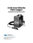
1
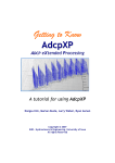
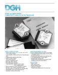
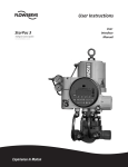
H-ADFM™
Velocity Profiler
Operation, Maintenance, & Software Manual
Part #69-7303-001 of Assembly #60-7304-004
Copyright © 2006. All rights reserved, Teledyne Isco, Inc.
Revision A, April 11, 2011
Foreword
This instruction manual is designed to help you gain a thorough understanding of the
operation of the equipment. Teledyne Isco recommends that you read this manual
completely before placing the equipment in service.
Although Teledyne Isco designs reliability into all equipment, there is always the possibility of a malfunction. This manual may help in diagnosing and repairing the malfunction.
If the problem persists, call or e-mail the Teledyne Isco Technical Service Department
for assistance. Simple difficulties can often be diagnosed over the phone.
If it is necessary to return the equipment to the factory for service, please follow the
shipping instructions provided by the Customer Service Department, including the
use of the Return Authorization Number specified. Be sure to include a note
describing the malfunction. This will aid in the prompt repair and return of the
equipment.
Teledyne Isco welcomes suggestions that would improve the information presented in
this manual or enhance the operation of the equipment itself.
Teledyne Isco is continually improving its products and reserves the right to
change product specifications, replacement parts, schematics, and instructions without notice.
Contact Information
Customer Service
Phone:
(800) 228-4373
(USA, Canada, Mexico)
(402) 464-0231
(Outside North America)
Fax:
(402) 465-3022
Email:
[email protected]
Technical Support
Phone:
Email:
(800) 775-2965
(Analytical)
(866) 298-6174
(Samplers and Flow Meters)
[email protected]
Return equipment to: 4700 Superior Street, Lincoln, NE 68504-1398
Other Correspondence
Mail to:
P.O. Box 82531, Lincoln, NE 68501-2531
Email:
[email protected]
Web site:
www.isco.com
Revised March 17, 2009
H-ADFM™ Velocity Profiler
Notes
H-ADFM™ Velocity Profiler
Notes
About this manual:
DANGER
DANGER – limited to the most extreme situations
to identify an imminent hazard, which if not
avoided, will result in death or serious injury.
WARNING
Warnings identify a potentially hazardous condition, which
if not avoided, could result in death or serious injury.
CAUTION
Cautions identify a potential hazard, which if not avoided, may
result in minor or moderate injury. This category can also warn
you of unsafe practices, or conditions that may cause property
damage.
Note
Notes contain useful information that may help you in deciding
which settings to choose.
iii
H-ADFM™ Velocity Profiler
Notes
iv
H-ADFM™ Velocity Profiler
Table of Contents
Section 1 Introduction
1.1 System Overview. . . . . . . . . . . . . . . . . . . . . . . . . . . . . . . . . . . . . . . . . . . . . . . . . . . .
1.1.1 ChannelMaster H-ADCP . . . . . . . . . . . . . . . . . . . . . . . . . . . . . . . . . . . . . . . .
1.1.2 H-ADFM Flow Computer . . . . . . . . . . . . . . . . . . . . . . . . . . . . . . . . . . . . . . .
1.1.3 WinHADFM . . . . . . . . . . . . . . . . . . . . . . . . . . . . . . . . . . . . . . . . . . . . . . . . . .
1.2 Installation Overview . . . . . . . . . . . . . . . . . . . . . . . . . . . . . . . . . . . . . . . . . . . . . . . .
1-1
1-1
1-1
1-2
1-2
Section 2 Physical Installation
2.1 ChannelMaster Installation . . . . . . . . . . . . . . . . . . . . . . . . . . . . . . . . . . . . . . . . . . . 2-1
2.2 Flow Computer Installation . . . . . . . . . . . . . . . . . . . . . . . . . . . . . . . . . . . . . . . . . . . 2-1
Section 3 Wiring Installation
3.1
3.2
3.3
3.4
3.5
ChannelMaster I/O Cable . . . . . . . . . . . . . . . . . . . . . . . . . . . . . . . . . . . . . . . . . . . . .
Power Supply. . . . . . . . . . . . . . . . . . . . . . . . . . . . . . . . . . . . . . . . . . . . . . . . . . . . . . .
Analog Data Output . . . . . . . . . . . . . . . . . . . . . . . . . . . . . . . . . . . . . . . . . . . . . . . . .
Totalizer Pulse Output . . . . . . . . . . . . . . . . . . . . . . . . . . . . . . . . . . . . . . . . . . . . . . .
Communications . . . . . . . . . . . . . . . . . . . . . . . . . . . . . . . . . . . . . . . . . . . . . . . . . . . .
3.5.1 RS-232 . . . . . . . . . . . . . . . . . . . . . . . . . . . . . . . . . . . . . . . . . . . . . . . . . . . . . .
3.5.2 RS-422 . . . . . . . . . . . . . . . . . . . . . . . . . . . . . . . . . . . . . . . . . . . . . . . . . . . . . .
3-1
3-1
3-1
3-2
3-2
3-2
3-2
Section 4 Software Installation and Station File Configuration
4.1 Introduction . . . . . . . . . . . . . . . . . . . . . . . . . . . . . . . . . . . . . . . . . . . . . . . . . . . . . . . . 4-1
4.2 Installing the Software . . . . . . . . . . . . . . . . . . . . . . . . . . . . . . . . . . . . . . . . . . . . . . . 4-1
4.3 Configuring the System Settings . . . . . . . . . . . . . . . . . . . . . . . . . . . . . . . . . . . . . . . 4-2
4.3.1 Site . . . . . . . . . . . . . . . . . . . . . . . . . . . . . . . . . . . . . . . . . . . . . . . . . . . . . . . . . 4-2
4.3.2 Display Units . . . . . . . . . . . . . . . . . . . . . . . . . . . . . . . . . . . . . . . . . . . . . . . . . 4-2
4.3.3 4-20 mA Output . . . . . . . . . . . . . . . . . . . . . . . . . . . . . . . . . . . . . . . . . . . . . . . 4-3
4.3.4 Totalizer . . . . . . . . . . . . . . . . . . . . . . . . . . . . . . . . . . . . . . . . . . . . . . . . . . . . . 4-3
4.3.5 Communications . . . . . . . . . . . . . . . . . . . . . . . . . . . . . . . . . . . . . . . . . . . . . . 4-4
4.3.6 Graphic Preferences . . . . . . . . . . . . . . . . . . . . . . . . . . . . . . . . . . . . . . . . . . . . 4-4
4.3.7 Flow Computer Settings . . . . . . . . . . . . . . . . . . . . . . . . . . . . . . . . . . . . . . . . 4-4
4.3.8 Calculation Settings . . . . . . . . . . . . . . . . . . . . . . . . . . . . . . . . . . . . . . . . . . . 4-5
4.4 Configuring the Channel Dimensions . . . . . . . . . . . . . . . . . . . . . . . . . . . . . . . . . . . 4-5
4.4.1 Mounting Orientation . . . . . . . . . . . . . . . . . . . . . . . . . . . . . . . . . . . . . . . . . . 4-6
4.4.2 Rectangular Channels . . . . . . . . . . . . . . . . . . . . . . . . . . . . . . . . . . . . . . . . . . 4-6
4.4.3 Circular Channels . . . . . . . . . . . . . . . . . . . . . . . . . . . . . . . . . . . . . . . . . . . . . 4-7
4.4.4 Trapezoidal Channels . . . . . . . . . . . . . . . . . . . . . . . . . . . . . . . . . . . . . . . . . . 4-8
4.4.5 Multi-Point Channels . . . . . . . . . . . . . . . . . . . . . . . . . . . . . . . . . . . . . . . . . . 4-9
4.4.6 Polynomial Channel . . . . . . . . . . . . . . . . . . . . . . . . . . . . . . . . . . . . . . . . . . 4-10
4.5 Configuring the Velocity Model . . . . . . . . . . . . . . . . . . . . . . . . . . . . . . . . . . . . . . . 4-10
4.5.1 Linear Regression Model . . . . . . . . . . . . . . . . . . . . . . . . . . . . . . . . . . . . . . . 4-11
4.5.2 Power-Law Regression Model . . . . . . . . . . . . . . . . . . . . . . . . . . . . . . . . . . . 4-12
4.5.3 Compound Linear-Regression Model . . . . . . . . . . . . . . . . . . . . . . . . . . . . . 4-12
4.5.4 Forced Depth . . . . . . . . . . . . . . . . . . . . . . . . . . . . . . . . . . . . . . . . . . . . . . . . 4-13
4.5.5 Profiling . . . . . . . . . . . . . . . . . . . . . . . . . . . . . . . . . . . . . . . . . . . . . . . . . . . . 4-13
v
H-ADFM™ Velocity Profiler
Table of Contents
4.5.6 Velocity Range . . . . . . . . . . . . . . . . . . . . . . . . . . . . . . . . . . . . . . . . . . . . . . . 4-14
Section 5 Programming and Testing the H-ADFM
5.1
5.2
5.3
5.4
5.5
Overview . . . . . . . . . . . . . . . . . . . . . . . . . . . . . . . . . . . . . . . . . . . . . . . . . . . . . . . . . .
Connecting the H-ADFM Flow Computer to a PC . . . . . . . . . . . . . . . . . . . . . . . . .
Verifying the DGH Module Calibration . . . . . . . . . . . . . . . . . . . . . . . . . . . . . . . . . .
Programming the Flow Computer . . . . . . . . . . . . . . . . . . . . . . . . . . . . . . . . . . . . . .
Programming the ChannelMaster . . . . . . . . . . . . . . . . . . . . . . . . . . . . . . . . . . . . . .
5.5.1 Wakeup . . . . . . . . . . . . . . . . . . . . . . . . . . . . . . . . . . . . . . . . . . . . . . . . . . . . . .
5.5.2 System Test . . . . . . . . . . . . . . . . . . . . . . . . . . . . . . . . . . . . . . . . . . . . . . . . . .
5.5.3 Zero Pressure . . . . . . . . . . . . . . . . . . . . . . . . . . . . . . . . . . . . . . . . . . . . . . . . .
5.5.4 Check Orientation . . . . . . . . . . . . . . . . . . . . . . . . . . . . . . . . . . . . . . . . . . . . .
5.5.5 Download Data . . . . . . . . . . . . . . . . . . . . . . . . . . . . . . . . . . . . . . . . . . . . . . . .
5.5.6 Erase Data . . . . . . . . . . . . . . . . . . . . . . . . . . . . . . . . . . . . . . . . . . . . . . . . . . .
5.5.7 Set Time . . . . . . . . . . . . . . . . . . . . . . . . . . . . . . . . . . . . . . . . . . . . . . . . . . . . .
5.5.8 Sleep . . . . . . . . . . . . . . . . . . . . . . . . . . . . . . . . . . . . . . . . . . . . . . . . . . . . . . . .
5.5.9 Program . . . . . . . . . . . . . . . . . . . . . . . . . . . . . . . . . . . . . . . . . . . . . . . . . . . . .
5.6 Listen Realtime . . . . . . . . . . . . . . . . . . . . . . . . . . . . . . . . . . . . . . . . . . . . . . . . . . . . .
5-1
5-1
5-1
5-3
5-4
5-4
5-4
5-5
5-5
5-5
5-6
5-6
5-7
5-7
5-7
Section 6 Reviewing Collected Data
6.1 Refresh . . . . . . . . . . . . . . . . . . . . . . . . . . . . . . . . . . . . . . . . . . . . . . . . . . . . . . . . . . . .
6.2 View Data . . . . . . . . . . . . . . . . . . . . . . . . . . . . . . . . . . . . . . . . . . . . . . . . . . . . . . . . .
6.2.1 Configuring the Data Display . . . . . . . . . . . . . . . . . . . . . . . . . . . . . . . . . . . .
6.2.2 Resizing Display Areas . . . . . . . . . . . . . . . . . . . . . . . . . . . . . . . . . . . . . . . . .
6.2.3 Hydrograph . . . . . . . . . . . . . . . . . . . . . . . . . . . . . . . . . . . . . . . . . . . . . . . . . .
6.2.4 Velocity Distribution Whisker Graph . . . . . . . . . . . . . . . . . . . . . . . . . . . . . .
6.2.5 Beam Graphs . . . . . . . . . . . . . . . . . . . . . . . . . . . . . . . . . . . . . . . . . . . . . . . . .
6.2.6 Tabular Display . . . . . . . . . . . . . . . . . . . . . . . . . . . . . . . . . . . . . . . . . . . . . . .
6-1
6-1
6-1
6-1
6-2
6-3
6-3
6-4
Appendix A Current Loop Calibration
List of Figures
1-1
3-1
3-2
4-1
4-2
4-3
4-4
5-1
5-2
5-3
6-1
H-ADFM Flow Computer . . . . . . . . . . . . . . . . . . . . . . . . . . . . . . . . . . . . . . . . . . . . . 1-2
Analog Output Terminal Block . . . . . . . . . . . . . . . . . . . . . . . . . . . . . . . . . . . . . . . . 3-2
RS-422 Configuration . . . . . . . . . . . . . . . . . . . . . . . . . . . . . . . . . . . . . . . . . . . . . . . . 3-2
Channel Dimensions . . . . . . . . . . . . . . . . . . . . . . . . . . . . . . . . . . . . . . . . . . . . . . . . 4-6
Linear Regression Model . . . . . . . . . . . . . . . . . . . . . . . . . . . . . . . . . . . . . . . . . . . . 4-11
Power-Law Regression Model . . . . . . . . . . . . . . . . . . . . . . . . . . . . . . . . . . . . . . . . 4-12
Compound Linear-Regression Model . . . . . . . . . . . . . . . . . . . . . . . . . . . . . . . . . . 4-13
Connecting the H-ADFM to a PC . . . . . . . . . . . . . . . . . . . . . . . . . . . . . . . . . . . . . . 5-1
DGH Test Settings . . . . . . . . . . . . . . . . . . . . . . . . . . . . . . . . . . . . . . . . . . . . . . . . . . 5-2
Listen Realtime data window . . . . . . . . . . . . . . . . . . . . . . . . . . . . . . . . . . . . . . . . . 5-8
Data display . . . . . . . . . . . . . . . . . . . . . . . . . . . . . . . . . . . . . . . . . . . . . . . . . . . . . . . 6-3
List of Tables
4-1
4-2
4-3
4-4
vi
User-Selectable Units of Measure . . . . . . . . . . . . . . . . . . . . . . . . . . . . . . . . . . . . . .
Rectangular Channel Fields . . . . . . . . . . . . . . . . . . . . . . . . . . . . . . . . . . . . . . . . . .
Circular Channel Fields . . . . . . . . . . . . . . . . . . . . . . . . . . . . . . . . . . . . . . . . . . . . . .
Trapezoidal Channel Fields . . . . . . . . . . . . . . . . . . . . . . . . . . . . . . . . . . . . . . . . . . .
4-3
4-7
4-8
4-9
H-ADFM™ Velocity Profiler
Table of Contents
4-5
5-1
A-1
A-2
Velocity Model Variables . . . . . . . . . . . . . . . . . . . . . . . . . . . . . . . . . . . . . . . . . . . . 4-10
DIP Switch (SW2) Settings for DGH Verification . . . . . . . . . . . . . . . . . . . . . . . . . 5-2
DIP Switch (SW2) Settings for DGH Calibration . . . . . . . . . . . . . . . . . . . . . . . . . A-1
SW2 DIP Switch Functions . . . . . . . . . . . . . . . . . . . . . . . . . . . . . . . . . . . . . . . . . . . A-1
vii
H-ADFM™ Velocity Profiler
Table of Contents
viii
H-ADFM™ Velocity Profiler
Section 1 Introduction
1.1 System Overview
The Horizontal Acoustic Doppler Flow Meter (H-ADFM) from
Teledyne Isco, Inc. leverages the exceptional velocity profiling
capability of the ChannelMaster horizontal ADCP manufactured
by Teledyne RDI, Inc. The H-ADFM system consists of the ChannelMaster instrument and an Isco-designed Flow Computer that
accurately measure depth and velocity and calculate flow rates.
Each component is described in more detail below.
1.1.1 ChannelMaster
H-ADCP
The H-ADFM is a Horizontal Acoustic Doppler Current Profiler
(H-ADCP). It is available in 300kHz, 600kHz, and 1200kHz configurations. The instrument houses three transducers: two for
velocity measurement and one for water depth measurement. It
also houses pressure, temperature, and pitch and roll sensors.
The pitch and roll sensors are used to ensure that the instrument
is installed in the correct orientation, as this is crucial for proper
operation. The ChannelMaster measures velocity vectors at
various points along its velocity beam axis along with the range
to the water surface, and transmits that data to the Flow Computer.
1.1.2 Software
The
WinHADFM
1.2 Installation Overview
Teledyne Isco recommends installing the H-ADFM system in the
following order:
1. Physical installation
2. Wiring installation
3. Station file configuration
4. Programming and testing
1-1
H-ADFM™ Velocity Profiler
Section 1 Introduction
1-2
H-ADFM™ Velocity Profiler
Section 2 Physical Installation
Physical installation of the H-ADFM consists of installing the
ChannelMaster in the channel to be measured and installing the
Flow Computer nearby.
2.1 ChannelMaster
Installation
For instructions on how to mount the ChannelMaster, refer to the
ChannelMaster Quick Start Guide and/or the ChannelMaster
Operation Manual provided with the ChannelMaster documentation.
Note
Proper orientation (pitch, roll, and heading) of the ChannelMaster is essential for reliable ChannelMaster operation. WinHADFM provides a function for checking the pitch and roll of
the ChannelMaster. See Section 5 for more details.
2.2 Flow Computer
Installation
The specific arrangement of components in an H-ADFM flow
monitoring system can vary greatly, and depends to a large
extent on the physical parameters of the monitoring location.
However, the distance between the Flow Computer and the
ChannelMaster is significant because the standard ChannelMaster I/O cable is 75 feet long. If the ChannelMaster and the
Flow Computer are more than 75 feet apart, RS-422 communication should be used and additional user-supplied wiring will be
required.
A minimum clearance of two inches (50mm) should be provided
on the top and on both sides of the Flow Computer, with the
minimum clearance increased to six inches (150 mm) on the
bottom of the enclosure to provide access for cable entry. The
enclosure may be installed in any orientation; however, readability of the display will suffer if the enclosure is not oriented
vertically.
The Flow Computer is packaged in a NEMA 4X enclosure with
power supply and terminal strips for field wiring connections.
2-1
H-ADFM™ Velocity Profiler
Section 2 Physical Installation
2-2
H-ADFM™ Velocity Profiler
Section 3 Wiring Installation
All field wiring connections to the ChannelMaster H-ADCP are
made using the supplied I/O cable. Field wiring to the Flow Computer is connected to the terminal block marked TB2. Each
position within TB2 is marked with its function rather than a
terminal number, for ease of connection in the field.
3.1 ChannelMaster I/O
Cable
The ChannelMaster I/O cable provides both power and communications connections to the ChannelMaster through a single
underwater-style rubberized connector. Power supply and communications functions are broken out at the other end of the
cable into separate cables using molded “Y” junctions. The power
supply cable terminates in individual DC+ and DC– wires with
alligator clamps for quick connection to a 12V battery. The communications cable is terminated in a standard 9-pin Female
D-sub connector. The same I/O cable is used for both RS-232 and
RS-422 communications.
3.2 Power Supply
The H-ADFM (ChannelMaster and Flow Computer) requires +10
to +18 VDC, unregulated, for full operation. Typical power consumption will be approximately 4.5 watts (370 mA at 12VDC).
Connect the ChannelMaster DC power supply leads to the DC
power supply or batteries. Teledyne Isco suggests cutting off the
alligator clamps and hard-wiring the I/O cable power supply
leads to the DC power source for better reliability in permanent
or semi-permanent applications. Also connect DC power to the
DC power supply terminals (or to the J6 connector), marked DC+
and DC–, on the Flow Computer.
3.3 Analog Data Output
The H-ADFM Flow Computer can be equipped with up to three
independent analog channels, each capable of driving up to a 600
ohm load. Analog outputs on these channels are generated using
DGH Corporation Model 3251 current output modules. These
modules act as 4-wire transmitters (i.e. the DGH module provides power to the analog loop). Each analog output is electrically
isolated from the remainder of the Flow Computer circuitry.
Analog output channels are designated as Flow (QA+, QA–),
Depth (DA+, DA–), and Velocity (VA+, VA–). Connect each analog
output channel to the appropriate external loads/devices, consistent with standard current loop wiring practices for 4-wire
transmitters, and ensure that the total load for each loop does
not exceed 600 ohms.
3-1
H-ADFM™ Velocity Profiler
Section 3 Wiring Installation
Figure 3-1 Analog Output Terminal Block
3.4 Totalizer Pulse Output
The H-ADFM Flow Computer computes incremental volume and
outputs digital pulses based on a user-specified volume
increment. The totalized volume is also displayed on the LCD
screen and is reset with each power cycle or when the unit
receives new settings. The pulse outputs can be connected to an
external device to keep track of totalized output over multiple
power cycles. Pulse outputs are available as either +5VDC pulses
(P5+, P5–) or as dry contact closures (NO, COMM). The +5VDC
pulse, if used, can source a maximum current of 15mA. Dry
contact closures are provided by a solid-state relay rated at
3-60VDC, 0.02 - 1.0 amps.
3.5 Communications
3.5.1 RS-232
H-ADFM Flow Computers configured for RS-232 communication
will include a short RS-232 cable extending from the J1 terminal
inside the Flow Computer enclosure. This cable terminates in a
9-pin male D-sub connector. The ChannelMaster communications cable connects directly to this connector.
3.5.2 RS-422
H-ADFM Flow Computers configured for RS-422 communication
will include an RS-232 to RS-422 converter inside the Flow Computer enclosure, as shown in Figure 3-2.
Figure 3-2 RS-422 Configuration
3-2
H-ADFM™ Velocity Profiler
Section 3 Wiring Installation
A short cable will extend from the RS-422 side of the converter to
the exterior of the Flow Computer enclosure. This cable will terminate in a 9-pin male D-sub connector. The ChannelMaster
communications cable connects directly to this connector.
3-3
H-ADFM™ Velocity Profiler
Section 3 Wiring Installation
3-4
H-ADFM™ Velocity Profiler
Section 4 Software Installation and Station File
Configuration
4.1 Introduction
WinHADFM is the primary program used to configure and
operate an H-ADFM system. System configuration information is
saved in a station file (*.hstn). Station files may (optionally) be
grouped as desired. The station file is also used to display collected data. Station files, and associated data files, are stored in
the following directory path:
C:\WinHADFM\SITES\<groupname>\<stationname>
WinHADFM will automatically scan this path for valid station
files and display a list of stations sorted by group each time the
program is started.
Note
WinHADFM will automatically select and display information
for the first station in the station file list when the program is
started. Ensure that you select the desired station file before
entering configuration changes or programming the Flow Computer and ChannelMaster.
Two other software programs may at times be required:
• DGH Utility software is used to configure and test the
analog output signal generator modules incorporated
into the Flow Computer. Installation of this program is
strongly recommended.
• The Basic-X download utility is used to flash updated
firmware into the Flow Computer. Installation of this
program is optional and only required if updated
firmware for the Flow Computer becomes available.
4.2 Installing the Software
Before configuring the H-ADFM station file, you must install
Win-HADFM and the DGH Utility Software 2000. These programs will run on computers with Windows 95 and newer operating systems.
Note
The Basic-X Download Utility will also be required if updates to
the firmware in the Flow Computer are required.
Installing WinHADFM – To i n s t a l l Wi n - H A D F M , s i m p l y
double-click the WinHADFM Setup program and follow the
installer's prompts.
4-1
H-ADFM™ Velocity Profiler
Section 4 Software Installation and Station File Configuration
Installing the DGH Utility Software 2000 – To i n s t a l l t h e
DGH Utility Software 2000 setup file, simply double-click the
Setup program and follow the installer’s prompts. The version
currently distributed with the H-ADFM is V2_0_2_1.
Installing the Basic-X Download Utility software – To
install the Basic-X Download Utility software simply double click
the Basic-X setup program and follow the installer’s prompts.
The version currently distributed with the H-ADFM is V2_10.
4.3 Configuring the
System Settings
To create a new station file, click the new station icon in the
upper left corner of the Win-HADFM window. You will now have
a configuration window divided into three tabs: System,
Channel, and Velocity Model. The system tab window is divided
into the following seven sections:
• Site
• Display Units
• 4-20 Output
• Totalizer
• Communications
• Graphics Preferences
• Flow Computer Settings
4.3.1 Site
The Site section contains information about the installation site.
Multiple configurations can be saved and used later. Sites can
also be arranged in groups.
Site Name – Enter the name of the specific installation site.
Group – Enter the name of the group that this site belongs to. A
group name is not necessary.
Location – Enter the physical location of the site.
4.3.2 Display Units
The Display Units section contains pull-down menus for flow,
velocity, stage, volume, and temperature. The unit types you set
here determine not only the units displayed on the LCD display
of the Flow Computer, but also the units used to set the analog
output spans, the Totalizer Pulse increments, and the channel
dimensions. The unit indicators next to the input fields for these
parameters will change to reflect your choices in the unit
window.
The units selected for stage also determine the units for the
channel dimensions in the Channel tab. Selecting an English
measurement (e.g. inches) for stage will require the channel to be
dimensioned in English units (inches). Selecting a metric measurement (e.g. meters) will require you to dimension the channel
in metric units (meters).
Note
If the unit selected for stage is modified after channel dimensions have been entered, those dimensions will be re-scaled
accordingly.
4-2
H-ADFM™ Velocity Profiler
Section 4 Software Installation and Station File Configuration
Table 4-1 lists the units available for each measurement.
Table 4-1 User-Selectable Units of Measure
Measurement
Available Units
Flow
MGD, Gallons per minute, Cubic meters per second, Liters per second, Cubic
feet per second, Million liters per day
Velocity
Meters per second, Feet per second, Millimeters per second, Centimeters per
second
Stage
Inches, Centimeters, Millimeters, Meters
Volume
Liters, Cubic meters, Megaliters, Gallons, Cubic feet, KGallons, Million Gallons, Acre Feet
Temperature
Degrees Fahrenheit, Degrees Celsius
4.3.3 4-20 mA Output
The 4-20 Output section of the System tab allows you to set the
relationship between the digital and analog signals of the Flow
Computer. The Flow Computer generates an analog signal that
ranges from 4mA to 20mA Therefore, a signal of 4mA will represent the low-limit of the H-ADFM's analog output and a 20mA
signal will represent the high-limit of that output. Values
between these limits are determined by linear interpolation.
For example, if you set the low limit for flow at zero GPM
(outputs 4mA) and the high limit at 500GPM (outputs 20mA),
then a 250GPM flow will result in an analog signal of 12mA
[250/500(20-4)+4]. The resolution of this analog representation of
the digital data is .01mA.
Note
Ensure adequate margins when setting the high/low limits; otherwise, data will be clipped. This can happen because measurements from the Flow Computer that are less than the
specified low-limit will result in an analog output of 4mA, and
values that exceed the high-limit will result in a 20mA output.
There is no indication that the measurements have exceeded
the limits, resulting in ambiguous data.
Note
In the case of bad or missing velocity or stage data from the
ChannelMaster, the H-ADFM Flow Computer will output a specific user-defined signal level: by default, 3.9 mA for bad data,
or 3.6 mA when no data is received from the ChannelMaster.
However, these output values do not apply to clipped data
(data that exceeds the high/low-limits set in the span section).
4.3.4 Totalizer
The Flow Computer is capable of sending out a pulse of
user-defined length (50 milliseconds by default), when the measured volume increases by the amount specified in the Totalizer
Pulse field. The units for this value are the same as the units
specified for Volume in the Units section.
4-3
H-ADFM™ Velocity Profiler
Section 4 Software Installation and Station File Configuration
Note
The built-in totalizer uses volatile memory and will reset to zero
when power is disconnected or when new configuration settings are sent to the Flow Computer.
Note
Setting the Totalizer Pulse value too small will cause the Flow
Computer to stop responding to data from the ChannelMaster.
4.3.5 Communications
The Communications drop-down list allows you to select the Com
port your computer uses for its serial connection.
4.3.6 Graphic Preferences
Click the Graphics Preferences button to bring up a new dialog
box where you can specify which graphs and data types to
display when viewing data.
4.3.7 Flow Computer
Settings
Click the Flow Computer Settings button to bring up a new
dialog box where you can specify what analog value(s) to output
in the case of bad or missing data, how many consecutive bad
readings are allowed before the flow computer switches to the
appropriate analog output value(s), how long the flow computer
will wait for data from the ChannelMaster before timing out, the
duration of the totalizer pulse, and what smoothing parameters
(if any) are used for data display and output.
Smoothing
Smoothing multiplies a portion of the current reading by the previous reading:
R = TCF * M + (1 - TCF) * P
where:
M is the current measured value from the instrument.
P is the previous output value.
R is the new output data value.
Note that R becomes the P for the next reading. Also, a TCF of
1.0 means that no smoothing will be performed (this is the
default). The smoothing time constant (TC) is calculated from the
TCF and sample interval, and is displayed for the user’s information.
4-4
Big Step
The Flow Computer is designed to respond quickly when large
changes in flow rate occur rapidly. The smoothing specified by
the TCF value is ignored and the new output data value equals
the current measured output when the change in flow rate
exceeds the specified percentage of the analog output span. The
Big Step value is that percentage, entered as a decimal fraction
of the analog output span for flow rate. The corresponding flow
rate change is displayed for the user’s information.
Zero Screen
All instruments become less precise when reading values very
near to zero. The Flow Computer is designed to output a zero
reading when the flow rate is very low. The Zero Screen value is
H-ADFM™ Velocity Profiler
Section 4 Software Installation and Station File Configuration
the user-selected percentage, entered as a decimal, of the analog
output span for flow rate below which the output will always be
forced to zero.
4.3.8 Calculation Settings
Calculated flow rates are not stored in H-ADFM download data
files. Flow data displayed in the WinHADFM software is re-calculated each time it is displayed. This dialog box displays the
geometry and velocity model settings in effect at various times.
New entries in this table are created automatically each time the
Flow Computer is programmed. Entries can be created, modified,
or removed as desired by the user to evaluate the effects of
changes to the geometry and velocity models on flow calculation.
Changes to these settings will normally be made only by experienced users.
Note
Calculation setting entries store the channel geometry settings
in effect at the time the entry was created. Channel geometry
settings cannot be edited once created. If you wish to change
the channel geometry settings in use for a given time period,
you must configure the station file for the desired geometry
settings, create the calculation settings entry, then (if necessary) return the geometry settings to their correct values.
Note
Calculation settings are currently not sorted by date/time. The
user must ensure that all calculation setting entries are
arranged in proper date/time sequence.
4.4 Configuring the
Channel Dimensions
Use the Channel tab to specify the channel cross-section dimensions used in the flow calculations. The Channel tab consists of a
display window that shows a graphic representation of the
channel cross-section you define, as well as input fields for the
channel type and the specific dimensional inputs required for
each type. Five types of channel-dimensioning schemes can be
used:
• Rectangular channels
• Circular channels
• Trapezoidal channels
• Multi-Point channels
• Polynomial
4-5
H-ADFM™ Velocity Profiler
Section 4 Software Installation and Station File Configuration
Y_ADCP
Figure 4-1 Channel Dimensions
4.4.1 Mounting Orientation
The mounting orientation specifies which side of the channel the
instrument is mounted on with respect to the flow direction. The
screen view of flow faces downstream. WinHADFM software and
the H-ADFM follow the USGS convention of looking downstream
to determine which side of the channel is the left bank and which
is the right bank. Top and Bottom mounting orientations assume
that the ChannelMaster is installed with beam 1 facing
upstream (into the flow).
4.4.2 Rectangular Channels
The Rectangular Channel scheme allows you to define a simple
rectangular channel by entering values for the bottom width and
the height. Entries are required for mounting orientation,
Y-ADCP, Z-ADCP, and Z-Bottom. Y-ADCP is the distance
between the ChannelMaster and the wall of the channel.
Z-ADCP is the height of the ChannelMaster depth beam ceramic
above the reference datum. Z-Bottom is the height of the channel
bottom above the reference datum. Therefore, if the channel
bottom is used as the reference datum, the Z-Bottom value will
be zero.
The mounting orientation specifies which side of the channel the
instrument is mounted on with respect to the flow direction.
Flow direction in the graphic window is away from you, into the
screen.
Table 4-2 describes the fields used to define a rectangular
channel.
4-6
H-ADFM™ Velocity Profiler
Section 4 Software Installation and Station File Configuration
Table 4-2 Rectangular Channel Fields
Field
Description
Z-ADCP
Z-ADCP is the height (in units selected for stage in the System tab) of
the H-ADFM above the reference datum. This value is determined
when the H-ADFM is installed and configured. Z-ADCP is marked by a
blue line in the display window.
Reference Datum
The reference datum is a user-specified line located at or below the
channel bottom. The reference datum is always Z = zero for the coordinate system used to define the channel cross section, regardless of
where it is at in relation to the channel.
Z-Bottom
Z-Bottom is the distance between the reference datum and the bottom
of the channel. This value is zero if the channel bottom and the reference datum are the same (i.e. Z = zero).
Width
The Width is the width of the channel at depth = Z-Bottom. Use the
units shown below the channel-drawing window.
Y-ADCP
The distance between the ChannelMaster and the wall of the Channel.
This is used by the ChannelMaster to calculate the distance across the
channel at the instrument mounting height.
Height
Height is the distance from the top of the channel to the reference
datum. This is an absolute value because it is referenced to the local
coordinate system. Therefore, if your reference datum is 5 feet below
the channel bottom (i.e. Z-Bottom = 5), and the channel is 10 feet deep,
the Height would be 15 feet. See Figure 4-1 for further clarification.
Mounting Orientation
Determines the orientation of the ChannelMaster with respect to the
flow direction (into the screen). If the orientation is not specified correctly, velocity values will be reversed.
4.4.3 Circular Channels
The circular channel scheme allows you to define a simple circular channel by entering values for the diameter and Z-ADCP.
Note
Care must be taken when installing the ChannelMaster in a circular channel to ensure that the ultrasonic depth sensor
(up-looking beam) can properly measure water depth.
Depending on the installation, the curved wall above the ChannelMaster may interfere with this measurement.
Table 4-3 describes the fields used to define a circular channel.
4-7
H-ADFM™ Velocity Profiler
Section 4 Software Installation and Station File Configuration
Table 4-3 Circular Channel Fields
Field
Description
Z-ADCP
Z-ADCP is the height (in units selected for stage in the System tab) of
the H-ADFM above the reference datum. This value is determined when
the H-ADFM is installed and configured. Z-ADCP is marked by a blue
line in the display window.
Reference Datum
The reference datum is a user-specified line located at or below the
channel bottom. The reference datum is always Z = zero for the coordinate system used to define the channel cross section, regardless of
where it is at in relation to the channel.
Diameter
Diameter is the diameter of the circular channel, set in the units specified in the System tab.
Y-ADCP
The distance between the ChannelMaster and the wall of the Channel.
This is used by the ChannelMaster to calculate bin positions across the
channel at instrument height.
Mounting Orientation
Determines the orientation of the ChannelMaster with respect to the
flow direction (into the screen). If the orientation is not specified correctly, negative velocity values will be recorded.
4.4.4 Trapezoidal Channels
Use the Trapezoidal scheme for channels with sloping sides.
Values must be entered for the Height, Bottom Width, and
sidewall slope. The sidewall slope (rise/run) is unit-less and
cannot be set to zero. Z-Bottom specifies the height of the
channel bottom above the reference datum. Therefore, if the reference datum is located at the channel bottom, the Z-Bottom
value will be zero.
Note
The Height and Width-Bottom fields are not measured in similar ways. The Height dimension is the distance between the
top of the channel and the reference datum. The Width-Bottom
dimension is the actual width of the channel bottom.
The subtle difference here is that the Height is referenced to
the origin of the local coordinate system (Z = zero), making it
an absolute dimension. Width-Bottom, on the other hand, is
not referenced to the origin, making it a relative dimension.
Table 4-4 describes the fields used to define a trapezoidal
channel.
4-8
H-ADFM™ Velocity Profiler
Section 4 Software Installation and Station File Configuration
Table 4-4 Trapezoidal Channel Fields
Field
Description
Z-ADCP
Z-ADCP is the height (in units selected for stage in the System tab) of
the H-ADFM above the reference datum. This value is determined
when the H-ADFM is installed and configured. Z-ADCP is marked by a
blue line in the display window.
Reference Datum
The reference datum is a user-specified line located at or below the
channel bottom. The reference datum is always Z = zero for the coordinate system used to define the channel cross section, regardless of
where it is at in relation to the channel.
Z-Bottom
Z-Bottom is the distance between the reference datum and the bottom
of the channel. This value is zero if the channel bottom and the reference datum are the same (i.e. Z = zero).
Width
The Width is the width of the channel bottom. Use the units shown
below the channel-drawing window. Unlike the Height value, the
Width-Bottom value is not in reference to the local coordinate system.
Y-ADCP
The distance between the ChannelMaster and the wall of the Channel.
This is used by the ChannelMaster to calculate the distance across at
instrument height.
Height
Height is the distance from the top of the channel to the reference
datum. This is an absolute coordinate because it is referenced to the
local coordinate system. Therefore, if your reference datum is 5 feet
below the channel bottom (i.e. Z-Bottom = 5), and the channel is 10 feet
deep, the Height would be 15 feet. See Figure %% for further clarification.
Mounting Orientation
Determines the orientation of the ChannelMaster with respect to the
flow direction (into the screen). If the orientation is not specified correctly, negative velocity values will be recorded.
Slope
Slope is the inclination of the channel walls. It is specified as a ratio
(rise over run) and cannot be set to zero. This value is dimensionless.
4.4.5 Multi-Point Channels
This option allows you to specify a channel shape as a series of Y,
Z coordinates. Y refers to the horizontal dimension and Z refers
to the vertical dimension relative to the reference datum. When
entering the coordinates, the following rules must be followed:
• Each Y value must be greater than the Y value that
precedes it, so that the points are arranged in order left
to right. The first Y value should be zero (the left bank of
the channel should be used as the Y axis reference
point).
• Side channels are not allowed (see below).
• The channel must slope downwards to a minimum Z
value, and then slope back upwards. It is acceptable, but
not required, to use zero as the minimum Z value.
• The final Z value should equal the first Z value.
4-9
H-ADFM™ Velocity Profiler
Section 4 Software Installation and Station File Configuration
4.4.6 Polynomial Channel
Cross-sectional area of a channel can be defined as a function of
water depth by a polynomial equation as follows:
Area = A1 + A2*H + A3 * H2
where:
H = Water depth relative to the reference datum Z = 0
A1, A2, A3 = polynomial coefficients
Please consult Teledyne Isco if you wish to use the Polynomial
Channel and require assistance in developing a polynomial
channel model.
4.5 Configuring the
Velocity Model
Channel configurations and velocity profile distributions in
channels where the H-ADFM will typically be used will be much
more variable than channels where a standard vertically oriented ADFM would be used. The H-ADFM uses an Index Velocity
and a Velocity Model to calculate flow rates from channel
geometry, stage, and velocity profile information. Accuracy of an
H-ADFM system can only be assured if suitable calibration measurements are taken and used to develop a site-specific velocity
model. Calibration measurements and the velocity model should
span the entire range of stage and velocity conditions experienced at the site for greatest flow measurement reliability.
The ChannelMaster Index Velocity Vi is a straight (not weighted)
average of the individual velocities for each bin in the specified
index range.
WinHADFM and the H-ADFM Flow Computer have three
velocity models to choose from: Linear Regression, Power-Law
Regression, and Compound Linear Regression. The selected
model is used to calculate the average velocity and flow rate from
the index velocity.
The following variables are used in the velocity models:
Table 4-5 Velocity Model Variables
4-10
Variable
Description
V=
The final computed average velocity.
Vi=
The index velocity, computed as an average of the velocity bins specified in
the Index Range fields.
Vc=
The critical velocity used in the Compound Linear Regression velocity model.
When this average velocity is reached or exceeded, the second equation in
the model is used.
H=
The stage, or water height, in the units specified in the Units section of the
System tab. See Figure 4-1 for more information.
A,Bn=
Any user-designed coefficient used in the velocity calculation.
H-ADFM™ Velocity Profiler
Section 4 Software Installation and Station File Configuration
Note
For more information about determining the site-specific
regression coefficients, please refer to the following application
notes:
http://www.adcp.com/pdfs/channelmaster_checkpoint13.pdf
http://www.adcp.com/pdfs/channel_streampro_imperial.pdf
4.5.1 Linear Regression
Model
The Linear Regression model calculates the average velocity V at
time t. B 1, B2 , and B 3 are site-specific regression coefficients.
These will have been determined by the user using independent
calibration data when the H-ADFM was installed and configured.
In cases where the effect of stage on the velocity model is insignificant, the linear regression equation may be reduced to a
one-parameter linear regression such as V=B 1 +B 2 V I . This is
achieved by entering zero in the B3 field.
Figure 4-2 Linear Regression Model
4-11
H-ADFM™ Velocity Profiler
Section 4 Software Installation and Station File Configuration
4.5.2 Power-Law Regression
Model
The Power-Law Regression model calculates average velocity V
at time t and uses site-specific regression coefficients (a, B).
These will have been determined by the user using independent
calibration data when the H-ADFM was installed and configured.
Figure 4-3 Power-Law Regression Model
4.5.3 Compound
Linear-Regression
Model
4-12
The Compound Linear-Regression model calculates mean
velocity and is used when extreme hydraulic conditions prevent
the use of the standard linear regression model. The critical
velocity Vc determines the velocity at which the second equation
is used for velocity calculation. Vc must be set in the units specified for velocity in the Units section of the System tab.
H-ADFM™ Velocity Profiler
Section 4 Software Installation and Station File Configuration
Figure 4-4 Compound Linear-Regression Model
4.5.4 Forced Depth
Water depth (stage) measurement is not always possible in some
applications, notably in circular pipes (or other channel shapes)
which always flow full, and/or applications in which a top or
bottom mounting orientation is used. A constant stage is
assumed in these types of applications by selecting Forced Depth
and entering the desired stage (in user-defined units). The
H-ADFM will calculate area and flow rate based on the stage,
channel geometry, and measured velocity profile data.
4.5.5 Profiling
Accurate velocity profile measurement requires that several
parameters be properly programmed within the ChannelMaster.
WinHADFM has been developed to streamline and simplify the
selection of proper values for those parameters based on the
channel geometry and the settings in this section.
System Frequency – Proper settings for some velocity profiling
parameters depend on the ChannelMaster frequency of operation. Select from 1200 khz, 600 khz, or 300 khz as appropriate
for your application. WinHADFM will confirm this selection
whenever it connects to the ChannelMaster.
4-13
H-ADFM™ Velocity Profiler
Section 4 Software Installation and Station File Configuration
Sample Interval – Select the desired update interval.
Automatically Calculate Settings – Select this checkbox to
allow WinHADFM to automatically calculate velocity profiling
parameter settings.
Optimization strategy – The H-ADFM flow computer can
process data using a maximum of 30 velocity profile bins.
Velocity profile data will have the greatest precision when a
small number of larger bins are used.
Velocity profile data will have the greatest resolution and the
smallest dead zones adjacent to the ChannelMaster and the far
side of the channel when a large number of smaller bins are
used. A balance between better precision and better resolution is
obtained by using a moderate number of medium sized bins.
Select from:
• Optimize velocity precision (10 bins)
• Optimize horizontal resolution (30 bins)
• Balance precision/resolution (20 bins)
Edit Commands – Clicking this button will bring up a new
dialog box listing the commands that will be sent to the ChannelMaster when it is programmed. Teledyne Isco normally recommends using the default values generated by WinHADFM.
Please contact Teledyne Isco if you wish to override the default
command settings and require assistance or additional information.
4.5.6 Velocity Range
4-14
WinHADFM will automatically select a range of velocity profile
bins to use in calculating the index velocity V i based on the
channel geometry and the profiling settings. The bin number
range selected by the program is shown when the “Calculate
Automatically” checkbox is selected. Channel configuration,
hydraulic conditions, and/or calibration measurement results
may dictate using a different range of velocity profile bins to calculate the index velocity. Manually select the desired index
velocity bin range by deselecting the “Calculate Automatically”
checkbox and entering the desired first and last bin numbers in
the appropriate fields. The index velocity is the average velocity
for all bins in the index velocity range.
H-ADFM™ Velocity Profiler
Section 5 Programming and Testing the H-ADFM
5.1 Overview
After installing the H-ADFM and configuring a station file, you
must program and test the H-ADFM. This is done using
Win-HADFM and the DGH Utility 2000 software. Programming
and testing should be performed in the following order:
1. Verify the DGH Module calibration.
2. Program the H-ADFM Flow Computer.
3. Program the ChannelMaster.
5.2 Connecting the
H-ADFM Flow
Computer to a PC
WinHADFM and the DGH Utility software communicate with
the ChannelMaster and Flow Computer through the PC's serial
port using a standard RS-232 serial cable (9-pin M-F straight
through, not null-modem or crossover). Connect the cable to the
appropriate port P1-P5 on the Flow Computer as shown in the
photo below.
Figure 5-1 Connecting the H-ADFM to a PC
5.3 Verifying the DGH
Module Calibration
The DGH Signal Generator Modules are configured at the
factory, but it is a good idea to verify that the calibration is
correct for each installation. To perform the verification, you will
need a PC with the DGH Utility Software 2000 installed and the
appropriate serial cable. Follow the steps below to verify correct
calibration. This procedure must be performed for each of the
three output channels.
1. Plug one end of the serial cable into your PC's serial port.
Plug the other end into the connector on the Flow Com-
5-1
H-ADFM™ Velocity Profiler
Section 5 Programming and Testing the H-ADFM
puter's electronics board that corresponds to the output
channel being verified (P2-flow, P3-depth, or P4-velocity).
2. Set the DIP switches (SW2) to the following:
Table 5-1 DIP Switch (SW2) Settings for DGH Verification
Switch
Setting
1
N/A
2
On
3
N/A
4
On/Off, turn off if testing flow channel.
5
On/Off, turn off if testing depth channel.
6
On/Off, turn off if testing velocity channel.
3. Launch the DGH Utility Software 2000 program.
4. From the Tools menu, select “Evaluation Screen” then
select “D3000/D4000 Series Module.”
5. Set the parameters as shown in Figure 5-2.
Figure 5-2 DGH Test Settings
5-2
H-ADFM™ Velocity Profiler
Section 5 Programming and Testing the H-ADFM
6. Click Start.
7. Set the Analog Output Control slider to 4mA. (Clicking
beside the slider will cause it to move in increments of 4
mA.)
8. Measure the output at the receiving device (whatever the
analog output channel is connected to).
9. Repeat steps 7 and 8 as desired for other output values
between 4 and 20 mA. Repeat steps 1-8 for each additional
output channel. If required, follow the procedure provided
in Appendix A to recalibrate the DGH Module(s).
5.4 Programming the
Flow Computer
The Flow Computer is the portion of the H-ADFM system that
computes average velocity and flow rate from the depth range
and velocity profile information collection by the ChannelMaster.
The Flow Computer must be reprogrammed after all configuration changes to the WinHADFM station file (except changes to
the Graphics Preferences and Calculation Settings). This ensures
that the Flow Computer is using the correct parameters for
velocity and flow computations.
The firmware version in the Flow Computer must be compatible
with the WinHADFM software version to ensure successful programming. Mismatches between the Flow Computer firmware
and the WinHADFM software are annunciated either as messages on the Flow Computer display or as message boxes in the
WinHADFM software. The Flow Computer firmware version is
displayed briefly on its LCD display when it is powered on or
reset. Teledyne Isco recommends always upgrading to the latest
Flow Computer firmware version and WinHADFM software versions to ensure proper and reliable H-ADFM system operation.
Note
WinHADFM will automatically select and display information
for the first station in the station file list when the program is
started. Ensure that you select the desired station file before
entering configuration changes or programming the Flow Computer and ChannelMaster.
To program the flow computer:
1. Set DIP switch SW2-3 to the OFF position. This disables
the Flow Computer from receiving data from the ChannelMaster. Programming the Flow Computer may fail and the
Flow Computer may lock up if data is received from the
ChannelMaster while programming is in progress. If the
Flow Computer locks up, reset it by removing all power for
at least 10 seconds, then reapply power. The Flow Computer should return to normal operation.
2. Plug the RS-232 comms cable from the computer into the
P5-BS2 port on the Flow Computer.
3. Select “Program Flow Computer” from the main Station
Information dialog. A dialog box will appear showing the
5-3
H-ADFM™ Velocity Profiler
Section 5 Programming and Testing the H-ADFM
status of the programming process. Ensure that programming completes successfully.
4. Remove the RS-232 comms cable from the P5-BS2 port on
the Flow Computer.
5. Set DIP switch SW2-3 to the ON position. This enables the
Flow Computer to receive data from the ChannelMaster.
5.5 Programming the
ChannelMaster
The ChannelMaster is the component in the H-ADFM system
which measures the depth range (depth of water over the ChannelMaster) and collects velocity profile information to use in calculating average velocity and flow rates. WinHADFM provides
the following functions for operating the ChannelMaster
H-ADCP:
• Wakeup
• System Test
• Zero Pressure
• Check Orientation
• Download Data
• Erase Data
• Set Time
• Sleep
• Program
Selecting “Program ChannelMaster” from the main station
window will bring up the ChannelMaster Communications dialog
and automatically establish communications with the ChannelMaster. A wakeup message and the results of each action will be
displayed in the dialog. A log file containing a record of each
ChannelMaster communications session will automatically be
created.
Note
WinHADFM will automatically select and display information
for the first station in the station file list when the program is
started. Ensure that you select the desired station file before
entering configuration changes or programming the Flow Computer and ChannelMaster.
5-4
5.5.1 Wakeup
WinHADFM will automatically wake up the ChannelMaster
when entering the ChannelMaster Communications dialog.
Select this function if the automatic wakeup is not successful or
if you need to wake up the ChannelMaster at any other time
when using this dialog.
5.5.2 System Test
Selecting System Test will run a series of informational and diagnostic tests on the ChannelMaster hardware. System Test should
be run after initial installation to document initial conditions
and periodically thereafter.
H-ADFM™ Velocity Profiler
Section 5 Programming and Testing the H-ADFM
5.5.3 Zero Pressure
The ChannelMaster contains an integral pressure sensor. Select
this command to zero the pressure sensor to atmospheric conditions. You will be prompted to confirm this selection to avoid
inadvertently setting the zero when the sensor is submerged.
Note
The pressure sensor must not be submerged when this command is executed or it will not read depth range correctly. If the
pressure sensor is zero-adjusted when submerged you will
need to remove the ChannelMaster from the channel, re-zero
it, and reinstall it before it will again read correctly.
5.5.4 Check Orientation
When this command is selected, the ChannelMaster will display
temperature, pressure depth, pitch, and roll data. The button
text will also change to “Stop Test” as soon as this function is
entered. Orientation data (sensor temperature, pressure depth,
pitch and roll, and supply voltage) will be continuously updated
until you select “Stop Test”.
5.5.5 Download Data
Selecting this command will download all data currently stored
on the ChannelMaster’s internal recorder to your computer. You
will be asked if you want to erase the recorder at the end of the
download process. Teledyne Isco suggests erasing the recorder at
this time to expedite subsequent downloads and avoid generating
overlapping data files.
5-5
H-ADFM™ Velocity Profiler
Section 5 Programming and Testing the H-ADFM
5-6
5.5.6 Erase Data
All data currently stored on the ChannelMaster’s internal
recorder will be erased when you select this command. You will
be prompted to confirm this selection to avoid inadvertently
losing stored data.
5.5.7 Set Time
The ChannelMaster contains an internal real-time clock, and all
recorded data is time-stamped. Selecting Set Time will bring up
a dialog box for adjusting the time setting in the ChannelMaster.
The Set Time dialog allows synchronizing the ChannelMaster
clock to the computer clock including a time zone offset as appropriate.
H-ADFM™ Velocity Profiler
Section 5 Programming and Testing the H-ADFM
5.5.8 Sleep
Use this command to suspend normal operation of the ChannelMaster and conserve battery power. The ChannelMaster will
NOT record or output data when put to sleep, and cannot be programmed to automatically exit sleep mode.
5.5.9 Program
Selecting this command will program the ChannelMaster with
the current station file configuration and deploy it (cause it to
start taking readings). Programming the ChannelMaster will
also save the current station file configuration to the list of calculation settings.
The ChannelMaster must be reprogrammed after making
changes to the channel geometry and dimensions, Z-ADCP, or
Profiling parameters in the station file. Teledyne Isco recommends reprogramming the ChannelMaster after any changes to
the station configuration.
WinHADFM will ask you if you want to monitor data collection
in real time after you program the ChannelMaster. This allows
you to quickly observe and verify proper ChannelMaster operation. Selecting “Yes” will bring up a window showing data as it
is received from the ChannelMaster. Data will be depicted in
both graphical and tabular formats. Close the window to exit
real-time data collection mode.
5.6 Listen Realtime
You can monitor ChannelMaster operation and collect real-time
data without interrupting normal operation of the ChannelMaster by selecting the “Listen Realtime” function from the main
station window. Data will be depicted in both graphical and
tabular formats (Figure 5-3). Close the window to exit real-time
data collection.
5-7
H-ADFM™ Velocity Profiler
Section 5 Programming and Testing the H-ADFM
Figure 5-3 Listen Realtime data window
5-8
H-ADFM™ Velocity Profiler
Section 6 Reviewing Collected Data
All data collected by the WinHADFM software by downloading
from the ChannelMaster or while listening to ChannelMaster in
real-time mode is stored on the computer in the following path:
C:\WinHADFM\SITES\<groupname>\<stationname>
A list of available data files for a station is displayed in the main
station window. Selecting a data file from the list will display statistical information about the data within that file.
Note
Changes to the calculation settings in the station file may invalidate the stored statistical information. That information may be
updated by viewing the data file or by clicking the refresh button below the list of data files.
6.1 Refresh
Selecting “Refresh” from the main station window will update
the stored statistical information for every available data file.
This information is displayed whenever a file is selected from the
list. This statistical information should be refreshed every time
changes are made to the calculations settings for the station file,
or when data files are manually added to the site data directory.
6.2 View Data
Selecting “View Data” will open a window depicting the contents
of the data file in both graphical and tabular formats. The data
display window is configurable in both content and the size of
each display area. Standard display components include a hydrograph, velocity vector graph, velocity beam data, and a tabular
view. Data can also be copied from the tabular display area and
pasted into a spreadsheet.
6.2.1 Configuring the Data
Display
Contents of the data display window may be changed by selecting
“Graphics Preferences” on the System tab of the Station Configuration dialog. Different display configurations can be used for
each station file.
6.2.2 Resizing Display Areas
The data display is divided into individual panes for each display
type. The space allocated to each graphical or tabular area can be
adjusted by clicking on and moving the dividers. Display area
sizing is not saved in by the program.
6-1
H-ADFM™ Velocity Profiler
Section 6 Reviewing Collected Data
6.2.3 Hydrograph
This graphical display area is used to show all time-series data
stored in the selected data file. The hydrograph includes traces
for stage, average velocity, and flow rate. Stage is the water level
above the reference datum, and is calculated from the measured
range to water surface using the Z-ADCP value(s) saved in the
calculation settings dialog. Average velocity is calculated from
index velocity using the velocity model settings saved in the calculation settings dialog. Flow rate is calculated from stage and
average velocity using the channel geometry configuration saved
with the calculation settings entries. The date/time stamp of the
recorded data is used to determine the entry in the calculation
settings dialog in effect for that data.
Note
Calculation setting entries store the channel geometry settings
in effect at the time the entry was created. Channel geometry
settings cannot be edited once created. If you wish to change
the channel geometry settings in use for a given time period
you must configure the station file for the desired geometry
settings, create the calculations settings entry, then (if necessary) return the geometry settings to their correct values.
Note
Calculation settings are currently not sorted by date/time. The
user must ensure that all calculation setting entries are
arranged in proper date/time sequence.
A dashed vertical position marker is included in the hydrograph
(see Figure 6-1). Data in the remaining graphical display areas
and in the tabular display is synchronized to the ensemble indicated by the position marker in the hydrograph. Clicking in the
hydrograph will move the position marker and synchronize the
remaining display areas to the selected ensemble.
6-2
H-ADFM™ Velocity Profiler
Section 6 Reviewing Collected Data
Position
marker
Figure 6-1 Data display
6.2.4 Velocity Distribution
Whisker Graph
This graphical display area is used to display the current
ensemble’s measured velocity vector for each velocity bin within
the index velocity range. Bins outside of the index velocity range
are not displayed. Data is plotted from a bird’s-eye perspective,
with the right bank on the right side of the graph and the left
bank on the left size, and downstream (positive flow) to the top of
the graph. The horizontal axis scaling indicates the distance
from the channel bank, either left or right depending on
mounting orientation. Tick marks are provided along the horizontal axis to indicate bin positions, with a larger tick mark
every 5 bins. The length of a whisker indicates the magnitude of
the velocity vector for that bin. The angle of a whisker with
respect to vertical indicates the direction of the velocity vector for
that bin.
6.2.5 Beam Graphs
These graphical display areas are used to show the current
ensemble’s velocity beam data for all velocity bins. Available data
will typically be limited to velocity vectors and amplitude. The
velocity vector beam graph contains traces for longitudinal
6-3
H-ADFM™ Velocity Profiler
Section 6 Reviewing Collected Data
(along the axis of the channel) and transverse (perpendicular to
the axis of the channel) velocities. Distorted vectors will likely be
present in bins located close to the channel wall(s).
The amplitude beam graph contains traces for each velocity
beam. Sufficient amplitude above the background noise level is
required to ensure that the velocity beam data is valid. Velocity
beam amplitudes will typically be distorted in bins located close
to the channel wall(s).
6.2.6 Tabular Display
6-4
The tabular display area is used to show data from the selected
file in tabular format. The highlighted ensemble corresponds to
the position marker in the hydrograph display. Beam graphs and
the whisker graph are synchronized to the current ensemble.
Data can be copied from the tabular display and pasted into a
spreadsheet for further manipulation by simply clicking and
dragging within the tabular display area. Standard Windows
keyboard shortcuts can also be used to select the desired range of
cells.
H-ADFM™ Velocity Profiler
Appendix A Current Loop Calibration
The current loop calibration procedure calibrates the analog
output signal of the DGH modules. A calibrated ammeter and a
PC with the DGH 2000 software installed are required to
perform this procedure. Follow the steps below for each analog
output channel:
1. Start the DGH Utility Software 2000.
2. From the Tools menu, select ASCII Command Line Editor.
3. Click the Settings tab and ensure that the baud rate
matches that of the DGH module (see the setup to change
this).
4. Click the Open button in the Settings window.
5. Connect the serial cable to the appropriate DB9 connector.
6. Set the DIP switches (SW2) to the following settings:
Table A-1 DIP Switch (SW2) Settings for DGH Calibration
Switch
Normal Setting
Test Setting
1
Off
N/A
2
Off
On
3
On
N/A
4
On
On/Off, turn off if testing flow channel.
5
On
On/Off, turn off if testing depth channel.
6
Off
On/Off, turn off if testing velocity channel.
Table A-2 SW2 DIP Switch Functions
Switch
On Function
Off Function
1
Enables microprocessor programming (Off for normal
operation).
Disables microprocessor programming.
2
Forces DGH module to default communication settings
(300 baud). (Off for normal operation.)
Forces DGH to use configured communication settings (2400 baud).
3
Enables microprocessor input.
Isolates microprocessor from input. (On
for normal operation.)
4
Enables microprocessor/DGH module communication.
Isolates DGH module from microprocessor. (On for normal operation.)
5
Enables microprocessor/DGH module communication.
Isolates DGH module from microprocessor. (On for normal operation.)
6
Enables microprocessor/DGH module communication.
Isolates DGH module from microprocessor. (On for normal operation.)
A-1
H-ADFM™ Velocity Profiler
Appendix A Current Loop Calibration
Perform the following calibration sequences for each output
channel (P2, P3, and P4).
1. Enter the $1AO+00004.00 command in the command line
and click Transmit. If successfully sent, the unit will
respond with an asterisk (*).
2. Measure the current output using a calibrated ammeter or
the receiving device.
3. If the output is not 4mA, enter the write-enable command
by typing $1WE. This allows data to be written to the DGH
Module.
4. Next, tell the unit what the measured output was by entering the $1TMN+0000X.XX command, where 0000X.XX is
the actual measured output value.
5. Measure the new output value. If the new value is not
4.0mA, repeat steps 3 and 4 until the measured output is
4.0mA.
6. Enter the $1AO+00020.00 command in the command line
and click Transmit. If successfully sent, the unit will
respond with an asterisk (*).
7. Measure the current output using a calibrated ammeter or
the receiving device.
8. If the output is not 20mA, enter the write-enable command
by typing $1WE. This allows data to be written to the DGH
Module.
9. Next, tell the unit what the measured output was by entering the $1TMX+000XX.XX command, where 000XX.XX is
the actual measured output value.
10. Measure the new output value. If the new value is not
20mA, repeat steps 3 and 4 until the measured output is
20mA.
11. Recheck the zero-scale value.
Note
Remember to return the DIP switch settings to their normal
positions prior to operation. Failure to do so will result in
improper operation.
A-2
H-ADFM Velocity Profiler
Index
Numerics
4-20 mA output, 3-1, 4-3, A-1
A
analog output, 3-1, 4-3, A-1
B
big step, 4-4
C
channel dimensions, 4-5
circular, 4-7
multi-point, 4-9
polynomial, 4-10
rectangular, 4-6
trapezoidal, 4-8
ChannelMaster
check orientation, 5-5
download data, 5-5
erase data, 5-6
programming, 5-4, 5-7
set time, 5-6
sleep mode, 5-7
system test, 5-4
wakeup, 5-4
zero pressure, 5-5
clock, 5-6
communication, 4-4
RS-232, 3-2
RS-422, 3-2
configuration
analog output, 4-3
big step, 4-4
calculation, 4-5
channel dimensions, 4-5
communication, 4-4
display units, 4-2
displayed data, 6-1
flow computer, 4-4
forced depth, 4-13
graphics, 4-4
profiling, 4-13
settings, 4-2
site, 4-2
smoothing, 4-4
totalizer, 4-3
velocity model, 4-10
velocity range, 4-14
zero screen, 4-4
constant depth, 4-13
current loop calibration, A-1
D
data
display, 6-3
download, 5-5
erase, 5-6
graphing, 6-3
hydrograph, 6-2
realtime, 5-7
refresh, 6-1
reviewing, 6-1
smoothing, 4-4
tabular display, 6-4
viewing, 6-1
DGH module, 5-1
F
flow calculation, 4-5
flow computer, 1-2
installation, 2-1
programming, 5-3
settings, 4-4
G
graphic preferences, 4-4
graphs, 6-3
beam, 6-3
whisker graph, 6-3
H
hydrograph, 6-2
I
installation
channelmaster, 2-1
flow computer, 2-1
overview, 1-2
software, 4-1
wiring, 3-1
L
listen realtime, 5-7
Index-1
H-ADFM Velocity Profiler
Index
M
mounting orientation, 4-6
P
power, 3-1
programming, 5-1
ChannelMaster, 5-4, 5-7
flow computer, 5-3
S
serial connection, 5-1
smoothing, 4-4
software
Basic-X, 4-1
DGH, 4-1, 5-1
installation, 4-1
WinHADFM, 4-1
station files, 4-2
system overview, 1-1
T
testing, 5-1
DGH module, 5-1
totalizer, 3-2, 4-3
U
units of measure, 4-2, 4-3
V
velocity
profiling, 4-13
range, 4-14
velocity model, 4-10
compound linear-regression, 4-12
linear regression, 4-11
power-law regression, 4-12
W
wiring, 3-1
analog output, 3-1
I/O cable, 3-1
power supply, 3-1
serial communication, 3-2
Z
zero screen, 4-4
Index-2
Warranty
Teledyne Isco One Year Limited Warranty*
Factory Service for Teledyne Isco Flow Meters, Waste Water Samplers, and Syringe Pumps
This warranty exclusively covers Teledyne Isco
instruments, providing a one-year limited warranty
covering parts and labor.
Any instrument that fails during the warranty period due to
faulty parts or workmanship will be repaired at the factory
at no charge to the customer. Teledyne Isco’s exclusive
liability is limited to repair or replacement of defective
instruments. Teledyne Isco is not liable for consequential
damages.
Teledyne Isco will pay surface transportation charges both
ways within the 48 contiguous United States if the
instrument proves to be defective within 30 days of
shipment. Throughout the remainder of the warranty period,
the customer will pay to return the instrument to Teledyne
Isco, and Teledyne isco will pay surface transportation to
return the repaired instrument to the customer. Teledyne
Isco will not pay air freight or customer’s packing and
crating charges. This warranty does not cover loss, damage,
or defects resulting from transportation between the
customer’s facility and the repair facility.
The warranty for any instrument is the one in effect on date
of shipment. The warranty period begins on the shipping
date, unless Teledyne Isco agrees in writing to a different
date.
Excluded from this warranty are normal wear; expendable
items such as charts, ribbon, lamps, tubing, and glassware;
fittings and wetted parts of valves; and damage due to
corrosion, misuse, accident, or lack of proper maintenance.
This warranty does not cover products not sold under the
Teledyne Isco trademark or for which any other warranty is
specifically stated.
No item may be returned for warranty service without a
return authorization number issued by Teledyne Isco.
This warranty is expressly in lieu of all other warranties
and obligations and Teledyne Isco specifically disclaims
any warranty of merchantability or fitness for a
particular purpose.
The warrantor is Teledyne Isco, Inc. 4700 Superior,
Lincoln, NE 68504, U.S.A.
* This warranty applies to the USA and countries where Teledyne Isco Inc. does not have an authorized
dealer. Customers in countries outside the USA, where Teledyne Isco has an authorized dealer, should
contact their Teledyne Isco dealer for warranty service.
Before returning any instrument for repair, please call, fax, or e-mail the Teledyne Isco Service
Department for instructions. Many problems can often be diagnosed and corrected over the
phone, or by e-mail, without returning the instrument to the factory.
Instruments needing factory repair should be packed carefully, and shipped to the attention of
the service department. Small, non-fragile items can be sent by insured parcel post. PLEASE
BE SURE TO ENCLOSE A NOTE EXPLAINING THE PROBLEM.
Shipping Address:
Mailing Address:
Phone:
Fax:
Email:
Teledyne Isco, Inc. - Attention Repair Service
4700 Superior Street
Lincoln, NE 68504 USA
Teledyne Isco, Inc.
PO Box 82531
Lincoln, NE 68501 USA
Repair service:
(800) 775-2965 (lab instruments)
(866) 298-6174 (samplers & flow meters)
Sales & General Information: (800) 228-4373 (USA & Canada)
(402) 465-3001
[email protected]
March 8, 2011 P/N 60-1002-040 Rev E