1
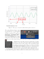
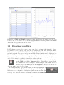
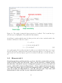
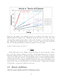
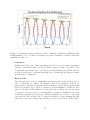
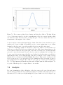
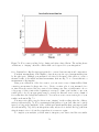
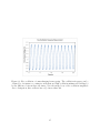
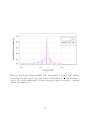
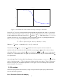
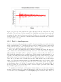
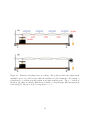
Figure 8.3: Damped harmonic motion. The characteristic damping time in this case is about
9.5 seconds, which corresponds to a Q of about 20.
seconds and up to 1 minute and then copy your voltage vs. time data into Excel for your
records. Sometimes the force sensors show a significant drift in their mean value over the
course of 20 seconds, so you may want to write down an estimate for this drift or to “warm
up” the sensor by letting your weight oscillate on the force sensor for a few minutes. This
effect is more important for the damped motion, so be sure to keep an eye on it and to either
quantify the drift or find a way to remove it for the next part.
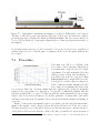
Next, you will record the same time-domain data with the damping term added. Arrange
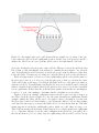
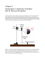
the aluminum tube to surround the oscillating weight without touching it. The magnets in
the weight will produce a damping force when the tube surrounds the moving weight. Record
the force sensor reading vs. time again and save your data. You will notice a significant decay
in the oscillation amplitude as a function of time, as shown in Fig. 8.3.
8.3
Analysis
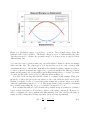
Plot your displacement vs. weight data and fit a line to determine the spring constant. Use
a regression analysis to get an error bar on the slope, as usual. Combine this with your
measured mass of the weight with embedded magnets to come up with a prediction for the
free oscillation frequency fo using Eq. 8.1.
Next, you will measure the frequency of free oscillations directly from your time-domain
voltage vs. time data. Plot your data and use the positions of the extrema to determine the
oscillation frequency. You can do this by, for instance, zooming in on the first maximum
66