1
Uppaal Tiga User-manual
Gerd Behrmann1 , Agn`es Cougnard1 , Alexandre David1 , Emmanuel Fleury2 ,
Kim G. Larsen1 , Didier Lime3
1
CISS, Aalborg University, Aalborg, Denmark
{behrmann,acougnar,adavid,kgl}@cs.aau.dk
2
3
LaBRI, Bordeaux-1 University, CNRS (UMR 5800), Talence, France
[email protected]
´
IRCCyN, Ecole
Centrale de Nantes, CNRS (UMR 6597), Nantes, France
[email protected]
Abstract. Uppaal Tiga is a tool to perform automatic synthesis of
controllers for timed systems. This document is the user-manual of Uppaal Tiga but should be read jointly with the Uppaal tutorial [BDL04].
1
Introduction
Tiga is part of the Uppaal toolbox for verification of real-time systems which
provides several verification tools such as: Uppaal1 [BDL04] (Real-time Verification), Cora2 [BLR05] (Real-time Scheduling), TROn3 [LMN05] (Online
Real-time Testing), Tiga4 (Timed Games), CoVer5 (Test-case Generation) and
Times6 (Schedulability Analysis).
Tiga is implementing a real on-the-fly algorithm to synthesize winning strategies [LS98,CDF+ 05]. Since our first prototype in 2005 [CDF+ 05], Tiga has improved of several orders of magnitude and is now ready to deal with industrial
case studies. Moreover, all the features of Uppaal are now supported allowing
the user to have a rich specification language (integer variables, templates, array
of variables, . . . ) to create its models.
Our input models are specified through a network of Timed Game Automata [MPS95] (TGA) where edges are marked either controllable or uncontrollable (see Fig.1). This defines a two players game with on one side the controller
(mastering the controllable edges) and on the other side the environment (mastering the uncontrollable edges). Winning conditions of the game are specified
through TCTL formulae. By now, Tiga supports both reachability and safety
games. Given a model and winning conditions, Tiga is able to say if ’yes’ or
1
2
3
4
5
6
http://www.uppaal.com
http://www.cs.auc.dk/~behrmann/cora/
http://www.cs.aau.dk/~marius/tron/
http://www.cs.aau.dk/~adavid/tiga/
http://user.it.uu.se/~hessel/CoVer/
http://www.timestool.com/
’no’ there is a strategy for the controller to win the game and can provide the
strategy as an output if asked (option -t0).
L0
x < 1;
x := 0
x>1
L4
x≤1
L1
x≤1
Goal
x<1
x≤1
L2
L3
Fig. 1. An example of Timed Game Automaton.
The graphical user-interface has been augmented to deal with games models.
Among other things, the simulator allows the user to play against the strategies
synthesized by Tiga in order to give the understanding of what the strategy is.
This user-manual is covering the specificities of Tiga compared to the basic Uppaal tool. It is, then, strongly advised to start with the Uppaal tutorial [BDL04] to know about the basics of Uppaal before reading this document.
We first define our game model (section 2) and how to specify games (section 3), then we explain what are strategies, how to query for a controller and
how to play with it and how to interpret results (section 4).
2
Timed Game Model
Our formalism is based on networks of Timed Game Automata (TGA) as described in [CDF+ 05,MPS95]. Given a network of timed game automata we define
two types of games, namely reachability and safety games. This section briefly recalls the definition of networks of timed game automata, reachability and safety
games and the notion of strategy over a game. We suppose here that the reader
is already familiar with timed automata as defined in [BDL04].
2.1
Timed Game Automata
Let C be a finite set of real-valued variables called clocks. We note B(C) the
set of rectangular constraints ϕ generated by the grammar: ϕ ::= x ∼ k | ϕ ∧ ϕ
where k ∈ Z, x ∈ C and ∼∈ {<, ≤, =, >, ≥}.
A Timed Game Automaton (TGA) is a timed automaton as defined in [BDL04]
such that A = (L, l0 , C, Act, E, I) with its set of actions Act = Actc ∪ Actu partitioned into controllable (Actc ) and uncontrollable (Actu ) actions. L is the set
2
of locations, l0 ∈ L the initial location, E ∈ L × Act × B(C) × 2C × L the transitions of the automaton and I : L → B(C) the location invariants. Fig. 1. gives
an example of a timed game automaton.
The semantics of a timed automaton A = (L, l0 , C, Act, E, I) is defined as
a labelled transition system hS, s0 , →i where S ⊆ L × RC is the set of states,
s0 = (l0 , 0) is the initial state (where 0 is a clock valuation in which every clock
value is 0) and →⊆ S × {R≥0 ∪ Act} × S is the transition relation such that:
d
– (l, u) −
→ (l, u + d) if ∀d′ : 0 ≤ d′ ≤ d ⇒ u + d′ |= I(l)
a
– (l, u) −
→ (l′ , u′ ) if ∃e = (l, a, g, r, l′ ) ∈ E s.t. u |= g and u′ = [r → 0]u and
′
u |= I(l′ ).
Timed game automata can be composed into networks over a common set of
actions and clocks consisting of n timed game automata Ai = (Li , l0i , C, Act, Ei , Ii )
where the set of actions over the network is given by Act = Act × Act and is such
that Act = Actc ∪ Actu where Actc = Actc × {Actc ∪ {τ }} and Actu = Act \ Actc .
Note that this way of defining controllable and uncontrollable actions on the
network gives precedence to the environment over the controller.
We also note a location of the system as a vector l = (l1 , . . . , ln ). We extend
the invariant functions such that I(l) = ∧i≤n Ii (li ). And we write l[li′ /li ] to denote
the vector where the ith element li of l is replaced by li′ .
Semantics of a network of n timed game automata Ai = (Li , l0i , C, Act, Ei , Ii )
is defined as a transition system hS, s0 , →i where S ⊆ (L1 × · · · × Ln ) × RC is
the set of states, s0 = (l0 , 0) where l0 = (l01 , . . . , l0n ), is the initial state and
→⊆ S × {R≥0 ∪ Act} × S is the transition relation such that:
d
→ (l, u + d) if ∀d′ : 0 ≤ d′ ≤ d ⇒ u + d′ |= I(l);
– (l, u) −
(a,τ )
′
a,g,r
– (l, u) −−−→ (l , u′ ) if l −−−→ l′ s.t. u |= g and u′ = [r → 0]u and u′ |= I(l);
(ai ,aj )
′
ai !,gi ,ri
aj ?,gj ,rj
– (l, u) −−−−→ (l [li /li′ , lj /lj′ ], u′ ) if li −−−−−→ li′ and lj −−−−−−→ lj′ s.t. u |= gi ∧ gj
and u′ = [ri ∪ rj → 0]u and u′ |= I(l′ ).
2.2
The Modelling Language
Defining a timed game automata is achieved through a superset of the Uppaal
modelling language. The only addition to the original language are the possibility
to define “uncontrollable” transitions. Either through the graphical user interface
(see Fig. 2, on the left) using the edge interface, or through the ta language
using the “-u->” keyword (see Fig. 2, on the right). Note that transitions are
assumed to be “controllable” by default and that priorities on transitions are
simply ignored when synthesizing strategies.
3
Specifying Games
A game is given by a network of timed game automata (A = (Ai )i>0 ) specifying
the rules of the game and a formula (ϕ) specifying winning conditions defining
the set of states that should be reached/avoided in order to win/lose the game.
3
process Main() {
clock x;
state L0 {x<=2}, L1, L2, L3, L4, goal;
init L0;
trans
L0 -> L1 {guard x<=1;},
L0 -u-> L2 {guard x<1;assign x=0;},
L0 -u-> L4 {guard x>1;},
L1 -> goal {guard x>=2;},
L1 -u-> L2 {guard x<1;},
L2 -> L3 { },
L3 -> L1 {guard x<=1;};
}
system Main;
Fig. 2. Tiga GUI and XTGA syntax examples
3.1
Winning Games
Winning a game can only be achieved if the last transition leading to the goal
state is controllable. For example, the automaton on Fig. 3.(a) is winning, on
the contrary the automaton on the Fig. 3.(b) is losing. Intuitively this is because
the opponent can decide to stay in the initial state forever without taking the
transition leading to the goal state and let the controller with no other choice
but its own.
Init
Init
Win!
Goal
Lose!
Goal
(a)
(b)
Fig. 3. Basic Examples of Winning (a) and Losing (b) Timed Game Automata.
The use of invariants might force the opponent to act, this can be simulated
through an implicit controllable edge added when the upper limit of the invariant
is reached. We will call this implicit extra transition a forced transition.
For example, the automaton on Fig. 4.(a) shows the original model, the
automaton on Fig. 4.(b) makes the forced transition explicit making it clear why
the model is winning7 . Finally, the automaton on Fig. 4.(c) cannot be added a
forced transition because there is already a possible controllable behavior when
the automaton hit the invariant therefore this model is declared as losing.
7
Note that forced transitions are always controllable.
4
Init
[x ≤ 5]
Win!
Goal
[x ≤ 5]
⇔
Init
x == 5
(a)
[x ≤ 5]
Win!
Init
Lose!
Goal
Goal
(c)
(b)
Fig. 4. Basic examples of forced transition: winning model (a), equivalent model with
the implicit transition made explicit (b) and a losing model (c).
Finally, when dealing with synchronization and invariants some apparently
strange behaviors might occurs. Indeed forced transitions might appear in components and be synchronized with others. The rule being to locally add forced
transitions to each component and then to compose them all together. On
Fig. 5.(a) we can see the original model of two synchronized automata, on
Fig. 5.(b) the forced transition made explicit and finally on Fig. 5.(c) the full
composition of the model (with the explicit forced transition).
[x ≤ 5]
a == 0
Goal
[x ≤ 5]
[x ≤ 5]
Inita
k
Initb
⇔
a=1
a == 0
∧
x == 5
Inita
a == 0
Goal
Win!
(a)
k
Initb
a=1
⇔
a == 0
∧
x == 5
Win!
(b)
Inita,b
a=1
a == 0
Goal Win!
(c)
Fig. 5. Example of synchronisation with forced transitions: original model (a), forced
transition made explicit (b), complete product with forced transition made explicit.
3.2
Winning/Losing Conditions
Specifying the game still requires to define what are the winning conditions. This
is done through a slightly modified version of the Uppaal query language. Given
a timed game automaton A, a set of goal states (win) and/or a set of bad states
(lose), both defined by classical Uppaal state formulae, four types of winning
conditions can be issued. For all of them, the game is to find a controllable
strategy f such that A supervised by f ensures that the controller:
– Pure Reachability:
“must reach win”
control: A<> win
– Strict Reachability with Avoidance (Until):
“must reach win and must avoid lose”
control: A[ not(lose) U win ]
5
– Weak Reachability with Avoidance (WeakUntil):
“should reach win and must avoid lose”
control: A[ not(lose) W win ]
– Pure Safety:
“must avoid lose”
control: A[] not(lose)
Note : Formulae not prefixed by “control:” are solved as in usual Uppaal. Also,
the operators A[p U q] and A[p W q] are Tiga specific and are not supported
by Uppaal.
Examples:
–
–
–
–
–
3.3
control:
control:
control:
control:
control:
A<> Main.goal
A[] not Main.L4
A[ not Main.L4 W Main.goal ]
A[ Main.x<2 U Main.goal ]
A[ not(Main.goal and Main.x>2) U (Main.goal) ]
Partially Cooperative Games
Partially cooperative games are defined by the fact that there are no winning
strategy but reaching a maximal partition with winning strategy can be done
with some help from your opponent. Once inside the maximal partition, you can
enforce some condition whatever decide the oponnent. On Fig. 6, the maximal
partition is the gray part and in order to reach it the controller has to rely on
the environment to do some moves in his favor.
Init
E<>
control:ϕ
Fig. 6. Representation of E<>control:ϕ.
The syntax of this formula is given by:
– Partial Cooperation:
“must satisfy ϕ with the least help from the environment”
E<> control: ϕ
6
4
Strategy Synthesis
A (controllable) strategy is a function f : L × RC
≥0 → Actc ∪ {λ} that constantly
gives information as to what the controller should do during the course of the
game. In a given situation, the strategy could suggest the controller to either
“do a particular controllable action” or “do nothing at this point in time (λ)”.
A strategy is said to be a winning strategy if the controller supervised by the
strategy always win the game whatever actions are chosen by the environment.
4.1
Existence of a Strategy
By default, Tiga first check whether there is or not a winning strategy for the
timed game given a winning condition. On the example given Fig. 7, a winning
strategy can be extracted for all the specified winning conditions except for the
fifth one. Note that it is always better to start asking for existence because the
process of strategy extraction is quite demanding and it would be useless to run
such computation when the strategy can not be found.
#shell> verifytga concur05-1.{xml,q}
Options for the verification:
Generating no trace
Search order is breadth first
Using conservative space optimisation
Seed is 1156870160
State space representation
uses minimal constraint systems
Verifying property 1 at line 5
-- Property is satisfied.
Verifying property 2 at line 11
-- Property is satisfied.
Verifying property 3 at line 17
-- Property is satisfied.
Verifying property 4 at line 23
-- Property is satisfied.
Verifying property 5 at line 29
-- Property is NOT satisfied.
Verifying property 6 at line 35
-- Property is satisfied.
Fig. 7. TGA synthesis example and the Tiga GUI
4.2
Strategy Extraction (Option -t0)
The command line tool verifytga in the Tiga package can output a strategy
for each given winning condition when used with the “-t0” option. If no such
7
strategy exists, the dual strategy can then be computed by Tiga 8 . The extraction of a strategy can be triggered through a set of options specific to the Tiga
engine:
-t <0|1|2>
Generate diagnostic information
0: Some trace and output some
-c <0|1>
Print compact strategy
0: Print one strategy for each
1: Dump BCDD strategy for each
on stderr.
strategy
discrete state
transition
An example of such output is given for the concur05-1.xml example on
Fig. 8 with the options “-t0 -c0”.
State: ( Main.L0 )
While you are in (Main.x<1), wait.
When you are in (Main.x==1),
take transition Main.L0->Main.L1 { x <= 1, tau, 1 }
State: ( Main.L1 )
While you are in (1<=Main.x && Main.x<2) || (Main.x<1), wait.
When you are in (2<=Main.x),
take transition Main.L1->Main.goal { x >= 2, tau, 1 }
State: ( Main.L2 )
When you are in (Main.x<=1),
take transition Main.L2->Main.L3 { 1, tau, 1 }
State: ( Main.L3 )
When you are in (Main.x==1),
take transition Main.L3->Main.L1 { x <= 1, tau, 1 }
While you are in (Main.x<1), wait.
Fig. 8. Strategy Synthesized for concur05-1.xml for “control: A<> Main.goal”.
4.3
Time Optimal Strategies
One may want not ’any strategy’ but the most time efficient Tiga can find.
– Time Optimality:
“must reach win within less than u-g time units and must avoid lose”
control t*(u,g): A[ not(lose) U win ]
8
We plan to add an option “-d” (dual) to compute automatically the dual strategy.
8
Fig. 9 shows an example of use of control t*(u,g), where only the winning
paths that can reach the winning location within u−g are accepted thus allowing
to forge a winning strategy based on this new winning conditions. Please note
that the strategy that you play in the simulator has all its states constrained by
u − g.
Win
Win
Init
u
Win
g
Fig. 9. Using the control t*(u,g):A[p U q] expression.
Provided that Tiga stop on some winning-strategy for our property, we can
give an always terminating approximation algorithm to refine the first winning
strategy. Indeed, start with u being the minimum time needed to reach the
winning state on the strategy outputted by Tiga and with g = 0. Then, increase
g until you reach a g ′ such that g ′ gives a winning strategy and g ′ + 1 does not
or do not terminate. This will provide you with the best strategy Tiga can give
you (if not the optimal one).
Moreover, the u and g expression can be made more complex than constants.
Indeed, it accepts the full C-like Uppaal syntax with the limitations that u is
evaluated once at the beginning so it should not depend on the current state or
contain clock constraints, and g is evaluated on the current state but must be
side-effect free, which is no clock constraints here as well. An adequate usage
of the function time2goal() (quantifying the time left before reaching any goal
state) can help a lot when searching for an optimal strategy. The formula would
be: control t*(u,time2goal()). Where u being the result of a non constrained
search for strategy performed before. The time2goal() part will help here to
prune a lot of non-optimal behavior and will help to reach time optimality.
4.4
Concrete Game Simulator
A new feature since Uppaal Tiga 0.11 is the concrete simulator. Up to 0.10,
the simulator was a symbolic one, you can now simulate your system based
on concrete trace that you choose or that you can randomely fire throught the
”Random” button.
Concrete simulator help you to select a transition to fire and then at what
time it will be fired. The ”transition selection” area is a clickable area where
vertical axis displays the active transtion at this location and horizontal axis
displays the time at which the transition will be fired. By clicking in a valid zone
9
Fig. 10. Tiga concrete simulator with highlights on Transition selection, Time selection, Run History and Heat bar.
within this area make you select a precise transition and time for this transition.
The time selected is displayed in the ”Time Selection” area.
Two new graphical elements are also appearing in the new concrete simulator.
One is the ”Run History” area which allow a quick navigation in the history of
the run that you explore. The gray part of an history item visualize the time
elapsed within this state. Finally, the other element is the ”Heat Bar ” allowing to
visualize the activity (rate of actions taken over the time). More blue it is, colder
you are by waiting a lot in states. More red it is, hotter you are by performing
a lot of actions in short time.
The concrete simulator is extremely useful at debug time to understand why
a winning condition cannot be met. Playing against the dual strategy allow to
test intuitive strategies or to discover tactics used by the environment to defeat
the controller.
5
Conclusion & Further Works
Tiga is already fully functional and provide a full support of all the Uppaal
features plus an extended query language to specify winning conditions. Tiga is
able to detect strategy existence and to synthesize it at will. An interactive simulator also allow the user to try out the strategy of the controller or the strategy of
10
the opponent. Moreover, several industrial case studies [DJLR07,CDL07,LC04]
have been conducted with success.
In [DJLR07], the synthesis capability of the tool has been combined with
Simulink and Real-Time Workshop to provide a complete tool chain for synthesis,
simulation, and automatic generation of production code. This work has been
performed in collaboration with the company Skov A/S specializing in climate
control systems used for modern pig and poultry stables.
Tiga has also been use to check for simulation between timed automata
and timed game automata [CDL07]. Given two timed automata, the tool can
check if one simulates the other and similarly for timed game automata with
applications for controller synthesis with partial observability. This technique has
been applied to the compositional verification of the ZeroConf protocol [GVZ06].
Our tool is being used in the AMAES project9 , a French national project on
’Advanced Methods for Autonomous Embedded Systems’. Tiga has been applied
for controlling the autonomous robot Dala [LC04] in charge of taking pictures
and transmitting them back to Earth during limited transmission windows. It is
desirable in such control problems to optimize the moves to save power.
In the near future we plan to improve efficiency of the state-space exploration
again and to look at partial observability and focus on more and more real-life
problems.
References
[BDL04] G. Behrmann, A. David, and K. G. Larsen. A Tutorial on Uppaal. In
Proc. of 4th Int. School on Formal Methods for the Design of Computer,
Communication, & Software Systems (SFM-RT04), number 3185 in LNCS,
pages 200–236. Springer, 2004.
[BLR05] G. Behrmann, K. G. Larsen, and J. I. Rasmussen. Priced Timed Automata:
Decidability Results, Algorithms and Applications. In Proc. of 3rd International Symposium Formal Methods for Components and Objects (FMCO
2004), volume 3657 of LNCS, pages 162–182, Leiden, The Netherlands,
November 2005. Springer.
[CDF+ 05] F. Cassez, A. David, E. Fleury, K. G. Larsen, and D. Lime. Efficient Onthe-fly Algorithms for the Analysis of Timed Games. In Proc. of 16th Int.
Conf. on Concurrency Theory (CONCUR’05), volume 3653 of LNCS, pages
66–80. Springer, 2005.
[CDL07] T. Chatain, A. David, and K. G. Larsen. Playing Games with Games. In
Submitted to CAV’07, 2007.
[DJLR07] A. David, J. J. Jessen, K. G. Larsen, and J. I. Rasmussen. Guided Controller Synthesis for Climate Controller Using uppaal-tiga. In Submitted
to CAV’07, 2007.
[GVZ06] B. Gebremichael, F. W. Vaandrager, and M. Zhang. Analysis of the zeroconf
protocol using uppaal. In Proceedings 6th Annual ACM & IEEE Conference
on Embedded Software (EMSOFT 2006), pages 242–251, 2006.
9
http://www-verimag.imag.fr/∼krichen/AMAES/
11
[LC04]
S. Lemai-Chenevier. IxTeT-eXeC: Planification, r´eparation de plan et
contrˆ
ole d’ex´ecution avec gestion du temps et des ressources. PhD thesis,
Institut National Polytechnique de Toulouse, 2004.
[LMN05] K. G. Larsen, M. Mikucionis, and B. Nielsen. Online Testing of RealTime Systems Using UPPAAL: Status and Future Work. In In Proc.
of Perspectives of Model-Based Testing, number 04371 in Dagstuhl Seminar Proceedings, Dagstuhl, Germany, 2005. Internationales Begegnungs und
Forschungszentrum f¨
ur Informatik (IBFI).
[LS98]
X. Liu and S. Smolka. Simple Linear-Time Algorithm for Minimal Fixed
Points. In Proc. 26th Conf. on Automata, Languages and Programming
(ICALP’98), volume 1443 of LNCS, pages 53–66. Springer, 1998.
[MPS95] O. Maler, A. Pnueli, and J. Sifakis. On the Synthesis of Discrete Controllers
for Timed Systems. In Proc. 12th Symp. on Theoretical Aspects of Computer
Science (STACS’95), volume 900, pages 229–242. Springer, 1995.
12