Download Matpower 5.1 User`s Manual - Power Systems Engineering

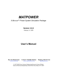
Matpower 5.1
User’s Manual
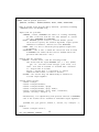
Ray D. Zimmerman
Carlos E. Murillo-Sánchez
March 20, 2015
© 2010, 2011, 2012, 2013, 2014, 2015 Power Systems Engineering Research Center (Pserc)
All Rights Reserved
Contents
1 Introduction
1.1 Background . . . . . . . . . . . . . . . . . . . . . . . . . . . . . . . .
1.2 License and Terms of Use . . . . . . . . . . . . . . . . . . . . . . . .
1.3 Citing Matpower . . . . . . . . . . . . . . . . . . . . . . . . . . . .
9
9
10
11
2 Getting Started
2.1 System Requirements . . . .
2.2 Installation . . . . . . . . .
2.3 Running a Simulation . . . .
2.3.1 Preparing Case Input
2.3.2 Solving the Case . .
2.3.3 Accessing the Results
2.3.4 Setting Options . . .
2.4 Documentation . . . . . . .
. . . .
. . . .
. . . .
Data .
. . . .
. . . .
. . . .
. . . .
.
.
.
.
.
.
.
.
.
.
.
.
.
.
.
.
.
.
.
.
.
.
.
.
.
.
.
.
.
.
.
.
.
.
.
.
.
.
.
.
.
.
.
.
.
.
.
.
.
.
.
.
.
.
.
.
.
.
.
.
.
.
.
.
.
.
.
.
.
.
.
.
.
.
.
.
.
.
.
.
.
.
.
.
.
.
.
.
.
.
.
.
.
.
.
.
.
.
.
.
.
.
.
.
.
.
.
.
.
.
.
.
.
.
.
.
.
.
.
.
.
.
.
.
.
.
.
.
.
.
.
.
.
.
.
.
.
.
.
.
.
.
.
.
.
.
.
.
.
.
.
.
12
12
12
15
16
16
17
18
18
3 Modeling
3.1 Data Formats . . .
3.2 Branches . . . . . .
3.3 Generators . . . . .
3.4 Loads . . . . . . .
3.5 Shunt Elements . .
3.6 Network Equations
3.7 DC Modeling . . .
.
.
.
.
.
.
.
.
.
.
.
.
.
.
.
.
.
.
.
.
.
.
.
.
.
.
.
.
.
.
.
.
.
.
.
.
.
.
.
.
.
.
.
.
.
.
.
.
.
.
.
.
.
.
.
.
.
.
.
.
.
.
.
.
.
.
.
.
.
.
.
.
.
.
.
.
.
.
.
.
.
.
.
.
.
.
.
.
.
.
.
.
.
.
.
.
.
.
.
.
.
.
.
.
.
.
.
.
.
.
.
.
.
.
.
.
.
.
.
.
.
.
.
.
.
.
.
.
.
.
.
.
.
.
.
.
.
.
.
.
21
21
21
23
23
23
24
24
.
.
.
.
28
28
30
30
32
.
.
.
.
.
35
36
36
37
37
38
4 Power Flow
4.1 AC Power Flow . .
4.2 DC Power Flow . .
4.3 runpf . . . . . . .
4.4 Linear Shift Factors
.
.
.
.
.
.
.
.
.
.
.
.
.
.
.
.
.
.
.
.
.
.
.
.
.
.
.
.
.
.
.
.
.
5 Continuation Power Flow
5.1 Parameterization . . . .
5.2 Predictor . . . . . . . . .
5.3 Corrector . . . . . . . .
5.4 Step length control . . .
5.5 runcpf . . . . . . . . . .
.
.
.
.
.
.
.
.
.
.
.
.
.
.
.
.
.
.
.
.
.
.
.
.
.
.
.
.
.
.
.
.
.
.
.
.
.
.
.
.
.
.
.
.
.
.
.
.
.
.
.
.
.
.
.
.
.
.
.
.
.
.
.
.
.
.
.
.
.
.
.
.
.
2
.
.
.
.
.
.
.
.
.
.
.
.
.
.
.
.
.
.
.
.
.
.
.
.
.
.
.
.
.
.
.
.
.
.
.
.
.
.
.
.
.
.
.
.
.
.
.
.
.
.
.
.
.
.
.
.
.
.
.
.
.
.
.
.
.
.
.
.
.
.
.
.
.
.
.
.
.
.
.
.
.
.
.
.
.
.
.
.
.
.
.
.
.
.
.
.
.
.
.
.
.
.
.
.
.
.
.
.
.
.
.
.
.
.
.
.
.
.
.
.
.
.
.
.
.
.
.
.
.
.
.
.
.
.
.
.
.
.
.
.
.
.
.
.
.
.
.
.
.
.
.
.
.
.
.
.
.
.
.
.
.
.
.
.
.
.
.
.
.
.
.
.
.
.
.
.
.
.
6 Optimal Power Flow
6.1 Standard AC OPF . . . . . . . . . . .
6.2 Standard DC OPF . . . . . . . . . . .
6.3 Extended OPF Formulation . . . . . .
6.3.1 User-defined Costs . . . . . . .
6.3.2 User-defined Constraints . . . .
6.3.3 User-defined Variables . . . . .
6.4 Standard Extensions . . . . . . . . . .
6.4.1 Piecewise Linear Costs . . . . .
6.4.2 Dispatchable Loads . . . . . . .
6.4.3 Generator Capability Curves . .
6.4.4 Branch Angle Difference Limits
6.5 Solvers . . . . . . . . . . . . . . . . . .
6.6 runopf . . . . . . . . . . . . . . . . . .
.
.
.
.
.
.
.
.
.
.
.
.
.
.
.
.
.
.
.
.
.
.
.
.
.
.
.
.
.
.
.
.
.
.
.
.
.
.
.
.
.
.
.
.
.
.
.
.
.
.
.
.
.
.
.
.
.
.
.
.
.
.
.
.
.
.
.
.
.
.
.
.
.
.
.
.
.
.
.
.
.
.
.
.
.
.
.
.
.
.
.
.
.
.
.
.
.
.
.
.
.
.
.
.
.
.
.
.
.
.
.
.
.
.
.
.
.
.
.
.
.
.
.
.
.
.
.
.
.
.
.
.
.
.
.
.
.
.
.
.
.
.
.
.
.
.
.
.
.
.
.
.
.
.
.
.
.
.
.
.
.
.
.
.
.
.
.
.
.
.
.
.
.
.
.
.
.
.
.
.
.
.
.
.
.
.
.
.
.
.
.
.
.
.
.
.
.
.
.
.
.
.
.
.
.
.
.
.
44
44
45
46
46
47
49
49
49
50
52
52
53
54
7 Extending the OPF
7.1 Direct Specification . . . . . . . . . . . . .
7.2 Callback Functions . . . . . . . . . . . . .
7.2.1 ext2int Callback . . . . . . . . . .
7.2.2 formulation Callback . . . . . . .
7.2.3 int2ext Callback . . . . . . . . . .
7.2.4 printpf Callback . . . . . . . . . .
7.2.5 savecase Callback . . . . . . . . .
7.3 Registering the Callbacks . . . . . . . . . .
7.4 Summary . . . . . . . . . . . . . . . . . .
7.5 Example Extensions . . . . . . . . . . . .
7.5.1 Fixed Zonal Reserves . . . . . . . .
7.5.2 Interface Flow Limits . . . . . . . .
7.5.3 DC Transmission Lines . . . . . . .
7.5.4 DC OPF Branch Flow Soft Limits .
.
.
.
.
.
.
.
.
.
.
.
.
.
.
.
.
.
.
.
.
.
.
.
.
.
.
.
.
.
.
.
.
.
.
.
.
.
.
.
.
.
.
.
.
.
.
.
.
.
.
.
.
.
.
.
.
.
.
.
.
.
.
.
.
.
.
.
.
.
.
.
.
.
.
.
.
.
.
.
.
.
.
.
.
.
.
.
.
.
.
.
.
.
.
.
.
.
.
.
.
.
.
.
.
.
.
.
.
.
.
.
.
.
.
.
.
.
.
.
.
.
.
.
.
.
.
.
.
.
.
.
.
.
.
.
.
.
.
.
.
.
.
.
.
.
.
.
.
.
.
.
.
.
.
.
.
.
.
.
.
.
.
.
.
.
.
.
.
.
.
.
.
.
.
.
.
.
.
.
.
.
.
.
.
.
.
.
.
.
.
.
.
.
.
.
.
.
.
.
.
.
.
.
.
.
.
.
.
.
.
59
59
60
61
63
65
67
70
72
74
74
74
75
76
79
.
.
.
.
.
.
.
.
.
.
.
.
.
8 Unit De-commitment Algorithm
82
9 Miscellaneous Matpower Functions
9.1 Input/Output Functions . . . . . .
9.1.1 loadcase . . . . . . . . . .
9.1.2 savecase . . . . . . . . . .
9.1.3 cdf2mpc . . . . . . . . . . .
9.1.4 psse2mpc . . . . . . . . . .
84
84
84
84
85
85
3
.
.
.
.
.
.
.
.
.
.
.
.
.
.
.
.
.
.
.
.
.
.
.
.
.
.
.
.
.
.
.
.
.
.
.
.
.
.
.
.
.
.
.
.
.
.
.
.
.
.
.
.
.
.
.
.
.
.
.
.
.
.
.
.
.
.
.
.
.
.
.
.
.
.
.
.
.
.
.
.
.
.
.
.
.
.
.
.
.
.
.
.
.
.
.
9.2
9.3
9.4
9.5
9.6
System Information . . . . . . . . . . . . . . . . . . .
9.2.1 case info . . . . . . . . . . . . . . . . . . . .
9.2.2 compare case . . . . . . . . . . . . . . . . . .
9.2.3 find islands . . . . . . . . . . . . . . . . . .
9.2.4 get losses . . . . . . . . . . . . . . . . . . .
9.2.5 margcost . . . . . . . . . . . . . . . . . . . .
9.2.6 isload . . . . . . . . . . . . . . . . . . . . . .
9.2.7 printpf . . . . . . . . . . . . . . . . . . . . .
9.2.8 total load . . . . . . . . . . . . . . . . . . .
9.2.9 totcost . . . . . . . . . . . . . . . . . . . . .
Modifying a Case . . . . . . . . . . . . . . . . . . . .
9.3.1 extract islands . . . . . . . . . . . . . . . .
9.3.2 load2disp . . . . . . . . . . . . . . . . . . . .
9.3.3 modcost . . . . . . . . . . . . . . . . . . . . .
9.3.4 scale load . . . . . . . . . . . . . . . . . . .
Conversion between External and Internal Numbering
9.4.1 ext2int, int2ext . . . . . . . . . . . . . . . .
9.4.2 e2i data, i2e data . . . . . . . . . . . . . . .
9.4.3 e2i field, i2e field . . . . . . . . . . . . .
Forming Standard Power Systems Matrices . . . . . .
9.5.1 makeB . . . . . . . . . . . . . . . . . . . . . .
9.5.2 makeBdc . . . . . . . . . . . . . . . . . . . . .
9.5.3 makeJac . . . . . . . . . . . . . . . . . . . . .
9.5.4 makeYbus . . . . . . . . . . . . . . . . . . . .
Miscellaneous . . . . . . . . . . . . . . . . . . . . . .
9.6.1 define constants . . . . . . . . . . . . . . .
9.6.2 have fcn . . . . . . . . . . . . . . . . . . . .
9.6.3 mpver . . . . . . . . . . . . . . . . . . . . . .
9.6.4 nested struct copy . . . . . . . . . . . . . .
.
.
.
.
.
.
.
.
.
.
.
.
.
.
.
.
.
.
.
.
.
.
.
.
.
.
.
.
.
.
.
.
.
.
.
.
.
.
.
.
.
.
.
.
.
.
.
.
.
.
.
.
.
.
.
.
.
.
.
.
.
.
.
.
.
.
.
.
.
.
.
.
.
.
.
.
.
.
.
.
.
.
.
.
.
.
.
.
.
.
.
.
.
.
.
.
.
.
.
.
.
.
.
.
.
.
.
.
.
.
.
.
.
.
.
.
.
.
.
.
.
.
.
.
.
.
.
.
.
.
.
.
.
.
.
.
.
.
.
.
.
.
.
.
.
.
.
.
.
.
.
.
.
.
.
.
.
.
.
.
.
.
.
.
.
.
.
.
.
.
.
.
.
.
.
.
.
.
.
.
.
.
.
.
.
.
.
.
.
.
.
.
.
.
.
.
.
.
.
.
.
.
.
.
.
.
.
.
.
.
.
.
.
.
.
.
.
.
.
.
.
.
.
.
.
.
.
.
.
.
.
.
.
.
.
.
.
.
.
.
.
.
.
.
.
.
.
.
.
.
.
.
.
.
.
.
.
.
.
.
.
10 Acknowledgments
85
85
86
86
86
87
87
87
88
88
88
88
89
89
89
90
90
90
91
91
91
92
92
92
92
92
93
93
94
95
Appendix A MIPS – Matlab Interior Point Solver
A.1 Example 1 . . . . . . . . . . . . . . . . . . . . . .
A.2 Example 2 . . . . . . . . . . . . . . . . . . . . . .
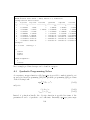
A.3 Quadratic Programming Solver . . . . . . . . . .
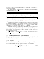
A.4 Primal-Dual Interior Point Algorithm . . . . . . .
A.4.1 Notation . . . . . . . . . . . . . . . . . . .
4
.
.
.
.
.
.
.
.
.
.
.
.
.
.
.
.
.
.
.
.
.
.
.
.
.
.
.
.
.
.
.
.
.
.
.
.
.
.
.
.
.
.
.
.
.
.
.
.
.
.
.
.
.
.
.
96
98
100
102
103
103
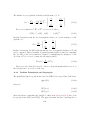
A.4.2 Problem Formulation and Lagrangian . . . . . . . . . . . . . . 104
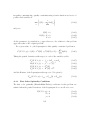
A.4.3 First Order Optimality Conditions . . . . . . . . . . . . . . . 105
A.4.4 Newton Step . . . . . . . . . . . . . . . . . . . . . . . . . . . 106
Appendix B Data File Format
109
Appendix C Matpower Options
115
C.1 Mapping of Old-Style Options to New-Style Options . . . . . . . . . . 130
Appendix D Matpower Files and
D.1 Documentation Files . . . . .
D.2 Matpower Functions . . . .
D.3 Example Matpower Cases .
D.4 Automated Test Suite . . . .
Functions
. . . . . . .
. . . . . . .
. . . . . . .
. . . . . . .
.
.
.
.
.
.
.
.
.
.
.
.
.
.
.
.
.
.
.
.
.
.
.
.
.
.
.
.
.
.
.
.
.
.
.
.
.
.
.
.
.
.
.
.
.
.
.
.
.
.
.
.
.
.
.
.
.
.
.
.
Appendix E Extras Directory
134
134
134
143
144
148
Appendix F “Smart Market” Code
149
F.1 Handling Supply Shortfall . . . . . . . . . . . . . . . . . . . . . . . . 151
F.2 Example . . . . . . . . . . . . . . . . . . . . . . . . . . . . . . . . . . 151
F.3 Smartmarket Files and Functions . . . . . . . . . . . . . . . . . . . . 155
Appendix G Optional Packages
G.1 BPMPD MEX – MEX interface for BPMPD . . . . . . . . . . . . . .
G.2 CLP – COIN-OR Linear Programming . . . . . . . . . . . . . . . . .
G.3 CPLEX – High-performance LP and QP Solvers . . . . . . . . . . . .
G.4 GLPK – GNU Linear Programming Kit . . . . . . . . . . . . . . . .
G.5 Gurobi – High-performance LP and QP Solvers . . . . . . . . . . . .
G.6 Ipopt – Interior Point Optimizer . . . . . . . . . . . . . . . . . . . .
G.7 KNITRO – Non-Linear Programming Solver . . . . . . . . . . . . . .
G.8 MINOPF – AC OPF Solver Based on MINOS . . . . . . . . . . . . .
G.9 MOSEK – High-performance LP and QP Solvers . . . . . . . . . . .
G.10 PARDISO – Parallel Sparse Direct and Multi-Recursive Iterative Linear Solvers . . . . . . . . . . . . . . . . . . . . . . . . . . . . . . . . .
G.11 SDP PF – Applications of a Semidefinite Programming Relaxation of
the Power Flow Equations . . . . . . . . . . . . . . . . . . . . . . . .
G.12 TSPOPF – Three AC OPF Solvers by H. Wang . . . . . . . . . . . .
157
157
157
158
159
159
160
161
162
162
References
165
5
163
163
163
List of Figures
3-1
5-1
6-1
6-2
6-3
6-4
6-5
6-6
7-1
7-2
7-3
7-4
Branch Model . . . . . . . . . . . . . . . . . . . . . . .
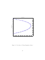
Nose Curve of Voltage Magnitude at Bus 9 . . . . . . .
Relationship of wi to ri for di = 1 (linear option) . . . .
Relationship of wi to ri for di = 2 (quadratic option) .
Constrained Cost Variable . . . . . . . . . . . . . . . .
Marginal Benefit or Bid Function . . . . . . . . . . . .
Total Cost Function for Negative Injection . . . . . . .
Generator P -Q Capability Curve . . . . . . . . . . . .
Adding Constraints Across Subsets of Variables . . . .
DC Line Model . . . . . . . . . . . . . . . . . . . . . .
Equivalent “Dummy” Generators . . . . . . . . . . . .
Feasible Region for Branch Flow Violation Constraints
.
.
.
.
.
.
.
.
.
.
.
.
.
.
.
.
.
.
.
.
.
.
.
.
.
.
.
.
.
.
.
.
.
.
.
.
.
.
.
.
.
.
.
.
.
.
.
.
.
.
.
.
.
.
.
.
.
.
.
.
.
.
.
.
.
.
.
.
.
.
.
.
.
.
.
.
.
.
.
.
.
.
.
.
.
.
.
.
.
.
.
.
.
.
.
.
22
42
48
48
50
51
51
53
64
77
77
79
Power Flow Results . . . . . . . . . . . . . . . . . . . . . . . .
Power Flow Options . . . . . . . . . . . . . . . . . . . . . . .
Power Flow Output Options . . . . . . . . . . . . . . . . . . .
Continuation Power Flow Results . . . . . . . . . . . . . . . .
Continuation Power Flow Options . . . . . . . . . . . . . . . .
Continuation Power Flow Callback Arguments . . . . . . . . .
Optimal Power Flow Results . . . . . . . . . . . . . . . . . . .
Optimal Power Flow Solver Options . . . . . . . . . . . . . . .
Other OPF Options . . . . . . . . . . . . . . . . . . . . . . . .
OPF Output Options . . . . . . . . . . . . . . . . . . . . . . .
Names Used by Implementation of OPF with Reserves . . . .
Results for User-Defined Variables, Constraints and Costs . . .
Callback Functions . . . . . . . . . . . . . . . . . . . . . . . .
Input Data Structures for Interface Flow Limits . . . . . . . .
Output Data Structures for Interface Flow Limits . . . . . . .
Input Data Structures for DC OPF Branch Flow Soft Limits .
Output Data Structures for DC OPF Branch Flow Soft Limits
Input Arguments for mips . . . . . . . . . . . . . . . . . . . .
Output Arguments for mips . . . . . . . . . . . . . . . . . . .
Options for mips . . . . . . . . . . . . . . . . . . . . . . . . .
Bus Data (mpc.bus) . . . . . . . . . . . . . . . . . . . . . . . .
.
.
.
.
.
.
.
.
.
.
.
.
.
.
.
.
.
.
.
.
.
.
.
.
.
.
.
.
.
.
.
.
.
.
.
.
.
.
.
.
.
.
.
.
.
.
.
.
.
.
.
.
.
.
.
.
.
.
.
.
.
.
.
. 31
. 31
. 32
. 38
. 39
. 40
. 55
. 57
. 58
. 58
. 62
. 66
. 74
. 76
. 76
. 80
. 80
. 97
. 98
. 99
. 110
List of Tables
4-1
4-2
4-3
5-1
5-2
5-3
6-1
6-2
6-3
6-4
7-1
7-2
7-3
7-4
7-5
7-6
7-7
A-1
A-2
A-3
B-1
6
B-2 Generator Data (mpc.gen) . . . . . . . .
B-3 Branch Data (mpc.branch) . . . . . . . .
B-4 Generator Cost Data (mpc.gencost) . . .
B-5 DC Line Data (mpc.dcline) . . . . . . .
C-1 Top-Level Options . . . . . . . . . . . .
C-2 Power Flow Options . . . . . . . . . . .
C-3 Continuation Power Flow Options . . . .
C-4 OPF Solver Options . . . . . . . . . . .
C-5 General OPF Options . . . . . . . . . .
C-6 Power Flow and OPF Output Options .
C-7 OPF Options for MIPS . . . . . . . . . .
C-8 OPF Options for CLP . . . . . . . . . .
C-9 OPF Options for CPLEX . . . . . . . .
C-10 OPF Options for fmincon . . . . . . . .
C-11 OPF Options for GLPK . . . . . . . . .
C-12 OPF Options for Gurobi . . . . . . . . .
C-13 OPF Options for Ipopt . . . . . . . . .
C-14 OPF Options for KNITRO . . . . . . . .
C-15 OPF Options for MINOPF . . . . . . . .
C-16 OPF Options for MOSEK . . . . . . . .
C-17 OPF Options for PDIPM . . . . . . . . .
C-18 OPF Options for TRALM . . . . . . . .
C-19 Old-Style to New-Style Option Mapping
D-1 Matpower Documentation Files . . . .
D-2 Top-Level Simulation Functions . . . . .
D-3 Input/Output Functions . . . . . . . . .
D-4 Data Conversion Functions . . . . . . . .
D-5 Power Flow Functions . . . . . . . . . .
D-6 Continuation Power Flow Functions . . .
D-7 OPF and Wrapper Functions . . . . . .
D-8 OPF Model Objects . . . . . . . . . . .
D-9 OPF Solver Functions . . . . . . . . . .
D-10 Other OPF Functions . . . . . . . . . . .
D-11 OPF User Callback Functions . . . . . .
D-12 Power Flow Derivative Functions . . . .
D-13 NLP, LP & QP Solver Functions . . . .
D-14 Matrix Building Functions . . . . . . . .
D-15 Utility Functions . . . . . . . . . . . . .
7
.
.
.
.
.
.
.
.
.
.
.
.
.
.
.
.
.
.
.
.
.
.
.
.
.
.
.
.
.
.
.
.
.
.
.
.
.
.
.
.
.
.
.
.
.
.
.
.
.
.
.
.
.
.
.
.
.
.
.
.
.
.
.
.
.
.
.
.
.
.
.
.
.
.
.
.
.
.
.
.
.
.
.
.
.
.
.
.
.
.
.
.
.
.
.
.
.
.
.
.
.
.
.
.
.
.
.
.
.
.
.
.
.
.
.
.
.
.
.
.
.
.
.
.
.
.
.
.
.
.
.
.
.
.
.
.
.
.
.
.
.
.
.
.
.
.
.
.
.
.
.
.
.
.
.
.
.
.
.
.
.
.
.
.
.
.
.
.
.
.
.
.
.
.
.
.
.
.
.
.
.
.
.
.
.
.
.
.
.
.
.
.
.
.
.
.
.
.
.
.
.
.
.
.
.
.
.
.
.
.
.
.
.
.
.
.
.
.
.
.
.
.
.
.
.
.
.
.
.
.
.
.
.
.
.
.
.
.
.
.
.
.
.
.
.
.
.
.
.
.
.
.
.
.
.
.
.
.
.
.
.
.
.
.
.
.
.
.
.
.
.
.
.
.
.
.
.
.
.
.
.
.
.
.
.
.
.
.
.
.
.
.
.
.
.
.
.
.
.
.
.
.
.
.
.
.
.
.
.
.
.
.
.
.
.
.
.
.
.
.
.
.
.
.
.
.
.
.
.
.
.
.
.
.
.
.
.
.
.
.
.
.
.
.
.
.
.
.
.
.
.
.
.
.
.
.
.
.
.
.
.
.
.
.
.
.
.
.
.
.
.
.
.
.
.
.
.
.
.
.
.
.
.
.
.
.
.
.
.
.
.
.
.
.
.
.
.
.
.
.
.
.
.
.
.
.
.
.
.
.
.
.
.
.
.
.
.
.
.
.
.
.
.
.
.
.
.
.
.
.
.
.
.
.
.
.
.
.
.
.
.
.
.
.
.
.
.
.
.
.
.
.
.
.
.
.
.
.
.
.
.
.
.
.
.
.
.
.
.
.
.
.
.
.
.
.
.
.
.
.
.
.
.
.
.
.
.
.
.
.
.
.
.
.
.
.
.
.
.
.
.
.
.
.
.
.
.
.
.
.
.
.
.
.
.
.
.
.
.
.
.
.
.
.
.
.
.
.
.
.
.
.
.
.
.
.
.
.
.
.
.
.
.
.
.
.
.
.
.
.
.
.
.
.
.
.
.
.
.
.
.
.
.
.
.
.
.
.
.
.
.
.
.
.
.
.
.
.
.
.
.
.
.
.
.
.
.
.
.
.
.
.
.
.
.
.
.
.
.
.
.
.
.
.
.
.
.
.
111
112
113
114
117
118
119
120
121
122
123
123
124
125
125
126
126
127
127
128
129
129
130
134
135
135
135
136
136
136
137
137
138
138
139
140
141
141
D-16 Other Functions . . . . . . . . . .
D-17 Example Cases . . . . . . . . . .
D-18 Automated Test Utility Functions
D-19 Test Data . . . . . . . . . . . . .
D-20 Miscellaneous Matpower Tests .
D-21 Matpower OPF Tests . . . . .
F-1 Auction Types . . . . . . . . . .
F-2 Generator Offers . . . . . . . . .
F-3 Load Bids . . . . . . . . . . . . .
F-4 Generator Sales . . . . . . . . . .
F-5 Load Purchases . . . . . . . . . .
F-6 Smartmarket Files and Functions
8
.
.
.
.
.
.
.
.
.
.
.
.
.
.
.
.
.
.
.
.
.
.
.
.
.
.
.
.
.
.
.
.
.
.
.
.
.
.
.
.
.
.
.
.
.
.
.
.
.
.
.
.
.
.
.
.
.
.
.
.
.
.
.
.
.
.
.
.
.
.
.
.
.
.
.
.
.
.
.
.
.
.
.
.
.
.
.
.
.
.
.
.
.
.
.
.
.
.
.
.
.
.
.
.
.
.
.
.
.
.
.
.
.
.
.
.
.
.
.
.
.
.
.
.
.
.
.
.
.
.
.
.
.
.
.
.
.
.
.
.
.
.
.
.
.
.
.
.
.
.
.
.
.
.
.
.
.
.
.
.
.
.
.
.
.
.
.
.
.
.
.
.
.
.
.
.
.
.
.
.
.
.
.
.
.
.
.
.
.
.
.
.
.
.
.
.
.
.
.
.
.
.
.
.
.
.
.
.
.
.
.
.
.
.
.
.
.
.
.
.
.
.
.
.
.
.
.
.
.
.
.
.
.
.
.
.
.
.
.
.
142
143
144
145
146
147
150
152
152
155
155
156
1
Introduction
1.1
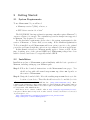
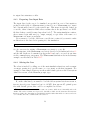
Background
Matpower is a package of Matlab® M-files for solving power flow and optimal
power flow problems. It is intended as a simulation tool for researchers and educators
that is easy to use and modify. Matpower is designed to give the best performance
possible while keeping the code simple to understand and modify. The Matpower
home page can be found at:
http://www.pserc.cornell.edu/matpower/
Matpower was initially developed by Ray D. Zimmerman, Carlos E. MurilloSánchez and Deqiang Gan of PSERC1 at Cornell University under the direction of
Robert J. Thomas. The initial need for Matlab-based power flow and optimal power
flow code was born out of the computational requirements of the PowerWeb project2 .
Many others have contributed to Matpower over the years and it continues to be
developed and maintained under the direction of Ray Zimmerman.
1
2
http://www.pserc.cornell.edu/
http://www.pserc.cornell.edu/powerweb/
9
1.2
License and Terms of Use
Beginning with version 5.1, the code in Matpower is distributed under the 3-clause
BSD license3 [1]. The full text of the license can be found in the LICENSE file at
the top level of the distribution or at http://www.pserc.cornell.edu/matpower/
LICENSE.txt and reads as follows.
Copyright (c) 1996-2015, Power System Engineering Research Center
(PSERC) and individual contributors (see AUTHORS file for details).
All rights reserved.
Redistribution and use in source and binary forms, with or without
modification, are permitted provided that the following conditions
are met:
1. Redistributions of source code must retain the above copyright
notice, this list of conditions and the following disclaimer.
2. Redistributions in binary form must reproduce the above copyright
notice, this list of conditions and the following disclaimer in the
documentation and/or other materials provided with the distribution.
3. Neither the name of the copyright holder nor the names of its
contributors may be used to endorse or promote products derived from
this software without specific prior written permission.
THIS SOFTWARE IS PROVIDED BY THE COPYRIGHT HOLDERS AND CONTRIBUTORS
"AS IS" AND ANY EXPRESS OR IMPLIED WARRANTIES, INCLUDING, BUT NOT
LIMITED TO, THE IMPLIED WARRANTIES OF MERCHANTABILITY AND FITNESS
FOR A PARTICULAR PURPOSE ARE DISCLAIMED. IN NO EVENT SHALL THE
COPYRIGHT HOLDER OR CONTRIBUTORS BE LIABLE FOR ANY DIRECT, INDIRECT,
INCIDENTAL, SPECIAL, EXEMPLARY, OR CONSEQUENTIAL DAMAGES (INCLUDING,
BUT NOT LIMITED TO, PROCUREMENT OF SUBSTITUTE GOODS OR SERVICES;
LOSS OF USE, DATA, OR PROFITS; OR BUSINESS INTERRUPTION) HOWEVER
CAUSED AND ON ANY THEORY OF LIABILITY, WHETHER IN CONTRACT, STRICT
LIABILITY, OR TORT (INCLUDING NEGLIGENCE OR OTHERWISE) ARISING IN
ANY WAY OUT OF THE USE OF THIS SOFTWARE, EVEN IF ADVISED OF THE
POSSIBILITY OF SUCH DAMAGE.
3
Versions 4.0 through 5.0 of Matpower were distributed under version 3.0 of the GNU General
Public License (GPL) [2] with an exception added to clarify our intention to allow Matpower to
interface with Matlab as well as any other Matlab code or MEX-files a user may have installed,
regardless of their licensing terms. The full text of the GPL can be found at http://www.gnu.
org/licenses/gpl-3.0.txt. Matpower versions prior to version 4 had their own license.
10
Please note that the Matpower case files distributed with Matpower are not
covered by the BSD license. In most cases, the data has either been included with
permission or has been converted from data available from a public source.
1.3
Citing Matpower
While not required by the terms of the license, we do request that publications derived
from the use of Matpower explicitly acknowledge that fact by citing reference [3].
R. D. Zimmerman, C. E. Murillo-Sánchez, and R. J. Thomas, “Matpower: SteadyState Operations, Planning and Analysis Tools for Power Systems Research and Education,” Power Systems, IEEE Transactions on, vol. 26, no. 1, pp. 12–19, Feb. 2011.
11
2
Getting Started
2.1
System Requirements
To use Matpower 5.1 you will need:
• Matlab® version 7 (R14) or later4 , or
• GNU Octave version 3.4 or later5
The PSS/E RAW data import function psse2mpc currently requires Matlab 7.3
or newer or Octave 3.8 or newer. The continuation power flow runcpf is not supported
in Matlab 7.0.x (requires 7.1 or newer).
For the hardware requirements, please refer to the system requirements for the
version of Matlab6 or Octave that you are using. If the Matlab Optimization
Toolbox is installed as well, Matpower enables an option to use it to solve optimal
power flow problems, though this option is not recommended for most applications.
In this manual, references to Matlab usually apply to Octave as well. At the
time of writing, none of the optional MEX-based Matpower packages have been
built for Octave, but Octave does typically include GLPK.
2.2
Installation
Installation and use of Matpower requires familiarity with the basic operation of
Matlab, including setting up your Matlab path.
Step 1: Follow the download instructions on the Matpower home page7 . You
should end up with a file named matpowerXXX.zip, where XXX depends on
the version of Matpower.
Step 2: Unzip the downloaded file. Move the resulting matpowerXXX directory to the
location of your choice. These files should not need to be modified, so it is
4
Matlab is available from The MathWorks, Inc. (http://www.mathworks.com/). Matpower 4 required Matlab 6.5 (R13), Matpower 3.2 required Matlab 6 (R12), Matpower 3.0
required Matlab 5 and Matpower 2.0 and earlier required only Matlab 4. Matlab is a registered trademark of The MathWorks, Inc.
5
GNU Octave is free software, available online at http://www.gnu.org/software/octave/.
Some parts of Matpower 5.1 may work on earlier versions of Octave, but it has not been tested
on versions prior to 3.4.
6
http://www.mathworks.com/support/sysreq/previous_releases.html
7
http://www.pserc.cornell.edu/matpower/
12
recommended that they be kept separate from your own code. We will use
$MATPOWER to denote the path to this directory.
13
Step 3: Add the following directories to your Matlab path:
• $MATPOWER – core Matpower functions
• $MATPOWER/t – test scripts for Matpower
• (optional) sub-directories of $MATPOWER/extras – additional functionality and contributed code (see Appendix E for details).
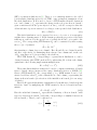
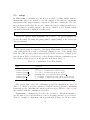
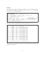
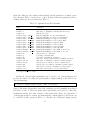
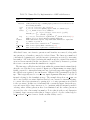
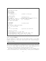
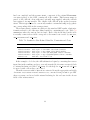
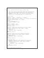
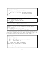
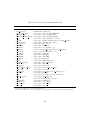
Step 4: At the Matlab prompt, type test matpower to run the test suite and verify
that Matpower is properly installed and functioning. The result should
resemble the following, possibly including extra tests, depending on the
availablility of optional packages, solvers and extras.
14
>> test_matpower
t_nested_struct_copy....ok
t_mpoption..............ok
t_loadcase..............ok
t_ext2int2ext...........ok
t_jacobian..............ok
t_hessian...............ok
t_margcost..............ok
t_totcost...............ok
t_modcost...............ok
t_hasPQcap..............ok
t_mplinsolve............ok
t_mips..................ok
t_qps_matpower..........ok
t_miqps_matpower........ok
t_pf....................ok
t_cpf...................ok
t_islands...............ok
t_opf_model.............ok
t_opf_mips..............ok
t_opf_mips_sc...........ok
t_opf_dc_mips...........ok
t_opf_dc_mips_sc........ok
t_opf_userfcns..........ok
t_opf_softlims..........ok
t_runopf_w_res..........ok
t_dcline................ok
t_get_losses............ok
t_makePTDF..............ok
t_makeLODF..............ok
t_printpf...............ok
t_total_load............ok
t_scale_load............ok
t_psse..................ok
All tests successful (2775
Elapsed time 7.71 seconds.
2.3
(2 of 4 skipped)
(288 of 360 skipped)
(240 of 240 skipped)
(101 of 202 skipped)
(101 of 202 skipped)
passed, 732 skipped of 3507)
Running a Simulation
The primary functionality of Matpower is to solve power flow and optimal power
flow (OPF) problems. This involves (1) preparing the input data defining the all of
the relevant power system parameters, (2) invoking the function to run the simulation
and (3) viewing and accessing the results that are printed to the screen and/or saved
15
in output data structures or files.
2.3.1
Preparing Case Input Data
The input data for the case to be simulated are specified in a set of data matrices
packaged as the fields of a Matlab struct, referred to as a “Matpower case” struct
and conventionally denoted by the variable mpc. This struct is typically defined in
a case file, either a function M-file whose return value is the mpc struct or a MATfile that defines a variable named mpc when loaded8 . The main simulation routines,
whose names begin with run (e.g. runpf, runopf), accept either a file name or a
Matpower case struct as an input.
Use loadcase to load the data from a case file into a struct if you want to make
modifications to the data before passing it to the simulation.
>> mpc = loadcase(casefilename);
See also savecase for writing a Matpower case struct to a case file.
The structure of the Matpower case data is described a bit further in Section 3.1
and the full details are documented in Appendix B and can be accessed at any time
via the command help caseformat. The Matpower distribution also includes many
example case files listed in Table D-17.
2.3.2
Solving the Case
The solver is invoked by calling one of the main simulation functions, such as runpf
or runopf, passing in a case file name or a case struct as the first argument. For
example, to run a simple Newton power flow with default options on the 9-bus system
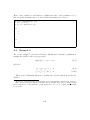
defined in case9.m, at the Matlab prompt, type:
>> runpf('case9');
If, on the other hand, you wanted to load the 30-bus system data from case30.m,
increase its real power demand at bus 2 to 30 MW, then run an AC optimal power
flow with default options, this could be accomplished as follows:
8
This describes version 2 of the Matpower case format, which is used internally and is the
default. The version 1 format, now deprecated, but still accessible via the loadcase and savecase
functions, defines the data matrices as individual variables rather than fields of a struct, and some
do not include all of the columns defined in version 2.
16
>>
>>
>>
>>
define_constants;
mpc = loadcase('case30');
mpc.bus(2, PD) = 30;
runopf(mpc);
The define constants in the first line is simply a convenience script that defines a
number of variables to serve as named column indices for the data matrices. In this
example, it allows us to access the “real power demand” column of the bus matrix
using the name PD without having to remember that it is the 3rd column.
Other top-level simulation functions are available for running DC versions of
power flow and OPF, for running an OPF with the option for Matpower to shut
down (decommit) expensive generators, etc. These functions are listed in Table D-2
in Appendix D.
2.3.3
Accessing the Results
By default, the results of the simulation are pretty-printed to the screen, displaying
a system summary, bus data, branch data and, for the OPF, binding constraint
information. The bus data includes the voltage, angle and total generation and load
at each bus. It also includes nodal prices in the case of the OPF. The branch data
shows the flows and losses in each branch. These pretty-printed results can be saved
to a file by providing a filename as the optional 3rd argument to the simulation
function.
The solution is also stored in a results struct available as an optional return value
from the simulation functions. This results struct is a superset of the Matpower
case struct mpc, with additional columns added to some of the existing data fields
and additional fields. The following example shows how simple it is, after running a
DC OPF on the 118-bus system in case118.m, to access the final objective function
value, the real power output of generator 6 and the power flow in branch 51.
>>
>>
>>
>>
>>
define_constants;
results = rundcopf('case118');
final_objective = results.f;
gen6_output
= results.gen(6, PG);
branch51_flow
= results.branch(51, PF);
Full documentation for the content of the results struct can be found in Sections 4.3 and 6.6.
17
2.3.4
Setting Options
Matpower has many options for selecting among the available solution algorithms,
controlling the behavior of the algorithms and determining the details of the prettyprinted output. These options are passed to the simulation routines as a Matpower
options struct. The fields of the struct have names that can be used to set the
corresponding value via the mpoption function. Calling mpoption with no arguments
returns the default options struct, the struct used if none is explicitly supplied.
Calling it with a set of name and value pairs modifies the default vector.
For example, the following code runs a power flow on the 300-bus example in
case300.m using the fast-decoupled (XB version) algorithm, with verbose printing of
the algorithm progress, but suppressing all of the pretty-printed output.
>> mpopt = mpoption('pf.alg', 'FDXB', 'verbose', 2, 'out.all', 0);
>> results = runpf('case300', mpopt);
To modify an existing options struct, for example, to turn the verbose option off
and re-run with the remaining options unchanged, simply pass the existing options
as the first argument to mpoption.
>> mpopt = mpoption(mpopt, 'verbose', 0);
>> results = runpf('case300', mpopt);
See Appendix C or type:
>> help mpoption
for more information on Matpower’s options.
2.4
Documentation
There are two primary sources of documentation for Matpower. The first is this
manual, which gives an overview of Matpower’s capabilities and structure and
describes the modeling and formulations behind the code. It can be found in your
Matpower distribution at $MATPOWER/docs/manual.pdf.
The second is the built-in help command. As with Matlab’s built-in functions
and toolbox routines, you can type help followed by the name of a command or
M-file to get help on that particular function. Nearly all of Matpower’s M-files
have such documentation and this should be considered the main reference for the
18
calling options for each individual function. See Appendix D for a list of Matpower
functions.
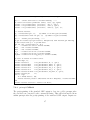
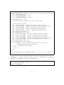
As an example, the help for runopf looks like:
19
>> help runopf
RUNOPF Runs an optimal power flow.
[RESULTS, SUCCESS] = RUNOPF(CASEDATA, MPOPT, FNAME, SOLVEDCASE)
Runs an optimal power flow (AC OPF by default), optionally returning
a RESULTS struct and SUCCESS flag.
Inputs (all are optional):
CASEDATA : either a MATPOWER case struct or a string containing
the name of the file with the case data (default is 'case9')
(see also CASEFORMAT and LOADCASE)
MPOPT : MATPOWER options struct to override default options
can be used to specify the solution algorithm, output options
termination tolerances, and more (see also MPOPTION).
FNAME : name of a file to which the pretty-printed output will
be appended
SOLVEDCASE : name of file to which the solved case will be saved
in MATPOWER case format (M-file will be assumed unless the
specified name ends with '.mat')
Outputs (all are optional):
RESULTS : results struct, with the following fields:
(all fields from the input MATPOWER case, i.e. bus, branch,
gen, etc., but with solved voltages, power flows, etc.)
order - info used in external <-> internal data conversion
et - elapsed time in seconds
success - success flag, 1 = succeeded, 0 = failed
(additional OPF fields, see OPF for details)
SUCCESS : the success flag can additionally be returned as
a second output argument
Calling syntax options:
results = runopf;
results = runopf(casedata);
results = runopf(casedata, mpopt);
results = runopf(casedata, mpopt, fname);
results = runopf(casedata, mpopt, fname, solvedcase);
[results, success] = runopf(...);
Alternatively, for compatibility with previous versions of MATPOWER,
some of the results can be returned as individual output arguments:
[baseMVA, bus, gen, gencost, branch, f, success, et] = runopf(...);
Example:
results = runopf('case30');
See also RUNDCOPF, RUNUOPF.
20
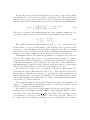
3
Modeling
Matpower employs all of the standard steady-state models typically used for power
flow analysis. The AC models are described first, then the simplified DC models. Internally, the magnitudes of all values are expressed in per unit and angles of complex
quantities are expressed in radians. Internally, all off-line generators and branches
are removed before forming the models used to solve the power flow or optimal power
flow problem. All buses are numbered consecutively, beginning at 1, and generators
are reordered by bus number. Conversions to and from this internal indexing is done
by the functions ext2int and int2ext. The notation in this section, as well as Sections 4 and 6, is based on this internal numbering, with all generators and branches
assumed to be in-service. Due to the strengths of the Matlab programming language in handling matrices and vectors, the models and equations are presented here
in matrix and vector form.
3.1
Data Formats
The data files used by Matpower are Matlab M-files or MAT-files which define
and return a single Matlab struct. The M-file format is plain text that can be edited
using any standard text editor. The fields of the struct are baseMVA, bus, branch, gen
and optionally gencost, where baseMVA is a scalar and the rest are matrices. In the
matrices, each row corresponds to a single bus, branch, or generator. The columns
are similar to the columns in the standard IEEE CDF and PTI formats. The number
of rows in bus, branch and gen are nb , nl and ng , respectively. If present, gencost
has either ng or 2ng rows, depending on whether it includes costs for reactive power
or just real power. Full details of the Matpower case format are documented
in Appendix B and can be accessed from the Matlab command line by typing
help caseformat.
3.2
Branches
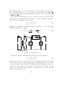
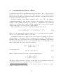
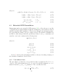
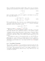
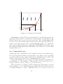
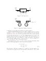
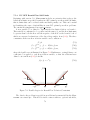
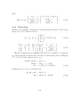
All transmission lines9 , transformers and phase shifters are modeled with a common branch model, consisting of a standard π transmission line model, with series
impedance zs = rs + jxs and total charging susceptance bc , in series with an ideal
phase shifting transformer. The transformer, whose tap ratio has magnitude τ and
9
This does not include DC transmission lines. For more information the handling of DC transmission lines in Matpower, see Section 7.5.3.
21
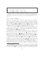
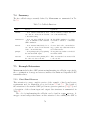
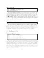
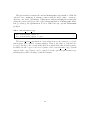
phase shift angle θshift , is located at the from end of the branch, as shown in Figure 3-1. The parameters rs , xs , bc , τ and θshift are specified directly in columns BR R
(3), BR X (4), BR B (5), TAP (9) and SHIFT (10), respectively, of the corresponding row
of the branch matrix.
The complex current injections if and it at the from and to ends of the branch,
respectively, can be expressed in terms of the 2 × 2 branch admittance matrix Ybr
and the respective terminal voltages vf and vt
if
vf
= Ybr
.
(3.1)
it
vt
With the series admittance element in the π model denoted by ys = 1/zs , the branch
admittance matrix can be written
ys + j b2c τ12 −ys τ e−jθ1 shift
.
(3.2)
Ybr =
−ys τ ejθ1shift
ys + j b2c
Figure 3-1: Branch Model
If the four elements of this matrix for branch i are labeled as follows:
i
yff yfi t
i
Ybr =
ytfi ytti
(3.3)
then four nl ×1 vectors Yff , Yf t , Ytf and Ytt can be constructed, where the i-th element
of each comes from the corresponding element of Ybri . Furthermore, the nl ×nb sparse
connection matrices Cf and Ct used in building the system admittance matrices can
be defined as follows. The (i, j)th element of Cf and the (i, k)th element of Ct are
equal to 1 for each branch i, where branch i connects from bus j to bus k. All other
elements of Cf and Ct are zero.
22
3.3
Generators
A generator is modeled as a complex power injection at a specific bus. For generator i,
the injection is
sig = pig + jqgi .
(3.4)
Let Sg = Pg + jQg be the ng × 1 vector of these generator injections. The MW and
MVAr equivalents (before conversion to p.u.) of pig and qgi are specified in columns
PG (2) and QG (3), respectively of row i of the gen matrix. A sparse nb × ng generator
connection matrix Cg can be defined such that its (i, j)th element is 1 if generator j
is located at bus i and 0 otherwise. The nb × 1 vector of all bus injections from
generators can then be expressed as
Sg,bus = Cg · Sg .
3.4
(3.5)
Loads
Constant power loads are modeled as a specified quantity of real and reactive power
consumed at a bus. For bus i, the load is
sid = pid + jqdi
(3.6)
and Sd = Pd + jQd denotes the nb × 1 vector of complex loads at all buses. The
MW and MVAr equivalents (before conversion to p.u.) of pid and qdi are specified in
columns PD (3) and QD (4), respectively of row i of the bus matrix.
Constant impedance and constant current loads are not implemented directly,
but the constant impedance portions can be modeled as a shunt element described
below. Dispatchable loads are modeled as negative generators and appear as negative
values in Sg .
3.5
Shunt Elements
A shunt connected element such as a capacitor or inductor is modeled as a fixed
impedance to ground at a bus. The admittance of the shunt element at bus i is given
as
i
i
= gsh
+ jbish
(3.7)
ysh
and Ysh = Gsh + jBsh denotes the nb × 1 vector of shunt admittances at all buses.
i
The parameters gsh
and bish are specified in columns GS (5) and BS (6), respectively,
of row i of the bus matrix as equivalent MW (consumed) and MVAr (injected) at a
nominal voltage magnitude of 1.0 p.u and angle of zero.
23
3.6
Network Equations
For a network with nb buses, all constant impedance elements of the model are
incorporated into a complex nb × nb bus admittance matrix Ybus that relates the
complex nodal current injections Ibus to the complex node voltages V :
Ibus = Ybus V.
(3.8)
Similarly, for a network with nl branches, the nl × nb system branch admittance
matrices Yf and Yt relate the bus voltages to the nl × 1 vectors If and It of branch
currents at the from and to ends of all branches, respectively:
If = Yf V
It = Yt V.
(3.9)
(3.10)
If [ · ] is used to denote an operator that takes an n × 1 vector and creates the
corresponding n × n diagonal matrix with the vector elements on the diagonal, these
system admittance matrices can be formed as follows:
Yf = [Yff ] Cf + [Yf t ] Ct
Yt = [Ytf ] Cf + [Ytt ] Ct
Ybus = CfT Yf + CtT Yt + [Ysh ] .
(3.11)
(3.12)
(3.13)
The current injections of (3.8)–(3.10) can be used to compute the corresponding
complex power injections as functions of the complex bus voltages V :
∗
∗
Sbus (V ) = [V ] Ibus
= [V ] Ybus
V∗
Sf (V ) = [Cf V ] If∗ = [Cf V ] Yf∗ V ∗
(3.14)
(3.15)
St (V ) = [Ct V ] It∗ = [Ct V ] Yt∗ V ∗ .
(3.16)
The nodal bus injections are then matched to the injections from loads and generators
to form the AC nodal power balance equations, expressed as a function of the complex
bus voltages and generator injections in complex matrix form as
gS (V, Sg ) = Sbus (V ) + Sd − Cg Sg = 0.
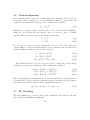
3.7
(3.17)
DC Modeling
The DC formulation [9] is based on the same parameters, but with the following
three additional simplifying assumptions.
24
• Branches can be considered lossless. In particular, branch resistances rs and
charging capacitances bc are negligible:
ys =
1
1
≈
,
rs + jxs
jxs
bc ≈ 0.
(3.18)
• All bus voltage magnitudes are close to 1 p.u.
vi ≈ ejθi .
(3.19)
• Voltage angle differences across branches are small enough that
sin(θf − θt − θshift ) ≈ θf − θt − θshift .
(3.20)
Substituting the first set of assumptions regarding branch parameters from (3.18),
the branch admittance matrix in (3.2) approximates to
1
1
1
−
2
−jθ
shift
τ
τe
Ybr ≈
.
(3.21)
1
jxs − τ ejθ1shift
Combining this and the second assumption with (3.1) yields the following approximation for if :
1
1 1 jθf
( 2 e − −jθ ejθt )
jxs τ
τ e shift
1 1 jθf
=
( e − ej(θt +θshift ) ).
jxs τ τ
if ≈
(3.22)
The approximate real power flow is then derived as follows, first applying (3.19) and
(3.22), then extracting the real part and applying (3.20).
pf = < {sf }
= < vf · i∗f
j 1 −jθf
jθf
−j(θt +θshift )
( e
−e
)
≈< e ·
xs τ τ
j
1
j(θf −θt −θshift )
=<
−e
xs τ τ
1
1
=<
sin(θf − θt − θshift ) + j
− cos(θf − θt − θshift )
xs τ
τ
1
≈
(θf − θt − θshift )
(3.23)
xs τ
25
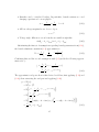
As expected, given the lossless assumption, a similar derivation for the power injection at the to end of the line leads to leads to pt = −pf .
The relationship between the real power flows and voltage angles for an individual
branch i can then be summarized as
pf
θf
i
i
= Bbr
+ Pshift
(3.24)
pt
θt
where
i
Bbr
i
Pshift
1 −1
= bi
,
−1
1
−1
i
= θshift bi
1
and bi is defined in terms of the series reactance xis and tap ratio τ i for branch i as
bi =
1
xis τ i
.
For a shunt element at bus i, the amount of complex power consumed is
i
sish = vi (ysh
vi )∗
i
≈ ejθi (gsh
− jbish )e−jθi
i
= gsh
− jbish .
(3.25)
So the vector of real power consumed by shunt elements at all buses can be approximated by
Psh ≈ Gsh .
(3.26)
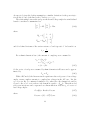
With a DC model, the linear network equations relate real power to bus voltage
angles, versus complex currents to complex bus voltages in the AC case. Let the
nl × 1 vector Bff be constructed similar to Yff , where the i-th element is bi and let
i
Pf,shift be the nl × 1 vector whose i-th element is equal to −θshift
bi . Then the nodal
real power injections can be expressed as a linear function of Θ, the nb × 1 vector of
bus voltage angles
Pbus (Θ) = Bbus Θ + Pbus,shift
(3.27)
where
Pbus,shift = (Cf − Ct )T Pf,shift .
26
(3.28)
Similarly, the branch flows at the from ends of each branch are linear functions of
the bus voltage angles
Pf (Θ) = Bf Θ + Pf,shift
(3.29)
and, due to the lossless assumption, the flows at the to ends are given by Pt = −Pf .
The construction of the system B matrices is analogous to the system Y matrices
for the AC model:
Bf = [Bff ] (Cf − Ct )
T
Bbus = (Cf − Ct ) Bf .
(3.30)
(3.31)
The DC nodal power balance equations for the system can be expressed in matrix
form as
gP (Θ, Pg ) = Bbus Θ + Pbus,shift + Pd + Gsh − Cg Pg = 0
(3.32)
27
4
Power Flow
The standard power flow or loadflow problem involves solving for the set of voltages
and flows in a network corresponding to a specified pattern of load and generation.
Matpower includes solvers for both AC and DC power flow problems, both of
which involve solving a set of equations of the form
g(x) = 0,
(4.1)
constructed by expressing a subset of the nodal power balance equations as functions
of unknown voltage quantities.
All of Matpower’s solvers exploit the sparsity of the problem and, except for
Gauss-Seidel, scale well to very large systems. Currently, none of them include any
automatic updating of transformer taps or other techniques to attempt to satisfy
typical optimal power flow constraints, such as generator, voltage or branch flow
limits.
4.1
AC Power Flow
In Matpower, by convention, a single generator bus is typically chosen as a reference bus to serve the roles of both a voltage angle reference and a real power slack.
The voltage angle at the reference bus has a known value, but the real power generation at the slack bus is taken as unknown to avoid overspecifying the problem.
The remaining generator buses are typically classified as PV buses, with the values
of voltage magnitude and generator real power injection given. These are specified
in the VG (6) and PG (3) columns of the gen matrix, respectively. Since the loads Pd
and Qd are also given, all non-generator buses are classified as PQ buses, with real
and reactive injections fully specified, taken from the PD (3) and QD (4) columns of
the bus matrix. Let Iref , IPV and IPQ denote the sets of bus indices of the reference
bus, PV buses and PQ buses, respectively. The bus type classification is specified in
the Matpower case file in the BUS TYPE column (2) of the bus matrix. Any isolated
buses must be identified as such in this column as well.
In the traditional formulation of the AC power flow problem, the power balance
equation in (3.17) is split into its real and reactive components, expressed as functions
of the voltage angles Θ and magnitudes Vm and generator injections Pg and Qg , where
the load injections are assumed constant and given:
gP (Θ, Vm , Pg ) = Pbus (Θ, Vm ) + Pd − Cg Pg = 0
gQ (Θ, Vm , Qg ) = Qbus (Θ, Vm ) + Qd − Cg Qg = 0.
28
(4.2)
(4.3)
For the AC power flow problem, the function g(x) from (4.1) is formed by taking
the left-hand side of the real power balance equations (4.2) for all non-slack buses
and the reactive power balance equations (4.3) for all PQ buses and plugging in the
reference angle, the loads and the known generator injections and voltage magnitudes:
"
#
{i}
gP (Θ, Vm , Pg )
∀i ∈ IPV ∪ IPQ
g(x) =
(4.4)
{j}
∀j ∈ IPQ .
gQ (Θ, Vm , Qg )
The vector x consists of the remaining unknown voltage quantities, namely the voltage angles at all non-reference buses and the voltage magnitudes at PQ buses:
θ{i}
∀i ∈
/ Iref
x=
(4.5)
{j}
∀j ∈ IPQ .
vm
This yields a system of nonlinear equations with npv + 2npq equations and unknowns, where npv and npq are the number of PV and PQ buses, respectively. After
solving for x, the remaining real power balance equation can be used to compute
the generator real power injection at the slack bus. Similarly, the remaining npv + 1
reactive power balance equations yield the generator reactive power injections.
Matpower includes four different algorithms for solving the AC power flow
problem. The default solver is based on a standard Newton’s method [5] using a
polar form and a full Jacobian updated at each iteration. Each Newton step involves
computing the mismatch g(x), forming the Jacobian based on the sensitivities of
these mismatches to changes in x and solving for an updated value of x by factorizing
this Jacobian. This method is described in detail in many textbooks.
Also included are solvers based on variations of the fast-decoupled method [6],
specifically, the XB and BX methods described in [7]. These solvers greatly reduce
the amount of computation per iteration, by updating the voltage magnitudes and
angles separately based on constant approximate Jacobians which are factored only
once at the beginning of the solution process. These per-iteration savings, however,
come at the cost of more iterations.
The fourth algorithm is the standard Gauss-Seidel method from Glimm and
Stagg [8]. It has numerous disadvantages relative to the Newton method and is
included primarily for academic interest.
By default, the AC power flow solvers simply solve the problem described above,
ignoring any generator limits, branch flow limits, voltage magnitude limits, etc. However, there is an option (pf.enforce q lims) that allows for the generator reactive
power limits to be respected at the expense of the voltage setpoint. This is done
in a rather brute force fashion by adding an outer loop around the AC power flow
29
solution. If any generator has a violated reactive power limit, its reactive injection is
fixed at the limit, the corresponding bus is converted to a PQ bus and the power flow
is solved again. This procedure is repeated until there are no more violations. Note
that this option is based solely on the QMAX and QMIN parameters for the generator,
from columns 4 and 5 of the gen matrix, and does not take into account the trapezoidal generator capability curves described in Section 6.4.3 and specifed in columns
PC1–QC2MAX (11–16).
4.2
DC Power Flow
For the DC power flow problem [9], the vector x consists of the set of voltage angles
at non-reference buses
x = θ{i} , ∀i ∈
/ Iref
(4.6)
and (4.1) takes the form
Bdc x − Pdc = 0
(4.7)
where Bdc is the (nb − 1) × (nb − 1) matrix obtained by simply eliminating from Bbus
the row and column corresponding to the slack bus and reference angle, respectively.
Given that the generator injections Pg are specified at all but the slack bus, Pdc can
be formed directly from the non-slack rows of the last four terms of (3.32).
The voltage angles in x are computed by a direct solution of the set of linear
equations. The branch flows and slack bus generator injection are then calculated
directly from the bus voltage angles via (3.29) and the appropriate row in (3.32),
respectively.
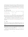
4.3
runpf
In Matpower, a power flow is executed by calling runpf with a case struct or case
file name as the first argument (casedata). In addition to printing output to the
screen, which it does by default, runpf optionally returns the solution in a results
struct.
>> results = runpf(casedata);
The results struct is a superset of the input Matpower case struct mpc, with some
additional fields as well as additional columns in some of the existing data fields.
The solution values are stored as shown in Table 4-1.
Additional optional input arguments can be used to set options (mpopt) and
provide file names for saving the pretty printed output (fname) or the solved case
data (solvedcase).
30
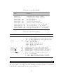
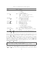
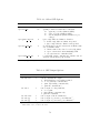
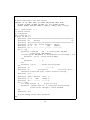
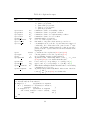
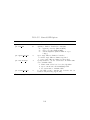
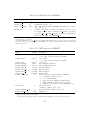
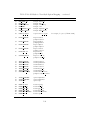
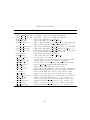
Table 4-1: Power Flow Results
name
description
results.success
results.et
results.order
results.bus(:, VM)†
results.bus(:, VA)
results.gen(:, PG)
results.gen(:, QG)†
results.branch(:, PF)
results.branch(:, PT)
results.branch(:, QF)†
results.branch(:, QT)†
success flag, 1 = succeeded, 0 = failed
computation time required for solution
see ext2int help for details on this field
bus voltage magnitudes
bus voltage angles
generator real power injections
generator reactive power injections
real power injected into “from” end of branch
real power injected into “to” end of branch
reactive power injected into “from” end of branch
reactive power injected into “to” end of branch
†
AC power flow only.
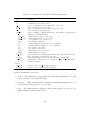
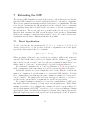
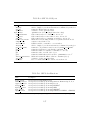
Table 4-2: Power Flow Options
name
default
model
'AC'
pf.alg
'NR'
pf.tol
pf.nr.max it
pf.fd.max it
pf.gs.max it
pf.enforce q lims
10−8
10
30
1000
0
description
AC vs. DC modeling for power flow and OPF formulation
'AC' – use AC formulation and corresponding alg options
'DC' – use DC formulation and corresponding alg options
AC power flow algorithm:
'NR' – Newtons’s method
'FDXB' – Fast-Decoupled (XB version)
'FDBX' – Fast-Decouple (BX version)
'GS' – Gauss-Seidel
termination tolerance on per unit P and Q dispatch
maximum number of iterations for Newton’s method
maximum number of iterations for fast-decoupled method
maximum number of iterations for Gauss-Seidel method
enforce gen reactive power limits at expense of |Vm |
0 – do not enforce limits
1 – enforce limits, simultaneous bus type conversion
2 – enforce limits, one-at-a-time bus type conversion
>> results = runpf(casedata, mpopt, fname, solvedcase);
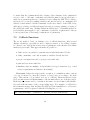
The options that control the power flow simulation are listed in Table 4-2 and those
controlling the output printed to the screen in Table 4-3.
31
By default, runpf solves an AC power flow problem using a standard Newton’s
method solver. To run a DC power flow, the model option must be set to 'DC'. For
convenience, Matpower provides a function rundcpf which is simply a wrapper
that sets the model option to 'DC' before calling runpf.
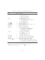
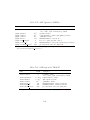
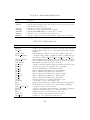
Table 4-3: Power Flow Output Options
name
default
verbose
1
out.all
-1
out.sys sum
out.area sum
out.bus
out.branch
out.gen
out.force
out.suppress detail
1
0
1
1
0
0
-1
†
description
amount of progress info to be printed
0 – print no progress info
1 – print a little progress info
2 – print a lot of progress info
3 – print all progress info
controls pretty-printing of results
-1 – individual flags control what is printed
0 – do not print anything†
1 – print everything†
print system summary (0 or 1)
print area summaries (0 or 1)
print bus detail, includes per bus gen info (0 or 1)
print branch detail (0 or 1)
print generator detail (0 or 1)
print results even if success flag = 0 (0 or 1)
suppress all output but system summary
-1 – suppress details for large systems (> 500 buses)
0 – do not suppress any output specified by other flags
1 – suppress all output except system summary section†
Overrides individual flags, but (in the case of out.suppress detail) not out.all = 1.
Internally, the runpf function does a number of conversions to the problem data
before calling the appropriate solver routine for the selected power flow algorithm.
This external-to-internal format conversion is performed by the ext2int function,
described in more detail in Section 7.2.1, and includes the elimination of out-of-service
equipment, the consecutive renumbering of buses and the reordering of generators
by increasing bus number. All computations are done using this internal indexing.
When the simulation has completed, the data is converted back to external format
by int2ext before the results are printed and returned.
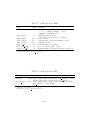
4.4
Linear Shift Factors
The DC power flow model can also be used to compute the sensitivities of branch
flows to changes in nodal real power injections, sometimes called injection shift factors
32
(ISF) or generation shift factors [9]. These nl × nb sensitivity matrices, also called
power transfer distribution factors or PTDFs, carry an implicit assumption about
the slack distribution. If H is used to denote a PTDF matrix, then the element in
row i and column j, hij , represents the change in the real power flow in branch i
given a unit increase in the power injected at bus j, with the assumption that the
additional unit of power is extracted according to some specified slack distribution:
∆Pf = H∆Pbus .
(4.8)
This slack distribution can be expressed as an nb × 1 vector w of non-negative
weights whose elements sum to 1. Each element specifies the proportion of the slack
taken up at each bus. For the special case of a single slack bus k, w is equal to the
vector ek . The corresponding PTDF matrix Hk can be constructed by first creating
the nl × (nb − 1) matrix
ek = B
ef · B −1
H
(4.9)
dc
ef and Bdc are obtained from Bf
then inserting a column of zeros at column k. Here B
and Bbus , respectively, by eliminating their reference bus columns and, in the case
of Bdc , removing row k corresponding to the slack bus.
The PTDF matrix Hw , corresponding to a general slack distribution w, can be
obtained from any other PTDF, such as Hk , by subtracting Hk · w from each column,
equivalent to the following simple matrix multiplication:
Hw = Hk (I − w · 1T ).
(4.10)
These same linear shift factors may also be used to compute sensitivities of branch
flows to branch outages, known as line outage distribution factors or LODFs [10].
Given a PTDF matrix Hw , the corresponding nl × nl LODF matrix L can be constructed as follows, where lij is the element in row i and column j, representing the
change in flow in branch i (as a fraction of the initial flow in branch j) for an outage
of branch j.
First, let H represent the matrix of sensitivities of branch flows to branch endpoint
injections, found by multplying the PTDF matrix by the node-branch incidence
matrix:
H = Hw (Cf − Ct )T .
(4.11)
Here the individual elements hij represent the sensitivity of flow in branch i with
respect to injections at branch j endpoints, corresponding to a simulated increase in
flow in branch j. Then lij can be expressed as

 hij
i 6= j
(4.12)
lij =
1 − hjj

−1
i = j.
33
Matpower includes functions for computing both the DC PTDF matrix and
the corresponding LODF matrix for either a single slack bus k or a general slack
distribution vector w. See the help for makePTDF and makeLODF for details.
34
5
Continuation Power Flow
Continuation methods or branch tracing methods are used to trace a curve given an
initial point on the curve. These are also called predictor-corrector methods since
they involve the prediction of the next solution point and correcting the prediction
to get the next point on the curve.
Consider a system of n nonlinear equations g(x) = 0, x ∈ Rn . By adding a
continuation parameter λ and one more equation to the system, x can be traced by
varying λ. The resulting system f (x, λ) = 0 has n + 1 dimensions. The additional
equation is a parameterized equation which identifies the location of the current
solution with respect to the previous or next solution.
The continuation process can be diagrammatically shown by (5.1).
P redictor
Corrector
xj , λj −−−−−→ (x̂j+1 , λ̂j+1 ) −−−−−→ xj+1 , λj+1
(5.1)
where, (xj , λj ) represents the current solution, (x̂j+1 , λ̂j+1 ) is the predicted solution,
and (xj+1 , λj+1 ) is the next solution on the curve.
Continuation methods are employed in power systems to determine steady state
stability limits [11] in what is called a continuation power flow10 . The limit is determined from a nose curve where the nose represents the maximum power transfer
that the system can handle given a power transfer schedule. To determine the steady
state loading limit, the basic power flow equations
P (x) − P inj
g(x) =
= 0,
(5.2)
Q(x) − Qinj
are restructured as
f (x, λ) = g(x) − λb = 0
where x ≡ (Θ, Vm ) and b is a vector of power transfer given by
inj
inj Ptarget − Pbase
b=
.
inj
Qinj
target − Qbase
(5.3)
(5.4)
The effects of the variation of loading or generation can be investigated using the
continuation method by composing the b vector appropriately.
10
Thanks to Shrirang Abhyankar, Rui Bo, and Alexander Flueck for contributions to Matpower’s continuation power flow feature.
35
5.1
Parameterization
The values of (x, λ) along the solution curve can parameterized in a number of ways
[12, 13]. Parameterization is a mathematical way of identifying each solution so that
the next solution or previous solution can be quantified. Matpower includes three
parameterization scheme options to quantify this relationship, detailed below, where
σ is the continuation step size parameter.
• Natural parameterization simply uses λ directly as the parameter, so the
new λ is simply the previous value plus the step size.
pj (x, λ) = λ − λj − σ = 0
(5.5)
• Arc length parameterization results in the following relationship, where
the step size is equal to the 2-norm of the distance from one solution to the
next.
X
pj (x, λ) =
(xi − xji )2 + (λ − λj )2 − σ 2 = 0
(5.6)
i
• Pseudo arc length parameterization [15] is Matpower’s default parameterization scheme, where the next point (x, λ) on the solution curve is
constrained to lie in the hyperplane running through the predicted solution
(x̂j+1 , λ̂j+1 ) orthogonal to the tangent line from the previous corrected solution
(xj , λj ). This relationship can be quantified by the function
j x
x
j
T
p (x, λ) = z̄j
−
− σ = 0,
(5.7)
λ
λj
where z̄j is the normalized tangent vector at (xj , λj ) and σ is the continuation
step size parameter.
5.2
Predictor
The predictor is used to produce an estimate for the next solution. The better the
prediction, the faster is the convergence to the solution point. Matpower uses a
tangent predictor for estimating the curve to the next solution. The tangent vector
T
zj = dx dλ j at the current solution (xj , λj ) is found by solving the linear
system
fx
fλ
0
zj =
.
(5.8)
j−1
j−1
1
px
pλ
36
The matrix on the left-hand side is simply the standard power flow Jacobian with an
additional column and row added. The extra column fλ is simply the negative of the
power transfer vector b and the extra row, required to make the system non-singular
and define the magnitude of zj , is the derivative of the the parameterization function
at the previous solution point pj−1 .
The resulting tangent vector is then normalized
z̄j =
zj
||zj ||2
(5.9)
and used to compute the predicted approximation (x̂j+1 , λ̂j+1 ) to the next solution
(xj+1 , λj+1 ) using
j+1 j x̂
x
=
+ σz̄j ,
(5.10)
j
j+1
λ
λ̂
where σ is the continuation step size.
5.3
Corrector
The corrector stage finds the next solution (xj+1 , λj+1 ) by correcting the approximation estimated by the predictor (x̂j+1 , λ̂j+1 ). Newton’s method is used to find
the next solution by solving the n + 1 dimensional system in (5.11), where one of
(5.5)–(5.7) has been added as an additional constraint to the parameterized power
flow equations of (5.3).
f (x, λ)
=0
(5.11)
pj (x, λ)
5.4
Step length control
Step length control is a key element affecting the computational efficiency of a continuation method. It affects the continuation method with two issues: (1) speed – how
fast the corrector converges to a specified accuracy, and (2) robustness – whether
the corrector converges to a true solution given a predicted point. Matpower’s
continuation power flow can optionally use adaptive steps, where the step is varied
based on an error estimation between the predicted and corrected solutions as given
in (5.12).
σ n+1 = σ n
cpf
|| (xj+1 , λj+1 ) − x̂j+1 , λ̂j+1 ||∞
37
σmin ≤ σ n+1 ≤ σmax
(5.12)
5.5
runcpf
In Matpower, a continuation power flow is executed by calling runcpf with two
Matpower cases (case structs or case file names) as the first two arguments,
basecasedata and targetcasedata, respectively. The first contains the base loading/generation profile while the second contains the target loading/generation profile. In addition to printing output to the screen, which it does by default, runcpf
optionally returns the solution in a results struct.
>> results = runcpf(basecasedata, targetcasedata);
Additional optional input arguments can be used to set options (mpopt) and
provide file names for saving the pretty printed output (fname) or the solved case
data (solvedcase).
>> results = runcpf(basecasedata, targetcasedata, mpopt, fname, solvedcase);
The results struct is a superset of the input Matpower case struct mpc, with
some additional fields as well as additional columns in some of the existing data
fields. In addition to the solution values included in the results for a simple power
flow, shown in Table 4-1 in Section 4.3, the following additional continuation power
flow solution values are stored in the cpf field as shown in Table 5-1.
Table 5-1: Continuation Power Flow Results
name
description
results.cpf.iterations
results.cpf.lam c
results.cpf.lam p
results.cpf.max lam
results.cpf.V c
results.cpf.V p
nsteps , number of continuation steps performed
1 × n vector of λ values from correction steps†
1 × n vector of λ values from prediction steps†
maximum value of λ found in results.cpf.lam c
nb × n matrix of complex bus voltages from correction steps†
nb × n matrix of complex bus voltages from prediction steps†
†
n is one more than the number of continuation steps, i.e. nsteps + 1.
The options that control the continuation power flow simulation are listed in
Table 5-2. All the power flow options for Newton’s method (tolerance, maximum
iterations) and for controlling the output on the screen (see Tables 4-2 and 4-3) are
also available with the continuation power flow.
Matpower’s continuation power flow also provides a callback mechanism to
give the user access to the iteration process for executing custom code at each iteration, for example, to implement custom incremental plotting of a PV nose curve.
38
Table 5-2: Continuation Power Flow Options
name
cpf.parameterization
cpf.stop at
default
3
'NOSE'
cpf.step
cpf.adapt step
0.05
0
cpf.error tol
cpf.step min
cpf.step max
cpf.plot.level
10−3
10−4
0.2
0
cpf.plot.bus
cpf.user callback
empty
empty
cpf.user callback args
empty
†
description
choice of parameterization
1 — natural
2 — arc length
3 — pseudo arc length
determines stopping criterion
'NOSE' — stop when nose point is reached
'FULL' — trace full nose curve
λstop — stop upon reaching target λ value λstop
continuation power flow step size
toggle adaptive step size feature
0 — adaptive step size disabled
1 — adaptive step size enabled
tolerance for the adaptive step controller
minimum allowed step size
maximum allowed step size
control plotting of nose curve
0 — do not plot nose curve
1 — plot when completed
2 — plot incrementally at each iteration
3 — same as 2, with pause at each iteration
index of bus whose voltage is to be plotted
string or cell array of strings with names of user callback
functions†
struct passed to user-defined callback functions†
See help cpf default callback for details.
Any user-defined callback takes the same input and output arguments as those used
by the cpf default callback function, which is always called and is used to collect the λ and V results from each predictor and corrector iteration. To register
user callback function(s) so it(they) will be executed, the function name(s) is(are)
supplied as a string (cell array of strings) and assigned to the cpf.user callback
option. If your callback requires additional arguments, they can be provided in the
cpf.user callback args option.
The prototype for a CPF user callback function is
function [cb_state, results] = cpf_user_callback(...
k, V_c, lam_c, V_p, lam_p, cb_data, cb_state, cb_args, results)
and the input and output arguments are described in Table 5-3 and in the help for
cpf default callback. The CPF user callback functions are called in three different
39
Table 5-3: Continuation Power Flow Callback Arguments
name
Inputs
k
vc
lam c
vp
lam p
cb data
.mpc base
.mpc target
.Sxfr
.Ybus
.Yf
.Yt
.pv
.pq
.ref
.mpopt
cb state
cb args
results
Ouputs
cb state
results
description
continuation step iteration count
vector of complex bus voltages after k-th corrector step
value of λ after k-th corrector step
vector of complex bus voltages after k-th predictor step
value of λ after k-th predictor step
struct containing potentially useful static data, with the following fields
(all based on internal indexing):
Matpower case struct of base state
Matpower case struct of target state
power transfer vector b from (5.4)
bus admittance matrix
branch admittance matrix, “from” end of branches
branch admittance matrix, “to” end of branches
list of indices of PV buses
list of indices of PQ buses
list of indices of reference buses
Matpower options struct
user-defined struct containing any information the callback function would
like to pass from one invokation to the next
callback arguments struct specified in cpf.user callback args
initial value of output struct to be assigned to cpf field of results struct
returned by runcpf
updated version of cb state input argument
updated version of results input argument
contexts, distinguished as follows:
1. initial – called without results output arg, with input argument k = 0, after
base power flow, before first CPF step.
2. iterations – called without results output arg, with input argument k > 0, at
each iteration, after predictor-corrector step
3. final – called with results output arg, after exiting predictor-corrector loop,
inputs identical to last iteration call
40
Example
The following is an example of running a continuation power flow using a version of
the 9-bus system, looking at increasing all loads by a factor of 2.5. This example
plots the nose curve shown in Figure 5-1.
define_constants;
mpopt = mpoption('out.all', 0, 'verbose', 2);
mpopt = mpoption(mpopt, 'cpf.stop_at', 'FULL', 'cpf.step', 0.2);
mpopt = mpoption(mpopt, 'cpf.plot.level', 2);
mpcb = loadcase(t_case9_pfv2);
% load base case
mpct = mpcb;
% set up target case with
mpct.gen(:, [PG QG]) = mpcb.gen(:, [PG QG]) * 2.5; % increased generation
mpct.bus(:, [PD QD]) = mpcb.bus(:, [PD QD]) * 2.5; % and increased load
results = runcpf(mpcb, mpct, mpopt);
This should result in something like the following output to the screen.
MATPOWER
step
0
step
1
step
2
step
3
step
4
step
5
step
6
step
7
step
8
step
9
step 10
step 11
step 12
step 13
step 14
step 15
Version 5.1, 20-Mar-2015 -- AC Continuation Power Flow
: lambda = 0.000, 4 Newton steps
: lambda = 0.181, 2 corrector Newton steps
: lambda = 0.359, 2 corrector Newton steps
: lambda = 0.530, 2 corrector Newton steps
: lambda = 0.693, 3 corrector Newton steps
: lambda = 0.839, 3 corrector Newton steps
: lambda = 0.952, 3 corrector Newton steps
: lambda = 0.988, 3 corrector Newton steps
: lambda = 0.899, 3 corrector Newton steps
: lambda = 0.776, 3 corrector Newton steps
: lambda = 0.654, 3 corrector Newton steps
: lambda = 0.533, 2 corrector Newton steps
: lambda = 0.413, 2 corrector Newton steps
: lambda = 0.294, 2 corrector Newton steps
: lambda = 0.176, 2 corrector Newton steps
: lambda = 0.000, 3 corrector Newton steps
Traced full continuation curve in 15 continuation steps
The results of the continuation power flow are then found in the cpf field of the
returned results struct.
41
Voltage at Bus 9
1
0.9
0.8
Voltage Magnitude
0.7
0.6
0.5
0.4
0.3
0.2
0.1
0
0
0.1
0.2
0.3
0.4
0.5
λ
0.6
0.7
0.8
0.9
1
Figure 5-1: Nose Curve of Voltage Magnitude at Bus 9
42
>> results.cpf
ans =
V_p:
lam_p:
V_c:
lam_c:
iterations:
max_lam:
[9x16 double]
[1x16 double]
[9x16 double]
[1x16 double]
15
0.9876
43
6
Optimal Power Flow
Matpower includes code to solve both AC and DC versions of the optimal power
flow problem. The standard version of each takes the following form:
min f (x)
x
(6.1)
subject to
g(x) = 0
h(x) ≤ 0
xmin ≤ x ≤ xmax .
6.1
(6.2)
(6.3)
(6.4)
Standard AC OPF
The optimization vector x for the standard AC OPF problem consists of the nb × 1
vectors of voltage angles Θ and magnitudes Vm and the ng × 1 vectors of generator
real and reactive power injections Pg and Qg .


Θ
 Vm 

x=
(6.5)
 Pg 
Qg
The objective function (6.1) is simply a summation of individual polynomial cost
functions fPi and fQi of real and reactive power injections, respectively, for each
generator:
ng
X
fPi (pig ) + fQi (qgi ).
min
(6.6)
Θ,Vm ,Pg ,Qg
i=1
The equality constraints in (6.2) are simply the full set of 2 · nb nonlinear real and
reactive power balance equations from (4.2) and (4.3). The inequality constraints
(6.3) consist of two sets of nl branch flow limits as nonlinear functions of the bus
voltage angles and magnitudes, one for the from end and one for the to end of each
branch:
hf (Θ, Vm ) = |Ff (Θ, Vm )| − Fmax ≤ 0
ht (Θ, Vm ) = |Ft (Θ, Vm )| − Fmax ≤ 0.
44
(6.7)
(6.8)
The flows are typically apparent power flows expressed in MVA, but can be real power
or current flows, yielding the following three possible forms for the flow constraints:


 Sf (Θ, Vm ), apparent power
(6.9)
Ff (Θ, Vm ) = Pf (Θ, Vm ), real power


If (Θ, Vm ), current
where If is defined in (3.9), Sf in (3.15), Pf = <{Sf } and the vector of flow limits
Fmax has the appropriate units for the type of constraint. It is likewise for Ft (Θ, Vm ).
The values used by Matpower’s OPF for the flow limits Fmax are specified in the
RATE A column (6) of the branch matrix.
The variable limits (6.4) include an equality constraint on any reference bus angle
and upper and lower limits on all bus voltage magnitudes and real and reactive
generator injections:
θiref ≤ θi ≤ θiref ,
i,max
i
i,min
,
≤ vm
≤ vm
vm
i,min
i
i,max
pg
≤ pg ≤ pg ,
i,min
≤ qgi ≤ qgi,max ,
qg
i ∈ Iref
i = 1 . . . nb
i = 1 . . . ng
i = 1 . . . ng .
(6.10)
(6.11)
(6.12)
(6.13)
i,min
i,max
are
and vm
The voltage reference angle θiref and voltage magnitude bounds vm
specified in columns VA (9), VMAX (12) and VMIN (13), respectively, of row i of the bus
matrix. Similarly, the generator bounds qgi,max , qgi,min , pi,max
and pi,min
are specfied in
g
g
columns QMAX (4), QMIN (5), PMAX (9) and PMIN (10), respectively, of row i of the gen
matrix.
6.2
Standard DC OPF
When using DC network modeling assumptions and limiting polynomial costs to
second order, the standard OPF problem above can be simplified to a quadratic
program, with linear constraints and a quadratic cost function. In this case, the
voltage magnitudes and reactive powers are eliminated from the problem completely
and real power flows are modeled as linear functions of the voltage angles. The
optimization variable is
Θ
x=
(6.14)
Pg
and the overall problem reduces to the following form.
min
Θ,Pg
ng
X
fPi (pig )
i=1
45
(6.15)
subject to
gP (Θ, Pg ) = Bbus Θ + Pbus,shift + Pd + Gsh − Cg Pg = 0
(6.16)
hf (Θ) = Bf Θ + Pf,shift − Fmax ≤ 0
ht (Θ) = −Bf Θ − Pf,shift − Fmax ≤ 0
(6.17)
(6.18)
θiref ≤ θi ≤ θiref ,
pi,min
≤ pig ≤ pi,max
,
g
g
6.3
i ∈ Iref
i = 1 . . . ng
(6.19)
(6.20)
Extended OPF Formulation
Matpower employs an extensible OPF structure [16] to allow the user to modify
or augment the problem formulation without rewriting the portions that are shared
with the standard OPF formulation. This is done through optional input parameters, preserving the ability to use pre-compiled solvers. The standard formulation is
modified by introducing additional optional user-defined costs fu , constraints, and
variables z and can be written in the following form:
min f (x) + fu (x, z)
(6.21)
g(x) = 0
h(x) ≤ 0
xmin ≤ x ≤ xmax
x
l≤A
≤u
z
zmin ≤ z ≤ zmax .
(6.22)
(6.23)
(6.24)
x,z
subject to
(6.25)
(6.26)
Section 7 describes the mechanisms available to the user for taking advantage of
the extensible formulation described here.
6.3.1
User-defined Costs
The user-defined cost function fu is specified in terms of parameters H, C, N , r̂, k,
d and m. All of the parameters are nw × 1 vectors except the symmetric nw × nw
matrix H and the nw × (nx + nz ) matrix N . The cost takes the form
1
fu (x, z) = wT Hw + C T w
2
46
(6.27)
where w is defined in several steps as follows. First, a new vector u is created by
applying a linear transformation N and shift r̂ to the full set of optimization variables
x
r=N
,
(6.28)
z
u = r − r̂,
(6.29)
then a scaled function with a “dead zone” is applied to each element of u to produce
the corresponding element of w.

ui < −ki
 mi fdi (ui + ki ),
0,
−ki ≤ ui ≤ ki
wi =
(6.30)

mi fdi (ui − ki ),
ui > ki
Here ki specifies the size of the “dead zone”, mi is a simple scale factor and fdi is
a pre-defined scalar function selected by the value of di . Currently, Matpower
implements only linear and quadratic options:
α, if di = 1
fdi (α) =
(6.31)
α2 , if di = 2
as illustrated in Figure 6-1 and Figure 6-2, respectively.
This form for fu provides the flexibility to handle a wide range of costs, from
simple linear functions of the optimization variables to scaled quadratic penalties
on quantities, such as voltages, lying outside a desired range, to functions of linear
combinations of variables, inspired by the requirements of price coordination terms
found in the decomposition of large loosely coupled problems encountered in our own
research.
Some limitations are imposed on the parameters in the case of the DC OPF since
Matpower uses a generic quadratic programming (QP) solver for the optimization.
In particular, ki = 0 and di = 1 for all i, so the “dead zone” is not considered and
only the linear option is available for fdi . As a result, for the DC case (6.30) simplifies
to wi = mi ui .
6.3.2
User-defined Constraints
The user-defined constraints (6.25) are general linear restrictions involving all of the
optimization variables and are specified via matrix A and lower and upper bound
vectors l and u. These parameters can be used to create equality constraints (li = ui )
or inequality constraints that are bounded below (ui = ∞), bounded above (li = ∞)
or bounded on both sides.
47
wi
mi
r̂i
ri
ki
ki
Figure 6-1: Relationship of wi to ri for di = 1 (linear option)
wi
r̂i
ri
ki
ki
Figure 6-2: Relationship of wi to ri for di = 2 (quadratic option)
48
6.3.3
User-defined Variables
The creation of additional user-defined z variables is done implicitly based on the
difference between the number of columns in A and the dimension of x. The optional vectors zmin and zmax are available to impose lower and upper bounds on z,
respectively.
6.4
Standard Extensions
In addition to making this extensible OPF structure available to end users, Matpower also takes advantage of it internally to implement several additional capabilities.
6.4.1
Piecewise Linear Costs
The standard OPF formulation in (6.1)–(6.4) does not directly handle the nonsmooth piecewise linear cost functions that typically arise from discrete bids and
offers in electricity markets. When such cost functions are convex, however, they
can be modeled using a constrained cost variable (CCV) method. The piecewise linear cost function c(x) is replaced by a helper variable y and a set of linear constraints
that form a convex “basin” requiring the cost variable y to lie in the epigraph of the
function c(x).
Figure 6-3 illustrates a convex n-segment piecewise linear cost function


m1 (x − x1 ) + c1 ,
x ≤ x1


 m2 (x − x2 ) + c2 , x1 < x ≤ x2
c(x) =
(6.32)
..
..

.
.


 m (x − x ) + c , x
n
n
n
n−1 < x
defined by a sequence of points (xj , cj ), j = 0 . . . n, where mj denotes the slope of
the j-th segment
cj − cj−1
, j = 1...n
(6.33)
mj =
xj − xj−1
and x0 < x1 < · · · < xn and m1 ≤ m2 ≤ · · · < mn .
The “basin” corresponding to this cost function is formed by the following n
constraints on the helper cost variable y:
y ≥ mj (x − xj ) + cj ,
j = 1 . . . n.
(6.34)
The cost term added to the objective function in place of c(x) is simply the variable y.
49
c
cn
y
c2
c1
c0
x0
x1
x2
xn
x
Figure 6-3: Constrained Cost Variable
Matpower uses this CCV approach internally to automatically generate the
appropriate helper variable, cost term and corresponding set of constraints for any
piecewise linear costs on real or reactive generation. All of Matpower’s OPF
solvers, for both AC and DC OPF problems, use the CCV approach with the exception of two that are part of the optional TSPOPF package [17], namely the
step-controlled primal/dual interior point method (SCPDIPM) and the trust region
based augmented Lagrangian method (TRALM), both of which use a cost smoothing
technique instead [18].
6.4.2
Dispatchable Loads
A simple approach to dispatchable or price-sensitive loads is to model them as negative real power injections with associated negative costs. This is done by specifying
a generator with a negative output, ranging from a minimum injection equal to the
negative of the largest possible load to a maximum injection of zero.
Consider the example of a price-sensitive load whose marginal benefit function is
shown in Figure 6-4. The demand pd of this load will be zero for prices above λ1 , p1
for prices between λ1 and λ2 , and p1 + p2 for prices below λ2 .
This corresponds to a negative generator with the piecewise linear cost curve
shown in Figure 6-5. Note that this approach assumes that the demand blocks can
be partially dispatched or “split”. Requiring blocks to be accepted or rejected in
50
$/MW
λ (marginal benefit)
λ1
p1
λ2
p2
MW
p (load)
Figure 6-4: Marginal Benefit or Bid Function
$
p2
c (total cost)
MW
p (injection)
p1
1
1 p1
2
2 p2
Figure 6-5: Total Cost Function for Negative Injection
51
their entirety would pose a mixed-integer problem that is beyond the scope of the
current Matpower implementation.
With an AC network model, there is also the question of reactive dispatch for
such loads. Typically the reactive injection for a generator is allowed to take on any
value within its defined limits. Since this is not normal load behavior, the model used
in Matpower assumes that dispatchable loads maintain a constant power factor.
When formulating the AC OPF problem, Matpower will automatically generate
an additional equality constraint to enforce a constant power factor for any “negative
generator” being used to model a dispatchable load.
It should be noted that, with this definition of dispatchable loads as negative
generators, if the negative cost corresponds to a benefit for consumption, minimizing
the cost f (x) of generation is equivalent to maximizing social welfare.
6.4.3
Generator Capability Curves
The typical AC OPF formulation includes box constraints on a generator’s real and
reactive injections, specified as simple lower and upper bounds on p (pmin and pmax )
and q (qmin and qmax ). On the other hand, the true P -Q capability curves of physical generators usually involve some tradeoff between real and reactive capability,
so that it is not possible to produce the maximum real output and the maximum
(or minimum) reactive output simultaneously. To approximate this tradeoff, Matpower includes the ability to add an upper and lower sloped portion to the standard
box constraints as illustrated in Figure 6-6, where the shaded portion represents the
feasible operating region for the unit.
The two sloped portions are constructed from the lines passing through the two
pairs of points defined by the six parameters p1 , q1min , q1max , p2 , q2min , and q2max .
If these six parameters are specified for a given generator in columns PC1–QC2MAX
(11–16), Matpower automatically constructs the corresponding additional linear
inequality constraints on p and q for that unit.
If one of the sloped portions of the capability constraints is binding for generator k, the corresponding shadow price is decomposed into the corresponding µPmax
and µQmin or µQmax components and added to the respective column (MU PMAX, MU QMIN
or MU QMAX) in the k th row of gen.
6.4.4
Branch Angle Difference Limits
The difference between the bus voltage angle θf at the from end of a branch and
the angle θt at the to end can be bounded above and below to act as a proxy for a
transient stability limit, for example. If these limits are provided in columns ANGMIN
52
q
q1max
qmax
q2max
p
q2min
qmin
q1min
p1 pmin
pmax
p2
Figure 6-6: Generator P -Q Capability Curve
(12) and ANGMAX (13) of the branch matrix, Matpower creates the corresponding
constraints on the voltage angle variables.11
6.5
Solvers
Early versions of Matpower relied on Matlab’s Optimization Toolbox [19] to
provide the NLP and QP solvers needed to solve the AC and DC OPF problems,
respectively. While they worked reasonably well for very small systems, they did not
scale well to larger networks. Eventually, optional packages with additional solvers
were added to improve performance, typically relying on Matlab extension (MEX)
files implemented in Fortran or C and pre-compiled for each machine architecture.
Some of these MEX files are distributed as optional packages due to differences in
terms of use. For DC optimal power flow, there is a MEX build [20] of the high
11
The voltage angle difference for branch k is taken to be unbounded below if branch(k, ANGMIN)
is less than −360 and unbounded above if branch(k, ANGMAX) is greater than 360. If both parameters are zero, the voltage angle difference is unconstrained.
53
performance interior point BPMPD solver [21] for LP/QP problems. For the AC
OPF problem, the MINOPF [22] and TSPOPF [17] packages provide solvers suitable
for much larger systems. The former is based on MINOS [23] and the latter includes
the primal-dual interior point and trust region based augmented Lagrangian methods
described in [18]. Matpower version 4 and later also includes the option to use the
open-source Ipopt solver12 for solving both AC and DC OPFs, based on the Matlab
MEX interface to Ipopt13 . It also includes the option to use CPLEX14 or MOSEK15
for DC OPFs. Matpower 4.1 added the option to use KNITRO [35]16 for AC OPFs
and the Gurobi Optimizer17 for DC OPFs and Matpower 5 added GLPK and 5.1
added CLP. See Appendix G for more details on these optional packages.
Beginnning with version 4, Matpower also includes its own primal-dual interior
point method implemented in pure-Matlab code, derived from the MEX implementation of the algorithms described in [18]. This solver is called MIPS (Matlab
Interior Point Solver) and is described in more detail in Appendix A. If no optional
packages are installed, MIPS will be used by default for both the AC OPF and as the
QP solver used by the DC OPF. The AC OPF solver also employs a unique technique
for efficiently forming the required Hessians via a few simple matrix operations [24].
This solver has application to general nonlinear optimization problems outside of
Matpower and can be called directly as mips. There is also a convenience wrapper
function called qps mips making it trivial to set up and solve LP and QP problems,
with an interface similar to quadprog from the Matlab Optimization Toolbox.
6.6
runopf
In Matpower, an optimal power flow is executed by calling runopf with a case
struct or case file name as the first argument (casedata). In addition to printing
output to the screen, which it does by default, runpf optionally returns the solution
in a results struct.
>> results = runopf(casedata);
The results struct is a superset of the input Matpower case struct mpc, with
some additional fields as well as additional columns in some of the existing data
12
Available from http://www.coin-or.org/projects/Ipopt.xml.
See https://projects.coin-or.org/Ipopt/wiki/MatlabInterface.
14
See http://www.ibm.com/software/integration/optimization/cplex-optimizer/.
15
See http://www.mosek.com/.
16
See http://www.ziena.com/.
17
See http://www.gurobi.com/.
13
54
fields. In addition to the solution values included in the results for a simple power
flow, shown in Table 4-1 in Section 4.3, the following additional optimal power flow
solution values are stored as shown in Table 6-1.
Table 6-1: Optimal Power Flow Results
name
description
results.f
results.x
results.om
results.bus(:, LAM P)
results.bus(:, LAM Q)
results.bus(:, MU VMAX)
results.bus(:, MU VMIN)
results.gen(:, MU PMAX)
results.gen(:, MU PMIN)
results.gen(:, MU QMAX)
results.gen(:, MU QMIN)
results.branch(:, MU SF)
results.branch(:, MU ST)
results.mu
results.g
results.dg
results.raw
results.var.val
results.var.mu
results.nln
results.lin
results.cost
final objective function value
final value of optimization variables (internal order)
OPF model object†
Lagrange multiplier on real power mismatch
Lagrange multiplier on reactive power mismatch
Kuhn-Tucker multiplier on upper voltage limit
Kuhn-Tucker multiplier on lower voltage limit
Kuhn-Tucker multiplier on upper Pg limit
Kuhn-Tucker multiplier on lower Pg limit
Kuhn-Tucker multiplier on upper Qg limit
Kuhn-Tucker multiplier on lower Qg limit
Kuhn-Tucker multiplier on flow limit at “from” bus
Kuhn-Tucker multiplier on flow limit at “to” bus
shadow prices of constraints‡
(optional) constraint values
(optional) constraint 1st derivatives
raw solver output in form returned by MINOS, and more‡
final value of optimization variables, by named subset‡
shadow prices on variable bounds, by named subset‡
shadow prices on nonlinear constraints, by named subset‡
shadow prices on linear constraints, by named subset‡
final value of user-defined costs, by named subset‡
†
‡
See help for opf model for more details.
See help for opf for more details.
Additional optional input arguments can be used to set options (mpopt) and
provide file names for saving the pretty printed output (fname) or the solved case
data (solvedcase).
>> results = runopf(casedata, mpopt, fname, solvedcase);
Some of the main options that control the optimal power flow simulation are listed
in Tables 6-2 and 6-3. There are many other options that can be used to control the
termination criteria and other behavior of the individual solvers. See Appendix C
or the mpoption help for details. As with runpf the output printed to the screen can
be controlled by the options in Table 4-3, but there are additional output options
55
for the OPF, related to the display of binding constraints that are listed Table 6-4,
along with an option that can be used to force the AC OPF to return information
about the constraint values and Jacobian and the objective function gradient and
Hessian.
By default, runopf solves an AC optimal power flow problem using a primal dual
interior point method. To run a DC OPF, the model option must be set to 'DC'. For
convenience, Matpower provides a function rundcopf which is simply a wrapper
that sets the model to 'DC' before calling runopf.
Internally, the runopf function does a number of conversions to the problem
data before calling the appropriate solver routine for the selected OPF algorithm.
This external-to-internal format conversion is performed by the ext2int function,
described in more detail in Section 7.2.1, and includes the elimination of out-of-service
equipment, the consecutive renumbering of buses and the reordering of generators
by increasing bus number. All computations are done using this internal indexing.
When the simulation has completed, the data is converted back to external format
by int2ext before the results are printed and returned. In addition, both ext2int
and int2ext can be customized via user-supplied callback routines to convert data
needed by user-supplied variables, constraints or costs into internal indexing.
56
Table 6-2: Optimal Power Flow Solver Options
name
default
opf.ac.solver
'DEFAULT'
opf.dc.solver
'DEFAULT'
*
†
‡
description
AC optimal power flow solver:
'DEFAULT' – choose default solver based on availability in
the following order: 'PDIPM', 'MIPS'
'MIPS'
– MIPS, Matlab Interior Point Solver, primal/dual interior point method†
'FMINCON' – Matlab Optimization Toolbox, fmincon
'IPOPT' – Ipopt*
'KNITRO' – KNITRO*
'MINOPF' – MINOPF*, MINOS-based solver
'PDIPM' – PDIPM*, primal/dual interior point method‡
'SDPOPF' – SDPOPF*, solver based on semidefinite relaxation
'TRALM' – TRALM*, trust region based augmented Langrangian method
DC optimal power flow solver:
'DEFAULT' – choose default solver based on availability
in the following order: 'CPLEX', 'GUROBI',
'MOSEK', 'BPMPD', 'OT', 'GLPK' (linear
costs only), 'MIPS'
'MIPS'
– MIPS, Matlab Interior Point Solver, primal/dual interior point method†
'BPMPD' – BPMPD*
'CLP'
– CLP*
'CPLEX' – CPLEX*
'GLPK'
– GLPK*(no quadratic costs)
'GUROBI' – Gurobi*
'IPOPT' – Ipopt*
'MOSEK' – MOSEK*
'OT'
– Matlab Opt Toolbox, quadprog, linprog
Requires the installation of an optional package. See Appendix G for details on the corresponding package.
For MIPS-sc, the step-controlled version of this solver, the mips.step control option must be set to 1.
For SC-PDIPM, the step-controlled version of this solver, the pdipm.step control option must be set to 1.
57
Table 6-3: Other OPF Options
name
default
opf.violation
opf.flow lim
5 × 10−6
'S'
opf.ignore ang lim
0
opf.init from mpc
-1
opf.return raw der
0
†
description
constraint violation tolerance
quantity to limit for branch flow constraints
'S' – apparent power flow (limit in MVA)
'P' – active power flow (limit in MW)
'I' – current magnitude (limit in MVA at 1 p.u.
voltage)
ignore angle difference limits for branches
0 – include angle difference limits, if specified
1 – ignore angle difference limits even if specified
specify whether to use the current state in Matpower
case to initialize OPF†
-1 – Matpower decides based on solver/algorithm
0 – ignore current state when initializing OPF
1 – use current state to initialize OPF
for AC OPF, return constraint and derivative info in
results.raw (in fields g, dg, df, d2f)
Currently supported only for Ipopt, KNITRO and MIPS solvers.
Table 6-4: OPF Output Options
name
default
out.lim.all
-1
out.lim.v
1
out.lim.line
out.lim.pg
out.lim.qg
1
1
1
†
‡
description
controls constraint info output
-1 – individual flags control what is printed
0 – do not print any constraint info†
1 – print only binding constraint info†
2 – print all constraint info†
control output of voltage limit info
0 – do not print
1 – print binding constraints only
2 – print all constraints
control output of line flow limit info‡
control output of gen active power limit info‡
control output of gen reactive power limit info‡
Overrides individual flags.
Takes values of 0, 1 or 2 as for out.lim.v.
58
7
Extending the OPF
The extended OPF formulation described in Section 6.3 allows the user to modify the
standard OPF formulation to include additional variables, costs and/or constraints.
There are two primary mechanisms available for the user to accomplish this. The first
is by directly constructing the full parameters for the addional costs or constraints
and supplying them either as fields in the case struct or directly as arguments to
the opf function. The second, and more powerful, method is via a set of callback
functions that customize the OPF at various stages of the execution. Matpower
includes two examples of using the latter method, one to add a fixed zonal reserve
requirement and another to implement interface flow limits.
7.1
Direct Specification
To add costs directly, the parameters H, C, N , r̂, k, d and m of (6.27)–(6.31)
described in Section 6.3.1 are specified as fields or arguments H, Cw, N and fparm,
repectively, where fparm is the nw × 4 matrix
fparm = d r̂ k m .
(7.1)
When specifying additional costs, N and Cw are required, while H and fparm are
optional. The default value for H is a zero matrix, and the default for fparm is such
that d and m are all ones and r̂ and k are all zeros, resulting in simple linear cost,
with no shift or “dead-zone”. N and H should be specified as sparse matrices.
For additional constraints, the A, l and u parameters of (6.25) are specified as
fields or arguments of the same names, A, l and u, respectively, where A is sparse.
Additional variables are created implicitly based on the difference between the
number of columns in A and the number nx of standard OPF variables. If A has
more columns than x has elements, the extra columns are assumed to correspond to
a new z variable. The initial value and lower and upper bounds for z can also be
specified in the optional fields or arguments, z0, zl and zu, respectively.
For a simple formulation extension to be used for a small number of OPF cases,
this method has the advantage of being direct and straightforward. While Matpower does include code to eliminate the columns of A and N corresponding to Vm
and Qg when running a DC OPF18 , as well as code to reorder and eliminate columns
appropriately when converting from external to internal data formats, this mechanism still requires the user to take special care in preparing the A and N matrices
18
Only if they contain all zeros.
59
to ensure that the columns match the ordering of the elements of the opimization
vectors x and z. All extra constraints and variables must be incorporated into a
single set of parameters that are constructed before calling the OPF. The bookkeeping needed to access the resulting variables and shadow prices on constraints and
variable bounds must be handled manually by the user outside of the OPF, along
with any processing of additional input data and processing, printing or saving of
the additional result data. Making further modifications to a formulation that already includes user-supplied costs, constraints or variables, requires that both sets
be incorporated into a new single consistent set of parameters.
7.2
Callback Functions
The second method, based on defining a set of callback functions, offers several
distinct advantages, especially for more complex scenarios or for adding a feature
for others to use, such as the zonal reserve requirement or the interface flow limits
mentioned previously. This approach makes it possible to:
• define and access variable/constraint sets as individual named blocks
• define constraints, costs only in terms of variables directly involved
• pre-process input data and/or post-process result data
• print and save new result data
• simultaneously use multiple, independently developed extensions (e.g. zonal
reserve requirements and interface flow limits)
Matpower defines five stages in the execution of a simulation where custom
code can be inserted to alter the behavior or data before proceeding to the next
stage. This custom code is defined as a set of “callback” functions that are registered via add userfcn for Matpower to call automatically at one of the five stages.
Each stage has a name and, by convention, the name of a user-defined callback function ends with the name of the corresponding stage. For example, a callback for
the formulation stage that modifies the OPF problem formulation to add reserve
requirements could be registered with the following line of code.
mpc = add_userfcn(mpc, 'formulation', @userfcn_reserves_formulation);
60
The sections below will describe each stage and the input and output arguments
for the corresponding callback function, which vary depending on the stage. An
example that employs additional variables, constraints and costs will be used for
illustration.
Consider the problem of jointly optimizing the allocation of both energy and
reserves, where the reserve requirements are defined as a set of nrz fixed zonal MW
quantities. Let Zk be the set of generators in zone k and Rk be the MW reserve
requirement for zone k. A new set of variables r are introduced representing the
reserves provided by each generator. The value ri , for generator i, must be nonnegative and is limited above by a user-provided upper bound rimax (e.g. a reserve
offer quantity) as well as the physical ramp rate ∆i .
0 ≤ ri ≤ min(rimax , ∆i ),
i = 1 . . . ng
(7.2)
If the vector c contains the marginal cost of reserves for each generator, the user
defined cost term from (6.21) is simply
fu (x, z) = cT r.
(7.3)
There are two additional sets of constraints needed. The first ensures that, for
each generator, the total amount of energy plus reserve provided does not exceed the
capacity of the unit.
pig + ri ≤ pi,max
, i = 1 . . . ng
(7.4)
g
The second requires that the sum of the reserve allocated within each zone k meets
the stated requirements.
X
ri ≥ Rk , k = 1 . . . nrz
(7.5)
i∈Zk
Table 7-1 describes some of the variables and names that are used in the example
callback function listings in the sections below.
7.2.1
ext2int Callback
Before doing any simulation of a case, Matpower performs some data conversion
on the case struct in order to achieve a consistent internal structure, by calling the
following.
mpc = ext2int(mpc);
61
Table 7-1: Names Used by Implementation of OPF with Reserves
name
description
mpc
reserves
Matpower case struct
additional field in mpc containing input parameters for zonal reserves in
the following sub-fields:
ng × 1 vector of reserve costs, c from (7.3)
ng × 1 vector of reserve quantity upper bounds, ith element is rimax
nrz × ng matrixof reserve zone definitions
1 if gen j belongs to reserve zone k (j ∈ Zk )
zones(k,j) =
0 otherwise (j ∈
/ Zk )
nrz × 1 vector of zonal reserve requirements, k th element is Rk from (7.5)
OPF model object, already includes standard OPF setup
OPF results struct, superset of mpc with additional fields for output data
ng , number of generators
name for new reserve variable block, ith element is ri
name for new capacity limit constraint set (7.4)
name for new reserve requirement constraint set (7.5)
cost
qty
zones
req
om
results
ng
R
Pg plus R
Rreq
All isolated buses, out-of-service generators and branches are removed, along with
any generators or branches connected to isolated buses. The buses are renumbered
consecutively, beginning at 1, and the in-service generators are sorted by increasing
bus number. All of the related indexing information and the original data matrices
are stored in an order field in the case struct to be used later by int2ext to perform
the reverse conversions when the simulation is complete.
The first stage callback is invoked from within the ext2int function immediately
after the case data has been converted. Inputs are a Matpower case struct (mpc),
freshly converted to internal indexing and any (optional) args value supplied when
the callback was registered via add userfcn. Output is the (presumably updated)
mpc. This is typically used to reorder any input arguments that may be needed in
internal ordering by the formulation stage. The example shows how e2i field can
also be used, with a case struct that has already been converted to internal indexing,
to convert other data structures by passing in 2 or 3 extra parameters in addition
to the case struct. In this case, it automatically converts the input data in the qty,
cost and zones fields of mpc.reserves to be consistent with the internal generator
ordering, where off-line generators have been eliminated and the on-line generators
are sorted in order of increasing bus number. Notice that it is the second dimension
(columns) of mpc.reserves.zones that is being re-ordered. See the on-line help for
e2i field and e2i data for more details on what all they can do.
62
function mpc = userfcn_reserves_ext2int(mpc, args)
mpc = e2i_field(mpc, {'reserves', 'qty'}, 'gen');
mpc = e2i_field(mpc, {'reserves', 'cost'}, 'gen');
mpc = e2i_field(mpc, {'reserves', 'zones'}, 'gen', 2);
This stage is also a good place to check the consistency of any additional input
data required by the extension and throw an error if something is missing or not as
expected.
7.2.2
formulation Callback
This stage is called from opf after the OPF Model (om) object has been initialized
with the standard OPF formulation, but before calling the solver. This is the ideal
place for modifying the problem formulation with additional variables, constraints
and costs, using the add vars, add constraints and add costs methods of the OPF
Model object. Inputs are the om object and any (optional) args supplied when the
callback was registered via add userfcn. Output is the updated om object.
The om object contains both the original Matpower case data as well as all of the
indexing data for the variables and constraints of the standard OPF formulation.19
See the on-line help for opf model for more details on the OPF model object and the
methods available for manipulating and accessing it.
In the example code, a new variable block named R with ng elements and the
limits from (7.2) is added to the model via the add vars method. Similarly, two
linear constraint blocks named Pg plus R and Rreq, implementing (7.4) and (7.5),
respectively, are added via the add constraints method. And finally, the add costs
method is used to add to the model a user-defined cost block corresponding to (7.3).
Notice that the last argument to add constraints and add costs allows the constraints and costs to be defined only in terms of the relevant parts of the optimization variable x. For example, the A matrix for the Pg plus R constraint contains only
columns corresponding to real power generation (Pg) and reserves (R) and need not
bother with voltages, reactive power injections, etc. As illustrated in Figure 7-1,
this allows the same code to be used with both the AC OPF, where x includes Vm
and Qg , and the DC OPF where it does not. This code is also independent of any
19
It is perfectly legitimate to register more than one callback per stage, such as when enabling
multiple independent OPF extensions. In this case, the callbacks are executed in the order they
were registered with add userfcn. E.g. when the second and subsequent formulation callbacks
are invoked, the om object will reflect any modifications performed by earlier formulation callbacks.
63
additional variables that may have been added by Matpower (e.g. y variables from
Matpower’s CCV handling of piece-wise linear costs) or by the user via previous
formulation callbacks. Matpower will place the constraint matrix blocks in the
appropriate place when it constructs the overall A matrix at run-time. This is an important feature that enables independently developed Matpower OPF extensions
to work together.
A =
Va
Vm
Pg
Qg
y
R
0
0
A1
0
0
A2
Ar =
A =
A1
AC OPF
A2
0
A1
0
A2
Va
Pg
y
R
DC OPF
Figure 7-1: Adding Constraints Across Subsets of Variables
64
function om = userfcn_reserves_formulation(om, args)
%% initialize some things
define_constants;
mpc = get_mpc(om);
r = mpc.reserves;
ng = size(mpc.gen, 1);
%% number of on-line gens
%% variable bounds
Rmin = zeros(ng, 1);
%% bound below by 0
Rmax = r.qty;
%% bound above by stated max reserve qty ...
k = find(mpc.gen(:, RAMP_10) > 0 & mpc.gen(:, RAMP_10) < Rmax);
Rmax(k) = mpc.gen(k, RAMP_10);
%% ... and ramp rate
Rmax = Rmax / mpc.baseMVA;
%% constraints
I = speye(ng);
%% identity matrix
Ar = [I I];
Pmax = mpc.gen(:, PMAX) / mpc.baseMVA;
lreq = r.req / mpc.baseMVA;
%% cost
Cw = r.cost * mpc.baseMVA;
%%
om
om
om
om
%% per unit cost coefficients
add them to the model
= add_vars(om, 'R', ng, [], Rmin, Rmax);
= add_constraints(om, 'Pg_plus_R', Ar, [], Pmax, {'Pg', 'R'});
= add_constraints(om, 'Rreq', r.zones, lreq, [], {'R'});
= add_costs(om, 'Rcost', struct('N', I, 'Cw', Cw), {'R'});
7.2.3
int2ext Callback
After the simulation is complete and before the results are printed or saved, Matpower converts the case data in the results struct back to external indexing by
calling the following.
results = int2ext(results);
This conversion essentially undoes everything that was done by ext2int. Generators
are restored to their original ordering, buses to their original numbering and all
out-of-service or isolated generators, branches and buses are restored.
This callback is invoked from int2ext immediately before the resulting case is
converted from internal back to external indexing. At this point, the simulation
65
has been completed and the results struct, a superset of the original Matpower
case struct passed to the OPF, contains all of the results. This results struct is
passed to the callback, along with any (optional) args supplied when the callback
was registered via add userfcn. The output of the callback is the updated results
struct. This is typically used to convert any results to external indexing and populate
any corresponding fields in the results struct.
The results struct contains, in addition to the standard OPF results, solution information related to all of the user-defined variables, constraints and costs. Table 7-2
summarizes where the various data is found. Each of the fields listed in the table
is actually a struct whose fields correspond to the named sets created by add vars,
add constraints and add costs.
Table 7-2: Results for User-Defined Variables, Constraints and Costs
name
description
results.var.val
results.var.mu.l
results.var.mu.u
results.lin.mu.l
results.lin.mu.u
results.cost
final value of user-defined variables
shadow price on lower limit of user-defined variables
shadow price on upper limit of user-defined variables
shadow price on lower (left-hand) limit of linear constraints
shadow price on upper (right-hand) limit of linear constraints
final value of user-defined costs
In the example code below, the callback function begins by converting the reserves
input data in the resulting case (qty, cost and zones fields of results.reserves) back
to external indexing via calls to i2e field. See the help for i2e field and i2e data
for more details on how they can be used.
Then the reserves results of interest are extracted from the appropriate sub-fields
of results.var, results.lin and results.cost, converted from per unit to per MW
where necessary, and stored with external indexing for the end user in the chosen
fields of the results struct.
66
function results = userfcn_reserves_int2ext(results, args)
%%----- convert stuff back to external indexing ----%% convert all reserve parameters (zones, costs, qty, rgens)
results = i2e_field(results, {'reserves', 'qty'}, 'gen');
results = i2e_field(results, {'reserves', 'cost'}, 'gen');
results = i2e_field(results, {'reserves', 'zones'}, 'gen', 2);
r = results.reserves;
ng = size(results.gen, 1);
%% number of on-line gens (internal)
ng0 = size(results.order.ext.gen, 1);
%% number of gens (external)
%%----- results post-processing ----%% get the results (per gen reserves, multipliers) with internal gen indexing
%% and convert from p.u. to per MW units
[R0, Rl, Ru] = getv(results.om, 'R');
R
= results.var.val.R * results.baseMVA;
Rmin
= Rl * results.baseMVA;
Rmax
= Ru * results.baseMVA;
mu_l
= results.var.mu.l.R / results.baseMVA;
mu_u
= results.var.mu.u.R / results.baseMVA;
mu_Pmax = results.lin.mu.u.Pg_plus_R / results.baseMVA;
%% store in results in results struct
z = zeros(ng0, 1);
results.reserves.R
= i2e_data(results, R, z, 'gen');
results.reserves.Rmin
= i2e_data(results, Rmin, z, 'gen');
results.reserves.Rmax
= i2e_data(results, Rmax, z, 'gen');
results.reserves.mu.l
= i2e_data(results, mu_l, z, 'gen');
results.reserves.mu.u
= i2e_data(results, mu_u, z, 'gen');
results.reserves.mu.Pmax = i2e_data(results, mu_Pmax, z, 'gen');
results.reserves.prc
= z;
for k = 1:ng0
iz = find(r.zones(:, k));
results.reserves.prc(k) = sum(results.lin.mu.l.Rreq(iz)) / results.baseMVA;
end
results.reserves.totalcost = results.cost.Rcost;
7.2.4
printpf Callback
The pretty-printing of the standard OPF output is done via a call to printpf after
the case has been converted back to external indexing. This callback is invoked from
within printpf after the pretty-printing of the standard OPF output. Inputs are
67
the results struct, the file descriptor to write to, a Matpower options struct, and
any (optional) args supplied via add userfcn. Output is the results struct. This is
typically used for any additional pretty-printing of results.
In this example, the out.all flag in the options struct is checked before printing
anything. If it is non-zero, the reserve quantities and prices for each unit are printed
first, followed by the per-zone summaries. An additional table with reserve limit
shadow prices might also be included.
68
function results = userfcn_reserves_printpf(results, fd, mpopt, args)
%% define named indices into data matrices
[GEN_BUS, PG, QG, QMAX, QMIN, VG, MBASE, GEN_STATUS, PMAX, PMIN, ...
MU_PMAX, MU_PMIN, MU_QMAX, MU_QMIN, PC1, PC2, QC1MIN, QC1MAX, ...
QC2MIN, QC2MAX, RAMP_AGC, RAMP_10, RAMP_30, RAMP_Q, APF] = idx_gen;
%%----- print results ----r = results.reserves;
ng = length(r.R);
nrz = size(r.req, 1);
if mpopt.out.all ~= 0
fprintf(fd, '\n=======================================================');
fprintf(fd, '\n|
Reserves
|');
fprintf(fd, '\n=======================================================');
fprintf(fd, '\n Gen
Bus
Status Reserves
Price');
fprintf(fd, '\n #
#
(MW)
($/MW)');
fprintf(fd, '\n---- ----- ------ -------- --------');
for k = 1:ng
fprintf(fd, '\n%3d %6d
%2d ', k, results.gen(k, GEN_BUS), ...
results.gen(k, GEN_STATUS));
if results.gen(k, GEN_STATUS) > 0 && abs(results.reserves.R(k)) > 1e-6
fprintf(fd, '%10.2f', results.reserves.R(k));
else
fprintf(fd, '
- ');
end
fprintf(fd, '%10.2f
', results.reserves.prc(k));
end
fprintf(fd, '\n
--------');
fprintf(fd, '\n
Total:%10.2f
Total Cost: $%.2f', ...
sum(results.reserves.R(r.igr)), results.reserves.totalcost);
fprintf(fd, '\n');
fprintf(fd, '\nZone Reserves
Price ');
fprintf(fd, '\n #
(MW)
($/MW) ');
fprintf(fd, '\n---- -------- --------');
for k = 1:nrz
iz = find(r.zones(k, :));
%% gens in zone k
fprintf(fd, '\n%3d%10.2f%10.2f', k, sum(results.reserves.R(iz)), ...
results.lin.mu.l.Rreq(k) / results.baseMVA);
end
fprintf(fd, '\n');
%% print binding reserve limit multipliers ...
end
69
7.2.5
savecase Callback
The savecase is used to save a Matpower case struct to an M-file, for example,
to save the results of an OPF run. The savecase callback is invoked from savecase
after printing all of the other data to the file. Inputs are the case struct, the file
descriptor to write to, the variable prefix (typically 'mpc.') and any (optional) args
supplied via add userfcn. Output is the case struct. The purpose of this callback is
to write any non-standard case struct fields to the case file.
In this example, the zones, req, cost and qty fields of mpc.reserves are written
to the M-file. This ensures that a case with reserve data, if it is loaded via loadcase,
possibly run, then saved via savecase, will not lose the data in the reserves field.
This callback could also include the saving of the output fields if present. The
contributed serialize function20 can be very useful for this purpose.
20
http://www.mathworks.com/matlabcentral/fileexchange/1206
70
function mpc = userfcn_reserves_savecase(mpc, fd, prefix, args)
%
%
mpc = userfcn_reserves_savecase(mpc, fd, mpopt, args)
%
%
This is the 'savecase' stage userfcn callback that prints the M-file
%
code to save the 'reserves' field in the case file. It expects a
%
MATPOWER case struct (mpc), a file descriptor and variable prefix
%
(usually 'mpc.'). The optional args are not currently used.
r = mpc.reserves;
fprintf(fd, '\n%%%%----- Reserve Data -----%%%%\n');
fprintf(fd, '%%%% reserve zones, element i, j is 1 iff gen j is in zone i\n');
fprintf(fd, '%sreserves.zones = [\n', prefix);
template = '';
for i = 1:size(r.zones, 2)
template = [template, '\t%d'];
end
template = [template, ';\n'];
fprintf(fd, template, r.zones.');
fprintf(fd, '];\n');
fprintf(fd, '\n%%%% reserve requirements for each zone in MW\n');
fprintf(fd, '%sreserves.req = [\t%g', prefix, r.req(1));
if length(r.req) > 1
fprintf(fd, ';\t%g', r.req(2:end));
end
fprintf(fd, '\t];\n');
fprintf(fd, '\n%%%% reserve costs in $/MW for each gen\n');
fprintf(fd, '%sreserves.cost = [\t%g', prefix, r.cost(1));
if length(r.cost) > 1
fprintf(fd, ';\t%g', r.cost(2:end));
end
fprintf(fd, '\t];\n');
if isfield(r, 'qty')
fprintf(fd, '\n%%%% max reserve quantities for each gen\n');
fprintf(fd, '%sreserves.qty = [\t%g', prefix, r.qty(1));
if length(r.qty) > 1
fprintf(fd, ';\t%g', r.qty(2:end));
end
fprintf(fd, '\t];\n');
end
%% save output fields for solved case ...
71
7.3
Registering the Callbacks
As seen in the fixed zonal reserve example, adding a single extension to the standard
OPF formulation is often best accomplished by a set of callback functions. A typical
use case might be to run a given case with and without the reserve requirements
active, so a simple method for enabling and disabling the whole set of callbacks as a
single unit is needed.
The recommended method is to define all of the callbacks in a single file containing
a “toggle” function that registers or removes all of the callbacks depending on whether
the value of the second argument is 'on' or 'off'. The state of the registration of any
callbacks is stored directly in the mpc struct. In our example, the toggle reserves.m
file contains the toggle reserves function as well as the five callback functions.
72
function mpc = toggle_reserves(mpc, on_off)
%TOGGLE_RESERVES Enable, disable or check status of fixed reserve requirements.
%
MPC = TOGGLE_RESERVES(MPC, 'on')
%
MPC = TOGGLE_RESERVES(MPC, 'off')
%
T_F = TOGGLE_RESERVES(MPC, 'status')
if strcmp(upper(on_off), 'ON')
% <code to check for required 'reserves' fields in mpc>
%% add callback functions
mpc = add_userfcn(mpc, 'ext2int', @userfcn_reserves_ext2int);
mpc = add_userfcn(mpc, 'formulation', @userfcn_reserves_formulation);
mpc = add_userfcn(mpc, 'int2ext', @userfcn_reserves_int2ext);
mpc = add_userfcn(mpc, 'printpf', @userfcn_reserves_printpf);
mpc = add_userfcn(mpc, 'savecase', @userfcn_reserves_savecase);
mpc.userfcn.status.dcline = 1;
elseif strcmp(upper(on_off), 'OFF')
mpc = remove_userfcn(mpc, 'savecase', @userfcn_reserves_savecase);
mpc = remove_userfcn(mpc, 'printpf', @userfcn_reserves_printpf);
mpc = remove_userfcn(mpc, 'int2ext', @userfcn_reserves_int2ext);
mpc = remove_userfcn(mpc, 'formulation', @userfcn_reserves_formulation);
mpc = remove_userfcn(mpc, 'ext2int', @userfcn_reserves_ext2int);
mpc.userfcn.status.dcline = 0;
elseif strcmp(upper(on_off), 'STATUS')
if isfield(mpc, 'userfcn') && isfield(mpc.userfcn, 'status') && ...
isfield(mpc.userfcn.status, 'dcline')
mpc = mpc.userfcn.status.dcline;
else
mpc = 0;
end
else
error('toggle_dcline: 2nd argument must be ''on'', ''off'' or ''status''');
end
Running a case that includes the fixed reserves requirements is as simple as
loading the case, turning on reserves and running it.
mpc = loadcase('t_case30_userfcns');
mpc = toggle_reserves(mpc, 'on');
results = runopf(mpc);
73
7.4
Summary
The five callback stages currently defined by Matpower are summarized in Table 7-3.
Table 7-3: Callback Functions
name
invoked . . .
typical use
ext2int
. . . from ext2int immediately after
case data is converted from external
to internal indexing.
Check consistency of input data, convert to internal indexing.
formulation
. . . from opf after OPF Model (om)
object is initialized with standard
OPF formulation.
Modify OPF formulation, by adding
user-defined variables, constraints,
costs.
int2ext
. . . from int2ext immediately before
case data is converted from internal
back to external indexing.
Convert data back to external indexing, populate any additional fields in
the results struct.
printpf
. . . from printpf after pretty-printing
the standard OPF output.
Pretty-print any results not included
in standard OPF.
savecase
. . . from savecase after printing all of
the other case data to the file.
Write non-standard case struct fields
to the case file.
7.5
Example Extensions
Matpower includes three OPF extensions implementing via callbacks, respectively,
the co-optimization of energy and reserves, interface flow limits and dispatchable DC
transmission lines.
7.5.1
Fixed Zonal Reserves
This extension is a more complete version of the example of fixed zonal reserve
requirements used for illustration above in Sections 7.2 and 7.3. The details of
the extensions to the standard OPF problem are given in equations (7.2)–(7.5) and
a description of the relevant input and output data structures is summarized in
Table 7-1.
The code for implementing the callbacks can be found in toggle reserves. A
wrapper around runopf that turns on this extension before running the OPF is
74
provided in runopf w res, allowing you to run a case with an appropriate reserves
field, such as t case30 userfcns, as follows.
results = runopf_w_res('t_case30_userfcns');
See help runopf w res and help toggle reserves for more information. Examples of using this extension and a case file defining the necessary input data can be
found in t opf userfcns and t case30 userfcns, respectively. Additional tests for
runopf w res are included in t runopf w res.
7.5.2
Interface Flow Limits
This extension adds interface flow limits based on flows computed from a DC network
model. It is implemented in toggle iflims. A flow interface k is defined as a set Bk
of branch indices i and a direction for each branch. If pi represents the real power
flow (“from” bus → “to” bus) in branch i and di is equal to 1 or −1 to indicate the
direction,21 then the interface flow fk for interface k is defined as
X
fk (Θ) =
di pi (Θ),
(7.6)
i∈Bk
where each branch flow pi is an approximation calculated as a linear function of the
bus voltage angles based on the DC power flow model from equation (3.29).
This extension adds to the OPF problem a set of nif doubly-bounded constraints
on these flows.
Fkmin ≤ fk (Θ) ≤ Fkmax ∀k ∈ If
(7.7)
where Fkmin and Fkmax are the specified lower and upper bounds on the interface flow,
and If is a the set indices of interfaces whose flow limits are to be enforced.
The data for the problem is specified in an additional if field in the Matpower
case struct mpc. This field is itself a struct with two sub-fields, map and lims, used
for input data, and two others, P and mu, used for output data. The format of this
data is described in detail in Tables 7-4 and 7-5.
See help toggle iflims for more information. Examples of using this extension
and a case file defining the necessary input data for it can be found in t opf userfcns
and t case30 userfcns, respectively. Note that, while this extension can be used for
AC OPF problems, the actual AC interface flows will not necessarily be limited to the
specified values, since it is a DC flow approximation that is used for the constraint.
21
If di = 1, the definitions of the positive flow direction for the branch and the interface are the
same. If di = −1, they are opposite.
75
Table 7-4: Input Data Structures for Interface Flow Limits
name
description
mpc
if
Matpower case struct
additional field in mpc containing input parameters for interface flow limits
inPthe following sub-fields:
( k nk )×2 matrix defining the interfaces, where nk is the number branches
that belong to interface k. The nk branches of interface k are defined by
nk rows in the matrix, where the first column in each is equal to k and
the second is equal to the corresponding branch index i multiplied by di
to indicate the direction.
nif × 3 matrix of interface limits, where nif is the number of interface limits
to be enforced. The first column is the index k of the interface, and the
second and third columns are Fkmin and Fkmax , the lower and upper limits
respectively, on the DC model flow limits (in MW) for the interface.
map
lims
Table 7-5: Output Data Structures for Interface Flow Limits
name
description
results
if
OPF results struct, superset of mpc with additional fields for output data
additional field in results containing output parameters for interface flow
limits in the following sub-fields:
nif × 1 vector of actual flow in MW across the corresponding interface (as
measured at the “from” end of associated branches)
nif × 1 vector of shadow prices on lower flow limits (u/MW)†
nif × 1 vector of shadow prices on upper flow limits (u/MW)†
P
mu.l
mu.u
†
Here we assume the objective function has units u.
Running a case that includes the interface flow limits is as simple as loading the
case, turning on the extension and running it. Unlike with the reserves extension,
Matpower does not currently have a wrapper function to automate this.
mpc = loadcase('t_case30_userfcns');
mpc = toggle_iflims(mpc, 'on');
results = runopf(mpc);
7.5.3
DC Transmission Lines
Beginning with version 4.1, Matpower also includes a simple model for dispatchable
DC transmission lines. While the implementation is based on the extensible OPF
architecture described above, it can be used for simple power flow problems as well,
76
“from”
bus
“to”
bus
DC Line
pf
pt
ploss = l0 + l1 pf
Figure 7-2: DC Line Model
“from”
bus
“to”
bus
pf
pt = (1 − l1 )pf − l0
Figure 7-3: Equivalent “Dummy” Generators
in which the case the (OPF only) formulation callback is skipped.
A DC line in Matpower is modeled as two linked “dummy” generators, as shown
in Figures 7-2 and 7-3, one with negative capacity extracting real power from the
network at the “from” end of the line and another with positive capacity injecting
power into the network at the “to” end. These dummy generators are added by the
ext2int callback and removed by the int2ext callback. The real power flow pf on
the DC line at the “from” end is defined to be equal to the negative of the injection
of corresponding dummy generator. The flow at the “to” end pt is defined to be
equal to the injection of the corresponding generator.
Matpower links the values of pf and pt using the following relationship, which
includes a linear approximation of the real power loss in the line.
pt = pf − ploss
= pf − (l0 + l1 pf )
= (1 − l1 )pf − l0
(7.8)
Here the linear coefficient l1 is assumed to be a small ( 1) positive number. Obviously, this is not applicable for bi-directional lines, where the flow could go either
77
direction, resulting in decreasing losses for increasing flow in the “to” → “from” direction. There are currently two options for handling bi-directional lines. The first
is to use a constant loss model by setting l1 = 0. The second option is to create
two separate but identical lines oriented in opposite directions. In this case, it is
important that the lower limit on the flow and the constant term of the loss model l0
be set to zero to ensure that only one of the two lines has non-zero flow at a time.22
Upper and lower bounds on the value of the flow can be specified for each DC
line, along with an optional operating cost. It is also assumed that the terminals of
the line have a range of reactive power capability that can be used to maintain a
voltage setpoint. Just as with a normal generator, the voltage setpoint is only used
for simple power flow; the OPF dispatches the voltage anywhere between the lower
and upper bounds specified for the bus. Similarly, in a simple power flow the input
value for pf and the corresponding value for pt , computed from (7.8), are used to
specify the flow in the line.
Most of the data for DC lines is stored in a dcline field in the Matpower
case struct mpc. This field is a matrix similar to the branch matrix, where each
row corresponds to a particular DC line. The columns of the matrix are defined in
Table B-5 and include connection bus indices, line status, flows, terminal reactive
injections, voltage setpoints, limits on power flow and VAr injections, and loss parameters. Also, similar to the branch or gen matrices, some of the columns are used
for input values, some for results, and some, such as PF can be either input or output,
depending on whether the problem is a simple power flow or an optimal power flow.
The idx dcline function defines a set of constants for use as named column indices
for the dcline matrix.
An optional dclinecost matrix, in the same form as gencost, can be used to
specify a cost to be applied to pf in the OPF. If the dclinecost field is not present,
the cost is assumed to be zero.
Matpower’s DC line handling is implemented in toggle dcline and examples
of using it can be found in t dcline. The case file t case9 dcline includes some
example DC line data. See help toggle dcline for more information.
Running a case that includes DC lines is as simple as loading the case, turning
on the extension and running it. Unlike with the reserves extension, Matpower
does not currently have a wrapper function to automate this.
mpc = loadcase('t_case9_dcline');
mpc = toggle_dcline(mpc, 'on');
results = runopf(mpc);
22
A future version may make the handling of this second option automatic.
78
7.5.4
DC OPF Branch Flow Soft Limits
Beginning with version 5.0, Matpower includes an extension that replaces the
branch flow limits on specified branches in a DC optimal power flow with soft limits,
that is, limits that can be violated with some linear penalty cost. This can be useful
in identifying the cause of infeasibility in some DC optimal power flow problems.
The extension is implemented in toggle softlims.
A new variable fvi is defined to represent the flow limit violation on branch i.
This variable is constrained to be positive and the sum of fvi and the flow limit must
be greater than both the flow and the negative of the flow on the branch, both of
which are expressed as functions of the bus voltage angles, from (3.29). The three
constraints on the new flow violation variable can be written as
fvi
fvi
+
+
fvi ≥ 0
pi,max
f
pi,max
f
≥
≥
(7.9)
pif
−pif
=
=
Bfi Θ
−Bfi Θ
+
−
pif,shift
pif,shift ,
(7.10)
(7.11)
where the feasible area is illustrated in Figure 7-4. Furthermore, a simple linear cost
coefficient civ is applied to each flow violation variable, so that the additional user
defined cost term from (6.21) looks like
fu (x, z) = cv T fv .
(7.12)
fvi
1
1
pi,max
f
pi,max
f
pif
Figure 7-4: Feasible Region for Branch Flow Violation Constraints
The data for the problem is specifed in an additional softlims field in the Matpower case struct mpc. This field is itself a struct with two optional sub-fields,
79
idx and cost, for input and two others, overload and ovl cost used for output data.
Flow constraint shadow prices are reported in the usual columns of the branch matrix
in the results. The format for this data is detailed in Tables 7-6 and 7-7.
Table 7-6: Input Data Structures for DC OPF Branch Flow Soft Limits
name
description
mpc
softlims
Matpower case struct
additional field in mpc containing input parameters for DC OPF branch
flow soft limits in the following sub-fields:
nsl × 1 vector of branch indices of the branches whose flow limits are to be
converted to soft limits. If empty, it defaults to include all on-line branches
with non-zero branch ratings.
nsl × 1 vector of cost coefficients cv . This is a per MW cost applied to any
flow overload in the corresponding branch. Alternatively, the cost can be
specified as a scalar, in which case it is used for each soft limit. The default
value if not specified is $1000/MW.
idx
cost
Table 7-7: Output Data Structures for DC OPF Branch Flow Soft Limits
name
description
results
OPF results struct, superset of mpc with additional fields for output data
additional field in results containing output parameters for DC
OPF branch flow soft limits in the following sub-fields:
nl × 1 vector of branch flow overloads in MW
nl × 1 vector of branch flow overload penalty costs in u/MW†
for branches whose limits have been replaced with soft limits,
these
contain the Kuhn-Tucker multipliers on the soft limit constraints.‡
softlims
overload
ovl cost
branch(:, MU SF)
branch(:, MU ST)
†
‡
Here we assume the objective function has units u.
When there is no violation of the soft limit, this shadow price is the same as it would be for a hard limit.
When there is a violation, it is equal to the corresponding user-specified constraint violation cost civ .
See help toggle softlims for more information. Examples of using this extension
can be found in t opf softlims. Note that, while this extension can be used for AC
OPF problems, the flow violations will not be actual AC flow violations, since the
computed violations are based on a DC flow model, and it is those values that incur
the penalty cost.
80
Running a case that includes the interface flow limits is as simple as loading the
case, turning on the extension and running it. Unlike with the reserves extension,
Matpower does not currently have a wrapper function to automate this.
mpc = loadcase('case2383wp');
mpc = toggle_softlims(mpc, 'on');
results = rundcopf(mpc);
81
8
Unit De-commitment Algorithm
The standard OPF formulation described in the previous section has no mechanism
for completely shutting down generators which are very expensive to operate. Instead
they are simply dispatched at their minimum generation limits. Matpower includes
the capability to run an optimal power flow combined with a unit de-commitment
for a single time period, which allows it to shut down these expensive units and find
a least cost commitment and dispatch. To run this for case30, for example, type:
>> runuopf('case30')
By default, runuopf is based on the AC optimal power flow problem. To run a DC
OPF, the model option must be set to 'DC'. For convenience, Matpower provides
a function runduopf which is simply a wrapper that sets the model option to 'DC'
before calling runuopf.
Matpower uses an algorithm similar to dynamic programming to handle the
de-commitment. It proceeds through a sequence of stages, where stage N has N
generators shut down, starting with N = 0, as follows:
Step 1: Begin at stage zero (N = 0), assuming all generators are on-line with all
limits in place.
Step 2: If the sum of the minimum generation limits for all on-line generators is less
than the total system demand, then go to Step 3. Otherwise, go to the next
stage, N = N + 1, shut down the generator whose average per-MW cost of
operating at its minimum generation limit is greatest and repeat Step 2.
Step 3: Solve a normal OPF. Save the solution as the current best.
Step 4: Go to the next stage, N = N + 1. Using the best solution from the previous
stage as the base case for this stage, form a candidate list of generators
with minimum generation limits binding. If there are no candidates, skip
to Step 6.
Step 5: For each generator on the candidate list, solve an OPF to find the total
system cost with this generator shut down. Replace the current best solution with this one if it has a lower cost. If any of the candidate solutions
produced an improvement, return to Step 4.
Step 6: Return the current best solution as the final solution.
82
It should be noted that the method employed here is simply a heuristic. It does
not guarantee that the least cost commitment of generators will be found. It is also
rather computationally expensive for larger systems and was implemented as a simple
way to allow an OPF-based “smart-market”, such as described in Appendix F, the
option to reject expensive offers while respecting the minimum generation limits on
generators.
83
9
Miscellaneous Matpower Functions
This section describes a number of additional Matpower functions that users may
find useful. The descriptions here are simply brief summaries, so please use the
Matlab help function to get the full details on each function.
9.1
9.1.1
Input/Output Functions
loadcase
mpc = loadcase(casefile)
The loadcase function provides the canonical way of loading a Matpower case
from a file or struct. It takes as input either a struct or the name of an M-file or
MAT-file in the Matlab path (casefile) and returns a standard Matpower case
struct (mpc). It can also convert from the older version 1 case file format to the
current format. This function allows a case to be loaded, and potentially modified,
before calling one of the main simulation functions such as runpf or runopf.
9.1.2
savecase
savecase(fname, mpc)
savecase(fname, mpc, version)
savecase(fname, comment, mpc)
savecase(fname, comment, mpc, version)
fname = savecase(fname, ...)
The savecase function writes out a Matpower case file, given a name for the
file to be created or overwritten (fname), and a Matpower case struct (mpc). If
fname ends with '.mat' it saves the case as a MAT-file, otherwise it saves it as an
M-file. Optionally returns the filename, with extension added if necessary. The
optional comment argument is either string (single line comment) or a cell array of
strings which are inserted as comments in the help section of the file. If the optional
version argument is '1' it will modify the data matrices to version 1 format before
saving.
84
9.1.3
cdf2mpc
mpc =
mpc =
mpc =
mpc =
[mpc,
cdf2mpc(cdf_file_name)
cdf2mpc(cdf_file_name, verbose)
cdf2mpc(cdf_file_name, mpc_name)
cdf2mpc(cdf_file_name, mpc_name, verbose)
warnings] = cdf2mpc(cdf_file_name, ...)
The cdf2mpc function converts an IEEE Common Data Format (CDF) data file
into a MATPOWER case struct. Given an optional file name mpc name, it can save the
converted case to a Matpower case file. Warnings generated during the conversion
process can be optionally returned in the warnings argument.
Since the IEEE CDF format does not contain all of the data needed to run an
optimal power flow, some data, such as voltage limits, generator limits and generator
costs are created by cdf2mpc. See help cdf2mpc for details.
9.1.4
psse2mpc
mpc =
mpc =
mpc =
mpc =
mpc =
mpc =
[mpc,
psse2mpc(rawfile_name)
psse2mpc(rawfile_name, verbose)
psse2mpc(rawfile_name, verbose, rev)
psse2mpc(rawfile_name, mpc_name)
psse2mpc(rawfile_name, mpc_name, verbose)
psse2mpc(rawfile_name, mpc_name, verbose, rev)
warnings] = psse2mpc(rawfile_name, ...)
The psse2mpc function converts a PSS/E RAW data file into a MATPOWER
case struct. Given an optional file name mpc name, it can save the converted case
to a Matpower case file. Warnings generated during the conversion process can
be optionally returned in the warnings argument. By default, psse2mpc attempts to
determine the revision of the PSS/E RAW file from the contents, but the user can
specify an explicit revision number to use in the optional rev argument.
9.2
9.2.1
System Information
case info
case_info(mpc)
case_info(mpc, fd)
[groups, isolated] = case_info(mpc)
85
The case info function prints out detailed information about a Matpower case,
including connectivity information, summarizing the generation, load and other data
by interconnected island. It can optionally print the output to an open file, whose
file identifier (as returned by fopen) is specified in the optional second parameter fd.
Optional return arguments include groups and isolated buses, as returned by the
find islands function.
9.2.2
compare case
compare_case(mpc1, mpc2)
Compares the bus, branch and gen matrices of two Matpower cases and prints
a summary of the differences. For each column of the matrix it prints the maximum
of any non-zero differences.
9.2.3
find islands
groups = find_islands(mpc)
[groups, isolated] = find_islands(mpc)
The find islands function returns the islands in a network. The return value
groups is a cell array of vectors of the bus indices for each island. The second and
optional return value isolated is a vector of indices of isolated buses that have no
connecting branches.
9.2.4
get losses
loss = get_losses(results)
loss = get_losses(baseMVA, bus, branch)
[loss,
[loss,
[loss,
[loss,
chg] = get_losses(results)
fchg, tchg] = get_losses(results)
fchg, tchg, dloss_dv] = get_losses(results)
fchg, tchg, dloss_dv, dchg_dvm] = get_losses(results)
The get losses function computes branch series losses, and optionally reactive
injections from line charging, as functions of bus voltages and branch parameters,
using the following formulae for a branch, as described in Section 3.2, connecting
bus f to bus t:
86
2
− vt lossi =
rs − jxs
v
2 b
c
f
fchg = jθ shift
τe
2
2 bc
tchg = |vt |
2
vf
τ ejθshift
(9.1)
(9.2)
(9.3)
It can also optionally compute the partial derivatives of the line losses and reactive
charging injections with respect to voltage angles and magnitudes.
9.2.5
margcost
marginalcost = margcost(gencost, Pg)
The margcost function computes the marginal cost for generators given a matrix
in gencost format and a column vector or matrix of generation levels. The return
value has the same dimensions as Pg. Each row of gencost is used to evaluate the cost
at the output levels specified in the corresponding row of Pg. The rows of gencost
can specify either polynomial or piecewise linear costs and need not be uniform.
9.2.6
isload
TorF = isload(gen)
The isload function returns a column vector of 1’s and 0’s. The 1’s correspond
to rows of the gen matrix which represent dispatchable loads. The current test is
Pmin < 0 and Pmax = 0.
9.2.7
printpf
printpf(results, fd, mpopt)
The printpf function prints power flow and optimal power flow results, as returned to fd, a file identifier which defaults to STDOUT (the screen). The details of
what gets printed are controlled by an optional Matpower options struct mpopt.
87
9.2.8
total load
Pd = total_load(bus)
Pd = total_load(bus, gen, load_zone, opt)
[Pd, Qd] = total_load(...)
The total load function returns a vector of total load in each load zone. The
opt argument controls whether it includes fixed loads, dispatchable loads or both,
and for dispatchable loads, whether to use the nominal or realized load values. The
load zone argument defines the load zones across which loads will be summed. It
uses the BUS AREA column (7) of the bus matrix by default. The string value 'all' can
be used to specify a single zone including the entire system. The reactive demands
are also optionally available as an output.
9.2.9
totcost
totalcost = totcost(gencost, Pg)
The totcost function computes the total cost for generators given a matrix in
gencost format and a column vector or matrix of generation levels. The return value
has the same dimensions as Pg. Each row of gencost is used to evaluate the cost at
the output levels specified in the corresponding row of Pg. The rows of gencost can
specify either polynomial or piecewise linear costs and need not be uniform.
9.3
9.3.1
Modifying a Case
extract islands
mpc_array = extract_islands(mpc)
mpc_array = extract_islands(mpc, groups)
mpc_k = extract_islands(mpc, k)
mpc_k = extract_islands(mpc, groups, k)
mpc_k = extract_islands(mpc, k, custom)
mpc_k = extract_islands(mpc, groups, k, custom)
The extract islands function extracts individual islands in a network that is not
fully connected. The original network is specified as a Matpower case struct (mpc)
and the result is returned as a cell array of case structs, or as a single case struct.
Supplying the optional group avoids the need to traverse the network again, saving
time on large systems. A final optional argument custom is a struct that can be used
to indicate custom fields of mpc from which to extract data corresponding to buses
generators, branches or DC lines.
88
9.3.2
mpc
mpc
mpc
mpc
load2disp
=
=
=
=
load2disp(mpc0);
load2disp(mpc0, fname);
load2disp(mpc0, fname, idx);
load2disp(mpc0, fname, idx, voll);
The load2disp function takes a Matpower case mpc0, converts fixed loads to
dispatchable loads, curtailable at a specific price, and returns the resulting case
struct mpc. It can optionally save the resulting case to a file (fname), convert loads
only at specific buses (idx), and set the value of lost load (voll) to be used as the
curtailment price (default is $5,000/MWh).
9.3.3
modcost
newgencost = modcost(gencost, alpha)
newgencost = modcost(gencost, alpha, modtype)
The modcost function can be used to modify generator cost functions by shifting
or scaling them, either horizontally or vertically. The alpha argument specifies the
numerical value of the modification, and modtype defines the type of modification
as a string that takes one of the following values: 'SCALE F' (default), 'SCALE X',
'SHIFT F', or 'SHIFT X'.
9.3.4
scale load
bus = scale_load(load, bus);
[bus, gen] = scale_load(load, bus, gen, load_zone, opt)
[bus, gen, gencost] = ...
scale_load(load, bus, gen, load_zone, opt, gencost)
The scale load function is used to scale active (and optionally reactive) loads in
each zone by a zone-specific ratio, i.e. R(k) for zone k. The amount of scaling for
each zone, either as a direct scale factor or as a target quantity, is specified in load.
The load zones are defined by load zone, and opt specifies the type of scaling (factor
or target quantity) and which loads are affected (active, reactive or both and fixed,
dispatchable or both). The costs (gencost) associated with dispatchable loads can
also be optionally scaled with the loads.
89
9.4
9.4.1
Conversion between External and Internal Numbering
ext2int, int2ext
mpc_int = ext2int(mpc_ext)
mpc_ext = int2ext(mpc_int)
These functions convert a Matpower case struct from external to internal, and
from internal to external numbering, respectively. ext2int first removes all isolated
buses, off-line generators and branches, and any generators or branches connected
to isolated buses. Then the buses are renumbered consecutively, beginning at 1,
and the generators are sorted by increasing bus number. Any 'ext2int' callback
routines registered in the case are also invoked automatically. All of the related
indexing information and the original data matrices are stored in an 'order' field in
the struct to be used later by codeint2ext to perform the reverse conversions. If the
case is already using internal numbering it is returned unchanged.
9.4.2
val
val
val
val
e2i data, i2e data
=
=
=
=
e2i_data(mpc,
e2i_data(mpc,
i2e_data(mpc,
i2e_data(mpc,
val,
val,
val,
val,
ordering)
ordering, dim)
oldval, ordering)
oldval, ordering, dim)
These functions can be used to convert other data structures from external to
internal indexing and vice versa. When given a case struct (mpc) that has already
been converted to internal indexing, e2i data can be used to convert other data
structures as well by passing in 2 or 3 extra parameters in addition to the case
struct. If the value passed in the second argument (val) is a column vector or cell
array, it will be converted according to the ordering specified by the third argument
(described below). If val is an n-dimensional matrix or cell array, then the optional
fourth argument (dim, default = 1) can be used to specify which dimension to reorder.
The return value in this case is the value passed in, converted to internal indexing.
The third argument, ordering, is used to indicate whether the data corresponds
to bus-, gen- or branch-ordered data. It can be one of the following three strings:
'bus', 'gen' or 'branch'. For data structures with multiple blocks of data, ordered
by bus, gen or branch, they can be converted with a single call by specifying ordering
as a cell array of strings.
Any extra elements, rows, columns, etc. beyond those indicated in ordering, are
not disturbed.
90
The function i2e data performs the opposite conversion, from internal back to
external indexing. It also assumes that mpc is using internal indexing, and the only
difference is that it also includes an oldval argument used to initialize the return
value before converting val to external indexing. In particular, any data corresponding to off-line gens or branches or isolated buses or any connected gens or branches
will be taken from oldval, with val supplying the rest of the returned data.
9.4.3
mpc
mpc
mpc
mpc
e2i field, i2e field
=
=
=
=
e2i_field(mpc,
e2i_field(mpc,
i2e_field(mpc,
i2e_field(mpc,
field,
field,
field,
field,
ordering)
ordering, dim)
ordering)
ordering, dim)
These functions can be used to convert additional fields in mpc from external to
internal indexing and vice versa. When given a case struct that has already been
converted to internal indexing, e2i field can be used to convert other fields as well
by passing in 2 or 3 extra parameters in addition to the case struct.
The second argument (field) is a string or cell array of strings, specifying a
field in the case struct whose value should be converted by a corresponding call to
e2i data. The field can contain either a numeric or a cell array. The converted value
is stored back in the specified field, the original value is saved for later use and the
updated case struct is returned. If field is a cell array of strings, they specify nested
fields.
The third and optional fourth arguments (ordering and dim) are simply passed
along to the call to e2i data.
Similarly, i2e field performs the opposite conversion, from internal back to external indexing. It also assumes that mpc is using internal indexing and utilizes the
original data stored by e2i field, calling i2e data to do the conversion work.
9.5
9.5.1
Forming Standard Power Systems Matrices
makeB
[Bp, Bpp] = makeB(baseMVA, bus, branch, alg)
The makeB function builds the two matrices B 0 and B 00 used in the fast-decoupled
power flow. The alg, which can take values 'FDXB' or 'FDBX', determines whether
the matrices returned correspond to the XB or BX version of the fast-decoupled
power flow.
91
9.5.2
makeBdc
[Bbus, Bf, Pbusinj, Pfinj] = makeBdc(baseMVA, bus, branch)
The function builds the B matrices, Bdc (Bbus) and Bf (Bf), and phase shift injections, Pdc (Pbusinj) and Pf,shift (Pfinj), for the DC power flow model as described
in (3.29) and (4.7).
9.5.3
makeJac
J = makeJac(mpc)
J = makeJac(mpc, fullJac)
[J, Ybus, Yf, Yt] = makejac(mpc)
The makeJac function forms the power flow Jacobian and, optionally, the system
admittance matrices. Bus numbers in the input case must be consecutive beginning
at 1 (i.e. internal indexing). If the fullJac argument is present and true, it returns
the full Jacobian (sensitivities of all bus injections with respect to all voltage angles
and magnitudes) as opposed to the reduced version used in the Newton power flow
updates.
9.5.4
makeYbus
[Ybus, Yf, Yt] = makeYbus(mpc)
[Ybus, Yf, Yt] = makeYbus(baseMVA, bus, branch)
The makeYbus function builds the bus admittance matrix and branch admittance
matrices from (3.11)–(3.13). Bus numbers in the input case must be consecutive
beginning at 1 (i.e. internal indexing).
9.6
9.6.1
Miscellaneous
define constants
define_constants
The define constants is a convenience script that defines a set of constants to be
used as named column indices into the bus, branch, gen and gencost data matrices.
The purpose is to avoid having to remember column numbers and to allow code to be
more robust against potential future changes to the Matpower case data format.
92
9.6.2
have fcn
TorF = have_fcn(tag)
TorF = have_fcn(tag, toggle)
ver_str = have_fcn(tag, 'vstr')
ver_num = have_fcn(tag, 'vnum')
rdate
= have_fcn(tag, 'date')
info
= have_fcn(tag, 'all')
The have fcn function provides a unified mechanism for testing for optional functionality, such as the presence of certain solvers, or to detect whether the code is
running under Matlab or Octave. Since its results are cached they allow for a very
quick way to check frequently for functionality that may initially be a bit more costly
to determine. For installed functionality, have fcn also determines the installed version and release date, if possible. The optional second argument, when it is a string,
defines which value is returned, as follows:
• empty – 1 if optional functionality is available, 0 if not available
• 'vstr' – version number as a string (e.g. '3.11.4')
• 'vnum' – version number as numeric value (e.g. 3.011004)
• 'date' – release date as a string (e.g. '20-Jan-2015')
• 'all' – struct with fields named av (for “availability”), vstr, vnum and date,
and values corresponding to each of the above, respectively.
Alternatively, the optional functionality specified by tag can be toggled OFF or
ON by calling have fcn with a numeric second argument toggle with one of the
following values:
• 0 – turn OFF the optional functionality
• 1 – turn ON the optional functionality (if available)
• −1 – toggle the ON/OFF state of the optional functionality
9.6.3
mpver
mpver
v = mpver
v = mpver('all')
93
The mpver function returns the current Matpower version number. With the
optional 'all' argument, it returns a struct with the fields 'Name', 'Version',
'Release' and 'Date' (all strings). Calling mpver without assigning the return value
prints the version and release date of the current installation of Matpower, Matlab (or Octave), the Optimization Toolbox, MIPS and any optional Matpower
packages.
9.6.4
nested struct copy
ds = nested_struct_copy(d, s)
ds = nested_struct_copy(d, s, opt)
The nested struct copy function copies values from a source struct s to a destination struct d in a nested, recursive manner. That is, the value of each field in s
is copied directly to the corresponding field in d, unless that value is itself a struct,
in which case the copy is done via a recursive call to nested struct copy. Certain
aspects of the copy behavior can be controled via the optional options struct opt,
including the possible checking of valid field names.
94
10
Acknowledgments
The authors would like to acknowledge contributions from others who have helped
make Matpower what it is today. First we would like to acknowledge the input
and support of Bob Thomas throughout the development of Matpower. Thanks to
Chris DeMarco, one of our PSERC associates at the University of Wisconsin, for the
technique for building the Jacobian matrix. Our appreciation to Bruce Wollenberg
for all of his suggestions for improvements to version 1. The enhanced output functionality in version 2.0 is primarily due to his input. Thanks also to Andrew Ward
for code which helped us verify and test the ability of the OPF to optimize reactive
power costs. Thanks to Alberto Borghetti for contributing code for the Gauss-Seidel
power flow solver and to Mu Lin for contributions related to power flow reactive
power limits. Real power line limits were suggested by Pan Wei. Thanks to Roman
Korab for data for the Polish system. Some state estimation code was contributed
by James S. Thorp and Rui Bo contributed additional code for state estimation and
continuation power flow. Matpower was improved in various ways in response to
Doug Mitarotonda’s contributions and suggestions.
Thanks also to many others who have contributed code, testing time, bug reports
and suggestions over the years. And, last but not least, thanks to all of the many
users who, by using Matpower in their own work, have helped to extend the
contribution of Matpower to the field of power systems far beyond what we could
do on our own.
95
Appendix A
MIPS – Matlab Interior Point Solver
Beginning with version 4, Matpower includes a new primal-dual interior point
solver called MIPS, for Matlab Interior Point Solver. It is implemented in pureMatlab code, derived from the MEX implementation of the algorithms described
in [18, 25].
This solver has application outside of Matpower to general nonlinear optimization problems of the following form:
min f (x)
(A.1)
g(x) = 0
h(x) ≤ 0
l ≤ Ax ≤ u
xmin ≤ x ≤ xmax
(A.2)
(A.3)
(A.4)
(A.5)
x
subject to
where f : Rn → R, g : Rn → Rm and h : Rn → Rp .
The solver is implemented by the mips function, which can be called as follows,
[x, f, exitflag, output, lambda] = ...
mips(f_fcn, x0, A, l, u, xmin, xmax, gh_fcn, hess_fcn, opt);
where the input and output arguments are described in Tables A-1 and A-2, respectively. Alternatively, the input arguments can be packaged as fields in a problem
struct and passed in as a single argument, where all fields except f fcn and x0 are
optional.
[x, f, exitflag, output, lambda] = mips(problem);
The calling syntax is nearly identical to that used by fmincon from Matlab’s
Optimization Toolbox. The primary difference is that the linear constraints are
specified in terms of a single doubly-bounded linear function (l ≤ Ax ≤ u) as opposed
to separate equality constrained (Aeq x = beq ) and upper bounded (Ax ≤ b) functions.
Internally, equality constraints are handled explicitly and determined at run-time
based on the values of l and u.
The user-defined functions for evaluating the objective function, constraints and
Hessian are identical to those required by fmincon, with one exception described
96
Table A-1: Input Arguments for mips†
name
description
f fcn
Handle to a function that evaluates the objective function, its gradients and Hessian‡
for a given value of x. Calling syntax for this function:
[f, df, d2f] = f fcn(x)
Starting value of optimization vector x.
Define the optional linear constraints l ≤ Ax ≤ u. Default values for the elements of
l and u are -Inf and Inf, respectively.
Optional lower and upper bounds on the x variables, defaults are -Inf and Inf,
respectively.
Handle to function that evaluates the optional nonlinear constraints and their gradients for a given value of x. Calling syntax for this function is:
[h, g, dh, dg] = gh fcn(x)
Handle to function that computes the Hessian‡ of the Lagrangian for given values
of x, λ and µ, where λ and µ are the multipliers on the equality and inequality
constraints, g and h, respectively. The calling syntax for this function is:
Lxx = hess fcn(x, lam, cost mult),
where λ = lam.eqnonlin, µ = lam.ineqnonlin and cost mult is a parameter used
to scale the objective function
Optional options structure with fields, all of which are also optional, described in
Table A-3.
Alternative, single argument input struct with fields corresponding to arguments
above.
x0
A, l, u
xmin, xmax
gh fcn
hess fcn
opt
problem
†
‡
All inputs are optional except f fcn and x0.
If gh fcn is provided then hess fcn is also required. Specifically, if there are nonlinear constraints, the Hessian
information must provided by the hess fcn function and it need not be computed in f fcn.
below for the Hessian evaluation function. Specifically, f fcn should return f as the
scalar objective function value f (x), df as an n × 1 vector equal to ∇f and, unless
gh fcn is provided and the Hessian is computed by hess fcn, d2f as an n × n matrix
2
equal to the Hessian ∂∂xf2 . Similarly, the constraint evaluation function gh fcn must
return the m × 1 vector of nonlinear equality constraint violations g(x), the p × 1
vector of nonlinear inequality constraint violations h(x) along with their gradients
in dg and dh. Here dg is an n × m matrix whose j th column is ∇gj and dh is n × p,
with j th column equal to ∇hj . Finally, for cases with nonlinear constraints, hess fcn
2
returns the n × n Hessian ∂∂xL2 of the Lagrangian function
L(x, λ, µ, σ) = σf (x) + λT g(x) + µT h(x)
(A.6)
for given values of the multipliers λ and µ, where σ is the cost mult scale factor for
the objective function. Unlike fmincon, mips passes this scale factor to the Hessian
evaluation function in the 3rd argument.
97
Table A-2: Output Arguments for mips
name
description
x
f
exitflag
solution vector
final objective function value
exit flag
1 – first order optimality conditions satisfied
0 – maximum number of iterations reached
-1 – numerically failed
output struct with fields
iterations number of iterations performed
hist
struct array with trajectories of the following: feascond,
gradcond, compcond, costcond, gamma, stepsize, obj, alphap,
alphad
message
exit message
struct containing the Langrange and Kuhn-Tucker multipliers on the constraints, with fields:
eqnonlin
nonlinear equality constraints
ineqnonlin nonlinear inequality constraints
lower (left-hand) limit on linear constraints
mu l
mu u
upper (right-hand) limit on linear constraints
lower
lower bound on optimization variables
upper
upper bound on optimization variables
output
lambda
The use of nargout in f fcn and gh fcn is recommended so that the gradients
and Hessian are only computed when required.
A.1
Example 1
The following code shows a simple example of using mips to solve a 2-dimensional
unconstrained optimization of Rosenbrock’s “banana” function23
f (x) = 100(x2 − x21 )2 + (1 − x1 )2 .
(A.7)
First, create a Matlab function that will evaluate the objective function, its
gradients and Hessian, for a given value of x. In this case, the coefficient of the first
term is defined as a paramter a.
23
http://en.wikipedia.org/wiki/Rosenbrock_function
98
Table A-3: Options for mips†
name
opt.verbose
opt.feastol
opt.gradtol
opt.comptol
opt.costtol
opt.max it
opt.step control
opt.sc.red it
opt.cost mult
opt.xi
opt.sigma
opt.z0
opt.alpha min
default
0
10−6
10−6
10−6
10−6
150
0
20
1
0.99995
0.1
1
10−8
opt.rho min
opt.rho max
opt.mu threshold
0.95
1.05
10−5
opt.max stepsize
1010
description
controls level of progress output displayed
0 – print no progress info
1 – print a little progress info
2 – print a lot of progress info
3 – print all progress info
termination tolerance for feasibility condition
termination tolerance for gradient condition
termination tolerance for complementarity condition
termination tolerance for cost condition
maximum number of iterations
set to 1 to enable step-size control
max number of step-size reductions if step-control is on
cost multiplier used to scale the objective function for improved
conditioning. Note: This value is also passed as the 3rd argument to the Hessian evaluation function so that it can appropriately scale the objective function term in the Hessian of the
Lagrangian.
ξ constant used in α updates in (A.46) and (A.47)
centering parameter σ used in γ update in (A.52)
used to initialize elements of slack variable Z
algorithm returns “Numerically Failed” if the αp or αd from
(A.46) and (A.47) become smaller than this value
lower bound on ρt corresponding to 1 − η in Fig. 5 in [18]
upper bound on ρt corresponding to 1 + η in Fig. 5 in [18]
Kuhn-Tucker multipliers smaller than this value for non-binding
constraints are forced to zero
algorithm returns “Numerically Failed” if the 2-norm of the New∆X
ton step
from (A.45) exceeds this value
∆λ
function [f, df, d2f] = banana(x, a)
f = a*(x(2)-x(1)^2)^2+(1-x(1))^2;
if nargout > 1
%% gradient is required
df = [ 4*a*(x(1)^3 - x(1)*x(2)) + 2*x(1)-2;
2*a*(x(2) - x(1)^2)
];
if nargout > 2
%% Hessian is required
d2f = 4*a*[ 3*x(1)^2 - x(2) + 1/(2*a), -x(1);
-x(1)
1/2 ];
end
end
99
Then, create a handle to the function, defining the value of the paramter a to be
100, set up the starting value of x, and call the mips function to solve it.
>> f_fcn = @(x)banana(x, 100);
>> x0 = [-1.9; 2];
>> [x, f] = mips(f_fcn, x0)
x =
1
1
f =
0
A.2
Example 2
The second example24 solves the following 3-dimensional constrained optimization,
printing the details of the solver’s progress:
min f (x) = −x1 x2 − x2 x3
(A.8)
x21 − x22 + x23 − 2 ≤ 0
x21 + x22 + x23 − 10 ≤ 0.
(A.9)
(A.10)
x
subject to
First, create a Matlab function to evaluate the objective function and its gradients,25
24
From http://en.wikipedia.org/wiki/Nonlinear_programming#3-dimensional_example.
Since the problem has nonlinear constraints and the Hessian is provided by hess fcn, this
function will never be called with three output arguments, so the code to compute d2f is actually
not necessary.
25
100
function [f, df, d2f] = f2(x)
f = -x(1)*x(2) - x(2)*x(3);
if nargout > 1
%% gradient is required
df = -[x(2); x(1)+x(3); x(2)];
if nargout > 2
%% Hessian is required
d2f = -[0 1 0; 1 0 1; 0 1 0];
%% actually not used since
end
%% 'hess_fcn' is provided
end
one to evaluate the constraints, in this case inequalities only, and their gradients,
function [h, g, dh, dg] = gh2(x)
h = [ 1 -1 1; 1 1 1] * x.^2 + [-2; -10];
dh = 2 * [x(1) x(1); -x(2) x(2); x(3) x(3)];
g = []; dg = [];
and another to evaluate the Hessian of the Lagrangian.
function Lxx = hess2(x, lam, cost_mult)
if nargin < 3, cost_mult = 1; end
%% allows to be used with 'fmincon'
mu = lam.ineqnonlin;
Lxx = cost_mult * [0 -1 0; -1 0 -1; 0 -1 0] + ...
[2*[1 1]*mu 0 0; 0 2*[-1 1]*mu 0; 0 0 2*[1 1]*mu];
Then create a problem struct with handles to these functions, a starting value for x
and an option to print the solver’s progress. Finally, pass this struct to mips to solve
the problem and print some of the return values to get the output below.
function example2
problem = struct( ...
'f_fcn',
@(x)f2(x), ...
'gh_fcn',
@(x)gh2(x), ...
'hess_fcn', @(x, lam, cost_mult)hess2(x, lam, cost_mult), ...
'x0',
[1; 1; 0], ...
'opt',
struct('verbose', 2) ...
);
[x, f, exitflag, output, lambda] = mips(problem);
fprintf('\nf = %g
exitflag = %d\n', f, exitflag);
fprintf('\nx = \n');
fprintf('
%g\n', x);
fprintf('\nlambda.ineqnonlin =\n');
fprintf('
%g\n', lambda.ineqnonlin);
101
>> example2
MATLAB Interior Point Solver -- MIPS, Version 1.2, 20-Mar-2015
(using built-in linear solver)
it
objective
step size
feascond
gradcond
compcond
costcond
---- ------------ --------- ------------ ------------ ------------ -----------0
-1
0
1.5
5
0
1
-5.3250167
1.6875
0
0.894235
0.850653
2.16251
2
-7.4708991
0.97413
0.129183
0.00936418
0.117278
0.339269
3
-7.0553031
0.10406
0
0.00174933
0.0196518
0.0490616
4
-7.0686267
0.034574
0
0.00041301
0.0030084
0.00165402
5
-7.0706104 0.0065191
0 1.53531e-05 0.000337971 0.000245844
6
-7.0710134 0.00062152
0 1.22094e-07 3.41308e-05 4.99387e-05
7
-7.0710623 5.7217e-05
0 9.84879e-10 3.41587e-06 6.05875e-06
8
-7.0710673 5.6761e-06
0 9.73527e-12 3.41615e-07 6.15483e-07
Converged!
f = -7.07107
exitflag = 1
x =
1.58114
2.23607
1.58114
lambda.ineqnonlin =
0
0.707107
More example problems for mips can be found in t mips.m.
A.3
Quadratic Programming Solver
A convenience wrapper function called qps mips is provided to make it trivial to set
up and solve linear programming (LP) and quadratic programming (QP) problems
of the following form:
1
min xT Hx + cT x
(A.11)
x 2
subject to
l ≤ Ax ≤ u
xmin ≤ x ≤ xmax .
(A.12)
(A.13)
Instead of a function handle, the objective function is specified in terms of the
paramters H and c of quadratic cost coefficients. Internally, qps mips passes mips
102
the handle of a function that uses these paramters to evaluate the objective function,
gradients and Hessian.
The calling syntax for qps mips is similar to that used by quadprog from the
Matlab Optimization Toolbox.
[x, f, exitflag, output, lambda] = qps_mips(H, c, A, l, u, xmin, xmax, x0, opt);
Alternatively, the input arguments can be packaged as fields in a problem struct and
passed in as a single argument, where all fields except H, c, A and l are optional.
[x, f, exitflag, output, lambda] = qps_mips(problem);
Aside from H and c, all input and output arguments correspond exactly to the same
arguments for mips as described in Tables A-1 and A-2.
As with mips and fmincon, the primary difference between the calling syntax
for qps mips and quadprog is that the linear constraints are specified in terms of a
single doubly-bounded linear function (l ≤ Ax ≤ u) as opposed to separate equality
constrained (Aeq x = beq ) and upper bounded (Ax ≤ b) functions.
Matpower also includes another wrapper function qps matpower that provides
a consistent interface for all of the QP and LP solvers it has available. This interface
is identical to that used by qps mips with the exception of the structure of the opt
input argument. The solver is chosen according to the value of opt.alg. See the help
for qps matpower for details.
Several examples of using qps matpower to solve LP and QP problems can be
found in t qps matpower.m.
A.4
Primal-Dual Interior Point Algorithm
This section provides some details on the primal-dual interior point algorithm used
by MIPS and described in [18, 25].
A.4.1
Notation
T
For a scalar function f : Rn → R of a real vector X = x1 x2 · · · xn , we use
the following notation for the first derivatives (transpose of the gradient):
h
∂f
=
fX =
∂X
∂f
∂x1
103
∂f
∂x2
···
∂f
∂xn
i
.
(A.14)
The matrix of second partial derivatives, the Hessian of f , is:

2f
∂2f
· · · ∂x∂1 ∂x
2
∂x
T
n
1

∂f
∂ 2f
∂
.
.
.

..
..
..
=
fXX =
=
∂X 2
∂X ∂X
∂2f
∂2f
···
∂xn ∂x1
∂x2


.

(A.15)
n
For a vector function F : Rn → Rm of a vector X, where
T
F (X) = f1 (X) f2 (X) · · · fm (X)
(A.16)
the first derivatives form the Jacobian matrix, where row i is the transpose of the
gradient of fi
 ∂f1

∂f1
· · · ∂x
∂x1
n
∂F

..  .
..
=  ...
(A.17)
FX =
.
. 
∂X
∂fm
m
· · · ∂f
∂x1
∂xn
In these derivations, the full 3-dimensional set of second partial derivatives of F will
not be computed. Instead a matrix of partial derivatives will be formed by computing
the Jacobian of the vector function obtained by multiplying the transpose of the
Jacobian of F by a vector λ, using the following notation
FXX (λ) =
∂
FX T λ .
∂X
(A.18)
Please note also that [A] is used to denote a diagonal matrix with vector A on
the diagonal and e is a vector of all ones.
A.4.2
Problem Formulation and Lagrangian
The primal-dual interior point method used by MIPS solves a problem of the form:
min f (X)
(A.19)
G(X) = 0
H(X) ≤ 0
(A.20)
(A.21)
X
subject to
where the linear constraints and variable bounds from (A.4) and (A.5) have been
incorporated into G(X) and H(X). The approach taken involves converting the ni
104
inequality constraints into equality constraints using a barrier function and vector of
positive slack variables Z.
"
#
ni
X
min f (X) − γ
ln(Zm )
(A.22)
X
m=1
subject to
G(X) = 0
H(X) + Z = 0
Z>0
(A.23)
(A.24)
(A.25)
As the parameter of perturbation γ approaches zero, the solution to this problem
approaches that of the original problem.
For a given value of γ, the Lagrangian for this equality constrained problem is
γ
T
T
L (X, Z, λ, µ) = f (X) + λ G(X) + µ (H(X) + Z) − γ
ni
X
ln(Zm ).
(A.26)
m=1
Taking the partial derivatives with respect to each of the variables yields:
LγX (X, Z, λ, µ)
LγZ (X, Z, λ, µ)
Lγλ (X, Z, λ, µ)
Lγµ (X, Z, λ, µ)
=
=
=
=
fX + λT GX + µT HX
µT − γeT [Z]−1
GT (X)
H T (X) + Z T .
(A.27)
(A.28)
(A.29)
(A.30)
And the Hessian of the Lagrangian with respect to X is given by
LγXX (X, Z, λ, µ) = fXX + GXX (λ) + HXX (µ).
A.4.3
(A.31)
First Order Optimality Conditions
The first order optimality (Karush-Kuhn-Tucker) conditions for this problem are
satisfied when the partial derivatives of the Lagrangian above are all set to zero:
F (X, Z, λ, µ) = 0
Z>0
µ>0
105
(A.32)
(A.33)
(A.34)
where
 
fX T + GX T λ + HX T µ
LγX T
 [µ] Z − γe  
[µ] Z − γe
 
F (X, Z, λ, µ) = 
 G(X)  = 
G(X)
H(X) + Z
H(X) + Z

A.4.4


.

(A.35)
Newton Step
The first order optimality conditions are solved using Newton’s method. The Newton
update step can be written as follows:


∆X
 ∆Z 

FX FZ Fλ Fµ 
(A.36)
 ∆λ  = −F (X, Z, λ, µ)
∆µ

∆X
LγXX 0 GX T HX T
 0


[µ]
0
[Z]   ∆Z

 GX
0
0
0   ∆λ
∆µ
HX I
0
0


LγX T



 = −  [µ] Z − γe  .

 G(X) 
H(X) + Z


(A.37)
This set of equations can be simplified and reduced to a smaller set of equations
by solving explicitly for ∆µ in terms of ∆Z and for ∆Z in terms of ∆X. Taking the
2nd row of (A.37) and solving for ∆µ we get
[µ] ∆Z + [Z] ∆µ = − [µ] Z + γe
[Z] ∆µ = − [Z] µ + γe − [µ] ∆Z
∆µ = −µ + [Z]−1 (γe − [µ] ∆Z).
(A.38)
Solving the 4th row of (A.37) for ∆Z yields
HX ∆X + ∆Z = −H(X) − Z
∆Z = −H(X) − Z − HX ∆X.
106
(A.39)
Then, substituting (A.38) and (A.39) into the 1st row of (A.37) results in
LγXX ∆X + GX T ∆λ + HX T ∆µ
LγXX ∆X + GX T ∆λ + HX T (−µ + [Z]−1 (γe − [µ] ∆Z))
LγXX ∆X + GX T ∆λ
+ HX T (−µ + [Z]−1 (γe − [µ] (−H(X) − Z − HX ∆X)))
LγXX ∆X + GX T ∆λ − HX T µ + HX T [Z]−1 γe
= −LγX T
= −LγX T
= −LγX T
+ HX T [Z]−1 [µ] H(X) + HX T [Z]−1 [Z] µ + HX T [Z]−1 [µ] HX ∆X = −LγX T
(LγXX + HX T [Z]−1 [µ] HX )∆X + GX T ∆λ
+ HX T [Z]−1 (γe + [µ] H(X))
= −LγX T
M ∆X + GX T ∆λ
= −N
(A.40)
where
M ≡ LγXX + HX T [Z]−1 [µ] HX
= fXX + GXX (λ) + HXX (µ) + HX T [Z]−1 [µ] HX
(A.41)
(A.42)
and
N ≡ LγX T + HX T [Z]−1 (γe + [µ] H(X))
= fX T + GX T λ + HX T µ + HX T [Z]−1 (γe + [µ] H(X)).
(A.43)
(A.44)
Combining (A.40) and the 3rd row of (A.37) results in a system of equations of
reduced size:
∆X
−N
M GX T
=
.
(A.45)
∆λ
−G(X)
GX
0
The Newton update can then be computed in the following 3 steps:
1. Compute ∆X and ∆λ from (A.45).
2. Compute ∆Z from (A.39).
3. Compute ∆µ from (A.38).
In order to maintain strict feasibility of the trial solution, the algorithm truncates
the Newton step by scaling the primal and dual variables by αp and αd , respectively,
107
where these scale factors are computed as follows:
Zm
αp = min ξ min −
,1
∆Zm <0
∆Zm
µm
αd = min ξ min −
,1
∆µm <0
∆µm
(A.46)
(A.47)
resulting in the variable updates below.
X ← X + αp ∆X
Z ← Z + αp ∆Z
λ ← λ + αd ∆λ
µ ← µ + αd ∆µ
(A.48)
(A.49)
(A.50)
(A.51)
The parameter ξ is a constant scalar with a value slightly less than one. In MIPS,
ξ is set to 0.99995.
In this method, during the Newton-like iterations, the perturbation parameter γ
must converge to zero in order to satisfy the first order optimality conditions of the
original problem. MIPS uses the following rule to update γ at each iteration, after
updating Z and µ:
Z Tµ
γ←σ
(A.52)
ni
where σ is a scalar constant between 0 and 1. In MIPS, σ is set to 0.1.
108
Appendix B
Data File Format
There are two versions of the Matpower case file format. Matpower versions 3.0.0
and earlier used the version 1 format internally. Subsequent versions of Matpower
have used the version 2 format described below, though version 1 files are still handled, and converted automatically, by the loadcase and savecase functions.
In the version 2 format, the input data for Matpower are specified in a set of
data matrices packaged as the fields of a Matlab struct, referred to as a “Matpower case” struct and conventionally denoted by the variable mpc. This struct is
typically defined in a case file, either a function M-file whose return value is the mpc
struct or a MAT-file that defines a variable named mpc when loaded. The fields of
this struct are baseMVA, bus, branch, gen and, optionally, gencost. The baseMVA field
is a scalar and the rest are matrices. Each row in the data matrices corresponds to
a single bus, branch, or generator and the columns are similar to the columns in the
standard IEEE and PTI formats. The mpc struct also has a version field whose value
is a string set to the current Matpower case version, currently '2' by default. The
version 1 case format defines the data matrices as individual variables rather than
fields of a struct, and some do not include all of the columns defined in version 2.
Numerous examples can be found in the case files listed in Table D-17 in Appendix D. The case files created by savecase use a tab-delimited format for the data
matrices to make it simple to transfer data seamlessly back and forth between a text
editor and a spreadsheet via simple copy and paste.
The details of the Matpower case format are given in the tables below and
can also be accessed by typing help caseformat at the Matlab prompt. First,
the baseMVA field is a simple scalar value specifying the system MVA base used
for converting power into per unit quantities. For convenience and code portability,
idx bus defines a set of constants to be used as named indices into the columns of the
bus matrix. Similarly, idx brch, idx gen and idx cost define names for the columns
of branch, gen and gencost, respectively. The script define constants provides a
simple way to define all the usual constants at one shot. These are the names that
appear in the first column of the tables below.
109
The Matpower case format also allows for additional fields to be included in the
structure. The OPF is designed to recognize fields named A, l, u, H, Cw, N, fparm, z0,
zl and zu as parameters used to directly extend the OPF formulation as described
in Section 7.1. Other user-defined fields may also be included, such as the reserves
field used in the example code throughout Section 7.2. The loadcase function will
automatically load any extra fields from a case file and, if the appropriate 'savecase'
callback function (see Section 7.2.5) is added via add userfcn, savecase will also save
them back to a case file.
Table B-1: Bus Data (mpc.bus)
name
BUS I
BUS TYPE
PD
QD
GS
BS
BUS AREA
VM
VA
BASE KV
ZONE
VMAX
VMIN
LAM P†
LAM Q†
MU VMAX†
MU VMIN†
†
column
1
2
3
4
5
6
7
8
9
10
11
12
13
14
15
16
17
description
bus number (positive integer)
bus type (1 = PQ, 2 = PV, 3 = ref, 4 = isolated)
real power demand (MW)
reactive power demand (MVAr)
shunt conductance (MW demanded at V = 1.0 p.u.)
shunt susceptance (MVAr injected at V = 1.0 p.u.)
area number (positive integer)
voltage magnitude (p.u.)
voltage angle (degrees)
base voltage (kV)
loss zone (positive integer)
maximum voltage magnitude (p.u.)
minimum voltage magnitude (p.u.)
Lagrange multiplier on real power mismatch (u/MW)
Lagrange multiplier on reactive power mismatch (u/MVAr)
Kuhn-Tucker multiplier on upper voltage limit (u/p.u.)
Kuhn-Tucker multiplier on lower voltage limit (u/p.u.)
Included in OPF output, typically not included (or ignored) in input matrix. Here we assume
the objective function has units u.
110
Table B-2: Generator Data (mpc.gen)
name
column
GEN BUS
PG
QG
QMAX
QMIN
VG
MBASE
1
2
3
4
5
6
7
GEN STATUS
8
PMAX
PMIN
PC1*
PC2*
QC1MIN*
QC1MAX*
QC2MIN*
QC2MAX*
RAMP AGC*
RAMP 10*
RAMP 30*
RAMP Q*
APF*
MU PMAX†
MU PMIN†
MU QMAX†
MU QMIN†
9
10
11
12
13
14
15
16
17
18
19
20
21
22
23
24
25
*
†
description
bus number
real power output (MW)
reactive power output (MVAr)
maximum reactive power output (MVAr)
minimum reactive power output (MVAr)
voltage magnitude setpoint (p.u.)
total MVA base of machine, defaults to baseMVA
> 0 = machine in-service
machine status,
≤ 0 = machine out-of-service
maximum real power output (MW)
minimum real power output (MW)
lower real power output of PQ capability curve (MW)
upper real power output of PQ capability curve (MW)
minimum reactive power output at PC1 (MVAr)
maximum reactive power output at PC1 (MVAr)
minimum reactive power output at PC2 (MVAr)
maximum reactive power output at PC2 (MVAr)
ramp rate for load following/AGC (MW/min)
ramp rate for 10 minute reserves (MW)
ramp rate for 30 minute reserves (MW)
ramp rate for reactive power (2 sec timescale) (MVAr/min)
area participation factor
Kuhn-Tucker multiplier on upper Pg limit (u/MW)
Kuhn-Tucker multiplier on lower Pg limit (u/MW)
Kuhn-Tucker multiplier on upper Qg limit (u/MVAr)
Kuhn-Tucker multiplier on lower Qg limit (u/MVAr)
Not included in version 1 case format.
Included in OPF output, typically not included (or ignored) in input matrix. Here we assume the
objective function has units u.
111
Table B-3: Branch Data (mpc.branch)
name
column
F BUS
T BUS
BR R
BR X
BR B
RATE A
RATE B
RATE C
TAP
1
2
3
4
5
6
7
8
9
SHIFT
BR STATUS
ANGMIN*
ANGMAX*
PF†
QF†
PT†
QT†
MU SF‡
MU ST‡
MU ANGMIN‡
MU ANGMAX‡
10
11
12
13
14
15
16
17
18
19
20
21
*
†
‡
description
“from” bus number
“to” bus number
resistance (p.u.)
reactance (p.u.)
total line charging susceptance (p.u.)
MVA rating A (long term rating)
MVA rating B (short term rating)
MVA rating C (emergency rating)
transformer off nominal turns ratio, (taps at “from” bus,
|V |
impedance at “to” bus, i.e. if r = x = 0, tap = |Vft | )
transformer phase shift angle (degrees), positive ⇒ delay
initial branch status, 1 = in-service, 0 = out-of-service
minimum angle difference, θf − θt (degrees)
maximum angle difference, θf − θt (degrees)
real power injected at “from” bus end (MW)
reactive power injected at “from” bus end (MVAr)
real power injected at “to” bus end (MW)
reactive power injected at “to” bus end (MVAr)
Kuhn-Tucker multiplier on MVA limit at “from” bus (u/MVA)
Kuhn-Tucker multiplier on MVA limit at “to” bus (u/MVA)
Kuhn-Tucker multiplier lower angle difference limit (u/degree)
Kuhn-Tucker multiplier upper angle difference limit (u/degree)
Not included in version 1 case format. The voltage angle difference is taken to be unbounded below if
ANGMIN < −360 and unbounded above if ANGMAX > 360. If both parameters are zero, the voltage angle
difference is unconstrained.
Included in power flow and OPF output, ignored on input.
Included in OPF output, typically not included (or ignored) in input matrix. Here we assume the
objective function has units u.
112
Table B-4: Generator Cost Data† (mpc.gencost)
name
column
MODEL
STARTUP
SHUTDOWN
NCOST
1
2
3
4
COST
5
†
*
description
cost model, 1 = piecewise linear, 2 = polynomial
startup cost in US dollars*
shutdown cost in US dollars*
number of cost coefficients for polynomial cost function,
or number of data points for piecewise linear
parameters defining total cost function f (p) begin in this column,
units of f and p are $/hr and MW (or MVAr), respectively
(MODEL = 1) ⇒ p0 , f0 , p1 , f1 , . . . , pn , fn
where p0 < p1 < · · · < pn and the cost f (p) is defined by
the coordinates (p0 , f0 ), (p1 , f1 ), . . . , (pn , fn )
of the end/break-points of the piecewise linear cost
(MODEL = 2) ⇒ cn , . . . , c1 , c0
n + 1 coefficients of n-th order polynomial cost, starting with
highest order, where cost is f (p) = cn pn + · · · + c1 p + c0
If gen has ng rows, then the first ng rows of gencost contain the costs for active power produced by the
corresponding generators. If gencost has 2ng rows, then rows ng + 1 through 2ng contain the reactive
power costs in the same format.
Not currently used by any Matpower functions.
113
Table B-5: DC Line Data* (mpc.dcline)
name
column
F BUS
T BUS
BR STATUS
PF†
PT†
QF†
QT†
VF
VT
PMIN
PMAX
QMINF
QMAXF
QMINT
QMAXT
LOSS0
LOSS1
1
2
3
4
5
6
7
8
9
10
11
12
13
14
15
16
17
PMIN‡
PMAX‡
QMINF‡
QMAXF‡
QMINT‡
QMAXT‡
18
19
20
21
22
23
MU
MU
MU
MU
MU
MU
*
†
‡
description
“from” bus number
“to” bus number
initial branch status, 1 = in-service, 0 = out-of-service
real power flow at “from” bus end (MW), “from” → “to”
real power flow at “to” bus end (MW), “from” → “to”
reactive power injected into “from” bus (MVAr)
reactive power injected into “to” bus (MVAr)
voltage magnitude setpoint at “from” bus (p.u.)
voltage magnitude setpoint at “to” bus (p.u.)
if positive (negative), lower limit on PF (PT)
if positive (negative), upper limit on PF (PT)
lower limit on reactive power injection into “from” bus (MVAr)
upper limit on reactive power injection into “from” bus (MVAr)
lower limit on reactive power injection into “to” bus (MVAr)
upper limit on reactive power injection into “to” bus (MVAr)
coefficient l0 of constant term of linear loss function (MW)
coefficient l1 of linear term of linear loss function (MW/MW)
(ploss = l0 + l1 pf , where pf is the flow at the “from” end)
Kuhn-Tucker multiplier on lower flow limit at “from” bus (u/MW)
Kuhn-Tucker multiplier on upper flow limit at “from” bus (u/MW)
Kuhn-Tucker multiplier on lower VAr limit at “from” bus (u/MVAr)
Kuhn-Tucker multiplier on upper VAr limit at “from” bus (u/MVAr)
Kuhn-Tucker multiplier on lower VAr limit at “to” bus (u/MVAr)
Kuhn-Tucker multiplier on upper VAr limit at “to” bus (u/MVAr)
Requires explicit use of toggle dcline.
Output column, value updated by power flow or OPF (except PF in case of simple power flow).
Included in OPF output, typically not included (or ignored) in input matrix. Here we assume the objective
function has units u.
114
Appendix C
Matpower Options
Beginning with version 4.2, Matpower uses an options struct to control the many
options available. Earlier versions used an options vector with named elements.
Matpower’s options are used to control things such as:
• power flow algorithm
• power flow termination criterion
• power flow options (e.g. enforcing of reactive power generation limits)
• continuation power flow options
• OPF algorithm
• OPF termination criterion
• OPF options (e.g. active vs. apparent power vs. current for line limits)
• verbose level
• printing of results
• solver specific options
As with the old-style options vector, the options struct should always be created
and modified using the mpoption function to ensure compatibility across different
versions of Matpower. The default Matpower options struct is obtained by
calling mpoption with no arguments.
>> mpopt = mpoption;
Individual options can be overridden from their default values by calling mpoption
with a set of name/value pairs as input arguments. For example, the following runs
a fast-decoupled power flow of case30 with very verbose progress output:
>> mpopt = mpoption('pf.alg', 'FDXB', 'verbose', 3);
>> runpf('case30', mpopt);
For backward compatibility, old-style option names/values can also be used.
>> mpopt = mpoption('PF_ALG', 2, 'VERBOSE', 3);
115
Another way to specify option overrides is via a struct. Using the example above,
the code would be as follows.
>> overrides = struct('pf', struct('alg', 'FDXB'), 'verbose', 3);
>> mpopt = mpoption(overrides);
Finally, a string containing the name of a function that returns such a struct, can be
passed to mpoption instead of the struct itself.
>> mpopt = mpoption('verbose_fast_decoupled_pf_opts');
where the function verbose fast decoupled pf opts is defined as follows:
function ov = verbose_fast_decoupled_pf_opts()
ov = struct('pf', struct('alg', 'FDXB'), 'verbose', 3);
To make changes to an existing options struct (as opposed to the default options
struct), simply include it as the first argument. For example, to modify the previous
run to enforce reactive power limts, suppress the pretty-printing of the output and
save the results to a struct instead:
>> mpopt = mpoption(mpopt, 'pf.enforce_q_lims', 1, 'out.all', 0);
>> results = runpf('case30', mpopt);
This works when specifying the overrides as a struct or function name as well. For
backward compatibility, the first argument can be an old-style options vector, followed by old-style option name/value pairs.
The available options and their default values are summarized in the following
tables and can also be accessed via the command help mpoption. Some of the options
require separately installed optional packages available from the Matpower website.
116
Table C-1: Top-Level Options
name
default
model
'AC'
pf
cpf
opf
verbose
see Table C-2
see Table C-3
see Tables C-4, C-5
1
out
mips
clp
cplex
fmincon
glpk
gurobi
ipopt
knitro
minopf
mosek
pdipm
tralm
see Table C-6
see Table C-7
see Table C-8
see Table C-9
see Table C-10
see Table C-11
see Table C-12
see Table C-13
see Table C-14
see Table C-15
see Table C-16
see Table C-17
see Table C-18
*
†
description
AC vs. DC modeling for power flow and OPF formulation
'AC' – use AC formulation and corresponding algs/options
'DC' – use DC formulation and corresponding algs/options
power flow options
continuation power flow options
optimal power flow options
amount of progress info printed
0 – print no progress info
1 – print a little progress info
2 – print a lot of progress info
3 – print all progress info
pretty-printed output options
MIPS options
CLP options*
CPLEX options*
fmincon options†
GLPK options*
Gurobi options*
Ipopt options*
KNITRO options*
MINOPF options*
MOSEK options*
PDIPM options*
TRALM options*
Requires the installation of an optional package. See Appendix G for details on the corresponding package.
Requires Matlab’s Optimization Toolbox, available from The MathWorks, Inc (http://www.mathworks.com/).
117
Table C-2: Power Flow Options
name
default
pf.alg
'NR'
pf.tol
pf.nr.max it
pf.fd.max it
pf.gs.max it
pf.enforce q lims
10−8
10
30
1000
0
description
AC power flow algorithm:
'NR' – Newtons’s method
'FDXB' – Fast-Decoupled (XB version)
'FDBX' – Fast-Decouple (BX version)
'GS' – Gauss-Seidel
termination tolerance on per unit P and Q dispatch
maximum number of iterations for Newton’s method
maximum number of iterations for fast-decoupled method
maximum number of iterations for Gauss-Seidel method
enforce gen reactive power limits at expense of Vm
0 – do not enforce limits
1 – enforce limits, simultaneous bus type conversion
2 – enforce limits, one-at-a-time bus type conversion
118
Table C-3: Continuation Power Flow Options
name
cpf.parameterization
cpf.stop at
default
3
'NOSE'
cpf.step
cpf.adapt step
0.05
0
cpf.error tol
cpf.step min
cpf.step max
cpf.plot.level
10−3
10−4
0.2
0
cpf.plot.bus
cpf.user callback
empty
empty
cpf.user callback args
empty
†
description
choice of parameterization
1 — natural
2 — arc length
3 — pseudo arc length
determines stopping criterion
'NOSE' — stop when nose point is reached
'FULL' — trace full nose curve
λstop — stop upon reaching target λ value λstop
continuation power flow step size
toggle adaptive step size feature
0 — adaptive step size disabled
1 — adaptive step size enabled
tolerance for the adaptive step controller
minimum allowed step size
maximum allowed step size
control plotting of nose curve
0 — do not plot nose curve
1 — plot when completed
2 — plot incrementally at each iteration
3 — same as 2, with pause at each iteration
index of bus whose voltage is to be plotted
string or cell array of strings with names of user callback
functions†
struct passed to user-defined callback functions†
See help cpf default callback for details.
119
Table C-4: OPF Solver Options
name
default
opf.ac.solver
'DEFAULT'
opf.dc.solver
'DEFAULT'
*
†
‡
description
AC optimal power flow solver:
'DEFAULT' – choose default solver based on availability in
the following order: 'PDIPM', 'MIPS'
'MIPS'
– MIPS, Matlab Interior Point Solver, primal/dual interior point method†
'FMINCON' – Matlab Optimization Toolbox, fmincon
'IPOPT' – Ipopt*
'KNITRO' – KNITRO*
'MINOPF' – MINOPF*, MINOS-based solver
'PDIPM' – PDIPM*, primal/dual interior point method‡
'SDPOPF' – SDPOPF*, solver based on semidefinite relaxation
'TRALM' – TRALM*, trust region based augmented Langrangian method
DC optimal power flow solver:
'DEFAULT' – choose default solver based on availability
in the following order: 'CPLEX', 'GUROBI',
'MOSEK', 'BPMPD', 'OT', 'GLPK' (linear
costs only), 'MIPS'
'MIPS'
– MIPS, Matlab Interior Point Solver, primal/dual interior point method†
'BPMPD' – BPMPD*
'CLP'
– CLP*
'CPLEX' – CPLEX*
'GLPK'
– GLPK*(no quadratic costs)
'GUROBI' – Gurobi*
'IPOPT' – Ipopt*
'MOSEK' – MOSEK*
'OT'
– Matlab Opt Toolbox, quadprog, linprog
Requires the installation of an optional package. See Appendix G for details on the corresponding package.
For MIPS-sc, the step-controlled version of this solver, the mips.step control option must be set to 1.
For SC-PDIPM, the step-controlled version of this solver, the pdipm.step control option must be set to 1.
120
Table C-5: General OPF Options
name
opf.violation
opf.flow lim
default
5 × 10−6
'S'
opf.ignore ang lim
0
opf.init from mpc
-1
opf.return raw der
0
†
description
constraint violation tolerance
quantity to limit for branch flow constraints
'S' – apparent power flow (limit in MVA)
'P' – active power flow (limit in MW)
'I' – current magnitude (limit in MVA at 1 p.u.
voltage)
ignore angle difference limits for branches
0 – include angle difference limits, if specified
1 – ignore angle difference limits even if specified
specify whether to use the current state in Matpower
case to initialize OPF†
-1 – Matpower decides based on solver/algorithm
0 – ignore current state when initializing OPF
1 – use current state to initialize OPF
for AC OPF, return constraint and derivative info in
results.raw (in fields g, dg, df, d2f)
Currently supported only for Ipopt, KNITRO and MIPS solvers.
121
Table C-6: Power Flow and OPF Output Options
name
default
verbose
1
out.all
-1
out.sys sum
out.area sum
out.bus
out.branch
out.gen
out.lim.all
1
0
1
1
0
-1
out.lim.v
1
out.lim.line
out.lim.pg
out.lim.qg
out.force
out.suppress detail
1
1
1
0
-1
*
†
‡
description
amount of progress info to be printed
0 – print no progress info
1 – print a little progress info
2 – print a lot of progress info
3 – print all progress info
controls pretty-printing of results
-1 – individual flags control what is printed
0 – do not print anything†*
1 – print everything†
print system summary (0 or 1)
print area summaries (0 or 1)
print bus detail, includes per bus gen info (0 or 1)
print branch detail (0 or 1)
print generator detail (0 or 1)
controls constraint info output
-1 – individual flags control what is printed
0 – do not print any constraint info†
1 – print only binding constraint info†
2 – print all constraint info†
control output of voltage limit info
0 – do not print
1 – print binding constraints only
2 – print all constraints
control output of line flow limit info‡
control output of gen active power limit info‡
control output of gen reactive power limit info‡
print results even if success flag = 0 (0 or 1)
suppress all output but system summary
-1 – suppress details for large systems (> 500 buses)
0 – do not suppress any output specified by other flags
1 – suppress all output except system summary section†
This setting is ignored for pretty-printed output to files specified as FNAME argument in calls to runpf, runopf,
etc.
Overrides individual flags, but (in the case of out.suppress detail) not out.all = 1.
Takes values of 0, 1 or 2 as for out.lim.v.
122
Table C-7: OPF Options for MIPS
name
default
mips.linsolver
''
mips.feastol
0
mips.gradtol
mips.comptol
mips.costtol
mips.max it
mips.step control
mips.sc.red it‡
†
‡
10−6
10−6
10−6
150
0
20
description
linear system solver for update step
'' or '\' – built-in backslash \ operator
'PARDISO' – PARDISO solver†
feasibiliy (equality) tolerance
set to value of opf.violation by default
gradient tolerance
complementarity condition (inequality) tolerance
optimality tolerance
maximum number of iterations
set to 1 to enable step-size control
maximum number of step size reductions per iteration
Requires installation of the optional PARDISO package. See Appendix G.10 for details.
Only relevant when mips.step control is on.
Table C-8: OPF Options for CLP†
name
default§ description
clp.opts
empty
clp.opt fname
empty
†
‡
struct of native CLP options passed to clp options to override
defaults, applied after overrides from clp.opt fname‡
name of user-supplied function passed as FNAME argument to
clp options to override defaults‡
For opf.solver.dc option set to 'CLP' only. Requires the installation of the optional CLP package. See
Appendix G.2 for details.
For details, see help clp options or help clp.
123
Table C-9: OPF Options for CPLEX†
name
default
cplex.lpmethod
0
cplex.qpmethod
0
cplex.opts
empty
cplex.opt fname
empty
cplex.opt
†
‡
0
description
algorithm used by CPLEX for LP problems
0 – automatic; let CPLEX choose
1 – primal simplex
2 – dual simplex
3 – network simplex
4 – barrier
5 – sifting
6 – concurrent (dual, barrier, and primal)
algorithm used by CPLEX for QP problems
0 – automatic; let CPLEX choose
1 – primal simplex
2 – dual simplex
3 – network simplex
4 – barrier
struct of native CPLEX options (for cplexoptimset) passed to
cplex options to override defaults, applied after overrides from
cplex.opt fname‡
name of user-supplied function passed as FNAME argument to
cplex options to override defaults‡
if cplex.opt fname is empty and cplex.opt is non-zero, the
value of cplex.opt fname is generated by appending cplex.opt
to 'cplex user options ' (for backward compatibility with old
Matpower option CPLEX OPT)
For opf.solver.dc option set to 'CPLEX' only. Requires the installation of the optional CPLEX package. See
Appendix G.3 for details.
For details, see help cplex options and the “Parameters of CPLEX” section of the CPLEX documentation
at http://pic.dhe.ibm.com/infocenter/cosinfoc/v12r6/.
124
Table C-10: OPF Options for fmincon†
name
fmincon.alg
fmincon.tol x
fmincon.tol f
fmincon.max it
†
‡
*
default
4
10−4
10−4
0
description
algorithm used by fmincon in Matlab Opt Toolbox ≥ 4
1 – active-set‡
2 – interior-point, default “bfgs” Hessian approximation
3 – interior-point, “lbfgs” Hessian approximation
4 – interior-point, exact user-supplied Hessian
5 – interior-point, Hessian via finite-differences
6 – sqp, sequential quadratic programming‡
termination tolerance on x*
termination tolerance on f *
maximum number of iterations*
0 ⇒ use solver’s default value
Requires Matlab’s Optimization Toolbox, available from The MathWorks, Inc (http://www.mathworks.
com/).
Does not use sparse matrices, so not applicable for large-scale systems.
Display is set by verbose, TolCon by opf.violation, TolX by fmincon.tol x, TolFun by fmincon.tol f,
and MaxIter and MaxFunEvals by fmincon.max it.
Table C-11: OPF Options for GLPK†
name
default§ description
glpk.opts
empty
glpk.opt fname
empty
†
‡
struct of native GLPK options passed to glpk options to override defaults, applied after overrides from glpk.opt fname‡
name of user-supplied function passed as FNAME argument to
glpk options to override defaults‡
For opf.solver.dc option set to 'GLPK' only. Requires the installation of the optional GLPK package. See
Appendix G.4 for details.
For details, see help glpk options or the “param” section of the GLPK documentation at http://www.gnu.
org/software/octave/doc/interpreter/Linear-Programming.html.
125
Table C-12: OPF Options for Gurobi†
name
default§
0
gurobi.method
gurobi.timelimit
gurobi.threads
gurobi.opts
∞
0 (auto)
empty
gurobi.opt fname
empty
0
gurobi.opt
†
description
algorithm used by Gurobi for LP/QP problems
0 – primal simplex
1 – dual simplex
2 – barrier
3 – concurrent (LP only)
4 – deterministic concurrent (LP only)
maximum time allowed for solver (secs)
maximum number of threads to use
struct of native Gurobi options passed to gurobi options to
override defaults, applied after overrides from gurobi.opt fname‡
name of user-supplied function passed as FNAME argument to
gurobi options to override defaults‡
if gurobi.opt fname is empty and gurobi.opt is non-zero,
the value of gurobi.opt fname is generated by appending
gurobi.opt to 'gurobi user options ' (for backward compatibility with old Matpower option GRB OPT)
For opf.solver.dc option set to 'GUROBI' only. Requires the installation of the optional Gurobi package. See
Appendix G.5 for details.
Default values in parenthesis refer to defaults assigned by Gurobi if called with option equal to 0.
For details, see help gurobi options and the “Parameters” section of the “Gurobi Optimizer Reference Manual”
at http://www.gurobi.com/documentation/5.6/reference-manual/parameters.
§
‡
Table C-13: OPF Options for Ipopt†
name
default
description
ipopt.opts
empty
ipopt.opt fname
empty
struct of native Ipopt options (options.ipopt for ipopt)
passed to ipopt options to override defaults, applied after overrides from ipopt.opt fname‡
name of user-supplied function passed as FNAME argument to
ipopt options to override defaults‡
if ipopt.opt fname is empty and ipopt.opt is non-zero, the
value of ipopt.opt fname is generated by appending ipopt.opt
to 'ipopt user options ' (for backward compatibility with old
Matpower option IPOPT OPT)
ipopt.opt
†
‡
0
For opf.solver.ac or opf.solver.dc option set to 'IPOPT' only. Requires the installation of the optional
Ipopt package [32]. See Appendix G.6 for details.
For details, see help ipopt options and the options reference section of the Ipopt documentation at http:
//www.coin-or.org/Ipopt/documentation/.
126
Table C-14: OPF Options for KNITRO†
name
knitro.tol x
knitro.tol f
knitro.opt fname
default
−4
10
10−4
empty
0
knitro.opt
†
‡
description
termination tolerance on x
termination tolerance on f
name of user-supplied native KNITRO options file that overrides
other options‡
if knitro.opt fname is empty and knitro.opt is a positive integer n, the value of knitro.opt fname is generated
as 'knitro user options n.txt' (for backward compatibility
with old Matpower option KNITRO OPT)
For opf.solver.ac option set to 'KNITRO' only. Requires the installation of the optional KNITRO package [35].
See Appendix G.7 for details.
Note that KNITRO uses the opt fname option slightly differently from other optional solvers. Specifically, it is
the name of a text file processed directly by KNITRO, not a Matlab function that returns an options struct
passed to the solver.
Table C-15: OPF Options for MINOPF†
name
default‡
minopf.feastol
0 (10−3 )
minopf.rowtol
0 (10−3 )
minopf.xtol
minopf.majdamp
minopf.mindamp
minopf.penalty
minopf.major it
minopf.minor it
minopf.max it
minopf.verbosity
0 (10−4 )
0 (0.5)
0 (2.0)
0 (1.0)
0 (200)
0 (2500)
0 (2500)
-1
minopf.core
minopf.supbasic lim
minopf.mult price
†
‡
0
0
0 (30)
description
primal feasibility tolerance
set to value of opf.violation by default
row tolerance
set to value of opf.violation by default
x tolerance
major damping parameter
minor damping parameter
penalty parameter
major iterations
minor iterations
iteration limit
amount of progress output printed by MEX file
-1 – controlled by verbose option
0 – do not print anything
1 – print only only termination status message
2 – print termination status & screen progress
3 – print screen progress, report file (usually fort.9)
memory allocation
defaults to 1200nb + 2(nb + ng )2
superbasics limit, defaults to 2nb + 2ng
multiple price
For opf.solver.ac option set to 'MINOPF' only. Requires the installation of the optional MINOPF package [22]. See Appendix G.8 for details.
Default values in parenthesis refer to defaults assigned in MEX file if called with option equal to 0.
127
Table C-16: OPF Options for MOSEK†
name
default§
mosek.lp alg
0
mosek.max it
0 (400)
mosek.gap tol
0 (10−8 )
mosek.max time
0 (-1)
mosek.num threads
0 (1)
mosek.opts
empty
mosek.opt fname
empty
mosek.opt
†
§
*
‡
0
description
solution algorithm used by MOSEK for continuous LP problems
(MSK IPAR OPTIMIZER)*
0 – automatic; let MOSEK choose
1 – interior point
3 – primal simplex
4 – dual simplex
5 – primal dual simplex
6 – automatic simplex (MOSEK chooses which simplex)
7 – network primal simplex
10 – concurrent
interior point maximum iterations
(MSK IPAR INTPNT MAX ITERATIONS)
interior point relative gap tolerance
(MSK DPAR INTPNT TOL REL GAP)
maximum time allowed for solver (negative means ∞)
(MSK DPAR OPTIMIZER MAX TIME)
maximum number of threads to use
(MSK IPAR INTPNT NUM THREADS)
struct of native MOSEK options (param struct normally passed
to mosekopt) passed to mosek options to override defaults, applied after overrides from mosek.opt fname‡
name of user-supplied function passed as FNAME argument to
mosek options to override defaults‡
if mosek.opt fname is empty and mosek.opt is non-zero, the
value of mosek.opt fname is generated by appending mosek.opt
to 'mosek user options ' (for backward compatibility with old
Matpower option MOSEK OPT)
For opf.solver.dc option set to 'MOSEK' only. Requires the installation of the optional MOSEK package. See
Appendix G.9 for details.
Default values in parenthesis refer to defaults assigned by MOSEK if called with option equal to 0.
The values listed here correspond to those used by MOSEK version 7.x. Version 6.x was different. It is probably
safer to write your code using the symbolic constants defined by mosek symbcon rather than using explicit numerical
values.
For details, see help mosek options and the “Parameters” reference in “The MOSEK optimization toolbox for
MATLAB manaul” at http://docs.mosek.com/7.1/toolbox/Parameters.html.
128
Table C-17: OPF Options for PDIPM†
name
default
0
pdipm.feastol
pdipm.gradtol
pdipm.comptol
pdipm.costtol
pdipm.max it
pdipm.step control
pdipm.sc.red it‡
pdipm.sc.smooth ratio‡
†
‡
description
feasibiliy (equality) tolerance
set to value of opf.violation by default
gradient tolerance
complementarity condition (inequality) tolerance
optimality tolerance
maximum number of iterations
set to 1 to enable step-size control
maximum number of step size reductions per iteration
piecewise linear curve smoothing ratio
10−6
10−6
10−6
150
0
20
0.04
Requires installation of the optional TSPOPF package [17]. See Appendix G.12 for details.
Only relevant when pdipm.step control is on.
Table C-18: OPF Options for TRALM†
name
tralm.feastol
tralm.primaltol
tralm.dualtol
tralm.costtol
tralm.major it
tralm.minor it
tralm.smooth ratio
†
default
0
5 × 10−4
5 × 10−4
10−5
40
100
0.04
description
feasibiliy tolerance
set to value of opf.violation by default
primal variable tolerance
dual variable tolerance
optimality tolerance
maximum number of major iterations
maximum number of minor iterations
piecewise linear curve smoothing ratio
Requires installation of the optional TSPOPF package [17]. See Appendix G.12 for details.
129
C.1
Mapping of Old-Style Options to New-Style Options
A Matpower options struct can be created from an old-style options vector simply
by passing it to mpoption. The mapping of old-style options into the fields in the
option struct are summarized in Table C-19. An old-style options vector can also
be created from an options struct by calling mpoption with the struct and an empty
second argument.
mpopt_struct = mpoption(mpopt_vector);
mpopt_vector = mpoption(mpopt_struct, []);
Table C-19: Old-Style to New-Style Option Mapping
idx
1
old option
PF ALG
1
2
3
4
2
3
4
5
6
10
11
→
→
→
→
PF TOL
PF MAX IT
PF MAX IT FD
PF MAX IT GS
ENFORCE Q LIMS
PF DC
new option
notes
pf.alg
new option has string values
'NR'
'FDXB'
'FDBX'
'GS'
pf.tol
pf.nr.max it
pf.fd.max it
pf.gs.max it
pf.enforce q lims
model
0
1
→
→
0
500
520
540
545
550
560
565
580
600
→
→
→
→
→
→
→
→
→
→
OPF ALG
opf.ac.solver
16
17
OPF VIOLATION
CONSTR TOL X
18
CONSTR TOL F
19
CONSTR MAX IT
new option has string values
'AC'
'DC'
new option has string values
'DEFAULT'
'MINOPF'
'FMINCON'
'PDIPM' (and pdipm.step control
'PDIPM' (and pdipm.step control
'TRALM'
'MIPS' (and mips.step control =
'MIPS' (and mips.step control =
'IPOPT'
'KNITRO'
opf.violation
fmincon.tol x,
knitro.tol x
fmincon.tol f,
knitro.tol f
fmincon.max it
= 0)
= 1)
0)
1)
support for constr has been removed
support for constr has been removed
support for constr has been removed
continued on next page
130
Table C-19: Old-Style to New-Style Option Mapping – continued
idx
old option
24
OPF FLOW LIM
0
1
2
25
26
→
→
→
OPF IGNORE ANG LIM
OPF ALG DC
0
100
200
250
300
400
500
600
700
→
→
→
→
→
→
→
→
→
new option
notes
opf.flow lim
new option has string values
'S'
'P'
'I'
opf.ignore angle lim
opf.dc.solver
31
32
33
34
35
36
37
38
39
40
41
42
44
52
VERBOSE
OUT ALL
OUT SYS SUM
OUT AREA SUM
OUT BUS
OUT BRANCH
OUT GEN
OUT ALL LIM
OUT V LIM
OUT LINE LIM
OUT PG LIM
OUT QG LIM
OUT FORCE
RETURN RAW DER
verbose
out.all
out.sys sum
out.area sum
out.bug
out.branch
out.gen
out.lim.all
out.lim.v
out.lim.line
out.lim.pg
out.lim.qg
out.force
opf.return raw der
55
FMC ALG
fmincon.alg
58
KNITRO OPT
knitro.opt
60
IPOPT OPT
ipopt.opt
61
62
63
64
65
66
67
MNS
MNS
MNS
MNS
MNS
MNS
MNS
FEASTOL
ROWTOL
XTOL
MAJDAMP
MINDAMP
PENALTY PARM
MAJOR IT
new option has string values
'DEFAULT'
'BPMPD'
'MIPS' (and mips.step control = 0)
'MIPS' (and mips.step control = 1)
'OT'
'IPOPT'
'CPLEX'
'MOSEK'
'GUROBI'
minopf.feastol
minopf.rowtol
minopf.xtol
minopf.majdamp
minopf.mindamp
minopf.penalty
minopf.major it
continued on next page
131
Table C-19: Old-Style to New-Style Option Mapping – continued
idx
old option
new option
68
69
70
71
72
73
MNS
MNS
MNS
MNS
MNS
MNS
minopf.minor it
minopf.max it
minopf.verbosity
minopf.core
minopf.supbasic lim
minopf.mult price
80
FORCE PC EQ P0
sopf.force Pc eq P0
81
PDIPM FEASTOL
82
PDIPM GRADTOL
83
PDIPM COMPTOL
84
PDIPM COSTTOL
85
PDIPM MAX IT
86
SCPDIPM RED IT
mips.feastol,
pdipm.feastol
mips.gradtol,
pdipm.gradtol
mips.comptol,
pdipm.comptol
mips.costtol,
pdipm.costtol
mips.max it,
pdipm.max it
mips.sc.red it,
pdipm.sc.red it
87
88
89
90
91
92
93
TRALM FEASTOL
TRALM PRIMETOL
TRALM DUALTOL
TRALM COSTTOL
TRALM MAJOR IT
TRALM MINOR IT
SMOOTHING RATIO
tralm.feastol
tralm.primaltol
tralm.dualtol
tralm.costtol
tralm.major it
tralm.minor it
tralm.smooth ratio,
pdipm.sc.smooth ratio
95
98
97
CPLEX LPMETHOD
CPLEX QPMETHOD
CPLEX OPT
cplex.lpmethod
cplex.qpmethod
cplex.opt
111
112
113
114
115
116
MOSEK
MOSEK
MOSEK
MOSEK
MOSEK
MOSEK
mosek.lp alg
mosek.max it
mosek.gap tol
mosek.max time
mosek.num threads
mosek.opt
MINOR IT
MAX IT
VERBOSITY
CORE
SUPBASIC LIM
MULT PRICE
LP ALG
MAX IT
GAP TOL
MAX TIME
NUM THREADS
OPT
notes
for c3sopf (not part of Matpower)
continued on next page
132
Table C-19: Old-Style to New-Style Option Mapping – continued
idx
old option
new option
121
122
123
124
GRB
GRB
GRB
GRB
gurobi.method
gurobi.timelimit
gurobi.threads
gurobi.opt
METHOD
TIMELIMIT
THREADS
OPT
notes
133
Appendix D
Matpower Files and Functions
This appendix lists all of the files and functions that Matpower provides, with
the exception of those in the extras directory (see Appendix E). In most cases, the
function is found in a Matlab M-file of the same name in the top-level of the distribution, where the .m extension is omitted from this listing. For more information on
each, at the Matlab prompt, simply type help followed by the name of the function.
For documentation and data files, the filename extensions are included.
D.1
Documentation Files
Table D-1: Matpower Documentation Files
name
description
README, README.txt†
docs/
CHANGES, CHANGES.txt†
manual.pdf
TN1-OPF-Auctions.pdf
TN2-OPF-Derivatives.pdf
basic introduction to Matpower
†
Matpower change history
Matpower 5.1 User’s Manual
Tech Note 1 Uniform Price Auctions and Optimal Power Flow
Tech Note 2 AC Power Flows, Generalized OPF Costs and
their Derivatives using Complex Matrix Notation
For Windows users, text file with Windows-style line endings.
D.2
Matpower Functions
134
Table D-2: Top-Level Simulation Functions
name
description
runpf
runcpf
runopf
runuopf
rundcpf
rundcopf
runduopf
runopf w res
power flow†
AC continuation power flow
optimal power flow†
optimal power flow with unit-decommitment†
DC power flow‡
DC optimal power flow‡
DC optimal power flow with unit-decommitment‡
optimal power flow with fixed reserve requirements†
†
‡
Uses AC model by default.
Simple wrapper function to set option to use DC model before calling the corresponding general function above.
Table D-3: Input/Output Functions
name
description
cdf2mpc
converts power flow data from IEEE Common Data Format (CDF) to
Matpower format
loads data from a Matpower case file or struct into data matrices or a
case struct
sets and retrieves Matpower options
pretty prints power flow and OPF results
converts power flow data from PSS/E format to Matpower format
saves case data to a Matpower case file
loadcase
mpoption
printpf
psse2mpc
savecase
Table D-4: Data Conversion Functions
name
description
ext2int
e2i data
e2i field
int2ext
i2e data
i2e field
get reorder
set reorder
converts case from external to internal indexing
converts arbitrary data from external to internal indexing
converts fields in mpc from external to internal indexing
converts case from internal to external indexing
converts arbitrary data from internal to external indexing
converts fields in mpc from internal to external indexing
returns A with one of its dimensions indexed
assigns B to A with one of the dimensions of A indexed
135
Table D-5: Power Flow Functions
name
description
dcpf
fdpf
gausspf
newtonpf
pfsoln
implementation of DC power flow solver
implementation of fast-decoupled power flow solver
implementation of Gauss-Seidel power flow solver
implementation of Newton-method power flow solver
computes branch flows, generator reactive power (and real power for slack
bus), updates bus, gen, branch matrices with solved values
Table D-6: Continuation Power Flow Functions
name
description
cpf
cpf
cpf
cpf
computes Newton method corrector steps
callback function that accumulates results from each iteration
computes tangent predictor steps
example user callback function that plots a nose curve
corrector
default callback
predictor
user callback 1
Table D-7: OPF and Wrapper Functions
name
description
opf†
dcopf‡
fmincopf‡
mopf‡
uopf‡
the main OPF function, called by runopf
calls opf with options set to solve DC OPF
calls opf with options set to use fmincon to solve AC OPF
calls opf with options set to use MINOPF to solve AC OPF§
implements unit-decommitment heuristic, called by runuopf
†
‡
§
Can also be used as a top-level function, run directly from the command line. It provides more calling
options than runopf, primarly for backward compatibility with previous versions of mopf from MINOPF,
but does not offer the option to save the output or the solved case.
Wrapper with same calling conventions as opf.
Requires the installation of an optional package. See Appendix G for details on the corresponding package.
136
Table D-8: OPF Model Objects
name
description
@opf model/
display
get mpc
opf model
@opt model/
add constraints
add costs
add vars
build cost params
compute cost
describe idx
display
get cost params
get idx
getN
get
getv
linear constraints
opt model
userdata
OPF model object used to encapsulate the OPF problem formulation
called to display object when statement not terminated by semicolon
returns the Matpower case struct
constructor for the opf model class
optimization model object (@opf model base class)
adds a named subset of constraints to the model
adds a named subset of user-defined costs to the model
adds a named subset of optimization variables to the model
builds and stores the full generalized cost parameters in the model
computes a user-defined cost†
identifies variable, constraint or cost row indices
called to display object when statement not terminated by semicolon
returns the cost parameter struct created by build cost params†
returns the idx struct for vars, lin/nln constraints, costs
returns the number of variables, constraints or cost rows†
returns the value of a field of the object
returns the initial values and bounds for optimimization vector†
builds and returns the full set of linear constraints (A, l, u)
constructor for the opt model class
saves or returns values of user data stored in the model
†
For all, or alternatively, only for a named (and possibly indexed) subset.
Table D-9: OPF Solver Functions
name
description
dcopf solver
fmincopf solver
ipoptopf solver
ktropf solver
mipsopf solver
mopf solver
tspopf solver
sets
sets
sets
sets
sets
sets
sets
†
up
up
up
up
up
up
up
and
and
and
and
and
and
and
solves
solves
solves
solves
solves
solves
solves
DC OPF problem
OPF problem using
OPF problem using
OPF problem using
OPF problem using
OPF problem using
OPF problem using
fmincon, Matlab Opt Toolbox
Ipopt†
KNITRO†
MIPS
MINOPF†
PDIPM, SC-PDIPM or TRALM†
Requires the installation of an optional package. See Appendix G for details on the corresponding package.
137
Table D-10: Other OPF Functions
name
description
margcost
makeAang
makeApq
makeAvl
makeAy
opf args
opf setup
opf execute
opf consfcn†
opf costfcn†
opf hessfcn†
totcost
update mupq
computes the marginal cost of generation as a function of generator output
forms linear constraints for branch angle difference limits
forms linear constraints for generator PQ capability curves
forms linear constraints for dispatchable load constant power factor
forms linear constraints for piecewise linear generator costs (CCV)
input argument handling for opf
constructs an OPF model object from a Matpower case
executes the OPF specified by an OPF model object
evaluates function and gradients for AC OPF nonlinear constraints
evaluates function, gradients and Hessian for AC OPF objective function
evaluates the Hessian of the Lagrangian for AC OPF
computes the total cost of generation as a function of generator output
updates generator limit prices based on the shadow prices on capability
curve constraints
†
Used by fmincon, MIPS, Ipopt and KNITRO for AC OPF.
Table D-11: OPF User Callback Functions
name
description
add userfcn
appends a user callback function to the list of those to be called for a
given case
removes a user callback function from the list
executes the user callback functions for a given stage
enable/disable or check the status of the callbacks implementing DC
lines
enable/disable or check the status of the callbacks implementing interface flow limits
enable/disable or check the status of the callbacks implementing fixed
reserve requirements
enable/disable or check the status of the callbacks implementing DC
OPF branch flow soft limits
remove userfcn
run userfcn
toggle dcline
toggle iflims
toggle reserves
toggle softlims
138
Table D-12: Power Flow Derivative Functions
name
description†
dIbr dV
dSbr dV
dSbus dV
dAbr dV
d2Ibr dV2
d2Sbr dV2
d2AIbr dV2
d2ASbr dV2
d2Sbus dV2
evaluates
evaluates
evaluates
evaluates
evaluates
evaluates
evaluates
evaluates
evaluates
†
the
the
the
the
the
the
the
the
the
partial derivatives of If |t evaluates the V
partial derivatives of Sf |t evaluates the V
partial derivatives of Sbus evaluates the V
partial derivatives of |Ff |t |2 with respect to V
2nd derivatives of If |t evaluates the V
2nd derivatives of Sf |t evaluates the V
2nd derivatives of |If |t |2 evaluates the V
2nd derivatives of |Sf |t |2 evaluates the V
2nd derivatives of Sbus evaluates the V
V represents complex bus voltages, If |t complex branch current injections, Sf |t complex branch power injections, Ibus complex bus current injections, Sbus complex bus power injections and Ff |t refers to branch flows,
either If |t or Sf |t , depending on the inputs. The second derivatives are all actually partial derivatives of the
product of a first derivative matrix and a vector λ.
139
Table D-13: NLP, LP & QP Solver Functions
name
description
clp options
cplex options
glpk options
gurobi options
gurobiver
ipopt options
mips
mipsver
mosek options
mosek symbcon
miqps matpower
default options for CLP solver†
default options for CPLEX solver†
default options for GLPK solver†
default options for Gurobi solver†
prints version information for Gurobi/Gurobi MEX
default options for Ipopt solver†
Matlab Interior Point Solver – primal/dual interior point solver for NLP
prints version information for MIPS
default options for MOSEK solver†
symbolic constants to use for MOSEK solver options†
Mixed-Integer Quadratic Program Solver for Matpower, wrapper function
provides a common MIQP solver interface for various MIQP/MILP solvers
common MIQP/MILP solver interface to CPLEX (cplexmiqp and
cplexmilp)†
common MILP solver interface to GLPK†
common MIQP/MILP solver interface to Gurobi†
common MIQP/MILP solver interface to MOSEK (mosekopt)†
common QP/MILP solver interface to Matlab Opt Toolbox’s intlinprog,
quadprog, linprog
Quadratic Program Solver for Matpower, wrapper function
provides a common QP solver interface for various QP/LP solvers
common QP/LP solver interface to BPMPD MEX†
common QP/LP solver interface to CLP†
common QP/LP solver interface to CPLEX (cplexqp and cplexlp)†
common QP/LP solver interface to GLPK†
common QP/LP solver interface to Gurobi†
common QP/LP solver interface to Ipopt-based solver†
common QP/LP solver interface to MIPS-based solver
common QP/LP solver interface to MOSEK (mosekopt)†
common QP/LP solver interface to Matlab Opt Toolbox’s quadprog,
linprog
miqps cplex
miqps
miqps
miqps
miqps
glpk
gurobi
mosek
ot
qps matpower
qps
qps
qps
qps
qps
qps
qps
qps
qps
†
bpmpd
clp
cplex
glpk
gurobi
ipopt
mips
mosek
ot
Requires the installation of an optional package. See Appendix G for details on the corresponding package.
140
Table D-14: Matrix Building Functions
name
description
makeB
makeBdc
forms the fast-decoupled power flow matrices, B 0 and B 00
forms the system matrices Bbus and Bf and vectors Pf,shift and Pbus,shift
for the DC power flow model
forms the power flow Jacobian matrix
forms the line outage distribution factor matrix
forms the DC PTDF matrix for a given choice of slack
forms the vector of complex bus power injections
forms the complex bus and branch admittance matrices Ybus , Yf and Yt
makeJac
makeLODF
makePTDF
makeSbus
makeYbus
Table D-15: Utility Functions
name
description
bustypes
case info
creates vectors of bus indices for reference bus, PV buses, PQ buses
checks a Matpower case for connectivity and prints a system
summary
prints summary of differences between two Matpower cases
convenience script defines constants for named column indices to
data matrices (calls idx bus, idx brch, idx gen and idx cost)
extracts islands in a network into their own Matpower case struct
same as Matlab’s max function, except it breaks ties randomly
finds islands and isolated buses in a network
compute branch losses (and derivatives) as functions of bus voltage
checks for generator P-Q capability curve constraints
checks for availability of optional functionality
named column index definitions for branch matrix
named column index definitions for bus matrix
named column index definitions for gencost matrix
named column index definitions for dcline matrix
named column index definitions for gen matrix
checks if generators are actually dispatchable loads
converts fixed loads to dispatchable loads
prints version information for Matpower and optional packages
modifies gencost by horizontal or vertical scaling or shifting
copies the contents of nested structs
creates piecewise linear approximation to polynomial cost function
evaluates polynomial generator cost and its derivatives
splits gencost into real and reactive power costs
scales fixed and/or dispatchable loads by load zone
returns vector of total load in each load zone
compare case
define constants
extract islands
fairmax
find islands
get losses
hasPQcap
have fcn
idx brch
idx bus
idx cost
idx dcline
idx gen
isload
load2disp
mpver
modcost
nested struct copy
poly2pwl
polycost
pqcost
scale load
total load
141
Table D-16: Other Functions
name
description
connected components
mpoption info clp
mpoption info cplex
mpoption info fmincon
mpoption info glpk
mpoption info gurobi
mpoption info intlinprog
mpoption info ipopt
mpoption info knitro
mpoption info linprog
mpoption info mips
mpoption info mosek
mpoption info quadprog
psse convert
psse convert hvdc
psse convert xfmr
psse parse
psse parse line
psse parse section
psse read
returns the connected components of a graph
option information for CLP
option information for CPLEX
option information for FMINCON
option information for GLPK
option information for Gurobi
option information for INTLINPROG
option information for Ipopt
option information for KNITRO
option information for LINPROG
option information for MIPS
option information for MOSEK
option information for QUADPROG
converts data read from PSS/E RAW file to Matpower format
called by psse convert to handle HVDC data
called by psse convert to handle transformer data
parses data from a PSS/E RAW data file
called by psse parse to parse a single line
called by psse parse to parse an entire section
reads data from a PSS/E RAW data file
142
D.3
Example Matpower Cases
Table D-17: Example Cases
name
description
caseformat
case ieee30
case24 ieee rts
case4gs
case5
case6ww
case9
case9Q
case9target
case14
case30
case30pwl
case30Q
case39
case57
case118
case300
case2383wp
case2736sp
case2737sop
case2746wop
case2746wp
case3012wp
case3120sp
case3375wp
case89pegase
case1354pegase
case2869pegase
case9241pegase
help file documenting Matpower case format
IEEE 30-bus case
IEEE RTS 24-bus case
4-bus example case from Grainger & Stevenson
modified 5-bus PJM example case from Rui Bo
6-bus example case from Wood & Wollenberg
9-bus example case from Chow
case9 with reactive power costs
modified case9, target for example continuation power flow
IEEE 14-bus case
30-bus case, based on IEEE 30-bus case
case30 with piecewise linear costs
case30 with reactive power costs
39-bus New England case
IEEE 57-bus case
IEEE 118-bus case
IEEE 300-bus case
Polish system - winter 1999-2000 peak
Polish system - summer 2004 peak
Polish system - summer 2004 off-peak
Polish system - winter 2003-04 off-peak
Polish system - winter 2003-04 evening peak
Polish system - winter 2007-08 evening peak
Polish system - summer 2008 morning peak
Polish system plus - winter 2007-08 evening peak
89-bus portion of European transmission system from PEGASE project*
1354-bus portion of European transmission system from PEGASE project*
2869-bus portion of European transmission system from PEGASE project*
9241-bus portion of European transmission system from PEGASE project*
*
Please cite reference [26] when publishing results based on this data.
143
D.4
Automated Test Suite
Table D-18: Automated Test Utility Functions
name
description
t/
t
t
t
t
t
t
begin running tests
finish running tests and print statistics
tests if two matrices are identical to with a specified tolerance
tests if a condition is true
run a series of tests
skips a number of tests, with explanatory message
begin
end
is
ok
run tests
skip
144
Table D-19: Test Data
name
t/
pretty print acopf.txt
pretty print dcopf.txt
soln9 dcopf.mat
soln9 dcpf.mat
soln9 opf ang.mat
soln9 opf extras1.mat
soln9 opf Plim.mat
soln9 opf PQcap.mat
soln9 opf.mat
soln9 pf.mat
t auction case.m
t case ext.m
t case info eg.txt
t case int.m
t case9 dcline.m
t case9 opf.m
t case9 opfv2.m
t
t
t
t
t
t
t
t
case9 pf.m
case9 pfv2.m
case30 userfcns.m
psse case.raw
psse case2.m
psse case2.raw
psse case3.m
psse case3.raw
description
pretty-printed output of an example AC OPF run
pretty-printed output of an example DC OPF run
solution data, DC OPF of t case9 opf
solution data, DC power flow of t case9 pf
solution data, AC OPF of t case9 opfv2 w/only branch angle
difference limits (gen PQ capability constraints removed)
solution data, AC OPF of t case9 opf w/extra cost/constraints
solution data, AC OPF of t case9 opf w/opf.flow lim = 'P'
solution data, AC OPF of t case9 opfv2 w/only gen PQ capability constraints (branch angle diff limits removed)
solution data, AC OPF of t case9 opf
solution data, AC power flow of t case9 pf
case data used to test auction code
case data used to test ext2int and int2ext, external indexing
example output from case info, used by t islands
case data used to test ext2int and int2ext, internal indexing
same as t case9 opfv2 with additional DC line data
sample case file with OPF data, version 1 format
sample case file with OPF data, version 2 format, includes additional branch angle diff limits & gen PQ capability constraints
sample case file with only power flow data, version 1 format
sample case file with only power flow data, version 2 format
sample case file with OPF, reserves and interface flow limit data
sample PSS/E format RAW file used to test conversion code
result of converting t psse case2.raw to Matpower format
sample PSS/E format RAW file used to test conversion code
result of converting t psse case3.raw to Matpower format
sample PSS/E format RAW file used to test conversion code
145
Table D-20: Miscellaneous Matpower Tests
name
description
t/
test matpower
t auction minopf
t auction mips
t auction tspopf pdipm
t cpf
t dcline
t ext2int2ext
t get losses
t hasPQcap
t hessian
t islands
t jacobian
t loadcase
t makeLODF
t makePTDF
t margcost
t mips
t miqps matpower
t modcost
t mpoption
t nested struct copy
t off2case
t opf model
t printpf
t psse
t qps matpower
t pf
t runmarket
t scale load
t total load
t totcost
*
†
runs
runs
runs
runs
runs
runs
runs
runs
runs
runs
runs
runs
runs
runs
runs
runs
runs
runs
runs
runs
runs
runs
runs
runs
runs
runs
runs
runs
runs
runs
runs
all Matpower tests
tests for auction using MINOPF†
tests for auction using MIPS
tests for auction using PDIPM†
tests for AC continuation power flow
tests for DC line implementation in toggle dcline
tests for ext2int and int2ext
tests for get losses
tests for hasPQcap
tests for 2nd derivative code
test for find islands and extract islands
test for partial derivative code
tests for loadcase
tests for makeLODF
tests for makePTDF
tests for margcost
tests for MIPS NLP solver
tests for miqps matpower
tests for modcost
tests for mpoption
tests for nested struct copy
tests for off2case
tests for opf model and opt model objects
tests for printpf
tests for psse2mpc and related functions
tests for qps matpower
tests for AC and DC power flow
tests for runmarket
tests for scale load
tests for total load
tests for totcost
Deprecated. Will be removed in a subsequent version.
Requires the installation of an optional package. See Appendix G for details on the corresponding package.
146
Table D-21: Matpower OPF Tests
name
description
t/
t
t
t
t
t
t
t
t
t
t
t
t
t
t
t
t
t
opf
opf
opf
opf
opf
opf
opf
opf
opf
opf
opf
opf
opf
opf
opf
opf
opf
dc bpmpd
dc clp
dc cplex
dc glpk
dc gurobi
dc ipopt
dc mosek
dc ot
dc mips
dc mips sc
fmincon
ipopt
knitro
minopf
mips
mips sc
softlims
t
t
t
t
opf
opf
opf
opf
tspopf pdipm
tspopf scpdipm
tspopf tralm
userfcns
t runopf w res
†
runs tests for DC OPF solver using BPMPD MEX†
runs tests for DC OPF solver using CLP†
runs tests for DC OPF solver using CPLEX†
runs tests for DC OPF solver using GLPK†
runs tests for DC OPF solver using Gurobi†
runs tests for DC OPF solver using Ipopt†
runs tests for DC OPF solver using MOSEK†
runs tests for DC OPF solver using Matlab Opt Toolbox
runs tests for DC OPF solver using MIPS
runs tests for DC OPF solver using MIPS-sc
runs tests for AC OPF solver using fmincon
runs tests for AC OPF solver using Ipopt†
runs tests for AC OPF solver using KNITRO†
runs tests for AC OPF solver using MINOPF†
runs tests for AC OPF solver using MIPS
runs tests for AC OPF solver using MIPS-sc
runs tests for DC OPF with user callback functions for branch flow
soft limits
runs tests for AC OPF solver using PDIPM†
runs tests for AC OPF solver using SC-PDIPM†
runs tests for AC OPF solver using TRALM†
runs tests for AC OPF with user callback functions for reserves
and interface flow limits
runs tests for AC OPF with fixed reserve requirements
Requires the installation of an optional package. See Appendix G for details on the corresponding package.
147
Appendix E
Extras Directory
For a Matpower installation in $MATPOWER, the contents of $MATPOWER/extras contains additional Matpower related code, some contributed by others. Some of
these could be moved into the main Matpower distribution in the future with a
bit of polishing and additional documentation. Please contact the developers if you
are interested in helping make this happen.
misc
A number of potentially useful functions that are either not
yet fully implemented, tested and/or documented. See the help
(and the code) in each individual file to understand what it
does.
reduction
A network reduction toolbox that performs a modifed Ward
reduction and can be used to produce a smaller approximate
equivalent from a larger original system. Code contributed by
Yujia Zhu and Daniel Tylavsky. For more details, please see the
Network Reduction Toolbox.pdf file.
sdp pf
Applications of a semidefinite programming programming relaxation of the power flow equations. Code contributed by Dan
Molzahn. See Appendix G.11 and the documenation in the
$MATPOWER/extras/sdp pf/documentation directory, especially the
file sdp pf documentation.pdf, for a full description of the functions in this package.
se
State-estimation code contributed by Rui Bo. Type test se,
test se 14bus or test se 14bus err to run some examples. See
se intro.pdf for a brief introduction to this code.
smartmarket
Code that implements a “smart market” auction clearing mechanism based on Matpower’s optimal power flow solver. See
Appendix F for details.
state estimator
Older state estimation example, based on code by James S. Thorp.
148
Appendix F
“Smart Market” Code
Matpower 3 and later includes in the extras/smartmarket directory code that
implements a “smart market” auction clearing mechanism. The purpose of this code
is to take a set of offers to sell and bids to buy and use Matpower’s optimal
power flow to compute the corresponding allocations and prices. It has been used
extensively by the authors with the optional MINOPF package [22] in the context of
PowerWeb26 but has not been widely tested in other contexts.
The smart market algorithm consists of the following basic steps:
1. Convert block offers and bids into corresponding generator capacities and costs.
2. Run an optimal power flow with decommitment option (uopf) to find generator
allocations and nodal prices (λP ).
3. Convert generator allocations and nodal prices into set of cleared offers and
bids.
4. Print results.
For step 1, the offers and bids are supplied as two structs, offers and bids,
each with fields P for real power and Q for reactive power (optional). Each of these
is also a struct with matrix fields qty and prc, where the element in the i-th row
and j-th column of qty and prc are the quantity and price, respectively of the j-th
block of capacity being offered/bid by the i-th generator. These block offers/bids are
converted to the equivalent piecewise linear generator costs and generator capacity
limits by the off2case function. See help off2case for more information.
Offer blocks must be in non-decreasing order of price and the offer must correspond to a generator with 0 ≤ PMIN < PMAX. A set of price limits can be specified via the lim struct, e.g. and offer price cap on real energy would be stored in
lim.P.max offer. Capacity offered above this price is considered to be withheld from
the auction and is not included in the cost function produced. Bids must be in nonincreasing order of price and correspond to a generator with PMIN < PMAX ≤ 0 (see
Section 6.4.2 on page 50). A lower limit can be set for bids in lim.P.min bid. See
help pricelimits for more information.
The data specified by a Matpower case file, with the gen and gencost matrices
modified according to step 1, are then used to run an OPF. A decommitment mechanism is used to shut down generators if doing so results in a smaller overall system
cost (see Section 8).
26
See http://www.pserc.cornell.edu/powerweb/.
149
In step 3 the OPF solution is used to determine for each offer/bid block, how
much was cleared and at what price. These values are returned in co and cb, which
have the same structure as offers and bids. The mkt parameter is a struct used to
specify a number of things about the market, including the type of auction to use,
type of OPF (AC or DC) to use and the price limits.
There are two basic types of pricing options available through mkt.auction type,
discriminative pricing and uniform pricing. The various uniform pricing options are
best explained in the context of an unconstrained lossless network. In this context,
the allocation is identical to what one would get by creating bid and offer stacks
and finding the intersection point. The nodal prices (λP ) computed by the OPF
and returned in bus(:,LAM P) are all equal to the price of the marginal block. This
is either the last accepted offer (LAO) or the last accepted bid (LAB), depending
which is the marginal block (i.e. the one that is split by intersection of the offer and
bid stacks). There is often a gap between the last accepted bid and the last accepted
offer. Since any price within this range is acceptable to all buyers and sellers, we end
up with a number of options for how to set the price, as listed in Table F-1.
Table F-1: Auction Types
auction type
name
0
discriminative
1
2
3
4
5
LAO
FRO
LAB
FRB
first price
6
second price
7
8
split-the-difference
dual LAOB
description
price of each cleared offer (bid) is equal to the offered (bid)
price
uniform price equal to the last accepted offer
uniform price equal to the first rejected offer
uniform price equal to the last accepted bid
uniform price equal to the first rejected bid
uniform price equal to the offer/bid price of the marginal
unit
uniform price equal to min(FRO, LAB) if the marginal unit
is an offer, or max(FRB, LAO) if it is a bid
uniform price equal to the average of the LAO and LAB
uniform price for sellers equal to LAO, for buyers equal to
LAB
Generalizing to a network with possible losses and congestion results in nodal
prices λP which vary according to location. These λP values can be used to normalize
all bids and offers to a reference location by multiplying by a locational scale factor.
i
ref
For bids and offers at bus i, this scale factor is λref
P /λP , where λP is the nodal
price at the reference bus. The desired uniform pricing rule can then be applied to
the adjusted offers and bids to get the appropriate uniform price at the reference
150
bus. This uniform price is then adjusted for location by dividing by the locational
scale factor. The appropriate locationally adjusted uniform price is then used for all
cleared bids and offers.27 The relationships between the OPF results and the pricing
rules of the various uniform price auctions are described in detail in [27].
There are certain circumstances under which the price of a cleared offer determined by the above procedures can be less than the original offer price, such as
when a generator is dispatched at its minimum generation limit, or greater than
the price cap lim.P.max cleared offer. For this reason, all cleared offer prices are
clipped to be greater than or equal to the offer price but less than or equal to
lim.P.max cleared offer. Likewise, cleared bid prices are less than or equal to the
bid price but greater than or equal to lim.P.min cleared bid.
F.1
Handling Supply Shortfall
In single sided markets, in order to handle situations where the offered capacity is
insufficient to meet the demand under all of the other constraints, resulting in an
infeasible OPF, we introduce the concept of emergency imports. We model an import
as a fixed injection together with an equally sized dispatchable load which is bid in
at a high price. Under normal circumstances, the two cancel each other and have
no effect on the solution. Under supply shortage situations, the dispatchable load is
not fully dispatched, resulting in a net injection at the bus, mimicking an import.
When used in conjunction with the LAO pricing rule, the marginal load bid will not
set the price if all offered capacity can be used.
F.2
Example
The case file t/t auction case.m, used for this example, is a modified version of
the 30-bus system that has 9 generators, where the last three have negative PMIN to
model the dispatchable loads.
• Six generators with three blocks of capacity each, offering as shown in Table F-2.
• Fixed load totaling 151.64 MW.
• Three dispatchable loads, bidding three blocks each as shown in Table F-3.
27
In versions of Matpower prior to 4.0, the smart market code incorrectly shifted prices instead
of scaling them, resulting in prices that, while falling within the offer/bid “gap” and therefore
acceptable to all participants, did not necessarily correspond to the OPF solution.
151
Table F-2: Generator Offers
Generator
Block 1
MW @ $/MWh
1
2
3
4
5
6
12
12
12
12
12
12
@
@
@
@
@
@
$20
$20
$20
$20
$20
$20
Block 2
MW @ $/MWh
24
24
24
24
24
24
@
@
@
@
@
@
$50
$40
$42
$44
$46
$48
Block 3
MW @ $/MWh
24
24
24
24
24
24
@
@
@
@
@
@
$60
$70
$80
$90
$75
$60
Table F-3: Load Bids
Load
Block 1
MW @ $/MWh
Block 2
MW @ $/MWh
Block 3
MW @ $/MWh
1
2
3
10 @ $100
10 @ $100
10 @ $100
10 @ $70
10 @ $50
10 @ $60
10 @ $60
10 @ $20
10 @ $50
To solve this case using an AC optimal power flow and a last accepted offer (LAO)
pricing rule, we use:
mkt.OPF = 'AC';
mkt.auction_type = 1;
152
and set up the problem as follows:
mpc = loadcase('t_auction_case');
offers.P.qty = [ ...
12 24 24;
12 24 24;
12 24 24;
12 24 24;
12 24 24;
12 24 24 ];
offers.P.prc = [ ...
20 50 60;
20 40 70;
20 42 80;
20 44 90;
20 46 75;
20 48 60 ];
bids.P.qty
10
10
10
= [ ...
10 10;
10 10;
10 10 ];
bids.P.prc = [
100 70
100 50
100 60
...
60;
20;
50 ];
[mpc_out, co, cb, f, dispatch, success, et] = runmarket(mpc, offers, bids, mkt);
153
The resulting cleared offers and bids are:
>> co.P.qty
ans =
12.0000
12.0000
12.0000
12.0000
12.0000
12.0000
23.3156
24.0000
24.0000
24.0000
24.0000
24.0000
0
0
0
0
0
0
50.0000
50.2406
50.3368
51.0242
52.1697
52.9832
50.0000
50.2406
50.3368
51.0242
52.1697
52.9832
10.0000
0
10.0000
10.0000
0
0
51.8207
54.0312
55.6208
51.8207
54.0312
55.6208
>> co.P.prc
ans =
50.0000
50.2406
50.3368
51.0242
52.1697
52.9832
>> cb.P.qty
ans =
10.0000
10.0000
10.0000
>> cb.P.prc
ans =
51.8207
54.0312
55.6208
154
In other words, the sales by generators and purchases by loads are as shown
summarized in Tables F-4 and Tables F-5, respectively.
Table F-4: Generator Sales
Generator
Quantity Sold
MW
Selling Price
$/MWh
1
2
3
4
5
6
35.3
36.0
36.0
36.0
36.0
36.0
$50.00
$50.24
$50.34
$51.02
$52.17
$52.98
Table F-5: Load Purchases
F.3
Load
Quantity Bought
MW
Purchase Price
$/MWh
1
2
3
30.0
10.0
20.0
$51.82
$54.03
$55.62
Smartmarket Files and Functions
155
Table F-6: Smartmarket Files and Functions
name
description
extras/smartmarket/
auction
case2off
idx disp
off2case
pricelimits
printmkt
runmarket
runmkt*
smartmkt
SM CHANGES
clears set of bids and offers based on pricing rules and OPF results
generates quantity/price offers and bids from gen and gencost
named column index definitions for dispatch matrix
updates gen and gencost based on quantity/price offers and bids
fills in a struct with default values for offer and bid limits
prints the market output
top-level simulation function, runs the OPF-based smart market
top-level simulation function, runs the OPF-based smart market
implements the smart market solver
change history for the smart market software
*
Deprecated. Will be removed in a subsequent version.
156
Appendix G
Optional Packages
There are a number of optional packages, not included in the Matpower distribution, that Matpower can utilize if they are installed in your Matlab path. Each
of them is based on one or more MEX files pre-compiled for various platforms, some
distributed by Pserc, others available from third parties, and each with their own
terms of use.
G.1
BPMPD MEX – MEX interface for BPMPD
BPMPD MEX [20, 21] is a Matlab MEX interface to BPMPD, an interior point
solver for quadratic programming developed by Csaba Mészáros at the MTA SZTAKI, Computer and Automation Research Institute, Hungarian Academy of Sciences, Budapest, Hungary. It can be used by Matpower’s DC and LP-based OPF
solvers and it improves the robustness of MINOPF. It is also useful outside of Matpower as a general-purpose QP/LP solver.
This MEX interface for BPMPD was coded by Carlos E. Murillo-Sánchez, while
he was at Cornell University. It does not provide all of the functionality of BPMPD,
however. In particular, the stand-alone BPMPD program is designed to read and
write results and data from MPS and QPS format files, but this MEX version does
not implement reading data from these files into Matlab.
The current version of the MEX interface is based on version 2.21 of the BPMPD
solver, implemented in Fortran.
Builds are available for Linux (32-bit), Mac OS X (PPC, Intel 32-bit) and Windows (32-bit) at http://www.pserc.cornell.edu/bpmpd/.
When installed BPMPD MEX can be selected as the solver for DC OPFs by
setting the opf.solver.dc option to 'BPMPD'. It can also be used to solve general
LP and QP problems via Matpower’s common QP solver interface qps matpower
with the algorithm option set to 'BPMPD' (or 100 for backward compatibility), or by
calling qps bpmpd directly.
G.2
CLP – COIN-OR Linear Programming
The CLP [28] (COIN-OR Linear Programming) solver is an open-source linear programming solver written in C++ by John Forrest. It can solve both linear programming (LP) and quadratic programming (QP) problems. It is primarily meant to be
used as a callable library, but a basic, stand-alone executable version exists as well. It
is available from the COIN-OR initiative at http://www.coin-or.org/projects/
Clp.xml.
157
To use CLP with Matpower, a MEX interface is required28 . For Microsoft
Windows users, a pre-compiled MEX version of CLP (and numerous other solvers,
such as GLPK and Ipopt) are easily installable as part of the OPTI Toolbox29 [29]
With the Matlab interface to CLP installed, it can be used to solve DC OPF
problems by setting the opf.solver.dc option equal to 'CLP'. The solution algorithms and other CLP parameters can be set directly via Matpower’s clp.opts
option. A “CLP user options” function can also be specified via clp.opt fname to
override the defaults for any of the many CLP parameters. See help clp for details.
See Table C-8 for a summary of the CLP-related Matpower options.
CLP can also be used to solve general LP and QP problems via Matpower’s
common QP solver interface qps matpower with the algorithm option set to 'CLP',
or by calling qps clp directly.
G.3
CPLEX – High-performance LP and QP Solvers
The IBM ILOG CPLEX Optimizer, or simply CPLEX, is a collection of optimization tools that includes high-performance solvers for large-scale linear programming
(LP) and quadratic programming (QP) problems, among others. More information is available at http://www.ibm.com/software/integration/optimization/
cplex-optimizer/.
Although CPLEX is a commercial package, at the time of this writing the full
version is available to academics at no charge through the IBM Academic Initiative program for teaching and non-commercial research. See http://www.ibm.com/
support/docview.wss?uid=swg21419058 for more details.
When the Matlab interface to CPLEX is installed, the CPLEX LP and QP
solvers, cplexlp and cplexqp, can be used to solve DC OPF problems by setting the
opf.solver.dc option equal to 'CPLEX'. The solution algorithms can be controlled
by Matpower’s cplex.lpmethod and cplex.qpmethod options. See Table C-9 for
a summary of the CPLEX-related Matpower options. A “CPLEX user options”
function can also be specified via cplex.opt fname to override the defaults for any
of the many CPLEX parameters. See help cplex options and the “Parameters
28
According to David Gleich at http://web.stanford.edu/~dgleich/notebook/2009/03/
coinor_clop_for_matlab.html, there was a Matlab MEX interface to CLP written by Johan
Lofberg and available (at some point in the past) at http://control.ee.ethz.ch/~joloef/
mexclp.zip. Unfortunately, at the time of this writing, it seems it is no longer available
there, but Davide Barcelli makes some precompiled MEX files for some platforms available here
http://www.dii.unisi.it/~barcelli/software.php, and the ZIP file linked as Clp 1.14.3 contains the MEX source as well as a clp.m wrapper function with some rudimentary documentation.
29
The OPTI Toolbox is available from http://www.i2c2.aut.ac.nz/Wiki/OPTI/.
158
of CPLEX” section of the CPLEX documentation at http://pic.dhe.ibm.com/
infocenter/cosinfoc/v12r6/ for details.
It can also be used to solve general LP and QP problems via Matpower’s common QP solver interface qps matpower, or MILP and MIQP problems via miqps matpower,
with the algorithm option set to 'CPLEX' (or 500 for backward compatibility), or by
calling qps cplex or miqps cplex directly.
G.4
GLPK – GNU Linear Programming Kit
The GLPK [30] (GNU Linear Programming Kit) package is intended for solving
large-scale linear programming (LP), mixed integer programming (MIP), and other
related problems. It is a set of routines written in ANSI C and organized in the form
of a callable library.
To use GLPK with Matpower, a MEX interface is required30 . For Microsoft
Windows users, a pre-compiled MEX version of GLPK (and numerous other solvers,
such as CLP and Ipopt) are easily installable as part of the OPTI Toolbox31 [29].
When GLPK is installed, either as part of Octave or with a MEX interface for
Matlab, it can be used to solve DC OPF problems that do not include any quadratic
costs by setting the opf.solver.dc option equal to 'GLPK'. The solution algorithms
and other GLPK parameters can be set directly via Matpower’s glpk.opts option.
A “GLPK user options” function can also be specified via glpk.opt fname to override
the defaults for any of the many GLPK parameters. See help glpk options and the
parameters section the GLPK documentation at http://www.gnu.org/software/
octave/doc/interpreter/Linear-Programming.html for details. See Table C-11
for a summary of the GLPK-related Matpower options.
GLPK can also be used to solve general LP problems via Matpower’s common
QP solver interface qps matpower, or MILP problems via miqps matpower, with the
algorithm option set to 'GLPK', or by calling qps glpk or miqps glpk directly.
G.5
Gurobi – High-performance LP and QP Solvers
Gurobi is a collection of optimization tools that includes high-performance solvers
for large-scale linear programming (LP) and quadratic programming (QP) problems,
30
The http://glpkmex.sourceforge.net site and Davide Barcelli’s page http://www.dii.
unisi.it/~barcelli/software.php may be useful in obtaining the MEX source or pre-compiled
binaries for Mac or Linux platforms.
31
The OPTI Toolbox is available from http://www.i2c2.aut.ac.nz/Wiki/OPTI/.
159
among others. The project was started by some former CPLEX developers. More
information is available at http://www.gurobi.com/.
Although Gurobi is a commercial package, at the time of this writing their is a
free academic license available. See http://www.gurobi.com/html/academic.html
for more details.
Beginning with version 5.0.0, Gurobi includes a native Matlab interface, which
is supported in Matpower version 4.2 and above.32
When Gurobi is installed, it can be used to solve DC OPF problems by setting
the opf.solver.dc option equal to 'GUROBI'. The solution algorithms can be controlled by Matpower’s gurobi.method option. See Table C-12 for a summary of the
Gurobi-related Matpower options. A “Gurobi user options” function can also be
specified via gurobi.opt fname to override the defaults for any of the many Gurobi parameters. See help gurobi options and the “Parameters” section of the “Gurobi Optimizer Reference Manual” at http://www.gurobi.com/documentation/5.6/reference-manual/
parameters for details.
It can also be used to solve general LP and QP problems via Matpower’s common QP solver interface qps matpower, or MILP and MIQP problems via miqps matpower,
with the algorithm option set to 'GUROBI' (or 700 for backward compatibility), or
by calling qps gurobi or miqps gurobi directly.
G.6
Ipopt – Interior Point Optimizer
Ipopt [32] (Interior Point OPTimizer, pronounced I-P-Opt) is a software package
for large-scale nonlinear optimization. It is is written in C++ and is released as
open source code under the Common Public License (CPL). It is available from the
COIN-OR initiative at http://www.coin-or.org/projects/Ipopt.xml. The code
has been written by Carl Laird and Andreas Wächter, who is the COIN project
leader for Ipopt.
Matpower requires the Matlab MEX interface to Ipopt, which is included in
the Ipopt source distribution, but must be built separately. Additional information
on the MEX interface is available at https://projects.coin-or.org/Ipopt/wiki/
MatlabInterface. Please consult the Ipopt documentation, web-site and mailing
lists for help in building and installing the Ipopt Matlab interface. This interface uses callbacks to Matlab functions to evaluate the objective function and its
gradient, the constraint values and Jacobian, and the Hessian of the Lagrangian.
32
Matpower version 4.1 supported Gurobi version 4.x, which required a free third-party
Matlab MEX interface [31], available at http://www.convexoptimization.com/wikimization/
index.php/Gurobi_mex.
160
Precompiled MEX binaries for a high-performance version of IPOPT, using the
PARDISO linear solver [33, 34], are available from the PARDISO project33 . At the
time of this writing, these are the highest performing solvers available to Matpower
for very large scale AC OPF problems. For Microsoft Windows users, a pre-compiled
MEX version of Ipopt (and numerous other solvers, such as CLP and GLPK) are
easily installable as part of the OPTI Toolbox34 [29].
When installed, Ipopt can be used by Matpower to solve both AC and DC
OPF problems by setting the opf.solver.ac or opf.solver.dc options, respectively,
equal to 'IPOPT'. See Table C-13 for a summary of the Ipopt-related Matpower
options. The many algorithm options can be set by creating an “Ipopt user options” function and specifying it via ipopt.opt fname to override the defaults set
by ipopt options. See help ipopt options and the options reference section of the
Ipopt documentation at http://www.coin-or.org/Ipopt/documentation/ for details.
It can also be used to solve general LP and QP problems via Matpower’s
common QP solver interface qps matpower with the algorithm option set to 'IPOPT'
(or 400 for backward compatibility), or by calling qps ipopt directly.
G.7
KNITRO – Non-Linear Programming Solver
KNITRO [35] is a general purpose optimization solver specializing in nonlinear
problems, available from Ziena Optimization, LLC. As of version 9, KNITRO includes a native Matlab interface, knitromatlab35 . More information is available at
http://www.ziena.com/ and http://www.ziena.com/knitromatlab.htm.
Although KNITRO is a commercial package, at the time of this writing there is
a free academic license available, with details on their download page.
When installed, KNITRO’s Matlab interface function, knitromatlab or ktrlink,
can be used by Matpower to solve AC OPF problems by simply setting the
opf.solver.ac option to 'KNITRO'. See Table C-14 for a summary of KNITRO-related
Matpower options. The knitromatlab function uses callbacks to Matlab functions to evaluate the objective function and its gradient, the constraint values and
Jacobian, and the Hessian of the Lagrangian.
KNITRO options can be controlled directly by creating a standard KNITRO op33
See http://www.pardiso-project.org/index.php?p=manual for the download links.
The OPTI Toolbox is available from http://www.i2c2.aut.ac.nz/Wiki/OPTI/.
35
Earlier versions required the Matlab Optimization Toolbox from The MathWorks, which
includes an interface to the KNITRO libraries called ktrlink, but the libraries themselves still had
to be acquired directly from Ziena Optimization, LLC.
34
161
tions file in your working directory and specifying it via the knitro.opt fname (or,
for backward compatibility, naming it knitro user options n.txt and setting Matpower’s knitro.opt option to n, where n is some positive integer value). See the
KNITRO user manuals at http://www.ziena.com/documentation.htm for details
on the available options.
G.8
MINOPF – AC OPF Solver Based on MINOS
MINOPF [22] is a MINOS-based optimal power flow solver for use with Matpower.
It is for educational and research use only. MINOS [23] is a legacy Fortran-based
software package, developed at the Systems Optimization Laboratory at Stanford
University, for solving large-scale optimization problems.
While MINOPF is often Matpower’s fastest AC OPF solver on small problems,
as of Matpower 4, it no longer becomes the default AC OPF solver when it is installed. It can be selected manually by setting the opf.solver.ac option to 'MINOPF'
(see help mpoption for details).
Builds are available for Linux (32-bit), Mac OS X (PPC, Intel 32-bit) and Windows (32-bit) at http://www.pserc.cornell.edu/minopf/.
G.9
MOSEK – High-performance LP and QP Solvers
MOSEK is a collection of optimization tools that includes high-performance solvers
for large-scale linear programming (LP) and quadratic programming (QP) problems,
among others. More information is available at http://www.mosek.com/.
Although MOSEK is a commercial package, at the time of this writing there is a
free academic license available. See http://mosek.com/resources/academic-license/
for more details.
When the Matlab interface to MOSEK is installed, the MOSEK LP and QP
solvers can be used to solve DC OPF problems by setting the opf.solver.dc option equal to 'MOSEK'. The solution algorithm for LP problems can be controlled
by Matpower’s mosek.lp alg option. See Table C-16 for other MOSEK-related
Matpower options. A “MOSEK user options” function can also be specified via
mosek.opt fname to override the defaults for any of the many MOSEK parameters. For details see help mosek options and the “Parameters” reference in “The
MOSEK optimization toolbox for MATLAB manual” at http://docs.mosek.com/
7.1/toolbox/Parameters.html. You may also find it helpful to use the symbolic
constants defined by mosek symbcon.
162
It can also be used to solve general LP and QP problems via Matpower’s common QP solver interface qps matpower, or MILP and MIQP problems via miqps matpower,
with the algorithm option set to 'MOSEK' (or 600 for backward compatibility), or by
calling qps mosek or miqps mosekdirectly.
G.10
PARDISO – Parallel Sparse Direct and Multi-Recursive
Iterative Linear Solvers
The PARDISO package is a thread-safe, high-performance, robust, memory efficient
and easy to use software for solving large sparse symmetric and non-symmetric linear
systems of equations on shared-memory and distributed-memory multiprocessor systems [33, 34]. More information is available at http://www.pardiso-project.org.
When the Matlab interface to PARDISO is installed, PARDISO’s solvers can
be used to replace the built-in \ operator for solving for the Newton update step
in Matpower’s default primal-dual interior point solver (MIPS) by setting the
mips.linsolver option equal to 'PARDISO'. The mplinsolve function can also be
called directly to solve Ax = b problems via PARDISO or the built-in solver, depending on the arguments supplied. This interface also gives access to the full range
of PARDISO’s options. For details, see help mplinsolve and the PARDISO User’s
Manual at http://www.pardiso-project.org/manual/manual.pdf.
When solving very large AC optimal power flow problems with MIPS, selecting
PARDISO as the linear solver can often dramtically improve both computation time
and memory use.
G.11
SDP PF – Applications of a Semidefinite Programming
Relaxation of the Power Flow Equations
This package is contributed by Dan Molzahn and is currently included with Matpower in the $MATPOWER/extras/sdp pf directory. Complete documentation is available in $MATPOWER/extras/sdp pf/documentation directory, and especially in the file
sdp pf documentation.pdf.
G.12
TSPOPF – Three AC OPF Solvers by H. Wang
TSPOPF [17] is a collection of three high performance AC optimal power flow solvers
for use with Matpower. The three solvers are:
• PDIPM – primal/dual interior point method
163
• SCPDIPM – step-controlled primal/dual interior point method
• TRALM – trust region based augmented Lagrangian method
The algorithms are described in [18, 25]. The first two are essentially C-language
implementations of the algorithms used by MIPS (see Appendix A), with the exception that the step-controlled version in TSPOPF also includes a cost smoothing
technique in place of the constrained-cost variable (CCV) approach for handling
piece-wise linear costs.
The PDIPM in particular is significantly faster for large systems than any previous Matpower AC OPF solver, including MINOPF. When TSPOPF is installed,
the PDIPM solver becomes the default optimal power flow solver for Matpower.
Additional options for TSPOPF can be set using mpoption (see help mpoption for
details).
Builds are available for Linux (32-bit, 64-bit), Mac OS X (PPC, Intel 32-bit, Intel
64-bit) and Windows (32-bit, 64-bit) at http://www.pserc.cornell.edu/tspopf/.
164
References
[1] The BSD 3-Clause License. [Online]. Available: http://opensource.org/
licenses/BSD-3-Clause. 1.2
[2] GNU General Public License. [Online]. Available:
licenses/. 3
http://www.gnu.org/
[3] R. D. Zimmerman, C. E. Murillo-Sánchez, and R. J. Thomas, “Matpower:
Steady-State Operations, Planning and Analysis Tools for Power Systems Research and Education,” Power Systems, IEEE Transactions on, vol. 26, no. 1,
pp. 12–19, Feb. 2011. 1.3
[4] F. Milano, “An Open Source Power System Analysis Toolbox,” Power Systems,
IEEE Transactions on, vol. 20, no. 3, pp. 1199–1206, Aug. 2005.
[5] W. F. Tinney and C. E. Hart, “Power Flow Solution by Newton’s Method,”
IEEE Transactions on Power Apparatus and Systems, vol. PAS-86, no. 11, pp.
1449–1460, November 1967. 4.1
[6] B. Stott and O. Alsaç, “Fast Decoupled Load Flow,” IEEE Transactions on
Power Apparatus and Systems, vol. PAS-93, no. 3, pp. 859–869, May 1974. 4.1
[7] R. A. M. van Amerongen, “A General-Purpose Version of the Fast Decoupled
Load Flow,” Power Systems, IEEE Transactions on, vol. 4, no. 2, pp. 760–770,
May 1989. 4.1
[8] A. F. Glimm and G. W. Stagg, “Automatic Calculation of Load Flows,” AIEE
Transactions (Power Apparatus and Systems), vol. 76, pp. 817–828, October
1957. 4.1
[9] A. J. Wood and B. F. Wollenberg, Power Generation, Operation, and Control,
2nd ed. New York: J. Wiley & Sons, 1996. 3.7, 4.2, 4.4
[10] T. Guler, G. Gross, and M. Liu, “Generalized Line Outage Distribution Factors,” Power Systems, IEEE Transactions on, vol. 22, no. 2, pp. 879–881, May
2007. 4.4
[11] V. Ajjarapu, C. Christy, “The Continuation Power Flow: A Tool for Steady
State Voltage Stability Analysis,” Power Systems, IEEE Transacations on,
vol. 7, no. 1, pp. 416–423, Feb. 1992. 5
165
[12] H.-D. Chiang, A. Flueck, K. Shah, and N. Balu, “CPFLOW: A Practical Tool
for Tracing Power System Steady-State Stationary Behavior Due to Load and
Generation Variations,” Power Systems, IEEE Transactions on, vol. 10, no. 2,
pp. 623–634, May 1995. 5.1
[13] S. H. Li and H. D. Chiang, “Nonlinear Predictors and Hybrid Corrector for
Fast Continuation Power Flow”, Generation, Transmission Distribution, IET,
2(3):341–354, 2008. 5.1
[14] A. J. Flueck, “Advances in Numerical Analysis of Nonlinear Dynamical Systems and the Application to Transfer Capability of Power Systems,” Ph. D.
Dissertation, Cornell University, August 1996.
[15] H. Mori and S. Yamada, “Continuation Power Flow with the Nonlinear Predictor
of the Lagrange’s Polynomial Interpolation Formula, ” In Transmission and
Distribution Conference and Exhibition 2002: Asia Pacific. IEEE/PES, vol. 2,
pp. 1133–1138, Oct 6–10, 2002. 5.1
[16] R. D. Zimmerman, C. E. Murillo-Sánchez, and R. J. Thomas, “Matpower’s
Extensible Optimal Power Flow Architecture,” Power and Energy Society General Meeting, 2009 IEEE, pp. 1–7, July 26–30 2009. 6.3
[17] TSPOPF. [Online]. Available:
6.4.1, 6.5, C-17, C-18, G.12
http://www.pserc.cornell.edu/tspopf/.
[18] H. Wang, C. E. Murillo-Sánchez, R. D. Zimmerman, and R. J. Thomas, “On
Computational Issues of Market-Based Optimal Power Flow,” Power Systems,
IEEE Transactions on, vol. 22, no. 3, pp. 1185–1193, August 2007. 6.4.1, 6.5,
A, A-3, A.4, G.12
[19] Optimization Toolbox 4 Users’s Guide, The MathWorks, Inc., 2008. [Online]. Available: http://www.mathworks.com/access/helpdesk/help/pdf_
doc/optim/optim_tb.pdf. 6.5
[20] BPMPD MEX. [Online]. Available: http://www.pserc.cornell.edu/bpmpd/.
6.5, G.1
[21] C. Mészáros, The Efficient Implementation of Interior Point Methods for Linear
Programming and their Applications, Ph.D. thesis, Eötvös Loránd University of
Sciences, Budapest, Hungary, 1996. 6.5, G.1
166
[22] MINOPF. [Online]. Available: http://www.pserc.cornell.edu/minopf/. 6.5,
C-15, F, G.8
[23] B. A. Murtagh and M. A. Saunders, MINOS 5.5 User’s Guide, Stanford University Systems Optimization Laboratory Technical Report SOL83-20R. 6.5,
G.8
[24] R. D. Zimmerman, AC Power Flows, Generalized OPF Costs and their Derivatives using Complex Matrix Notation, Matpower Technical Note 2, February 2010. [Online]. Available: http://www.pserc.cornell.edu/matpower/
TN2-OPF-Derivatives.pdf 6.5
[25] H. Wang, On the Computation and Application of Multi-period Securityconstrained Optimal Power Flow for Real-time Electricity Market Operations,
Ph.D. thesis, Electrical and Computer Engineering, Cornell University, May
2007. A, A.4, G.12
[26] S. Fliscounakis, P. Panciatici, F. Capitanescu, and L. Wehenkel, “Contingency
Ranking With Respect to Overloads in Very Large Power Systems Taking Into
Account Uncertainty, Preventive, and Corrective Actions,” Power Systems,
IEEE Transactions on, vol. 28, no. 4, pp. 4909–4917, Nov. 2013. D-17
[27] R. D. Zimmerman, Uniform Price Auctions and Optimal Power Flow, Matpower Technical Note 1, February 2010. [Online]. Available: http://www.
pserc.cornell.edu/matpower/TN1-OPF-Auctions.pdf F
[28] COIN-OR Linear Programming (CLP) Solver. [Online]. Available: http://www.
coin-or.org/projects/Clp.xml. G.2
[29] J. Currie and D. I. Wilson,“OPTI: Lowering the Barrier Between Open Source
Optimizers and the Industrial MATLAB User,” Foundations of Computer-Aided
Process Operations, Georgia, USA, 2012. G.2, G.4, G.6
[30] GLPK. [Online]. Available: http://www.gnu.org/software/glpk/. G.4
[31] Wotao Yin. Gurobi Mex:
A MATLAB interface for Gurobi, URL:
http://convexoptimization.com/wikimization/index.php/gurobi_mex,
2009-2011. 32
[32] A. Wächter and L. T. Biegler, “On the implementation of a primal-dual interior point filter line search algorithm for large-scale nonlinear programming,”
Mathematical Programming, 106(1):2557, 2006. C-13, G.6
167
[33] O. Shenk and K. Gärtner, “Solving unsymmetric sparse systems of linear
equations with PARDISO,” Journal of Future Generation Computer Systems,
20(3):475–487, 2004. G.6, G.10
[34] A. Kuzmin, M. Luisier and O. Shenk, “Fast methods for computing selected
elements of the Greens function in massively parallel nanoelectronic device simulations,” in F. Wolf, B. Mohr and D. Mey, editors, Euro-Par 2013 Parallel
Processing, Vol. 8097, Lecture Notes in Computer Science, pp. 533-544, Springer
Berlin Heidelberg, 2013. G.6, G.10
[35] R. H. Byrd, J. Nocedal, and R. A. Waltz, “KNITRO: An Integrated Package for
Nonlinear Optimization”, Large-Scale Nonlinear Optimization, G. di Pillo and
M. Roma, eds, pp. 35-59 (2006), Springer-Verlag.
http://www.ziena.com/papers/integratedpackage.pdf 6.5, C-14, G.7
168