Download thesis - Personal Web Pages - University of North Carolina at Charlotte

DESIGN AND IMPLEMENTATION OF AN
AUTONOMOUS ROBOTICS SIMULATOR
by
Adam Carlton Harris
A thesis submitted to the faculty of
The University of North Carolina at Charlotte
in partial fulfillment of the requirements
for the degree of Master of Science in
Electrical Engineering
Charlotte
2011
Approved by:
_______________________________
Dr. James M. Conrad
_______________________________
Dr. Ronald R. Sass
_______________________________
Dr. Bharat Joshi
ii
© 2011
Adam Carlton Harris
ALL RIGHTS RESERVED
iii
ABSTRACT
ADAM CARLTON HARRIS. Design and implementation of an autonomous robotics
simulator. (Under the direction of DR. JAMES M. CONRAD)
Robotics simulators are important tools that can save both time and money for
developers. Being able to accurately and easily simulate robotic vehicles is invaluable. In
the past two decades, corporations, robotics labs, and software development groups have
released many robotics simulators to developers. Commercial simulators have proven to
be very accurate and many are easy to use, however they are closed source and generally
expensive. Open source simulators have recently had an explosion of popularity, but most
are not easy to use. This thesis describes the design criteria and implementation of an
easy to use open source robotics simulator.
SEAR (Simulation Environment for Autonomous Robots) is designed to be an
open source cross-platform 3D (3 dimensional) robotics simulator written in Java using
jMonkeyEngine3 and the Bullet Physics engine. Users can import custom-designed 3D
models of robotic vehicles and terrains to be used in testing their own robotics control
code. Several sensor types (GPS, triple-axis accelerometer, triple-axis gyroscope, and a
compass) have been simulated and early work on infrared and ultrasonic distance sensors
as well as LIDAR simulators has been undertaken. Continued development on this
project will result in the fleshing out of the SEAR simulator.
iv
ACKNOWLEDGMENTS
I would like to thank my advisor, Dr. James Conrad for his help and guidance
throughout this project and my college career as well as Dr. Bharat Joshi and Dr. Ron
Sass for serving on my committee. I must also thank my colleagues (Arthur Carroll,
Douglas Isenberg, and Onkar Raut) whose consultations and considerations helped me
through some of the tougher technical problems of this thesis. I would also like to thank
Dr. Stephen Kuyath for his insights and encouragement.
Foremost, I would like to thank my wife and family whose support and
encouragement has allowed me to come as far as I have and that has helped me surmount
any obstacles that may lie in my way. This work is dedicated to the memory of my
grandfather Frank Robert Harris.
v
TABLE OF CONTENTS
LIST OF FIGURES
ix
LIST OF TABLES
xi
LIST OF ABBREVIATIONS
xii
CHAPTER 1: INTRODUCTION
1
1.1 Motivation
1
1.2 Objective
2
1.3 Organization
3
CHAPTER 2: REVIEW OF PREVIOUS WORK
2.1 Open Source Simulators and Toolkits
4
5
2.1.1 Player/Stage/Gazebo
5
2.1.2 USARSim
7
2.1.3 SARGE
9
2.1.4 ROS
10
2.1.5 UberSim
11
2.1.6 EyeSim
12
2.1.7 SubSim
12
2.1.8 OpenRAVE
13
2.1.9 RT Middleware
13
2.1.10 MRPT
14
2.1.11 lpzrobots
14
2.1.12 SimRobot
15
2.1.13 Moby
16
2.2 Commercial Robotics Simulators
vi
16
2.2.1 Microsoft Robotics Developer Studio
17
2.2.2 Marilou
18
2.2.3 Webots
20
2.2.4 robotSim Pro/ robotBuilder
22
2.3 Conclusion
CHAPTER 3: CONCEPT REQUIREMENTS
23
25
3.1 Overview of Concept
25
3.2 Models of Robotic Vehicles
25
3.3 Models of Terrain
25
3.4 Project Settings Window
26
3.5 Sensor Wizard
26
3.6 User Code
26
3.7 Actual Simulation
27
CHAPTER 4: TOOLS USED
28
4.1 Language Selection
28
4.2 Game Engine Concepts
28
4.3 jMonkeyEngine Game Engine
30
4.4 Jbullet-jME
31
4.5 Overview of Previous Work
32
CHAPTER 5: IMPLEMENTATION
34
5.1 General Implementation and Methods
5.1.1 Models of Robotic Vehicles
34
34
5.1.2 Models of Terrain
vii
34
5.1.3 Obstacles
35
5.1.4 Project Settings Window
35
5.1.5 Sensor Wizard
37
5.1.6 User Code
40
5.1.7 The Simulation Window
43
5.2 Sensor Simulation
5.2.1 Position Related Sensor Simulation
45
45
5.2.1.1 GPS
46
5.2.1.2 Compass
49
5.2.1.3 Three-Axis Accelerometer
50
5.2.1.4 Three-Axis Gyroscope
52
5.2.1.5 Odometery
54
5.2.2 Reflective Beam Simulation
55
5.2.2.1 Infrared and Ultrasonic Reflective Sensors
55
5.2.2.2 LIDAR
59
CHAPTER 6: CONCLUSIONS
62
6.1 Summary
62
6.2 Future Work
62
6.2.1 Project Settings Window
63
6.2.2 Sensor Wizard
63
6.2.3 Sensor Simulators
63
6.2.4 Models
64
6.2.5 Simulations
6.2.6 Other Considerations
viii
65
66
REFERENCES
67
APPENDIX A: SIMULATOR COMPARISON TABLE
75
APPENDIX B: SURVEY OF 3D CAD MODELING SOFTWARE
77
B.1 Google Sketchup
77
B.2 Blender
78
B.3 Wings3D
78
B.4 Misfit Model 3D
78
B.5 BRL-CAD
78
B.6 MeshLab
79
B.7 Google Earth
79
B.8 Other Software
79
B.9 Table and Conclusions
80
APPENDIX C: PROJECT SETTINGS WINDOW
81
APPENDIX D: SENSOR WIZARD
86
APPENDIX E: GOOGLE EARTH TERRAIN MODEL IMPORT
91
APPENDIX F: CODE LISTINGS
93
ix
LIST OF FIGURES
FIGURE 2.1.3: SARGE screen shot
9
FIGURE 2.1.12: SimRobot screen shot
15
FIGURE 2.2.1: Microsoft Robotics Developer Studio screen shot
17
FIGURE 2.2.2: anykode Marilou screen shot
18
FIGURE 2.2.3: Webots screen shot
20
FIGURE 2.2.4: robotSim Pro screen shot
22
FIGURE 3.7: Basic work flow diagram of SEAR project
27
FIGURE 5.1.7: Simulator Window screen shot
43
FIGURE 5.2.2.1: Visible simulation of beam concept.
57
FIGURE C.1: The Terrain Model tab of the Project Settings window
81
FIGURE C.2: The Robot Body Model tab of the Project Settings window
82
FIGURE C.3: The Wheel Models tab of the Project Settings window
83
FIGURE C.4: The Vehicle Dynamics tab of the Project Settings window
84
FIGURE C.5: The Code Setup tab of the Project Settings window
85
FIGURE D.1: Infrared tab of the Sensor Wizard GUI
86
FIGURE D.2: The Ultrasonic tab of the Sensor Wizard GUI
87
FIGURE D.3: The GPS tab of the Sensor Wizard GUI
87
FIGURE D.4: The LIDAR tab of the Sensor Wizard GUI
88
FIGURE D.5: The Accelerometer tab of the Sensor Wizard GUI
88
FIGURE D.6: The Gyroscope tab of the Sensor Wizard GUI
89
FIGURE D.7: The Compass tab of the Sensor Wizard GUI
89
FIGURE D.8: The Odometer tab of the Sensor Wizard GUI
90
FIGURE E.1: The “Get Current View” button in Google Sketchup
x
91
FIGURE E.2: The “Toggle Terrain” button in Google Sketchup
92
xi
LIST OF TABLES
TABLE 5.1.6: Keyboard controls of the Simulator Window
42
TABLE 5.2.1.1 GPS Simulator Attribute Table
48
TABLE 5.2.1.2: Compass Attribute Table
50
TABLE 5.2.1.3: Accelerometer attribute table.
52
TABLE 5.2.1.4 Gyroscope attribute table
54
TABLE A: Comparison table of all the simulators and toolkits
75
TABLE B: Comparison of modeling software packages
80
xii
LIST OF ABBREVIATIONS
SEAR
Simulation Environment for Autonomous Robots
GPL
General Public License
3D
Three Dimensional
TCP
Transmission Control Protocol
POSIX
Portable Operating System Interface for Unix
ODE
Open Dynamics Engine
USARSim
Unified System for Automation and Robotics Simulation
NIST
National Institute of Standards and Technology
UT2004
Unreal Tournament 2004
GPS
Global Positioning System
SARGE
Search and Rescue Game Engine
Mac
Macintosh-based computer
LIDAR
Light Detection And Ranging
IMU
Inertial Measurement Unit
ROS
Robot Operating System
UNIX
Uniplexed Information and Computing System
BSD
Berkeley Software Distribution
YARP
Yet Another Robot Platform
Orcos
Open Robot Control Software
URBI
Universal Robot Body Interface
OpenRAVE
Open Robotics Automation Virtual Environment
IPC
Inter-Process Communication
xiii
OpenCV
Open Source Computer Vision
PR2
Personal Robot 2
HRI
Human-Robot Interaction
OpenGL
Open Graphics Library
RoBIOS
Robot BIOS
GUI
Graphical User Interface
FLTK
Fast Light Toolkit
AUV
Autonomous Underwater Vehicles
PAL
Physics Abstraction Layer
MATLAB
Matrix Laboratory
LGPL
Lesser General Public License
MRPT
Mobile Robot Programming Toolkit
SLAM
Simultaneous Localization and Mapping
OSG
OpenScreenGraph
MRDS
Microsoft Robotics Developer Studio
VPL
Visual Programming Language
WiFi
Wireless Fidelity
RF Modem
Radio Frequency Modem
CAD
Computer-Aided Design
COLLADA
Collaborative Design Activity
API
Application Programming Interface
LabVIEW
Laboratory Virtual Instrument Engineering Workbench
XML
Extensible Markup Language
xiv
jME2
jMonkeyEngine2
jME3
jMonkeyEngine3
jME
jMonkeyEngine
Jbullet-jME
JBullet implementation for jME2 (called JBullet-jME)
IDE
Integrated Development Environment
jFrame
Java Frame
IR
Infrared
UCF
User Code File
NOAA
National Oceanic and Atmospheric Administration
MEMS
Microelectromechanical Systems
GPU
Graphics Processing Unit
CHAPTER 1: INTRODUCTION
The best way to determine whether or not a robotics project is feasible is to have a
quick and easy way to simulate both the hardware and software that is planned to be
used. Of course robotics simulators have been around for almost as long as robots. Until
fairly recently, however, they have been either too complicated to be easily used or only
designed specifically for a specific robot or line of robots. In the past two decades, more
generalized simulators for robotic systems have been developed. Most of these
simulators still pertain to specialized hardware or software and some have low quality
graphical representations of the robots, their sensors, and the terrain in which they move.
The simulations in general look simplistic and there are severe limitations in attempting
to deal with real-world maps and terrain.
1.1 Motivation
Robotic simulators are supposed to help determine whether or not a particular
robot will be able to handle certain conditions. Currently, many of the available
simulators have several limitations. Many are limited on the hardware available for
simulation. They often supply and specify several particular (and expensive) robotics
platforms and have no easy way of adding other platforms. To add a new robotics
platform, a lot of work has to go into importing vehicle models and in some cases even
writing custom code in the simulator itself. To add new sensors, even ones that are
similar to supported versions, new drivers for these sensors generally need to be written.
2
Several are also limited in the respect of terrain. Real-world terrain and elevation maps
cannot easily be integrated into some of these systems.
Some of the current systems also do not do a very good job of simulating simple
sensors and interfaces. Since many of them are designed to use specific hardware, they
choose a communication protocol for all the sensors to run on. This requires more
expensive hardware and leaves fewer options for what sensors may be available. Other
simulators require that a specific hardware driver be written for a particular sensor. A
simple robot consisting of a couple of distance sensors, motor driver, and a small 8-bit
embedded system cannot easily be simulated in many of the current systems. However, a
robot using a computer board running linux that requires each distance sensor and motor
driver to have its own 8-bit controller board is easily simulated in the current systems.
This shows a trade-off of hardware complexity and programming abstraction.
The best general simulators today seem to be both closed source and proprietary,
which inhibits community participation in its development and their possible
applications. These systems do a good job of supporting more hardware and having
simpler interfaces.
1.2 Objective
A better, simpler simulator would be one that can simulate nearly any possible
vehicle, using nearly any type and placement of sensors. The entire system would be
customizable; from the design of a particular vehicle chassis to the filtering of sensor
data. This system would also allow a user to simulate any terrain, with an emphasis on
real-world elevation map data. All of the options available to the user must be easy to use
and the interface must be intuitive. The simulation itself should be completely cross
3
platform and integrate easily with all systems. It would also be completely open source
to allow community involvement and be free to anyone who wishes to use it.
The basis and beginnings of this simulator are described in this thesis. A basic
simulator system (SEAR or Simulation Environment for Autonomous Robots) has been
developed with the ability to load custom models of vehicles and terrain, provide basic
simulations for certain types of sensors, allow users to write and simulate custom code,
and simulate everything using a realistic physics engine. Preparations have also been
made to facilitate the user in setting up and importing new vehicle models as a whole and
connecting simulators to specific sensor models on the vehicle.
1.3 Organization
This thesis is divided into six chapters. Chapter 2 gives general descriptions of
several currently available robot simulation software tools. Chapter 3 describes the
concept of the software put forth in this thesis and how it differs from currently available
simulations in how it deals with hardware as well as aspects of the software itself.
Chapter 4 introduces the software tools used for the creation of the simulator. Chapter 5
discusses the methods by which the different sensors are simulated or hope to be
simulated in future releases, as well as give a comprehensive description of general user
interaction with the software. This includes tasks such as how to create a simulation
project, import the robot model and a real-world terrain map, appropriately address the
sensor data in user defined code, and simulate the robot's interactions with the terrain.
Chapter 6 summarizes the work done in this thesis and plans a course for future
innovation and development.
CHAPTER 2: REVIEW OF PREVIOUS WORK
Robotics simulators have grown with the field of robotics in general. Since the
beginning of the robotics revolution there has been a need to simulate the motions and
reactions to stimuli of different machines. Simulations are conducted in many cases to
test safety protocols, to determine calibration techniques, and to test new sensors or
equipment among other things. Robotics simulators in the past were generally written
specifically for a company's own line of robots or for a specific purpose. In recent years,
however, the improvement of physics engines and video game engines as well as
computer processing speed has helped spur a new breed of simulators that combine
physics calculations and accurate graphical representations of a robot in a simulation.
These simulators have the potential flexibility to simulate any type of robot. As the
simulation algorithms and graphical capabilities the game engines become better and
more efficient, simulations step out of the computer and become more real-world. Such
engines can be applied to the creation of a simulator, and in the words of Craighead et al.
“...it is no longer necessary to build a robotic simulator from the ground up.” [1].
Robotics simulators are no longer in a class of their own. To ensure code
portability from the simulator to real world robotic platforms (as is generally the ultimate
goal) specific middleware is often run on the platforms. The performance, function and
internals of this middleware must be taken into account when comparing the simulators.
All of these factors (and many more) affect the fidelity of the simulation.
5
The ultimate goal of this survey is to compare some of the most popular
simulators and toolkits currently available (both open source and commercial) to attempt
to find one that can easily be used to simulate low-level, simple custom robotic hardware
with both graphical and physical high fidelity. There is a lot of previous work in this
field. This paper will add to the work of Craighead, Murphy, Burke, and Goldiez [1].
Out of the many simulators available, the particular robotics simulators described and
compared in this survey are just a few that were chosen based on their wide use and
specific feature sets. Each simulator being compared has one or more of the following
qualities:
●
Variety of hardware that can be simulated (both sensors and robots)
●
Graphical simulation accuracy
●
Physical simulation accuracy
●
Cross-platform capabilities
●
Openness of source code (for future development and addition of new or custom
simulations by the user).
2.1 Open Source Simulators and Toolkits
2.1.1 Player/Stage/Gazebo
Started in 1999 at the University of Southern California, the Player Project [2] is
an open source (GPL or General Public License) three-component system involving a
hardware network server (Player); a two-dimensional simulator of multiple robots,
sensors or objects in a bit-mapped environment (Stage); and multi-robot simulator for
simple 3D outdoor environments (Gazebo) [3]. Player is a Transmission Control
Protocol (TCP) socket enabled middleware that is installed on the robotic platform. This
middleware creates an abstraction layer on top of the hardware of the platform, allowing
6
portability of code [4]. Being socketed allows the use of many programming languages
[5]. While this may ease programming portability between platforms it adds several
layers of complexity to any robot hardware design.
To support the socketed protocol, drivers and interfaces must be written to interact
with each piece of hardware or algorithm. Each type of sensor has a specific protocol
called an interface which defines how it must communicate to the driver [6]. A driver
must be written for Player to be able to connect to the sensor using file abstraction
methods similar to POSIX systems. The robotic platform itself must be capable of
running a small POSIX operating system to support the hardware server application [3].
This is overkill for many introductory robotics projects, and its focus is more on higher
level aspects of robotic control and users with a larger budgets. The creators of Player
admit that it is not fitting for all robot designs [5].
Player currently supports more than 10 robotic platforms as well as 25 different
hardware sensors. Custom drivers and interfaces can be developed for new sensors and
hardware. The current array of platforms and sensor hardware available for Player robots
can be seen on the Player project’s supported hardware webpage [7].
Stage is a 2-dimensional robot simulator mainly designed for interior spaces. It
can be used as a standalone application, a C++ library, or a plug-in for Player. The
strength of Stage is that it focuses on being “efficient and configurable rather than highly
accurate.” [8]. Stage was designed for simulating large groups or swarms of robots. The
graphical capability is also quite basic. Sensors in Stage communicate exactly the same
as real hardware, allowing the exact same code to be used for simulation as the actual
hardware [5]. This is no guarantee, however, that the simulations have high physical
7
simulation fidelity [8].
Gazebo is a 3D robotics simulator designed for smaller populations of robots (less
than ten) and simulates with higher fidelity than Stage [9]. Gazebo was designed to
model 3D outdoor as well as indoor environments [5]. The use of plug-ins expands the
capabilities of Gazebo to include abilities such as dynamic loading of custom models and
the use of stereo camera sensors [10]. Gazebo uses the Open Dynamics Engine (ODE)
which provides high fidelity physics simulation [11]. It also has the ability to use the
Bullet Physics engine [12].
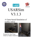
2.1.2 USARSim
Originally developed in 2002 at Carnegie Mellon University, USARSim (Unified
System for Automation and Robotics Simulation) [13] is a free simulator based on the
cross platform Unreal Engine 2.0. It was handed over to the National Institute of
Standards and Technology (NIST) in 2005 and was released under the GPL license [14].
USARSim is actually a set of add-ons to the Unreal Engine, so users must own a copy of
this software to be able to use the simulator. A license for the game engine usually costs
around $40 US [15]. Physics are simulated using the Karma physics engine which is
built into the Unreal engine [16]. This provides basic physics simulations [1]. One
strength of using the Unreal engine is the built in networking capability. Because of this,
robots can be controlled by any language supporting TCP sockets [17].
While USARSim is based on a cross platform engine, the user manual only fully
explains how to install it on a Windows or Linux machine. A Mac OS installation
procedure is not described. The installation requires Unreal Tournament 2004 (UT2004)
as well as a patch. After this base is installed, USARSim components can be installed.
8
On both Windows and Linux platforms, the installation is rather complicated and requires
many files and directories to be moved or deleted by hand. The USARSim wiki has
installation instructions [18]. Linux instructions were found on the USARSim forum at
sourceforge.net [19]. Since it is an add-on to the Unreal tournament package, the overall
size of the installation is rather large, especially on Windows machines.
USARSim comes with several detailed models of robots available for use in
simulations [20], however it is possible to create custom robot components in external 3D
modeling software and specify physical attributes of the components once they are loaded
into the simulator [21]. An incomplete tutorial on how to create and import a model
from 3D Studio Max is included in the source download. Once robots are created and
loaded, they can be programmed using TCP sockets [22]. Several simulation
environments are also available. Environments can be created or modified by using tools
that are part of the Unreal Engine [21].
There have been a multitude of studies designing methods for validating the
physics and sensor simulations of USARSim. Pepper et al. [23] identified methods that
would help bring the physics simulations closer to real-world robotic platforms by
creating multiple test environments in the simulator as well as in the lab and testing real
robotic platforms against the simulations. The physics of the simulations were then
modified and tested again and again until more accurate simulations resulted. Balaguer
and Carpin built on the previous work of validating simulated components by testing
virtual sensors against real-world sensors. A method for creating and testing a virtual
GPS (Global Positioning System) sensor that much more closely simulates a real GPS
sensor was created [24]. Wireless inter-robot communication and vision systems have
9
been designed and validated as well [20]. USARSim has even been validated to simulate
aspects of other worlds. Birk et al. used USARSim with algorithms already shown to
work in the real world as well as real-world data from Mars exploration missions to
validate a robot simulation of another planet [25].
2.1.3 SARGE
Figure 2.1.3 SARGE screen shot
SARGE (Search and Rescue Game Engine) [26], shown in Figure 2.1.3, is a
simulator designed to train law enforcement in using robotics in search and rescue
operations [27]. It is released under the Apache License V2.0. A screen shot can be seen
in Fig.1. The developers of SARGE provided evidence that a valid robotics simulator
could be written entirely in a game engine [1]. Unity was chosen as the game engine
10
because it was less buggy than the Unreal engine and it provided a better option for
physics simulations, PhysX. PhysX provides a higher level of fidelity in physics
simulations [11]. SARGE currently only supports Windows and Mac platforms though it
is still under active development. Currently, a webplayer version of the simulator is
available on the website http://www.sargegames.com.
It is possible for SARGE users to create their own robots and terrains with the use
of external 3D modeling software. Sensors are limited to LIDAR (Light Detection and
Ranging), 3D camera, compass, GPS, odometer, inertial measuring unit (IMU), and
standard camera [27], though only the GPS, LIDAR, compass and IMU are discussed in
the user manual [28]. The GPS system requires an initial offset of the simulated terrain
provided by Google Earth. The terrains themselves can be generated in the Unity
development environment by manually placing 3D models of buildings and other
structures on images of real terrain from Google Earth [28]. Once a point in the virtual
terrain is referenced to a GPS coordinate from Google Earth, the GPS sensor can be used
[11]. This shows that while terrains and robots can be created in SARGE itself, external
programs may be needed to set up a full simulation.
2.1.4 ROS
ROS [29] (Robot Operating System) is currently one of the most popular robotics
toolkits systems. Only UNIX-based platforms are officially supported (including Mac
OS X) [30] but the company Robotics Equipment Corporation has ported it to Windows
[31]. ROS is fully open source and uses the BSD license [32]. This allows users to take
part in the development of the system, which is why it has gained wide use. In its
meteoric rise in popularity over the last three years it has added over 1643 packages and
11
52 code repositories since it was released [33].
One of the strengths of ROS is that it plays nicely with other robotics simulators
and middleware. It has been successfully used with Player, YARP, Orcos, URBI,
OpenRAVE, and IPC [34]. Another strength of ROS is that it can incorporate many
commonly used libraries for specific tasks instead of having to have its own custom
libraries [32]. For instance, the ability to easily incorporate OpenCV has helped make
ROS a better option than some other tools. Many libraries from the Player project are
also being used in certain aspects of ROS [4]. An additional example of ROS working
well with other frameworks is the use of the Gazebo simulator.
ROS is designed to be a partially real-time system. This is due to the fact that the
robotics platforms it is designed to be used with, like the PR2, will be in different
situations involving more human computer interaction in real time than many current
commercial research robotics platforms [4]. One of the main platforms used for the
development of ROS is the PR2 robot from Willow Garage. The aim of using ROS’s
real-time framework with this robot is to help guide safe Human-Robot Interaction
(HRI). Previous frameworks such as Player were rarely designed with this aspect in
mind.
2.1.5 UberSim
UberSim [35] is an open source (under GPL license) simulator based on the ODE
physics engine and uses OpenGL for screen graphics [36]. It was created in 2000 at
Carnegie Mellon University specifically with a focus on small robots in a robot soccer
simulation. The early focus of the simulator was the CMDragons RoboCup teams;
however the ultimate goal was to develop a simulator for many types and sizes of
12
robotics platforms [37]. Since 2007, it no longer seems to be under active development.
2.1.6 EyeSim
EyeSim [38] began as a two-dimensional simulator for the EyeBot robotics
platform in 2002 [39]. The EyeBot platform uses RoBIOS (Robot BIOS) library of
functions. These functions are simulated in the EyeSim simulator. Test environments
could be created easily by loading text files with one of two formats, either Wall format
or Maze format. Wall format simply uses four values to represent the starting and
stopping point of a wall in X,Y coordinates (i.e. x1 y1 x2 y2). Maze format is a
format in which a maze is literally drawn in a text file by using the pipe and underscore
(i.e. | and _ ) as well as other characters [39].
In 2002, the EyeSim simulator had graduated to a 3D simulator that uses OpenGL
for rendering and loads OpenInventor files for robot models. The GUI (Graphical User
Interface) was written using FLTK [40]. Test environments were still described by a set
of two dimensional points as they have no width and have equal heights [41].
Simulating the EyeBot is the extent of this project. While different 3D models of
robots can be imported, and different drive-types (such as omni-directional wheels and
Ackermann steering) can be selected, the controller will always be based on the EyeBot
controller and use RoBIOS libraries [40]. This means simulated robots will always be
coded in C code. The dynamics simulation is very simple and does not use a physics
engine. Only basic rigid body calculations are used [41].
2.1.7 SubSim
SubSim [42] is a simulator for Autonomous Underwater Vehicles (AUVs)
developed using the EyeBot controller. It was developed in 2004 for the University of
13
Western Australia in Perth[43]. SubSim uses the Newton Dynamics physics engine as
well as Physics Abstraction Layer (PAL) to calculate the physics of being underwater [1].
Models of different robotic vehicles are can be imported from Milkshape3D files
[43]. Programming of the robot is done by using either C or C++ for lower-level
programming, or a language plug-ins. Currently the only language plug-in is the EyeBot
plug-in. More plug-ins are planned but have yet to materialize [43].
2.1.8 OpenRAVE
OpenRAVE [44] (Open Robotics and Animation Virtual Environment) is an open
source (LGPL) software architecture developed at Carnegie Mellon University [45]. It is
mainly used for planning and simulations of grasping and grasper manipulations as well
as humanoid robots. It is used to provide planning and simulation capabilities to other
robotics frameworks such as Player and ROS [46]. Support for OpenRAVE was an early
objective for the ROS team due to its planning capabilities and openness of code [46].
One advantage to using OpenRAVE is its plug-in system. Basically everything
connects to OpenRAVE by plug-ins, whether it is a controller, a planner, external
simulation engines and even actual robotic hardware. The plug-ins are loaded
dynamically. Several scripting languages are supported such as Pythos and
MATLAB/Octave [47].
2.1.9 RT Middleware
RT Middleware [48] is set of a standards used to describe a robotics framework.
The implementation of these standards is OpenRTM-aist, which is similar to ROS. This
is released under the Eclipse Public License (EPL) [49]. Currently it is available for
Linux and Windows machines and can be programmed using C++, Python and Java [48].
14
The first version of OpenRTM-aist (version 0.2) was released in 2005 and since then its
popularity has grown. Version 1.0 of the framework was released in 2010.
OpenRTM-aist is popular in Japan, where a lot of research related to robotics
takes place. While it does not provide a simulator of its own, work has been done to
allow compatibility with parts of the Player project [50].
2.1.10 MRPT
The Mobile Robot Programming Toolkit (MRPT) [51] project is a set of cross
platform C++ libraries and applications released under the GPL license. It is cross
platform, but has only currently has only been tested on Windows and Linux [52].
MRPT is not a simulator or framework; rather it is a toolkit that provides libraries and
applications that can allow multiple third-party libraries to work together [53]. The main
focus of MRPT is Simultaneous Localization and Mapping (SLAM), computer vision,
and motion planning algorithms [53].
2.1.11 lpzrobots
lpzrobots [54] is a GPL licensed package of robotics simulation tools available
for Linux and Mac OS. The main simulator of this project that corresponds with others
in this survey is ode_robots which is a 3D simulator that used the ODE and OSG
(OpenScreenGraph) engines.
15
2.1.12 SimRobot
Figure 2.1.12 SimRobot screen shot
Figure 2.1.12 shows a screen shot of SimRobot [55] is a free, open source
completely cross-platform robotics simulator started in 1994. It uses the ODE for physics
simulations and OpenGL for graphics [56]. It is mainly used for RoboCup simulations,
but it is not limited to this purpose.
A simple and intuitive drag and drop interface allows custom items to be added to
scenes. Custom robots can be created and added as well [57]. Unlike many of the other
robotics simulators, SimRobot is not designed around client/server interaction. This
allows simulations to be paused or stepped through which is a great help to debugging
16
simulations [57].
SimRobot does not simulate specific sensors as many of the other simulators do;
rather it only provides generic sensors that users can customize. These include a camera,
distance senor (not specific on a type), a “bumper” for simulating a touch sensor, and
“actuator state” which returns angles of joints and velocities of motors [57].
Laue and Rofer admit that there is a “reality gap” in which simulations differ from
real-world situations [56]. They note that code developed in the simulator may not
translate to real robots due to distortion and noise in the real-world sensors. They also
note, however, that code that works in the real world may completely fail when entered
into the simulation because it may rely on that distortion and noise. This was specifically
noted with the camera sensor and they suggested several methods to compensate for this
difference. [56]
2.1.13 Moby
Moby [58] is an open source (GPL 2.0 license) rigid body simulation library
written in C++. It supports Linux and Mac OS X only. There is little documentation for
this simulation library.
2.2 Commercial Robotics Simulators
There are many commercial robotics simulators available. Many of them are
designed for industrial robotics or a manufacturer’s own robotic platforms. The
commercial simulators described and compared in this paper will be focused on research
and education.
As with any commercial application, one downfall of all of these applications is
that they are not open source. Commercial programs that do not release source code can
17
tie the hands of the researcher, forcing them in some cases to choose the less than optimal
answer to various research questions. When problems occur with proprietary software,
there is no way for the researcher to fix it. This problem alone was actually the impetus
for the Player Project [4].
2.2.1 Microsoft Robotics Developer Studio
Figure 2.2.1 Microsoft Robotics Developer Studio screen shot
Microsoft Robotics Developer Studio (MRDS) [59] uses Phys X physics engine
which is one of the highest fidelity physics engines available [1]. A screen shot can be
seen in Figure 2.2.1. MRDS robots can be programmed in .NET languages as well as
others. The majority of tutorials available online mention the use of C# as well as a
18
Visual Programming Language (VPL) Microsoft developed. Programs written in VPL
can be converted into C# [60]. The graphics are high fidelity. There is a good variety of
robotics platforms as well as sensors to choose from.
Being a Microsoft product, it is certainly not cross platform. Only Windows XP,
Windows Vista, and Windows 7 are supported. MRDS can, however, be used to program
robotic platforms which may run other operating systems by the use of serial or wireless
communication (Bluetooth, WiFi, or RF Modem) with the robot [61].
2.2.2 Marilou
Figure 2.2.2 anykode Marilou screen shot
Figure 2.2.2 shows a screen shot of Marilou by anyKode [62]. Marilou is a full
robotics simulation suite. It includes a built in modeler program so users can build their
19
own robots using basic shapes. The modeler has an intuitive CAD-like interface. The
physics engine simulates rigid bodies, joints, and terrains. It includes several types of
available geometries [63]. Sensors used on robots are customizable, allowing for
specific aspects of a particular physical sensor to be modeled and simulated. Devices can
be modified using a simple wizard interface.
Robots can be programmed in many languages from Windows and Linux
machines, but the editor and simulator are Windows only. Marilou offers programming
wizards that help set up projects settings and source code for based on which language
and compiler is selected by the user [64].
Marilou is not open source or free. While there is a free home version, it is meant
for hobbyists with no intention of commercialization. The results and other associated
information are not compatible with the professional or educational versions. Prices for
these versions range from $360 to $2,663 [65].
20
2.2.3 Webots
Figure 2.2.3 Webots screen shot
The Cyberbotics simulator Webots [66] (shown in Figure 2.2.3) is a true
multiplatform 3D robotics simulator that is one of the most developed of all the
simulators surveyed [67]. Webots was originally developed as an open source project
called Khepera Simulator as it initially only simulated the Khepera robot platform. The
name of the project changed to Webots in 1998 [68]. Its capabilities have since expanded
to include more than 15 different robotics platforms [69].
Webots uses the Open Dynamics Engine (ODE) physics engine and, contrary to
the criticisms of Zaratti, Fratarcangeli, and Iocchi [22], Webots has realistic rendering of
both robots and environments. It also allows multiple robots to run at once. Webots can
21
execute controls written in C/C++, Java, URBI, Python, ROS, and MATLAB languages
[69]. This simulator also allows the creation of custom robotics platforms; allowing the
user to completely design a new vehicle, choose sensors, place sensors where they wish,
and simulate code on the vehicle.
Webots has a demonstration example showing many of the different robotics
systems it can simulate, including an amphibious multi-jointed robot, the Mars Sojourner
rover, robotic soccer teams, humanoids, multiple robotic arms on an assembly line, a
robotic blimp, and several others. The physics and graphics are very impressive and the
software is easy to use.
Webots has a free demonstration version available (with the ability to save world
files crippled) for all platforms, and even has a free 30 day trial of the professional
version. The price for a full version ranges from $320 to $4312 [70].
22
2.2.4 robotSim Pro/ robotBuilder
Figure 2.2.4 robotSim Pro screen shot
robotBuilder [71] is a software package from Cogmation Robotics that allows
users to configure robots models and sensors. A screen shot can be seen in Figure 2.2.4
Users import the models of the robots, import and position available sensors onto the
robots, and link these sensors to the robot's controller. Users can create and build new
robot models piece by piece or robotBuilder can import robot models created in other 3D
CAD (Computer-Aided Design) programs such as the free version of Google Sketchup.
The process involves exporting the Sketchup file as a COLLADA or 3DS file, then
importing this into robotBuilder [72].
robotSim Pro is an advanced 3D robotics simulator that uses a physics engine to
23
simulate forces and collisions [73]. Since this software is commercial and closed source,
the actual physics engine used could not be determined. RobotSim allows multiple
robots to simulate at one time. Of all of the simulators in this survey, robotSim has some
of the most realistic graphics. The physics of all objects within a simulation environment
can be modified to make them simulate more realistically [73]. Test environments can be
easily created in robotSim by simply choosing objects to be placed in the simulation
world, and manipulating their positions with the computer mouse. Robot models created
in the robotBuilder program can be loaded into the test environments. Robots can be
controlled by one of three methods; the Cogmation C++ API, LabVIEW, or any socketed
programming language [71].
robotSim is available for $499 or as a bundle with robotBuilder for $750.
Cogmation offers a 90-day free trial as well as a discounted academic license.
2.3 Conclusion
While this is certainly not an exhaustive list of robotics simulators, this is a simple
comparison of several of the leading simulator packages available today. Table A
contains a comparison table of the surveyed simulators and their relative advantages and
disadvantages. Items in the “disadvantages” column can be considered “show stoppers”
for many users.
Most of the simulators in this survey are designed for specific robotics platforms
and sensors which are quite expensive and not very useful for simpler, cheaper systems.
The costs and complexities of these systems often prevent them from being an option for
projects with smaller budgets. The code developed in many of these simulators requires
expensive hardware when porting to real robotics systems. The middleware that is
24
required to run on actual hardware is often too taxing for smaller, cheaper systems. There
simply isn't a very good 3D robotics simulator for custom robotic systems designed on a
tight budget. Many times a user only needs to simulate simple sensor interactions, such
as simple analog sensors, with high fidelity. In these cases, there is no need for such
processor intensive, high abstraction simulators.
CHAPTER 3: CONCEPT REQUIREMENTS
3.1 Overview of Concept
The concept of this simulator was conceived as a free (completely open source)
and cross platform 3D graphically and physically accurate robotics simulator. The
simulator should be able to import 3D, user-created vehicle models and real-world terrain
data. The simulator should be easy to setup and use on any system. It should also be
easy to allow others to develop in the open source community. The simulator should be
flexible for the user and be easy to use for both the novice and the expert.
3.2 Models of Robotic Vehicles
The models of robotic vehicles should be imported into the simulator in Ogre
mesh format. This format is one of several standard formats used in the gaming
community. These models can be created using one of many 3D modeling CAD software
programs. Several of these programs are compared in Appendix B.
3.3 Models of Terrain
Terrain models can be created by many means, however, in this project, terrains
are created only using Google Earth and Google Sketchup. Google Earth allows for a
seamless transfer of a given 3D terrain directly into Google Sketchup. Only the altitude
data is represented so there are no trees or other obstacles. This model could be used as
the basis for a fully simulated terrain.
26
3.4 Project Settings Window
Settings for the overall SEAR project should be entered in the Project Settings
Window. This records which models will be used for terrain, robot body and robot
wheels. The robot vehicle dynamics should also be set in this window to allow user
described values to be used in the physics simulations. User code files should be selected
in this window as well. The user has the option of selecting a custom user code file,
creating a new user code file template or creating a new Java file template in their chosen
working directory. All of the Project settings can be saved to a file, or loaded from a file
to ease set up of multiple simulations.
3.5 Sensor Wizard
The sensor wizard should allow users to enter important values for their sensors.
These values would then be stored to an XML file which will be read by the simulator
and used to set up sensor simulations.
3.6 User Code
A robotics simulator is of no use unless the user can test custom code. There are
two methods for users to create custom code. The user can use a template for a “User
Code File” which helps simplify the coding process of coding by allowing only three
methods to be used; a method in which users can declare variables, an initialization
method and a main loop method. This was designed to reduce confusion for novice users
and makes prototyping a quick and easy process. Additionally, the user could choose to
code from a direct Java template of the simulator itself. This would be a preferred
method for more advanced simulations.
27
3.7 Actual Simulation
Upon starting a simulation, the values recoded in the project settings file (.prj)
created in the Project Settings Window, the sensor settings XML file, and the user code
file (.ucf) should all be used to create the simulation. The paths to the models and vehicle
dynamics must then read from the project settings file. The simulator code itself is
modified by having the user code file integrated into it.
Once everything has been loaded, the simulator will begin. A graphical window
should open to show the results of a live simulation. The robot should drive around the
terrain interacting with the world either manually or using code written by the user.
Values of sensors should also be printed to the screen so the user can watch and debug
any problems. Once the simulation has finished, the user can close the simulator window
and edit the user code file again if needed for another simulation. Figure 3.7 shows the
basic work flow diagram of the entire project.
Figure 3.7 Basic work flow diagram of SEAR project
CHAPTER 4: TOOLS USED
This project relied on several software tools for development. The required
software ranged from code IDEs to 3D modeling CAD software. Netbeans 6.8 and 6.9
were used for coding Java for the project. The game engines used were jMonkeyEngine2
(jME2) and jMonkeyEngine3 (jME3). A variety of modeling software was used as well.
4.1 Language Selection
Using a previous survey of current robotics simulators [1] it was shown that
several of the current systems claim to be cross platform. While this may technically be
true, it is often so complicated to implement these systems on different platforms that
most people would rather switch platforms than spend the time and effort trying to set the
simulators up on their native systems. Most of the currently available open source
simulator projects are based on C and C++. While many of them are considered also
cross-platform, it takes a lot of work to get them running correctly for development on
different systems.
To make a simulator easy to use as well as easy to allow further development,
Java was selected as the language the simulator would be coded in. The development
platform used was NetBeans 6.8 and 6.9. This makes it very easy to modify the code,
and with the use of Java, the code can run on any machine.
4.2 Game Engine Concepts
The jME3 game engine consists of two major parts, each with their own "spaces"
29
that must be considered for any simulation. There is a "world space" which is controlled
by the rendering engine and displays all of the screen graphics. jMonkeyEngine does this
job in this project.
The second part is the physics engine which can simulate rigid body dynamics as
well as many other things. For this project only rigid body dynamics are being used,
however other systems can also be simulated such as fluid dynamics. The physics engine
calculates interactions between objects in the "physics space" such as collisions. It can
simulate mass and gravity as well.
A developer must learn to think about about both spaces concurrently. It is
possible for objects to exist in only one of these spaces which can lean to simulation
errors. Once an object is made in the world space, it must be attached to a model in the
physics space in order to react with the other objects in the physics space.
For instance, an obstacle created in only the graphics world will show up on the
screen during a simulation, however, the robot can drive directly through the obstacle
without being affected by it. Conversely, the obstacle can exist only in the physics world.
A robot in this instance would bounce off of an invisible object in a simulation. Another
option would be to have an obstacle created in both, but not in the same place. This
would lead to the robot driving though the visible obstacle, and running into its invisible
physics model a few meters behind the obstacle. Attention must be paid to attach both
the graphics and physics objects, and to do so correctly.
The game engine creates a 3D space or "world". In each direction, X, Y and Z the
units are marked as "world units." World units don't equate to any real-world
measurement. In fact they are set by the modeling tool used in model creation.
30
Experimentation with the supported shapes in the game engine shows that a one worldunit cube is very close to a one meter cube model. Certain model exporters will have a
scale factor; however that can be used to change the units of the model upon export.
Additionally, any object can also be scaled inside the game engine.
4.3 jMonkeyEngine Game Engine
The game engine selected for this project was jMonkeyEngine3 (jME3) since it is
a high performance, completely cross platform Java game engine. At the beginning of
this project, jME version 2.0 was used but development quickly moved to the pre-alpha
release of jME3 due to more advanced graphics and the implementation of physics within
the engine itself. The basic template for a simple game in jME3 is shown below:
public class BasicGame extends SimpleBulletApplication { public static void main(String[] args){ //create an instance of this class BasicGame app = new BasicGame(); app.start();//Start the game } @Override public void simpleInitApp() { //Initialization of all objects required for the game. //This generally loads models and sets up floors. } @Override public void simpleUpdate(float tpf) { //Main Event Loop } //end of Class
The superclass SimpleBulletApplication handles all of the graphics and physics
involved. Because this class is extended, local overrides must be included. The
31
simpleInitApp method is used to initialize the world and the objects within it.
The simpleInitApp method calls methods for loading models of the robotic
vehicle, loading the terrain models, setting up groups of collision objects, and any other
tasks that must be performed before the main event loop begins. simpleInitApp then sets
up all the internal state variables of the game and loads the screengraph [74]. The
simpleUpdate method is the main event loop. This method is an infinite loop and is
executed as fast as possible. This is where important functions of the simulator reside.
The actual simulation of each sensor and updates to the simulator state are done in this
loop. Additionally, other methods from the simpleBulletApplication may be overridden
such as onPreUpdate and onPostUpdate, though these were not used specifically in this
project.
4.4 Jbullet-jME
The JBullet physics engine was chosen for this project. JBullet is a 100% Java
port of the Bullet Physics Library which is originally written in C++. During early
development of this project using jME2, the development of a JBullet implementation for
jME2 (called JBullet-jME) was used. Jbullet-jME development was stopped after only a
few weeks of development so a completely new implementation of JBullet could be
integrated in the new version of jMonkeyEngine, jME3.
The concept was to combine the graphics and physics engines to result in a
complete game engine. This game engine was also coupled with a newly developed
modification of the Netbeans IDE (Integrated Development Environment) to be released
as jMonkeyPlatform. This triad of development tools was not complete when this thesis
project began and therefore was not fully utilized. Additional problems with speed and
32
compatibility made the use of the pre-Alpha version of the jMonkeyPlatform very
unreliable and it was not used for this project.
4.5 Overview of Previous Work
At a thesis topic approval meeting, A 3D model of a robot from the Embedded
Systems lab was constructed in Google Sketchup. The model was then exported as a
COLLADA file and loaded into a jME2 application using JBullet-jme. A real-world 3D
terrain exported from Google Earth to Google Sketchup and a third-party free plug-in
was used to generate a height-map JPEG image which was also loaded into the jME2
program. The robot was driven around the scene showing the reactions to collisions as
well as the effects of gravity and velocity on the objects in the scene.
More development using jME2 and Jbullet-jme was not possible since not many
functions were released for the JBullet-jme engine. Development of the simulator had to
switch to the new pre-Alpha jME3 platform onto which all jMonkey development focus
had been switched. The jME3 engine integrated the JBullet physics engine into the game
engine. Because of this fact, any code using it had to start from scratch. This lead to
several systems not being implemented at the time this project switched game engines.
For instance, the terrain system as well as model loading had not yet been written for
jME3 when the project switched game engines. In fact, COLLADA models were no
longer planned to be natively supported. Everything written in jME2 was now also
deprecated code and practically nothing would convert to the new engine. All previous
code for the robotics simulator had to be scrapped.
Throughout this project, nightly builds of the pre-Alpha version of jME3 were
downloaded from the jMonkeyEngine code repository to get the newly support
33
functionality. The use of these nightly builds lead to many code rewrites and much of the
time spent was for waiting for certain features to be implemented in jME3. During these
times work on other concepts was accomplished, such as methods for simulating sensors,
logical layout of the program, graphical user interface (GUI) design and research on other
simulators. The graphics capabilities of jME3 were much more advanced, and as such
would only now on machines that supported OpenGL2 or above [75]. This reduced the
available machines that could be used for development to one. Because of all of these
factors, several months passed before the jME3 version could match the capabilities of
the original jME2 project.
CHAPTER 5: IMPLEMENTATION
5.1 General Implementation and Methods
Since this project began during early pre-alpha stages of jME3, functionality for
many features of the program were delayed and in several cases had to be completely
redeveloped after updates to the engine rendered code deprecated. Therefore, this project
evolved and changed as functionality was added to jME3.
5.1.1 Models of Robotic Vehicles
Loading a robot vehicle model is done as a call to the RobotModelLoader class in
the ModelLoader package of the Netbeans project. This code was written by Arthur
Carroll in the early stages of this project to serve as an easy method for building robots
from the separate models of the robot body, and all four wheels and its listing can be
found in Section F.1. This process is invisible to the user as it happens directly in the
Simulator.java file. The user only has to select the location of the models of the robot
body, and each wheel in the Project Settings Window. Additionally, the user has fine
grain controls to change the position of each of the wheels. Future versions of this code
will load an entire robot model from a .scene file.
5.1.2 Models of Terrain
The user has only to select the location of the model they want to load in the
Project Settings window when setting up a project. The terrain loading process is carried
out in the Simulator.java file and involves calling the TerrainModelLoader class (Section
35
F.2) in the ModelLoader package of the Netbeans project. This serves as a simple
method of importing and creating a terrain from an Ogre mesh model.
5.1.3 Obstacles
Obstacles are added to the test environment using built-in methods. These
methods are called by the user in the initialization function of the user's code. Currently,
the only two supported obstacles are a one-meter cube and a tree. To add a tree to the
environment, the user can simply pass a 3D location to the addTree() method (e.g.
addTree( x, y, z ); where z, y, and z are in world units.) The addBox() method works
similarly. Using the boxes as bricks, the user can build different structures. By adjusting
the mass of the boxes (by editing the addBox() method directly) the user can create solid
walls that will not crumble or break when hit by a vehicle. Future development will yield
an addWall() method that will allow users to build walls of a building or maze quickly
instead of building them out of many boxes.
5.1.4 Project Settings Window
The SEAR Project Settings window is the first jFrame window the user will see.
It is from this window that the user will set up a simulation project. The user must select
which models will be used for the terrain, the robot body, and each of the robot wheels as
well as setting initial locations of all of these models. Additionally the dynamics of the
robotic vehicle can also be set, such as mass, acceleration force, brake force, suspension
stiffness, suspension compression value, and suspension damping value. Default
workable values are set so the user may have a starting point for their vehicles. The user
must also select the directories in which the jMonkey .jar libraries reside as well as their
own user code file. Additionally, the user can select to activate the debug shapes in the
36
simulator. This option visibly shows a representation of the physics shapes used in the
simulation and can be vital for debugging simulation results. The Sensor Wizard
(discussed in detail in Section 5.1.5) may also be called from the Project Settings
window.
The “Terrain Mode” tab shown in Figure C.1 Allows the user to select the
location of the terrain model and set the latitude, longitude and altitude values of the
center of the terrain. Figure C.2 shows the “Robot Body Model” tab which allows the
user to select the location of the model of the robot body. This tab also has options to set
the model's position and rotation within the terrain. These options should be used as
course grain measurements as the robot will likely roll if the terrain is slanted anyway.
The “Wheel Models” tab shown in Figure C.3 has options to select the location of each
wheel model as well as options for relative positioning of each of these models to the
main robot body. These settings are optional depending on the models as some models
already have the offsets designed into each of the models. Figure C.4 shows the vehicle
“Dynamics” tab which has several options for vehicle dynamics, such as vehicle mass,
acceleration force, brake force, and suspension configurations such as stiffness,
compression and damping values. The fields are filled in with default values for a
workable robot vehicle. Other options are planned for this tab such as lowering the
center of gravity of vehicle and the amount of friction slip of each wheel. If values are
changed by the user, the “Reset Defaults” button will reset the default dynamics values in
this tab. The “Code Setup” tab shown in Figure C.5 allows the user to create blank user
code file and simulator.java templates, select the location of the preinstalled jMonkey .jar
libraries, and select whether or not the simulator will run in debug mode. Debug mode
37
shows all of the physics shapes in the world to allow for debugging of model physics.
The "Simulate", "Sensor Wizard", "Save Project" and "Load Project" buttons are
located at the bottom of every window, in the main jFrame. The “Sensor Wizard” button
launches the Sensor Wizard GUI. Save Project will allow the user to save all of the
settings for the current project as a “.prj” project file. Currently, the file is saved as a
simple text file in which each line corresponds to a setting in the Project Settings window,
however future plans call for this file to be written in XML. The “Load Project” button
allows the user to select a previously saved project settings file so the user won't have to
enter them each time the simulator is run. The Simulate button allows the user to
simulate the project in the simulator. Before each simulation begins, all of the settings
for a project must be saved. This is due to the fact that the simulator itself is compiled
dynamically, but called as a separate system process. The simulator must open and read
the project settings file to initialize variables for the simulation. A more detailed
explanation of the processes that occur when the Simulate button is pressed is located in
Section 5.1.7 of this thesis. The code listing for the Project Settings Window can be
found in Section F.3 of this thesis. The dynamic compiler listing can be found in Section
F.4.
5.1.5 Sensor Wizard
The Sensor Wizard (code listing available in Section F.5) is designed to provide a
simple way for a user to enter information about each sensor and consists of a jFrame
similar to the Project Settings window which allows the user to specify values and
information about each of the sensors. The options for each sensor are saved as sensor
objects which are then written out to an XML file. The “Infrared (IR)” tab (Figure D.1)
38
shows the options available for setting up the properties of the IR beam including beam
width, maximum and minimum distance. These values are only available for analog
sensors. If the “Digital Output” radio button is selected, the only options available
describing the beam are beam width and switching distance. Figure D.2 shows the
“Ultrasonic” sensor tab. This tab has many of the same options as the Infrared tab, but
there is no option for digital or analog sensor selection. Both the “Infrared (IR)” and
“Ultrasonic” tabs will have a an additional field in which sensor resolution is set. These
values, including resolution, will be used in the method described in Section 5.2.2.1 for
simulating distance sensors. The “GPS” sensor tab is shown in Figure D.3 and has
options for String Type which specifies the output string from the GPS unit. “Update
Speed”, “Accuracy” and” Bandwidth” are the other options available for this sensor type.
Figure D.4 shows the “LIDAR” settings tab. Options available to the user are angle
between readings in degrees, maximum sensing distance, and resolution. The
“Accelerometer” and “Gyroscope” tabs are shown in Figures D.5 and D.6. These two are
described together and most of their options are similar. There are options for selecting
the relevant axis, resolution, accuracy, bandwidth and maximum range. For the
accelerometer, the units of resolution are in millivolts per G and maximum range is in Gforces. For the “Gyroscope” tab, the units of resolution and maximum range are in
degrees per second. Figure D.7 shows the options in the “Compass” tab. The option
fields currently listed in this tab are dummy options as the variety of magnetometers and
compass units don't all have the same options. Once a better options scheme is
determined, or a family of sensors are selected these fields will be changed. The
“Odometer” tab is shown in Figure D.8 and has dummy option fields in the current
39
design. Again, once a specific method of odometry is selected for simulation, the names
of these fields will be changed.
The options listed for each sensor can be found in the sensor's manufacturer
datasheet and user manual. For each sensor, there are options for “Sensor Name” and
Sensor Model” which will be used to create different sensor objects, allowing for
multiple copies of each sensor to be loaded. Once a sensor's options are set in its
perspective window, the add sensor button must be pressed to save those options. Once
all of the options for all sensors are set, clicking the “Save and Close” button serializes all
of the options for each sensor and writes them to an XML file.
This XML file is to be read by the sensor classes to set up a particular sensor's
relevant data. For instance, the accelerometer and gyroscopes require a bandwidth or
update frequency which is used in the simulation. Once these values are entered into the
sensor wizard, they are written to “Sensors.XML”. The Sensor Wizard has all of the
proposed supported sensor types that will be available in the future and is not currently
being used in the simulator. This is because the concept for the usage of the XML file
relies on 3D models of sensors attached to the robot vehicle model. This function will be
implemented in future additions of the simulator as it requires the integration of a .scene
model loader to load a complete robot vehicle model which has yet to be integrated into
the simulator.
All of the sensors are treated as Sensor objects (code listing can be found in
Section F.6 Sensor.java) based on the example by Thornton Rose [76]. Each of these
objects have a specific type (Section F.7 SensorType). Sensors are then split into two
subtypes, Location sensors (Section F.8 Location.java) sense the current location and
40
consist of GPS (Section F.9), Compass (Section F.10), Accelerometer (Section F.11),
Gyroscope (Section F.12) and Odometer (Section F.13) sensors. Distance sensors
(Section F.14) make up the second subtype and include Infrared ( Section F.15),
Ultrasonic (Section F.16) and LIDAR (Section F.17). When the “Add Sensor” button is
clicked on any of the tabs in the Sensor Wizard window, that sensor is added to a
SensorContainer ( Section F.18) which is then written out to an XML file. Currently a
prototype XML reader (readXML, Section F.19) will read in the XML file, create sensor
objects from the data within it, and print that data to a terminal along with a count of total
number of sensor objects detected.
5.1.6 User Code
A blank user code file template is copied to a directory of the users choice by
clicking “Create New UCF file” button in the Project Settings window “User Code” tab.
The path to this file should not contain any spaces to assure it is found during
compilation. The file is then edited in an external text editor and saved by the user.
Compilation of the user code can be handled two different ways. For simple
simulations, the User Code Template can be selected. The template is edited in any
standard text editor outside of the the simulator. The User Code Template consists of
three methods, userVariables(), init(), and the mainLoop(). Variables must be in the
userVariables() method. The addition of obstacles (using addTree() or makeBox()
methods) as well as information to set up sensors is done in the init() method. Code that
reads the sensors or controls the robot vehicle should be written into the mainLoop()
method. Upon clicking the “Simulate” button in the Project Settings window, the User
Code File is copied into a standard Simulator template file, and saved to the user's current
41
directory. The code inside the userVariables() method is copied into the Simulator class
as global variables. The code inside the init() method is copied into the initSimpleApp()
method of the Simulator file and the mainLoop() method is copied into the
simpleUpdate(); method. Below is an example of a blank User Code File. A listing of
the User Code File template can be found in Section F.20.
userVariables(){ /* Do NOT EDIT THIS LINE */ /**User Global Variables go here. **/ }; init(){ /* Do NOT EDIT THIS LINE */ /**User Initialization Code goes here. **/ }; mainLoop(){ /* Do NOT EDIT THIS LINE */ /** User Program Code goes here: */ }; If the user requires the use of custom methods that cannot be defined in the User
Code File template, they can manual edit the Simulator Java code template directly.
Section F.21 is a listing for the SimulatorTemplate.txt file.
Once the simulation begins, the vehicle may be driven around manually using the
keyboard to position it for the beginning of the simulation. The camera may also be
moved during this time. User code is executed only after the space bar has been pressed.
Once the simulation is started, the camera begins to follow the vehicle. A simulation may
be restarted by pressing the enter/return key. This resets the robot to the original position
in the world where it can again be controlled by the keyboard. Table 5.1.6 below shows
keys and their functions.
42
Table 5.1.6 Keyboard controls of the Simulator Window
Key
Action
H
Spin Vehicle Left
K
Spin Vehicle Right
U
Accelerate Vehicle
J
Brake Vehicle
Enter
Reset Robot Position
Space Bar
Begin User Code
Q
Pan Camera Up
W
Pan Camera Forward
A
Pan Camera Left
S
Pan Camera Backward
D
Pan Camera Right
Z
Pan Camera Down
43
5.1.7 The Simulation Window
Figure 5.1.7 Simulator window showing gyroscope, accelerometer, GPS and Compass
values as well as the robot vehicle model, and a tree obstacle. The terrain is from Google
Earth of the track at the University of North Carolina at Charlotte.
Once all of the settings for a particular simulation are set, the user clicks the
“Simulate” button in the Project Settings window. At this point, many things happen.
First, the project settings are saved to a file. Then the user coded file is merged with a
clean copy of a SimulatorTemplate text file. This happens in several steps. A blank text
file named “Simulator.java” is opened in the user's current working directory (the
directory in which the User Coded File resides). Then a clean copy of a
SimulatorTemplate.txt template provided by the simulator is opened and copied into the
blank text file until the line “/**User Variables Declared Below this Line */” ” is
44
encountered. At this point, the User Coded File is opened and the lines between
“userVariables(){ /* Do not edit this line */” and the ending curly bracket “};” are
copied into the newly opened file. Then the SimulatorTemplate.txt again is copied into
the blank text file until it reaches the line “/**User Initialization Code goes Below here.
**/”. It will then copy the code within the init() method from the User Code File into this
section until it reaches the ending curly bracket “};” of the init() method. Once again, the
SimulatorTemplate.txt continues to be copied into the blank text file until it reaches the
line “/** User Program code goes here: */”. It will then copy the code within the
mainLoop() method from the User Code File into this section until it reaches the ending
curly bracket “};” of the mainLoop() method. The remaining lines from the
SimulatorTemplate.txt file are written to the blank text file. Once all lines are written, the
files are closed. At this point, the User Code File has been fully integrated into the
Simulator's code. The resulting code (named Simulator.java located in the same directory
as the User Code File) is dynamically compiled.
If there were no errors during compilation, a process is spawned to run the
resulting Simulator.class file. (The resulting Simulator window is shown in Figure 5.1.7.)
The choice to run the simulator as a process rather than to dynamically load the class was
chosen for two reasons. The first being that it is very simple compared to writing a
custom classLoader, and the second being the fact that users will likely run multiple
simulations during one session. It is hard to write a dynamic classLoader that will fully
unload a class after it has run so a new version of that class could be loaded. Having the
class run as a process eliminates a lot of this code overhead.
Because the Simulator.class file is run as a process, this means that it is fully
45
separate from the Project Settings window and Sensor Wizard. Information about the
sensors is loaded from the Sensors.XML file, and information on how to load the models
is located in the project settings file (.prj). Since the user can save the project settings file
anywhere they choose, the path to this file is passed as an argument to the simulator when
it is called as a process.
Currently, the user can not use loops in the mainLoop() method due to the way the
game engine works. The code in the mainLoop() method is copied into the
simpleUpdate() method of the simulator, where all of the physics and graphics are
updated. Since loops controlling the robot vehicles rely on updates from this loop, the
programs will get stuck in an infinite loop, never breaking out or actually updating
because they are holding up the simpleUpdate(); loop. Therefore, all robot vehicle
controls and sensor value filters must be modeled as finite state machines. Future
editions of this software will use TCP/IP sockets for all sensors and robot vehicle
controls, thereby allowing loops and all other normal coding components and
conventions, eliminating the need for dynamic compilation of user code, and allowing
users to use many different programming languages.
5.2 Sensor Simulation
All sensors are simulated in the physics space. There is no real need for a
graphical representation of them at this point, however, as this simulator is developed
further it is expected that users can add and position 3D models of sensors to their robot
models completely graphically.
5.2.1 Position Related Sensor Simulation
Autonomous robotic vehicles rely very heavily on knowledge of their locations in
46
3D space. Without this information, autonomous control of the vehicle is impossible.
For this reason, the class of positional sensor simulators was created.
5.2.1.1
GPS
GPS simulation is not a new concept as shown by Balaguer and Carpin. [24].
Though Balaguer and Carpin describes and tests an advanced GPS simulation algorithm,
it is sufficient to simulate GPS with only basic functionality. To simplify GPS
simulations, satellite tracking is not required. Additionally, no attention has been paid to
simulating actual GPS inaccuracies due to atmospheric conditions or other causes. Basic
functionality of GPS is simulated to provide only the Latitude, Longitude and Altitude
measurements of the vehicle's current position. To further simplify the simulation, GPS
is simulated as a rough flat projection of the terrain. This is similar to the simple version
of the GarminGPS sensor in early Gazebo simulations [77] developments will improve or
replace this implementation, but it is important to have a simple and basic version of this
sensor for initial tests of the simulator.
There are several important settings that the user must enter before using the GPS
sensor in a simulation. The first set of values represents the latitude, longitude and
altitude values of the center point of the terrain map being used. These values are then
converted from a string to complete decimal format and will be used as an offset which
helps calculate the current latitude, longitude and altitude of the robotic vehicle during
simulation. Another set of values entered by the user indicate the location of the robotic
vehicle. Again, latitude, longitude and altitude are required. These values are used to
position the robot within the terrain at the start of the simulation. Finding values for the
latitude and longitude for both the terrain and the starting position of the vehicle are
47
easily obtained from the Google Earth before exporting the terrain map. Appendix E
goes into detail on exactly how to find these values.
Since the Earth is not a perfect sphere, the length of a longitude degree varies
from 111,320 meters per degree at 0 degrees latitude (the equator) to 0 meters per degree
at 90 degrees latitude (the poles) [78]. Calculating this value on a constant basis can
prove rather costly on computing resources. To simplify the changes in longitudinal
distances, a lookup table based on the Zerr's table is used to simulate distance per degree
latitude. The value entered by the user of the starting position of the robot vehicle will be
used in this lookup table to find the closes matching latitude.
Since it is impractical that a simulation will require a vehicle to travel more than
five latitudinal degrees, the value of the length of a degree is never recalculated during
the simulation.
To find the distance per degree longitude in this simulator, a simple distance
Formula (5.2.1.1.1), is used [79].
Length of a degree of Longitude
= Radius of Earth at the Equator×cos( Latitude)
(5.2.1.1.1)
Distance of a degree of longitude at the equator = 111320.3411 meters as shown
by Zerr. So the final formula is shown in Formula (5.2.1.1.2).
Length of one degree of Longitude
=111320.3411 meters×cos ( Latitude)
(5.2.1.1.1)
Since this formula is small and is a fast calculation it can be calculated each time
the GPS simulator is polled without a large determent to the speed of the overall
simulation.
When the GPS simulator is polled, it finds the distance in three dimensions of the
48
vehicle from the center of the world space from the current position of the vehicle .
These values are returned in world units and are treated as meters (in this simulator, one
world unit equals one meter). Knowing the offset in three dimensions in meters from the
center point of the map as well as the values of the center of the map, the latitude,
longitude and altitude of the vehicle can be calculated. The current vehicle position on
the X-axis in meters of the vehicle is converted to latitude using the values from Zerr's
table. The latitude of the vehicle is then known and can be used in Formula 5.2.1.2 to
find the length per degree longitude. The current vehicle position in the Z-axis (in
meters) is then divided by this value to find the current longitude of the vehicle. The
current vehicle offset in the Y-axis is added to the value of the altitude of the center of the
terrain map. This gives the actual vehicle altitude in relation to the original center value.
The code listing for the GPS sensor simulator can be found in Section F.22.
Table 5.2.1.1 GPS Simulator Attribute Table
Function
Datatype
Variable Name
Notes:
Input
boolean
GPSActive
In Simulator.java used to activate
GPS simulator
Input
boolean
degreeOutput
Input
Vector3f
WorldCenterGPS
Output
Vector3f
GPSResults
Located in GPSSimulator.java
Denotes output type.
True = Degree Format,
False = Decimal Format
Located in GPSSimulator.java
Sets the location of the center of
the terrain
Stores results of a GPS
calculation. Set equal to
simulate(physicsVehicleNode)
method
49
5.2.1.2
Compass
The compass simulator is single-axis and very simple. A Vector3f is used to store
the position of North. For example, North will be located at x, y, z ordinates (100000, 0,
0). Since one world unit equals one meter in this simulator, this means the magnetic
North Pole is 100km along the X-axis of any simulation. Of course, this value can be
changed by the user to a more accurate estimation of actual pole distance when the
latitude and longitude of the terrain are considered. For an accurate calculation, users can
visit the NOAA (National Oceanic and Atmospheric Administration)National
Geophysical Data Center magnetic declination calculator online to calculate the current
magnetic declination of any latitude and longitude and at any given time [80]. Users can
then calculate the appropriate current position of magnetic North, and enter this value, in
world units, as the simulator's North value.
The simulator calculates the angle of the robot to north by getting the values of
the forward direction of the robotic vehicle using the getForwardVector() method. The
values of this vector of the X and the Z directions represent the forward facing direction
in the X-Z plane. These values are compared to the X and Z values of "North.” The angle
between these two values is the angle between the forward-facing direction of the robotic
vehicle and North. This angle is represented in +/-180 degrees (or +/- PI radians).
The location of North in the Google Maps terrain corresponds to the X direction
when the terrain is exported correctly (with North facing upward). This automatically
sets North in the terrain model to the X direction in the simulator.
A future version of this sensor could integrate a closer model by calculating the
distance to magnetic North based on the Latitude and Longitude, though this measure
50
would only be valid for a few years as the Earth's pole moves constantly. The code listing
for the compass simulator can be found in Section F.23
Table 5.2.1.2 Compass Attribute Table
Function
Datatype
Variable Name
Notes:
Input
boolean
compassActive
In Simulator.java used to activate
Compass simulator
compassDegrees
Located in
CompassSimulator.java Denotes
output type.
True = Degree Output
False = Radians Output
north3f
Located in
CompassSimulator.java Sets the
location of North
Input
Input
boolean
Vector3f
Output
float
5.2.1.3
CompassResults
Stores results of a Compass
calculation. Set equal to
simulate(physicsVehicleNode)
method
Three-Axis Accelerometer
The use of MEMS (Microelectromechanical Systems) accelerometers are
becoming very common in the world of robotics in recent years. Accelerations can be
used in dead-reckoning systems, as well as force calculations.
Simulation of accelerations is made simpler because of several methods built into
jME3. jME3 provides a getLinearVelocity() method which will return the current linear
velocity of a physicsVehicleNode in all three dimensions. To get accelerations from this
method, a simple integration of these vales over time is taken. To get an accurate time
the timer class was used. The timer class provides two important methods used in this
integration, getResolution() and getTime(). getResolution() returns the number of “ticks”
per second and getTime() returns the time in “ticks”. These two values together are used
51
to find time in seconds.
The accelerometer has a bandwidth set by the user. This represents the frequency
at which the sensor can take measurements. The bandwidth is converted to time in
“ticks” by inverting the bandwidth and multiplying by the timer.getResolution() method.
The result is the number of ticks between two measurements of linear velocity. The
accelerometer method is called from the main event loop in the simulator Java code .
This allows it to function continuously during the simulation. Because of this fact,
however, the accelerometer simulator must not take too much time to execute, otherwise
it will slow down the entire simulation. To make sure the main event loop executes
quickly the accelerometer method does not stall for the given time between
measurements, rather it stores a starting time and calculates the time that has passed
every time the main event executed. The elapsed time is compared to the number of ticks
between readings calculated from the bandwidth.
On the first run of a single reading, the first linear velocity is returned from the
getLinearVelocity() method and saved, then the getTime() method saves the current time
(in “ticks”) and a flag is set to prevent this from happening again until the next reading.
Every time the main event loop runs, it calls the accelerometer method which now
compares the elapsed time from the first reading with the number of ticks between
readings calculated from the bandwidth. When this time has finally elapsed the second
linear velocity is taken and immediately an ending time is saved. The total number of
seconds passed between readings is found by subtracting the number of ticks that have
elapsed during the measurement, and dividing this difference by the resolution of the
timer from the getResoultion() method. The acceleration is equal to the second velocity
52
minus the first velocity divided by the elapsed time in seconds Formula 5.2.1.3. Once a
single reading is finished, the flag for reading the first velocity and starting time is reset.
Velocity 2−Velocity 1 
Elapsed Time in Seconds
(5.2.1.3)
These readings are for all three axes. The decision was made to return the
resulting values from all three axes every time the accelerometer is used. If a user is only
interested in one axis, the others can be ignored. The code listing for the accelerometer
simulator can be found in Section F.24.
Table 5.2.1.3 Accelerometer attribute table.
Function
Datatype
Variable Name
Notes:
Input
boolean
accelActive
In Simulator.java used to activate
Accelerometer simulator.
bandwidth
Located in AccelSimulator.java
Denotes the frequency of a
sensor update
accelValues
Stores results of a Accelerometer
calculation. Set equal to
simulate(physicsVehicleNode)
method.
Input
Output
float
Vector3f
5.2.1.4
Three-Axis Gyroscope
Gyroscopes often accompany accelerometers in the design of inertial measuring
systems. They can be used to help correct offsets and errors given by real-world
accelerometers. Since there is no error in the simulated accelerometers in this simulator,
there is no need for this, however users may still want to use them in this way to improve
filtering algorithms. Real-world MEMS gyroscopes often have a large output drift. This
isn't currently simulated, however future work will include a user-adjustable coefficient
of drift to improve the simulator.
53
jME3 has a method to return angular velocity, however, it does not return values
in radians per second. In fact, I could not determine exactly what units it returned even
with the help of the developer's forum. A custom method for finding actual angular
velocity was created that is very similar to the accelerometer simulator.
Again, jME's timer class was used to find timer resolution (in “ticks” per second)
and elapsed time, in ticks. To find the angle traveled over an elapsed time, the
getForwardVector() method was used. This method returns the 3D normal vector of the
forward direction of the PhysicsVehiceNode. The time between measurements was again
calculated from a user-defined bandwidth for the sensor. For the first run of a sensor
reading, the first forward direction vector and start time are recorded then a flag is set to
prevent this from happening again until the next reading. The current time is compared
with the expected elapsed time until it is reached. At this point the second forward
direction vector is recorded as well as the stop time. Since the Vector3f class has no
methods for comparing the angle between the components, both of the forward vectors
are projected on each of the three original planes; XY, YZ and XZ. Each of these values
are stored in a Vector2f. Using the angleBetween() method in the Vector2f class, the
angle between each projected portion of the forward directions are calculated. For
example, XY1 are the X and Y components of the first forward vector, XY2 are the X
and Y components of the second forward vector. XY1.angleBetween(XY2) returns the
angle between these components. This would describe a rotation about the Z-axis. Once
the angle traveled in each axis is found the elapsed time is used to find the angular
velocity. The angular velocity is then returned to the user in the format (either radians per
second or degrees per second) the user selected when setting up the sensor. As with the
54
accelerometer, all three axes are always simulated. The code listing for this sensor
simulator can be found in Section F.25.
Table 5.2.1.4 Gyroscope attribute table
Function
Datatype
Variable Name
Notes:
Input
boolean
gyroActive
In Simulator.java used to activate
Gyroscope simulator.
Input
float
bandwidth
Located in GyroSimulator.java
Denotes the frequency of a
sensor update
angularVelocity
Stores results of a Gyroscope
calculation. Set equal to
simulate(physicsVehicleNode)
method.
Output
Vector3f
5.2.1.5
Odometery
Odometry is a very useful metric used in positioning calculations for vehicles. An
odometer simulator is planned but has yet to be researched or studied in detail, though a
method for measuring odometric values may be inherent if the vehicle wheels are
replaced with jMonkey “hinge” or “joint” physics nodes as the rotation angles of these
pivot points are controlled directly. Regardless of the method of implementation, future
releases of this software will have an odometry sensor simulator.
5.2.2 Reflective Beam Simulation
Beam reflection sensors are arguably the most common sensors used in robotics.
This sensor class includes both Infrared (IR) and Ultrasonic sensors. Though the
technologies behind these two types of sensor differ, they operate on the same principles.
This type of sensor works by sending a signal out into the world, and measuring the time
it takes for that signal to reflect back to the sensor. These sensors come in both analog
55
and digital output varieties.
5.2.2.1
Infrared and Ultrasonic Reflective Sensors
With digital outputs, the senor has a binary output based on a set threshold. For
instance, the Sharp GP2D15J0000F returns a logic HIGH on its output when it detects
objects within a maximum distance of 24cm [81]. This type of sensor is fairly easy to
simulate using a broad-face approach. A model of the sensor's beam shape is loaded as a
ghostNode in the simulator. A ghostNode is a type of physicsNode available in jME3 that
will not affect the other objects in the physics world of the simulator, but can report all
collisions. Any time a collision is detected with this node, the simulated sensor returns a
positive result.
During testing of the ghostNode method for simple collisions, it was found that
the ghostNode implementation in jME3 returns spurious false collisions. Discussions
with the online developer's forum provided no help on this matter as it isn't a priority for
the development team yet. This sensor will be simulated the same as an analog sensor,
except with a distance threshold the user can set to simulate the switching distance of the
sensor.
Sensors that output analog values cannot be simulated using a broad-face method.
The only tool available in the physics engine that can simulate an analog measurement of
this type is a Ray. Rays are infinitely long lines that begin at an infinitesimally small
point and travel in a given direction. Collisions between rays and other objects can easily
be checked. The information about a collision is stored in a CollisionResults object. This
information consists of the name of the object hit, the object type, and the coordinates (in
World Units) of the collision in X, Y and Z dimensions. The nature of the ray allows it to
56
go through objects as well as collide with all objects in its path which can lead to multiple
collisions. If collisions exists, the closest collision can be found.
For a very simplistic simulation of an analog sensor, a single ray can be used.
These simulations can be very fast, however they are not very accurate to real-world
sensors. To more accurately simulate these sensors, the properties of the entire beam
shape of the sensor must be recreated casting a multitude of rays to form a set of nested
cones. IR and Ultrasonic beams can have a variety of different shapes depending on the
applications they are used for. IR beams for the Sharp family of IR sensors generally
have a roughly ovate or “football” shape while the MaxBotix EZ series ultrasonic sensors
have more of a teardrop shape [82] - [84] . A single 3D teardrop volume was selected to
simulate the best ranges of the IR beam as well as the ultrasonic beam.
To create the cone shape, several arrays of rays will be nested within one another.
Each array will create a single cone. As the radius decreases, the cones become longer
and thinner. The measuring length (or limit) of all the rays will be the same, thus creating
more of the teardrop shape. This concept was exaggerated and then simulated with
visible lines as shown in Figure 5.2.2.1 to clarify the explanation.
57
Figure 5.2.2.1 Visible simulation of beam concept. Each nested cone has a different color
to make it easier to see. The axis lines depict the Y-axis (pointing upward) and the Z-axis
(pointing right).
Each line in the figure above represents a single ray that is cast. The distance
between the rays in a cone is calculated by using the resolution of the senor which is
given by the user when setting up the sensor. The distance in the Y direction from one
cone to the next also uses this value. Therefore as the resolution distance increases, the
number of rays (and cones) decreases. The resolution of any sensor is often given in the
datasheet but if it is not, simple testing with dowels of differing diameters may be used
for rough estimates [83]. A one inch diameter pipe can be used to give a rough estimate
of the sensing distance of a sensor [85]. The closest collisions of each ray is compared,
returning the closest overall collision in world units.
58
The position of each ray is calculated by creating a starting point for the outermost
cone. The position of the first ray is calculated using information about the beam shape
provided by the user. At this point, the ray is rotated in 3D space using a homogeneous
quaternion transform calculation that performed on the direction of the ray. Quaternions
(discovered in 1843) are used because the can easily describe any position and rotation in
3D space [86]. These values are generally represented as matrices. The degree to which
the direction is rotated is calculated by dividing the circumference of the base of the cone
being created by the resolution. This will give the number of rays per cone. The angle
between the two points is calculated and used to rotate about the center of the sensor and
in the direction in which the sensor is pointed. This calculation loops until all 360
degrees have been calculated. Then the next smallest nested cone is created. This value
precipitates by subtracting the resolution value for the diameter of the cone that was just
created. Once the first ray's ending position has been calculated, the ray is again rotated
about the direction in which the senor is pointed. This continues until the value of the
radius of the current cone minus the resolution is less then or equal to 0. Section F.26 is
the listing of the code that created Figure 5.2.2.1 above.
Since so many more rays are cast; and collisions calculated, this method is much
more accurate than the single ray method, however it is much more costly on the
computer. A user must weigh the benefits and costs of simulating a high resolution
sensor. In the future this method is expected to be sped up with coding techniques such
as setting each ray or cone as a separate thread, and possibly offloading the processing to
the GPU (Graphics Processing Unit) of the video card in the computer.
This method of simulating distance sensors applies to both Infrared as well as
59
ultrasonic distance sensors. The is no difference between how the two are simulated.
Users only specify what type of sensor is being used for their own purposes. Critical
values found in a particular sensor's datasheet are used to set up different sensors.
Currently this sensor type is still in development and is not yet available for use
by the user. Once the method to load .scene files is implemented, the user will attach a
model of an infrared or ultrasonic range finding sensor to the robot vehicle model. This
sensor will then be linked with the options in the Sensors.XML file (created in the sensor
wizard) to provide a simulation.
5.2.2.2
LIDAR
LIDAR (or Light Detection And Ranging) is a method of sensing in which a laser
on the sensor directs a beam at an object and uses the time it takes the reflection of the
laser to return to the sensor to calculate the distance to that object. Usually LIDAR units
will scan this laser 90, 180, 300 and even 360 degrees [87]. This scan results in the
distances of all objects the laser encounters in a plane. This project chose to simulate an
LMS2xx model LIDAR.
Generally, LIDAR units use a bidirectional communication bus. They have
settings that can be modified, such as the number of measurements, angle between
measurements (angle step), and even on-board filtering. Real LIDAR measurements
result in a string of serial data. This string contains a header as well as the distance
measurements in a special decimal format. The distances themselves are represented as a
16-bit decimal number. The upper 8-bits are converted to decimal to represent whole
meters. The lower 8-bits are converted to decimal, then divided by 256 to give a fraction
of a meter. These two separate values are then added together to represent a floating
60
point decimal value in meters of the actual distance of the object [88].
LIDAR was simulated in this project using a ray inside the game engine. The
distance of the closest collision of the ray can be compared to the ray's limit, which is a
value representing the maximum length of the laser beam or ray. This value is given in
the LIDAR datasheet and entered by the user of the final program.
To scan this ray like a real LIDAR, at least three values are required; the
maximum spread angle, the angle step value, and the maximum sensing range of the laser
detecting system. All of these values will be given by the LIDAR datasheet, and can be
adjusted in real LIDAR devices. The algorithm for simulating the scan involves finding
the current local 3D translation and rotation of the object, pointing the ray in the direction
of the first reading (at local angle 0), casting the ray, comparing the closest collision
result with the ray's length, storing the result in an array, incrementing the array index for
the next reading, incrementing the angle by the angle step, recalculating the direction of
the ray in 3D, and taking another reading. These steps repeat in a for-loop until the
maximum angle of the degree spread is reached.
An example scan with a maximum degree spread equal to 180 degrees and an
angle step of 0.5 degrees per step would include 360 readings; one each at the following
angles:
0º, 0.5º, 1º, 1.5º, 2º ... 178º, 178.5º, 179º, 179.5º, 180º
The result of the measurements is an array of floating point decimal numbers
representing distances to collisions in world-units. In real LIDAR systems, this
information is packaged in a serial string containing a header and other information. To
speed simulation time, it was decided to make these numbers directly available to the
61
end user. This way each measurement won't need to be parsed by the user before
distances can be used. This will increase the overall simulation time.
Currently this sensor is only simulated in the physics world only and is not yet
available for use by the user. The code listing for this simulator can be found in Section
F.27. Once the method to load .scene files is implemented, the user will attach a model of
a LIDAR sensor to the robot vehicle model. This sensor will then be linked with the
options in the Sensors.XML file (created in the sensor wizard) to provide a simulation.
CHAPTER 6: CONCLUSIONS
6.1 Summary
A proof of concept and implementation of an application framework to simulate
autonomous custom-designed 3D models of robotic vehicle in a custom 3D terrain was
successfully developed and demonstrated in this thesis. A GUI (the Project Settings
window) was designed and utilized to set up user projects by allowing the selection of the
custom models for terrain and robot vehicle parts. Additionally, vehicle dynamics were
also configured in this GUI. A secondary GUI (the Sensor Wizard) was designed for
future sensor integration with custom robot vehicle models in which a user's
configurations are saved to an XML file to be read by the simulator. Custom user code
(in the form of a User Code File or a Java file) was integrated into the simulator and
dynamically compiled and run. Several positional sensor simulators were designed and
implemented including a three-axis accelerometer, three-axis gyroscope, GPS and
compass and development was begun on a class of distance sensors that will include
infrared and ultrasonic range finding as well as LIDAR sensors. The code for this project
is available from the author upon request.
6.2 Future Work
This project was designed to be the basis and framework of a much larger project.
It will be continued and further developed. This section of the thesis describes in what
areas improvements or changes will be made.
63
6.2.1 Project Settings Window
The Project Settings window will eventually give way to a more traditional
window layout with a tree structure on the left-hand side. This will allow the user to see
and edit objects in the simulation in a more logical way. Objects will better show their
relationships child or parent) with other objects. Modifications to objects would be much
simpler and more intuitive in this format. The user would simply right click the object in
the tree to show the options available. Windows showing properties of different objects
would allow for fine grain control of the object's settings such as orientation in the
simulation environment. This tree structure will be a much better interface to control
aspects of robot vehicle models once the .scene model loader has been developed and
implemented.
Project settings will be recorded in XML format instead of simple lines in a text
file. The XML format will allow for the settings to be imported directly into objects in
the simulator without having to be parsed and edited like normal text strings would.
6.2.2 Sensor Wizard
The options for the compass and odometry senors will be decided and
implemented. Additionally, when a user changes tabs, a pop up box should pop up
reminding the user to click the button to add the sensor before changing tabs to make sure
all of the sensors are added before the user saves and closes the wizard.
6.2.3 Sensor Simulators
Several sensors will be added to the simulator. Currently, work is being continued
on the distance sensors, however, sensors for odometry and other metrics will also be
added. Additional sensors such as cameras may also be a possibility.
64
Additions and modifications to the current sensors are expected as well. All of the
options available in the Sensor Wizard will be fully utilized. To make simulations more
realistic, sources of error can be modeled and added to the simulators. Gyroscopic drift is
a common error seen in the real world that is currently not accounted for in this simulator.
Using the example from Balaguer and Carpin [24] simulated Satellite tracking
will be added. Additionally, since the error for GPS units is often due to atmospheric
conditions, simulated readings will be used in a formula with a random number to
generate readings with an accuracy of only about three meters by default. Three meters
was chosen as this distance is generally given as the position accuracy of many
commercial GPS units [89] - [91], however the distance may be modified by the user.
Each sensor being simulated will run in its own thread, thereby making
simulations faster. There are special considerations when threading physics simulations.
Since bullet is not yet multithreaded, jME3 provides some methods and tips to get started
with this [92]. In the future, the hope is to implement multithreading for most if not all of
the physics calculations.
6.2.4 Models
Currently the only model type that is supported are Ogre mesh files. Future work
would increase this with the addition of COLLADA, OBJ and .scene file types. The
.scene file type is the highest priority as it would allow users to create entire robot vehicle
models (wheels and sensor models parts included) in a 3D CAD modeling program at
once and import the entire model as a single file. This will reduce the errors and time
spent aligning each wheel to the robot body. Robot vehicle models will be created using
a standard library of sensors. When loaded into the simulator the sensor models will be
65
matched up to a sensor simulator from the sensor XML file the user set up previously.
The user would not have to set up initial locations or orientations manually as this
information is part of the .scene file. A simple graphical model builder could be
incorporated to allow users to align vehicle components before simulations. Additionally,
scenes including terrain and obstacles will also be loaded from either .scene or .zip files.
6.2.5 Simulations
Many changes and additions to the simulations will be developed. The ability to
support different vehicle drive types is a high priority. These drive types include servos,
tracked vehicles, and caster wheel simulations. It is believed that all three of these drive
types can be simulated using jMonkey's joint objects and will greatly increase the variety
of systems that can be simulated.
Multiple camera viewpoints could be set up to view the simulation. Currently,
there is a single viewpoint that can be stationary, or to follow the robotic vehicle from
behind as it drives. Additional views would be useful in situations where a camera is
needed on-board the robot, such as at the end of an arm or end effector.
The distance sensors will be completed and also have an option to make their rays
visible. This is done by simply drawing lines that follow a ray's path. This will allow the
user to have a better idea of the sensor's orientation during the simulation.
A simple logger will be written to log the output of selected sensors to a file with
a time stamp. This will allow users to post-process the data and use the readings for other
purposes.
The ability to add more objects would be very helpful in some situations. A
method to add walls (like the tree and box methods) will be developed to allow a user to
66
build a room or a maze within the simulator through code directly as opposed to making
an external model of this.
6.2.6 Other Considerations
Additions to the entire simulator project will include making the simulator TCP
socketed. This will allow much greater flexibility in programming languages and
eliminate the need for dynamic compilation of Java code.
The ability to pass arguments to the simulator program is also being planned.
This would allow the simulator to work directly with many programming text editors by
allowing to call it directly, without the use of the Project Settings window of this project.
plug-ins for specific text editors could be written to support more functionality as well.
For novice users, a simple syntax-highlighting text editor can be written for the
purpose of editing the User Code Files. This addition would eliminate the need for an
external text editor and make the entire project inclusive for simple projects.
For debugging the simulation, a terminal emulator is also planned. This will be
used to display standard output written by either the user or the simulator as well as errors
from the simulator.
67
REFERENCES
[1] J. Craighead, R. Murphy, J. Burke, and B. Goldiez, “A Survey of Commercial &
Open Source Unmanned Vehicle Simulators,” Proceedings 2007 IEEE
International Conference on Robotics and Automation, IEEE, 2007, pp. 852857.
[2] “Player Project” Available at: http://playerstage.sourceforge.net/ [Accessed
2010].
[3] B.P. Gerkey, R.T. Vaughan, K. Stoy, A. Howard, G.S. Sukhatme, and M.J.
Mataric, “Most valuable player: a robot device server for distributed control,”
Proceedings 2001 IEEE/RSJ International Conference on Intelligent Robots and
Systems. Expanding the Societal Role of Robotics in the the Next Millennium
(Cat. No.01CH37180), IEEE, 2001, pp. 1226-1231.
[4] N. Kagek, “GetRobo Blog English: Interviewing Brian Gerkey at Willow
Garage” Available at: http://getrobo.typepad.com/getrobo/2008/08/interviewingbr.html [Accessed 2010].
[5] R.T. Vaughan, B.P. Gerkey, and A. Howard, “On Device Abstractions for
Portable, Reusable Robot Code,” IEEE/RSJ International Conference on
Intelligent Robots and Systems (IROS), IEEE, 2003, pp. 2421-2427.
[6] “Player Manual: The Player Robot Device Interface” Available at:
http://playerstage.sourceforge.net/doc/Player-cvs/player/index.html [Accessed
2010].
[7] “Player Manual: Supported Devices” Available at:
http://playerstage.sourceforge.net/doc/Playercvs/player/supported_hardware.html [Accessed 2010].
[8] B.P. Gerkey, R.T. Vaughan, and A. Howard, “The Player / Stage Project : Tools
for Multi-Robot and Distributed Sensor Systems,” The International Conference
on Advanced Robotics, 2003, pp. 317-323.
[9] “Basic FAQ - Playerstage” Available at:
http://playerstage.sourceforge.net/wiki/Basic_FAQ [Accessed 2010].
[10] “Player Project: Gazebo” Available at:
http://playerstage.sourceforge.net/index.php?src=gazebo [Accessed 2010].
68
[11] J. Craighead, R. Gutierrez, J. Burke, and R. Murphy, “Validating the Search and
Rescue Game Environment as a robot simulator by performing a simulated
anomaly detection task,” 2008 IEEE/RSJ International Conference on
Intelligent Robots and Systems, IEEE, 2008, pp. 2289-2295.
[12] M. Dolha, “3D Simulation in ROS,” Nov. 2010 Available at:
http://www.ros.org/wiki/Events/CoTeSys-ROS-School?
action=AttachFile&do=get&target=3d_sim.pdf [Accessed 2010].
[13] “Usarsim” Available at:
http://usarsim.sourceforge.net/wiki/index.php/Main_Page [Accessed 2011].
[14] G. Roberts, S. Balakirsky, and S. Foufou, “3D Reconstruction of Rough Terrain
for USARSim using a Height-map Method,” Proceedings of the 8th Workshop
on Performance Metrics for Intelligent Systems - PerMIS ’08, 2008, p. 259.
[15] B. Balaguer, S. Balakirsky, S. Carpin, M. Lewis, and C. Scrapper, “USARSim:
A Validated Simulator for Research in Robotics and Automation,” Workshop on
"Robot Simulators: Available Software, Scientific Applications and Future
Trends", at IEEE/RSJ IROS 2008.
[16] S. Okamoto, K. Kurose, S. Saga, K. Ohno, and S. Tadokoro, “Validation of
Simulated Robots with Realistically Modeled Dimensions and Mass in
USARSim,” IEEE International Workshop on Safety, Security and Rescue
Robotics (SSRR), Sendai, Japan: 2008, pp. 77-82.
[17] S. Carpin, M. Lewis, J. Wang, S. Balakirsky, and C. Scrapper, “USARSim: A
Robot Simulator for Research and Education,” Proceedings 2007 IEEE
International Conference on Robotics and Automation, Apr. 2007, pp. 14001405.
[18] “4. Installation - Usarsim” Available at:
http://usarsim.sourceforge.net/wiki/index.php/4._Installation [Accessed 2010].
[19] “SourceForge.net: Topic: Confused about installing USARSim on Linux”
Available at:
http://sourceforge.net/projects/usarsim/forums/forum/486389/topic/3873619
[Accessed 2010].
[20] S. Carpin, T. Stoyanov, Y. Nevatia, M. Lewis, and J. Wang, “Quantitative
Assessments of USARSim Accuracy,” Performance Metrics for Intelligent
Systems, 2006.
69
[21] S. Carpin, J. Wang, M. Lewis, A. Birk, and A. Jacoff, “High Fidelity Tools for
Rescue Robotics : Results and Perspectives,” Robocup 2005: Robot Soccer
World Cup IX, Springer, 2006, pp. 301-311.
[22] M. Zaratti, M. Fratarcangeli, and L. Iocchi, “A 3D Simulator of Multiple
Legged Robots based on USARSim,” Robocup 2006: Robot Soccer World Cup,
Springer, 2007, pp. 13-24.
[23] C. Pepper, S. Balakirsky, and C. Scrapper, “Robot simulation physics
validation,” Proceedings of the 2007 Workshop on Performance Metrics for
Intelligent Systems - PerMIS ’07, New York, New York, USA: ACM Press,
2007, pp. 97-104.
[24] B. Balaguer and S. Carpin, “Where Am I ? A Simulated GPS Sensor for
Outdoor Robotic Applications,” Simulation, Modeling, and Programming for
Autonomous Robots, Springer Berlin / Heidelberg, 2008, pp. 222-233.
[25] A. Birk, J. Poppinga, T. Stoyanov, and Y. Nevatia, “Planetary Exploration in
USARsim : A Case Study including Real World Data from Mars,” RoboCup
2008: Robot Soccer World Cup XII, Springer Berlin / Heidelberg, 2009, pp. 463472.
[26] “SARGE” Available at: http://www.sargegames.com/page1/page1.html
[Accessed 2011].
[27] J. Craighead, J. Burke, and R. Murphy, “Using the Unity Game Engine to
Develop SARGE : A Case Study,” Simulation Workshop at the International
Conference on Intelligent Robots and Systems (IROS), 2008.
[28] “User Guide for SARGE 0.1.7,” Apr. 2008.
[29] “Documentation - ROS Wiki” Available at: http://www.ros.org/wiki/ [Accessed
2011].
[30] “ROS/Introduction - ROS Wiki” Available at:
http://www.ros.org/wiki/ROS/Introduction [Accessed 2011].
[31] “ROS für Windows” Available at: http://www.servicerobotics.eu/index.php?
id=37 [Accessed 2010].
[32] M. Quigley, B. Gerkey, K. Conley, J. Faust, T. Foote, J. Leibs, E. Berger, R.
Wheeler, and A. Ng, “ROS : an Open-Source Robot Operating System,” ICRA
Workshop on Open Source Software, 2009.
70
[33] “Happy 3rd Anniversary, ROS! | Willow Garage” Available at:
http://www.willowgarage.com/blog/2010/11/08/happy-3rd-anniversary-ros
[Accessed 2011].
[34] “FAQ - ROS Wiki” Available at: http://www.ros.org/wiki/FAQ [Accessed
November 11, 2010].
[35] “Carnegie Mellon UberSim Project” Available at:
http://www.cs.cmu.edu/~robosoccer/ubersim/ [Accessed 2010].
[36] “Downloads” Available at: http://www.cs.cmu.edu/~coral/download/ [Accessed
2010].
[37] B. Browning and E. Tryzelaar, “Ubersim: A Multi-robot Simulator for Robot
Soccer,” The Second International Joint Conference on Autonomous Agents and
Multiagent Systems, 2003, pp. 948-949.
[38] “EyeSim - Mobile Robot Simulator” Available at:
http://robotics.ee.uwa.edu.au/eyebot/doc/sim/sim.html [Accessed 2011].
[39] T. Bräunl, “The Eyesim Mobile Robot Simulator,” 2000.
[40] A. Koestler and T. Bräunl, “Mobile Robot Simulation with Realistic Error
Models,” International Conference on Autonomous Robots and Agents, ICARA,
2004, pp. 46-51.
[41] A. Waggershauser and A.G.R. und Proze\ssrechentechnik, “Simulation of Small
Autonomous Mobile Robots,” 2002.
[42] “SubSim” Available at: http://robotics.ee.uwa.edu.au/auv/subsim.html
[Accessed 2010].
[43] T. Bielohlawek, “SubSim - An Autonomous Underwater Vehicle Simulation
System,” 2006.
[44] “OpenRAVE” Available at:
http://openrave.programmingvision.com/index.php/Main_Page [Accessed
2010].
[45] R. Diankov and J. Kuffner, “OpenRAVE : A Planning Architecture for
Autonomous Robotics,” Robotics, 2008.
[46] “OpenRAVE and ROS | Willow Garage” Available at:
http://www.willowgarage.com/blog/2009/01/21/openrave-and-ros [Accessed
2010].
71
[47] “OpenRAVE: Introduction to OpenRAVE” Available at:
http://openrave.programmingvision.com/index.php/Main_Page#Introduction_to
_OpenRAVE_-_the_Open_Robotics_Automation_Virtual_Environment
[Accessed 2010].
[48] “OpenRTM-aist official website | OpenRTM-aist” Available at:
http://www.openrtm.org/ [Accessed 2010].
[49] “RT-Middleware : OpenRTM-aist Version 1.0 has been Released” Available at:
http://www.aist.go.jp/aist_e/latest_research/2010/20100210/20100210.html
[Accessed 2010].
[50] I. Chen, B. MacDonald, B. Wunsche, G. Biggs, and T. Kotoku, “A simulation
environment for OpenRTM-aist,” IEEE International Symposium on System
Integration, Tokyo, Japan: 2009, pp. 113-117.
[51] “The Mobile Robot Programming Toolkit” Available at: http://www.mrpt.org/
[Accessed 2010].
[52] J.L.B. Claraco, “Development of Scientific Applications with the Mobile Robot
Programming Toolkit: The MRPT reference book,” University of Malaga, 2010.
[53] “About MRPT | The Mobile Robot Programming Toolkit” Available at:
http://www.mrpt.org/About [Accessed February 20, 2010].
[54] “Software” Available at: http://robot.informatik.uni-leipzig.de/software/
[Accessed 2011].
[55] “SimRobot - Robotics Simulator” Available at: http://www.informatik.unibremen.de/simrobot/index_e.htm [Accessed 2011].
[56] T. Laue and T. R, “SimRobot – Development and Applications,” International
Conference on Simulation, Modeling and Programming for Autonomous Robots
(SIMPAR), 2008.
[57] T. Laue, K. Spiess, and T. Rofer, “SimRobot – A General Physical Robot
Simulator and Its Application in RoboCup,” RoboCup 2005: Robot Soccer
World Cup IX, Springer Berlin / Heidelberg, 2006, pp. 173-183.
[58] “Moby Rigid Body Simulator” Available at:
http://physsim.sourceforge.net/index.html [Accessed 2011].
[59] “Microsoft Robotics” Available at: http://msdn.microsoft.com/en-us/robotics
[Accessed 2011].
72
[60] J. Jackson, “Microsoft Robotics Studio: A Technical Introduction,” IEEE
Robotics & Automation Magazine, vol. 14, 2007, pp. 82-87.
[61] “Overview” Available at: http://msdn.microsoft.com/enus/library/bb483024.aspx [Accessed 2010].
[62] “anyKode Marilou - Modeling and simulation environment for Robotics”
Available at: http://www.anykode.com/index.php [Accessed 2011].
[63] “Physics models for simulated robots and environments” Available at:
http://www.anykode.com/marilouphysics.php [Accessed 2011].
[64] “Marilou - wizards” Available at: http://www.anykode.com/marilouwizard.php
[Accessed 2011].
[65] “anyKode - Marilou” Available at: http://www.anykode.com/licensemodel.php
[Accessed 2011].
[66] “Webots: mobile robot simulator - Webots - Overview” Available at:
http://www.cyberbotics.com/overview.php [Accessed 2010].
[67] O. Michel, “Cyberbotics Ltd. Webots TM : Professional Mobile Robot
Simulation,” International Journal of Advanced Robotic Systems, vol. 1, 2004,
p. 39--42.
[68] “Khepera Simulator Homepage” Available at:
http://diwww.epfl.ch/lami/team/michel/khep-sim/ [Accessed 2011].
[69] “Webots User Guide release 6.3.3,” 2010.
[70] “Webots: mobile robot simulator - Store” Available at:
http://www.cyberbotics.com/store [Accessed 2011].
[71] “Cogmation Robotics - robotSim Pro” Available at:
http://www.cogmation.com/robot_builder.html [Accessed 2011].
[72] “CogNation • View topic - Create model with Google Sketchup” Available at:
http://cogmation.com/forum/viewtopic.php?f=9&t=6 [Accessed 2011].
[73] “robotSim Documentation” Available at:
http://cogmation.com/pdf/robotsim_doc.pdf.
73
[74] “jme3” Available at:
http://jmonkeyengine.org/wiki/doku.php/jme3:intermediate:simpleapplication
[Accessed 2011].
[75] “jme3:requirements – jME Wiki” Available at:
http://jmonkeyengine.org/wiki/doku.php/jme3:requirements [Accessed 2011].
[76] T. Rose, “Serializing Java Objects as XML - Developer.com” Available at:
http://www.developer.com/xml/article.php/1377961/Serializing-Java-Objects-asXML.htm [Accessed 2008].
[77] “Gazebo Gazebo: Gazebo” Available at:
http://playerstage.sourceforge.net/doc/Gazebo-manual-0.8.0-pre1-html/
[Accessed 2010].
[78] G.B.M. Zerr, “The Length of a Degree of Latitude and Longitude for Any
Place,” The American mathematical monthly: the official journal of the
Mathematical Association of America, The Association, 1901, pp. 60-61.
[79] D. Mark and J. LaMarche, More iPhone 3 Development: Tackling iPhone SDK
3, Apress, 2009.
[80] “NOAAʼs Geophysical Data Center - Geomagnetic Data” Available at:
http://www.ngdc.noaa.gov/geomagmodels/Declination.jsp [Accessed 2002].
[81] Sharp, “Sharp GP2D12/GP2D15 datasheet.”
[82] “Sharp IR Rangers Information” Available at:
http://www.acroname.com/robotics/info/articles/sharp/sharp.html [Accessed
2010].
[83] “MaxSonar-EZ1 FAQ-MaxBotix Inc., Reliable Ultrasonic Range Finders and
Sensors with Analog, Pulse Width ( uses Time of Flight ) and Serial Outputs.”
Available at: http://www.maxbotix.com/MaxSonar-EZ1__FAQ.html [Accessed
2010].
[84] “Performance Data- MaxBotix Inc., MaxSonar Super High Performance
Ultrasonic Range Finders and Sensors Compared to devantech SRF04 and
More.” Available at: http://www.maxbotix.com/Performance_Data.html
[Accessed 2010].
[85] M. Koehler, “Ultrasonic Sensors : How they Work and their Limitations in
Robotics,” 2002.
74
[86] D.R. Isenberg, “Quaternion and Eulaer-Angle Based Approaches to the
Dynamical Modeling, Position Control, and Tracking Control of a Space
Robot,” 2009.
[87] SICK AG, “Telegrams for Configuring and Operating the LMS2xx Laser
Measurement Systems, Firmware version V2.30/X1.27,” 2006.
[88] SICK AG, “User Protocol Services for Operating/Configuring the LD–
OEM/LD–LRS,” 2006.
[89] I. San Jose Technology, “San Jose FV-M8 datasheet.”
[90] L.T. Inc, “LOCOSYS tech LS20031 Datasheet.”
[91] L. S.P.K. Electronics Co., “Sarantel SL1206 Datasheet.”
[92] “jme3:bullet_multithreading – jME Wiki” Available at:
http://jmonkeyengine.org/wiki/doku.php/jme3:bullet_multithreading [Accessed
2010].
75
APPENDIX A: SIMULATOR COMPARISON TABLE
Table A Comparison table of all the simulators and toolkits
Simulator
•
•
•
Player/Stage/Gazebo
•
•
•
USARSim
•
•
•
•
•
•
•
SARGE
•
•
•
•
ROS
•
•
•
•
Advantages
Open Source (GPL)
Cross Platform
Active Community of Users and
Developers
Uses ODE Physics Engine for High
Fidelity Simulations
Uses TCP Sockets
Can be Programmed in Many Different
Language
Open Source (GPL)
Supports both Windows and Linux
Users Have Ability to Make Custom
Robots and Terrain with Moderate Ease
Uses TCP Sockets
Can be Programmed in Many Different
Language
Open Source (Apache License V2.0 )
Uses PhysX Physics Engine for High
Fidelity Simulations
Supports both Windows and Mac
Users Have Ability to Make Custom
Robots and Terrain with Moderate Ease
Uses TCP Sockets
Can be Programmed in Many Different
Languages
Open Source (BSD License)
Supports Linux, Mac, and Windows*
Very Active Community of Users and
Developers
Works with Other Simulators and
Middleware
Open Source (GPL)
Uses ODE Physics Engine for High
Fidelity Simulations
UberSim
•
•
EyeSim
•
Can Import Different Vehicles
SubSim
•
•
Can Import Different Vehicles
Can be programmed in C or C++ as well as
using plug-ins for other languages
Open Source (Lesser GPL)
Everything Connects using plug-Ins
Can be used with Other Systems (like ROS
and Player)
Can be Programmed in Several Scripting
Languages
Open Source (EPL)
Based on a Set of Standards that are
Unlikely to Change Dramatically
Works with Player Project
Can be Programmed in Several Different
Languages
OpenRAVE
•
•
•
•
RT-Middlware
•
•
•
•
Disadvantages
•
•
•
Hard to Install
Must have Unreal Engine
to use (Costs about $40)
Uses Karma Physics
Engine
•
Designed for Training,
not Full Robot
Simulations
•
No Longer Developed
•
Only Supports EyeBot
Controller
76
Table A (continued)
Simulator
MRPT
lpzrobots
•
•
•
•
SimRobot
•
•
Microsoft Robotics Developer
Studio
•
•
Marilou
•
•
•
•
Webots
•
•
•
robotSim /robotBuilder
•
•
•
•
•
Advantages
Open Source (GPL)
Supports Windows and Linux
Open Source (GPL)
Uses ODE Physics Engine for High
Fidelity Simulations
Open Source
Users Have Ability to Make Custom
Robots and Terrain
Visual Programming Language
Uses PhysX Physics Engine for High
Fidelity Simulations
Free
Users Have Ability to Make Custom
Robots and Terrain Using Built-in Modeler
Provides Programming Wizards
Robots Can be Programmed in Windows or
Linux
Free Home Version Available
Uses ODE Physics Engine for High
Fidelity Simulations
Can be Programmed in Many Different
Languages
Free Demonstration Version Available
Users Have Ability to Make Custom
Robots and Terrain Using Built-in Modeler
Uses TCP Sockets
Can be Programmed in Many Different
Languages
90-day Free Trial and Discounted
Academic License Available
Disadvantages
•
•
•
•
•
Installs on Windows
Machines only
Not Open Source
Installs on Windows
Machines only
Not Open Source
License Costs Range
between $260 and $2663
•
•
Not Open Source
License Costs Between
$320 and $4312
•
•
Not Open Source
License Costs Between
$499 and $750
77
APPENDIX B: SURVEY OF 3D CAD MODELING SOFTWARE
One of the major components to this project is the choice of a compatible 3D
CAD program for modeling robots and terrains. Factors in choosing a compatible CAD
program were chosen to mirror the motivations for this project as a whole. Ease of use
was the highest priority, closely followed by price and whether or not the programs were
cross platform or open source. Essential factors included import file types, and especially
export file types. Since jME3 can only import certain file types and each file type has its
own advantages and disadvantages, this was an important factor. jME natively supports
Wavefront OBJ files, and Ogre mesh XML files. With the addition of a user-created
library, it can also load COLLADA models (.dae files).
This section of the paper will include a survey and comparison of several 3D
CAD modeling packages. Several factors will be rated on a Likert 1-5 scale, 1 being a
poor score, and 5 being the best score. There are many software packages on the market,
however if a software doesn't meet the essential factors of file export type and cost then it
isn't considered in this paper.
B.1
Google Sketchup
Google Sketchup is currently available for Mac and Windows systems. It is the
easiest and most intuitive modeler to learn.
It supports export options of COLLADA, OBJ and with the help of a plug-in,
Ogremesh.XML; all of which can be used with jME3. The interface is simple and very
intuitive. New users can begin making models in minutes. Sketchup is linked with
Google Earth and can natively import Google Earth terrains in a single mouse click. This
is invaluable as terrains can be directly taken from Google Earth and imported into
78
Sketchup to be modified with additional models of buildings, plants or other obstacles.
The terrain can be exported from Google Sketchup in the same was as a robot model.
B.2
Blender
Blender is a free cross platform, open source 3d modeler and animator. It is not
intuitive and is quite complicated to use. It also takes a long time to become familiarized
with the hotkeys and modeling tools. It has the ability to use plug-ins which can allow
for many additional exporting options
B.3
Wings3D
Wings3D is a free, open source, cross platform 3D polygon mesh modeler. It has
a fairly intuitive interface and does not take very long to create simple models. It can
import and export Wavefront OBJ files, among other formats.
B.4
Misfit Model 3D
Misfit Model 3D is a free, open source, and cross platform modeler. While Misfit
Model 3d can export Milkshape MS3D, Quake MD2, Wavefront OBJ, Quake MD3,
Cal3d, COB, DXF, Lightwave LWO, and 3DS, only the Wavefront OBJ can currently be
used for jME3. A benefit of Misfit is the ability to write plug-ins for additional import
and export abilities.
B.5
BRL-CAD
The U.S. military has been using BRL-CAD for more than 20 years for the
design and testing of weapons, vehicles, and architecture. It is now a free, open source,
cross-platform package of more than different modeling tools. It is quite complicated and
not very user friendly. The only relevant format it can export is Wavefront OBJ, though it
cannot import it.
79
B.6
MeshLab
MeshLab is another free open source package. It can run on Windows and linux,
but can only run on Intel-based Macs. It supports many formats for both importing and
exporting, the two relevant to jME are Wavefront OBJ and COLLADA. It is easy to use
but cannot create models from scratch. This tool package is best used for fixing problems
that might arise from exporting models from other software packages.
B.7
Google Earth
Google Earth is a 3d representation of Earth. It includes satellite imagery as well
as 3D terrain. The key feature used for this project is the ability to simply export terrains
directly into Google Sketchup.
B.8
Other Software
There are many other modeling package. Maya, Moment of Inspiration (MOI),
FreeCAD, monoworks, Gmax, Open CASCADE, Sculptris, Milkshape, among others,
can all be used for modeling however none were seriously considered for this comparison
dues to lack of specific features, export formats, or cost.
B.9
Table and Conclusions
Table B compares all of the modeling packages discussed. Though all software
mentioned was used during testing in this project, the main software used in this thesis
are Google Sketchup, Google Earth and Blender. The ability to seamlessly import
Google Earth terrain into Google Sketchup with a single mouse click made this
combination of tools a must for the project. Models were also developed and modified in
Sketchup. Blender was used for final touch ups to some models as needed, or for model
80
export and file conversion capabilities during testing.
Table B Comparison of modeling software packages
Software
Ease of Use (1-5)
Relevant File Formats
Wings3D
4
OBJ
Misfit Model3D
4
OBJ
Google Sketchup
5
OBJ, COLLADA,
OgreMeshXML*
Blender
1
OBJ, COLLADA,
OgreMeshXML*
MeshLab
1
OBJ, COLLADA
BRL-CAD
1
OBJ
* can export this format using a plug-in
81
APPENDIX C: PROJECT SETTINGS WINDOW
The Project Settings window allows the user to set up a project by selecting
models and values to be used in the simulation. It also initiates the dynamic compilation
and running of the Simulator code.
Figure C.1 The Terrain Model tab of the Project Settings window
82
Figure C.2 The Robot Body Model tab of the Project Settings window
83
Figure C.3 The Wheel Models tab of the Project Settings window
84
Figure C.4 The Vehicle Dynamics tab of the Project Settings window
85
Figure C.5 The Code Setup tab of the Project Settings window
86
APPENDIX D: SENSOR WIZARD
The Sensor Wizard is used to set up each of the sensors to be simulated. Once the
settings are entered, they can be saved to an XML file that can be read by the simulation.
Figure D.1 Infrared tab of the Sensor Wizard GUI
87
Figure D.2 The Ultrasonic tab of the Sensor Wizard GUI
Figure D.3 The GPS tab of the Sensor Wizard GUI
88
Figure D.4 The LIDAR tab of the Sensor Wizard GUI
Figure D.5 The Accelerometer tab of the Sensor Wizard GUI
89
Figure D.6 The Gyroscope tab of the Sensor Wizard GUI
Figure D.7 The Compass tab of the Sensor Wizard GUI
90
Figure D.8 The Odometer tab of the Sensor Wizard GUI
91
APPENDIX E: GOOGLE EARTH TERRAIN MODEL IMPORT
Google Earth, Google Sketchup, and the Ogre Mesh user script can be combined
to export Ogre-Mesh files of real-world terrain from Google Earth.
Step 1: The Ogre mesh exporter should be installed before running Google Sketchup. To
do so, a zip file containing the plug-in can be found at
http://www.di.unito.it/~nunnarif/sketchup_Ogre_export/ the files within the zip file
should b placed in the Google Sketchup plug-ins folder (e.g. C:/Program
Files/Google/Google Sketchup7/plugins )
This plug-in relies on a folder named "SketchupOgreExport" that the user must
create before using the plug-in.
Step 2: Open both Google Sketchup and Google Earth.
In Google Earth, Select "tools-->Options--> Navigation" and deselect
"Automatically tilt while zooming"
Step 3: The location of interest should be opened in Google Earth and zoomed to the
desired level. For the compass in the simulator to align to North, North must be indicated
at the very top the compass rose. Once this is correct, a screen shot should be taken of
the scene by selecting "File--> Save --> Save Image" Name this image”color.jpg”
Figure E.1 The “Get Current View” button in Google Sketchup
The "Get Current View" (Figure E.1) button in Google Sketchup should be
clicked. This will import the current view for Google Earth into Sketchup.
Step 4: Click the "Toggle Terrain" button (Figure E.2) and assure the terrain is selected
then select "Tools--> Export selection to Ogre Mesh"
92
Figure E.2 The “Toggle Terrain” button in Google Sketchup
Type a name for your main file when prompted. After a short while, a window
should pop up telling the number of triangles and the number of submeshes/Materials.
Click "OK" to close this window.
Step 5: Navigate to C:/SketchupOgreExport. there should be three files. a .jpg, a
.material and a .mesh.xml. These are the files required by the simulator. Copy them into
a folder of your choice and place this folder in the same directory as the User Code File
and point to it in the Project Settings window Terrain Model window.
Step 6: By default, Google Earth will export a black and white image as the material of
the terrain. To get a color image of the ground, copy the file saved in Step 3 into the
same folder as the 3 Ogre mesh exported files. Open the .material file into a text editor.
Replace the texture line (will be "texture "<name of .jpg file in this folder>".jpg") with
the line "texture color.jpg". Save the file and the material for the terrain in the simulator
should be in color beginning with the next simulation.
Notes: The larger the area that is selected, the less resolution there will be in the terrain.
There is a balance between accurate terrain and size of terrain.
Using a color image only exports the image on the screen, which may not exactly
line up with the terrain. The main reason for using a color terrain is for aesthetics and
locating where to place trees when their locations are hard to discern in the black and
white images.
To set the GPS values for the terrain model, simply read the GPS values and
altitude off the image files that were exported.
93
APPENDIX F: CODE LISTINGS
The code for this project was written in Java using JDK 1.6.0_20 and
jMonkeyEngine 3 (jME3) and developed in Netbeans 6.8 and Netbeans 6.9. The entire
Netbeans project file of this project is available upon request to the author, Adam Harris
([email protected]) or mentoring advisor of this project, Dr. James Conrad
([email protected]).
F.1 RobotModelLoader.java – Loads the Ogre Mesh models of the robot body and
wheels.
F.2 TerrainModelLoader.java – Loads the Ogre Mesh model of the terrain.
F.3 ProjectSettings.java – The Main GUI window providing options to set up a
simulation project.
F.4 CompilesAndRuns.java – Dynamically compiles and runs the simulator code.
F.5 SensorWizardFrame.java – The GUI Window for the Sensor Wizard
F.6 Sensor.java – The parent class for all sensors in the Sensor Wizard.
F.7 SensorType.java – Enumerated set of sensor types in the Sensor Wizard.
F.8 Location.java – Parent class to all location sensor types in the Sensor Wizard .
F.9 GPS.java – Stores the information for the GPS sensors from the Sensor Wizard.
F.10 Compass.java – Stores the information for the compass sensors from the Sensor
Wizard.
F.11 Accelerometer.java – Stores the information for the accelerometer sensors from
the Sensor Wizard.
F.12 Gyroscope.java – Stores the information for the gyroscope sensors from the
Sensor Wizard.
F.13 Odometer.java – Stores the information for the odometer sensors from the
Sensor Wizard.
94
F.14 Distance.java – Parent class of all distance sensor types in the Sensor Wizard.
F.15 IRsensor.java – Stores the information for the IR sensors from the Sensor
Wizard.
F.16 Ultrasonic.java – Stores the information for the ultrasonic sensors from the
Sensor Wizard.
F.17 LIDAR.java – Stores the information for the LIDAR sensors from the Sensor
Wizard.
F.18 SensorContainer.java – Stores all sensor objects from the Sensor Wizard to
write them to an XML file.
F.19 readXML.java – Reads the XML file created by the Sensor Wizard and prints
results to the terminal.
F.20 UserCodeFileTemplate.ucf – A blank User Code File template.
F.21 SimulatorTemplate.txt – A blank copy of the entire simulator used either for
user coding, or to copy user code into before compilation.
F.22 GPSSimulator.java – Simulates the GPS sensor in the simulator.
F.23 CompassSimulator.java – Simulates the compass sensor in the simulator.
F.24 AccelSimulator.java – Simulates the accelerometer sensor in the simulator.
F.25 GyroSimulator.java – Simulates the gyroscope sensor in the simulator.
F.26 DistanceConeTests.java – Used to test the IR and ultrasonic sensor granularity
algorithms by drawing lines of multiple colors on the screen.
F.27 LIDARtests.java – A hard coded example of a LIDAR simulation in the physics
world only.