Download Embedded Robotics - Thomas Braunl

Embedded Robotics
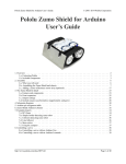
Thomas Bräunl
EMBEDDED ROBOTICS
Mobile Robot Design
and Applications
with Embedded Systems
Second Edition
With 233 Figures and 24 Tables
123
Thomas Bräunl
School of Electrical, Electronic
and Computer Engineering
The University of Western Australia
35 Stirling Highway
Crawley, Perth, WA 6009
Australia
Library of Congress Control Number: 2006925479
ACM Computing Classification (1998): I.2.9, C.3
ISBN-10 3-540-34318-0 Springer Berlin Heidelberg New York
ISBN-13 978-3-540-34318-9 Springer Berlin Heidelberg New York
ISBN-10 3-540-03436-6 1. Edition Springer Berlin Heidelberg New York
This work is subject to copyright. All rights are reserved, whether the whole or part of the
PDWHULDOLVFRQFHUQHGVSHFL¿FDOO\WKHULJKWVRIWUDQVODWLRQUHSULQWLQJUHXVHRILOOXVWUDWLRQVUHFLWDWLRQEURDGFDVWLQJUHSURGXFWLRQRQPLFUR¿OPRULQDQ\RWKHUZD\DQGVWRUDJH
in data banks. Duplication of this publication or parts thereof is permitted only under the
provisions of the German Copyright Law of September 9, 1965, in its current version,
and permission for use must always be obtained from Springer. Violations are liable for
prosecution under the German Copyright Law.
Springer is a part of Springer Science+Business Media
springer.com
© Springer-Verlag Berlin Heidelberg 2003, 2006
Printed in Germany
The use of general descriptive names, registered names, trademarks, etc. in this publiFDWLRQGRHVQRWLPSO\HYHQLQWKHDEVHQFHRIDVSHFL¿FVWDWHPHQWWKDWVXFKQDPHVDUH
exempt from the relevant protective laws and regulations and therefore free for general
use.
Typesetting: Camera-ready by the author
Production: LE-TEX Jelonek, Schmidt &Vöckler GbR, Leipzig
Cover design: KünkelLopka, Heidelberg
P
REFACE
...................................
.........
I
t all started with a new robot lab course I had developed to accompany my
robotics lectures. We already had three large, heavy, and expensive
mobile robots for research projects, but nothing simple and safe, which we
could give to students to practice on for an introductory course.
We selected a mobile robot kit based on an 8-bit controller, and used it for
the first couple of years of this course. This gave students not only the enjoyment of working with real robots but, more importantly, hands-on experience
with control systems, real-time systems, concurrency, fault tolerance, sensor
and motor technology, etc. It was a very successful lab and was greatly
enjoyed by the students. Typical tasks were, for example, driving straight,
finding a light source, or following a leading vehicle. Since the robots were
rather inexpensive, it was possible to furnish a whole lab with them and to conduct multi-robot experiments as well.
Simplicity, however, had its drawbacks. The robot mechanics were unreliable, the sensors were quite poor, and extendability and processing power were
very limited. What we wanted to use was a similar robot at an advanced level.
The processing power had to be reasonably fast, it should use precision motors
and sensors, and – most challenging – the robot had to be able to do on-board
image processing. This had never been accomplished before on a robot of such
a small size (about 12cm u9cm u14cm). Appropriately, the robot project was
called “EyeBot”. It consisted of a full 32-bit controller (“EyeCon”), interfacing
directly to a digital camera (“EyeCam”) and a large graphics display for visual
feedback. A row of user buttons below the LCD was included as “soft keys” to
allow a simple user interface, which most other mobile robots lack. The
processing power of the controller is about 1,000 times faster than for robots
based on most 8-bit controllers (25MHz processor speed versus 1MHz, 32-bit
data width versus 8-bit, compiled C code versus interpretation) and this does
not even take into account special CPU features like the “time processor unit”
(TPU).
The EyeBot family includes several driving robots with differential steering, tracked vehicles, omni-directional vehicles, balancing robots, six-legged
walkers, biped android walkers, autonomous flying and underwater robots, as
VV
Preface
well as simulation systems for driving robots (“EyeSim”) and underwater
robots (“SubSim”). EyeCon controllers are used in several other projects, with
and without mobile robots. Numerous universities use EyeCons to drive their
own mobile robot creations. We use boxed EyeCons for experiments in a second-year course in Embedded Systems as part of the Electrical Engineering,
Information Technology, and Mechatronics curriculums. And one lonely EyeCon controller sits on a pole on Rottnest Island off the coast of Western Australia, taking care of a local weather station.
Acknowledgements
While the controller hardware and robot mechanics were developed commercially, several universities and numerous students contributed to the EyeBot
software collection. The universities involved in the EyeBot project are:
•
•
•
•
•
•
University of Stuttgart, Germany
University of Kaiserslautern, Germany
Rochester Institute of Technology, USA
The University of Auckland, New Zealand
The University of Manitoba, Winnipeg, Canada
The University of Western Australia (UWA), Perth, Australia
The author would like to thank the following students, technicians, and
colleagues: Gerrit Heitsch, Thomas Lampart, Jörg Henne, Frank Sautter, Elliot
Nicholls, Joon Ng, Jesse Pepper, Richard Meager, Gordon Menck, Andrew
McCandless, Nathan Scott, Ivan Neubronner, Waldemar Spädt, Petter
Reinholdtsen, Birgit Graf, Michael Kasper, Jacky Baltes, Peter Lawrence, Nan
Schaller, Walter Bankes, Barb Linn, Jason Foo, Alistair Sutherland, Joshua
Petitt, Axel Waggershauser, Alexandra Unkelbach, Martin Wicke, Tee Yee
Ng, Tong An, Adrian Boeing, Courtney Smith, Nicholas Stamatiou, Jonathan
Purdie, Jippy Jungpakdee, Daniel Venkitachalam, Tommy Cristobal, Sean
Ong, and Klaus Schmitt.
Thanks for proofreading the manuscript and numerous suggestions go to
Marion Baer, Linda Barbour, Adrian Boeing, Michael Kasper, Joshua Petitt,
Klaus Schmitt, Sandra Snook, Anthony Zaknich, and everyone at SpringerVerlag.
Contributions
A number of colleagues and former students contributed to this book. The
author would like to thank everyone for their effort in putting the material
together.
JACKY BALTES
VI
The University of Manitoba, Winnipeg, contributed to the
section on PID control,
Preface
ADRIAN BOEING
UWA, coauthored the chapters on the evolution of walking gaits and genetic algorithms, and contributed to the
section on SubSim,
CHRISTOPH BRAUNSCHÄDEL FH Koblenz, contributed data plots to the sections on PID control and on/off control,
MICHAEL DRTIL
FH Koblenz, contributed to the chapter on AUVs,
LOUIS GONZALEZ UWA, contributed to the chapter on AUVs,
BIRGIT GRAF
Fraunhofer IPA, Stuttgart, coauthored the chapter on robot
soccer,
HIROYUKI HARADA Hokkaido University, Sapporo, contributed the visualization diagrams to the section on biped robot design,
YVES HWANG
UWA, coauthored the chapter on genetic programming,
PHILIPPE LECLERCQ UWA, contributed to the section on color segmentation,
JAMES NG
UWA, coauthored the sections on probabilistic localization and the DistBug navigation algorithm.
JOSHUA PETITT
UWA, contributed to the section on DC motors,
KLAUS SCHMITT
Univ. Kaiserslautern, coauthored the section on the RoBIOS operating system,
ALISTAIR SUTHERLAND UWA, coauthored the chapter on balancing robots,
NICHOLAS TAY
DSTO, Canberra, coauthored the chapter on map generation,
DANIEL VENKITACHALAM UWA, coauthored the chapters on genetic algorithms and behavior-based systems and contributed to the
chapter on neural networks,
EYESIM was implemented by Axel Waggershauser (V5) and Andreas Koestler
(V6), UWA, Univ. Kaiserslautern, and FH Giessen.
SUBSIM was implemented by Adrian Boeing, Andreas Koestler, and Joshua
Petitt (V1), and Thorsten Rühl and Tobias Bielohlawek
(V2), UWA, FH Giessen, and Univ. Kaiserslautern.
Additional Material
Hardware and mechanics of the “EyeCon” controller and various robots of the
EyeBot family are available from INROSOFT and various distributors:
http://inrosoft.com
All system software discussed in this book, the RoBIOS operating system,
C/C++ compilers for Linux and Windows, system tools, image processing
tools, simulation system, and a large collection of example programs are available free from:
http://robotics.ee.uwa.edu.au/eyebot/
VII
Preface
Lecturers who adopt this book for a course can receive a full set of the
author’s course notes (PowerPoint slides), tutorials, and labs from this website.
And finally, if you have developed some robot application programs you
would like to share, please feel free to submit them to our website.
Second Edition
Less than three years have passed since this book was first published and I
have since used this book successfully in courses on Embedded Systems and
on Mobile Robots / Intelligent Systems. Both courses are accompanied by
hands-on lab sessions using the EyeBot controllers and robot systems, which
the students found most interesting and which I believe contribute significantly
to the learning process.
What started as a few minor changes and corrections to the text, turned into
a major rework and additional material has been added in several areas. A new
chapter on autonomous vessels and underwater vehicles and a new section on
AUV simulation have been added, the material on localization and navigation
has been extended and moved to a separate chapter, and the kinematics sections for driving and omni-directional robots have been updated, while a couple of chapters have been shifted to the Appendix.
Again, I would like to thank all students and visitors who conducted
research and development work in my lab and contributed to this book in one
form or another.
All software presented in this book, especially the EyeSim and SubSim
simulation systems can be freely downloaded from:
http://robotics.ee.uwa.edu.au
Perth, Australia, June 2006
VIII
Thomas Bräunl
C
ONTENTS
...................................
.........
PART I: EMBEDDED SYSTEMS
1
Robots and Controllers
1.1
1.2
1.3
1.4
1.5
2
Sensors
2.1
2.2
2.3
2.4
2.5
2.6
2.7
2.8
2.9
2.10
3
4
41
DC Motors . . . . . . . . . . . . . . . . . . . . . . . . . . . . . . . . . . . . . . . . . . . . . . . . . . . . . 41
H-Bridge . . . . . . . . . . . . . . . . . . . . . . . . . . . . . . . . . . . . . . . . . . . . . . . . . . . . . . 44
Pulse Width Modulation . . . . . . . . . . . . . . . . . . . . . . . . . . . . . . . . . . . . . . . . . . 46
Stepper Motors. . . . . . . . . . . . . . . . . . . . . . . . . . . . . . . . . . . . . . . . . . . . . . . . . . 48
Servos . . . . . . . . . . . . . . . . . . . . . . . . . . . . . . . . . . . . . . . . . . . . . . . . . . . . . . . . 49
References . . . . . . . . . . . . . . . . . . . . . . . . . . . . . . . . . . . . . . . . . . . . . . . . . . . . . 50
Control
4.1
4.2
4.3
4.4
4.5
4.6
17
Sensor Categories . . . . . . . . . . . . . . . . . . . . . . . . . . . . . . . . . . . . . . . . . . . . . . . 18
Binary Sensor. . . . . . . . . . . . . . . . . . . . . . . . . . . . . . . . . . . . . . . . . . . . . . . . . . . 19
Analog versus Digital Sensors. . . . . . . . . . . . . . . . . . . . . . . . . . . . . . . . . . . . . . 19
Shaft Encoder. . . . . . . . . . . . . . . . . . . . . . . . . . . . . . . . . . . . . . . . . . . . . . . . . . . 20
A/D Converter . . . . . . . . . . . . . . . . . . . . . . . . . . . . . . . . . . . . . . . . . . . . . . . . . . 22
Position Sensitive Device . . . . . . . . . . . . . . . . . . . . . . . . . . . . . . . . . . . . . . . . . 23
Compass. . . . . . . . . . . . . . . . . . . . . . . . . . . . . . . . . . . . . . . . . . . . . . . . . . . . . . . 25
Gyroscope, Accelerometer, Inclinometer . . . . . . . . . . . . . . . . . . . . . . . . . . . . . 27
Digital Camera. . . . . . . . . . . . . . . . . . . . . . . . . . . . . . . . . . . . . . . . . . . . . . . . . . 30
References . . . . . . . . . . . . . . . . . . . . . . . . . . . . . . . . . . . . . . . . . . . . . . . . . . . . . 38
Actuators
3.1
3.2
3.3
3.4
3.5
3.6
3
Mobile Robots . . . . . . . . . . . . . . . . . . . . . . . . . . . . . . . . . . . . . . . . . . . . . . . . . . . 4
Embedded Controllers . . . . . . . . . . . . . . . . . . . . . . . . . . . . . . . . . . . . . . . . . . . . . 7
Interfaces . . . . . . . . . . . . . . . . . . . . . . . . . . . . . . . . . . . . . . . . . . . . . . . . . . . . . . 10
Operating System. . . . . . . . . . . . . . . . . . . . . . . . . . . . . . . . . . . . . . . . . . . . . . . . 13
References . . . . . . . . . . . . . . . . . . . . . . . . . . . . . . . . . . . . . . . . . . . . . . . . . . . . . 15
51
On-Off Control . . . . . . . . . . . . . . . . . . . . . . . . . . . . . . . . . . . . . . . . . . . . . . . . . 51
PID Control . . . . . . . . . . . . . . . . . . . . . . . . . . . . . . . . . . . . . . . . . . . . . . . . . . . . 56
Velocity Control and Position Control . . . . . . . . . . . . . . . . . . . . . . . . . . . . . . . 62
Multiple Motors – Driving Straight . . . . . . . . . . . . . . . . . . . . . . . . . . . . . . . . . 63
V-Omega Interface . . . . . . . . . . . . . . . . . . . . . . . . . . . . . . . . . . . . . . . . . . . . . . 66
References . . . . . . . . . . . . . . . . . . . . . . . . . . . . . . . . . . . . . . . . . . . . . . . . . . . . . 68
IXIX
Contents
5
Multitasking
5.1
5.2
5.3
5.4
5.5
5.6
6
Wireless Communication
6.1
6.2
6.3
6.4
6.5
6.6
69
Cooperative Multitasking . . . . . . . . . . . . . . . . . . . . . . . . . . . . . . . . . . . . . . . . . 69
Preemptive Multitasking . . . . . . . . . . . . . . . . . . . . . . . . . . . . . . . . . . . . . . . . . . 71
Synchronization . . . . . . . . . . . . . . . . . . . . . . . . . . . . . . . . . . . . . . . . . . . . . . . . . 73
Scheduling . . . . . . . . . . . . . . . . . . . . . . . . . . . . . . . . . . . . . . . . . . . . . . . . . . . . . 77
Interrupts and Timer-Activated Tasks . . . . . . . . . . . . . . . . . . . . . . . . . . . . . . . . 80
References . . . . . . . . . . . . . . . . . . . . . . . . . . . . . . . . . . . . . . . . . . . . . . . . . . . . . 82
83
Communication Model . . . . . . . . . . . . . . . . . . . . . . . . . . . . . . . . . . . . . . . . . . . 84
Messages . . . . . . . . . . . . . . . . . . . . . . . . . . . . . . . . . . . . . . . . . . . . . . . . . . . . . . 86
Fault-Tolerant Self-Configuration . . . . . . . . . . . . . . . . . . . . . . . . . . . . . . . . . . . 87
User Interface and Remote Control . . . . . . . . . . . . . . . . . . . . . . . . . . . . . . . . . . 89
Sample Application Program. . . . . . . . . . . . . . . . . . . . . . . . . . . . . . . . . . . . . . . 92
References . . . . . . . . . . . . . . . . . . . . . . . . . . . . . . . . . . . . . . . . . . . . . . . . . . . . . 93
PART II: MOBILE ROBOT DESIGN
7
Driving Robots
7.1
7.2
7.3
7.4
7.5
7.6
7.7
8
Omni-Directional Robots
8.1
8.2
8.3
8.4
8.5
8.6
9
X
123
Simulation . . . . . . . . . . . . . . . . . . . . . . . . . . . . . . . . . . . . . . . . . . . . . . . . . . . . 123
Inverted Pendulum Robot . . . . . . . . . . . . . . . . . . . . . . . . . . . . . . . . . . . . . . . . 124
Double Inverted Pendulum . . . . . . . . . . . . . . . . . . . . . . . . . . . . . . . . . . . . . . . 128
References . . . . . . . . . . . . . . . . . . . . . . . . . . . . . . . . . . . . . . . . . . . . . . . . . . . . 129
10 Walking Robots
10.1
10.2
10.3
10.4
113
Mecanum Wheels . . . . . . . . . . . . . . . . . . . . . . . . . . . . . . . . . . . . . . . . . . . . . . 113
Omni-Directional Drive. . . . . . . . . . . . . . . . . . . . . . . . . . . . . . . . . . . . . . . . . . 115
Kinematics . . . . . . . . . . . . . . . . . . . . . . . . . . . . . . . . . . . . . . . . . . . . . . . . . . . . 117
Omni-Directional Robot Design . . . . . . . . . . . . . . . . . . . . . . . . . . . . . . . . . . . 118
Driving Program . . . . . . . . . . . . . . . . . . . . . . . . . . . . . . . . . . . . . . . . . . . . . . . 119
References . . . . . . . . . . . . . . . . . . . . . . . . . . . . . . . . . . . . . . . . . . . . . . . . . . . . 120
Balancing Robots
9.1
9.2
9.3
9.4
97
Single Wheel Drive . . . . . . . . . . . . . . . . . . . . . . . . . . . . . . . . . . . . . . . . . . . . . . 97
Differential Drive. . . . . . . . . . . . . . . . . . . . . . . . . . . . . . . . . . . . . . . . . . . . . . . . 98
Tracked Robots . . . . . . . . . . . . . . . . . . . . . . . . . . . . . . . . . . . . . . . . . . . . . . . . 102
Synchro-Drive . . . . . . . . . . . . . . . . . . . . . . . . . . . . . . . . . . . . . . . . . . . . . . . . . 103
Ackermann Steering . . . . . . . . . . . . . . . . . . . . . . . . . . . . . . . . . . . . . . . . . . . . 105
Drive Kinematics . . . . . . . . . . . . . . . . . . . . . . . . . . . . . . . . . . . . . . . . . . . . . . 107
References . . . . . . . . . . . . . . . . . . . . . . . . . . . . . . . . . . . . . . . . . . . . . . . . . . . . 111
131
Six-Legged Robot Design . . . . . . . . . . . . . . . . . . . . . . . . . . . . . . . . . . . . . . . . 131
Biped Robot Design. . . . . . . . . . . . . . . . . . . . . . . . . . . . . . . . . . . . . . . . . . . . . 134
Sensors for Walking Robots . . . . . . . . . . . . . . . . . . . . . . . . . . . . . . . . . . . . . . 139
Static Balance . . . . . . . . . . . . . . . . . . . . . . . . . . . . . . . . . . . . . . . . . . . . . . . . . 140
Contents
10.5 Dynamic Balance. . . . . . . . . . . . . . . . . . . . . . . . . . . . . . . . . . . . . . . . . . . . . . . 143
10.6 References . . . . . . . . . . . . . . . . . . . . . . . . . . . . . . . . . . . . . . . . . . . . . . . . . . . . 148
11 Autonomous Planes
11.1
11.2
11.3
11.4
12 Autonomous Vessels and Underwater Vehicles
12.1
12.2
12.3
12.4
12.5
161
Application . . . . . . . . . . . . . . . . . . . . . . . . . . . . . . . . . . . . . . . . . . . . . . . . . . . 161
Dynamic Model . . . . . . . . . . . . . . . . . . . . . . . . . . . . . . . . . . . . . . . . . . . . . . . . 163
AUV Design Mako . . . . . . . . . . . . . . . . . . . . . . . . . . . . . . . . . . . . . . . . . . . . . 163
AUV Design USAL . . . . . . . . . . . . . . . . . . . . . . . . . . . . . . . . . . . . . . . . . . . . . 167
References . . . . . . . . . . . . . . . . . . . . . . . . . . . . . . . . . . . . . . . . . . . . . . . . . . . . 170
13 Simulation Systems
13.1
13.2
13.3
13.4
13.5
13.6
13.7
13.8
13.9
13.10
151
Application . . . . . . . . . . . . . . . . . . . . . . . . . . . . . . . . . . . . . . . . . . . . . . . . . . . 151
Control System and Sensors . . . . . . . . . . . . . . . . . . . . . . . . . . . . . . . . . . . . . . 154
Flight Program . . . . . . . . . . . . . . . . . . . . . . . . . . . . . . . . . . . . . . . . . . . . . . . . . 155
References . . . . . . . . . . . . . . . . . . . . . . . . . . . . . . . . . . . . . . . . . . . . . . . . . . . . 159
171
Mobile Robot Simulation . . . . . . . . . . . . . . . . . . . . . . . . . . . . . . . . . . . . . . . . 171
EyeSim Simulation System . . . . . . . . . . . . . . . . . . . . . . . . . . . . . . . . . . . . . . . 172
Multiple Robot Simulation . . . . . . . . . . . . . . . . . . . . . . . . . . . . . . . . . . . . . . . 177
EyeSim Application. . . . . . . . . . . . . . . . . . . . . . . . . . . . . . . . . . . . . . . . . . . . . 178
EyeSim Environment and Parameter Files . . . . . . . . . . . . . . . . . . . . . . . . . . . 179
SubSim Simulation System . . . . . . . . . . . . . . . . . . . . . . . . . . . . . . . . . . . . . . . 184
Actuator and Sensor Models . . . . . . . . . . . . . . . . . . . . . . . . . . . . . . . . . . . . . . 186
SubSim Application. . . . . . . . . . . . . . . . . . . . . . . . . . . . . . . . . . . . . . . . . . . . . 188
SubSim Environment and Parameter Files . . . . . . . . . . . . . . . . . . . . . . . . . . . 190
References . . . . . . . . . . . . . . . . . . . . . . . . . . . . . . . . . . . . . . . . . . . . . . . . . . . . 193
PART III: MOBILE ROBOT APPLICATIONS
14 Localization and Navigation
14.1
14.2
14.3
14.4
14.5
14.6
14.7
14.8
14.9
15 Maze Exploration
15.1
15.2
15.3
15.4
197
Localization . . . . . . . . . . . . . . . . . . . . . . . . . . . . . . . . . . . . . . . . . . . . . . . . . . . 197
Probabilistic Localization . . . . . . . . . . . . . . . . . . . . . . . . . . . . . . . . . . . . . . . . 201
Coordinate Systems . . . . . . . . . . . . . . . . . . . . . . . . . . . . . . . . . . . . . . . . . . . . . 205
Dijkstra’s Algorithm . . . . . . . . . . . . . . . . . . . . . . . . . . . . . . . . . . . . . . . . . . . . 206
A* Algorithm. . . . . . . . . . . . . . . . . . . . . . . . . . . . . . . . . . . . . . . . . . . . . . . . . . 210
Potential Field Method . . . . . . . . . . . . . . . . . . . . . . . . . . . . . . . . . . . . . . . . . . 211
Wandering Standpoint Algorithm . . . . . . . . . . . . . . . . . . . . . . . . . . . . . . . . . . 212
DistBug Algorithm . . . . . . . . . . . . . . . . . . . . . . . . . . . . . . . . . . . . . . . . . . . . . 213
References . . . . . . . . . . . . . . . . . . . . . . . . . . . . . . . . . . . . . . . . . . . . . . . . . . . . 215
217
Micro Mouse Contest . . . . . . . . . . . . . . . . . . . . . . . . . . . . . . . . . . . . . . . . . . . 217
Maze Exploration Algorithms . . . . . . . . . . . . . . . . . . . . . . . . . . . . . . . . . . . . . 219
Simulated versus Real Maze Program . . . . . . . . . . . . . . . . . . . . . . . . . . . . . . . 226
References . . . . . . . . . . . . . . . . . . . . . . . . . . . . . . . . . . . . . . . . . . . . . . . . . . . . 228
XIXI
Contents
16 Map Generation
16.1
16.2
16.3
16.4
16.5
16.6
16.7
16.8
17 Real-Time Image Processing
17.1
17.2
17.3
17.4
17.5
17.6
17.7
17.8
17.9
XII
277
Neural Network Principles . . . . . . . . . . . . . . . . . . . . . . . . . . . . . . . . . . . . . . . 277
Feed-Forward Networks . . . . . . . . . . . . . . . . . . . . . . . . . . . . . . . . . . . . . . . . . 278
Backpropagation . . . . . . . . . . . . . . . . . . . . . . . . . . . . . . . . . . . . . . . . . . . . . . . 283
Neural Network Example . . . . . . . . . . . . . . . . . . . . . . . . . . . . . . . . . . . . . . . . 288
Neural Controller . . . . . . . . . . . . . . . . . . . . . . . . . . . . . . . . . . . . . . . . . . . . . . . 289
References . . . . . . . . . . . . . . . . . . . . . . . . . . . . . . . . . . . . . . . . . . . . . . . . . . . . 290
20 Genetic Algorithms
20.1
20.2
20.3
20.4
20.5
20.6
263
RoboCup and FIRA Competitions. . . . . . . . . . . . . . . . . . . . . . . . . . . . . . . . . . 263
Team Structure. . . . . . . . . . . . . . . . . . . . . . . . . . . . . . . . . . . . . . . . . . . . . . . . . 266
Mechanics and Actuators. . . . . . . . . . . . . . . . . . . . . . . . . . . . . . . . . . . . . . . . . 267
Sensing. . . . . . . . . . . . . . . . . . . . . . . . . . . . . . . . . . . . . . . . . . . . . . . . . . . . . . . 267
Image Processing . . . . . . . . . . . . . . . . . . . . . . . . . . . . . . . . . . . . . . . . . . . . . . . 269
Trajectory Planning . . . . . . . . . . . . . . . . . . . . . . . . . . . . . . . . . . . . . . . . . . . . . 271
References . . . . . . . . . . . . . . . . . . . . . . . . . . . . . . . . . . . . . . . . . . . . . . . . . . . . 276
19 Neural Networks
19.1
19.2
19.3
19.4
19.5
19.6
243
Camera Interface . . . . . . . . . . . . . . . . . . . . . . . . . . . . . . . . . . . . . . . . . . . . . . . 243
Auto-Brightness . . . . . . . . . . . . . . . . . . . . . . . . . . . . . . . . . . . . . . . . . . . . . . . . 245
Edge Detection. . . . . . . . . . . . . . . . . . . . . . . . . . . . . . . . . . . . . . . . . . . . . . . . . 246
Motion Detection . . . . . . . . . . . . . . . . . . . . . . . . . . . . . . . . . . . . . . . . . . . . . . . 248
Color Space . . . . . . . . . . . . . . . . . . . . . . . . . . . . . . . . . . . . . . . . . . . . . . . . . . . 249
Color Object Detection . . . . . . . . . . . . . . . . . . . . . . . . . . . . . . . . . . . . . . . . . . 251
Image Segmentation . . . . . . . . . . . . . . . . . . . . . . . . . . . . . . . . . . . . . . . . . . . . 256
Image Coordinates versus World Coordinates . . . . . . . . . . . . . . . . . . . . . . . . 258
References . . . . . . . . . . . . . . . . . . . . . . . . . . . . . . . . . . . . . . . . . . . . . . . . . . . . 260
18 Robot Soccer
18.1
18.2
18.3
18.4
18.5
18.6
18.7
229
Mapping Algorithm . . . . . . . . . . . . . . . . . . . . . . . . . . . . . . . . . . . . . . . . . . . . . 229
Data Representation. . . . . . . . . . . . . . . . . . . . . . . . . . . . . . . . . . . . . . . . . . . . . 231
Boundary-Following Algorithm . . . . . . . . . . . . . . . . . . . . . . . . . . . . . . . . . . . 232
Algorithm Execution . . . . . . . . . . . . . . . . . . . . . . . . . . . . . . . . . . . . . . . . . . . . 233
Simulation Experiments. . . . . . . . . . . . . . . . . . . . . . . . . . . . . . . . . . . . . . . . . . 235
Robot Experiments . . . . . . . . . . . . . . . . . . . . . . . . . . . . . . . . . . . . . . . . . . . . . 236
Results . . . . . . . . . . . . . . . . . . . . . . . . . . . . . . . . . . . . . . . . . . . . . . . . . . . . . . . 239
References . . . . . . . . . . . . . . . . . . . . . . . . . . . . . . . . . . . . . . . . . . . . . . . . . . . . 240
291
Genetic Algorithm Principles . . . . . . . . . . . . . . . . . . . . . . . . . . . . . . . . . . . . . 292
Genetic Operators . . . . . . . . . . . . . . . . . . . . . . . . . . . . . . . . . . . . . . . . . . . . . . 294
Applications to Robot Control. . . . . . . . . . . . . . . . . . . . . . . . . . . . . . . . . . . . . 296
Example Evolution . . . . . . . . . . . . . . . . . . . . . . . . . . . . . . . . . . . . . . . . . . . . . 297
Implementation of Genetic Algorithms . . . . . . . . . . . . . . . . . . . . . . . . . . . . . . 301
References . . . . . . . . . . . . . . . . . . . . . . . . . . . . . . . . . . . . . . . . . . . . . . . . . . . . 304
Contents
21 Genetic Programming
21.1
21.2
21.3
21.4
21.5
21.6
21.7
22 Behavior-Based Systems
22.1
22.2
22.3
22.4
22.5
22.6
22.7
22.8
22.9
325
Software Architecture . . . . . . . . . . . . . . . . . . . . . . . . . . . . . . . . . . . . . . . . . . . 325
Behavior-Based Robotics . . . . . . . . . . . . . . . . . . . . . . . . . . . . . . . . . . . . . . . . 326
Behavior-Based Applications . . . . . . . . . . . . . . . . . . . . . . . . . . . . . . . . . . . . . 329
Behavior Framework . . . . . . . . . . . . . . . . . . . . . . . . . . . . . . . . . . . . . . . . . . . . 330
Adaptive Controller . . . . . . . . . . . . . . . . . . . . . . . . . . . . . . . . . . . . . . . . . . . . . 333
Tracking Problem . . . . . . . . . . . . . . . . . . . . . . . . . . . . . . . . . . . . . . . . . . . . . . 337
Neural Network Controller . . . . . . . . . . . . . . . . . . . . . . . . . . . . . . . . . . . . . . . 338
Experiments . . . . . . . . . . . . . . . . . . . . . . . . . . . . . . . . . . . . . . . . . . . . . . . . . . . 340
References . . . . . . . . . . . . . . . . . . . . . . . . . . . . . . . . . . . . . . . . . . . . . . . . . . . . 342
23 Evolution of Walking Gaits
23.1
23.2
23.3
23.4
23.5
23.6
23.7
307
Concepts and Applications . . . . . . . . . . . . . . . . . . . . . . . . . . . . . . . . . . . . . . . 307
Lisp . . . . . . . . . . . . . . . . . . . . . . . . . . . . . . . . . . . . . . . . . . . . . . . . . . . . . . . . . 309
Genetic Operators . . . . . . . . . . . . . . . . . . . . . . . . . . . . . . . . . . . . . . . . . . . . . . 313
Evolution . . . . . . . . . . . . . . . . . . . . . . . . . . . . . . . . . . . . . . . . . . . . . . . . . . . . . 315
Tracking Problem . . . . . . . . . . . . . . . . . . . . . . . . . . . . . . . . . . . . . . . . . . . . . . 316
Evolution of Tracking Behavior . . . . . . . . . . . . . . . . . . . . . . . . . . . . . . . . . . . 319
References . . . . . . . . . . . . . . . . . . . . . . . . . . . . . . . . . . . . . . . . . . . . . . . . . . . . 323
345
Splines . . . . . . . . . . . . . . . . . . . . . . . . . . . . . . . . . . . . . . . . . . . . . . . . . . . . . . . 345
Control Algorithm . . . . . . . . . . . . . . . . . . . . . . . . . . . . . . . . . . . . . . . . . . . . . . 346
Incorporating Feedback . . . . . . . . . . . . . . . . . . . . . . . . . . . . . . . . . . . . . . . . . . 348
Controller Evolution . . . . . . . . . . . . . . . . . . . . . . . . . . . . . . . . . . . . . . . . . . . . 349
Controller Assessment . . . . . . . . . . . . . . . . . . . . . . . . . . . . . . . . . . . . . . . . . . . 351
Evolved Gaits. . . . . . . . . . . . . . . . . . . . . . . . . . . . . . . . . . . . . . . . . . . . . . . . . . 352
References . . . . . . . . . . . . . . . . . . . . . . . . . . . . . . . . . . . . . . . . . . . . . . . . . . . . 355
24 Outlook
357
APPENDICES
A
B
C
D
E
F
Programming Tools . . . . . . . . . . . . . . . . . . . . . . . . . . . . . . . . . . . . . . . . . . . . . . . . . . 361
RoBIOS Operating System . . . . . . . . . . . . . . . . . . . . . . . . . . . . . . . . . . . . . . . . . . . . 371
Hardware Description Table . . . . . . . . . . . . . . . . . . . . . . . . . . . . . . . . . . . . . . . . . . . 413
Hardware Specification . . . . . . . . . . . . . . . . . . . . . . . . . . . . . . . . . . . . . . . . . . . . . . . 429
Laboratories . . . . . . . . . . . . . . . . . . . . . . . . . . . . . . . . . . . . . . . . . . . . . . . . . . . . . . . . 437
Solutions. . . . . . . . . . . . . . . . . . . . . . . . . . . . . . . . . . . . . . . . . . . . . . . . . . . . . . . . . . . 447
Index
451
XIIIXIII
PART I:
E
MBEDDED SYSTEMS
...................................
.........
11
ROBOTS AND
C
ONTROLLERS
...................................
.........
R
1
obotics has come a long way. Especially for mobile robots, a similar
trend is happening as we have seen for computer systems: the transition from mainframe computing via workstations to PCs, which will
probably continue with handheld devices for many applications. In the past,
mobile robots were controlled by heavy, large, and expensive computer systems that could not be carried and had to be linked via cable or wireless
devices. Today, however, we can build small mobile robots with numerous
actuators and sensors that are controlled by inexpensive, small, and light
embedded computer systems that are carried on-board the robot.
There has been a tremendous increase of interest in mobile robots. Not just
as interesting toys or inspired by science fiction stories or movies [Asimov
1950], but as a perfect tool for engineering education, mobile robots are used
today at almost all universities in undergraduate and graduate courses in Computer Science/Computer Engineering, Information Technology, Cybernetics,
Electrical Engineering, Mechanical Engineering, and Mechatronics.
What are the advantages of using mobile robot systems as opposed to traditional ways of education, for example mathematical models or computer simulation?
First of all, a robot is a tangible, self-contained piece of real-world hardware. Students can relate to a robot much better than to a piece of software.
Tasks to be solved involving a robot are of a practical nature and directly
“make sense” to students, much more so than, for example, the inevitable comparison of sorting algorithms.
Secondly, all problems involving “real-world hardware” such as a robot, are
in many ways harder than solving a theoretical problem. The “perfect world”
which often is the realm of pure software systems does not exist here. Any
actuator can only be positioned to a certain degree of accuracy, and all sensors
have intrinsic reading errors and certain limitations. Therefore, a working
robot program will be much more than just a logic solution coded in software.
33
1
Robots and Controllers
It will be a robust system that takes into account and overcomes inaccuracies
and imperfections. In summary: a valid engineering approach to a typical
(industrial) problem.
Third and finally, mobile robot programming is enjoyable and an inspiration to students. The fact that there is a moving system whose behavior can be
specified by a piece of software is a challenge. This can even be amplified by
introducing robot competitions where two teams of robots compete in solving
a particular task [Bräunl 1999] – achieving a goal with autonomously operating robots, not remote controlled destructive “robot wars”.
1.1 Mobile Robots
Since the foundation of the Mobile Robot Lab by the author at The University
of Western Australia in 1998, we have developed a number of mobile robots,
including wheeled, tracked, legged, flying, and underwater robots. We call
these robots the “EyeBot family” of mobile robots (Figure 1.1), because they
are all using the same embedded controller “EyeCon” (EyeBot controller, see
the following section).
Figure 1.1: Some members of the EyeBot family of mobile robots
The simplest case of mobile robots are wheeled robots, as shown in Figure
1.2. Wheeled robots comprise one or more driven wheels (drawn solid in the
figure) and have optional passive or caster wheels (drawn hollow) and possibly steered wheels (drawn inside a circle). Most designs require two motors for
driving (and steering) a mobile robot.
The design on the left-hand side of Figure 1.2 has a single driven wheel that
is also steered. It requires two motors, one for driving the wheel and one for
turning. The advantage of this design is that the driving and turning actions
4
Mobile Robots
Figure 1.2: Wheeled robots
have been completely separated by using two different motors. Therefore, the
control software for driving curves will be very simple. A disadvantage of this
design is that the robot cannot turn on the spot, since the driven wheel is not
located at its center.
The robot design in the middle of Figure 1.2 is called “differential drive”
and is one of the most commonly used mobile robot designs. The combination
of two driven wheels allows the robot to be driven straight, in a curve, or to
turn on the spot. The translation between driving commands, for example a
curve of a given radius, and the corresponding wheel speeds has to be done
using software. Another advantage of this design is that motors and wheels are
in fixed positions and do not need to be turned as in the previous design. This
simplifies the robot mechanics design considerably.
Finally, on the right-hand side of Figure 1.2 is the so-called “Ackermann
Steering”, which is the standard drive and steering system of a rear-driven passenger car. We have one motor for driving both rear wheels via a differential
box and one motor for combined steering of both front wheels.
It is interesting to note that all of these different mobile robot designs
require two motors in total for driving and steering.
A special case of a wheeled robot is the omni-directional “Mecanum drive”
robot in Figure 1.3, left. It uses four driven wheels with a special wheel design
and will be discussed in more detail in a later chapter.
Figure 1.3: Omni-directional, tracked, and walking robots
One disadvantage of all wheeled robots is that they require a street or some
sort of flat surface for driving. Tracked robots (see Figure 1.3, middle) are
more flexible and can navigate over rough terrain. However, they cannot navigate as accurately as a wheeled robot. Tracked robots also need two motors,
one for each track.
5
1
Braitenberg
vehicles
Robots and Controllers
Legged robots (see Figure 1.3, right) are the final category of land-based
mobile robots. Like tracked robots, they can navigate over rough terrain or
climb up and down stairs, for example. There are many different designs for
legged robots, depending on their number of legs. The general rule is: the more
legs, the easier to balance. For example, the six-legged robot shown in the figure can be operated in such a way that three legs are always on the ground
while three legs are in the air. The robot will be stable at all times, resting on a
tripod formed from the three legs currently on the ground – provided its center
of mass falls in the triangle described by these three legs. The less legs a robot
has, the more complex it gets to balance and walk, for example a robot with
only four legs needs to be carefully controlled, in order not to fall over. A
biped (two-legged) robot cannot play the same trick with a supporting triangle,
since that requires at least three legs. So other techniques for balancing need to
be employed, as is discussed in greater detail in Chapter 10. Legged robots
usually require two or more motors (“degrees of freedom”) per leg, so a sixlegged robot requires at least 12 motors. Many biped robot designs have five
or more motors per leg, which results in a rather large total number of degrees
of freedom and also in considerable weight and cost.
A very interesting conceptual abstraction of actuators, sensors, and robot
control is the vehicles described by Braitenberg [Braitenberg 1984]. In one
example, we have a simple interaction between motors and light sensors. If a
light sensor is activated by a light source, it will proportionally increase the
speed of the motor it is linked to.
Figure 1.4: Braitenberg vehicles avoiding light (phototroph)
In Figure 1.4 our robot has two light sensors, one on the front left, one on
the front right. The left light sensor is linked to the left motor, the right sensor
to the right motor. If a light source appears in front of the robot, it will start
driving toward it, because both sensors will activate both motors. However,
what happens if the robot gets closer to the light source and goes slightly off
course? In this case, one of the sensors will be closer to the light source (the
left sensor in the figure), and therefore one of the motors (the left motor in the
figure) will become faster than the other. This will result in a curve trajectory
of our robot and it will miss the light source.
6
Embedded Controllers
Figure 1.5: Braitenberg vehicles searching light (photovore)
Figure 1.5 shows a very similar scenario of Braitenberg vehicles. However,
here we have linked the left sensor to the right motor and the right sensor to the
left motor. If we conduct the same experiment as before, again the robot will
start driving when encountering a light source. But when it gets closer and also
slightly off course (veering to the right in the figure), the left sensor will now
receive more light and therefore accelerate the right motor. This will result in a
left curve, so the robot is brought back on track to find the light source.
Braitenberg vehicles are only a limited abstraction of robots. However, a
number of control concepts can easily be demonstrated by using them.
1.2 Embedded Controllers
The centerpiece of all our robot designs is a small and versatile embedded controller that each robot carries on-board. We called it the “EyeCon” (EyeBot
controller, Figure 1.6), since its chief specification was to provide an interface
for a digital camera in order to drive a mobile robot using on-board image
processing [Bräunl 2001].
Figure 1.6: EyeCon, front and with camera attached
7
1
Robots and Controllers
The EyeCon is a small, light, and fully self-contained embedded controller.
It combines a 32bit CPU with a number of standard interfaces and drivers for
DC motors, servos, several types of sensors, plus of course a digital color camera. Unlike most other controllers, the EyeCon comes with a complete built-in
user interface: it comprises a large graphics display for displaying text messages and graphics, as well as four user input buttons. Also, a microphone and
a speaker are included. The main characteristics of the EyeCon are:
EyeCon specs
•
•
•
•
•
•
•
•
•
•
•
•
•
•
•
•
•
•
•
25MHz 32bit controller (Motorola M68332)
1MB RAM, extendable to 2MB
512KB ROM (for system + user programs)
1 Parallel port
3 Serial ports (1 at V24, 2 at TTL)
8 Digital inputs
8 Digital outputs
16 Timing processor unit inputs/outputs
8 Analog inputs
Single compact PCB
Interface for color and grayscale camera
Large graphics LCD (128u64 pixels)
4 input buttons
Reset button
Power switch
Audio output
• Piezo speaker
• Adapter and volume potentiometer for external speaker
Microphone for audio input
Battery level indication
Connectors for actuators and sensors:
• Digital camera
• 2 DC motors with encoders
• 12 Servos
• 6 Infrared sensors
• 6 Free analog inputs
One of the biggest achievements in designing hardware and software for the
EyeCon embedded controller was interfacing to a digital camera to allow onboard real-time image processing. We started with grayscale and color Connectix “QuickCam” camera modules for which interface specifications were
available. However, this was no longer the case for successor models and it is
virtually impossible to interface a camera if the manufacturer does not disclose
the protocol. This lead us to develop our own camera module “EyeCam” using
low resolution CMOS sensor chips. The current design includes a FIFO hardware buffer to increase the throughput of image data.
A number of simpler robots use only 8bit controllers [Jones, Flynn, Seiger
1999]. However, the major advantage of using a 32bit controller versus an 8bit
controller is not just its higher CPU frequency (about 25 times faster) and
8
Embedded Controllers
wider word format (4 times), but the ability to use standard off-the-shelf C and
C++ compilers. Compilation makes program execution about 10 times faster
than interpretation, so in total this results in a system that is 1,000 times faster.
We are using the GNU C/C++ cross-compiler for compiling both the operating
system and user application programs under Linux or Windows. This compiler
is the industry standard and highly reliable. It is not comparable with any of
the C-subset interpreters available.
The EyeCon embedded controller runs our own “RoBIOS” (Robot Basic
Input Output System) operating system that resides in the controller’s flashROM. This allows a very simple upgrade of a controller by simply downloading a new system file. It only requires a few seconds and no extra equipment,
since both the Motorola background debugger circuitry and the writeable
flash-ROM are already integrated into the controller.
RoBIOS combines a small monitor program for loading, storing, and executing programs with a library of user functions that control the operation of
all on-board and off-board devices (see Appendix B.5). The library functions
include displaying text/graphics on the LCD, reading push-button status, reading sensor data, reading digital images, reading robot position data, driving
motors, v-omega (vZ) driving interface, etc. Included also is a thread-based
multitasking system with semaphores for synchronization. The RoBIOS operating system is discussed in more detail in Chapter B.
Another important part of the EyeCon’s operating system is the HDT
(Hardware Description Table). This is a system table that can be loaded to
flash-ROM independent of the RoBIOS version. So it is possible to change the
system configuration by changing HDT entries, without touching the RoBIOS
operating system. RoBIOS can display the current HDT and allows selection
and testing of each system component listed (for example an infrared sensor or
a DC motor) by component-specific testing routines.
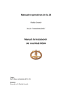
Figure 1.7 from [InroSoft 2006], the commercial producer of the EyeCon
controller, shows hardware schematics. Framed by the address and data buses
on the top and the chip-select lines on the bottom are the main system components ROM, RAM, and latches for digital I/O. The LCD module is memory
mapped, and therefore looks like a special RAM chip in the schematics.
Optional parts like the RAM extension are shaded in this diagram. The digital
camera can be interfaced through the parallel port or the optional FIFO buffer.
While the Motorola M68332 CPU on the left already provides one serial port,
we are using an ST16C552 to add a parallel port and two further serial ports to
the EyeCon system. Serial-1 is converted to V24 level (range +12V to –12V)
with the help of a MAX232 chip. This allows us to link this serial port directly
to any other device, such as a PC, Macintosh, or workstation for program
download. The other two serial ports, Serial-2 and Serial-3, stay at TTL level
(+5V) for linking other TTL-level communication hardware, such as the wireless module for Serial-2 and the IRDA wireless infrared module for Serial-3.
A number of CPU ports are hardwired to EyeCon system components; all
others can be freely assigned to sensors or actuators. By using the HDT, these
assignments can be defined in a structured way and are transparent to the user
9
1
Robots and Controllers
© InroSoft, Thomas Bräunl 2006
Figure 1.7: EyeCon schematics
program. The on-board motor controllers and feedback encoders utilize the
lower TPU channels plus some pins from the CPU port E, while the speaker
uses the highest TPU channel. Twelve TPU channels are provided with matching connectors for servos, i.e. model car/plane motors with pulse width modulation (PWM) control, so they can simply be plugged in and immediately operated. The input keys are linked to CPU port F, while infrared distance sensors
(PSDs, position sensitive devices) can be linked to either port E or some of the
digital inputs.
An eight-line analog to digital (A/D) converter is directly linked to the
CPU. One of its channels is used for the microphone, and one is used for the
battery status. The remaining six channels are free and can be used for connecting analog sensors.
1.3 Interfaces
A number of interfaces are available on most embedded systems. These are
digital inputs, digital outputs, and analog inputs. Analog outputs are not
always required and would also need additional amplifiers to drive any actuators. Instead, DC motors are usually driven by using a digital output line and a
pulsing technique called “pulse width modulation” (PWM). See Chapter 3 for
10
Interfaces
video out
camera connector IR receiver
serial 1
serial 2
graphics LCD
reset button
power switch
speaker microphone
input buttons
parallel port
motors and encoders (2)
background debugger
analog inputs
digital I/O
servos (14)
power
PSD (6) serial 3
Figure 1.8: EyeCon controller M5, front and back
details. The Motorola M68332 microcontroller already provides a number of
digital I/O lines, grouped together in ports. We are utilizing these CPU ports as
11
1
Robots and Controllers
can be seen in the schematics diagram Figure 1.7, but also provide additional
digital I/O pins through latches.
Most important is the M68332’s TPU. This is basically a second CPU integrated on the same chip, but specialized to timing tasks. It simplifies tremendously many time-related functions, like periodic signal generation or pulse
counting, which are frequently required for robotics applications.
Figure 1.8 shows the EyeCon board with all its components and interface
connections from the front and back. Our design objective was to make the
construction of a robot around the EyeCon as simple as possible. Most interface connectors allow direct plug-in of hardware components. No adapters or
special cables are required to plug servos, DC motors, or PSD sensors into the
EyeCon. Only the HDT software needs to be updated by simply downloading
the new configuration from a PC; then each user program can access the new
hardware.
The parallel port and the three serial ports are standard ports and can be
used to link to a host system, other controllers, or complex sensors/actuators.
Serial port 1 operates at V24 level, while the other two serial ports operate at
TTL level.
The Motorola background debugger (BDM) is a special feature of the
M68332 controller. Additional circuitry is included in the EyeCon, so only a
cable is required to activate the BDM from a host PC. The BDM can be used to
debug an assembly program using breakpoints, single step, and memory or
register display. It can also be used to initialize the flash-ROM if a new chip is
inserted or the operating system has been wiped by accident.
Figure 1.9: EyeBox units
12
Operating System
At The University of Western Australia, we are using a stand-alone, boxed
version of the EyeCon controller (“EyeBox” Figure 1.9) for lab experiments in
the Embedded Systems course. They are used for the first block of lab experiments until we switch to the EyeBot Labcars (Figure 7.5). See Appendix E for
a collection of lab experiments.
1.4 Operating System
Embedded systems can have anything between a complex real-time operating
system, such as Linux, or just the application program with no operating system, whatsoever. It all depends on the intended application area. For the EyeCon controller, we developed our own operating system RoBIOS (Robot Basic
Input Output System), which is a very lean real-time operating system that
provides a monitor program as user interface, system functions (including
multithreading, semaphores, timers), plus a comprehensive device driver
library for all kinds of robotics and embedded systems applications. This
includes serial/parallel communication, DC motors, servos, various sensors,
graphics/text output, and input buttons. Details are listed in Appendix B.5.
User input/output
RoBIOS
Monitor program
User program
RoBIOS Operating system + Library functions
HDT
Hardware
Robot mechanics,
actuators, and sensors
Figure 1.10: RoBIOS structure
The RoBIOS monitor program starts at power-up and provides a comprehensive control interface to download and run programs, load and store programs in flash-ROM, test system components, and to set a number of system
parameters. An additional system component, independent of RoBIOS, is the
13
1
Robots and Controllers
Hardware Description Table (HDT, see Appendix C), which serves as a userconfigurable hardware abstraction layer [Kasper et al. 2000], [Bräunl 2001].
RoBIOS is a software package that resides in the flash-ROM of the controller and acts on the one hand as a basic multithreaded operating system and on
the other hand as a large library of user functions and drivers to interface all
on-board and off-board devices available for the EyeCon controller. RoBIOS
offers a comprehensive user interface which will be displayed on the integrated LCD after start-up. Here the user can download, store, and execute programs, change system settings, and test any connected hardware that has been
registered in the HDT (see Table 1.1).
Monitor Program
System Functions
Device Drivers
Flash-ROM management
Hardware setup
LCD output
OS upgrade
Memory manager
Key input
Program download
Interrupt handling
Camera control
Program decompression
Exception handling
Image processing
Program run
Multithreading
Latches
Hardware setup and test
Semaphores
A/D converter
Timers
RS232, parallel port
Reset resist. variables
Audio
HDT management
Servos, motors
Encoders
vZ driving interface
Bumper, infrared, PSD
Compass
TV remote control
Radio communication
Table 1.1: RoBIOS features
The RoBIOS structure and its relation to system hardware and the user program are shown in Figure 1.10. Hardware access from both the monitor program and the user program is through RoBIOS library functions. Also, the
monitor program deals with downloading of application program files, storing/
retrieving programs to/from ROM, etc.
The RoBIOS operating system and the associated HDT both reside in the
controller’s flash-ROM, but they come from separate binary files and can be
14
References
downloaded independently. This allows updating of the RoBIOS operating
system without having to reconfigure the HDT and vice versa. Together the
two binaries occupy the first 128KB of the flash-ROM; the remaining 384KB
are used to store up to three user programs with a maximum size of 128KB
each (Figure 1.11).
Start
RoBIOS (packed)
HDT (unpacked)
1. User program
(packing optional)
2. User program
(packing optional)
3. User program
(packing optional)
112KB
128KB
256KB
384KB
512KB
Figure 1.11: Flash-ROM layout
Since RoBIOS is continuously being enhanced and new features and drivers
are being added, the growing RoBIOS image is stored in compressed form in
ROM. User programs may also be compressed with utility srec2bin before
downloading. At start-up, a bootstrap loader transfers the compressed RoBIOS
from ROM to an uncompressed version in RAM. In a similar way, RoBIOS
unpacks each user program when copying from ROM to RAM before execution. User programs and the operating system itself can run faster in RAM than
in ROM, because of faster memory access times.
Each operating system comprises machine-independent parts (for example
higher-level functions) and machine-dependent parts (for example device drivers for particular hardware components). Care has been taken to keep the
machine-dependent part as small as possible, to be able to perform porting to a
different hardware in the future at minimal cost.
1.5 References
ASIMOV I. Robot, Doubleday, New York NY, 1950
BRAITENBERG, V. Vehicles – Experiments in Synthetic Psychology, MIT Press,
Cambridge MA, 1984
15
1
Robots and Controllers
BRÄUNL, T. Research Relevance of Mobile Robot Competitions, IEEE Robotics
and Automation Magazine, Dec. 1999, pp. 32-37 (6)
BRÄUNL, T. Scaling Down Mobile Robots - A Joint Project in Intelligent MiniRobot Research, Invited paper, 5th International Heinz Nixdorf Symposium on Autonomous Minirobots for Research and Edutainment,
Univ. of Paderborn, Oct. 2001, pp. 3-10 (8)
INROSOFT, http://inrosoft.com, 2006
JONES, J., FLYNN, A., SEIGER, B. Mobile Robots - From Inspiration to Implementation, 2nd Ed., AK Peters, Wellesley MA, 1999
KASPER, M., SCHMITT, K., JÖRG, K., BRÄUNL, T. The EyeBot Microcontroller
with On-Board Vision for Small Autonomous Mobile Robots, Workshop on Edutainment Robots, GMD Sankt Augustin, Sept. 2000,
http://www.gmd.de/publications/report/0129/Text.pdf, pp.
15-16 (2)
16
S
ENSORS
...................................
2
.........
T
here are a vast number of different sensors being used in robotics,
applying different measurement techniques, and using different interfaces to a controller. This, unfortunately, makes sensors a difficult subject to cover. We will, however, select a number of typical sensor systems and
discuss their details in hardware and software. The scope of this chapter is
more on interfacing sensors to controllers than on understanding the internal
construction of sensors themselves.
What is important is to find the right sensor for a particular application.
This involves the right measurement technique, the right size and weight, the
right operating temperature range and power consumption, and of course the
right price range.
Data transfer from the sensor to the CPU can be either CPU-initiated (polling) or sensor-initiated (via interrupt). In case it is CPU-initiated, the CPU has
to keep checking whether the sensor is ready by reading a status line in a loop.
This is much more time consuming than the alternative of a sensor-initiated
data transfer, which requires the availability of an interrupt line. The sensor
signals via an interrupt that data is ready, and the CPU can react immediately
to this request.
Sensor Output
Sample Application
Binary signal (0 or 1)
Tactile sensor
Analog signal (e.g. 0..5V)
Inclinometer
Timing signal (e.g. PWM)
Gyroscope
Serial link (RS232 or USB)
GPS module
Parallel link
Digital camera
Table 2.1: Sensor output
1717
2
Sensors
2.1 Sensor Categories
From an engineer’s point of view, it makes sense to classify sensors according
to their output signals. This will be important for interfacing them to an
embedded system. Table 2.1 shows a summary of typical sensor outputs
together with sample applications. However, a different classification is
required when looking at the application side (see Table 2.2).
Local
Internal
External
Global
Passive
battery sensor,
chip-temperature sensor,
shaft encoders,
accelerometer,
gyroscope,
inclinometer,
compass
Passive –
Active –
Active –
Passive
on-board camera
Passive
overhead camera,
satellite GPS
Active
sonar sensor,
infrared distance sensor,
laser scanner
Active
sonar (or other) global
positioning system
Table 2.2: Sensor classification
From a robot’s point of view, it is more important to distinguish:
•
•
Local or on-board sensors
(sensors mounted on the robot)
Global sensors
(sensors mounted outside the robot in its environment
and transmitting sensor data back to the robot)
For mobile robot systems it is also important to distinguish:
•
•
18
Internal or proprioceptive sensors
(sensors monitoring the robot’s internal state)
External sensors
(sensors monitoring the robot’s environment)
Binary Sensor
A further distinction is between:
•
•
Passive sensors
(sensors that monitor the environment without disturbing it,
for example digital camera, gyroscope)
Active sensors
(sensors that stimulate the environment for their measurement,
for example sonar sensor, laser scanner, infrared sensor)
Table 2.2 classifies a number of typical sensors for mobile robots according
to these categories. A good source for information on sensors is [Everett
1995].
2.2 Binary Sensor
Binary sensors are the simplest type of sensors. They only return a single bit of
information, either 0 or 1. A typical example is a tactile sensor on a robot, for
example using a microswitch. Interfacing to a microcontroller can be achieved
very easily by using a digital input either of the controller or a latch. Figure 2.1
shows how to use a resistor to link to a digital input. In this case, a pull-up
resistor will generate a high signal unless the switch is activated. This is called
an “active low” setting.
VCC
input signal
R (e.g. 5k:
GND
Figure 2.1: Interfacing a tactile sensor
2.3 Analog versus Digital Sensors
A number of sensors produce analog output signals rather than digital signals.
This means an A/D converter (analog to digital converter, see Section 2.5) is
required to connect such a sensor to a microcontroller. Typical examples of
such sensors are:
• Microphone
• Analog infrared distance sensor
19
2
Sensors
•
•
Analog compass
Barometer sensor
Digital sensors on the other hand are usually more complex than analog
sensors and often also more accurate. In some cases the same sensor is available in either analog or digital form, where the latter one is the identical analog
sensor packaged with an A/D converter.
The output signal of digital sensors can have different forms. It can be a
parallel interface (for example 8 or 16 digital output lines), a serial interface
(for example following the RS232 standard) or a “synchronous serial” interface.
The expression “synchronous serial” means that the converted data value is
read bit by bit from the sensor. After setting the chip-enable line for the sensor,
the CPU sends pulses via the serial clock line and at the same time reads 1 bit
of information from the sensor’s single bit output line for every pulse (for
example on each rising edge). See Figure 2.2 for an example of a sensor with a
6bit wide output word.
CE
Clock
(from CPU)
1
2
3
4
5
6
D-OUT
(from A/D)
Figure 2.2: Signal timing for synchronous serial interface
2.4 Shaft Encoder
Encoder ticks
20
Encoders are required as a fundamental feedback sensor for motor control
(Chapters 3 and 4). There are several techniques for building an encoder. The
most widely used ones are either magnetic encoders or optical encoders. Magnetic encoders use a Hall-effect sensor and a rotating disk on the motor shaft
with a number of magnets (for example 16) mounted in a circle. Every revolution of the motor shaft drives the magnets past the Hall sensor and therefore
results in 16 pulses or “ticks” on the encoder line. Standard optical encoders
use a sector disk with black and white segments (see Figure 2.3, left) together
with an LED and a photo-diode. The photo-diode detects reflected light during
a white segment, but not during a black segment. So once again, if this disk has
16 white and 16 black segments, the sensor will receive 16 pulses during one
revolution.
Encoders are usually mounted directly on the motor shaft (that is before the
gear box), so they have the full resolution compared to the much slower rota-
Shaft Encoder
tional speed at the geared-down wheel axle. For example, if we have an
encoder which detects 16 ticks per revolution and a gearbox with a ratio of
100:1 between the motor and the vehicle’s wheel, then this gives us an encoder
resolution of 1,600 ticks per wheel revolution.
Both encoder types described above are called incremental, because they
can only count the number of segments passed from a certain starting point.
They are not sufficient to locate a certain absolute position of the motor shaft.
If this is required, a Gray-code disk (Figure 2.3, right) can be used in combination with a set of sensors. The number of sensors determines the maximum resolution of this encoder type (in the example there are 3 sensors, giving a resolution of 23 = 8 sectors). Note that for any transition between two neighboring
sectors of the Gray code disk only a single bit changes (e.g. between 1 = 001
and 2 = 011). This would not be the case for a standard binary encoding (e.g. 1
= 001 and 2 = 010, which differ by two bits). This is an essential feature of this
encoder type, because it will still give a proper reading if the disk just passes
between two segments. (For binary encoding the result would be arbitrary
when passing between 111 and 000.)
As has been mentioned above, an encoder with only a single magnetic or
optical sensor element can only count the number of segments passing by. But
it cannot distinguish whether the motor shaft is moving clockwise or counterclockwise. This is especially important for applications such as robot vehicles
which should be able to move forward or backward. For this reason most
encoders are equipped with two sensors (magnetic or optical) that are positioned with a small phase shift to each other. With this arrangement it is possible to determine the rotation direction of the motor shaft, since it is recorded
which of the two sensors first receives the pulse for a new segment. If in Figure 2.3 Enc1 receives the signal first, then the motion is clockwise; if Enc2
receives the signal first, then the motion is counter-clockwise.
7
0
6
1
5
2
encoder 1
encoder 2
two sensors
4
3
Figure 2.3: Optical encoders, incremental versus absolute (Gray code)
Since each of the two sensors of an encoder is just a binary digital sensor,
we could interface them to a microcontroller by using two digital input lines.
However, this would not be very efficient, since then the controller would have
to constantly poll the sensor data lines in order to record any changes and
update the sector count.
21
2
Sensors
Luckily this is not necessary, since most modern microcontrollers (unlike
standard microprocessors) have special input hardware for cases like this.
They are usually called “pulse counting registers” and can count incoming
pulses up to a certain frequency completely independently of the CPU. This
means the CPU is not being slowed down and is therefore free to work on
higher-level application programs.
Shaft encoders are standard sensors on mobile robots for determining their
position and orientation (see Chapter 14).
2.5 A/D Converter
An A/D converter translates an analog signal into a digital value. The characteristics of an A/D converter include:
•
Accuracy
expressed in the number of digits it produces per value
(for example 10bit A/D converter)
• Speed
expressed in maximum conversions per second
(for example 500 conversions per second)
• Measurement range
expressed in volts
(for example 0..5V)
A/D converters come in many variations. The output format also varies.
Typical are either a parallel interface (for example up to 8 bits of accuracy) or
a synchronous serial interface (see Section 2.3). The latter has the advantage
that it does not impose any limitations on the number of bits per measurement,
for example 10 or 12bits of accuracy. Figure 2.4 shows a typical arrangement
of an A/D converter interfaced to a CPU.
data bus
1bit data to dig. input
CPU
serial clock
CS / enable
microphone
A/D
GND
Figure 2.4: A/D converter interfacing
Many A/D converter modules include a multiplexer as well, which allows
the connection of several sensors, whose data can be read and converted subsequently. In this case, the A/D converter module also has a 1bit input line,
which allows the specification of a particular input line by using the synchronous serial transmission (from the CPU to the A/D converter).
22
Position Sensitive Device
2.6 Position Sensitive Device
Sonar sensors
Sensors for distance measurements are among the most important ones in
robotics. For decades, mobile robots have been equipped with various sensor
types for measuring distances to the nearest obstacle around the robot for navigation purposes.
In the past, most robots have been equipped with sonar sensors (often Polaroid sensors). Because of the relatively narrow cone of these sensors, a typical
configuration to cover the whole circumference of a round robot required 24
sensors, mapping about 15° each. Sonar sensors use the following principle: a
short acoustic signal of about 1ms at an ultrasonic frequency of 50kHz to
250kHz is emitted and the time is measured from signal emission until the
echo returns to the sensor. The measured time-of-flight is proportional to twice
the distance of the nearest obstacle in the sensor cone. If no signal is received
within a certain time limit, then no obstacle is detected within the corresponding distance. Measurements are repeated about 20 times per second, which
gives this sensor its typical clicking sound (see Figure 2.5).
sensor
obstacle
sonar transducer
(emitting and receiving
sonar signals)
Figure 2.5: Sonar sensor
Laser sensors
Sonar sensors have a number of disadvantages but are also a very powerful
sensor system, as can be seen in the vast number of published articles dealing
with them [Barshan, Ayrulu, Utete 2000], [Kuc 2001]. The most significant
problems of sonar sensors are reflections and interference. When the acoustic
signal is reflected, for example off a wall at a certain angle, then an obstacle
seems to be further away than the actual wall that reflected the signal. Interference occurs when several sonar sensors are operated at once (among the 24
sensors of one robot, or among several independent robots). Here, it can happen that the acoustic signal from one sensor is being picked up by another sensor, resulting in incorrectly assuming a closer than actual obstacle. Coded
sonar signals can be used to prevent this, for example using pseudo random
codes [Jörg, Berg 1998].
Today, in many mobile robot systems, sonar sensors have been replaced by
either infrared sensors or laser sensors. The current standard for mobile robots
is laser sensors (for example Sick Auto Ident [Sick 2006]) that return an almost
23
2
Sensors
perfect local 2D map from the viewpoint of the robot, or even a complete 3D
distance map. Unfortunately, these sensors are still too large and heavy (and
too expensive) for small mobile robot systems. This is why we concentrate on
infrared distance sensors.
sensor
infrared LED
obstacle
infrared detector array
Figure 2.6: Infrared sensor
Infrared sensors
Infrared (IR) distance sensors do not follow the same principle as sonar sensors, since the time-of-flight for a photon would be much too short to measure
with a simple and cheap sensor arrangement. Instead, these systems typically
use a pulsed infrared LED at about 40kHz together with a detection array (see
Figure 2.6). The angle under which the reflected beam is received changes
according to the distance to the object and therefore can be used as a measure
of the distance. The wavelength used is typically 880nm. Although this is
invisible to the human eye, it can be transformed to visible light either by IR
detector cards or by recording the light beam with an IR-sensitive camera.
Figure 2.7 shows the Sharp sensor GP2D02 [Sharp 2006] which is built in a
similar way as described above. There are two variations of this sensor:
• Sharp GP2D12 with analog output
• Sharp GP2D02 with digital serial output
The analog sensor simply returns a voltage level in relation to the measured
distance (unfortunately not proportional, see Figure 2.7, right, and text below).
The digital sensor has a digital serial interface. It transmits an 8bit measurement value bit-wise over a single line, triggered by a clock signal from the
CPU as shown in Figure 2.2.
In Figure 2.7, right, the relationship between digital sensor read-out (raw
data) and actual distance information can be seen. From this diagram it is clear
that the sensor does not return a value linear or proportional to the actual distance, so some post-processing of the raw sensor value is necessary. The simplest way of solving this problem is to use a lookup table which can be calibrated for each individual sensor. Since only 8 bits of data are returned, the
lookup table will have the reasonable size of 256 entries. Such a lookup table
is provided in the hardware description table (HDT) of the RoBIOS operating
system (see Section B.3). With this concept, calibration is only required once
per sensor and is completely transparent to the application program.
24
Compass
Figure 2.7: Sharp PSD sensor and sensor diagram (source: [Sharp 2006])
Another problem becomes evident when looking at the diagram for actual
distances below about 6cm. These distances are below the measurement range
of this sensor and will result in an incorrect reading of a higher distance. This
is a more serious problem, since it cannot be fixed in a simple way. One could,
for example, continually monitor the distance of a sensor until it reaches a
value in the vicinity of 6cm. However, from then on it is impossible to know
whether the obstacle is coming closer or going further away. The safest solution is to mechanically mount the sensor in such a way that an obstacle can
never get closer than 6cm, or use an additional (IR) proximity sensor to cover
for any obstacles closer than this minimum distance.
IR proximity switches are of a much simpler nature than IR PSDs. IR proximity switches are an electronic equivalent of the tactile binary sensors shown
in Section 2.2. These sensors also return only 0 or 1, depending on whether
there is free space (for example 1-2cm) in front of the sensor or not. IR proximity switches can be used in lieu of tactile sensors for most applications that
involve obstacles with reflective surfaces. They also have the advantage that
no moving parts are involved compared to mechanical microswitches.
2.7 Compass
A compass is a very useful sensor in many mobile robot applications, especially self-localization. An autonomous robot has to rely on its on-board sensors in order to keep track of its current position and orientation. The standard
method for achieving this in a driving robot is to use shaft encoders on each
wheel, then apply a method called “dead reckoning”. This method starts with a
known initial position and orientation, then adds all driving and turning actions
to find the robot’s current position and orientation. Unfortunately, due to
wheel slippage and other factors, the “dead reckoning” error will grow larger
25
2
Analog compass
Sensors
and larger over time. Therefore, it is a good idea to have a compass sensor onboard, to be able to determine the robot’s absolute orientation.
A further step in the direction of global sensors would be the interfacing to
a receiver module for the satellite-based global positioning system (GPS). GPS
modules are quite complex and contain a microcontroller themselves. Interfacing usually works through a serial port (see the use of a GPS module in the
autonomous plane, Chapter 11). On the other hand, GPS modules only work
outdoors in unobstructed areas.
Several compass modules are available for integration with a controller.
The simplest modules are analog compasses that can only distinguish eight
directions, which are represented by different voltage levels. These are rather
cheap sensors, which are, for example, used as directional compass indicators
in some four-wheel-drive car models. Such a compass can simply be connected to an analog input of the EyeBot and thresholds can be set to distinguish
the eight directions. A suitable analog compass model is:
•
Digital compass
Dinsmore Digital Sensor No. 1525 or 1655
[Dinsmore 1999]
Digital compasses are considerably more complex, but also provide a much
higher directional resolution. The sensor we selected for most of our projects
has a resolution of 1° and accuracy of 2°, and it can be used indoors:
•
Vector 2X
[Precision Navigation 1998]
This sensor provides control lines for reset, calibration, and mode selection,
not all of which have to be used for all applications. The sensor sends data by
using the same digital serial interface already described in Section 2.3. The
sensor is available in a standard (see Figure 2.8) or gimbaled version that
allows accurate measurements up to a banking angle of 15°.
Figure 2.8: Vector 2X compass
26
Gyroscope, Accelerometer, Inclinometer
2.8 Gyroscope, Accelerometer, Inclinometer
Orientation sensors to determine a robot’s orientation in 3D space are required
for projects like tracked robots (Figure 7.7), balancing robots (Chapter 9),
walking robots (Chapter 10), or autonomous planes (Chapter 11). A variety of
sensors are available for this purpose (Figure 2.9), up to complex modules that
can determine an object’s orientation in all three axes. However, we will concentrate here on simpler sensors, most of them only capable of measuring a
single dimension. Two or three sensors of the same model can be combined for
measuring two or all three axes of orientation. Sensor categories are:
•
Accelerometer
Measuring the acceleration along one axis
• Analog Devices ADXL05 (single axis, analog output)
• Analog Devices ADXL202 (dual axis, PWM output)
•
Gyroscope
Measuring the rotational change of orientation about one axis
• HiTec GY 130 Piezo Gyro (PWM input and output)
•
Inclinometer
Measuring the absolute orientation angle about one axis
• Seika N3
(analog output)
• Seika N3d
(PWM output)
Figure 2.9: HiTec piezo gyroscope, Seika inclinometer
2.8.1 Accelerometer
All these simple sensors have a number of drawbacks and restrictions. Most of
them cannot handle jitter very well, which frequently occurs in driving or
especially walking robots. As a consequence, some software means have to be
taken for signal filtering. A promising approach is to combine two different
sensor types like a gyroscope and an inclinometer and perform sensor fusion in
software (see Figure 7.7).
A number of different accelerometer models are available from Analog
Devices, measuring a single or two axes at once. Sensor output is either analog
27
2
Sensors
or a PWM signal that needs to be measured and translated back into a binary
value by the CPU’s timing processing unit.
The acceleration sensors we tested were quite sensitive to positional noise
(for example servo jitter in walking robots). For this reason we used additional
low-pass filters for the analog sensor output or digital filtering for the digital
sensor output.
2.8.2 Gyroscope
The gyroscope we selected from HiTec is just one representative of a product
range from several manufacturers of gyroscopes available for model airplanes
and helicopters. These modules are meant to be connected between the
receiver and a servo actuator, so they have a PWM input and a PWM output. In
normal operation, for example in a model helicopter, the PWM input signal
from the receiver is modified according to the measured rotation about the
gyroscope’s axis, and a PWM signal is produced at the sensor’s output, in
order to compensate for the angular rotation.
Figure 2.10: Gyroscope drift at rest and correction
Obviously, we want to use the gyroscope only as a sensor. In order to do so,
we generate a fixed middle-position PWM signal using the RoBIOS library
routine SERVOSet for the input of the gyroscope and read the output PWM signal of the gyroscope with a TPU input of the EyeBot controller. The periodical
PWM input signal is translated to a binary value and can then be used as sensor
data.
A particular problem observed with the piezo gyroscope used (HiTec GY
130) is drift: even when the sensor is not being moved and its input PWM signal is left unchanged, the sensor output drifts over time as seen in Figure 2.10
[Smith 2002], [Stamatiou 2002]. This may be due to temperature changes in
the sensor and requires compensation.
28
Gyroscope, Accelerometer, Inclinometer
An additional general problem with these types of gyroscopes is that they
can only sense the change in orientation (rotation about a single axis), but not
the absolute position. In order to keep track of the current orientation, one has
to integrate the sensor signal over time, for example using the Runge-Kutta
integration method. This is in some sense the equivalent approach to “dead
reckoning” for determining the x/y-position of a driving robot. The integration
has to be done in regular time intervals, for example 1/100s; however, it suffers from the same drawback as “dead reckoning”: the calculated orientation
will become more and more imprecise over time.
Figure 2.11: Measured gyro in motion (integrated), raw and corrected
Figure 2.11 [Smith 2002], [Stamatiou 2002] shows the integrated sensor
signal for a gyro that is continuously moved between two orientations with the
help of a servo. As can be seen in Figure 2.11, left, the angle value remains
within the correct bounds for a few iterations, and then rapidly drifts outside
the range, making the sensor signal useless. The error is due to both sensor
drift (see Figure 2.10) and iteration error. The following sensor data processing
techniques have been applied:
1.
2.
3.
4.
5.
Noise reduction by removal of outlier data values
Noise reduction by applying the moving-average method
Application of scaling factors to increment/decrement absolute angles
Re-calibration of gyroscope rest-average via sampling
Re-calibration of minimal and maximal rest-bound via sampling
Two sets of bounds are used for the determination and re-calibration of the
gyroscope rest characteristics. The sensor drift has now been eliminated (upper
curve in Figure 2.10). The integrated output value for the tilt angle (Figure
2.11, right) shows the corrected noise-free signal. The measured angular value
now stays within the correct bounds and is very close to the true angle.
29
2
Sensors
2.8.3 Inclinometer
Inclinometers measure the absolute orientation angle within a specified range,
depending on the sensor model. The sensor output is also model-dependent,
with either analog signal output or PWM being available. Therefore, interfacing to an embedded system is identical to accelerometers (see Section 2.8.1).
Since inclinometers measure the absolute orientation angle about an axis
and not the derivative, they seem to be much better suited for orientation measurement than a gyroscope. However, our measurements with the Seika inclinometer showed that they suffer a time lag when measuring and also are prone
to oscillation when subjected to positional noise, for example as caused by
servo jitter.
Especially in systems that require immediate response, for example balancing robots in Chapter 9, gyroscopes have an advantage over inclinometers.
With the components tested, the ideal solution was a combination of inclinometer and gyroscope.
2.9 Digital Camera
Digital cameras are the most complex sensors used in robotics. They have not
been used in embedded systems until recently, because of the processor speed
and memory capacity required. The central idea behind the EyeBot development in 1995 was to create a small, compact embedded vision system, and it
became the first of its kind. Today, PDAs and electronic toys with cameras are
commonplace, and digital cameras with on-board image processing are available on the consumer market.
For mobile robot applications, we are interested in a high frame rate,
because our robot is moving and we want updated sensor data as fast as possible. Since there is always a trade-off between high frame rate and high resolution, we are not so much concerned with camera resolution. For most applications for small mobile robots, a resolution of 60u80 pixels is sufficient. Even
from such a small resolution we can detect, for example, colored objects or
obstacles in the way of a robot (see 60u80 sample images from robot soccer in
Figure 2.12). At this resolution, frame rates (reading only) of up to 30 fps
(frames per second) are achievable on an EyeBot controller. The frame rate
will drop, however, depending on the image processing algorithms applied.
The image resolution must be high enough to detect a desired object from a
specified distance. When the object in the distance is reduced to a mere few
pixels, then this is not sufficient for a detection algorithm. Many higher-level
image processing routines are non-linear in time requirements, but even simple
linear filters, for example Sobel edge detectors, have to loop through all pixels,
which takes some time [Bräunl 2001]. At 60u80 pixels with 3 bytes of color
per pixel this amounts to 14,400 bytes.
30
Digital Camera
Figure 2.12: Sample images with 60u80 resolution
Digital + analog
camera output
Unfortunately for embedded vision applications, newer camera chips have
much higher resolution, for example QVGA (quarter VGA) up to
1,024u1,024, while low-resolution sensor chips are no longer produced. This
means that much more image data is being sent, usually at higher transfer
rates. This requires additional, faster hardware components for our embedded
vision system just to keep up with the camera transfer rate. The achievable
frame rate will drop to a few frames per second with no other benefits, since
we would not have the memory space to store these high-resolution images, let
alone the processor speed to apply typical image processing algorithms to
them. Figure 2.13 shows the EyeCam camera module that is used with the
EyeBot embedded controller. EyeCam C2 has in addition to the digital output
port also an analog grayscale video output port, which can be used for fast
camera lens focusing or for analog video recording, for example for demonstration purposes.
In the following, we will discuss camera hardware interfaces and system
software. Image processing routines for user applications are presented in
Chapter 17.
2.9.1 Camera Sensor Hardware
In recent years we have experienced a shift in camera sensor technology. The
previously dominant CCD (charge coupled device) sensor chips are now being
overtaken by the cheaper to produce CMOS (complementary metal oxide
semiconductor) sensor chips. The brightness sensitivity range for CMOS sensors is typically larger than that of CCD sensors by several orders of magnitude. For interfacing to an embedded system, however, this does not make a
difference. Most sensors provide several different interfacing protocols that
can be selected via software. On the one hand, this allows a more versatile
hardware design, but on the other hand sensors become as complex as another
microcontroller system and therefore software design becomes quite involved.
Typical hardware interfaces for camera sensors are 16bit parallel, 8bit parallel, 4bit parallel, or serial. In addition, a number of control signals have to be
provided from the controller. Only a few sensors buffer the image data and
allow arbitrarily slow reading from the controller via handshaking. This is an
31
2
Sensors
Figure 2.13: EyeCam camera module
ideal solution for slower controllers. However, the standard camera chip provides its own clock signal and sends the full image data as a stream with some
frame-start signal. This means the controller CPU has to be fast enough to
keep up with the data stream.
The parameters that can be set in software vary between sensor chips. Most
common are the setting of frame rate, image start in (x,y), image size in (x,y),
brightness, contrast, color intensity, and auto-brightness.
The simplest camera interface to a CPU is shown in Figure 2.14. The camera clock is linked to a CPU interrupt, while the parallel camera data output is
connected directly to the data bus. Every single image byte from the camera
will cause an interrupt at the CPU, which will then enable the camera output
and read one image data byte from the data bus.
data bus
CPU
digital camera
CS / enable
Interrupt
camera clock
Figure 2.14: Camera interface
Every interrupt creates considerable overhead, since system registers have
to be saved and restored on the stack. Starting and returning from an interrupt
takes about 10 times the execution time of a normal command, depending on
the microcontroller used. Therefore, creating one interrupt per image byte is
not the best possible solution. It would be better to buffer a number of bytes
and then use an interrupt much less frequently to do a bulk data transfer of
image data. Figure 2.15 shows this approach using a FIFO buffer for intermediate storing of image data. The advantage of a FIFO buffer is that it supports
unsynchronized read and write in parallel. So while the camera is writing data
32
Digital Camera
to the FIFO buffer, the CPU can read data out, with the remaining buffer contents staying undisturbed.The camera output is linked to the FIFO input, with
the camera’s pixel clock triggering the FIFO write line. From the CPU side,
the FIFO data output is connected to the system’s data bus, with the chip select
triggering the FIFO read line. The FIFO provides three additional status lines:
•
•
•
Empty flag
Full flag
Half full flag
These digital outputs of the FIFO can be used to control the bulk reading of
data from the FIFO. Since there is a continuous data stream going into the
FIFO, the most important of these lines in our application is the half full flag,
which we connected to a CPU interrupt line. Whenever the FIFO is half full,
we initiate a bulk read operation of 50% of the FIFO’s contents. Assuming the
CPU responds quickly enough, the full flag should never be activated, since
this would indicate an imminent loss of image data.
CS
Inter.
CPUD-In0
D-In1
data out
FIFO read
FIFO write
FIFO half full
FIFO empty FIFO
FIFO full
data in
Interrupt half full flag
camera clock
digital camera
Figure 2.15: Camera interface with FIFO buffer
2.9.2 Camera Sensor Data
Bayer pattern
We have to distinguish between grayscale and color cameras, although, as we
will see, there is only a minor difference between the two. The simplest available sensor chips provide a grayscale image of 120 lines by 160 columns with
1 byte per pixel (for example VLSI Vision VV5301 in grayscale or VV6301 in
color). A value of zero represents a black pixel, a value of 255 is a white pixel,
everything in between is a shade of gray. Figure 2.16 illustrates such an image.
The camera transmits the image data in row-major order, usually after a certain
frame-start sequence.
Creating a color camera sensor chip from a grayscale camera sensor chip is
very simple. All it needs is a layer of paint over the pixel mask. The standard
technique for pixels arranged in a grid is the Bayer pattern (Figure 2.17). Pixels in odd rows (1, 3, 5, etc.) are colored alternately in green and red, while
pixels in even rows (2, 4, 6, etc.) are colored alternately in blue and green.
33
2
Sensors
Figure 2.16: Grayscale image
With this colored filter over the pixel array, each pixel only records the intensity of a certain color component. For example, a pixel with a red filter will
only record the red intensity at its position. At first glance, this requires 4 bytes
per color pixel: green and red from one line, and blue and green (again) from
the line below. This would result effectively in a 60u80 color image with an
additional, redundant green byte per pixel.
However, there is one thing that is easily overlooked. The four components
red, green1, blue, and green2 are not sampled at the same position. For example, the blue sensor pixel is below and to the right of the red pixel. So by treating the four components as one pixel, we have already applied some sort of filtering and lost information.
G R
B G
Bayer Pattern
green, red, green, red, ...
blue, green, blue, green, ...
Figure 2.17: Color image
Demosaicing
34
A technique called “demosaicing” can be used to restore the image in full
120u160 resolution and in full color. This technique basically recalculates the
three color component values (R, G, B) for each pixel position, for example by
averaging the four closest component neighbors of the same color. Figure 2.18
shows the three times four pixels used for demosaicing the red, green, and blue
components of the pixel at position [3,2] (assuming the image starts in the top
left corner with [0,0]).
Digital Camera
Figure 2.18: Demosaic of single pixel position
Averaging, however, is only the simplest method of image value restoration
and does not produce the best results. A number of articles have researched
better algorithms for demosaicing [Kimmel 1999], [Muresan, Parks 2002].
2.9.3 Camera Driver
There are three commonly used capture modes available for receiving data
from a digital camera:
•
Read mode: The application requests a frame from the driver and
blocks CPU execution. The driver waits for the next complete frame
from the camera and captures it. Once a frame has been completely read
in, the data is passed to the application and the application continues. In
this mode, the driver will first have to wait for the new frame to start.
This means that the application will be blocked for up to two frames, one
to find the start of a new frame and one to read the current frame.
•
Continuous capture mode: In this mode, the driver continuously captures a frame from the camera and stores it in one of two buffers. A
pointer to the last buffer read in is passed to the application when the application requests a frame.
•
Synchronous continuous capture mode: In this mode, the driver is
working in the background. It receives every frame from the camera and
stores it in a buffer. When a frame has been completely read in, a trap
signal/software interrupt is sent to the application. The application’s signal handler then processes the data. The processing time of the interrupt
handler is limited by the acquisition time for one camera image.
Most of these modes may be extended through the use of additional buffers.
For example, in the synchronous capture mode, a driver may fill more than a
single buffer. Most high-end capture programs running on workstations use
the synchronous capture mode when recording video. This of course makes
35
2
Sensors
sense, since for recording video, all frames (or as many frames as possible)
lead to the best result.
The question is which of these capture modes is best suited for mobile
robotics applications on slower microprocessors. There is a significant overhead for the M68332 when reading in a frame from the camera via the parallel
port. The camera reads in every byte via the parallel port. Given the low resolution color camera sensor chip VLSI Vision VV6301, 54% of the CPU usage
is used to read in a frame, most of which will not actually be used in the application.
Another problem is that the shown image is already outdated (one frame
old), which can affect the results. For example, when panning the camera
quickly, it may be required to insert delays in the code to wait for the capture
driver to catch up to the robot motion.
Therefore, the “read” interface is considered the most suitable one for
mobile robotics applications. It provides the least amount of overhead at the
cost of a small delay in the processing. This delay can often be eliminated by
requesting a frame just before the motion command ends.
2.9.4 Camera RoBIOS Interface
All interaction between camera and CPU occurs in the background through
external interrupts from the sensor or via periodic timer interrupts. This makes
the camera user interface very simple. The routines listed in Program 2.1 all
apply to a number of different cameras and different interfaces (i.e. with or
without hardware buffers), for which drivers have been written for the EyeBot.
Program 2.1: Camera interface routines
typedef BYTE image
[imagerows][imagecolumns];
typedef BYTE colimage[imagerows][imagecolumns][3];
int CAMInit
(int mode);
int CAMRelease (void);
int CAMGetFrame
(image *buf);
int CAMGetColFrame (colimage *buf, int convert);
int CAMGetFrameMono (BYTE *buf);
int CAMGetFrameRGB
(BYTE *buf);
int CAMGetFrameBayer (BYTE *buf);
int CAMSet (int para1, int para2, int para3);
int CAMGet (int *para1, int *para2, int *para3);
int CAMMode (int mode);
The only mode supported for current EyeCam camera models is NORMAL,
while older QuickCam cameras also support zoom modes. CAMInit returns the
36
Digital Camera
code number of the camera found or an error code if not successful (see
Appendix B.5.4).
The standard image size for grayscale and color images is 62 rows by 82
columns. For grayscale, each pixel uses 1 byte, with values from 0 (black) over
128 (medium-gray) to 255 (white). For color, each pixel comprises 3 bytes in
the order red, green, blue. For example, medium green is represented by (0,
128, 0), fully red is (255, 0, 0), bright yellow is (200, 200, 0), black is (0, 0, 0),
white is (255, 255, 255).
The standard camera read functions return images of size 62u82 (including
a 1-pixel-wide white border) for all camera models, irrespective of their internal resolution:
•
•
CAMGetFrame
CAMGetColFrame
(read one grayscale image)
(read one color image)
This originated from the original camera sensor chips (QuickCam and EyeCam C1) supplying 60u80 pixels. A single-pixel-wide border around the
image had been added to simplify coding of image operators without having to
check image boundaries.
Function CAMGetColFrame has a second parameter that allows immediate
conversion into a grayscale image in-place. The following call allows grayscale image processing using a color camera:
image buffer;
CAMGetColFrame((colimage*)&buffer, 1);
Newer cameras like EyeCam C2, however, have up to full VGA resolution.
In order to be able to use the full image resolution, three additional camera
interface functions have been added for reading images at the camera sensor’s
resolution (i.e. returning different image sizes for different camera models, see
Appendix B.5.4). The functions are:
•
•
•
CAMGetFrameMono
CAMGetFrameColor
CAMGetFrameBayer
(read one grayscale image)
(read one color image in RGB 3byte format)
(read one color image in Bayer 4byte format)
Since the data volume is considerably larger for these functions, they may
require considerably more transmission time than the CAMGetFrame/CAMGetColFrame functions.
Different camera models support different parameter settings and return different camera control values. For this reason, the semantics of the camera routines CAMSet and CAMGet is not unique among different cameras. For the camera model EyeCam C2, only the first parameter of CAMSet is used, allowing the
specification of the camera speed (see Appendix B.5.4):
FPS60, FPS30, FPS15, FPS7_5, FPS3_75, FPS1_875
For cameras EyeCam C2, routine CAMGet returns the current frame rate in
frames per second (fps), the full supported image width, and image height (see
Appendix B.5.4 for details). Function CAMMode can be used for switching the
camera’s auto-brightness mode on or off, if supported by the camera model
used (see Appendix B.5.4).
37
2
Example
camera use
Sensors
There are a number of shortcomings in this procedural camera interface,
especially when dealing with different camera models with different resolutions and different parameters, which can be addressed by an object-oriented
approach.
Program 2.2 shows a simple program that continuously reads an image and
displays it on the controller’s LCD until the rightmost button is pressed (KEY4
being associated with the menu text “End”). The function CAMInit returns the
version number of the camera or an error value. This enables the application
programmer to distinguish between different camera models in the code by
testing this value. In particular, it is possible to distinguish between color and
grayscale camera models by comparing with the system constant COLCAM, for
example:
if (camera<COLCAM) /* then grayscale camera ... */
Alternative routines for color image reading and displaying are CAMGetand LCDPutColorGraphic, which could be used in Program 2.2
instead of the grayscale routines.
ColFrame
Program 2.2: Camera application program
1
2
3
4
5
6
7
8
9
10
11
12
13
#include "eyebot.h"
image
grayimg; /* picture for LCD-output */
int
camera; /* camera version */
int main()
{ camera=CAMInit(NORMAL);
LCDMenu("","","","End");
while (KEYRead()!=KEY4)
{ CAMGetFrame (&grayimg);
LCDPutGraphic(&grayimg);
}
return 0;
}
2.10 References
BARSHAN, B., AYRULU, B., UTETE, S. Neural network-based target differentiation using sonar for robotics applications, IEEE Transactions on Robotics and Automation, vol. 16, no. 4, August 2000, pp. 435-442 (8)
BRÄUNL, T. Parallel Image Processing, Springer-Verlag, Berlin Heidelberg,
2001
DINSMORE, Data Sheet Dinsmore Analog Sensor No. 1525, Dinsmore Instrument Co., http://dinsmoregroup.com/dico, 1999
EVERETT, H.R. Sensors for Mobile Robots, AK Peters, Wellesley MA, 1995
38
References
JÖRG, K., BERG, M. Mobile Robot Sonar Sensing with Pseudo-Random Codes,
IEEE International Conference on Robotics and Automation 1998
(ICRA ‘98), Leuven Belgium, 16-20 May 1998, pp. 2807-2812 (6)
KIMMEL, R. Demosaicing: Image Reconstruction from Color CCD Samples,
IEEE Transactions on Image Processing, vol. 8, no. 9, Sept. 1999, pp.
1221-1228 (8)
KUC, R. Pseudoamplitude scan sonar maps, IEEE Transactions on Robotics
and Automation, vol. 17, no. 5, 2001, pp. 767-770
MURESAN, D., PARKS, T. Optimal Recovery Demosaicing, IASTED International Conference on Signal and Image Processing, SIP 2002, Kauai
Hawaii, http://dsplab.ece.cornell.edu/papers/conference/
sip_02_6.pdf, 2002, pp. (6)
PRECISION NAVIGATION, Vector Electronic Modules, Application Notes, Precision Navigation Inc., http://www.precisionnav.com, July 1998
SHARP, Data Sheet GP2D02 - Compact, High Sensitive Distance Measuring
Sensor, Sharp Co., data sheet, http://www.sharp.co.jp/ecg/, 2006
SICK, Auto Ident Laser-supported sensor systems, Sick AG, http://
www.sick.de/de/products/categories/auto/en.html, 2006
SMITH, C. Vision Support System for Tracked Vehicle, B.E. Honours Thesis,
The Univ. of Western Australia, Electrical and Computer Eng., supervised by T. Bräunl, 2002
STAMATIOU, N. Sensor processing for a tracked vehicle, B.E. Honours Thesis,
The Univ. of Western Australia, Electrical and Computer Eng., supervised by T. Bräunl, 2002
39
A
CTUATORS
...................................
.........
T
3
here are many different ways that robotic actuators can be built. Most
prominently these are electrical motors or pneumatic actuators with
valves. In this chapter we will deal with electrical actuators using
direct current (DC) power. These are standard DC motors, stepper motors, and
servos, which are DC motors with encapsulated positioning hardware and are
not to be confused with servo motors.
3.1 DC Motors
Electrical motors
can be:
AC motors
DC motors
Stepper motors
Servos
Vcc
Gnd
DC electric motors are arguably the most commonly used method for locomotion in mobile robots. DC motors are clean, quiet, and can produce sufficient
power for a variety of tasks. They are much easier to control than pneumatic
actuators, which are mainly used if very high torques are required and umbilical cords for external pressure pumps are available – so usually not an option
for mobile robots.
Standard DC motors revolve freely, unlike for example stepper motors (see
Section 3.4). Motor control therefore requires a feedback mechanism using
shaft encoders (see Figure 3.1 and Section 2.4).
Enc1
Enc2
M
Vcc
Gnd
Figure 3.1: Motor–encoder combination
4141
3
Actuators
The first step when building robot hardware is to select the appropriate
motor system. The best choice is an encapsulated motor combination comprising a:
•
•
•
DC motor
Gearbox
Optical or magnetic encoder
(dual phase-shifted encoders for detection of speed and direction)
Using encapsulated motor systems has the advantage that the solution is
much smaller than that using separate modules, plus the system is dust-proof
and shielded against stray light (required for optical encoders). The disadvantage of using a fixed assembly like this is that the gear ratio may only be
changed with difficulty, or not at all. In the worst case, a new motor/gearbox/
encoder combination has to be used.
A magnetic encoder comprises a disk equipped with a number of magnets
and one or two Hall-effect sensors. An optical encoder has a disk with black
and white sectors, an LED, and a reflective or transmissive light sensor. If two
sensors are positioned with a phase shift, it is possible to detect which one is
triggered first (using a magnet for magnetic encoders or a bright sector for
optical encoders). This information can be used to determine whether the
motor shaft is being turned clockwise or counterclockwise.
A number of companies offer small, powerful precision motors with encapsulated gearboxes and encoders:
•
Faulhaber
http://www.faulhaber.de
•
Minimotor
http://www.minimotor.ch
•
MicroMotor
http://www.micromo.com
They all have a variety of motor and gearbox combinations available, so it
is important to do some power-requirement calculations first, in order to select
the right motor and gearbox for a new robotics project. For example, there is a
Faulhaber motor series with a power range from 2W to 4W, with gear ratios
available from approximately 3:1 to 1,000,000:1.
Wmotor
+
+
R
L
Va
_
Vemf
J
_
Wapplied
Kf
Figure 3.2: Motor model
42
DC Motors
Angular position of shaft, rad
Angular shaft velocity, rad/s
T
Z
D
i
Va
Ve
Wm
Wa
Angular shaft accel., rad/s2
Current through armature, A
Applied terminal voltage, V
Back emf voltage, V
Motor torque, N·m
Applied torque (load), N·m
R
L
J
Kf
Km
Ke
Ks
Kr
Nominal terminal resistance, :
Rotor inductance, H
Rotor inertia, kg·m2
Frictional const., N·m·s / rad
Torque constant, N·m / A
Back emf constant, V·s / rad
Speed constant, rad / (V·s)
Regulation constant, (V·s) / rad
Table 3.1: DC motor variables and constant values
Figure 3.2 illustrates an effective linear model for the DC motor, and Table
3.1 contains a list of all relevant variables and constant values. A voltage V a is
applied to the terminals of the motor, which generates a current i in the motor
armature. The torque W m produced by the motor is proportional to the current,
and K m is the motor’s torque constant:
Wm
Km i
It is important to select a motor with the right output power for a desired
task. The output power P o is defined as the rate of work, which for a rotational
DC motor equates to the angular velocity of the shaft Z multiplied by the
applied torque W a (i.e., the torque of the load):
Po
Wa Z
The input power P i , supplied to the motor, is equal to the applied voltage
multiplied by the current through the motor:
Pi
Va i
The motor also generates heat as an effect of the current flowing through
the armature. The power lost to thermal effects P t is equivalent to:
Pt
Ri
2
The efficiency K of the motor is a measure of how well electrical energy is
converted to mechanical energy. This can be defined as the output power produced by the motor divided by the input power required by the motor:
Po
Wa Z
------------K
Pi
Va i
The efficiency is not constant for all speeds, which needs to be kept in mind
if the application requires operation at different speed ranges. The electrical
system of the motor can be modelled by a resistor-inductor pair in series with a
voltage V emf , which corresponds to the back electromotive force (see Figure
3.2). This voltage is produced because the coils of the motor are moving
through a magnetic field, which is the same principle that allows an electric
generator to function. The voltage produced can be approximated as a linear
function of the shaft velocity; K e is referred to as the back-emf constant:
43
3
Simple motor
model
Actuators
Ke Z
Ve
In the simplified DC motor model, motor inductance and motor friction are
negligible and set to zero, and the rotor inertia is denoted by J. The formulas
for current and angular acceleration can therefore be approximated by:
i
GZ
Gt
K
1---------e Z --V
R a
R
Km
W
-------- ˜ i ----a
J
J
Torque [Nm]
Efficiency
Output Power [W]
Current [A]
Velocity [rad/s]
Figure 3.3 shows the ideal DC motor performance curves. With increasing
torque, the motor velocity is reduced linearly, while the current increases linearly. Maximum output power is achieved at a medium torque level, while the
highest efficiency is reached for relatively low torque values. For further reading see [Bolton 1995] and [El-Sharkawi 2000].
Torque [Nm]
Figure 3.3: Ideal DC motor performance curve
3.2 H-Bridge
H-bridge is
needed to run a
motor forward
and backward
For most applications we want to be able to do two things with a motor:
1.
Run it in forward and backward directions.
2.
Modify its speed.
An H-bridge is what is needed to enable a motor to run forward/backward.
In the next section we will discuss a method called “pulse width modulation”
to change the motor speed. Figure 3.4 demonstrates the H-bridge setup, which
received its name from its resemblance to the letter “H”. We have a motor with
two terminals a and b and the power supply with “+” and “–”. Closing
switches 1 and 2 will connect a with “+” and b with “–”: the motor runs forward. In the same way, closing 3 and 4 instead will connect a with “–” and b
with “+”: the motor runs backward.
44
H-Bridge
1
+
3
a
power supply
b
M
4
2
Drive forward:
Drive backward:
1
+
power supply
+ M
1
3
+
-
power supply
-
3
M
+
-
4
2
4
2
Figure 3.4: H-bridge and operation
The way to implement an H-bridge when using a microcontroller is to use a
power amplifier chip in combination with the digital output pins of the controller or an additional latch. This is required because the digital outputs of a
microcontroller have very severe output power restrictions. They can only be
used to drive other logic chips, but never a motor directly. Since a motor can
draw a lot of power (for example 1A or more), connecting digital outputs
directly to a motor can destroy the microcontroller.
A typical power amplifier chip containing two separate amplifiers is L293D
from ST SGS-Thomson. Figure 3.5 demonstrates the schematics. The two
inputs x and y are needed to switch the input voltage, so one of them has to be
“+”, the other has to be “–”. Since they are electrically decoupled from the
motor, x and y can be directly linked to digital outputs of the microcontroller.
So the direction of the motor can then be specified by software, for example
setting output x to logic 1 and output y to logic 0. Since x and y are always the
opposite of each other, they can also be substituted by a single output port and
a negator. The rotation speed can be specified by the “speed” input (see the
next section on pulse width modulation).
45
3
Actuators
There are two principal ways of stopping the motor:
•
•
set both x and y to logic 0 (or both to logic 1) or
set speed to 0
x
a
speed
M
y
b
Figure 3.5: Power amplifier
3.3 Pulse Width Modulation
PWM is
digital control
Duty cycle
Pulse width modulation or PWM for short is a smart method for avoiding analog power circuitry by utilizing the fact that mechanical systems have a certain
latency. Instead of generating an analog output signal with a voltage proportional to the desired motor speed, it is sufficient to generate digital pulses at the
full system voltage level (for example 5V). These pulses are generated at a
fixed frequency, for example 20 kHz, so they are beyond the human hearing
range.
By varying the pulse width in software (see Figure 3.6, top versus bottom),
we also change the equivalent or effective analog motor signal and therefore
control the motor speed. One could say that the motor system behaves like an
integrator of the digital input impulses over a certain time span. The quotient
ton/tperiod is called the “pulse–width ratio” or “duty cycle”.
V
V
is equivalent to:
t
low speed
t
V
V
is equivalent to:
t
t
Figure 3.6: PWM
46
high speed
Pulse Width Modulation
Velocity [rad/s]
Velocity [rad/s]
The PWM can be generated by software. Many microcontrollers like the
M68332 have special modes and output ports to support this operation. The
digital output port with the PWM signal is then connected to the speed pin of
the power amplifier in Figure 3.5.
time [s]
PW ratio [%]
Figure 3.7: Measured motor step response and speed versus PW ratio
Motor calibration
Figure 3.7, left, shows the motor speed over time for PWM settings of 10,
20, .., 100. In each case, the velocity builds up at time 5s with some delay, then
stays constant, and will slow down with a certain inertia at time 10s. These
measurements are called “step response”, since the motor input signal jumps in
a step function from zero to the desired PWM value.
Unfortunately, the generated motor speed is normally not a linear function
of the PWM signal ratio, as can be seen when comparing the measurement in
Figure 3.7, right, to the dashed line. This shows a typical measurement using a
Faulhaber 2230 motor. In order to re-establish an approximately linear speed
curve when using the MOTORDrive function (for example MOTORDrive(m1,50)
should result in half the speed of MOTORDrive(m1,100)), each motor has to be
calibrated.
Motor calibration is done by measuring the motor speed at various settings
between 0 and 100, and then entering the PW ratio required to achieve the
desired actual speed in a motor calibration table of the HDT. The motor’s maximum speed is about 1,300 rad/s at a PW ratio of 100. It reaches 75% of its
maximum speed (975 rad/s) at a PW ratio of 20, so the entry for value 75 in the
motor calibration HDT should be 20. Values between the 10 measured points
can be interpolated (see Section B.3).
Motor calibration is especially important for robots with differential drive
(see Section 4.4 and Section 7.2), because in these configurations normally
one motor runs forward and one backward, in order to drive the robot. Many
DC motors exhibit some differences in speed versus PW ratio between forward
and backward direction. This can be eliminated by using motor calibration.
47
3
Open loop control
Actuators
We are now able to achieve the two goals we set earlier: we can drive a
motor forward or backward and we can change its speed. However, we have
no way of telling at what speed the motor is actually running. Note that the
actual motor speed does depend not only on the PWM signal supplied, but also
on external factors such as the load applied (for example the weight of a vehicle or the steepness of its driving area). What we have achieved so far is called
open loop control. With the help of feedback sensors, we will achieve closed
loop control (often simply called “control”), which is essential to run a motor
at a desired speed under varying load (see Chapter 4).
3.4 Stepper Motors
There are two motor designs which are significantly different from standard
DC motors. These are stepper motors discussed in this section and servos,
introduced in the following section.
Stepper motors differ from standard DC motors in such a way that they
have two independent coils which can be independently controlled. As a result,
stepper motors can be moved by impulses to proceed exactly a single step forward or backward, instead of a smooth continuous motion in a standard DC
motor. A typical number of steps per revolution is 200, resulting in a step size
of 1.8°. Some stepper motors allow half steps, resulting in an even finer step
size. There is also a maximum number of steps per second, depending on load,
which limits a stepper motor’s speed.
Figure 3.8 demonstrates the stepper motor schematics. Two coils are independently controlled by two H-bridges (here marked A, A and B, B). Each
four-step cycle advances the motor’s rotor by a single step if executed in order
1..4. Executing the sequence in reverse order will move the rotor one step
back. Note that the switching sequence pattern resembles a gray code. For
details on stepper motors and interfacing see [Harman, 1991].
Switching Sequence:
A A
B B
Step
1
2
3
4
A
1
1
0
0
B
1
0
0
1
Figure 3.8: Stepper motor schematics
Stepper motors seem to be a simple choice for building mobile robots, considering the effort required for velocity control and position control of standard
DC motors. However, stepper motors are very rarely used for driving mobile
robots, since they lack any feedback on load and actual speed (for example a
missed step execution). In addition to requiring double the power electronics,
stepper motors also have a worse weight/performance ratio than DC motors.
48
Servos
3.5 Servos
Servos are not
servo motors!
DC motors are sometimes also referred to as “servo motors”. This is not what
we mean by the term “servo”. A servo motor is a high-quality DC motor that
qualifies to be used in a “servoing application”, i.e. in a closed control loop.
Such a motor must be able to handle fast changes in position, speed, and acceleration, and must be rated for high intermittent torque.
Figure 3.9: Servo
A servo, on the contrary, is a DC motor with encapsulated electronics for
PW control and is mainly used for hobbyist purposes, as in model airplanes,
cars, or ships (see Figure 3.9).
A servo has three wires: VCC, ground, and the PW input control signal.
Unlike PWM for DC motors, the input pulse signal for servos is not transformed into a velocity. Instead, it is an analog control input to specify the
desired position of the servo’s rotating disk head. A servo’s disk cannot perform a continuous rotation like a DC motor. It only has a range of about ±120°
from its middle position. Internally, a servo combines a DC motor with a simple feedback circuit, often using a potentiometer sensing the servo head’s current position.
The PW signal used for servos always has a frequency of 50Hz, so pulses
are generated every 20ms. The width of each pulse now specifies the desired
position of the servo’s disk (Figure 3.10). For example, a width of 0.7ms will
rotate the disk to the leftmost position (–120°), and a width of 1.7ms will rotate
the disk to the rightmost position (+120°). Exact values of pulse duration and
angle depend on the servo brand and model.
Like stepper motors, servos seem to be a good and simple solution for
robotics tasks. However, servos have the same drawback as stepper motors:
they do not provide any feedback to the outside. When applying a certain PW
signal to a servo, we do not know when the servo will reach the desired position or whether it will reach it at all, for example because of too high a load or
because of an obstruction.
49
3
Actuators
V
t
V
t
V
t
Figure 3.10: Servo control
3.6 References
BOLTON, W. Mechatronics – Electronic Control Systems in Mechanical Engineering, Addison Wesley Longman, Harlow UK, 1995
EL-SHARKAWI, M. Fundamentals of Electric Drives, Brooks/Cole Thomson
Learning, Pacific Grove CA, 2000
HARMAN, T. The Motorola MC68332 Microcontroller - Product Design, Assembly Language Programming, and Interfacing, Prentice Hall, Englewood Cliffs NJ, 1991
50
C
ONTROL
...................................
.........
C
4
losed loop control is an essential topic for embedded systems, bringing
together actuators and sensors with the control algorithm in software.
The central point of this chapter is to use motor feedback via encoders
for velocity control and position control of motors. We will exemplify this by a
stepwise introduction of PID (Proportional, Integral, Derivative) control.
In Chapter 3, we showed how to drive a motor forward or backward and
how to change its speed. However, because of the lack of feedback, the actual
motor speed could not be verified. This is important, because supplying the
same analog voltage (or equivalent: the same PWM signal) to a motor does not
guarantee that the motor will run at the same speed under all circumstances.
For example, a motor will run faster when free spinning than under load (for
example driving a vehicle) with the same PWM signal. In order to control the
motor speed we do need feedback from the motor shaft encoders. Feedback
control is called “closed loop control” (simply called “control” in the following), as opposed to “open loop control”, which was discussed in Chapter 3.
4.1 On-Off Control
Feedback is
everything
As we established before, we require feedback on a motor’s current speed in
order to control it. Setting a certain PWM level alone will not help, since the
motor’s speed also depends on its load.
The idea behind feedback control is very simple. We have a desired speed,
specified by the user or the application program, and we have the current
actual speed, measured by the shaft encoders. Measurements and actions
according to the measurements can be taken very frequently, for example 100
times per second (EyeBot) or up to 20,000 times per second. The action taken
depends on the controller model, several of which are introduced in the following sections. However, in principle the action always looks similar like this:
• In case desired speed is higher than actual speed:
Increase motor power by a certain degree.
• In case desired speed is lower than actual speed:
Decrease motor power by a certain degree.
5151
4
Control
In the simplest case, power to the motor is either switched on (when the
speed is too low) or switched off (when the speed is too high). This control law
is represented by the formula below, with:
R(t)
motor output function over time t
vact(t)
actual measured motor speed at time t
vdes(t)
desired motor speed at time t
KC
constant control value
Rt
Bang-bang
controller
­ KC
®
¯ 0
if v act t v des t otherwise
What has been defined here, is the concept of an on-off controller, also
known as “piecewise constant controller” or “bang-bang controller”. The
motor input is set to constant value KC if the measured velocity is too low, otherwise it is set to zero. Note that this controller only works for a positive value
of vdes. The schematics diagram is shown in Figure 4.1.
des.<act. ?
desired speed
R(t)
0 or 1
actual speed
Motor
* Kc
0 or Kc
encoder
measurement
feedback
Figure 4.1: On-off controller
The behavior over time of an on-off controller is shown in Figure 4.2.
Assuming the motor is at rest in the beginning, the actual speed is less than the
desired speed, so the control signal for the motor is a constant voltage. This is
kept until at some stage the actual speed becomes larger than the desired speed.
Now, the control signal is changed to zero. Over some time, the actual speed
will come down again and once it falls below the desired speed, the control
signal will again be set to the same constant voltage. This algorithm continues
indefinitely and can also accommodate changes in the desired speed. Note that
vactual
R(t)
vdesired
t
Figure 4.2: On-off control signal
52
On-Off Control
Hysteresis
the motor control signal is not continuously updated, but only at fixed time
intervals (e.g. every 10ms in Figure 4.2). This delay creates an overshooting or
undershooting of the actual motor speed and thereby introduces hysteresis.
The on-off controller is the simplest possible method of control. Many technical systems use it, not limited to controlling a motor. Examples are a refrigerator, heater, thermostat, etc. Most of these technical systems use a hysteresis
band, which consists of two desired values, one for switching on and one for
switching off. This prevents a too high switching frequency near the desired
value, in order to avoid excessive wear. The formula for an on-off controller
with hysteresis is:
Rt 't
­ KC
°
®0
°
¯ Rt
if
v act t v on t if
v act t ! v off t otherwise
Note that this definition is not a function in the mathematical sense, because
the new motor output for an actual speed between the two band limit values is
equal to the previous motor value. This means it can be equal to KC or zero in
this case, depending on its history. Figure 4.3 shows the hysteresis curve and
the corresponding control signal.
All technical systems have some delay and therefore exhibit some inherent
hysteresis, even if it is not explicitly built-in.
vactual
R(t)
R(t)
voff
von
von
voff
vact
t
Figure 4.3: On-off control signal with hysteresis band
From theory
to practice
Once we understand the theory, we would like to put this knowledge into
practice and implement an on-off controller in software. We will proceed step
by step:
1.
We need a subroutine for calculating the motor signal as defined in the formula in Figure 4.1. This subroutine has to:
a. Read encoder data (input)
b. Compute new output value R(t)
c. Set motor speed (output)
2.
This subroutine has to be called periodically (for example every 1/100s).
Since motor control is a “low-level” task we would like this to run in the
background and not interfere with any user program.
53
4
Control
Let us take a look at how to implement step 1. In the RoBIOS operating system there are functions available for reading encoder input and setting motor
output (see Appendix B.5 and Figure 4.4).
1.
Write a control subroutine
a.
b.
c.
Read encoder data (INPUT)
Compute new output value R(t)
Set motor speed (OUTPUT)
See library.html:
int QUADRead(QuadHandle
Input:
Output:
Semantics:
handle);
(handle) ONE decoder-handle
32bit counter-value (-2^31 .. 2^31-1)
Read actual Quadrature-Decoder counter, initially zero.
Note: A wrong handle will ALSO result in a 0 counter value!!
int MOTORDrive (MotorHandle handle,int speed);
Input:
(handle) logical-or of all MotorHandles which should be driven
(speed) motor speed in percent
Valid values: -100 - 100 (full backward to full forward)
0 for full stop
Output:
(return code) 0 = ok
-1 = error wrong handle
Semantics:
Set the given motors to the same given speed
Figure 4.4: RoBIOS motor functions
The program code for this subroutine would then look like Program 4.1.
Variable r_mot denotes the control parameter R(t). The dotted line has to be
replaced by the control function “KC if vact<vdes” from Figure 4.1.
Program 4.1: Control subroutine framework
1
2
3
4
5
6
7
void controller()
{ int enc_new, r_mot, err;
enc_new = QUADRead(enc1);
...
err = MOTORDrive(mot1, r_mot);
if (err) printf(“error: motor”);
}
Program 4.2 shows the completed control program, assuming this routine is
called every 1/100 of a second.
So far we have not considered any potential problems with counter overflow or underflow. However, as the following examples will show, it turns out
that overflow/underflow does still result in the correct difference values when
using standard signed integers.
Overflow example from positive to negative values:
7F FF FF FC
80 00 00 06
54
= +2147483644Dec
= -6Dec
On-Off Control
Program 4.2: On-off controller
1
2
3
4
5
6
7
8
9
10
11
12
13
14
15
int v_des;
#define Kc 75
/* user input in ticks/s */
/* const speed setting
*/
void onoff_controller()
{ int enc_new, v_act, r_mot, err;
static int enc_old;
enc_new = QUADRead(enc1);
v_act = (enc_new-enc_old) * 100;
if (v_act < v_des) r_mot = Kc;
else r_mot = 0;
err = MOTORDrive(mot1, r_mot);
if (err) printf("error: motor");
enc_old = enc_new;
}
The difference, second value minus first value, results in:
Overflow and
underflow
00 00 00 0A
= +10Dec
This is the correct number of encoder ticks.
Overflow Example from negative to positive values:
FF FF FF FD
00 00 00 04
= -3Dec
= +4Dec
The difference, second value minus first value, results in +7, which is the
correct number of encoder ticks.
2.
Call control subroutine periodically
e.g. every 1/100 s
See library.html:
TimerHandle OSAttachTimer(int scale, TimerFnc function);
Input:
(scale) prescale value for 100Hz Timer (1 to ...)
(TimerFnc) function to be called periodically
Output:
(TimerHandle) handle to reference the IRQ-slot
A value of 0 indicates an error due to a full list(max. 16).
Semantics:
Attach a irq-routine (void function(void)) to the irq-list.
The scale parameter adjusts the call frequency (100/scale Hz)
of this routine to allow many different applications.
int OSDetachTimer(TimerHandle handle)
Input:
(handle) handle of a previous installed timer irq
Output:
0 = handle not valid
1 = function successfully removed from timer irq list
Semantics:
Detach a previously installed irq-routine from the irq-list.
Figure 4.5: RoBIOS timer functions
Let us take a look at how to implement step 2, using the timer functions in
the RoBIOS operating system (see Appendix B.5 and Figure 4.5). There are
55
4
Control
operating system routines available to initialize a periodic timer function, to be
called at certain intervals and to terminate it.
Program 4.3 shows a straightforward implementation using these routines.
In the otherwise idle while-loop, any top-level user programs should be executed. In that case, the while-condition should be changed from:
while (1) /* endless loop - never returns */
to something than can actually terminate, for example:
while (KEYRead() != KEY4)
in order to check for a specific end-button to be pressed.
Program 4.3: Timer start
1
2
3
4
5
6
7
8
9
int main()
{ TimerHandle t1;
t1 = OSAttachTimer(1, onoff_controller);
while (1) /* endless loop - never returns */
{ /* other tasks or idle */ }
OSDetachTimer(t1); /* free timer, not used */
return 0;
/* not used */
}
Figure 4.6 shows a typical measurement of the step response of an on-off
controller. The saw-tooth shape of the velocity curve is clearly visible.
2500
velocity [ticks/sec]
2000
1500
1000
Vdesir ed
Vmotor
500
0
0.0
0.1
0.2
0.3
0.4
0.5
time [sec]
Figure 4.6: Measured step response of on-off controller
4.2 PID Control
PID = P + I + D
56
The simplest method of control is not always the best. A more advanced controller and almost industry standard is the PID controller. It comprises a proportional, an integral, and a derivative control part. The controller parts are
introduced in the following sections individually and in combined operation.
PID Control
4.2.1 Proportional Controller
For many control applications, the abrupt change between a fixed motor control value and zero does not result in a smooth control behavior. We can
improve this by using a linear or proportional term instead. The formula for the
proportional controller (P controller) is:
R(t) = KP · (vdes(t) – vact(t))
The difference between the desired and actual speed is called the “error
function”. Figure 4.7 shows the schematics for the P controller, which differs
only slightly from the on-off controller. Figure 4.8 shows measurements of
characteristic motor speeds over time. Varying the “controller gain” KP will
change the controller behavior. The higher the KP chosen, the faster the controller responds; however, a too high value will lead to an undesirable oscillating system. Therefore it is important to choose a value for KP that guarantees a
fast response but does not lead the control system to overshoot too much or
even oscillate.
desired speed
actual speed
* KP
Motor
encoder
measurement
subtract
feedback
Figure 4.7: Proportional controller
Vdesired
Vmotor Kp = 0.85
Vmotor Kp = 0.45
Vmotor Kp = 0.20
Vmotor Kp = 0.15
velocity [ticks/sec]
6000
4000
2000
0
0.0
0.1
0.2
0.3
0.4
0.5
time [sec]
Figure 4.8: Step response for proportional controller
Steady state
error
Note that the P controller’s equilibrium state is not at the desired velocity. If
the desired speed is reached exactly, the motor output is reduced to zero, as
57
4
Control
defined in the P controller formula shown above. Therefore, each P controller
will keep a certain “steady-state error” from the desired velocity, depending on
the controller gain KP. As can be seen in Figure 4.8, the higher the gain KP, the
lower the steady-state error. However, the system starts to oscillate if the
selected gain is too high.
Program 4.4 shows the brief P controller code that can be inserted into the
control frame of Program 4.1, in order to form a complete program.
Program 4.4: P controller code
1
2
e_func = v_des - v_act;
r_mot = Kp*e_func;
/* error function */
/* motor output */
4.2.2 Integral Controller
Unlike the P controller, the I controller (integral controller) is rarely used
alone, but mostly in combination with the P or PD controller. The idea for the I
controller is to reduce the steady-state error of the P controller. With an additional integral term, this steady-state error can be reduced to zero, as seen in
the measurements in Figure 4.9. The equilibrium state is reached somewhat
later than with a pure P controller, but the steady-state error has been eliminated.
4500
4000
velocity [ticks/sec]
3500
3000
2500
2000
1500
V desired
P control only (K p=0.2)
PI control (Kp =0.2 K I=0.05)
1000
500
0
0.0
0.1
0.2
0.3
0.4
0.5
time [sec]
Figure 4.9: Step response for integral controller
When using e(t) as the error function, the formula for the PI controller is:
R(t) = KP · [ e(t) + 1/TI · 0³t e(t)dt ]
We rewrite this formula by substituting QI = KP/TI, so we receive independent additive terms for P and I:
R(t) = KP · e(t) + QI · 0³t e(t)dt
58
PID Control
Naive approach
Proper PI
implementation
The naive way of implementing the I controller part is to transform the integration into a sum of a fixed number (for example 10) of previous error values.
These 10 values would then have to be stored in an array and added for every
iteration.
The proper way of implementing a PI controller starts with discretization,
replacing the integral with a sum, using the trapezoidal rule:
n
ei ei 1
Rn = KP · en + QI · tdelta · ¦ -----------------2
i
1
Now we can get rid of the sum by using Rn–1, the output value preceding
Rn:
Rn – Rn–1 = KP · (en – en–1) + QI · tdelta · (en + en–1)/2
Therefore (substituting KI for QI · tdelta):
Rn = Rn–1 + KP · (en – en–1) + KI · (en + en–1)/2
Limit controller
output values!
So we only need to store the previous control value and the previous error
value to calculate the PI output in a much simpler formula. Here it is important
to limit the controller output to the correct value range (for example
-100 .. +100 in RoBIOS) and also store the limited value for the subsequent
iteration. Otherwise, if a desired speed value cannot be reached, both controller output and error values can become arbitrarily large and invalidate the
whole control process [Kasper 2001].
Program 4.5 shows the program fragment for the PI controller, to be
inserted into the framework of Program 4.1.
Program 4.5: PI controller code
1
2
3
4
5
6
7
8
static int r_old=0, e_old=0;
...
e_func = v_des - v_act;
r_mot = r_old + Kp*(e_func-e_old) + Ki*(e_func+e_old)/2;
r_mot = min(r_mot, +100); /* limit output */
r_mot = max(r_mot, -100); /* limit output */
r_old = r_mot;
e_old = e_func;
4.2.3 Derivative Controller
Similar to the I controller, the D controller (derivative controller) is rarely used
by itself, but mostly in combination with the P or PI controller. The idea for
adding a derivative term is to speed up the P controller’s response to a change
of input. Figure 4.10 shows the measured differences of a step response
between the P and PD controller (left), and the PD and PID controller (right).
The PD controller reaches equilibrium faster than the P controller, but still has
59
4
Control
4500
4500
4000
4000
3500
3500
velocity [ticks/sec]
velocity [ticks/sec]
a steady-state error. The full PID controller combines the advantages of PI and
PD. It has a fast response and suffers no steady-state error.
3000
2500
2000
1500
Vde sired
P control only (Kp =0.2)
PD control (KP=0.2 KD=0.3)
1000
500
3000
2500
2000
1500
Vdesired
PD control (Kp =0.2 K D=0.3)
PID control (Kp=0.2 K I=0.05 K D=0.3)
1000
500
0
0
0.0
0.1
0.2
0.3
0.4
0.0
0.5
0.1
0.2
0.3
0.4
0.5
time [sec]
time [sec]
Figure 4.10: Step response for derivative controller and PID controller
When using e(t) as the error function, the formula for a combined PD controller is:
R(t) = KP · [ e(t) + TD · de(t)/dt]
The formula for the full PID controller is:
R(t) = KP · [ e(t) + 1/TI · 0³t e(t)dt + TD · de(t)/dt ]
Again, we rewrite this by substituting TD and TI, so we receive independent
additive terms for P, I, and D. This is important, in order to experimentally
adjust the relative gains of the three terms.
R(t) = KP · e(t) + QI · 0³t e(t)dt + QD · de(t)/dt
Using the same discretization as for the PI controller, we will get:
n
Rn = KP · en + QI · tdelta ·
i
ei ei
1
¦ -----------------2
+ QD / tdelta · (en – en–1)
1
Again, using the difference between subsequent controller outputs, this
results in:
Rn – Rn–1 = KP · (en – en–1)
+ QI · tdelta · (en + en–1)/2
+ QD / tdelta · (en – 2·en–1 + en–2)
Finally (substituting KI for QI · tdelta and KD for QD / tdelta):
Complete
PID formula
Rn = Rn–1 + KP · (en – en–1) + KI · (en + en–1)/2 + KD · (en - 2·en–1 + en–2)
Program 4.6 shows the program fragment for the PD controller, while Program 4.7 shows the full PID controller. Both are to be inserted into the framework of Program 4.1.
60
PID Control
Program 4.6: PD controller code
1
2
3
4
5
6
7
8
static
...
e_func
deriv
e_old
r_mot
r_mot
r_mot
int e_old=0;
=
=
=
=
=
=
v_des - v_act;
e_old - e_func;
e_func;
Kp*e_func + Kd*deriv;
min(r_mot, +100);
max(r_mot, -100);
/*
/*
/*
/*
/*
/*
error
diff.
store
motor
limit
limit
function */
of error fct. */
error function */
output */
output */
output */
Program 4.7: PID controller code
1
2
3
4
5
6
7
8
9
10
static int r_old=0, e_old=0, e_old2=0;
...
e_func = v_des - v_act;
r_mot = r_old + Kp*(e_func-e_old) + Ki*(e_func+e_old)/2
+ Kd*(e_func - 2* e_old + e_old2);
r_mot = min(r_mot, +100); /* limit output */
r_mot = max(r_mot, -100); /* limit output */
r_old = r_mot;
e_old2 = e_old;
e_old = e_func;
4.2.4 PID Parameter Tuning
Find parameters
experimentally
The tuning of the three PID parameters KP, KI, and KD is an important issue.
The following guidelines can be used for experimentally finding suitable values (adapted after [Williams 2006]):
1.
Select a typical operating setting for the desired speed, turn off integral
and derivative parts, then increase KP to maximum or until oscillation
occurs.
2.
If system oscillates, divide KP by 2.
3.
Increase KD and observe behavior when increasing/decreasing the
desired speed by about 5%. Choose a value of KD which gives a damped
response.
4.
Slowly increase KI until oscillation starts. Then divide KI by 2 or 3.
5.
Check whether overall controller performance is satisfactorily under
typical system conditions.
Further details on digital control can be found in [Åström, Hägglund 1995]
and [Bolton 1995].
61
4
Control
4.3 Velocity Control and Position Control
What about
starting and
stopping?
So far, we are able to control a single motor at a certain speed, but we are not
yet able to drive a motor at a given speed for a number of revolutions and then
come to a stop at exactly the right motor position. The former, maintaining a
certain speed, is generally called velocity control, while the latter, reaching a
specified position, is generally called position control.
a
t
v
vmax
t
s
s1
s0
t
Figure 4.11: Position control
Speed ramp
62
Position control requires an additional controller on top of the previously
discussed velocity controller. The position controller sets the desired velocities
in all driving phases, especially during the acceleration and deceleration
phases (starting and stopping).
Let us assume a single motor is driving a robot vehicle that is initially at rest
and which we would like to stop at a specified position. Figure 4.11 demonstrates the “speed ramp” for the starting phase, constant speed phase, and stopping phase. When ignoring friction, we only need to apply a certain force (here
constant) during the starting phase, which will translate into an acceleration of
the vehicle. The constant acceleration will linearly increase the vehicle’s speed
v (integral of a) from 0 to the desired value vmax, while the vehicle’s position s
(integral of v) will increase quadratically.
When the force (acceleration) stops, the vehicle’s velocity will remain constant, assuming there is no friction, and its position will increase linearly.
Multiple Motors – Driving Straight
During the stopping phase (deceleration, breaking), a negative force (negative acceleration) is applied to the vehicle. Its speed will be linearly reduced to
zero (or may even become negative – the vehicle now driving backwards – if
the negative acceleration is applied for too long a time). The vehicle’s position
will increase slowly, following the square root function.
a
t
v
t
s
s
1
s0
ts
t
Figure 4.12: Breaking adaptation
The tricky bit now is to control the amount of acceleration in such a way
that the vehicle:
a.
Comes to rest
(not moving slowly forward to backward).
b.
Comes to rest at exactly the specified position
(for example we want the vehicle to drive exactly 1 meter and stop
within r1mm).
Figure 4.12 shows a way of achieving this by controlling (continuously
updating) the breaking acceleration applied. This control procedure has to take
into account not only the current speed as a feedback value, but also the current position, since previous speed changes or inaccuracies may have had
already an effect on the vehicle’s position.
4.4 Multiple Motors – Driving Straight
Still more tasks
to come
Unfortunately, this is still not the last of the motor control problems. So far, we
have only looked at a single isolated motor with velocity control – and very
briefly at position control. The way that a robot vehicle is constructed, how63
4
Control
Figure 4.13: Wheeled robots
ever, shows us that a single motor is not enough (see Figure 4.13 repeated from
Chapter 1). All these robot constructions require two motors, with the functions of driving and steering either separated or dependent on each other. In the
design on the left or the design on the right, the driving and steering functions
are separated. It is therefore very easy to drive in a straight line (simply keep
the steering fixed at the angle representing “straight”) or drive in a circle (keep
the steering fixed at the appropriate angle). The situation is quite different in
the “differential steering” design shown in the middle of Figure 4.13, which is
a very popular design for small mobile robots. Here, one has to constantly
monitor and update both motor speeds in order to drive straight. Driving in a
circle can be achieved by adding a constant offset to one of the motors. Therefore, a synchronization of the two motor speeds is required.
+
+
-
P
L-Mo
-P
R-Mo
Figure 4.14: Driving straight – first try
There are a number of different approaches for driving straight. The idea
presented in the following is from [Jones, Flynn, Seiger 1999]. Figure 4.14
shows the first try for a differential drive vehicle to drive in a straight line.
There are two separate control loops for the left and the right motor, each
involving feedback control via a P controller. The desired forward speed is
supplied to both controllers. Unfortunately, this design will not produce a nice
straight line of driving. Although each motor is controlled in itself, there is no
control of any slight speed discrepancies between the two motors. Such a setup
will most likely result in the robot driving in a wriggly line, but not straight.
64
Multiple Motors – Driving Straight
+
- P
L-Mo
+
I
+ +
-P
-
R-Mo
Figure 4.15: Driving straight – second try
An improvement of this control structure is shown in Figure 4.15 as a second try. We now also calculate the difference in motor movements (position,
not speed) and feed this back to both P controllers via an additional I controller. The I controller integrates (or sums up) the differences in position, which
will subsequently be eliminated by the two P controllers. Note the different
signs for the input of this additional value, matching the inverse sign of the
corresponding I controller input. Also, this principle relies on the fact that the
whole control circuit is very fast compared to the actual motor or vehicle
speed. Otherwise, the vehicle might end up in trajectories parallel to the
desired straight line.
desired speed
+
- P
+ +
-P
L-Mo
I
++
-
curve offset
R-Mo
Figure 4.16: Driving straight or in curves
For the final version in Figure 4.16 (adapted from [Jones, Flynn, Seiger,
1999]), we added another user input with the curve offset. With a curve offset
of zero. the system behaves exactly like the previous one for driving straight.
A positive or negative fixed curve offset, however, will let the robot drive in a
counter-clockwise or clockwise circle, respectively. The radius can be calculated from the curve offset amount.
The controller used in the RoBIOS vZ library is a bit more complex than
the one shown in Figure 4.16. It uses a PI controller for handling the rotational
65
4
Control
velocity Z in addition to the two PI controllers for left and right motor velocity. More elaborate control models for robots with differential drive wheel
arrangements can be found in [Kim, Tsiotras 2002] (conventional controller
models) and in [Seraji, Howard 2002] (fuzzy controllers).
4.5 V-Omega Interface
Dead reckoning
When programming a robot vehicle, we have to abstract all the low-level
motor control problems shown in this chapter. Instead, we prefer to have a
user-friendly interface with specialized driving functions for a vehicle that
automatically takes care of all the feedback control issues discussed.
We have implemented such a driving interface in the RoBIOS operating
system, called the “v-omega interface”, because it allows us to specify a linear
and rotational speed of a robot vehicle. There are lower-level functions for
direct control of the motor speed, as well as higher-level functions for driving a
complete trajectory in a straight line or a curve (Program 4.8).
The initialization of the vZ interface VWInit specifies the update rate of
motor commands, usually 1/100 of a second, but does not activate PI control.
The control routine, VWStartControl, will start PI controllers for both driving
and steering as a background process with the PI parameters supplied. The corresponding timer interrupt routine contains all the program code for controlling the two driving motors and updating the internal variables for the vehicle’s
current position and orientation that can be read by using VWGetPosition.
This method of determining a vehicle’s position by continued addition of driving vectors and maintaining its orientation by adding all rotations is called
“dead reckoning”. Function VWStalled compares desired and actual motor
speeds in order to check whether the robot’s wheels have stalled, possibly
because it has collided with an obstacle.
Program 4.8: vZ interface
VWHandle VWInit(DeviceSemantics semantics, int Timescale);
int VWRelease(VWHandle handle);
int VWSetSpeed(VWHandle handle, meterPerSec v, radPerSec w);
int VWGetSpeed(VWHandle handle, SpeedType* vw);
int VWSetPosition(VWHandle handle, meter x, meter y, radians phi);
int VWGetPosition(VWHandle handle, PositionType* pos);
int VWStartControl(VWHandle handle, float Vv,float Tv, float Vw,float Tw);
int VWStopControl(VWHandle handle);
int VWDriveStraight(VWHandle handle, meter delta, meterpersec v)
int VWDriveTurn(VWHandle handle, radians delta, radPerSec w)
int VWDriveCurve(VWHandle handle, meter delta_l, radians delta_phi,
meterpersec v)
float VWDriveRemain(VWHandle handle)
int VWDriveDone(VWHandle handle)
int VWDriveWait(VWHandle handle)
int VWStalled(VWHandle handle)
66
V-Omega Interface
It is now possible to write application programs using only the vZ interface
for driving. Program 4.9 shows a simple program for driving a robot 1m
straight, then turning 180° on the spot, and driving back in a straight line. The
function VWDriveWait pauses user program execution until the driving command has been completed. All driving commands only register the driving
parameters and then immediately return to the user program. The actual execution of the PI controller for both wheels is executed completely transparently
to the application programmer in the previously described background routines.
Program 4.9: vZ application program
1
2
3
4
5
6
7
8
9
10
11
12
13
14
15
16
17
18
#include "eyebot.h"
int main()
{ VWHandle vw;
vw=VWInit(VW_DRIVE,1);
VWStartControl(vw, 7.0, 0.3 , 10.0, 0.1);/* emp. val.*/
VWDriveStraight(vw, 1.0, 0.5);
VWDriveWait(vw);
VWDriveTurn(vw, 3.14, 0.5);
VWDriveWait(vw);
VWDriveStraight(vw, 1.0, 0.5);
VWDriveWait(vw);
/* drive 1m */
/* wait until done */
/* turn 180 on spot */
/* drive back */
VWStopControl(vw);
VWRelease(vw);
}
With the help of the background execution of driving commands, it is possible to implement high-level control loops when driving. An example could be
driving a robot forward in a straight line, until an obstacle is detected (for
example by a built-in PSD sensor) and then stop the robot. There is no predetermined distance to be traveled; it will be determined by the robot’s environment.
Program 4.10 shows the program code for this example. After initialization
of the vZ interface and the PSD sensor, we only have a single while-loop. This
loop continuously monitors the PSD sensor data (PSDGet) and only if the distance is larger than a certain threshold will the driving command (VWDriveStraight) be called. This loop will be executed many times faster than it takes
to execute the driving command for 0.05m in this example; no wait function
has been used here. Every newly issued driving command will replace the previous driving command. So in this example, the final driving command will
not drive the robot the full 0.05m, since as soon as the PSD sensor registers a
shorter distance, the driving control will be stopped and the whole program
terminated.
67
4
Control
Program 4.10: Typical driving loop with sensors
1
2
3
4
5
6
7
8
9
10
11
12
13
14
15
16
17
18
#include "eyebot.h"
int main()
{ VWHandle vw;
PSDHandle psd_front;
vw=VWInit(VW_DRIVE,1);
VWStartControl(vw, 7.0, 0.3 , 10.0, 0.1);
psd_front = PSDInit(PSD_FRONT);
PSDStart(psd_front, TRUE);
while (PSDGet(psd_front)>100)
VWDriveStraight(vw, 0.05, 0.5);
VWStopControl(vw);
VWRelease(vw);
PSDStop();
return 0;
}
4.6 References
ÅSTRÖM, K., HÄGGLUND, T. PID Controllers: Theory, Design, and Tuning, 2nd
Ed., Instrument Society of America, Research Triangle Park NC, 1995
BOLTON, W. Mechatronics – Electronic Control Systems in Mechanical Engineering, Addison Wesley Longman, Harlow UK, 1995
JONES, J., FLYNN, A., SEIGER, B. Mobile Robots - From Inspiration to Implementation, 2nd Ed., AK Peters, Wellesley MA, 1999
KASPER, M. Rug Warrior Lab Notes, Internal report, Univ. Kaiserslautern,
Fachbereich Informatik, 2001
KIM, B., TSIOTRAS, P. Controllers for Unicycle-Type Wheeled Robots: Theoretical Results and Experimental Validation, IEEE Transactions on Robotics and Automation, vol. 18, no. 3, June 2002, pp. 294-307 (14)
SERAJI, H., HOWARD, A. Behavior-Based Robot Navigation on Challenging
Terrain: A Fuzzy Logic Approach, IEEE Transactions on Robotics and
Automation, vol. 18, no. 3, June 2002, pp. 308-321 (14)
WILLIAMS, C. Tuning a PID Temperature Controller, web: http://newton.ex.ac.uk/teaching/CDHW/Feedback/Setup-PID.html, 2006
68
M
ULTITASKING
...................................
Threads versus
processes
.........
C
5
oncurrency is an essential part of every robot program. A number of
more or less independent tasks have to be taken care of, which
requires some form of multitasking, even if only a single processor is
available on the robot’s controller.
Imagine a robot program that should do some image processing and at the
same time monitor the robot’s infrared sensors in order to avoid hitting an
obstacle. Without the ability for multitasking, this program would comprise
one large loop for processing one image, then reading infrared data. But if
processing one image takes much longer than the time interval required for
updating the infrared sensor signals, we have a problem. The solution is to use
separate processes or tasks for each activity and let the operating system
switch between them.
The implementation used in RoBIOS is “threads” instead of “processes” for
efficiency reasons. Threads are “lightweight processes” in the sense that they
share the same memory address range. That way, task switching for threads is
much faster than for processes. In this chapter, we will look at cooperative and
preemptive multitasking as well as synchronization via semaphores and timer
interrupts. We will use the expressions “multitasking” and “process” synonymously for “multithreading” and “thread”, since the difference is only in the
implementation and transparent to the application program.
5.1 Cooperative Multitasking
The simplest way of multitasking is to use the “cooperative” scheme. Cooperative means that each of the parallel tasks needs to be “well behaved” and does
transfer control explicitly to the next waiting thread. If even one routine does
not pass on control, it will “hog” the CPU and none of the other tasks will be
executed.
The cooperative scheme has less problem potential than the preemptive
scheme, since the application program can determine at which point in time it
6969
5
Multitasking
is willing to transfer control. However, not all programs are well suited for it,
since there need to be appropriate code sections where a task change fits in.
Program 5.1 shows the simplest version of a program using cooperative
multitasking. We are running two tasks using the same code mytask (of course
running different code segments in parallel is also possible). A task can
recover its own task identification number by using the system function
OSGetUID. This is especially useful to distinguish several tasks running the
same code in parallel. All our task does in this example is execute a loop, printing one line of text with its id-number and then calling OSReschedule. The
system function OSReschedule will transfer control to the next task, so here
the two tasks are taking turns in printing lines. After the loop is finished, each
task terminates itself by calling OSKill.
Program 5.1: Cooperative multitasking
1
2
3
4
5
6
7
8
9
10
11
12
13
14
15
16
17
18
19
20
21
22
23
24
25
26
27
28
#include "eyebot.h"
#define SSIZE 4096
struct tcb *task1, *task2;
void mytask()
{ int id, i;
id = OSGetUID(0); /* read slave id no. */
for (i=1; i<=100; i++)
{ LCDPrintf("task %d : %d\n", id, i);
OSReschedule();
/* transfer control */
}
OSKill(0); /* terminate thread */
}
int main()
{ OSMTInit(COOP); /* init multitasking */
task1 = OSSpawn("t1", mytask, SSIZE, MIN_PRI, 1);
task2 = OSSpawn("t2", mytask, SSIZE, MIN_PRI, 2);
if(!task1 || !task2) OSPanic("spawn failed");
OSReady(task1); /* set state of task1 to READY */
OSReady(task2);
OSReschedule(); /* start multitasking */
/* -------------------------------------------------- */
/* processing returns HERE, when no READY thread left */
LCDPrintf("back to main");
return 0;
};
The main program has to initialize multitasking by calling OSMTInit; the
parameter COOP indicates cooperative multitasking. Activation of processes is
done in three steps. Firstly, each task is spawned. This creates a new task structure for a task name (string), a specified function call (here: mytask) with its
own local stack with specified size, a certain priority, and an id-number. The
required stack size depends on the number of local variables and the calling
70
Preemptive Multitasking
depth of subroutines (for example recursion) in the task. Secondly, each task is
switched to the mode “ready”. Thirdly and finally, the main program relinquishes control to one of the parallel tasks by calling OSReschedule itself.
This will activate one of the parallel tasks, which will take turns until they both
terminate themselves. At that point in time – and also in the case that all parallel processes are blocked, i.e. a “deadlock” has occurred – the main program
will be reactivated and continue its flow of control with the next instruction. In
this example, it just prints one final message and then terminates the whole
program.
The system output will look something like the following:
task
task
task
task
task
task
...
task
task
back
2
1
2
1
2
1
:
:
:
:
:
:
1
1
2
2
3
3
2 : 100
1 : 100
to main
Both tasks are taking turns as expected. Which task goes first is systemdependent.
5.2 Preemptive Multitasking
At first glance, preemptive multitasking does not look much different from
cooperative multitasking. Program 5.2 shows a first try at converting Program
5.1 to a preemptive scheme, but unfortunately it is not completely correct. The
function mytask is identical as before, except that the call of OSReschedule is
missing. This of course is expected, since preemptive multitasking does not
require an explicit transfer of control. Instead the task switching is activated by
the system timer. The only other two changes are the parameter PREEMPT in the
initialization function and the system call OSPermit to enable timer interrupts
for task switching. The immediately following call of OSReschedule is
optional; it makes sure that the main program immediately relinquishes control.
This approach would work well for two tasks that are not interfering with
each other. However, the tasks in this example are interfering by both sending
output to the LCD. Since the task switching can occur at any time, it can (and
will) occur in the middle of a print operation. This will mix up characters from
one line of task1 and one line from task2, for example if task1 is interrupted
after printing only the first three characters of its string:
71
5
Multitasking
task 1 : 1
task 1 : 2
tastask 2 : 1
task 2 : 2
task 2 :k 1: 3
task 1 : 4
...
But even worse, the task switching can occur in the middle of the system
call that writes one character to the screen. This will have all sorts of strange
effects on the display and can even lead to a task hanging, because its data area
was corrupted.
So quite obviously, synchronization is required whenever two or more tasks
are interacting or sharing resources. The corrected version of this preemptive
example is shown in the following section, using a semaphore for synchronization.
Program 5.2: Preemptive multitasking – first try (incorrect)
1
2
3
4
5
6
7
8
9
10
11
12
13
14
15
16
17
18
19
20
21
22
23
24
25
26
27
72
#include "eyebot.h"
#define SSIZE 4096
struct tcb *task1, *task2;
void mytask()
{ int id, i;
id = OSGetUID(0); /* read slave id no. */
for (i=1; i<=100; i++)
LCDPrintf("task %d : %d\n", id, i);
OSKill(0); /* terminate thread */
}
int main()
{ OSMTInit(PREEMPT); /* init multitasking */
task1 = OSSpawn("t1", mytask, SSIZE, MIN_PRI, 1);
task2 = OSSpawn("t2", mytask, SSIZE, MIN_PRI, 2);
if(!task1 || !task2) OSPanic("spawn failed");
OSReady(task1); /* set state of task1 to READY */
OSReady(task2);
OSPermit();
/* start multitasking */
OSReschedule(); /* switch to other task */
/* -------------------------------------------------- */
/* processing returns HERE, when no READY thread left */
LCDPrintf("back to main");
return 0;
};
Synchronization
5.3 Synchronization
Semaphores for
synchronization
In almost every application of preemptive multitasking, some synchronization
scheme is required, as was shown in the previous section. Whenever two or
more tasks exchange information blocks or share any resources (for example
LCD for printing messages, reading data from sensors, or setting actuator values), synchronization is essential. The standard synchronization methods are
(see [Bräunl 1993]):
•
•
•
Semaphores
Monitors
Message passing
Here, we will concentrate on synchronization using semaphores. Semaphores are rather low-level synchronization tools and therefore especially useful for embedded controllers.
5.3.1 Semaphores
The concept of semaphores has been around for a long time and was formalized by Dijkstra as a model resembling railroad signals [Dijkstra 1965]. For
further historic notes see also [Hoare 1974], [Brinch Hansen 1977], or the
more recent collection [Brinch Hansen 2001].
A semaphore is a synchronization object that can be in either of two states:
free or occupied. Each task can perform two different operations on a semaphore: lock or release. When a task locks a previously “free” semaphore, it
will change the semaphore’s state to “occupied”. While this (the first) task can
continue processing, any subsequent tasks trying to lock the now occupied
semaphore will be blocked until the first task releases the semaphore. This will
only momentarily change the semaphore’s state to free – the next waiting task
will be unblocked and re-lock the semaphore.
In our implementation, semaphores are declared and initialized with a specified state as an integer value (0: blocked, t1: free). The following example
defines a semaphore and initializes it to free:
struct sem my_sema;
OSSemInit(&my_sema, 1);
The calls for locking and releasing a semaphore follow the traditional
names coined by Dijkstra: P for locking (“pass”) and V for releasing (“leave”).
The following example locks and releases a semaphore while executing an
exclusive code block:
OSSemP(&my_sema);
/* exclusive block, for example write to screen */
OSSemV(&my_sema);
Of course all tasks sharing a particular resource or all tasks interacting have
to behave using P and V in the way shown above. Missing a P operation can
73
5
Multitasking
result in a system crash as shown in the previous section. Missing a V operation will result in some or all tasks being blocked and never being released. If
tasks share several resources, then one semaphore per resource has to be used,
or tasks will be blocked unnecessarily.
Since the semaphores have been implemented using integer counter variables, they are actually “counting semaphores”. A counting semaphore initialized with, for example, value 3 allows to perform three subsequent non-blocking P operations (decrementing the counter by three down to 0). Initializing a
semaphore with value 3 is equivalent to initializing it with 0 and performing
three subsequent V operations on it. A semaphore’s value can also go below
zero, for example if it is initialized with value 1 and two tasks perform a P
operation on it. The first P operation will be non-blocking, reducing the semaphore value to 0, while the second P operation will block the calling task and
will set the semaphore value to –1.
In the simple examples shown here, we only use the semaphore values 0
(blocked) and 1 (free).
Program 5.3: Preemptive multitasking with synchronization
1
2
3
4
5
6
7
8
9
10
11
12
13
14
15
16
17
18
19
20
21
22
23
24
25
26
27
28
29
30
74
#include "eyebot.h"
#define SSIZE 4096
struct tcb *task1, *task2;
struct sem lcd;
void mytask()
{ int id, i;
id = OSGetUID(0); /* read slave id no. */
for (i=1; i<=100; i++)
{ OSSemP(&lcd);
LCDPrintf("task %d : %d\n", id, i);
OSSemV(&lcd);
}
OSKill(0); /* terminate thread */
}
int main()
{ OSMTInit(PREEMPT); /* init multitasking */
OSSemInit(&lcd,1); /* enable semaphore */
task1 = OSSpawn("t1", mytask, SSIZE, MIN_PRI, 1);
task2 = OSSpawn("t2", mytask, SSIZE, MIN_PRI, 2);
if(!task1 || !task2) OSPanic("spawn failed");
OSReady(task1); /* set state of task1 to READY */
OSReady(task2);
OSPermit();
/* start multitasking */
OSReschedule(); /* switch to other task */
/* ---- proc. returns HERE, when no READY thread left */
LCDPrintf("back to main");
return 0;
};
Synchronization
5.3.2 Synchronization Example
We will now fix the problems in Program 5.2 by adding a semaphore. Program
5.3 differs from Program 5.2 only by adding the semaphore declaration and
initialization in the main program, and by using a bracket of OSSemP and
OSSemV around the print statement.
The effect of the semaphore is that only one task is allowed to execute the
print statement at a time. If the second task wants to start printing a line, it will
be blocked in the P operation and has to wait for the first task to finish printing
its line and issue the V operation. As a consequence, there will be no more task
changes in the middle of a line or, even worse, in the middle of a character,
which can cause the system to hang.
Unlike in cooperative multitasking, task1 and task2 do not necessarily
take turns in printing lines in Program 5.3. Depending on the system time
slices, task priority settings, and the execution time of the print block enclosed
by P and V operations, one or several iterations can occur per task.
5.3.3 Complex Synchronization
In the following, we introduce a more complex example, running tasks with
different code blocks and multiple semaphores. The main program is shown in
Program 5.4, with slave tasks shown in Program 5.5 and the master task in
Program 5.6.
The main program is similar to the previous examples. OSMTInit,
OSSpawn, OSReady, and OSPermit operations are required to start multitasking
and enable all tasks. We also define a number of semaphores: one for each
slave process plus an additional one for printing (as in the previous example).
The idea for operation is that one master task controls the operation of three
slave tasks. By pressing keys in the master task, individual slave tasks can be
either blocked or enabled.
All that is done in the slave tasks is to print a line of text as before, but
indented for readability. Each loop iteration has now to pass two semaphore
blocks: the first one to make sure the slave is enabled, and the second one to
prevent several active slaves from interfering while printing. The loops now
run indefinitely, and all slave tasks will be terminated from the master task.
The master task also contains an infinite loop; however, it will kill all slave
tasks and terminate itself when KEY4 is pressed. Pressing KEY1 .. KEY3 will
either enable or disable the corresponding slave task, depending on its current
state, and also update the menu display line.
75
5
Multitasking
Program 5.4: Preemptive main
1
2
3
4
5
6
7
8
9
10
11
12
13
14
15
16
17
18
19
20
21
22
23
24
25
26
27
#include "eyebot.h"
#define SLAVES 3
#define SSIZE 8192
struct tcb *slave_p[SLAVES], *master_p;
struct sem sema[SLAVES];
struct sem lcd;
int main()
{ int i;
OSMTInit(PREEMPT); /* init multitasking */
for (i=0; i<SLAVES; i++) OSSemInit(&sema[i],0);
OSSemInit(&lcd,1); /* init semaphore */
for (i=0; i<SLAVES; i++) {
slave_p[i]= OSSpawn("slave-i",slave,SSIZE,MIN_PRI,i);
if(!slave_p[i]) OSPanic("spawn for slave failed");
}
master_p
= OSSpawn("master",master,SSIZE,MIN_PRI,10);
if(!master_p) OSPanic("spawn for master failed");
for (i=0; i<SLAVES; i++) OSReady(slave_p[i]);
OSReady(master_p);
OSPermit();
/* activate preemptive multitasking */
OSReschedule(); /* start first task */
/* -------------------------------------------------- */
/* processing returns HERE, when no READY thread left */
LCDPrintf("back to main\n");
return 0;
}
Program 5.5: Slave task
1
2
3
4
5
6
7
8
9
10
11
12
13
14
15
16
17
18
19
76
void slave()
{ int id, i, count = 0;
/** read slave id no. */
id = OSGetUID(0);
OSSemP(&lcd);
LCDPrintf("slave %d start\n", id);
OSSemV(&lcd);
while(1)
{ OSSemP(&sema[id]); /* occupy semaphore */
OSSemP(&lcd);
for (i=0; i<2*id; i++) LCDPrintf("-");
LCDPrintf("slave %d:%d\n", id, count);
OSSemV(&lcd);
count = (count+1) % 100;
/* max count 99 */
OSSemV(&sema[id]); /* free semaphore */
}
} /* end slave */
Scheduling
Program 5.6: Master task
1
2
3
4
5
6
7
8
9
10
11
12
13
14
15
16
17
18
19
20
21
22
23
24
25
26
27
28
29
30
31
32
33
34
35
36
void master()
{ int i,k;
int block[SLAVES] = {1,1,1}; /* slaves blocked */
OSSemP(&lcd); /* optional since slaves blocked */
LCDPrintf("master start\n");
LCDMenu("V.0", "V.1", "V.2", "END");
OSSemV(&lcd);
while(1)
{ k = ord(KEYGet());
if (k!=3)
{ block[k] = !block[k];
OSSemP(&lcd);
if (block[k]) LCDMenuI(k+1,"V");
else LCDMenuI(k+1,"P");
OSSemV(&lcd);
if (block[k])
OSSemP(&sema[k]);
else OSSemV(&sema[k]);
}
else /* kill slaves then exit master */
{ for (i=0; i<SLAVES; i++) OSKill(slave_p[i]);
OSKill(0);
}
} /* end while */
} /* end master */
int ord(int key)
{ switch(key)
{
case KEY1: return 0;
case KEY2: return 1;
case KEY3: return 2;
case KEY4: return 3;
}
return 0; /* error */
}
5.4 Scheduling
A scheduler is an operating system component that handles task switching.
Task switching occurs in preemptive multitasking when a task’s time slice has
run out, when the task is being blocked (for example through a P operation on
a semaphore), or when the task voluntarily gives up the processor (for example
by calling OSReschedule). Explicitly calling OSReschedule is the only possibility for a task switch in cooperative multitasking.
77
5
Multitasking
Each task can be in exactly one of three states (Figure 5.1):
•
Ready
A task is ready to be executed and waiting for its turn.
•
Running
A task is currently being executed.
•
Blocked
A task is not ready for execution, for example because it is waiting for
a semaphore.
Blocked
V(sema)
P(sema)
start of time slice
OSReady
OSKill
Running
Ready
OSReschedule
or terminate
or end of time slice
Figure 5.1: Task model
Round robin
Each task is identified by a task control block that contains all required control
data for a task. This includes the task’s start address, a task number, a stack
start address and size, a text string associated with the task, and an integer priority.
Without the use of priorities, i.e. with all tasks being assigned the same priority as in our examples, task scheduling is performed in a “round-robin” fashion. For example, if a system has three “ready” tasks, t1, t2, t3, the execution
order would be:
t1, t2, t3, t1, t2, t3, t1, t2, t3, ...
Indicating the “running” task in bold face and the “ready” waiting list in
square brackets, this sequence looks like the following:
t1 [t2, t3]
t2 [t3, t1]
t3 [t1, t2]
...
Each task gets the same time slice duration, in RoBIOS 0.01 seconds. In
other words, each task gets its fair share of processor time. If a task is blocked
during its running phase and is later unblocked, it will re-enter the list as the
last “ready” task, so the execution order may be changed. For example:
t1 (block t1) t2, t3, t2, t3 (unblock t1) t2, t1, t3, t2, t1, t3, ...
78
Scheduling
Using square brackets to denote the list of ready tasks and curly brackets for
the list of all blocked processes, the scheduled tasks look as follows:
t1
t2
t3
t2
t3
t2
t1
t3
...
Priorities
Starvation
Dynamic
priorities
[t2, t3]
[t3]
[t2]
[t3]
[t2, t1]
[t1, t3]
[t3, t2]
[t2, t1]
{}
o t1 is being blocked
{t1}
{t1}
{t1}
{}
o t3 unblocks t1
{}
{}
{}
Whenever a task is put back into the “ready” list (either from running or
from blocked), it will be put at the end of the list of all waiting tasks with the
same priority. So if all tasks have the same priority, the new “ready” task will
go to the end of the complete list.
The situation gets more complex if different priorities are involved. Tasks
can be started with priorities 1 (lowest) to 8 (highest). The simplest priority
model (not used in RoBIOS) is static priorities. In this model, a new “ready”
task will follow after the last task with the same priority and before all tasks
with a lower priority. Scheduling remains simple, since only a single waiting
list has to be maintained. However, “starvation” of tasks can occur, as shown
in the following example.
Assuming tasks tA and tB have the higher priority 2, and tasks ta and tb have
the lower priority 1, then in the following sequence tasks ta and tb are being
kept from executing (starvation), unless tA and tB are both blocked by some
events.
tA [tB, ta, tb] {}
tB [tA, ta, tb] {}
tA [tB, ta, tb] {}
o tA blocked
tB [tA, ta, tb] {tA}
o tB blocked
ta [tb]
{tA, tB}
...
For these reasons, RoBIOS has implemented the more complex dynamic
priority model. The scheduler maintains eight distinct “ready” waiting lists,
one for each priority. After spawning, tasks are entered in the “ready” list
matching their priority and each queue for itself implements the “round-robin”
principle shown before. So the scheduler only has to determine which queue to
select next.
Each queue (not task) is assigned a static priority (1..8) and a dynamic priority, which is initialized with twice the static priority times the number of
“ready” tasks in this queue. This factor is required to guarantee fair scheduling
for different queue lengths (see below). Whenever a task from a “ready” list is
executed, then the dynamic priority of this queue is decremented by 1. Only
after the dynamic priorities of all queues have been reduced to zero are the
dynamic queue priorities reset to their original values.
79
5
Multitasking
The scheduler now simply selects the next task to be executed from the
(non-empty) “ready” queue with the highest dynamic priority. If there are no
eligible tasks left in any “ready” queue, the multitasking system terminates and
continues with the calling main program. This model prevents starvation and
still gives tasks with higher priorities more frequent time slices for execution.
See the example below with three priorities, with static priorities shown on the
right, dynamic priorities on the left. The highest dynamic priority after decrementing and the task to be selected for the next time slice are printed in bold
type:
– 6
[tA]3
8 [ta,tb]2
4 [tx,ty]1
ta 6
[tA]3
7
[tb]2
4 [tx,ty]1
tb 6
6
4
tA 5
6
4
ta 5
5
4
...
ta 3
3
4
tx 3
3
3
...
(2 · priority · number_of_tasks = 2 · 3 · 1 = 6)
(2 · 2 · 2 = 8)
(2 · 1 · 2 = 4)
[tA]3
[ta]2
[tx,ty]1
[]3
[ta,tb]2
[tx,ty]1
[tA]3
[tb]2
[tx,ty]1
[tA]3
[tb]2
[tx,ty]1
[tA]3
[ta,tb]2
[ty]1
5.5 Interrupts and Timer-Activated Tasks
A different way of designing a concurrent application is to use interrupts,
which can be triggered by external devices or by a built-in timer. Both are very
important techniques; external interrupts can be used for reacting to external
sensors, such as counting ticks from a shaft encoder, while timer interrupts can
be used for implementing periodically repeating tasks with fixed time frame,
such as motor control routines.
The event of an external interrupt signal will stop the currently executing
task and instead execute a so-called “interrupt service routine” (ISR). As a
80
Interrupts and Timer-Activated Tasks
general rule, ISRs should have a short duration and are required to clean up
any stack changes they performed, in order not to interfere with the foreground
task. Initialization of ISRs often requires assembly commands, since interrupt
lines are directly linked to the CPU and are therefore machine-dependent (Figure 5.2).
data bus
Interrupt
CPU
Ext
CS / enable
GND
Figure 5.2: Interrupt generation from external device
Somewhat more general are interrupts activated by software instead of
external hardware. Most important among software interrupts are timer interrupts, which occur at regular time intervals.
In the RoBIOS operating system, we have implemented a general purpose
100Hz timing interrupt. User programs can attach or detach up to 16 timer
interrupt ISRs at a rate between 100Hz (0.01s) and 4.7 10-8Hz (248.6 days), by
specifying an integer frequency divider. This is achieved with the following
operations:
TimerHandle OSAttachTimer(int scale, TimerFnc function);
int
OSDetachTimer(TimerHandle handle);
The timing scale parameter (range 1..100) is used to divide the 100Hz
timer and thereby specifies the number of timer calls per second (1 for 100Hz,
100 for 1Hz). Parameter TimerFct is simply the name of a function without
parameters or return value (void).
An application program can now implement a background task, for example a PID motor controller (see Section 4.2), which will be executed several
times per second. Although activation of an ISR is handled in the same way as
preemptive multitasking (see Section 5.2), an ISR itself will not be preempted,
but will keep processor control until it terminates. This is one of the reasons
why an ISR should be rather short in time. It is also obvious that the execution
time of an ISR (or the sum of all ISR execution times in the case of multiple
ISRs) must not exceed the time interval between two timer interrupts, or regular activations will not be possible.
The example in Program 5.7 shows the timer routine and the corresponding
main program. The main program initializes the timer interrupt to once every
second. While the foreground task prints consecutive numbers to the screen,
the background task generates an acoustic signal once every second.
81
5
Multitasking
Program 5.7: Timer-activated example
1
2
3
void timer()
{ AUBeep(); /* background task */
}
1
2
3
4
5
6
7
8
int main()
{ TimerHandle t; int i=0;
t = OSAttachTimer(100, timer);
/* foreground task: loop until key press */
while (!KEYRead()) LCDPrintf("%d\n", i++);
OSDetachTimer(t);
return 0;
}
5.6 References
BRÄUNL, T. Parallel Programming - An Introduction, Prentice Hall, Englewood Cliffs NJ, 1993
BRINCH HANSEN, P. The Architecture of Concurrent Programs, Prentice Hall,
Englewood Cliffs NJ, 1977
BRINCH HANSEN, P. (Ed.) Classic Operating Systems, Springer-Verlag, Berlin,
2001
DIJKSTRA, E. Communicating Sequential Processes, Technical Report EWD123, Technical University Eindhoven, 1965
HOARE, C.A.R. Communicating sequential processes, Communications of the
ACM, vol. 17, no. 10, Oct. 1974, pp. 549-557 (9)
82
WIRELESS
C
OMMUNICATION
...................................
1.
2.
3.
4.
5.
.........
T
6
here are a number of tasks where a self-configuring network based on
wireless communication is helpful for a group of autonomous mobile
robots or a single robot and a host computer:
To allow robots to communicate with each other
For example, sharing sensor data or cooperating on a common task or
devising a shared plan.
To remote-control one or several robots
For example, giving low-level driving commands or specifying highlevel goals to be achieved.
To monitor robot sensor data
For example, displaying camera data from one or more robots or recording a robot's distance sensor data over time.
To run a robot with off-line processing
For example, combining the two previous points, each sensor data
packet is sent to a host where all computation takes place, the resulting
driving commands being relayed back to the robot.
To create a monitoring console for single or multiple robots
For example, monitoring each robot’s position, orientation, and status in
a multi-robot scenario in a common environment. This will allow a postmortem analysis of a robot team’s performance and effectiveness for a
particular task.
The network needs to be self-configuring. This means there will be no fixed
or pre-determined master node. Each agent can take on the role of master.
Each agent must be able to sense the presence of another agent and establish a
communication link. New incoming agents must be detected and integrated in
the network, while exiting agents will be deleted from it. A special error protocol is required because of the high error rate of mobile wireless data exchange.
Further details of this project can be found in [Bräunl, Wilke 2001].
8383
6
Wireless Communication
6.1 Communication Model
In principle, a wireless network can be considered as a fully connected network, with every node able to access every other node in one hop, i.e. data is
always transmitted directly without the need of a third party.
However, if we allowed every node to transmit data at any point in time, we
would need some form of collision detection and recovery, similar to CSMA/
CD [Wang, Premvuti 94]. Since the number of collisions increases quadratically with the number of agents in the network, we decided to implement a
time division network instead. Several agents can form a network using a
TDMA (time division multiple access) protocol to utilize the available bandwidth. In TDMA networks, only one transceiver may transmit data at a time,
which eliminates data loss from transmission collisions. So at no time may two
transceiver modules send data at once. There are basically two techniques
available to satisfy this condition (Figure 6.1):
Figure 6.1: Polling versus Virtual Token Ring
•
•
Polling:
One agent (or a base station) is defined as the “master” node. In a
round-robin fashion, the master talks to each of the agents subsequently to let it send one message, while each agent is listening to all messages and can filter out only those messages that apply to it.
Virtual Token Ring:
A token (special data word) is sent from one agent to the next agent in
a circular list. Whoever has the token may send its messages and then
pass the token on to the next agent. Unlike before, any agent can become master, initiating the ring mechanism and also taking over in
case a problem occurs (for example the loss of a token, see
Section 6.3).
While both approaches are similar, the token approach has the advantage of
less overhead and higher flexibility, yet has the same functionality and safety.
Therefore, we chose the “Virtual Token Ring” approach.
84
Communication Model
1.
The master has to create a list of all active robot nodes in the network by
a polling process at initialization time. This list has also to be maintained
during the operation of the network (see below) and has to be broadcast
to all robots in the network (each robot has to know its successor for
passing on the token).
2.
The master has to monitor the data communication traffic with a timeout watchdog. If no data exchange happens during a fixed amount of
time, the master has to assume that the token got lost (for example, the
robot that happened to have the token was switched off), and create a
new one.
3.
If the token is lost several times in a row by the same agent (for example
three times), the master decides that this agent is malfunctioning and
takes it off the list of active nodes.
4.
The master periodically checks for new agents that have become available (for example just switched on or recovered from an earlier malfunction) by sending a “wild card” message. The master will then update the
list of active agents, so they will participate in the token ring network.
All agents (and base stations) are identified by a unique id-number, which is
used to address an agent. A specific id-number is used for broadcasts, which
follows exactly the same communication pattern. In the same way, subgroups
of nodes can be implemented, so a group of agents receive a particular message.
The token is passed from one network node to another according to the set
of rules that have been defined, allowing the node with the token to access the
network medium. At initialization, a token is generated by the master station
and passed around the network once to ensure that all stations are functioning
correctly.
A node may only transmit data when it is in possession of the token. A node
must pass the token after it has transmitted an allotted number of frames. The
procedure is as follows:
1.
A logical ring is established that links all nodes connected to the wireless network, and the master control station creates a single token.
2.
The token is passed from node to node around the ring.
3.
If a node that is waiting to send a frame receives the token, it first sends
its frame and then passes the token on to the next node.
The major error recovery tool in the network layer is the timer in the master
station. The timer monitors the network to ensure that the token is not lost. If
the token is not passed across the network in a certain period of time, a new
token is generated at the master station and the control loop is effectively reset.
We assume we have a network of about 10 mobile agents (robots), which
should be physically close enough to be able to talk directly to each other without the need for an intermediate station. It is also possible to include a base station (for example PC or workstation) as one of the network nodes.
85
6
Wireless Communication
6.2 Messages
Messages are transmitted in a frame structure, comprising the data to be sent
plus a number of fields that carry specific information.
Frame structure:
• Start byte
A specific bit pattern as the frame preamble.
• Message type
Distinction between user data, system data, etc. (see below).
• Destination ID
ID of the message’s receiver agent or ID of a subgroup of agents or
broadcast to all agents.
• Source ID
ID of the sending agent.
• Next sender’s ID
ID of the next active agent in the token ring.
• Message length
Number of bytes contained in message (may be 0).
• Message contents
Actual message contents limited by message length (may be empty).
• Checksum
Cyclic redundancy checksum (CRC) over whole frame; automatic
error handling for bad checksum.
So each frame contains the id-numbers of the transmitter, receiver, and the
next-in-line transmitter, together with the data being sent. The message type is
used for a number of organizational functions. We have to distinguish three
major groups of messages, which are:
1.
Messages exchanged at application program level.
2.
Messages exchanged to enable remote control at system level
(i.e. keypresses, printing to LCD, driving motors).
3.
System messages in relation to the wireless network structure
that require immediate interpretation.
Distinguishing between the first two message types is required because the
network has to serve more than one task. Application programs should be able
to freely send messages to any other agent (or group of agents). Also, the network should support remote control or just monitor the behavior of an agent by
sending messages, transparent to the application program.
This requires the maintenance of two separate receive buffers, one for user
messages and one for system messages, plus one send buffer for each agent.
That way it can be guaranteed that both application purposes (remote control
86
Fault-Tolerant Self-Configuration
and data communication between agents) can be executed transparently at the
same time.
Message types:
• USER
A message sent between agents.
• OS
A message sent from the operating system, for example transparently
monitoring an agent’s behavior on a base station.
• TOKEN
No message contents are supplied, i.e. this is an empty message.
• WILD CARD
The current master node periodically sends a wild card message instead of enabling the next agent in the list for sending. Any new agent
that wants to be included in the network structure has to wait for a wild
card message.
• ADDNEW
This is the reply message to the “wild card” of a new agent trying to
connect to the network. With this message the new agent tells the current master its id-number.
• SYNC
If the master has included a new agent in the list or excluded a nonresponding agent from the list, it generates an updated list of active
agents and broadcasts it to all agents.
6.3 Fault-Tolerant Self-Configuration
The token ring network is a symmetric network, so during normal operation
there is no need for a master node. However, a master is required to generate
the very first token and in case of a token loss due to a communication problem
or an agent malfunction, a master is required to restart the token ring.
There is no need to have the master role fixed to any particular node; in fact
the role of master can be assigned temporarily to any of the nodes, if one of the
functions mentioned above has to be performed. Since there is no master node,
the network has to self-configure at initialization time and whenever a problem
arises.
When an agent is activated (i.e. a robot is being switched on), it knows only
its own id-number, but not the total number of agents, nor the IDs of other
agents, nor who the master is. Therefore, the first round of communication is
performed only to find out the following:
•
How many agents are communicating?
•
What are their id-numbers?
•
Who will be master to start the ring or to perform recovery?
87
6
Wireless Communication
D CA
WIL
RD
new agent
current master
established network
Step1: Master broadcasts WILDCARD
AD D
NEW
Step2: New agent replies with ADDNEW
C
SYN
Step3: Master updates network with SYNC broadcast
Figure 6.2: Adding a node to the network
Agent IDs are used to trigger the initial communication. When the wireless
network initialization is called for an agent, it first listens to any messages currently being sent. If no messages are picked up within a certain time interval
multiplied by the node’s own ID, the agent assumes it is the lowest ID and
therefore becomes master.
The master will keep sending “wild card” messages at regular time intervals, allowing a new incoming robot to enter and participate in the ring. The
master will receive the new agent's ID and assign it a position in the ring. All
other agents will be notified about the change in total robot number and the
new virtual ring neighborhood structure via a broadcast SYNC message (Figure 6.2). It is assumed that there is only a single new agent waiting at any time.
88
User Interface and Remote Control
Each agent has an internal timer process. If, for a certain time, no communication takes place, it is assumed that the token has been lost, for example due
to a communication error, an agent malfunction, or simply because one agent
has been switched off. In the first case, the message can be repeated, but in the
second case (if the token is repeatedly lost by the same agent), that particular
agent has to be taken out of the ring.
If the master node is still active, that agent recreates a token and monitors
the next round for repeated token loss at the same node. If that is the case, the
faulty agent will be decommissioned and a broadcast message will update all
agents about the reduced total number and the change in the virtual ring neighborhood structure.
If there is no reply after a certain time period, each agent has to assume that
it is the previous master itself which became faulty. In this case, the previous
master’s successor in the virtual ring structure now takes over its role as master. However, if this process does not succeed after a certain time period, the
network start-up process is repeated and a new master is negotiated.
For further reading on related projects in this area, refer to [Balch, Arkin
1995], [Fukuda, Sekiyama 1994], [MacLennan 1991] [Wang, Premvuti 1994],
[Werner, Dyer 1990].
6.4 User Interface and Remote Control
As has been mentioned before, the wireless robot communication network
EyeNet serves two purposes:
•
message exchange between robots for application-specific purposes
under user program control and
•
monitoring and remote controlling one or several robots from a host
workstation.
Both communication protocols are implemented as different message types
using the same token ring structure, transparent to both the user program and
the higher levels of the RoBIOS operating system itself.
In the following, we discuss the design and implementation of a multi-robot
console that allows the monitoring of robot behavior, the robots’ sensor readings, internal states, as well as current position and orientation in a shared
environment. Remote control of individual robots, groups of robots, or all
robots is also possible by transmitting input button data, which is interpreted
by each robot’s application program.
The optional host system is a workstation running Unix or Windows,
accessing a serial port linked to a wireless module, identical to the ones on the
robots. The workstation behaves logically exactly like one of the robots, which
make up the other network nodes. That is, the workstation has a unique ID and
also receives and sends tokens and messages. System messages from a robot to
the host are transparent from the user program and update the robot display
window and the robot environment window. All messages being sent in the
89
6
Remote control
Wireless Communication
entire network are monitored by the host without the need to explicitly send
them to the host. The EyeBot Master Control Panel has entries for all active
robots.
The host only then actively sends a message if a user intervention occurs,
for example by pressing an input button in one of the robot’s windows. This
information will then be sent to the robot in question, once the token is passed
to the host. The message is handled via low-level system routines on the robot,
so for the upper levels of the operating system it cannot be distinguished
whether the robot’s physical button has been pressed or whether it was a
remote command from the host console. Implementation of the host system
largely reuses communication routines from the EyeCon and only makes a few
system-dependent changes where necessary.
One particular application program using the wireless libraries for the EyeCon and PC under Linux or Windows is the remote control program. A wireless network is established between a number of robots and a host PC, with the
application “remote” being run on the PC and the “remote option” being activated on the robots (Hrd / Set / Rmt / On). The remote control can be operated via a serial cable (interface Serial1) or the wireless port (interface
Serial2), provided that a wireless key has been entered on the EyeCon (<I> /
Reg).
The remote control protocol runs as part of the wireless communication
between all network nodes (robots and PC). However, as mentioned before,
the network supports a number of different message types. So the remote control protocol can be run in addition to any inter-robot communication for any
application. Switching remote control on or off will not affect the inter-robot
communication.
Start screen
Color image transmission
Figure 6.3: Remote control windows
Remote control operates in two directions, which can be enabled independently of each other. All LCD output of a robot is sent to the host PC, where it is
displayed in the same way on an EyeCon console window. In the other direction, it is possible to press a button via a mouse-click on the host PC, and this
90
User Interface and Remote Control
signal is then sent to the appropriate robot, which reacts as if one of its physical buttons had been pressed (see Figure 6.3).
Another advantage of the remote control application is the fact that the host
PC supports color, while current EyeCon LCDs are still monochrome for cost
Program 6.1: Wireless “ping” program for controller
1
2
3
4
5
6
7
8
9
10
11
12
13
14
15
16
17
18
19
20
21
22
23
24
25
26
27
28
29
30
31
32
33
34
35
36
37
38
39
40
41
42
43
44
#include "eyebot.h"
int main()
{ BYTE myId, nextId, fromId;
BYTE mes[20]; /* message buffer */
int len, err;
LCDPutString("Wireless Network");
LCDPutString("----------------");
LCDMenu(" "," "," ","END");
myId = OSMachineID();
if (myId==0) { LCDPutString("RadioLib not enabled!\n");
return 1; }
else LCDPrintf("I am robot %d\n", myId);
switch(myId)
{ case 1 : nextId = 2; break;
case 2 : nextId = 1; break;
default: LCDPutString("Set ID 1 or 2\n"); return 1;
}
LCDPutString("Radio");
err = RADIOInit();
if (err) {LCDPutString("Error Radio Init\n"); return 1;}
else LCDPutString("Init\n");
if (myId == 1) /* robot 1 gets first to send */
{ mes[0] = 0;
err = RADIOSend(nextId, 1, mes);
if (err) { LCDPutString("Error Send\n"); return 1; }
}
while ((KEYRead()) != KEY4)
{ if (RADIOCheck()) /* check whether mess. is wait. */
{ RADIORecv(&fromId, &len, mes); /* wait for mess. */
LCDPrintf("Recv %d-%d: %3d\a\n", fromId,len,mes[0]);
mes[0]++; /* increment number and send again */
err = RADIOSend(nextId, 1, mes);
if (err) { LCDPutString("Error Send\n"); return 1; }
}
}
RADIOTerm();
return 0;
}
91
6
Wireless Communication
reasons. If a color image is being displayed on the EyeCon’s LCD, the full or a
reduced color information of the image is transmitted to and displayed on the
host PC (depending on the remote control settings). This way, the processing
of color data on the EyeCon can be tested and debugged much more easily.
An interesting extension of the remote control application would be including transmission of all robots’ sensor and position data. That way, the movements of a group of robots could be tracked, similar to the simulation environment (see Chapter 13).
6.5 Sample Application Program
Program 6.1 shows a simple application of the wireless library functions. This
program allows two EyeCons to communicate with each other by simply
exchanging “pings”, i.e. a new message is sent as soon as one is received. For
reasons of simplicity, the program requires the participating robots’ IDs to be 1
and 2, with number 1 starting the communication.
Program 6.2: Wireless host program
1
2
3
4
5
6
7
8
9
10
11
12
13
14
15
16
17
18
19
20
21
22
23
24
25
26
27
28
29
30
92
#include "remote.h"
#include "eyebot.h"
int main()
{ BYTE myId, nextId, fromId;
BYTE mes[20]; /* message buffer */
int len, err;
RadioIOParameters radioParams;
RADIOGetIoctl(&radioParams); /* get parameters */
radioParams.speed = SER38400;
radioParams.interface = SERIAL3; /* COM 3 */
RADIOSetIoctl(radioParams); /* set parameters */
err = RADIOInit();
if (err) { printf("Error Radio Init\n"); return 1; }
nextId = 1; /* PC (id 0) will send to EyeBot no. 1 */
while (1)
{ if (RADIOCheck()) /* check if message is waiting */
{ RADIORecv(&fromId, &len, mes); /* wait next mes. */
printf("Recv %d-%d: %3d\a\n", fromId, len, mes[0]);
mes[0]++;
/* increment number and send again */
err = RADIOSend(nextId, 1, mes);
if (err) { printf("Error Send\n"); return 1; }
}
}
RADIOTerm();
return 0;
}
References
Each EyeCon initializes the wireless communication by using “RADIOInit”, while EyeCon number 1 also sends the first message. In the subsequent
while-loop, each EyeCon waits for a message, and then sends another message
with a single integer number as contents, which is incremented for every data
exchange.
In order to communicate between a host PC and an EyeCon, this example
program does not have to be changed much. On the EyeCon side it is only
required to adapt the different id-number (the host PC has 0 by default). The
program for the host PC is listed in Program 6.2.
It can be seen that the host PC program looks almost identical to the EyeCon program. This has been accomplished by providing a similar EyeBot
library for the Linux and Windows environment as for RoBIOS. That way,
source programs for a PC host can be developed in the same way and in many
cases even with identical source code as for robot application programs.
6.6 References
BALCH, T., ARKIN, R. Communication in Reactive Multiagent Robotic Systems,
Autonomous Robots, vol. 1, 1995, pp. 27-52 (26)
BRÄUNL, T., WILKE, P. Flexible Wireless Communication Network for Mobile
Robot Agents, Industrial Robot International Journal, vol. 28, no. 3,
2001, pp. 220-232 (13)
FUKUDA, F., SEKIYAMA, K. Communication Reduction with Risk Estimate for
Multiple Robotic Systems, IEEE Proceedings of the Conference on
Robotics and Automation, 1994, pp. 2864-2869 (6)
MACLENNAN, B. Synthetic Ecology: An Approach to the Study of Communication, in C. Langton, D. Farmer, C. Taylor (Eds.), Artificial Life II, Proceedings of the Workshop on Artificial Life, held Feb. 1990 in Santa
Fe NM, Addison-Wesley, Reading MA, 1991
WANG, J., PREMVUTI, S. Resource Sharing in Distributed Robotic Systems
based on a Wireless Medium Access Protocol, Proceedings of the
IEEE/RSJ/GI, 1994, pp. 784-791 (8)
WERNER, G., DYER, M. Evolution of Communication in Artificial Organisms,
Technical Report UCLA-AI-90-06, University of California at Los
Angeles, June 1990
93
PART II:
M
OBILE ROBOT DESIGN
...................................
.........
95
D
RIVING ROBOTS
...................................
.........
U
7
sing two DC motors and two wheels is the easiest way to build a
mobile robot. In this chapter we will discuss several designs such as
differential drive, synchro-drive, and Ackermann steering. Omnidirectional robot designs are dealt with in Chapter 8. A collection of related
research papers can be found in [Rückert, Sitte, Witkowski 2001] and [Cho,
Lee 2002]. Introductory textbooks are [Borenstein, Everett, Feng 1998],
[Arkin 1998], [Jones, Flynn, Seiger 1999], and [McKerrow 1991].
7.1 Single Wheel Drive
Having a single wheel that is both driven and steered is the simplest conceptual
design for a mobile robot. This design also requires two passive caster wheels
in the back, since three contact points are always required.
Linear velocity and angular velocity of the robot are completely decoupled.
So for driving straight, the front wheel is positioned in the middle position and
driven at the desired speed. For driving in a curve, the wheel is positioned at an
angle matching the desired curve.
Figure 7.1: Driving and rotation of single wheel drive
9797
7
Driving Robots
Figure 7.1 shows the driving action for different steering settings. Curve
driving is following the arc of a circle; however, this robot design cannot turn
on the spot. With the front wheel set to 90° the robot will rotate about the midpoint between the two caster wheels (see Figure 7.1, right). So the minimum
turning radius is the distance between the front wheel and midpoint of the back
wheels.
7.2 Differential Drive
The differential drive design has two motors mounted in fixed positions on the
left and right side of the robot, independently driving one wheel each. Since
three ground contact points are necessary, this design requires one or two additional passive caster wheels or sliders, depending on the location of the driven
wheels. Differential drive is mechanically simpler than the single wheel drive,
because it does not require rotation of a driven axis. However, driving control
for differential drive is more complex than for single wheel drive, because it
requires the coordination of two driven wheels.
The minimal differential drive design with only a single passive wheel cannot have the driving wheels in the middle of the robot, for stability reasons. So
when turning on the spot, the robot will rotate about the off-center midpoint
between the two driven wheels. The design with two passive wheels or sliders,
one each in the front and at the back of the robot, allows rotation about the
center of the robot. However, this design can introduce surface contact problems, because it is using four contact points.
Figure 7.2 demonstrates the driving actions of a differential drive robot. If
both motors run at the same speed, the robot drives straight forward or backward, if one motor is running faster than the other, the robot drives in a curve
along the arc of a circle, and if both motors are run at the same speed in opposite directions, the robot turns on the spot.
Figure 7.2: Driving and rotation of differential drive
98
Differential Drive
Eve
•
Driving straight, forward:
vL = vR,
vL > 0
•
Driving in a right curve:
vL > vR,
e.g. vL = 2·vR
•
Turning on the spot, counter-clockwise: vL = –vR,
vL > 0
We have built a number of robots using a differential drive. The first one
was the EyeBot Vehicle, or Eve for short. It carried an EyeBot controller (Figure 7.3) and had a custom shaped I/O board to match the robot outline – a
design approach that was later dropped in favor of a standard versatile controller.
The robot has a differential drive actuator design, using two Faulhaber
motors with encapsulated gearboxes and encapsulated encoders. The robot is
equipped with a number of sensors, some of which are experimental setups:
•
•
Shaft encoders (2 units)
Infrared PSD (1-3 units)
•
•
•
Infrared proximity sensors (7 units)
Acoustic bump sensors (2 units)
QuickCam digital grayscale or color camera (1 unit)
Figure 7.3: Eve
SoccerBot
One of the novel ideas is the acoustic bumper, designed as an air-filled tube
surrounding the robot chassis. Two microphones are attached to the tube ends.
Any collision of the robot will result in an audible bump that can be registered
by the microphones. Provided that the microphones can be polled fast enough
or generate an interrupt and the bumper is acoustically sufficiently isolated
from the rest of the chassis, it is possible to determine the point of impact from
the time difference between the two microphone signals.
Eve was constructed before robot soccer competitions became popular. As
it turned out, Eve was about 1cm too wide, according to the RoboCup rules. As
a consequence, we came up with a redesigned robot that qualified to compete
in the robot soccer events RoboCup [Asada 1998] small size league and FIRA
RoboSot [Cho, Lee 2002].
99
7
Driving Robots
The robot has a narrower wheel base, which was accomplished by using
gears and placing the motors side by side. Two servos are used as additional
actuators, one for panning the camera and one for activating the ball kicking
mechanism. Three PSDs are now used (to the left, front, and right), but no
infrared proximity sensors or a bumper. However, it is possible to detect a collision by feedback from the driving routines without using any additional sensors (see function VWStalled in Appendix B.5.12).
Figure 7.4: SoccerBot
LabBot
100
The digital color camera EyeCam is used on the SoccerBot, replacing the
obsolete QuickCam. With an optional wireless communication module, the
robots can send messages to each other or to a PC host system. The network
software uses a Virtual Token Ring structure (see Chapter 6). It is self-organizing and does not require a specific master node.
A team of robots participated in both the RoboCup small size league and
FIRA RoboSot. However, only RoboSot is a competition for autonomous
mobile robots. The RoboCup small size league does allow the use of an overhead camera as a global sensor and remote computing on a central host system.
Therefore, this event is more in the area of real-time image processing than
robotics.
Figure 7.4 shows the current third generation of the SoccerBot design. It
carries an EyeBot controller and EyeCam camera for on-board image processing and is powered by a lithium-ion rechargeable battery. This robot is commercially available from InroSoft [InroSoft 2006].
For our robotics lab course we wanted a simpler and more robust version of
the SoccerBot that does not have to comply with any size restrictions. LabBot
was designed by going back to the simpler design of Eve, connecting the
motors directly to the wheels without the need for gears or additional bearings.
Differential Drive
The controller is again flat on the robot top and the two-part chassis can be
opened to add sensors or actuators.
Getting away from robot soccer, we had one lab task in mind, namely to
simulate foraging behavior. The robot should be able to detect colored cans,
collect them, and bring them to a designated location. For this reason, LabBot
does not have a kicker. Instead, we designed it with a circular bar in front (Figure 7.5) and equipped it with an electromagnet that can be switched on and off
using one of the digital outputs.
Figure 7.5: LabBot with colored band for detection
The typical experiment on the lab course is to have one robot or even two
competing robots drive in an enclosed environment and search and collect cans
(Figure 7.6). Each robot has to avoid obstacles (walls and other robots) and use
image processing to collect a can. The electromagnet has to be switched on
after detection and close in on a can, and has to be switched off when the robot
has reached the collection area, which also requires on-board localization.
Figure 7.6: Can collection task
101
7
Driving Robots
7.3 Tracked Robots
A tracked mobile robot can be seen as a special case of a wheeled robot with
differential drive. In fact, the only difference is the robot’s better maneuverability in rough terrain and its higher friction in turns, due to its tracks and multiple points of contact with the surface.
Figure 7.7 shows EyeTrack, a model snow truck that was modified into a
mobile robot. As discussed in Section 7.2, a model car can be simply connected to an EyeBot controller by driving its speed controller and steering
servo from the EyeBot instead of a remote control receiver. Normally, a
tracked vehicle would have two driving motors, one for each track. In this particular model, however, because of cost reasons there is only a single driving
motor plus a servo for steering, which brakes the left or right track.
Figure 7.7: EyeTrack robot and bottom view with sensors attached
EyeTrack is equipped with a number of sensors required for navigating
rough terrain. Most of the sensors are mounted on the bottom of the robot. In
Figure 7.7, right, the following are visible: top: PSD sensor; middle (left to
right): digital compass, braking servo, electronic speed controller; bottom:
gyroscope. The sensors used on this robot are:
102
•
Digital color camera
Like all our robots, EyeTrack is equipped with a camera. It is mounted
in the “driver cabin” and can be steered in all three axes by using three
servos. This allows the camera to be kept stable when combined with
the robot’s orientation sensors shown below. The camera will actively
stay locked on to a desired target, while the robot chassis is driving
over the terrain.
•
Digital compass
The compass allows the determination of the robot’s orientation at all
Synchro-Drive
times. This is especially important because this robot does not have
two shaft encoders like a differential drive robot.
•
Infrared PSDs
The PSDs on this robot are not just applied to the front and sides in order to avoid obstacles. PSDs are also applied to the front and back at
an angle of about 45°, to detect steep slopes that the robot can only descend/ascend at a very slow speed or not at all.
•
Piezo gyroscopes
Two gyroscopes are used to determine to robot’s roll and pitch orientation, while yaw is covered by the digital compass. Since the gyroscopes’ output is proportional to the rate of change, the data has to be
integrated in order to determine the current orientation.
•
Digital inclinometers
Two inclinometers are used to support the two gyroscopes. The inclinometers used are fluid-based and return a value proportional to the robot’s orientation. Although the inclinometer data does not require
integration, there are problems with time lag and oscillation. The current approach uses a combination of both gyroscopes and inclinometers with sensor fusion in software to obtain better results.
There are numerous application scenarios for tracked robots with local
intelligence. A very important one is the use as a “rescue robot” in disaster
areas. For example, the robot could still be remote controlled and transmit a
video image and sensor data; however, it might automatically adapt the speed
according to its on-board orientation sensors, or even refuse to execute a driving command when its local sensors detect a potentially dangerous situation
like a steep decline, which could lead to the loss of the robot.
7.4 Synchro-Drive
Synchro-drive is an extension to the robot design with a single driven and
steered wheel. Here, however, we have three wheels that are all driven and all
being steered. The three wheels are rotated together so they always point in the
same driving direction (see Figure 7.8). This can be accomplished, for example, by using a single motor and a chain for steering and a single motor for
driving all three wheels. Therefore, overall a synchro-drive robot still has only
two degrees of freedom.
A synchro-drive robot is almost a holonomous vehicle, in the sense that it
can drive in any desired direction (for this reason it usually has a cylindrical
body shape). However, the robot has to stop and realign its wheels when going
from driving forward to driving sideways. Nor can it drive and rotate at the
same time. Truly holonomous vehicles are introduced in Chapter 8.
An example task that demonstrates the advantages of a synchro-drive is
“complete area coverage” of a robot in a given environment. The real-world
equivalent of this task is cleaning floors or vacuuming.
103
7
Driving Robots
Figure 7.8: Xenia, University of Kaiserslautern, with schematic diagrams
A behavior-based approach has been developed to perform a goal-oriented
complete area coverage task, which has the potential to be the basis for a commercial floor cleaning application. The algorithm was tested in simulation first
and thereafter ported to the synchro-drive robot Xenia for validation in a real
environment. An inexpensive and easy-to-use external laser positioning system was developed to provide absolute position information for the robot. This
helps to eliminate any positioning errors due to local sensing, for example
through dead reckoning. By using a simple occupancy-grid representation
without any compression, the robot can “clean” a 10mu10m area using less
than 1MB of RAM. Figure 7.9 depicts the result of a typical run (without initial wall-following) in an area of 3.3mu2.3m. The photo in Figure 7.9 was
taken with an overhead camera, which explains the cushion distortion. For
details see [Kamon, Rivlin 1997], [Kasper, Fricke, von Puttkamer 1999],
[Peters et al. 2000], and [Univ. Kaiserslautern 2003].
Figure 7.9: Result of a cleaning run, map and photo
104
Ackermann Steering
7.5 Ackermann Steering
The standard drive and steering system of an automobile are two combined
driven rear wheels and two combined steered front wheels. This is known as
Ackermann steering and has a number of advantages and disadvantages when
compared to differential drive:
+
Driving straight is not a problem, since the rear wheels are driven via
a common axis.
Vehicle cannot turn on the spot, but requires a certain minimum radius.
Rear driving wheels experience slippage in curves.
Obviously, a different driving interface is required for Ackermann steering.
Linear velocity and angular velocity are completely decoupled since they are
generated by independent motors. This makes control a lot easier, especially
the problem of driving straight. The driving library contains two independent
velocity/position controllers, one for the rear driving wheels and one for the
front steering wheels. The steering wheels require a position controller, since
they need to be set to a particular angle as opposed to the velocity controller of
the driving wheels, in order to maintain a constant rotational speed. An additional sensor is required to indicate the zero steering position for the front
wheels.
Figure 7.10 shows the “Four Stooges” robot soccer team from The University of Auckland, which competed in the RoboCup Robot Soccer Worldcup.
Each robot has a model car base and is equipped with an EyeBot controller and
a digital camera as its only sensor.
Figure 7.10: The Four Stooges, University of Auckland
Model cars
Arguably, the cheapest way of building a mobile robot is to use a model car.
We retain the chassis, motors, and servos, add a number of sensors, and
replace the remote control receiver with an EyeBot controller. This gives us a
105
7
Model car with
servo and speed
controller
Model car with
integrated
electronics
106
Driving Robots
ready-to-drive mobile robot in about an hour, as for the example in Figure
7.10.
The driving motor and steering servo of the model car are now directly connected to the controller and not to the receiver. However, we could retain the
receiver and connect it to additional EyeBot inputs. This would allow us to
transmit “high-level commands” to our controller from the car’s remote control.
Connecting a model car to an EyeBot is easy. Higher-quality model cars
usually have proper servos for steering and either a servo or an electronic
power controller for speed. Such a speed controller has the same connector and
can be accessed exactly like a servo. Instead of plugging the steering servo and
speed controller into the remote control unit, we plug them into two servo outputs on the EyeBot. That is all – the new autonomous vehicle is ready to go.
Driving control for steering and speed is achieved by using the command
SERVOSet. One servo channel is used for setting the driving speed (–100 ..
+100, fast backward .. stop .. fast forward), and one servo channel is used for
setting the steering angle (–100 .. +100, full left .. straight .. full right).
The situation is a bit more complex for small, cheap model cars. These
sometimes do not have proper servos, but for cost reasons contain a single
electronic box that comprises receiver and motor controller in a single unit.
This is still not a problem, since the EyeBot controller has two motor drivers
already built in. We just connect the motors directly to the EyeBot DC motor
drivers and read the steering sensor (usually a potentiometer) through an analog input. We can then program the software equivalent of a servo by having
the EyeBot in the control loop for the steering motor.
Figure 7.11 shows the wiring details. The driving motor has two wires,
which need to be connected to the pins Motor+ and Motor– of the “Motor A”
connector of the EyeBot. The steering motor has five wires, two for the motor
and three for the position feedback. The two motor wires need to be connected
to Motor+ and Motor– of the EyeBot's “Motor B” connector. The connectors
of the feedback potentiometer need to be connected to VCC (5V) and Ground
on the analog connector, while the slider of the potentiometer is connected to a
free analog input pin. Note that some servos are only rated for 4.8V, while others are rated for 6.0V. This has to be observed, otherwise severe motor damage
may be the consequence.
Driving such a model car is a bit more complex than in the servo case. We
can use the library routine MOTORDrive for setting the linear speed of the driving motors. However, we need to implement a simple PID or bang-bang controller for the steering motor, using the analog input from the potentiometer as
feedback, as described in Chapter 4.
The coding of the timing interrupt routine for a simple bang-bang controller
is shown in Program 7.1. Routine IRQSteer needs to be attached to the timer
interrupt and called 100 times per second in the background. This routine
allows accurate setting of the steering angle between the values –100 and
+100. However, most cheap model cars cannot position the steering that accurately, probably because of substandard potentiometers. In this case, a much
Drive Kinematics
Steer
Drive
Ground
Analog input 2
VCC
MotB Motor –
MotB Motor +
MotA Motor –
MotA Motor +
Figure 7.11: Model car connection diagram with pin numbers
reduced steering setting with only five or three values (left, straight, right) is
sufficient.
Program 7.1: Model car steering control
1
2
3
4
5
6
7
8
9
10
11
12
13
14
15
#include "eyebot.h"
#define STEER_CHANNEL 2
MotorHandle MSteer;
int steer_angle; /* set by application program */
void IRQSteer()
{ int steer_current,ad_current;
ad_current=OSGetAD(STEER_CHANNEL);
steer_current=(ad_current-400)/3-100;
if (steer_angle-steer_current > 10)
MOTORDrive(MSteer, 75);
else if (steer_angle-steer_current < -10)
MOTORDrive(MSteer, -75);
else MOTORDrive(MSteer,
0);
}
7.6 Drive Kinematics
In order to obtain the vehicle’s current trajectory, we need to constantly monitor both shaft encoders (for example for a vehicle with differential drive). Figure 7.12 shows the distance traveled by a robot with differential drive.
We know:
• r
wheel radius
• d
distance between driven wheels
• ticks_per_rev number of encoder ticks for one full wheel revolution
• ticksL
number of ticks during measurement in left encoder
• ticksR
number of ticks during measurement in right encoder
107
7
Driving Robots
First we determine the values of sL and sR in meters, which are the distances
traveled by the left and right wheel, respectively. Dividing the measured ticks
by the number of ticks per revolution gives us the number of wheel revolutions. Multiplying this by the wheel circumference gives the traveled distance
in meters:
sL = 2S·r · ticksL / ticks_per_rev
sR = 2S·r · ticksR / ticks_per_rev
d
sR
sL
c
M
Figure 7.12: Trajectory calculation for differential drive
So we already know the distance the vehicle has traveled, i.e.:
s = (sL + sR) / 2
This formula works for a robot driving forward, backward, or turning on the
spot. We still need to know the vehicle’s rotation M over the distance traveled.
Assuming the vehicle follows a circular segment, we can define sL and sR as
the traveled part of a full circle (M in radians) multiplied by each wheel’s turning radius. If the turning radius of the vehicle’s center is c, then during a left
turn the turning radius of the right wheel is c + d/2, while the turning radius of
the left wheel is c – d/2. Both circles have the same center.
sR = M · (c + d/2)
sL = M · (c – d/2)
Subtracting both equations eliminates c:
sR – s L = M · d
And finally solving for M:
M= (sR – sL) / d
Using wheel velocities vL,R instead of driving distances sL,R and using
·
T L R as wheel rotations per second with radius r for left and right wheel, we
get:
108
Drive Kinematics
·
vR = 2Sr · T R
·
vL = 2Sr · T L
Kinematics
differential drive
The formula specifying the velocities of a differential drive vehicle can now
be expressed as a matrix. This is called the forward kinematics:
v
Z
where:
v
Z
·
T L R
r
d
Inverse
kinematics
1--·
2 TL
1--- T· R
d
is the vehicle’s linear speed (equals ds/dt or s· ),
·
is the vehicle’s rotational speed (equals d M e dt or M ),
are the individual wheel speeds in revolutions per second,
is the wheel radius,
is the distance between the two wheels.
The inverse kinematics is derived from the previous formula, solving for
the individual wheel speeds. It tells us the required wheel speeds for a desired
vehicle motion (linear and rotational speed). We can find the inverse kinematics by inverting the 2u2 matrix of the forward kinematics:
·
TL
·
TR
Kinematics
Ackermann drive
1--2Sr 2
1--d
1-------2Sr
d
1 --2 v
d Z
1 --2
If we consider the motion in a vehicle with Ackermann steering, then its
front wheel motion is identical with the vehicle’s forward motion s in the
direction of the wheels. It is also easy to see (Figure 7.13) that the vehicle’s
overall forward and downward motion (resulting in its rotation) is given by:
forward = s · cos D
down = s · sin D
forward
down
D
D
s
e
M
Figure 7.13: Motion of vehicle with Ackermann steering
109
7
Driving Robots
If e denotes the distance between front and back wheels, then the overall
vehicle rotation angle is M = down / e since the front wheels follow the arc of
a circle when turning.
The calculation for the traveled distance and angle of a vehicle with Ackermann drive vehicle is shown in Figure 7.14, with:
D
steering angle,
e
distance between front and back wheels,
sfront distance driven, measured at front wheels,
·
driving wheel speed in revolutions per second,
T
s
total driven distance along arc,
M
total vehicle rotation angle
D
s
e
c
M
Figure 7.14: Trajectory calculation for Ackermann steering
The trigonometric relationship between the vehicle’s steering angle and
overall movement is:
s = sfront
M = sfront · sin D / e
Expressing this relationship as velocities, we get:
·
vforward = vmotor = 2 S r ˜ T
Z = vmotor · sin D / e
Therefore, the kinematics formula becomes relatively simple:
v
Z
1
·
2 S r ˜ T ˜ sin D
----------e
Note that this formula changes if the vehicle is rear-wheel driven and the
wheel velocity is measured there. In this case the sin function has to be
replaced by the tan function.
110
References
7.7 References
ARKIN, R. Behavior-Based Robotics, MIT Press, Cambridge MA, 1998
ASADA, M., RoboCup-98: Robot Soccer World Cup II, Proceedings of the Second RoboCup Workshop, Paris, 1998
BORENSTEIN, J., EVERETT, H., FENG, L. Navigating Mobile Robots: Sensors
and Techniques, AK Peters, Wellesley MA, 1998
CHO, H., LEE, J.-J. (Eds.) Proceedings of the 2002 FIRA World Congress,
Seoul, Korea, May 2002
INROSOFT, http://inrosoft.com, 2006
JONES, J., FLYNN, A., SEIGER, B. Mobile Robots - From Inspiration to Implementation, 2nd Ed., AK Peters, Wellesley MA, 1999
KAMON, I., RIVLIN, E. Sensory-Based Motion Planning with Global Proofs,
IEEE Transactions on Robotics and Automation, vol. 13, no. 6, Dec.
1997, pp. 814-822 (9)
KASPER, M. FRICKE, G. VON PUTTKAMER, E. A Behavior-Based Architecture
for Teaching More than Reactive Behaviors to Mobile Robots, 3rd European Workshop on Advanced Mobile Robots, EUROBOT ‘99,
Zürich, Switzerland, September 1999, IEEE Press, pp. 203-210 (8)
MCKERROW, P., Introduction to Robotics, Addison-Wesley, Reading MA,
1991
PETERS, F., KASPER, M., ESSLING, M., VON PUTTKAMER, E. Flächendeckendes
Explorieren und Navigieren in a priori unbekannter Umgebung mit
low-cost Robotern, 16. Fachgespräch Autonome Mobile Systeme
AMS 2000, Karlsruhe, Germany, Nov. 2000
PUTTKAMER, E. VON. Autonome Mobile Roboter, Lecture notes, Univ. Kaiserslautern, Fachbereich Informatik, 2000
RÜCKERT, U., SITTE, J., WITKOWSKI, U. (Eds.) Autonomous Minirobots for Research and Edutainment – AMiRE2001, Proceedings of the 5th International Heinz Nixdorf Symposium, HNI-Verlagsschriftenreihe, no.
97, Univ. Paderborn, Oct. 2001
UNIV. KAISERSLAUTERN, http://ag-vp-www.informatik.uni-kl.de/
Research.English.html, 2003
111
OMNI-DIRECTIONAL
R
OBOTS
...................................
.........
A
8
ll the robots introduced in Chapter 7, with the exception of syncrodrive vehicles, have the same deficiency: they cannot drive in all
possible directions. For this reason, these robots are called “nonholonomic”. In contrast, a “holonomic” or omni-directional robot is capable of
driving in any direction. Most non-holonomic robots cannot drive in a direction perpendicular to their driven wheels. For example, a differential drive robot can drive forward/backward, in a curve, or turn on the spot, but it cannot
drive sideways. The omni-directional robots introduced in this chapter, however, are capable of driving in any direction in a 2D plane.
8.1 Mecanum Wheels
The marvel behind the omni-directional drive design presented in this chapter
are Mecanum wheels. This wheel design has been developed and patented by
the Swedish company Mecanum AB with Bengt Ilon in 1973 [Jonsson 1987],
so it has been around for quite a while. Further details on Mecanum wheels
and omni-directional drives can be found in [Carlisle 1983], [Agullo, Cardona,
Vivancos 1987], and [Dickerson, Lapin 1991].
Figure 8.1: Mecanum wheel designs with rollers at 45°
113113
8
Omni-Directional Robots
Figure 8.2: Mecanum wheel designs with rollers at 90°
There are a number of different Mecanum wheel variations; Figure 8.1
shows two of our designs. Each wheel’s surface is covered with a number of
free rolling cylinders. It is important to stress that the wheel hub is driven by a
motor, but the rollers on the wheel surface are not. These are held in place by
ball-bearings and can freely rotate about their axis. While the wheels in Figure
8.1 have the rollers at +/– 45° and there is a left-hand and a right-hand version
of this wheel type, there are also Mecanum wheels with rollers set at 90° (Figure 8.2), and these do not require left-hand/right-hand versions.
A Mecanum-based robot can be constructed with either three or four independently driven Mecanum wheels. Vehicle designs with three Mecanum
wheels require wheels with rollers set at 90° to the wheel axis, while the design
we are following here is based on four Mecanum wheels and requires the rollers to be at an angle of 45° to the wheel axis. For the construction of a robot
with four Mecanum wheels, two left-handed wheels (rollers at +45° to the
wheel axis) and two right-handed wheels (rollers at –45° to the wheel axis) are
required (see Figure 8.3).
L
R
R
L
Figure 8.3: 3-wheel and 4-wheel omni-directional vehicles
114
Omni-Directional Drive
left-hand wheel
seen from below
right-hand wheel
seen from below
Figure 8.4: Mecanum principle, vector decomposition
Although the rollers are freely rotating, this does not mean the robot is spinning its wheels and not moving. This would only be the case if the rollers were
placed parallel to the wheel axis. However, our Mecanum wheels have the rollers placed at an angle (45° in Figure 8.1). Looking at an individual wheel (Figure 8.4, view from the bottom through a “glass floor”), the force generated by
the wheel rotation acts on the ground through the one roller that has ground
contact. At this roller, the force can be split in a vector parallel to the roller axis
and a vector perpendicular to the roller axis. The force perpendicular to the
roller axis will result in a small roller rotation, while the force parallel to the
roller axis will exert a force on the wheel and thereby on the vehicle.
Since Mecanum wheels do not appear individually, but e.g. in a four wheel
assembly, the resulting wheel forces at 45° from each wheel have to be combined to determine the overall vehicle motion. If the two wheels shown in Figure 8.4 are the robot’s front wheels and both are rotated forward, then each of
the two resulting 45° force vectors can be split into a forward and a sideways
force. The two forward forces add up, while the two sideways forces (one to
the left and one to the right) cancel each other out.
8.2 Omni-Directional Drive
Figure 8.5, left, shows the situation for the full robot with four independently
driven Mecanum wheels. In the same situation as before, i.e. all four wheels
being driven forward, we now have four vectors pointing forward that are
added up and four vectors pointing sideways, two to the left and two to the
right, that cancel each other out. Therefore, although the vehicle’s chassis is
subjected to additional perpendicular forces, the vehicle will simply drive
straight forward.
In Figure 8.5, right, assume wheels 1 and 4 are driven backward, and
wheels 2 and 4 are driven forward. In this case, all forward/backward veloci115
8
Omni-Directional Robots
1
2
1
2
3
4
3
4
Figure 8.5: Mecanum principle, driving forward and sliding sideways;
dark wheels rotate forward, bright wheels backward (seen from below)
ties cancel each other out, but the four vector components to the left add up
and let the vehicle slide to the left.
The third case is shown in Figure 8.6. No vector decomposition is necessary
in this case to reveal the overall vehicle motion. It can be clearly seen that the
robot motion will be a clockwise rotation about its center.
1
2
3
4
Figure 8.6: Mecanum principle, turning clockwise (seen from below)
116
Kinematics
The following list shows the basic motions, driving forward, driving sideways, and turning on the spot, with their corresponding wheel directions (see
Figure 8.7).
• Driving forward:
all four wheels forward
• Driving backward:
all four wheels backward
• Sliding left:
1, 4: backward; 2, 3: forward
• Sliding right:
1, 4: forward;
2. 3: backward
• Turning clockwise on the spot:
1, 3: forward;
2, 4: backward
• Turning counter-clockwise:
1, 3: backward; 2, 4: forward
1
2
1
2
1
2
3
4
3
4
3
4
Figure 8.7: Kinematics of omni-directional robot
So far, we have only considered a Mecanum wheel spinning at full speed
forward or backward. However, by varying the individual wheel speeds and by
adding linear interpolations of basic movements, we can achieve driving directions along any vector in the 2D plane.
8.3 Kinematics
Forward
kinematics
The forward kinematics is a matrix formula that specifies which direction the
robot will drive in (linear velocity vx along the robot’s center axis, vy perpendicular to it) and what its rotational velocity Z will be for given individual
·
·
wheel speeds T FL , .., T BR and wheels distances d (left/right) and e (front/
back):
vx
vy
Z
2Sr
1--1--4
4
1--1--4
4
1
1 -------------------- ------------------2 d e 2 d e 1
1
·
----T FL
4
4
·
T
1
1
˜ FR
----·
4
4
T BL
1 - ------------------1 ·
------------------T BR
2 d e 2d e
with:
·
T FL , etc. four individual wheel speeds in revolutions per second,
r
wheel radius,
d
distance between left and right wheel pairs,
117
8
Omni-Directional Robots
e
vx
vy
Z
Inverse
kinematics
distance between front and back wheel pairs,
vehicle velocity in forward direction,
vehicle velocity in sideways direction,
vehicle rotational velocity.
The inverse kinematics is a matrix formula that specifies the required individual wheel speeds for given desired linear and angular velocity (vx, vy, Z)
and can be derived by inverting the matrix of the forward kinematics [Viboonchaicheep, Shimada, Kosaka 2003].
·
T FL
·
T FR
·
T BL
·
T BR
1
1- 1
-------2Sr 1
1
1
1
1
1
d e e 2
vx
d e e 2 ˜
vy
d e e 2
Z
d e e 2
8.4 Omni-Directional Robot Design
We have so far developed three different Mecanum-based omni-directional
robots, the demonstrator models Omni-1 (Figure 8.8, left), Omni-2 (Figure 8.8,
right), and the full size robot Omni-3 (Figure 8.9).
The first design, Omni-1, has the motor/wheel assembly tightly attached to
the robot’s chassis. Its Mecanum wheel design has rims that only leave a few
millimeters clearance for the rollers. As a consequence, the robot can drive
very well on hard surfaces, but it loses its omni-directional capabilities on
softer surfaces like carpet. Here, the wheels will sink in a bit and the robot will
then drive on the wheel rims, losing its capability to drive sideways.
Figure 8.8: Omni-1 and Omni-2
118
Driving Program
The deficiencies of Omni-1 led to the development of Omni-2. This robot
first of all has individual cantilever wheel suspensions with shock absorbers.
This helps to navigate rougher terrain, since it will keep all wheels on the
ground. Secondly, the robot has a completely rimless Mecanum wheel design,
which avoids sinking in and allows omni-directional driving on softer surfaces.
Omni-3 uses a scaled-up version of the Mecanum wheels used for Omni-1
and has been constructed for a payload of 100kg. We used old wheelchair
motors and an EyeBot controller with external power amplifiers as the onboard embedded system. The robot has been equipped with infrared sensors,
wheel encoders and an emergency switch. Current projects with this robot
include navigation and handling support systems for wheelchair-bound handicapped people.
Figure 8.9: Omni-3
8.5 Driving Program
Operating the omni-directional robots obviously requires an extended driving
interface. The vZ routines for differential drive or Ackermann-steering robots
are not sufficient, since we also need to specify a vector for the driving direction in addition to a possible rotation direction. Also, for an omni-directional
robot it is possible to drive along a vector and rotate at the same time, which
has to be reflected by the software interface. The extended library routines are:
Extending the
vZ interface
int OMNIDriveStraight(VWHandle handle, meter distance,
meterPerSec v, radians direction);
int OMNIDriveTurn(VWHandle handle, meter delta1,
radians direction, radians delta_phi,
meterPerSec v, radPerSec w);
int OMNITurnSpot(VWHandle handele, radians delta_phi,
radPerSec w);
119
8
Omni-Directional Robots
The code example in Program 8.1, however, does not use this high-level
driving interface. Instead it shows as an example how to set individual wheel
speeds to achieve the basic omni-directional driving actions: forward/backward, sideways, and turning on the spot.
Program 8.1: Omni-directional driving (excerpt)
1
2
3
4
5
6
7
8
9
10
11
12
13
14
15
16
17
18
19
20
21
22
23
24
LCDPutString("Forward\n");
MOTORDrive (motor_fl, 60);
MOTORDrive (motor_fr, 60);
MOTORDrive (motor_bl, 60);
MOTORDrive (motor_br, 60);
OSWait(300);
LCDPutString("Reverse\n");
MOTORDrive (motor_fl,-60);
MOTORDrive (motor_fr,-60);
MOTORDrive (motor_bl,-60);
MOTORDrive (motor_br,-60);
OSWait(300);
LCDPutString("Slide-L\n");
MOTORDrive (motor_fl,-60);
MOTORDrive (motor_fr, 60);
MOTORDrive (motor_bl, 60);
MOTORDrive (motor_br,-60);
OSWait(300);
LCDPutString("Turn-Clock\n");
MOTORDrive (motor_fl, 60);
MOTORDrive (motor_fr,-60);
MOTORDrive (motor_bl, 60);
MOTORDrive (motor_br,-60);
OSWait(300);
8.6 References
AGULLO, J., CARDONA, S., VIVANCOS, J. Kinematics of vehicles with directional sliding wheels, Mechanical Machine Theory, vol. 22, 1987, pp. 295301 (7)
CARLISLE, B. An omni-directional mobile robot, in B. Rooks (Ed.): Developments in Robotics 1983, IFS Publications, North-Holland, Amsterdam, 1983, pp. 79-87 (9)
DICKERSON, S., LAPIN, B. Control of an omni-directional robotic vehicle with
Mecanum wheels, Proceedings of the National Telesystems Conference 1991, NTC’91, vol. 1, 1991, pp. 323-328 (6)
JONSSON, S. New AGV with revolutionary movement, in R. Hollier (Ed.), Automated Guided Vehicle Systems, IFS Publications, Bedford, 1987, pp.
345-353 (9)
120
References
VIBOONCHAICHEEP, P., SHIMADA, A., KOSAKA,Y. Position rectification control for Mecanum wheeled omni-directional vehicles, 29th Annual
Conference of the IEEE Industrial Electronics Society, IECON’03,
vol. 1, Nov. 2003, pp. 854-859 (6)
121
B
ALANCING ROBOTS
...................................
.........
B
9
alancing robots have recently gained popularity with the introduction
of the commercial Segway vehicle [Segway 2006]; however, many
similar vehicles have been developed before. Most balancing robots
are based on the inverted pendulum principle and have either wheels or legs.
They can be studied in their own right or as a precursor for biped walking
robots (see Chapter 10), for example to experiment with individual sensors or
actuators. Inverted pendulum models have been used as the basis of a number
of bipedal walking strategies: [Caux, Mateo, Zapata 1998], [Kajita, Tani
1996], [Ogasawara, Kawaji 1999], and [Park, Kim 1998]. The dynamics can
be constrained to two dimensions and the cost of producing an inverted pendulum robot is relatively low, since it has a minimal number of moving parts.
9.1 Simulation
A software simulation of a balancing robot is used as a tool for testing control
strategies under known conditions of simulated sensor noise and accuracy. The
model has been implemented as an ActiveX control, a software architecture
that is designed to facilitate binary code reuse. Implementing the system model
in this way means that we have a simple-to-use component providing a realtime visual representation of the system’s state (Figure 9.1).
The system model driving the simulation can cope with alternative robot
structures. For example, the effects of changing the robot’s length or its weight
structure by moving the position of the controller can be studied. These will
impact on both the robot’s center of mass and its moment of inertia.
Software simulation can be used to investigate techniques for control systems that balance inverted pendulums. The first method investigated was an
adaptive control system, based on a backpropagation neural network, which
learns to balance the simulation with feedback limited to a single failure signal
when the robot falls over. Disadvantages of this approach include the requirement for a large number of training cycles before satisfactory performance is
obtained. Additionally, once the network has been trained, it is not possible to
123123
9
Balancing Robots
Figure 9.1: Simulation system
make quick manual changes to the operation of the controller. For these reasons, we selected a different control strategy for the physical robot.
An alternative approach is to use a simple PD control loop, of the form:
u(k) = [W]·[X(k)]
where:
u(k)
X(k)
W
Horizontal force applied by motors to the ground.
k-th measurement of the system state.
Weight vector applied to measured robot state.
Tuning of the control loop was performed manually, using the software
simulation to observe the effect of modifying loop parameters. This approach
quickly yielded a satisfactory solution in the software model, and was selected
for implementation on the physical robot.
9.2 Inverted Pendulum Robot
Inverted
pendulum
The physical balancing robot is an inverted pendulum with two independently
driven motors, to allow for balancing, as well as driving straight and turning
(Figure 9.2). Tilt sensors, inclinometers, accelerometers, gyroscopes, and digital cameras are used for experimenting with this robot and are discussed
below.
•
124
Gyroscope (Hitec GY-130)
This is a piezo-electric gyroscope designed for use in remote controlled vehicles, such as model helicopters. The gyroscope modifies a servo control signal by an amount proportional to its measure of angular
velocity. Instead of using the gyro to control a servo, we read back the
modified servo signal to obtain a measurement of angular velocity. An
estimate of angular displacement is obtained by integrating the velocity signal over time.
Inverted Pendulum Robot
Figure 9.2: BallyBot balancing robot
•
•
•
Acceleration sensors (Analog Devices ADXL05)
These sensors output an analog signal, proportional to the acceleration
in the direction of the sensor’s axis of sensitivity. Mounting two acceleration sensors at 90° angles means that we can measure the translational acceleration experienced by the sensors in the plane through
which the robot moves. Since gravity provides a significant component of this acceleration, we are able to estimate the orientation of the
robot.
Inclinometer (Seika N3)
An inclinometer is used to support the gyroscope. Although the inclinometer cannot be used alone because of its time lag, it can be used to
reset the software integration of the gyroscope data when the robot is
close to resting in an upright position.
Digital camera (EyeCam C2)
Experiments have been conducted in using an artificial horizon or,
more generally, the optical flow of the visual field to determine the robot’s trajectory and use this for balancing (see also Chapter 10).
Variable
x
v
4
Z
Description
Position
Velocity
Angle
Angular velocity
Sensor
Shaft encoders
Differentiated encoder reading
Integrated gyroscope reading
Gyroscope
Table 9.1: State variables
125
9
Gyro drift
Balancing Robots
The PD control strategy selected for implementation on the physical robot
requires the measurement of four state variables: {x, v, 4, Z}, see Table 9.1.
An implementation relying on the gyroscope alone does not completely
solve the problem of balancing the physical robot, remaining balanced on
average for 5–15 seconds before falling over. This is an encouraging initial
result, but it is still not a robust system. The system’s balancing was greatly
improved by adding an inclinometer to the robot. Although the robot was not
able to balance with the inclinometer alone, because of inaccuracies and the
time lag of the sensor, the combination of inclinometer and gyroscope proved
to be the best solution. While the integrated data of the gyroscope gives accurate short-term orientation data, the inclinometer is used to recalibrate the
robot’s orientation value as well as the gyroscope’s zero position at certain
time intervals when the robot is moving at a low speed.
A number of problems have been encountered with the sensors used. Over
time, and especially in the first 15 minutes of operation, the observed “zero
velocity” signal received from the gyroscope can deviate (Figure 9.3). This
means that not only does our estimate of the angular velocity become inaccurate, but since our estimate of the angle is the integrated signal, it becomes
inaccurate as well.
Figure 9.3: Measurement data revealing gyro drift
Motor force
Wheel slippage
126
The control system assumes that it is possible to accurately generate a horizontal force using the robot’s motors. The force produced by the motors is
related to the voltage applied, as well as the current shaft speed and friction.
This relationship was experimentally determined and includes some simplification and generalization.
In certain situations, the robot needs to generate considerable horizontal
force to maintain balance. On some surfaces this force can exceed the frictional force between the robot tires and the ground. When this happens, the
robot loses track of its displacement, and the control loop no longer generates
the correct output. This can be observed by sudden, unexpected changes in the
robot displacement measurements.
Program 9.1 is an excerpt from the balancing program. It shows the periodic
timer routine for reading sensor values and updating the system state. Details
Inverted Pendulum Robot
of this control approach are described in [Sutherland, Bräunl 2001] and [Sutherland, Bräunl 2002].
Program 9.1: Balance timer routine
1
2
3
4
5
6
7
8
9
10
11
12
13
14
15
16
17
18
19
20
21
22
23
24
25
26
27
28
29
30
31
Second
balancing robot
void CGyro::TimerSample()
{ ...
iAngVel = accreadX();
if (iAngVel > -1)
{
iAngVel = iAngVel;
// Get the elapsed time
iTimeNow = OSGetCount();
iElapsed = iTimeNow - g_iSampleTime;
// Correct elapsed time if rolled over!
if (iElapsed < 0) iElapsed += 0xFFFFFFFF; // ROLL OVER
// Correct the angular velocity
iAngVel -= g_iZeroVelocity;
// Calculate angular displacement
g_iAngle += (g_iAngularVelocity * iElapsed);
g_iAngularVelocity = -iAngVel;
g_iSampleTime = iTimeNow;
// Read inclinometer (drain residual values)
iRawADReading = OSGetAD(INCLINE_CHANNEL);
iRawADReading = OSGetAD(INCLINE_CHANNEL);
// If recording, and we have started...store data
if (g_iTimeLastCalibrated > 0)
{ ... /* re-calibrate sensor */
}
}
// If correction factor remaining to apply, apply it!
if (g_iGyroAngleCorrection > 0)
{ g_iGyroAngleCorrection -= g_iGyroAngleCorrectionDelta;
g_iAngle -= g_iGyroAngleCorrectionDelta;
}
}
A second two-wheel balancing robot had been built in a later project [Ooi
2003], Figure 9.4. Like the first robot it uses a gyroscope and inclinometer as
sensors, but it employs a Kalman filter method for balancing [Kalman 1960],
[Del Gobbo, Napolitano, Famouri, Innocenti 2001]. A number of Kalmanbased control algorithms have been implemented and compared with each
other, including a pole-placement controller and a Linear Quadratic Regulator
(LQR) [Nakajima, Tsubouchi, Yuta, Koyanagi 1997], [Takahashi, Ishikawa,
Hagiwara 2001]. An overview of the robot’s control system from [Ooi 2003] is
shown in Figure 9.5.
The robot also accepts driving commands from an infrared remote control,
which are interpreted as a bias by the balance control system. They are used to
drive the robot forward/backward or turn left/right on the spot.
127
9
Balancing Robots
Figure 9.4: Second balancing robot design
Figure 9.5: Kalman-based control system
9.3 Double Inverted Pendulum
Dingo
128
Another design is taking the inverted pendulum approach one step further by
replacing the two wheels with four independent leg joints. This gives us the
equivalent of a double inverted pendulum; however, with two independent
legs controlled by two motors each, we can do more than balancing – we can
walk.
The double inverted pendulum robot Dingo is very close to a walking robot,
but its movements are constrained in a 2D plane. All sideways motions can be
ignored, since the robot has long, bar-shaped feet, which it must lift over each
other. Since each foot has only a minimal contact area with the ground, the
robot has to be constantly in motion to maintain balance.
References
Figure 9.6 shows the robot schematics and the physical robot. The robot
uses the same sensor equipment as BallyBot, namely an inclinometer and a
gyroscope.
Figure 9.6: Double inverted pendulum robot
9.4 References
CAUX, S., MATEO, E., ZAPATA, R. Balance of biped robots: special double-inverted pendulum, IEEE International Conference on Systems, Man,
and Cybernetics, 1998, pp. 3691-3696 (6)
DEL GOBBO, D., NAPOLITANO, M., FAMOURI, P., INNOCENTI, M., Experimental
application of extended Kalman filtering for sensor validation, IEEE
Transactions on Control Systems Technology, vol. 9, no. 2, 2001, pp.
376-380 (5)
KAJITA, S., TANI, K. Experimental Study of Biped Dynamic Walking in the Linear Inverted Pendulum Mode, IEEE Control Systems Magazine, vol.
16, no. 1, Feb. 1996, pp. 13-19 (7)
KALMAN R.E, A New Approach to Linear Filtering and Prediction Problems,
Transactions of the ASME - Journal of Basic Engineering, Series D,
vol. 82, 1960, pp. 35-45
NAKAJIMA, R., TSUBOUCHI, T., YUTA, S., KOYANAGI, E., A Development of a
New Mechanism of an Autonomous Unicycle, IEEE International Conference on Intelligent Robots and Systems, IROS ‘97, vol. 2, 1997, pp.
906-912 (7)
129
9
Balancing Robots
OGASAWARA, K., KAWAJI, S. Cooperative motion control for biped locomotion
robots, IEEE International Conference on Systems, Man, and Cybernetics, 1999, pp. 966-971 (6)
OOI, R., Balancing a Two-Wheeled Autonomous Robot, B.E. Honours Thesis,
The Univ. of Western Australia, Mechanical Eng., supervised by T.
Bräunl, 2003, pp. (56)
PARK, J.H., KIM, K.D. Bipedal Robot Walking Using Gravity-Compensated Inverted Pendulum Mode and Computed Torque Control, IEEE International Conference on Robotics and Automation, 1998, pp. 3528-3533
(6)
SEGWAY, Welcome to the evolution in mobility, http://www.segway.com, 2006
SUTHERLAND, A., BRÄUNL, T. Learning to Balance an Unknown System, Proceedings of the IEEE-RAS International Conference on Humanoid
Robots, Humanoids 2001, Waseda University, Tokyo, Nov. 2001, pp.
385-391 (7)
SUTHERLAND, A., BRÄUNL, T. An Experimental Platform for Researching Robot Balance, 2002 FIRA Robot World Congress, Seoul, May 2002, pp.
14-19 (6)
TAKAHASHI, Y., ISHIKAWA, N., HAGIWARA, T. Inverse pendulum controlled
two wheel drive system, Proceedings of the 40th SICE Annual Conference, International Session Papers, SICE 2001, 2001, pp. 112 -115 (4)
130
W
ALKING ROBOTS
...................................
.........
W
10
alking robots are an important alternative to driving robots, since
the majority of the world’s land area is unpaved. Although driving
robots are more specialized and better adapted to flat surfaces –
they can drive faster and navigate with higher precision – walking robots can
be employed in more general environments. Walking robots follow nature by
being able to navigate rough terrain, or even climb stairs or over obstacles in a
standard household situation, which would rule out most driving robots.
Robots with six or more legs have the advantage of stability. In a typical
walking pattern of a six-legged robot, three legs are on the ground at all times,
while three legs are moving. This gives static balance while walking, provided
the robot’s center of mass is within the triangle formed by the three legs on the
ground. Four-legged robots are considerably harder to balance, but are still
fairly simple when compared to the dynamics of biped robots. Biped robots are
the most difficult to balance, with only one leg on the ground and one leg in
the air during walking. Static balance for biped robots can be achieved if the
robot’s feet are relatively large and the ground contact areas of both feet are
overlapping. However, this is not the case in human-like “android” robots,
which require dynamic balance for walking.
A collection of related research papers can be found in [Rückert, Sitte,
Witkowski 2001] and [Cho, Lee 2002].
10.1 Six-Legged Robot Design
Figure 10.1 shows two different six-legged robot designs. The “Crab” robot
was built from scratch, while “Hexapod” utilizes walking mechanics from
Lynxmotion in combination with an EyeBot controller and additional sensors.
The two robots differ in their mechanical designs, which might not be recognized from the photos. Both robots are using two servos (see Section 3.5)
per leg, to achieve leg lift (up/down) and leg swing (forward/backward)
motion. However, Crab uses a mechanism that allows all servos to be firmly
mounted on the robot’s main chassis, while Hexapod only has the swing ser131131
10
Walking Robots
vos mounted to the robot body; the lift servos are mounted on small subassemblies, which are moved with each leg.
The second major difference is in sensor equipment. While Crab uses sonar
sensors with a considerable amount of purpose-built electronics, Hexapod uses
infrared PSD sensors for obstacle detection. These can be directly interfaced to
the EyeBot without any additional electronic circuitry.
Figure 10.1: Crab six-legged walking robot, Univ. Stuttgart,
and Lynxmotion Hexapod base with EyeCon, Univ. Stuttgart
Program 10.1 shows a very simple program generating a walking pattern
for a six-legged robot. Since the same EyeCon controller and the same
RoBIOS operating system are used for driving and walking robots, the robot’s
HDT (Hardware Description Table) has to be adapted to match the robot’s
physical appearance with corresponding actuator and sensor equipment.
Data structures like GaitForward contain the actual positioning data for a
gait. In this case it is six key frames for moving one full cycle for all legs.
Function gait (see Program 10.2) then uses this data structure to “step
through” these six individual key frame positions by subsequent calls of
move_joint.
Function move_joint moves all the robot’s 12 joints from one position to
the next position using key frame averaging. For each of these iterations, new
positions for all 12 leg joints are calculated and sent to the servos. Then a certain delay time is waited before the routine proceeds, in order to give the servos time to assume the specified positions.
132
Six-Legged Robot Design
Program 10.1: Six-legged gait settings
1
2
3
4
5
6
7
8
9
10
11
12
13
14
15
16
17
18
19
20
21
22
23
24
25
26
27
#include "eyebot.h"
ServoHandle servohandles[12];
int semas[12]= {SER_LFUD, SER_LFFB, SER_RFUD, SER_RFFB,
SER_LMUD, SER_LMFB, SER_RMUD, SER_RMFB,
SER_LRUD, SER_LRFB, SER_RRUD, SER_RRFB};
#define MAXF 50
#define MAXU 60
#define CNTR 128
#define UP (CNTR+MAXU)
#define DN (CNTR-MAXU)
#define FW (CNTR-MAXF)
#define BK (CNTR+MAXF)
#define GaitForwardSize 6
int GaitForward[GaitForwardSize][12]= {
{DN,FW, UP,BK, UP,BK, DN,FW, DN,FW, UP,BK},
{DN,FW, DN,BK, DN,BK, DN,FW, DN,FW, DN,BK},
{UD,FW, DN,BK, DN,BK, UP,FW, UP,FW, DN,BK},
{UP,BK, DN,FW, DN,FW, UP,BK, UP,BK, DN,FW},
{DN,BK, DN,FW, DN,FW, DN,BK, DN,BK, DN,FW},
{DN,BK, UP,FW, UP,FW, DN,BK, DN,BK, UP,FW},
};
#define GaitTurnRightSize 6
int GaitRight[GaitTurnRightSize][12]= { ...};
#define GaitTurnLeftSize 6
int GaitLeft[GaitTurnLeftSize][12]= { ...};
int PosInit[12]=
{CT,CT, CT,CT, CT,CT, CT,CT, CT,CT, CT,CT};
Program 10.2: Walking routines
1
2
3
4
5
6
7
8
9
10
11
12
13
1
2
3
4
5
void move_joint(int pos1[12], int pos2[12], int speed)
{ int i, servo, steps = 50;
float size[12];
for (servo=0; servo<NumServos; servo++)
size[servo] = (float) (pos2[servo]-pos1[servo]) /
(float) steps;
for (i=0;i<steps;i++)
{ for(servo=0; servo<NumServos; servo++)
SERVOSet(servohandles[servo], pos1[servo]+
(int)((float) i *size[servo]));
OSWait(10/speed);
}
}
void gait(int g[][12], int size, int speed)
{ int i;
for (i=0; i<size; i++)
move_joint(g[i], g[(i+1)%size], speed);
}
133
10
Walking Robots
10.2 Biped Robot Design
Finally, we get to robots that resemble what most people think of when hearing
the term “robot”. These are biped walking robots, often also called “humanoid
robots” or “android robots” because of their resemblance to human beings.
Figure 10.2: Johnny and Jack humanoid robots, UWA
Our first attempts at humanoid robot design were the two robots Johnny
Walker and Jack Daniels, built in 1998 and named because of their struggle to
maintain balance during walking (see Figure 10.2, [Nicholls 1998]). Our goal
was humanoid robot design and control with limited funds. We used servos as
actuators, linked in an aluminum U-profile. Although servos are very easily
interfaced to the EyeBot controller and do not require an explicit feedback
loop, it is exactly this feature (their built-in hardwired feedback loop and lack
of external feedback) which causes most control problems. Without feedback
sensors from the joints it is not possible to measure joint positions or joint
torques.
These first-generation robots were equipped with foot switches (microswitches and binary infrared distance switches) and two-axes accelerometers
in the hips. Like all of our other robots, both Johnny and Jack are completely
autonomous robots, not requiring any umbilical cords or “remote brains”. Each
robot carries an EyeBot controller as on-board intelligence and a set of
rechargeable batteries for power.
The mechanical structure of Johnny has nine degrees of freedom (dof), four
per leg plus one in the torso. Jack has eleven dof, two more for its arms. Each
of the robots has four dof per leg. Three servos are used to bend the leg at the
ankle, knee, and hip joints, all in the same plane. One servo is used to turn the
134
Biped Robot Design
leg in the hip, in order to allow the robot to turn. Both robots have an additional dof for bending the torso sideways as a counterweight. Jack is also
equipped with arms, a single dof per arm enabling it to swing its arms, either
for balance or for touching any objects.
A second-generation humanoid robot is Andy Droid, developed by InroSoft
(see Figure 10.3). This robot differs from the first-generation design in a
number of ways [Bräunl, Sutherland, Unkelbach 2002]:
•
Five dof per leg
Allowing the robot to bend the leg and also to lean sideways.
•
Lightweight design
Using the minimum amount of aluminum and steel to reduce weight.
•
Separate power supplies for controller and motors
To eliminate incorrect sensor readings due to high currents and voltage
fluctuations during walking.
Figure 10.3: Andy Droid humanoid robot
Figure 10.3, left, shows Andy without its arms and head, but with its second
generation foot design. Each foot consists of three adjustable toes, each
equipped with a strain gauge. With this sensor feedback, the on-board controller can directly determine the robot’s pressure point over each foot’s support
area and therefore immediately counteract to an imbalance or adjust the walking gait parameters (Figure 10.3, right, [Zimmermann 2004]).
Andy has a total of 13 dof, five per leg, one per arm, and one optional dof
for the camera head. The robot’s five dof per leg comprise three servos for
bending the leg at the ankle, knee, and hips joints, all in the same plane (same
as for Johnny). Two additional servos per leg are used to bend each leg side135
10
Digital servos
Walking Robots
ways in the ankle and hip position, allowing the robot to lean sideways while
keeping the torso level. There is no servo for turning a leg in the hip. The turning motion can still be achieved by different step lengths of left and right leg.
An additional dof per arm allows swinging of the arms. Andy is 39cm tall and
weighs approximately 1kg without batteries [Bräunl 2000], [Montgomery
2001], [Sutherland, Bräunl 2001], [Bräunl, Sutherland, Unkelbach 2002].
Andy 2 from InroSoft (Figure 10.4) is the successor robot of Andy Droid.
Instead of analog servos it uses digital servos that serve as both actuators and
sensors. These digital servos are connected via RS232 and are daisy-chained,
so a single serial port is sufficient to control all servos. Instead of pulse width
modulation (PWM) signals, the digital servos receive commands as an ASCII
sequence, including the individual servo number or a broadcast command.
This further reduces the load on the controller and generally simplifies operation. The digital servos can act as sensors, returning position and electrical current data when being sent the appropriate command sequence.
Figure 10.4: Andy 2 humanoid robot
Figure 10.5 visualizes feedback uploaded from the digital servos, showing
the robot’s joint positions and electrical currents (directly related to joint
torque) during a walking gait [Harada 2006]. High current (torque) joints are
color-coded, so problem areas like the robot’s right hip servo in the figure can
be detected.
A sample robot motion program without using any sensor feedback is
shown in Program 10.3 (main) and Program 10.4 (move subroutine). This program for the Johnny/Jack servo arrangement demonstrates the robot’s movements by letting it execute some squat exercises, continuously bending both
knees and standing up straight again.
136
Biped Robot Design
Figure 10.5: Visualization of servo sensor data
The main program comprises four steps:
•
•
•
•
Initializing all servos.
Setting all servos to the “up” position.
Looping between “up” and “down” until keypress.
Releasing all servos.
Robot configurations like “up” and “down” are stored as arrays with one
integer value per dof of the robot (nine in this example). They are passed as
parameters to the subroutine “move”, which drives the robot servos to the
desired positions by incrementally setting the servos to a number of intermediate positions.
Subroutine “move” uses local arrays for the current position (now) and the
individual servo increment (diff). These values are calculated once. Then for
a pre-determined constant number of steps, all servos are set to their next
incremental position. An OSWait statement between loop iterations gives the
servos some time to actually drive to their new positions.
137
10
Walking Robots
Program 10.3: Robot gymnastics – main
1
2
3
4
5
6
7
8
9
10
11
12
13
14
15
16
17
18
19
20
21
22
23
24
25
26
27
28
29
30
31
int main()
{ int i, delay=2;
typedef enum{rHipT,rHipB,rKnee,rAnkle, torso,
lAnkle,lKnee,lHipB,lHipT}
link;
int up [9] = {127,127,127,127,127,127,127,127,127};
int down[9] = {127, 80,200, 80,127,200, 80,200,127};
/* init servos */
serv[0]=SERVOInit(RHipT); serv[1]=SERVOInit(RHipB);
serv[2]=SERVOInit(RKnee); serv[3]=SERVOInit(RAnkle);
serv[4]=SERVOInit(Torso);
serv[5]=SERVOInit(LAnkle); serv[6]=SERVOInit(LKnee);
serv[7]=SERVOInit(LHipB); serv[8]=SERVOInit(LHipT);
/* put servos in up position */
LCDPutString("Servos up-pos..\n");
for(i=0;i<9;i++) SERVOSet(serv[i],up[i]);
LCDMenu(""," "," ","END");
while (KEYRead() != KEY4) /* exercise until key press */
{ move(up,down, delay);
/* move legs in bent pos.*/
move(down,up, delay);
/* move legs straight
*/
}
/* release servo handles */
SERVORelease(RHipT); SERVORelease(RHipB);
SERVORelease(RKnee); SERVORelease(RAnkle);
SERVORelease(Torso);
SERVORelease(LAnkle); SERVORelease(LKnee);
SERVORelease(LHipB); SERVORelease(LHipT);
return 0;
}
Program 10.4: Robot gymnastics – move
1
2
3
4
5
6
7
8
9
10
11
12
13
14
15
16
138
void move(int old[], int new[], int delay)
{ int i,j; /* using int constant STEPS */
float now[9], diff[9];
for (j=0; j<9; j++) /* update all servo positions */
{ now[j] = (float) old[j];
diff[j] = (float) (new[j]-old[j]) / (float) STEPS;
}
for (i=0; i<STEPS; i++) /* move servos to new pos.*/
{ for (j=0; j<9; j++)
{ now[j] += diff[j];
SERVOSet(serv[j], (int) now[j]);
}
OSWait(delay);
}
}
Sensors for Walking Robots
10.3 Sensors for Walking Robots
Sensor feedback is the foundation of dynamic balance and biped walking in
general. This is why we put quite some emphasis on the selection of suitable
sensors and their use in controlling a robot. On the other hand, there are a
number of biped robot developments made elsewhere, which do not use any
sensors at all and rely solely on a stable mechanical design with a large support
area for balancing and walking.
Our humanoid robot design, Andy, uses the following sensors for balancing:
•
Infrared proximity sensors in feet
Using two sensors per foot, these give feedback on whether the heel or
the toe has contact with the ground.
•
Strain gauges in feet
Each foot comprises three toes of variable length with exactly one contact point. This allows experimenting with different foot sizes. One
strain gauge per toe allows calculation of foot torques including the
“zero moment point” (see Section 10.5).
•
Acceleration sensors
Using acceleration sensors in two axes to measure dynamic forces on
the robot, in order to balance it.
•
Piezo gyroscopes
Two gyroscopes are used as an alternative to acceleration sensors,
which are subject to high-frequency servo noise. Since gyroscopes
only return the change in acceleration, their values have to be integrated to maintain the overall orientation.
•
Inclinometer
Two inclinometers are used to support the gyroscopes. Although inclinometers cannot be used alone because of their time lag, they can be
used to eliminate sensor drift and integration errors of the gyroscopes.
In addition, Andy uses the following sensors for navigation:
•
Infrared PSDs
With these sensors placed on the robot’s hips in the directions forward,
left, and right, the robot can sense surrounding obstacles.
•
Digital camera
The camera in the robot’s head can be used in two ways, either to support balancing (see “artificial horizon” approach in Section 10.5) or
for detecting objects, walking paths, etc.
Acceleration sensors for two axes are the main sensors for balancing and
walking. These sensors return values depending on the current acceleration in
one of two axes, depending on the mounting angle. When a robot is moving
only slowly, the sensor readings correspond to the robot’s relative attitude, i.e.
leaning forward/backward or left/right. Sensor input from the infrared sensors
139
10
Walking Robots
and acceleration sensors is used as feedback for the control algorithm for balancing and walking.
10.4 Static Balance
There are two types of walking, using:
•
Static balance
The robot’s center of mass is at all times within the support area of its
foot on the ground – or the combined support area of its two feet (convex hull), if both feet are on the ground.
•
Dynamic balance
The robot’s center of mass may be outside the support area of its feet
during a phase of its gait.
In this section we will concentrate on static balance, while dynamic balance
is the topic of the following section.
Our approach is to start with a semi-stable pre-programmed, but parameterized gait for a humanoid robot. Gait parameters are:
1.
2.
3.
4.
5.
Step length
Height of leg lift
Walking speed
Leaning angle of torso in forward direction (constant)
Maximal leaning angle of torso sideways (variable, in sync with gait)
We will then update the gait parameters in real time depending on the
robot’s sensors. Current sensor readings are compared with desired sensor
readings at each time point in the gait. Differences between current and desired
sensor readings will result in immediate parameter adaptations to the gait pattern. In order to get the right model parameters, we are conducting experiments
with the BallyBot balancing robot as a testbed for acceleration, inclination, and
gyro sensors (see Chapter 9).
We constructed a gait generation tool [Nicholls 1998], which is being used
to generate gait sequences off-line, that can subsequently be downloaded to the
robot. This tool allows the independent setting of each dof for each time step
and graphically displays the robot’s attitude in three orthogonal views from the
major axes (Figure 10.6). The gait generation tool also allows the playback of
an entered gait sequence. However, it does not perform any analysis of the
mechanics for the viability of a gait.
The first step toward walking is to achieve static balance. For this, we have
the robot standing still, but use the acceleration sensors as a feedback with a
software PI controller to the two hip joints. The robot is now actively standing
straight. If pushed back, it will bend forward to counterbalance, and vice versa.
Solving this isolated problem is similar to the inverted pendulum problem.
140
Static Balance
Figure 10.6: Gait generation tool
Unfortunately, typical sensor data is not as clean as one would like. Figure
10.7 shows typical sensor readings from an inclinometer and foot switches for
a walking experiment [Unkelbach 2002]:
•
The top curve shows the inclinometer data for the torso’s side swing.
The measured data is the absolute angle and does not require integration like the gyroscope.
•
The two curves on the bottom show the foot switches for the right and
left foot. First both feet are on the ground, then the left foot is lifted up
and down, then the right foot is lifted up and down, and so on.
Program 10.5 demonstrates the use of sensor feedback for balancing a
standing biped robot. In this example we control only a single axis (here forward/backward); however, the program could easily be extended to balance
left/right as well as forward/backward by including a second sensor with
another PID controller in the control loop.
The program’s endless while-loop starts with the reading of a new acceleration sensor value in the forward/backward direction. For a robot at rest, this
value should be zero. Therefore, we can treat this value directly as an error
value for our PID controller. The PID controller used is the simplest possible.
For the integral component, a number (e.g. 10) of previous error values should
be added. In the example we only use two: the last plus the current error value.
The derivative part uses the difference between the previous and current error
value. All PID parameter values have to be determined experimentally.
141
10
Walking Robots
right foot
left foot
0.0
1.0
2.0
3.0
4.0
time [s]
Figure 10.7: Inclinometer side swing and left/right foot switch data
Program 10.5: Balancing a biped robot
1
2
3
4
5
6
7
8
9
10
11
12
13
14
15
16
17
18
19
20
21
142
void balance( void ) /* balance forward/backward */
{ int posture[9]= {127,127,127,127,127,127,127,127,127};
float err, lastErr =0.0, adjustment;
/* PID controller constants */
float kP = 0.1, kI = 0.10, kD = 0.05, time = 0.1;
int i, delay = 1;
while (1) /* endless loop */
{ /* read derivative. sensor signal = error */
err = GetAccFB();
/* adjust hip angles using PID */
adjustment = kP*(err)
+ kI*(lastErr + err)*time
+ kD*(lastErr - err);
posture[lHipB] += adjustment;
posture[rHipB] += adjustment;
SetPosture(posture);
lastErr = err;
OSWait(delay);
}
}
Dynamic Balance
10.5 Dynamic Balance
Walking gait patterns relying on static balance are not very efficient. They
require large foot areas and only relatively slow gaits are possible, in order to
keep dynamic forces low. Walking mechanisms with dynamic balance, on the
other hand, allow the construction of robots with smaller feet, even feet that
only have a single contact point, and can be used for much faster walking gaits
or even running.
As has been defined in the previous section, dynamic balance means that at
least during some phases of a robot’s gait, its center of mass is not supported
by its foot area. Ignoring any dynamic forces and moments, this means that the
robot would fall over if no counteraction is taken in real time. There are a
number of different approaches to dynamic walking, which are discussed in
the following.
10.5.1 Dynamic Walking Methods
In this section, we will discuss a number of different techniques for dynamic
walking together with their sensor requirements.
1.
Zero moment point (ZMP)
[Fujimoto, Kawamura 1998], [Goddard, Zheng, Hemami 1992], [Kajita,
Yamaura, Kobayashi 1992], [Takanishi et al. 1985]
This is one of the standard methods for dynamic balance and is published
in a number of articles. The implementation of this method requires the
knowledge of all dynamic forces on the robot’s body plus all torques between the robot’s foot and ankle. This data can be determined by using accelerometers or gyroscopes on the robot’s body plus pressure sensors in the
robot’s feet or torque sensors in the robot’s ankles.
With all contact forces and all dynamic forces on the robot known, it is
possible to calculate the “zero moment point” (ZMP), which is the dynamic
equivalent to the static center of mass. If the ZMP lies within the support
area of the robot’s foot (or both feet) on the ground, then the robot is in dynamic balance. Otherwise, corrective action has to be taken by changing
the robot’s body posture to avoid it falling over.
2.
Inverted pendulum
[Caux, Mateo, Zapata 1998], [Park, Kim 1998], [Sutherland, Bräunl 2001]
A biped walking robot can be modeled as an inverted pendulum (see also
the balancing robot in Chapter 9). Dynamic balance can be achieved by
constantly monitoring the robot’s acceleration and adapting the corresponding leg movements.
3.
Neural networks
[Miller 1994], [Doerschuk, Nguyen, Li 1995], [Kun, Miller 1996]
As for a number of other control problems, neural networks can be used to
143
10
Walking Robots
achieve dynamic balance. Of course, this approach still needs all the sensor
feedback as in the other approaches.
4.
Genetic algorithms
[Boeing, Bräunl 2002], [Boeing, Bräunl 2003]
A population of virtual robots is generated with initially random control
settings. The best performing robots are reproduced using genetic algorithms for the next generation.
This approach in practice requires a mechanics simulation system to
evaluate each individual robot’s performance and even then requires several CPU-days to evolve a good walking performance. The major issue
here is the transferability of the simulation results back to the physical robot.
5.
PID control
[Bräunl 2000], [Bräunl, Sutherland, Unkelbach 2002]
Classic PID control is used to control the robot’s leaning front/back and
left/right, similar to the case of static balance. However, here we do not intend to make the robot stand up straight. Instead, in a teaching stage, we
record the desired front and side lean of the robot’s body during all phases
of its gait. Later, when controlling the walking gait, we try to achieve this
offset of front and side lean by using a PID controller. The following parameters can be set in a standard walking gate to achieve this leaning:
•
•
•
•
•
144
Step length
Height of leg lift
Walking speed
Amount of forward lean of torso
Maximal amount of side swing
6.
Fuzzy control
[Unpublished]
We are working on an adaptation of the PID control, replacing the classic
PID control by fuzzy logic for dynamic balance.
7.
Artificial horizon
[Wicke 2001]
This innovative approach does not use any of the kinetics sensors of the
other approaches, but a monocular grayscale camera. In the simple version,
a black line on white ground (an “artificial horizon”) is placed in the visual
field of the robot. We can then measure the robot’s orientation by changes
of the line’s position and orientation in the image. For example, the line
will move to the top if the robot is falling forward, it will be slanted at an
angle if the robot is leaning left, and so on (Figure 10.8).
With a more powerful controller for image processing, the same principle can be applied even without the need for an artificial horizon. As long
as there is enough texture in the background, general optical flow can be
used to determine the robot’s movements.
Dynamic Balance
Robot in balance
Robot falling left
Robot falling forward
Figure 10.8: Artificial horizon
Figure 10.9 shows Johnny Walker during a walking cycle. Note the typical
side-swing of the torso to counterbalance the leg-lifting movement. This creates a large momentum around the robot’s center of mass, which can cause
problems with stability due to the limited accuracy of the servos used as actuators.
Figure 10.9: Johnny walking sequence
Figure 10.10 shows a similar walking sequence with Andy Droid. Here, the
robot performs a much smoother and better controlled walking gait, since the
mechanical design of the hip area allows a smoother shift of weight toward the
side than in Johnny’s case.
10.5.2 Alternative Biped Designs
All the biped robots we have discussed so far are using servos as actuators.
This allows an efficient mechanical and electronic design of a robot and therefore is a frequent design approach in many research groups, as can be seen
from the group photo of FIRA HuroSot World Cup Competition in 2002 [Baltes, Bräunl 2002]. With the exception of one robot, all robots were using servos (see Figure 10.11).
145
10
Walking Robots
Figure 10.10: Andy walking sequence
Figure 10.11: Humanoid robots at FIRA HuroSot 2002 with robots from
(left to right): Korea, Australia, Singapore, New Zealand, and Korea
Other biped robot designs also using the EyeCon controller are Tao Pie Pie
from University of Auckland, New Zealand, and University of Manitoba, Canada, [Lam, Baltes 2002] and ZORC from Universität Dortmund, Germany
[Ziegler et al. 2001].
As has been mentioned before, servos have severe disadvantages for a
number of reasons, most importantly because of their lack of external feedback. The construction of a biped robot with DC motors, encoders, and endswitches, however, is much more expensive, requires additional motor driver
electronics, and is considerably more demanding in software development. So
instead of redesigning a biped robot by replacing servos with DC motors and
keeping the same number of degrees of freedom, we decided to go for a minimal approach. Although Andy has 10 dof in both legs, it utilizes only three
146
Dynamic Balance
Figure 10.12: Minimal biped design Rock Steady
independent dof: bending each leg up and down, and leaning the whole body
left or right. Therefore, it should be possible to build a robot that uses only
three motors and uses mechanical gears or pulleys to achieve the articulated
joint motion.
Figure 10.13: Dynamic walking sequence
The CAD designs following this approach and the finished robot are shown
in Figure 10.12 [Jungpakdee 2002]. Each leg is driven by only one motor,
while the mechanical arrangement lets the foot perform an ellipsoid curve for
each motor revolution. The feet are only point contacts, so the robot has to
147
10
Walking Robots
keep moving continuously, in order to maintain dynamic balance. Only one
motor is used for shifting a counterweight in the robot’s torso sideways (the
original drawing in Figure 10.12 specified two motors). Figure 10.13 shows
the simulation of a dynamic walking sequence [Jungpakdee 2002].
10.6 References
BALTES. J., BRÄUNL, T. HuroSot - Laws of the Game, FIRA 1st Humanoid Robot Soccer Workshop (HuroSot), Daejeon Korea, Jan. 2002, pp. 43-68
(26)
BOEING, A., BRÄUNL, T. Evolving Splines: An alternative locomotion controller for a bipedal robot, Seventh International Conference on Control,
Automation, Robotics and Vision, ICARV 2002, CD-ROM, Singapore, Dec. 2002, pp. 1-5 (5)
BOEING, A., BRÄUNL, T. Evolving a Controller for Bipedal Locomotion, Proceedings of the Second International Symposium on Autonomous
Minirobots for Research and Edutainment, AMiRE 2003, Brisbane,
Feb. 2003, pp. 43-52 (10)
BRÄUNL, T. Design of Low-Cost Android Robots, Proceedings of the First
IEEE-RAS International Conference on Humanoid Robots, Humanoids 2000, MIT, Boston, Sept. 2000, pp. 1-6 (6)
BRÄUNL, T., SUTHERLAND, A., UNKELBACH, A. Dynamic Balancing of a Humanoid Robot, FIRA 1st Humanoid Robot Soccer Workshop (HuroSot), Daejeon Korea, Jan. 2002, pp. 19-23 (5)
CAUX, S., MATEO, E., ZAPATA, R. Balance of biped robots: special double-inverted pendulum, IEEE International Conference on Systems, Man,
and Cybernetics, 1998, pp. 3691-3696 (6)
CHO, H., LEE, J.-J. (Eds.) Proceedings 2002 FIRA Robot World Congress,
Seoul, Korea, May 2002
DOERSCHUK, P., NGUYEN, V., LI, A. Neural network control of a three-link leg,
in Proceedings of the International Conference on Tools with Artificial
Intelligence, 1995, pp. 278-281 (4)
FUJIMOTO, Y., KAWAMURA, A. Simulation of an autonomous biped walking robot including environmental force interaction, IEEE Robotics and Automation Magazine, June 1998, pp. 33-42 (10)
GODDARD, R., ZHENG, Y., HEMAMI, H. Control of the heel-off to toe-off motion
of a dynamic biped gait, IEEE Transactions on Systems, Man, and Cybernetics, vol. 22, no. 1, 1992, pp. 92-102 (11)
HARADA, H. Andy-2 Visualization Video, http://robotics.ee.uwa.edu.au
/eyebot/mpg/walk-2leg/, 2006
148
References
JUNGPAKDEE, K., Design and construction of a minimal biped walking mechanism, B.E. Honours Thesis, The Univ. of Western Australia, Dept. of
Mechanical Eng., supervised by T. Bräunl and K. Miller, 2002
KAJITA, S., YAMAURA, T., KOBAYASHI, A. Dynamic walking control of a biped
robot along a potential energy conserving orbit, IEEE Transactions on
Robotics and Automation, Aug. 1992, pp. 431-438 (8)
KUN, A., MILLER III, W. Adaptive dynamic balance of a biped using neural networks, in Proceedings of the 1996 IEEE International Conference on
Robotics and Automation, Apr. 1996, pp. 240-245 (6)
LAM, P., BALTES, J. Development of Walking Gaits for a Small Humanoid Robot, Proceedings 2002 FIRA Robot World Congress, Seoul, Korea,
May 2002, pp. 694-697 (4)
MILLER III, W. Real-time neural network control of a biped walking robot,
IEEE Control Systems, Feb. 1994, pp. 41-48 (8)
MONTGOMERY, G. Robo Crop - Inside our AI Labs, Australian Personal Computer, Issue 274, Oct. 2001, pp. 80-92 (13)
NICHOLLS, E. Bipedal Dynamic Walking in Robotics, B.E. Honours Thesis, The
Univ. of Western Australia, Electrical and Computer Eng., supervised
by T. Bräunl, 1998
PARK, J.H., KIM, K.D. Bipedal Robot Walking Using Gravity-Compensated Inverted Pendulum Mode and Computed Torque Control, IEEE International Conference on Robotics and Automation, 1998, pp. 3528-3533
(6)
RÜCKERT, U., SITTE, J., WITKOWSKI, U. (Eds.) Autonomous Minirobots for Research and Edutainment – AMiRE2001, Proceedings of the 5th International Heinz Nixdorf Symposium, HNI-Verlagsschriftenreihe, no.
97, Univ. Paderborn, Oct. 2001
SUTHERLAND, A., BRÄUNL, T. Learning to Balance an Unknown System, Proceedings of the IEEE-RAS International Conference on Humanoid
Robots, Humanoids 2001, Waseda University, Tokyo, Nov. 2001, pp.
385-391 (7)
TAKANISHI, A., ISHIDA, M., YAMAZAKI, Y., KATO, I. The realization of dynamic walking by the biped walking robot WL-10RD, in ICAR’85, 1985,
pp. 459-466 (8)
UNKELBACH, A. Analysis of sensor data for balancing and walking of a biped
robot, Project Thesis, Univ. Kaiserslautern / The Univ. of Western
Australia, supervised by T. Bräunl and D. Henrich, 2002
WICKE, M. Bipedal Walking, Project Thesis, Univ. Kaiserslautern / The Univ.
of Western Australia, supervised by T. Bräunl, M. Kasper, and E. von
Puttkamer, 2001
149
10
Walking Robots
ZIEGLER, J., WOLFF, K., NORDIN, P., BANZHAF, W. Constructing a Small Humanoid Walking Robot as a Platform for the Genetic Evolution of
Walking, Proceedings of the 5th International Heinz Nixdorf Symposium, Autonomous Minirobots for Research and Edutainment,
AMiRE 2001, HNI-Verlagsschriftenreihe, no. 97, Univ. Paderborn,
Oct. 2001, pp. 51-59 (9)
ZIMMERMANN, J., Balancing of a Biped Robot using Force Feedback, Diploma
Thesis, FH Koblenz / The Univ. of Western Australia, supervised by
T. Bräunl, 2004
150
A
UTONOMOUS PLANES
...................................
11
.........
B
uilding an autonomous model airplane is a considerably more difficult
undertaking than the previously described autonomous driving or
walking robots. Model planes or helicopters require a significantly
higher level of safety, not only because the model plane with its expensive
equipment might be lost, but more importantly to prevent endangering people
on the ground.
A number of autonomous planes or UAVs (Unmanned Aerial Vehicles)
have been built in the past for surveillance tasks, for example Aerosonde [Aerosonde 2006]. These projects usually have multi-million-dollar budgets, which
cannot be compared to the smaller-scale projects shown here. Two projects
with similar scale and scope to the one presented here are “MicroPilot”
[MicroPilot 2006], a commercial hobbyist system for model planes, and
“FireMite” [Hennessey 2002], an autonomous model plane designed for competing in the International Aerial Robotics Competition [AUVS 2006].
11.1 Application
Low-budget
autopilot
Our goal was to modify a remote controlled model airplane for autonomous
flying to a given sequence of waypoints (autopilot).
•
•
•
The plane takes off under remote control.
Once in the air, the plane is switched to autopilot and flies to a previously recorded sequence of waypoints using GPS (global positioning
system) data.
The plane is switched back to remote control and landed.
So the most difficult tasks of take-off and landing are handled by a pilot
using the remote control. The plane requires an embedded controller to interface to the GPS and additional sensors and to generate output driving the servos.
There are basically two design options for constructing an autopilot system
for such a project (see Figure 11.1):
151151
11
Autonomous Planes
A
4
Controller
5
5
GPS
Receiver
B
4
Multiplexer
4
Controller
5
4
1
Receiver
GPS
Figure 11.1: System design options
A. The embedded controller drives the plane’s servos at all times. It receives sensor input as well as input from the ground transmitter.
B. A central (and remote controlled) multiplexer switches between
ground transmitter control and autopilot control of the plane’s servos.
Design option A is the simpler and more direct solution. The controller
reads data from its sensors including the GPS and the plane’s receiver. Ground
control can switch between autopilot and manual operation by a separate channel. The controller is at all times connected to the plane’s servos and generates
their PWM control signals. However, when in manual mode, the controller
reads the receiver’s servo output and regenerates identical signals.
Design option B requires a four-way multiplexer as an additional hardware
component. (Design A has a similar multiplexer implemented in software.)
The multiplexer connects either the controller’s four servo outputs or the
receiver’s four servo outputs to the plane’s servos. A special receiver channel
is used for toggling the multiplexer state under remote control.
Although design A is the superior solution in principle, it requires that the
controller operates with highest reliability. Any fault in either controller hardware or controller software, for example the “hanging” of an application pro152
Application
gram, will lead to the immediate loss of all control surfaces and therefore the
loss of the plane. For this reason we opted to implement design B. Although it
requires a custom-built multiplexer as additional hardware, this is a rather simple electro-magnetic device that can be directly operated via remote control
and is not subject to possible software faults.
Figure 11.2: Autonomous model plane during construction and in flight
Figure 11.2 shows photos of the construction and during flight of our first
autonomous plane. This plane had the EyeCon controller and the multiplexer
unit mounted on opposite sides of the fuselage.
153
11
Autonomous Planes
11.2 Control System and Sensors
Black box
An EyeCon system is used as on-board flight controller. Before take-off, GPS
waypoints for the desired flight path are downloaded to the controller. After
the landing, flight data from all on-board sensors is uploaded, similar to the
operation of a “black box” data recorder on a real plane.
The EyeCon’s timing processor outputs generate PWM signals that can
directly drive servos. In this application, they are one set of inputs for the multiplexer, while the second set of inputs comes from the plane’s receiver. Two
serial ports are used on the EyeCon, one for upload/download of data and programs, and one for continuous GPS data input.
Although the GPS is the main sensor for autonomous flight, it is insufficient
because it delivers a very slow update of 0.5Hz .. 1.0Hz and it cannot determine the plane’s orientation. We are therefore experimenting with a number of
additional sensors (see Chapter 2 for details of these sensors):
•
•
•
Digital compass
Although the GPS gives directional data, its update rates are insufficient when flying in a curve around a waypoint.
Piezo gyroscope and inclinometer
Gyroscopes give the rate of change, while inclinometers return the absolute orientation. The combined use of both sensor types helps reduce
the problems with each individual sensor.
Altimeter and air-speed sensor
Both altimeter and air-speed sensor have been built by using air pressure sensors. These sensors need to be calibrated for different heights
and temperatures. The construction of an air-speed sensor requires the
combination of two sensors measuring the air pressure at the wing tip
with a so-called “Pitot tube”, and comparing the result with a third air
pressure sensor inside the fuselage, which can double as a height sensor.
Figure 11.3 shows the “EyeBox”, which contains most equipment required
for autonomous flight, EyeCon controller, multiplexer unit, and rechargeable
battery, but none of the sensors. The box itself is an important component,
since it is made out of lead-alloy and is required to shield the plane’s receiver
from any radiation from either the controller or the multiplexer. Since the
standard radio control carrier frequency of 35MHz is in the same range as the
EyeCon’s operating speed, shielding is essential.
Another consequence of the decision for design B is that the plane has to
remain within remote control range. If the plane was to leave this range, unpredictable switching between the multiplexer inputs would occur, switching control of the plane back and forth between the correct autopilot settings and noise
signals. A similar problem would exist for design A as well; however, the controller could use plausibility checks to distinguish noise from proper remote
control signals. By effectively determining transmitter strength, the controller
could fly the plane even outside the remote transmitter’s range.
154
Flight Program
Figure 11.3: EyeBox and multiplexer unit
11.3 Flight Program
There are two principal techniques for designing a flight program and user
interface of the flight system, depending on the capabilities of the GPS unit
used and the desired capability and flexibility of the flight system:
A. Small and lightweight embedded GPS module
(for example Rojone MicroGenius 3 [Rojone 2002])
Using a small embedded GPS module has clear advantages in model
planes. However, all waypoint entries have to be performed directly to
the EyeCon and the flight path has to be computed on the EyeCon controller.
B. Standard handheld GPS with screen and buttons
(for example Magellan GPS 315 [Magellan 1999])
Standard handheld GPS systems are available at about the same cost as
a GPS module, but with built-in LCD screen and input buttons. However, they are much heavier, require additional batteries, and suffer a higher risk of damage in a rough landing. Most handheld GPS systems
support recording of waypoints and generation of routes, so the complete flight path can be generated on the handheld GPS without using the
embedded controller in the plane. The GPS system also needs to support
155
11
Autonomous Planes
the NMEA 0183 (Nautical Marine Electronics Association) data message format V2.1 GSA, a certain ASCII data format that is output via the
GPS’s RS232 interface. This format contains not only the current GPS
position, but also the required steering angle for a previously entered
route of GPS waypoints (originally designed for a boat’s autohelm).
This way, the on-board controller only has to set the plane’s servos accordingly; all navigation is done by the GPS system.
Program 11.1 shows sample NMEA output. After the start-up sequence, we
get regular code strings for position and time, but we only decode the lines
starting with $GPGGA. In the beginning, the GPS has not yet logged on to a sufficient number of satellites, so it still reports the geographical position as 0 N
and 0 E. The quality indicator in the sixth position (following “E”) is 0, so the
coordinates are invalid. In the second part of Program 11.1, the $GPRMC string
has quality indicator 1 and the proper coordinates of Western Australia.
Program 11.1: NMEA sample output
$TOW: 0
$WK: 1151
$POS: 6378137 0
0
$CLK: 96000
$CHNL:12
$Baud rate: 4800 System clock: 12.277MHz
$HW Type: S2AR
$GPGGA,235948.000,0000.0000,N,00000.0000,E,0,00,50.0,0.0,M,,,,0000*3A
$GPGSA,A,1,,,,,,,,,,,,,50.0,50.0,50.0*05
$GPRMC,235948.000,V,0000.0000,N,00000.0000,E,,,260102,,*12
$GPGGA,235948.999,0000.0000,N,00000.0000,E,0,00,50.0,0.0,M,,,,0000*33
$GPGSA,A,1,,,,,,,,,,,,,50.0,50.0,50.0*05
$GPRMC,235948.999,V,0000.0000,N,00000.0000,E,,,260102,,*1B
$GPGGA,235949.999,0000.0000,N,00000.0000,E,0,00,50.0,0.0,M,,,,0000*32
$GPGSA,A,1,,,,,,,,,,,,,50.0,50.0,50.0*05
...
$GPRMC,071540.282,A,3152.6047,S,11554.2536,E,0.49,201.69,171202,,*11
$GPGGA,071541.282,3152.6044,S,11554.2536,E,1,04,5.5,3.7,M,,,,0000*19
$GPGSA,A,2,20,01,25,13,,,,,,,,,6.0,5.5,2.5*34
$GPRMC,071541.282,A,3152.6044,S,11554.2536,E,0.53,196.76,171202,,*1B
$GPGGA,071542.282,3152.6046,S,11554.2535,E,1,04,5.5,3.2,M,,,,0000*1E
$GPGSA,A,2,20,01,25,13,,,,,,,,,6.0,5.5,2.5*34
$GPRMC,071542.282,A,3152.6046,S,11554.2535,E,0.37,197.32,171202,,*1A
$GPGGA,071543.282,3152.6050,S,11554.2534,E,1,04,5.5,3.3,M,,,,0000*18
$GPGSA,A,2,20,01,25,13,,,,,,,,,6.0,5.5,2.5*34
$GPGSV,3,1,10,01,67,190,42,20,62,128,42,13,45,270,41,04,38,228,*7B
$GPGSV,3,2,10,11,38,008,,29,34,135,,27,18,339,,25,13,138,37*7F
$GPGSV,3,3,10,22,10,095,,07,07,254,*76
In our current flight system we are using approach A, to be more flexible in
flight path generation. For the first implementation, we are only switching the
rudder between autopilot and remote control, not all of the plane’s surfaces.
156
Flight Program
Motor and elevator stay on remote control for safety reasons, while the ailerons are automatically operated by a gyroscope to eliminate any roll. Turns
under autopilot therefore have to be completely flown using the rudder, which
requires a much larger radius than turns using ailerons and elevator. The
remaining control surfaces of the plane can be added step by step to the autopilot system.
The flight controller has to perform a number of tasks, which need to be
accessible through its user interface:
Pre-flight
• Initialize and test all sensors,
calibrate sensors.
• Initialize and test all servos,
enable setting of zero positions of servos,
enable setting of maximum angles of servos.
• Perform waypoint download – (only for technique A).
In-flight (continuous loop)
• Generate desired heading – (only for technique A).
• Set plane servos according to desired heading.
• Record flight data from sensors.
Post-flight
• Perform flight data upload.
These tasks and settings can be activated by navigating through several
flight system menus, as shown in Figure 11.4 [Hines 2001]. They can be displayed and operated through button presses either directly on the EyeCon or
remotely via a serial link cable on a PDA (Personal Digital Assistant, for
example Compaq IPAQ).
The link between the EyeCon and the PDA has been developed to be able to
remote-control (via cable) the flight controller pre-flight and post-flight, especially to download waypoints before take-off and upload flight data after landing. All pre-start diagnostics, for example correct operation of all sensors or
the satellite log-on of the GPS, are transmitted from the EyeCon to the handheld PDA screen.
After completion of the flight, all sensor data from the flight together with
time stamps are uploaded from the EyeCon to the PDA and can be graphically
displayed. Figure 11.5 [Purdie 2002] shows an example of an uploaded flight
path ([x, y] coordinates from the GPS sensor); however, all other sensor data is
being logged as well for post-flight analysis.
A desirable extension to this setup is the inclusion of wireless data transmission from the plane to the ground (see also Chapter 6). This would allow us
to receive instantaneous data from the plane’s sensors and the controller’s status as opposed to doing a post-flight analysis. However, because of interfer-
157
11
Autonomous Planes
Figure 11.4: Flight system user interface
Latitude
(minutes south of 31S)
50.05
Airstrip
50.1
50.15
50.2
100m
50.25
55.4
55.45
55.5
55.55
55.6
55.65
55.7
Longitude (minutes east of 115E)
Figure 11.5: Flight path
ence problems with the other autopilot components, wireless data transmission
has been left until a later stage of the project.
158
References
11.4 References
AEROSONDE, Global Robotic Observation System Aerosonde, http://www.
aerosonde.com, 2006
AUVS, International Aerial Robotics Competition, Association for Unmanned
http://avdil.gtri.gatech.edu/AUVS/
Vehicle Systems,
IARCLaunchPoint.html, 2006
HENNESSEY, G. The FireMite Project, http://www.craighennessey.com/
firemite/, May 2002
HINES, N. Autonomous Plane Project 2001 – Compass, GPS & Logging Subsystems, B.E. Honours Thesis, The Univ. of Western Australia, Electrical and Computer Eng., supervised by T. Bräunl and C. Croft, 2001
MAGELLAN, GPS 315/320 User Manual, Magellan Satellite Access Technology, San Dimas CA, 1999
MICROPILOT, MicroPilot UAV Autopilots, http://www.micropilot.com,
2006
PURDIE, J. Autonomous Flight Control for Radio Controlled Aircraft, B.E.
Honours Thesis, The Univ. of Western Australia, Electrical and Computer Eng., supervised by T. Bräunl and C. Croft, 2002
ROJONE, MicroGenius 3 User Manual, Rojone Pty. Ltd. CD-ROM, Sydney
Australia, 2002
159
12
AUTONOMOUS VESSELS
AND UNDERWATER VEHICLES
...................................
.........
T
he design of an autonomous vessel or underwater vehicle requires one
additional skill compared to the robot designs discussed previously:
watertightness. This is a challenge especially for autonomous underwater vehicles (AUVs), as they have to cope with increasing water pressure
when diving and they require watertight connections to actuators and sensors
outside the AUV’s hull. In this chapter, we will concentrate on AUVs, since
autonomous vessels or boats can be seen as AUVs without the diving functionality.
The area of AUVs looks very promising to advance commercially, given
the current boom of the resource industry combined with the immense cost of
either manned or remotely operated underwater missions.
12.1 Application
Unlike many other areas of mobile robots, AUVs have an immediate application area conducting various sub-sea surveillance and manipulation tasks for
the resource industry. In the following, we want to concentrate on intelligent
control and not on general engineering tasks such as constructing AUVs that
can go to great depths, as there are industrial ROV (remotely operated vehicle)
solutions available that have solved these problems.
While most autonomous mobile robot applications can also use wireless
communication to a host station, this is a lot harder for an AUV. Once submerged, none of the standard communication methods work; Bluetooth or
WLAN only operate up to a water depth of about 50cm. The only wireless
communication method available is sonar with a very low data rate, but unfortunately these systems have been designed for the open ocean and can usually
not cope with signal reflections as they occur when using them in a pool. So
unless some wire-bound communication method is used, AUV applications
have to be truly autonomous.
161161
12
AUV Competition
Autonomous Vessels and Underwater Vehicles
The Association for Unmanned Vehicles International (AUVSI) organizes
annual competitions for autonomous aerial vehicles and for autonomous
underwater vehicles [AUVSI 2006]. Unfortunately, the tasks are very demanding, so it is difficult for new research groups to enter. Therefore, we decided to
develop a set of simplified tasks, which could be used for a regional or entrylevel AUV competition (Figure 12.1).
We further developed the AUV simulation system SubSim (see Section
13.6), which allows to design AUVs and implement control programs for the
individual tasks without having to build a physical AUV. This simulation system could serve as the platform for a simulation track of an AUV competition.
Figure 12.1: AUV competition tasks
The four suggested tasks to be completed in an olympic size swimming
pool are:
162
1.
Wall Following
The AUV is placed close to a corner of the pool and has to follow the pool
wall without touching it. The AUV should perform one lap around the pool,
return to the starting position, then stop.
2.
Pipeline Following
A plastic pipe is placed along the bottom of the pool, starting on one side
of the pool and terminating on the opposite side. The pipe is made out of
straight pieces and 90 degree angles.
The AUV is placed over the start of the pipe on one side of the pool and has
to follow the pipe on the ground until the opposite wall has been reached.
Dynamic Model
3.
Target Finding
The AUV has to locate a target plate with a distinctive texture that is placed
at a random position within a 3m diameter from the center of the pool.
4.
Object Mapping
A number of simple objects (balls or boxes of distinctive color) are placed
at the bottom of the pool, distributed over the whole pool area. The AUV
has to survey the whole pool area, e.g. by diving along a sweeping pattern,
and record all objects found at the bottom of the pool. Finally, the AUV has
to return to its start corner and upload the coordinates of all objects found.
12.2 Dynamic Model
The dynamic model of an AUV describes the AUV’s motions as a result of its
shape, mass distribution, forces/torques exerted by the AUV’s motors, and
external forces/torques (e.g. ocean currents). Since we are operating at relatively low speeds, we can disregarding the Coriolis force and present a simplified dynamic model [Gonzalez 2004]:
M ˜ v· D v ˜ v G
with:
M
v
D
G
W
W
mass and inertia matrix
linear and angular velocity vector
hydrodynamic damping matrix
gravitational and buoyancy vector
force and torque vector (AUV motors and eternal forces/torques)
D can be further simplified as a diagonal matrix with zero entries for y
(AUV can only move forward/backward along x, and dive/surface along z, but
not move sideways), and zero entries for rotations about x and y (AUV can
actively rotate only about z, while its self-righting movement, see Section 12.3,
greatly eliminates rotations about x and y).
G is non-zero only in its z component, which is the sum of the AUV’s gravity and buoyancy vectors.
W is the product of the force vector combining all of an AUV’s motors, with
a pose matrix that defines each motor’s position and orientation based on the
AUV’s local coordinate system.
12.3 AUV Design Mako
The Mako (Figure 12.2) was designed from scratch as a dual PVC hull containing all electronics and batteries, linked by an aluminum frame and propelled by 4 trolling motors, 2 of which are for active diving. The advantages of
this design over competing proposals are [Bräunl et al. 2004], [Gonzalez
2004]:
163
12
Autonomous Vessels and Underwater Vehicles
Figure 12.2: Autonomous submarine Mako
•
•
•
•
•
•
•
•
Ease in machining and construction due to its simple structure
Relative ease in ensuring watertight integrity because of the lack of rotating mechanical devices such as bow planes and rudders
Substantial internal space owing to the existence of two hulls
High modularity due to the relative ease with which components can
be attached to the skeletal frame
Cost-effectiveness because of the availability and use of common materials and components
Relative ease in software control implementation when compared to
using a ballast tank and single thruster system
Ease in submerging with two vertical thrusters
Static stability due to the separation of the centers of mass and buoyancy, and dynamic stability due to the alignment of thrusters
Simplicity and modularity were key goals in both the mechanical and electrical system designs. With the vehicle not intended for use below 5m depth,
pressure did not pose a major problem. The Mako AUV measures 1.34 m long,
64.5 cm wide and 46 cm tall.
The vehicle comprises two watertight PVC hulls mounted to a supporting
aluminum skeletal frame. Two thrusters are mounted on the port and starboard
sides of the vehicle for longitudinal movement, while two others are mounted
vertically on the bow and stern for depth control. The Mako’s vertical thruster
diving system is not power conservative, however, when a comparison is made
with ballast systems that involve complex mechanical devices, the advantages
such as precision and simplicity that comes with using these two thrusters far
outweighs those of a ballast system.
164
AUV Design Mako
Figure 12.3: Mako design
Propulsion is provided by four modified 12V, 7A trolling motors that allow
horizontal and vertical movement of the vehicle. These motors were chosen
for their small size and the fact that they are intended for underwater use; a feature that minimized construction complexity substantially and provided watertight integrity.
Figure 12.4: Electronics and controller setup inside Mako’s top hull
165
12
Autonomous Vessels and Underwater Vehicles
The starboard and port motors provide both forward and reverse movement
while the stern and bow motors provide depth control in both downward and
upward directions. Roll is passively controlled by the vehicle’s innate righting
moment (Figure 12.5). The top hull contains mostly air besides light electronics equipment, the bottom hull contains heavy batteries. Therefore mainly a
buoyancy force pulls the top cylinder up and gravity pulls the bottom cylinder
down. If for whatever reason, the AUV rolls as in Figure 12.5, right, these two
forces ensure that the AUV will right itself.
Overall, this provides the vehicle with 4DOF that can be actively controlled. These 4DOF provide an ample range of motion suited to accomplishing a
wide range of tasks.
Buoyancy
Gravity
Figure 12.5: Self-righting moment of AUV
Controllers
Sensors
166
The control system of the Mako is separated into two controllers; an EyeBot
microcontroller and a mini-PC. The EyeBot’s purpose is controlling the
AUV’s movement through its four thrusters and its sensors. It can run a completely autonomous mission without the secondary controller. The mini PC is a
Cyrix 233MHz processor, 32Mb of RAM and a 5GB hard drive, running
Linux. Its sole function is to provide processing power for the computationally
intensive vision system.
Motor controllers designed and built specifically for the thrusters provide
both speed and direction control. Each motor controller interfaces with the
EyeBot controller via two servo ports. Due to the high current used by the
thrusters, each motor controller produces a large amount of heat. To keep the
temperature inside the hull from rising too high and damaging electronic components, a heat sink attached to the motor controller circuit on the outer hull
was devised. Hence, the water continuously cools the heat sink and allows the
temperature inside the hull to remain at an acceptable level.
The sonar/navigation system utilizes an array of Navman Depth2100 echo
sounders, operating at 200 kHz. One of these sensors is facing down and
thereby providing an effective depth sensor (assuming the pool depth is
known), while the other three sensors are used as distance sensors pointing forward, left, and right. An auxiliary control board, based on a PIC controller, has
been designed to multiplex the four sonars and connect to the EyeBot [Alfirevich 2005].
AUV Design USAL
Figure 12.6: Mako in operation
A low-cost Vector 2X digital magnetic compass module provides for yaw
or heading control. A simple dual water detector circuit connected to analogue-to-digital converter (ADC) channels on the EyeBot controller is used to
detect a possible hull breach. Two probes run along the bottom of each hull,
which allows for the location (upper or lower hull) of the leak to be known.
The EyeBot periodically monitors whether or not the hull integrity of the vehicle has been compromised, and if so immediately surfaces the vehicle. Another
ADC input of the EyeBot is used for a power monitor that will ensure that the
system voltage remains at an acceptable level. Figure 12.6 shows the Mako in
operation.
12.4 AUV Design USAL
The USAL AUV uses a commercial ROV as a basis, which was heavily modified and extended (Figure 12.7). All original electronics were taken out and
replaced by an EyeBot controller (Figure 12.8). The hull was split and
extended by a trolling motor for active diving, which allows the AUV to hover,
while the original ROV had to use active rudder control during a forward
motion for diving, [Gerl 2006], [Drtil 2006]. Figure 12.8 shows USAL’s complete electronics subsystem.
For simplicity and cost reasons, we decided to trial infrared PSD sensors
(see Section 2.6) for the USAL instead of the echo sounders used on the Mako.
Since the front part of the hull was made out of clear perspex, we were able to
place the PSD sensors inside the AUV hull, so we did not have to worry about
waterproofing sensors and cabling. Figure 12.9 shows the results of measurements conducted in [Drtil 2006], using this sensor setup in air (through the
hull), and in different grades of water quality. Assuming good water quality, as
can be expected in a swimming pool, the sensor setup returns reliable results
up to a distance of about 1.1 m, which is sufficient for using it as a collision
avoidance sensor, but too short for using it as a navigation aid in a large pool.
167
12
Autonomous Vessels and Underwater Vehicles
Figure 12.7: Autonomous submarine USAL
Figure 12.8: USAL controller and sensor subsystem
Figure 12.9: Underwater PSD measurement
168
AUV Design USAL
The USAL system overview is shown in Figure 12.10. Numerous sensors
are connected to the EyeBot on-board controller. These include a digital camera, four analog PSD infrared distance sensors, a digital compass, a three-axes
solid state accelerometer and a depth pressure sensor. The Bluetooth wireless
communication system can only be used when the AUV has surfaced or is diving close to the surface. The energy control subsystem contains voltage regulators and level converters, additional voltage and leakage sensors, as well as
motor drivers for the stern main driving motor, the rudder servo, the diving
trolling motor, and the bow thruster pump.
Figure 12.10: USAL system overview
Figure 12.11 shows the arrangement of the three thrusters and the stern rudder, together with a typical turning movement of the USAL.
Figure 12.11: USAL thrusters and typical rudder turning maneuver
169
12
Autonomous Vessels and Underwater Vehicles
12.5 References
ALFIREVICH, E. Depth and Position Sensing for an Autonomous Underwater
Vehicle, B.E. Honours Thesis, The Univ. of Western Australia, Electrical and Computer Eng., supervised by T. Bräunl, 2005
AUVSI, AUVSI and ONR's 9th International Autonomous Underwater Vehicle
Competition, Association for Unmanned Vehicle Systems International, http://www.auvsi.org/competitions/water.cfm, 2006
BRÄUNL, T., BOEING, A., GONZALES, L., KOESTLER, A., NGUYEN, M., PETITT,
J. The Autonomous Underwater Vehicle Initiative – Project Mako,
2004 IEEE Conference on Robotics, Automation, and Mechatronics
(IEEE-RAM), Dec. 2004, Singapore, pp. 446-451 (6)
DRTIL, M. Electronics and Sensor Design of an Autonomous Underwater Vehicle, Diploma Thesis, The Univ. of Western Australia and FH Koblenz,
Electrical and Computer Eng., supervised by T. Bräunl, 2006
GERL, B. Development of an Autonomous Underwater Vehicle in an Interdisciplinary Context, Diploma Thesis, The Univ. of Western Australia and
Technical Univ. München, Electrical and Computer Eng., supervised
by T. Bräunl, 2006
GONZALEZ, L. Design, Modelling and Control of an Autonomous Underwater
Vehicle, B.E. Honours Thesis, The Univ. of Western Australia, Electrical and Computer Eng., supervised by T. Bräunl, 2004
170
S
IMULATION SYSTEMS
...................................
.........
S
13
imulation is an essential part of robotics, whether for stationary manipulators, mobile robots, or for complete manufacturing processes in factory automation. We have developed a number of robot simulation systems over the years, two of which will be presented in this Chapter.
EyeSim is a simulation system for multiple interacting mobile robots. Environment modeling is 2½D, while 3D sceneries are generated with synthetic
images for each robot’s camera view of the scene. Robot application programs
are compiled into dynamic link libraries that are loaded by the simulator. The
system integrates the robot console with text and color graphics, sensors, and
actuators at the level of a velocity/position control (vZ) driving interface.
SubSim is a simulation system for autonomous underwater vehicles (AUVs)
and contains a complete 3D physics simulation library for rigid body systems
and water dynamics. It conducts simulation at a much lower level than the
driving simulator EyeSim. SubSim requires a significantly higher computational cost, but is able to simulate any user-defined AUV. This means that
motor number and positions, as well as sensor number and positions can be
freely chosen in an XML description file, and the physics simulation engine
will calculate the correct resulting AUV motion.
Both simulation systems are freely available over the Internet and can be
downloaded from:
http://robotics.ee.uwa.edu.au/eyebot/ftp/
(EyeSim)
http://robotics.ee.uwa.edu.au/auv/ftp/
(SubSim)
13.1 Mobile Robot Simulation
Simulators can
be on different
levels
Quite a number of mobile robot simulators have been developed in recent
years, many of them being available as freeware or shareware. The level of
simulation differs considerably between simulators. Some of them operate at a
very high level and let the user specify robot behaviors or plans. Others operate at a very low level and can be used to examine the exact path trajectory
driven by a robot.
171171
13
Simulation Systems
We developed the first mobile robot simulation system employing synthetic
vision as a feedback sensor in 1996, published in [Bräunl, Stolz 1997]. This
system was limited to a single robot with on-board vision system and required
the use of special rendering hardware.
Both simulation systems presented below have the capability of using generated synthetic images as feedback for robot control programs. This is a significant achievement, since it allows the simulation of high-level robot application programs including image processing. While EyeSim is a multi-robot
simulation system, SubSim is currently limited to a single AUV.
Most other mobile robot simulation systems, for example Saphira [Konolige 2001] or 3D7 [Trieb 1996], are limited to simpler sensors such as sonar,
infrared, or laser sensors, and cannot deal with vision systems. [Matsumoto et
al. 1999] implemented a vision simulation system very similar to our earlier
system [Bräunl, Stolz 1997]. The Webots simulation environment [Wang, Tan,
Prahlad 2000] models among others the Khepera mobile robot, but has only
limited vision capabilities. An interesting outlook for vision simulation in
motion planning for virtual humans is given by [Kuffner, Latombe 1999].
13.2 EyeSim Simulation System
All EyeBot
programs run
on EyeSim
172
The goal of the EyeSim simulator was to develop a tool which allows the construction of simulated robot environments and the testing of mobile robot programs before they are used on real robots. A simulation environment like this
is especially useful for the programming techniques of neural networks and
genetic algorithms. These have to gather large amounts of training data, which
is sometimes difficult to obtain from actual vehicle runs. Potentially harmful
collisions, for example due to untrained neural networks or errors, are not a
concern in the simulation environment. Also, the simulation can be executed in
a “perfect” environment with no sensor or actuator errors – or with certain
error levels for individual sensors. This allows us to thoroughly test a robot
application program’s robustness in a near real-word scenario [Bräunl, Koestler, Waggershauser 2005], [Koestler, Bräunl 2004].
The simulation library has the same interface as the RoBIOS library (see
Appendix B.5). This allows the creation of robot application programs for
either real robots or simulation, simply by re-compiling. No changes at all are
required in the application program when moving between the real robot and
simulation or vice versa.
The technique we used for implementing this simulation differs from most
existing robot simulation systems, which run the simulation as a separate program or process that communicates with the application by some message
passing scheme. Instead, we implemented the whole simulator as a collection
of system library functions which replace the sensor/actuator functions called
from a robot application program. The simulator has an independent main-program, while application programs are compiled into dynamic link-libraries and
are linked at run-time.
EyeSim Simulation System
Real World
robot
applic.
program
(user)
interface
link at compile-time
RoBIOS
library
stubs
Simulation
EyeBot
interface
link at run-time
robot
applic.
program
(user)
EyeSim
load at run-time
parameter file
environment file
Multi-Robot Simulation
link at run-time
interface
interface
interface
robot
applic.
EyeSim
robot
program
applic.
robot
(user)
program
applic.
(user)
program
(user)
create threads at run-time
parameter file
environment file
Figure 13.1: System concept
As shown in Figure 13.1 (top), a robot application program is compiled and
linked to the RoBIOS library, in order to be executed on a real robot system.
The application program makes system calls to individual RoBIOS library
functions, for example for activating driving motors or reading sensor input. In
the simulation scenario, shown in Figure 13.1 (middle), the compiled application library is now linked to the EyeSim simulator instead. The library part of
the simulator implements exactly the same functions, but now activates the
screen displays of robot console and robot driving environment.
In case of a multi-robot simulation (Figure 13.1 bottom), the compilation
and linking process is identical to the single-robot simulation. However, at
run-time, individual threads are created to simulate each of the robots concurrently. Each thread executes the robot application program individually on
local data, but all threads share the common environment through which they
interact.
The EyeSim user interface is split into two parts, a robot console per simulated robot and a common driving environment (Figure 13.2). The robot console models the EyeBot controller, which comprises a display and input buttons as a robot user interface. It allows direct interaction with the robot by
pressing buttons and printing status messages, data values, or graphics on the
screen. In the simulation environment, each robot has an individual console,
while they all share the driving environment. This is displayed as a 3D view of
the robot driving area. The simulator has been implemented using the OpenGL
version Coin3D [Coin3D 2006], which allows panning, rotating, and zooming
in 3D with familiar controls. Robot models may be supplied as Milkshape
MS3D files [Milkshape 2006]. This allows the use of arbitrary 3D models of a
173
13
Simulation Systems
Figure 13.2: EyeSim interface
Sensor–actuator
modeling
robot or even different models for different robots in the same simulation.
However, these graphics object descriptions are for display purposes only. The
geometric simulation model of a robot is always a cylinder.
Simulation execution can be halted via a “Pause” button and robots can be
relocated or turned by a menu function. All parameter settings, including error
levels, can be set via menu selections. All active robots are listed at the right of
the robot environment window. Robots are assigned unique id-numbers and
can run different programs.
Each robot of the EyeBot family is typically equipped with a number of
actuators:
•
•
•
DC driving motors with differential steering
Camera panning motor
Object manipulation motor (“kicker”)
and sensors:
•
•
•
•
•
Shaft encoders
Tactile bumpers
Infrared proximity sensors
Infrared distance measurement sensors
Digital grayscale or color camera
The real robot’s RoBIOS operating system provides library routines for all
of these sensor types. For the EyeSim simulator, we selected a high-level subset to work with.
174
EyeSim Simulation System
Driving interfaces
Identical to the RoBIOS operating system, two driving interfaces at different abstraction levels have been implemented:
•
High-level linear and rotational velocity interface (vZ)
This interface provides simple driving commands for user programs
without the need for specifying individual motor speeds. In addition,
this simplifies the simulation process and speeds up execution.
•
Low-level motor interface
EyeSim does not include a full physics engine, so it is not possible to
place motors at arbitrary positions on a robot. However, the following
three main drive mechanisms have been implemented and can be specified in the robot’s parameter file. Direct motor commands can then be
given during the simulation.
•
•
•
Simulation of
tactile sensors
Simulation of
infrared sensors
Synthetic camera
images
Error models
Differential drive
Ackermann drive
Mecanum wheel drive
All robots’ positions and orientations are updated by a periodic process
according to their last driving commands and respective current velocities.
Tactile sensors are simulated by computing intersections between the robot
(modeled as a cylinder) and any obstacle in the environment (modeled as line
segments) or another robot. Bump sensors can be configured as a certain sector
range around the robot. That way several bumpers can be used to determine
the contact position. The VWStalled function of the driving interface can also
be used to detect a collision, causing the robot’s wheels to stall.
The robot uses two different kinds of infrared sensors. One is a binary sensor (Proxy) which is activated if the distance to an obstacle is below a certain
threshold, the other is a position sensitive device (PSD), which returns the distance value to the nearest obstacle. Sensors can be freely positioned and orientated around a robot as specified in the robot parameter file. This allows testing
and comparing the performance of different sensor placements. For the simulation process, the distance between each infrared sensor at its current position
and orientation toward the nearest obstacle is determined.
The simulation system generates artificially rendered camera images from
each robot’s point of view. All robot and environment data is re-modeled in
the object-oriented format required by the OpenInventor library and passed to
the image generator of the Coin3D library [Coin3D 2006]. This allows testing,
debugging, and optimizing programs for groups of robots including vision.
EyeSim allows the generation of individual scene views for each of the simulated robots, while each robot receives its own camera image (Figure 13.3) and
can use it for subsequent image processing tasks as in [Leclercq, Bräunl,
2001].
The simulator includes different error models, which allow to either run a
simulation in a “perfect world” or to set an error rate in actuators, sensors, or
communication for a more realistic simulation. This can be used for testing a
robot application program’s robustness against sensor noise. The error models
175
13
Simulation Systems
Figure 13.3: Generated camera images
use a standard Gaussian distribution for fault values added to sensor readings
or actuator positions. From the user interface, error percentages can be selected
for each sensor/actuator. Error values are added to distance measurement sensors (infrared, encoders) or the robot’s [x, y] coordinates and orientation.
Simulated communication errors include also the partial or complete loss or
corruption of a robot-to-robot data transmission.
For the generated camera images, some standard image noise methods have
been implemented, which correspond to typical image transmission errors and
dropouts (Figure 13.4):
•
Salt-and-pepper noise
a percentage of random black and white pixels is inserted.
•
100s&1000s noise
a percentage of random colored pixels is inserted.
•
Gaussian noise
a percentage of pixels are changed by a zero mean random process.
Figure 13.4: Camera image, salt-and-pepper, 100s&1000s, Gaussian noise
176
Multiple Robot Simulation
13.3 Multiple Robot Simulation
A multi-robot simulation can be initiated by specifying several robots in the
parameter file. Concurrency occurs at three levels:
•
•
•
Avoid
global variables
Each robot may contain several threads for local concurrent processing.
Several robots interact concurrently in the same simulation environment.
System updates of all robots’ positions and velocities are executed
asynchronously in parallel with simulation display and user input.
Individual threads for each robot are created at run-time. Posix threads and
semaphores are used for synchronization of the robots, with each robot receiving a unique id-number upon creation of its thread.
In a real robot scenario, each robot interacts with all other robots in two
ways. Firstly, by moving around and thereby changing the environment it is
part of. Secondly, by using its radio communication device to send messages to
other robots. Both of these methods are also simulated in the EyeSim system.
Since the environment is defined in 2D, each line represents an obstacle of
unspecified height. Each of the robot’s distance sensors measures the free
space to the nearest obstacle in its orientation and then returns an appropriate
signal value. This does not necessarily mean that a sensor will return the physically correct distance value. For example, the infrared sensors only work
within a certain range. If a distance is above or below this range, the sensor
will return out-of-bounds values and the same behavior has been modeled for
the simulation.
Whenever several robots interact in an environment, their respective
threads are executed concurrently. All robot position changes (through driving)
are made by calling a library function and will so update the common environment. All subsequent sensor readings are also library calls, which now take
into account the updated robot positions (for example a robot is detected as an
obstacle by another robot’s sensor). Collisions between two robots or a robot
and an obstacle are detected and reported on the console, while the robots
involved are stopped.
Since we used the more efficient thread model to implement multiple robots
as opposed to separate processes, this restricts the use of global (and static)
variables. Global variables can be used when simulating a single robot; however, they can cause problems with multiple robots, i.e. only a single copy
exists and will be accessible to threads from different robots. Therefore, whenever possible, global and static variables should be avoided.
177
13
Simulation Systems
13.4 EyeSim Application
The sample application in Program 13.1 lets a robot drive straight until it
comes too close to an obstacle. It will then stop, back up, and turn by a random
angle, before it continues driving in a straight line again. Each robot is
equipped with three PSD sensors (infrared distance sensors). All three sensors
plus the stall function of each robot are being monitored. Figure 13.5 shows
simulation experiments with six robots driving concurrently.
Program 13.1: Random drive
1
2
3
4
5
6
7
8
9
10
11
12
13
14
15
16
17
18
19
20
21
22
23
24
25
26
27
28
29
30
31
32
33
34
35
36
37
178
#include "eyebot.h"
#include <stdlib.h>
#include <math.h>
#define SAFETY 300
int main ()
{ PSDHandle front, left, right;
VWHandle vw;
float
dir;
LCDPrintf("Random Drive\n\n");
LCDMenu("", "", "", "END");
vw=VWInit(VW_DRIVE,1);
VWStartControl(vw, 7.0,0.3,10.0,0.1);
front = PSDInit(PSD_FRONT);
left = PSDInit(PSD_LEFT);
right = PSDInit(PSD_RIGHT);
PSDStart(front | left | right , TRUE);
while(KEYRead() != KEY4)
{ if ( PSDGet(left) >SAFETY && PSDGet(front)>SAFETY
&& PSDGet(right)>SAFETY && !VWStalled(vw) )
VWDriveStraight(vw, 0.5, 0.3);
else
{ LCDPutString("back up, ");
VWDriveStraight(vw,-0.04,0.3);
VWDriveWait(vw);
LCDPutString("turn\n");
/* random angle */
dir = M_PI * (drand48() - 0.5); /* -90 .. +90
*/
VWDriveTurn(vw, dir, 0.6);
VWDriveWait(vw);
}
OSWait(10);
}
VWRelease(vw);
return 0;
}
EyeSim Environment and Parameter Files
Figure 13.5: Random drive of six robots
13.5 EyeSim Environment and Parameter Files
All environments are modeled by 2D line segments and can be loaded from
text files. Possible formats are either the world format used in the Saphira
robot operating system [Konolige 2001] or the maze format developed by
Bräunl following the widely used “Micro Mouse Contest” notation [Bräunl
1999].
179
13
World format
Simulation Systems
The environment in world format is described by a text file. It specifies
walls as straight line segments by their start and end points with dimensions in
millimeters. An implicit stack allows the specification of a substructure in
local coordinates, without having to translate and rotate line segments. Comments are allowed following a semicolon until the end of a line.
The world format starts by specifying the total world size in mm, for example:
width 4680
height 3240
Wall segments are specified as 2D lines [x1,y1, x2,y2], so four integers are
required for each line, for example:
;rectangle
0 0 0 1440
0 0 2880 0
0 1440 2880 1440
2880 0 2880 1440
Through an implicit stack, local poses (position and orientation) can be set.
This allows an easier description of an object in object coordinates, which may
be offset and rotated in world coordinates. To do so, the definition of an object
(a collection of line segments) is enclosed within a push and pop statement,
which may be nested. Push requires the pose parameters [x, y, phi], while pop
does not have any parameters. For example:
;two lines translated to [100,100] and rotated by 45 deg.
push 100 100 45
0 0 200
0
0 0 200 200
pop
The starting position and orientation of a robot may be specified by its pose
[x, y, M], for example:
position 180 1260 -90
Maze format
180
The maze format is a very simple input format for environments with
orthogonal walls only, such as the Micro Mouse competitions. We wanted the
simulator to be able to read typical natural graphics ASCII maze representations, which are available from the web, like the one below.
Each wall is specified by single characters within a line. A “_” (at odd positions in a line, 1, 3, 5, ..) denotes a wall segment in the y-direction, a “B” (at
even positions in a line, 2, 4, 6, ..) is a wall segment in the x-direction. So, each
line contains in fact the horizontal walls of its coordinate and the vertical wall
segments of the line above it.
EyeSim Environment and Parameter Files
_________________
| _________|
|
| | _____ | |___|
| | |_____ | | | |
| | _ __|___| _|
| |_|____________ |
| |___
| _ | |
| _ | |___| | __|
| | | |
| ____ |
|S|_____|_______|_|
The example below defines a rectangle with two dividing walls:
_ _ _
|
_|
|_|_ _|
The following shows the same example in a slightly different notation,
which avoids gaps in horizontal lines (in the ASCII representation) and therefore looks nicer:
_____
|
_|
|_|___|
Extra characters may be added to a maze to indicate starting positions of
one or multiple robots. Upper-case characters assume a wall below the character, while lower-case letters do not. The letters U (or S), D, L, R may be used in
the maze to indicate a robot’s start position and orientation: up (equal to start),
down, left, or right. In the last line of the maze file, the size of a wall segment
can be specified in mm (default value 360mm) as a single integer number.
A ball can be inserted by using the symbol “o”, a box can be inserted with
the symbol “x”. The robots can then interact with the ball or box by pushing or
kicking it (see Figure 13.6).
_____________________________________________________
|
|
|
|
|
r
l
|
|
|
_|
|_
|
r
l
|
|
|
| r
o
l |
|
|
|_
r
l
_|
|
|
|
|
|
r
l
|
|
|
|_____________________________________________________|
100
181
13
Simulation Systems
Figure 13.6: Ball simulation
A number of parameter files are used for the EyeSim simulator, which
determine simulation parameters, physical robot description, and robot sensor
layout, as well as the simulation environment and graphical representation:
•
myfile.sim
Main simulation description file, contains links to environment and
robot application binary.
•
myfile.c (or .cpp) and myfile.dll
Robot application source file and compiled binary as dynamic link
library (DLL).
The following parameter files can be supplied by the application programmer, but do not have to be. A number of environment, as well as robot description and graphics files are available as a library:
• myenvironment.maz or myenvironment.wld
Environment file in maze or world format (see Section 13.5).
• myrobot.robi
Robot description file, physical dimensions, location of sensors, etc.
• myrobot.ms3d
Milkshape graphics description file for 3D robot shape (graphics representation only).
SIM
parameter file
Program 13.2 shows an example for a “.sim” file. It specifies which environment file (here: “maze1.maz”) and which robot description file (here:
S4.robi”) are being used.
The robot’s starting position and orientation may be specified in the “robi”
line as optional parameters. This is required for environments that do not specify a robot starting position. E.g.:
robi
182
S4.robi
DriveDemo.dll
400 400 90
EyeSim Environment and Parameter Files
Program 13.2: EyeSim parameter file “.sim”
1
2
3
4
5
ROBI
parameter file
# world description file (either maze or world)
maze maze1.maz
# robot description file
robi S4.robi DriveDemo.dll
There is a clear distinction between robot and simulation parameters, which
is expressed by using different parameter files. This split allows the use of different robots with different physical dimensions and equipped with different
sensors in the same simulation.
Program 13.3: Robot parameter file “.robi” for S4 soccer robot
1
2
3
4
5
6
7
8
9
10
11
12
13
14
15
16
17
18
19
20
21
22
23
24
25
26
27
28
29
30
31
32
33
34
35
# the name of the robi
name S4
# robot diameter in mm
diameter 186
# max linear velocity in mm/s
speed
600
# max rotational velocity in deg/s
turn
300
# file name of the graphics model used for this robi
model
S4.ms3d
# psd sensor definition: (id-number from "hdt_sem.h")
# "psd", name, id, relative position to robi center(x,y,z)
# in mm, angle in x-y plane in deg
psd PSD_FRONT -200
60 20 30
0
psd PSD_LEFT
-205
56 45 30
90
psd PSD_RIGHT -210
56 -45 30
-90
# color camera sensor definition:
# "camera", relative position to robi center (x,y,z),
# pan-tilt-angle (pan, tilt), max image resolution
camera 62 0 60
0 -5
80 60
# wheel diameter [mm], max. rotational velocity [deg/s],
# encoder ticks/rev., wheel-base distance [mm]
wheel 54 3600 1100 90
# motors and encoders for low level drive routines
# Diff.-drive: left motor, l. enc, right motor, r. enc
drive DIFFERENTIAL_DRIVE MOTOR_LEFT QUAD_LEFT
MOTOR_RIGHT QUAD_RIGHT
183
13
Simulation Systems
Each robot type is described by two files: the “.robi” parameter file, which
contains all parameters of a robot relevant to the simulation, and the default
Milkshape “.ms3d” graphics file, which contains the robot visualization as a
colored 3D model (see next section). With this distinction, we can have a
number of physically identical robots with different shapes or color representation in the simulation visualization. Program 13.3 shows an example of a typical “.robi” file, which contains:
•
•
•
•
•
•
•
•
Robot type name
Physical size
Maximum speed and rotational speed
Default visualization file (may be changed in “.sim” file)
PSD sensor placement
Digital camera placement and camera resolution in pixels
Wheel velocity and dimension
Drive system to enable low-level (motor- or wheel-level) driving,
supported drive systems are DIFFERENTIAL_DRIVE, ACKERMANN_
DRIVE, and OMNI_DRIVE
With the help of the robot parameter file, we can run the same simulation
with different robot sensor settings. For example, we can change the sensor
mounting positions in the parameter file and find the optimal solution for a
given problem by repeated simulation runs.
13.6 SubSim Simulation System
SubSim is a simulation system for Autonomous Underwater Vehicles (AUVs)
and therefore requires a full 3D physics simulation engine. The simulation
software is designed to address a broad variety of users with different needs,
such as the structure of the user interface, levels of abstraction, and the complexity of physics and sensor models. As a result, the most important design
goal for the software is to produce a simulation tool that is as extensible and
flexible as possible. The entire system was designed with a plug-in based
architecture. Entire components, such as the end-user API, the user interface
and the physics simulation library can be exchanged to accommodate the
users’ needs. This allows the user to easily extend the simulation system by
adding custom plug-ins written in any language supporting dynamic libraries,
such as standard C or C++.
The simulation system provides a software developer kit (SDK) that contains the framework for plug-in development, and tools for designing and visualizing the submarine. The software packages used to create the simulator
include:
•
184
wxWidgets [wxWidgets 2006] (formerly wxWindows)
A mature and comprehensive open source cross platform C++ GUI
framework. This package was selected as it greatly simplifies the task
SubSim Simulation System
of cross platform interface development. It also offers straightforward
plug-in management and threading libraries.
•
TinyXML [tinyxml 2006]
This XML parser was chosen because it is simple to use and small
enough to distribute with the simulation.
•
Newton Game Dynamics Engine [Newton 2006]
The physics simulation library is exchangeable and can be selected by
the user. However, the Newton system, a fast and deterministic physics solver, is SubSim’s default physics engine.
Physics
simulation
The underlying low-level physics simulation library is responsible for calculating the position, orientation, forces, torques and velocities of all bodies
and joints in the simulation. Since the low-level physics simulation library performs most of the physics calculations, the higher-level physics abstraction
layer (PAL) is only required to simulate motors and sensors. The PAL allows
custom plug-ins to be incorporated to the existing library, allowing custom
sensor and motor models to replace, or supplement the existing implementations.
Application
programmer
interface
The simulation system implements two separate application programmer
interfaces (APIs). The low-level API is the internal API, which is exposed to
developers so that they can encapsulate the functionality of their own controller API. The high-level API is the RoBIOS API (see Appendix B.5), a user
friendly API that mirrors the functionality present on the EyeBot controller
used in both the Mako and USAL submarines.
The internal API consists of only five functions:
SSID InitDevice(char *device_name);
SSERROR QueryDevice (SSID device, void *data);
SSERROR SetData(SSID device, void *data);
SSERROR GetData(SSID device, void *data);
SSERROR GetTime(SSTIME time);
The function InitDevice initializes the device given by its name and stores
it in the internal registry. It returns a unique handle that can be used to further
reference the device (e.g. sensors, motors). QueryDevice stores the state of the
device in the provided data structure and returns an error if the execution
failed. GetTime returns a time stamp holding the execution time of the submarine’s program in ms. In case of failure an error code is returned.
The functions that are actually manipulating the sensors and actuators and
therefore affect the interaction of the submarine with its environment are either
the GetData or SetData function. While the first one retrieves the data (e.g.
sensor readings) the latter one changes the internal state of a device by passing
control and/or information data to the device. Both functions return appropriate error codes if the operation fails.
185
13
Simulation Systems
13.7 Actuator and Sensor Models
Propulsion model
The motor model (propulsion model) implemented in the simulation is based
on the standard armature controlled DC motor model [Dorf, Bishop 2001]. The
transfer function for the motor in terms of an input voltage (V) and output rotational speed (T) is:
T
--V
K
----------------------------------------------------2
Js b Ls R K
Where:
J
is the moment of inertia of the rotor,
s
is the complex Laplace parameter,
b is the damping ratio of the mechanical system,
L is the rotor electrical inductance,
R is the terminal electrical resistance,
K is the electro-motive force constant.
Thruster model
The default thruster model implemented is based on the lumped parameter
dynamic thruster model developed by [Yoerger, Cook, Slotine 1991]. The
thrust produced is governed by:
Thrust = Ct ·: · |:|
Where:
: is the propeller angular velocity,
Ct is the proportionality constant.
Control surfaces
Simulation of control surfaces (e.g. rudder) is required for AUV types such
as USAL. The model used to determine the lift from diametrically opposite
fins [Ridley, Fontan, Corke 2003] is given by:
L fin
1
--- U C L S fin G e v 2e
Gf
2
Where:
Lfin is the lift force,
U
is the density,
C L Gf is the rate of change of lift coefficient
with respect to fin effective angle of attack,
Sfin is the fin platform area,
Ge is the effective fin angle,
ve is the effective fin velocity
SubSim also provides a much simpler model for the propulsion system in
the form of an interpolated look-up table. This allows a user to experimentally
collect input values and measure the resulting thrust force, applying these
forces directly to the submarine model.
186
Actuator and Sensor Models
Sensor models
The PAL already simulates a number of sensors. Each sensor can be coupled with an error model to allow the user to simulate a sensor that returns data
similar to the accuracy of the physical equipment they are trying to simulate.
Many of the position and orientation sensors can be directly modeled from the
data available from the lower level physics library. Every sensor is attached to
a body that represents a physical component of an AUV.
The simulated inclinometer sensor calculates its orientation from the orientation of the body that it is attached to, relative to the inclinometers own initial
orientation. Similarly, the simulated gyroscope calculates its orientation from
the attached body’s angular velocity and its own axis of rotation. The velocimeter calculates the velocity in a given direction from its orientation axis and
the velocity information from the attached body.
Contact sensors are simulated by querying the collision detection routines
of the low-level physics library for the positions where collisions occurred. If
the collisions queried occur within the domain of the contact sensors, then
these collisions are recorded.
Distance measuring sensors, such as echo-sounders and Position Sensitive
Devices (PSDs) are simulated by traditional ray casting techniques, provided
the low level physics library supports the necessary data structures.
A realistic synthetic camera image is being generated by the simulation system as well. With this, user application programs can use image processing for
navigating the simulated AUV. Camera user interface and implementation are
similar to the EyeSim mobile robot simulation system.
Environments
Detailed modeling of the environment is necessary to recreate the complex
tasks facing the simulated AUV. Dynamic conditions force the AUV to continually adjust its behavior. E.g. introducing (ocean) currents causes the submarine to permanently adapt its position, poor lighting and visibility decreases
image quality and eventually adds noise to PSD and vision sensors. The terrain
is an essential part of the environment as it defines the universe the simulation
takes part in as well as physical obstacles the AUV may encounter.
Error models
Like all the other components of the simulation system, error models are
provided as plug-in extensions. All models either apply characteristic, random,
or statistically chosen noise to sensor readings or the actuators’ control signals.
We can distinguish two different types of errors: Global errors and local errors.
Global errors, such as voltage gain, affect all connected devices. Local errors
only affect a certain device at a certain time. In general, local errors can be data
dropouts, malfunctions or device specific errors that occur when the device
constraints are violated. For example, the camera can be affected by a number
of errors such as detector, Gaussian, and salt-and-pepper noise. Voltage gains
(either constant or time dependent) can interfere with motor controls as well as
sensor readings.
Also to be considered are any peculiarities of the simulated medium, e.g.
refraction due to glass/water transitions and condensation due to temperature
differences on optical instruments inside the hull.
187
13
Simulation Systems
13.8 SubSim Application
The example in Program 13.4 is written using the high-level RoBIOS API (see
Appendix B.5). It implements a simple wall following task for an AUV, swimming on the water surface. Only a single PSD sensor is used (PSD_LEFT) for
wall following using a bang-bang controller (see Section 4.1). No obstacle
detection is done in front of the AUV.
The Mako AUV first sets both forward motors to medium speed. In an endless loop, it then continuously evaluates its PSD sensor to the left and sets left/
right motor speeds accordingly, in order to avoid a wall collision.
Program 13.4: Sample AUV control program
1
2
3
4
5
6
7
8
9
10
11
12
13
14
15
16
17
18
19
20
21
22
#include <eyebot.h>
int main(int argc, char* argv[])
{ PSDHandle psd;
int distance;
MotorHandle left_motor;
MotorHandle right_motor;
psd = PSDInit(PSD_LEFT);
PSDStart(psd, 1);
left_motor = MOTORInit(MOTOR_LEFT);
right_motor= MOTORInit(MOTOR_RIGHT);
MOTORDrive(right_motor, 50);
/* medium speed */
MOTORDrive(left_motor, 50);
while(1) /* endless loop */
{ distance = PSDGet(psd);
/* distance to left */
if (distance < 100) MOTORDrive(left_motor, 90);
else if (distance>200) MOTORDrive(right_motor, 90);
else { MOTORDrive(right_motor, 50);
MOTORDrive(left_motor, 50);
}
}
}
The graphical user interface (GUI) is best demonstrated by screen shots of
some simulation activity. Figure 13.7 shows Mako doing a pipeline inspection
in ocean terrain, using vision feedback for detecting the pipeline. The controls
of the main simulation window allow the user to rotate, pan, and zoom the
scene, while it is also possible to link the user’s view to the submarine itself.
The console window shows the EyeBot controller with the familiar buttons
and LCD, where the application program’s output in text and graphics are displayed.
Figure 13.8 shows USAL hovering at the pool surface with sensor visualization switched on. The camera viewing direction and opening angle is shown
as the viewing frustrum at the front end of the submarine. The PSD distance
sensors are visualized by rays emitted from the submarine up to the next obstacle or pool wall (see also downward rays in pipeline example Figure 13.7).
188
SubSim Application
Figure 13.7: Mako pipeline following
Figure 13.8: USAL pool mission
189
13
Simulation Systems
13.9 SubSim Environment and Parameter Files
Simulation file
SUB
XML (Extensible Markup Language) [Quin 2006] has been chosen as the basis
for all parameter files in SubSim. These include parameter files for the overall
simulation setup (.sub), the AUV and any passive objects in the scenery (.xml),
and the environment/terrain itself (.xml).
The general simulation parameter file (.sub) is shown in Program 13.5. It
specifies the environment to be used (inclusion of a world file), the submarine
to be used for the simulation (here: link to Mako.xml), any passive objects in
the simulation (here: buoy.xml), and a number of general simulator settings
(here: physics, view, and visualize).
The file extension “.sub” is being entered in the Windows registry, so a
double-click on this parameter file will automatically start SubSim and the
associated application program.
Program 13.5: Overall simulation file (.sub)
1
2
3
4
5
6
7
8
9
10
11
12
13
14
15
16
17
18
19
Object file
XML
190
<Simulation>
<Docu text="FloorFollowing Example"/>
<World file="terrain.xml" />
<WorldObjects>
<Submarine file="./mako/mako.xml"
hdtfile="./mako/mako.hdt">
<Client file="./floorfollowing.dll" />
</Submarine>
<WorldObject file="./buoy/buoy.xml" />
</WorldObjects>
<SimulatorSettings>
<Physics noise="0.002" speed="40"/>
<View rotx="0" roty="0" strafex="0" strafey="0"
zoom="40" followobject="Mako AUV"/>
<Visualize psd="dynamic"/>
</SimulatorSettings>
</Simulation>
The object xml file format (see Program 13.6) is being used for active
objects, i.e. the AUV that is being controlled by a program, as well as inactive
objects, e.g. floating buoys, submerged pipelines, or passive vessels.
The graphics section defines the AUV’s or object’s graphics appearance by
linking to an ms3d graphics model, while the physics section deals with all
simulation aspects of the object. Within the physics part, the primitives section
specifies the object’s position, orientation, dimensions, and mass. The subsequent sections on sensors and actuators apply only to (active) AUVs. Here, relevant details about each of the AUV’s sensors and actuators are defined.
SubSim Environment and Parameter Files
Program 13.6: AUV object file for the Mako
1
2
3
4
5
6
7
8
9
10
11
12
13
14
15
16
17
18
19
20
21
22
23
24
25
26
27
28
29
30
31
32
33
34
35
36
37
38
39
40
41
42
43
44
45
46
47
48
49
<?xml version="1.0"?>
<Submarine name="Mako AUV">
<Origin x="10" y="0" z="0"/>
<Graphics>
<Origin x="0" y="0" z="0"/>
<Scale x="0.18" y="0.18" z="0.18" />
<Modelfile="mako.ms3d" />
</Graphics>
<Noise>
<WhiteNoise strength="5.0" connects="psd_down" />
<WhiteNoise strength="0.5" connects="psd_front"/>
</Noise>
<Physics>
<Primitives>
<Box name="Mako AUV">
<Position x="0" y="0" z="0" />
<Dimensions width="1.8" height="0.5"
depth="0.5" />
<Mass mass= "0.5"> </Mass>
</Box>
</Primitives>
<Sensors>
<Velocimeter name="vel0">
<Axis x="1" y="0" z="0"></Axis>
<Connection connects="Mako AUV">
</Connection>
</Velocimeter>
...
</Sensors>
<Actuators>
<ImpulseActuator name="fakeprop1">
<Position x="0" y="0" z="0.25"></Position>
<Axis x="1" y="0" z="0"></Axis>
<Connection connects="Mako AUV"></Connection>
</ImpulseActuator>
...
<Propeller name="prop0">
<Position x="0" y="0" z="0.25"></Position>
<Axis x="1" y="0" z="0"></Axis>
<Connection connects="Mako AUV"></Connection>
<Alpha lumped="0.05"></Alpha>
</Propeller>
...
</Actuators>
</Physics>
</Submarine>
191
13
World file
XML
Simulation Systems
The world xml file format (see Program 13.7) allows the specification of
typical underwater scenarios, e.g. a swimming pool or a general subsea terrain
with arbitrary depth profile.
The sections on physics and water set relevant simulation parameters. The
terrain section sets the world’s dimensions and links to both a height map and a
texture file for visualization. The visibility section affects both the graphics
representation of the world, and the synthetic image that AUVs can see
through their simulated on-board cameras. The optional section WorldObjects allows to specify passive objects that should always be present in this
world setting (here a buoy). Individual objects can also be specified in the
“.sub” simulation parameter file.
Program 13.7: World file for a swimming pool
1
2
3
4
5
6
7
8
9
10
11
12
13
14
15
16
17
18
19
20
21
22
23
24
25
26
27
28
29
30
192
<?xml version="1.0"?>
<World>
<Environment>
<Physics>
<Engine engine="Newton" />
<Gravity x="0" y="-9.81" z="0" />
</Physics>
<Water density="1030.0"linear_viscosity="0.00120"
angular_viscosity="0.00120">
<Dimensions width="24" length="49" />
<Texture file="water.bmp" />
</Water>
<Terrain>
<Origin x="0" y="-3" z="0" />
<Dimensions width="25" length="50" depth="4" />
<Heightmap file="pool.bmp" />
<Texture file="stone.bmp" />
</Terrain>
<Visibility>
<Fog density="0.0" depth="100" />
</Visibility>
</Environment>
<WorldObjects>
<WorldObject file="buoy/buoy.xml" />
</WorldObjects>
</World>
References
13.10 References
BRÄUNL, T. Research Relevance of Mobile Robot Competitions, IEEE Robotics
and Automation Magazine, vol. 6, no. 4, Dec. 1999, pp. 32-37 (6)
BRÄUNL, T., STOLZ, H. Mobile Robot Simulation with Sonar Sensors and Cameras, Simulation, vol. 69, no. 5, Nov. 1997, pp. 277-282 (6)
BRÄUNL, T. KOESTLER, A. WAGGERSHAUSER, A. Mobile Robots between Simulation & Reality, Servo Magazine, vol. 3, no. 1, Jan. 2005, pp. 43-50
(8)
COIN3D, The Coin Source, http://www.Coin3D.org, 2006
DORF, R. BISHOP, R. Modern Control Systems, Prentice-Hall, Englewood Cliffs
NJ, Ch. 4, 2001, pp 174-223 (50)
KOESTLER, A., BRÄUNL, T., Mobile Robot Simulation with Realistic Error
Models, International Conference on Autonomous Robots and Agents,
ICARA 2004, Dec. 2004, Palmerston North, New Zealand, pp. 46-51
(6)
KONOLIGE, K. Saphira Version 6.2 Manual, [originally: Internal Report, SRI,
Stanford CA, 1998], http://www.ai.sri.com/~konolige/
saphira/, 2001
KUFFNER, J., LATOMBE, J.-C. Fast Synthetic Vision, Memory, and Learning
Models for Virtual Humans, Proceedings of Computer Animation,
IEEE, 1999, pp. 118-127 (10)
LECLERCQ, P., BRÄUNL, T. A Color Segmentation Algorithm for Real-Time Object Localization on Small Embedded Systems, in R. Klette, S. Peleg,
G. Sommer (Eds.), Robot Vision 2001, Lecture Notes in Computer
Science, no. 1998, Springer-Verlag, Berlin Heidelberg, 2001, pp. 6976 (8)
MATSUMOTO, Y., MIYAZAKI, T., INABA, M., INOUE, H. View Simulation System: A Mobile Robot Simulator using VR Technology, Proceedings of
the International Conference on Intelligent Robots and Systems, IEEE/
RSJ, 1999, pp. 936-941 (6)
MILKSHAPE, Milkshape 3D, http://www.swissquake.ch/chumbalum-soft,
2006
NEWTON, Newton Game Dynamics, http://www.physicsengine.com, 2006
QUIN, L., Extensible Markup Language (XML), W3C Architecture Domain,
http://www.w3.org/XML/, 2006
RIDLEY, P., FONTAN, J., CORKE, P. Submarine Dynamic Modeling, Australasian Conference on Robotics and Automation, CD-ROM Proceedings,
2003, pp. (6)
TINYXML,
tinyxml, http://tinyxml.sourceforge.net, 2006
193
13
Simulation Systems
TRIEB, R. Simulation as a tool for design and optimization of autonomous mobile robots (in German), Ph.D. Thesis, Univ. Kaiserslautern, 1996
WANG, L., TAN, K., PRAHLAD, V. Developing Khepera Robot Applications in
a Webots Environment, 2000 International Symposium on Micromechatronics and Human Science, IEEE, 2000, pp. 71-76 (6)
WXWIDGETS,
wxWidgets, the open source, cross-platform native UI framework, http://www.wxwidgets.org, 2006
YOERGER, D., COOKE, J, SLOTINE, J. The Influence of Thruster Dynamics on
Underwater Vehicle Behaviours and their Incorporation into Control
System Design, IEEE Journal on Oceanic Engineering, vol. 15, no. 3,
1991, pp. 167-178 (12)
194
PART III:
M
OBILE ROBOT APPLICATIONS
...................................
.........
195
LOCALIZATION AND
N
AVIGATION
...................................
.........
L
14
ocalization and navigation are the two most important tasks for mobile
robots. We want to know where we are, and we need to be able to
make a plan for how to reach a goal destination. Of course these two
problems are not isolated from each other, but rather closely linked. If a robot
does not know its exact position at the start of a planned trajectory, it will
encounter problems in reaching the destination.
After a variety of algorithmic approaches were proposed in the past for
localization, navigation, and mapping, probabilistic methods that minimize
uncertainty are now applied to the whole problem complex at once (e.g.
SLAM, simultaneous localization and mapping).
14.1 Localization
One of the central problems for driving robots is localization. For many application scenarios, we need to know a robot’s position and orientation at all
times. For example, a cleaning robot needs to make sure it covers the whole
floor area without repeating lanes or getting lost, or an office delivery robot
needs to be able to navigate a building floor and needs to know its position and
orientation relative to its starting point. This is a non-trivial problem in the
absence of global sensors.
The localization problem can be solved by using a global positioning system. In an outdoor setting this could be the satellite-based GPS. In an indoor
setting, a global sensor network with infrared, sonar, laser, or radio beacons
could be employed. These will give us directly the desired robot coordinates as
shown in Figure 14.1.
Let us assume a driving environment that has a number of synchronized
beacons that are sending out sonar signals at the same regular time intervals,
but at different (distinguishable) frequencies. By receiving signals from two or
197197
14
Localization and Navigation
Figure 14.1: Global positioning system
Homing beacons
198
three different beacons, the robot can determine its local position from the time
difference of the signals’ arrival times.
Using two beacons can narrow down the robot position to two possibilities,
since two circles have two intersection points. For example, if the two signals
arrive at exactly the same time, the robot is located in the middle between the
two transmitters. If, say, the left beacon’s signal arrives before the right one,
then the robot is closer to the left beacon by a distance proportional to the time
difference. Using local position coherence, this may already be sufficient for
global positioning. However, to be able to determine a 2D position without
local sensors, three beacons are required.
Only the robot’s position can be determined by this method, not its orientation. The orientation has to be deducted from the change in position (difference
between two subsequent positions), which is exactly the method employed for
satellite-based GPS, or from an additional compass sensor.
Using global sensors is in many cases not possible because of restrictions in
the robot environment, or not desired because it limits the autonomy of a
mobile robot (see the discussion about overhead or global vision systems for
robot soccer in Chapter 18). On the other hand, in some cases it is possible to
convert a system with global sensors as in Figure 14.1 to one with local sensors. For example, if the sonar sensors can be mounted on the robot and the
beacons are converted to reflective markers, then we have an autonomous
robot with local sensors.
Another idea is to use light emitting homing beacons instead of sonar beacons, i.e. the equivalent of a lighthouse. With two light beacons with different
colors, the robot can determine its position at the intersection of the lines from
the beacons at the measured angle. The advantage of this method is that the
robot can determine its position and orientation. However, in order to do so,
the robot has either to perform a 360° rotation, or to possess an omni-directional vision system that allows it to determine the angle of a recognized light
beacon.
Localization
For example, after doing a 360° rotation in Figure 14.2, the robot knows it
sees a green beacon at an angle of 45° and a red beacon at an angle of 165° in
its local coordinate system.
green beacon
red beacon
45°
165°
Figure 14.2: Beacon measurements
red beacon
green beacon
red beacon
green beacon
red beacon
green beacon
multiple
possible locations
with two beacons
unique
if orientation
is known
unique
with three
beacons
blue beacon
Figure 14.3: Homing beacons
199
14
Dead reckoning
Localization and Navigation
We still need to fit these two vectors in the robot’s environment with known
beacon positions (see Figure 14.3). Since we do not know the robot’s distance
from either of the beacons, all we know is the angle difference under which the
robot sees the beacons (here: 165°– 45° = 120°).
As can be seen in Figure 14.3, top, knowing only two beacon angles is not
sufficient for localization. If the robot in addition knows its global orientation,
for example by using an on-board compass, localization is possible (Figure
14.3, middle). When using three light beacons, localization is also possible
without additional orientation knowledge (Figure 14.3, bottom).
In many cases, driving robots have to rely on their wheel encoders alone for
short-term localization, and can update their position and orientation from time
to time, for example when reaching a certain waypoint. So-called “dead reckoning” is the standard localization method under these circumstances. Dead
reckoning is a nautical term from the 1700s when ships did not have modern
navigation equipment and had to rely on vector-adding their course segments
to establish their current position.
Dead reckoning can be described as local polar coordinates, or more practically as turtle graphics geometry. As can be seen in Figure 14.4, it is required
to know the robot’s starting position and orientation. For all subsequent driving actions (for example straight sections or rotations on the spot or curves),
the robot’s current position is updated as per the feedback provided from the
wheel encoders.
Start position
and orientation
Figure 14.4: Dead reckoning
Obviously this method has severe limitations when applied for a longer
time. All inaccuracies due to sensor error or wheel slippage will add up over
time. Especially bad are errors in orientation, because they have the largest
effect on position accuracy.
This is why an on-board compass is very valuable in the absence of global
sensors. It makes use of the earth’s magnetic field to determine a robot’s absolute orientation. Even simple digital compass modules work indoors and outdoors and are accurate to about 1° (see Section 2.7).
200
Probabilistic Localization
14.2 Probabilistic Localization
All robot motions and sensor measurements are affected by a certain degree of
noise. The aim of probabilistic localization is to provide the best possible estimate of the robot’s current configuration based on all previous data and their
associated distribution functions. The final estimate will be a probability distribution because of the inherent uncertainty [Choset et al. 2005].
d drive
command
0
sensor s
reading
1
2
3
x
Figure 14.5: Uncertainty in actual position
Example
Assume a robot is driving in a straight line along the x axis, starting at the
true position x=0. The robot executes driving commands with distance d,
where d is an integer, and it receives sensor data from its on-board global
(absolute) positioning system s (e.g. a GPS receiver), where s is also an integer. The values for d and 's = s – s’ (current position measurement minus position measurement before executing driving command) may differ from the true
position 'x = x – x’.
The robot’s driving accuracy from an arbitrary starting position has to be
established by extensive experimental measurements and can then be
expressed by a PMF (probability mass function), e.g.:
p('x=d–1) = 0.2; p('x=d) = 0.6; p('x=d+1) = 0.2
Note that in this example, the robot’s true position can only deviate by plus
or minus one unit (e.g. cm); all position data are discrete.
In a similar way, the accuracy of the robot’s position sensor has to be established by measurements, before it can be expressed as a PMF. In our example,
there will again only be a possible deviation from the true position by plus or
minus one unit:
p(x=s–1) = 0.1; p(x=s) = 0.8; p(x=s+1) = 0.1
Assuming the robot has executed a driving command with d=2 and after
completion of this command, its local sensor reports its position as s=2. The
probabilities for its actual position x are as follows, with n as normalization
factor:
p(x=1) = n · p(s=2 | x=1) · p(x=1 | d=2, x’=0) · p(x’=0)
= n · 0.1 · 0.2 · 1 = 0.02n
p(x=2) = n · p(s=2 | x=2) · p(x=2 | d=2, x’=0) · p(x’=0)
= n · 0.8 · 0.6 · 1 = 0.48n
p(x=3) = n · p(s=2 | x=3) · p(x=3 | d=2, x’=0) · p(x’=0)
= n · 0.1 · 0.2 · 1 = 0.02n
201
14
Localization and Navigation
Positions 1, 2 and 3 are the only ones the robot can be at after a driving
command with distance 2, since our PMF has probability 0 for all deviations
greater than plus or minus one. Therefore, the three probabilities must add up
to one, and we can use this fact to determine the normalization factor n:
Robot’s belief
0.02n + 0.48n + 0.02n =1
on = 1.92
Now, we can calculate the probabilities for the three positions, which reflect
the robot’s belief:
p(x=1) = 0.04;
p(x=2) = 0.92;
p(x=3) = 0.04
So the robot is most likely to be in position 2, but it remembers all probabilities at this stage.
Continuing with the example, let us assume the robot executes a second
driving command, this time with d=1, but after execution its sensor still reports
s=2. The robot will now recalculate its position belief according to the conditional probabilities, with x denoting the robot’s true position after driving and
x’ before driving:
p(x=1) = n · p(s=2 | x=1) ·
[ p(x=1 | d=1, x’=1) · p(x’=1)
+p(x=1 | d=1, x’=2) · p(x’=2)
+p(x=1 | d=1, x’=3) · p(x’=3) ]
= n · 0.1 · (0.2 · 0.04 + 0 · 0.92 + 0 · 0.04)
= 0.0008n
p(x=2) = n · p(s=2 | x=2) ·
[ p(x=2 | d=1, x’=1) · p(x’=1)
+p(x=2 | d=1, x’=2) · p(x’=2)
+p(x=2 | d=1, x’=3) · p(x’=3) ]
= n · 0.8 · (0.6 · 0.04 + 0.2 · 0.92 + 0 · 0.04)
= 0.1664n
p(x=3) = n · p(s=2 | x=3) ·
[ p(x=3 | d=1, x’=1) · p(x’=1)
+p(x=3 | d=1, x’=2) · p(x’=2)
+p(x=3 | d=1, x’=3) · p(x’=3) ]
= n · 0.1 · (0.2 · 0.04 + 0.6 · 0.92 + 0.2 · 0.04)
= 0.0568n
Note that only states x = 1, 2 and 3 were computed since the robot’s true
position can only differ from the sensor reading by one. Next, the probabilities
are normalized to 1.
o
202
0.0008n + 0.1664n + 0.0568n = 1
n = 4.46
Probabilistic Localization
o
Particle filters
p(x=1) = 0.0036
p(x=2) = 0.743
p(x=3) = 0.254
These final probabilities are reasonable because the robot’s sensor is more
accurate than its driving, hence p(x=2) > p(x=3). Also, there is a very small
chance the robot is in position 1, and indeed this is represented in its belief.
The biggest problem with this approach is that the configuration space must
be discrete. That is, the robot’s position can only be represented discretely. A
simple technique to overcome this is to set the discrete representation to the
minimum resolution of the driving commands and sensors, e.g. if we may not
expect driving or sensors to be more accurate than 1cm, we can then express
all distances in 1cm increments. This will, however, result in a large number of
measurements and a large number of discrete distances with individual probabilities.
A technique called particle filters can be used to address this problem and
will allow the use of non-discrete configuration spaces. The key idea in particle filters is to represent the robot’s belief as a set of N particles, collectively
known as M. Each particle consists of a robot configuration x and a weight
w  > 0 1 @ .
After driving, the robot updates the j-th particle’s configuration xj by first
sampling the PDF (probability density function) of p(xj | d, xj’); typically a
Gaussian distribution. After that, the robot assigns a new weight wj = p(s | xj)
for the j-th particle. Then, weight normalization occurs such that the sum of all
weights is one. Finally, resampling occurs such that only the most likely particles remain. A standard resampling algorithm [Choset et al. 2005] is shown
below:
M={}
R = rand(0, 1/N)
c = w[0]
i=0
for j=0 to N-1 do
u = R + j/N
while u > c do
i=i+1
c = c + w[i]
end while
M = M + { (x[i], 1/N) } /* add particle to set */
end for
Example
Like in the previous example the robots starts at x=0, but this time the PDF
for driving is a uniform distribution specified by:
­1
p('x=d+b) = ®
¯0
for b  > 0.5 0.5 @
otherwise
203
14
Localization and Navigation
The sensor PDF is specified by:
p(x=s+b) =
­ 16b 4 for b  > 0.25 0 @
°
® 16b 4 for b  > 0 0.25 @
°
otherwise
¯0
The PDF for x’=0 and d=2 is shown in Figure 14.6, left, the PDF for s=2 is
shown in Figure 14.6, right.
p(x = s+b)
p('x = d+b)
4.0
1.0
-0.5
0.5
b
-0.25
0.25
b
Figure 14.6: Probability density functions
Assuming the initial configuration x=0 is known with absolute certainty and
our system consists of 4 particles (this is a very small number; in practice
around 10,000 particles are used). Then the initial set is given by:
M = {(0, 0.25), (0, 0.25), (0, 0.25), (0, 0.25)}
Now, the robot is given a driving command d=2 and after completion, its
sensors report the position as s=2. The robot first updates the configuration of
each particle by sampling the PDF in Figure 14.6, left, four times. One possible result of sampling is: 1.6, 1.8, 2.2 and 2.1. Hence, M is updated to:
M = {(1.6, 0.25), (1.8, 0.25), (2.2, 0.25), (2.1, 0.25)}
Now, the weights for the particles are updated according to the PDF shown
in Figure 14.6, right. This results in:
p(x=1.6) = 0, p(x=1.8) = 0.8, p(x=2.2) = 0.8, p(x=2.1) = 2.4.
Therefore, M is updated to:
M = {(1.6, 0), (1.8, 0.8), (2.2, 0.8), (2.1, 2.4)}
After that, the weights are normalized to add up to one. This gives:
M = {(1.6, 0), (1.8, 0.2), (2.2, 0.2), (2.1, 0.6)}
Finally, the resampling procedure is applied with R=0.1 . The new M will
then be:
M = {(1.8, 0.25), (2.2, 0.25), (2.1, 0.25), (2.1, 0.25)}
204
Coordinate Systems
Note that the particle value 2.1 occurs twice because it is the most likely,
while 1.6 drops out. If we need to know the robot’s position estimate P at any
time, we can simply calculate the weighted sum of all particles. In the example
this comes to:
P = 1.8 · 0.25 + 2.2 · 0.25 + 2.1 · 0.25 + 2.1 · 0.25 = 2.05
14.3 Coordinate Systems
Local and global
coordinate
systems
Transforming
local to global
coordinates
We have seen how a robot can drive a certain distance or turn about a certain
angle in its local coordinate system. For many applications, however, it is
important to first establish a map (in an unknown environment) or to plan a
path (in a known environment). These path points are usually specified in global or world coordinates.
Translating local robot coordinates to global world coordinates is a 2D
transformation that requires a translation and a rotation, in order to match the
two coordinate systems (Figure 14.7).
Assume the robot has the global position [rx, ry] and has global orientation
M. It senses an object at local coordinates [ox´, oy´]. Then the global coordinates [ox, oy] can be calculated as follows:
[ox, oy] = Trans(rx, ry) · Rot(M) · [ox´, oy´]
y
y´
x´
x
Figure 14.7: Global and local coordinate systems
For example, the marked position in Figure 14.7 has local coordinates
[0, 3]. The robot’s position is [5, 3] and its orientation is 30q. The global object
position is therefore:
[ox, oy] = Trans(5, 3) · Rot(30q) · [0, 3]
= Trans(5, 3) · [–1.5, 2.6]
= [3.5, 5.6]
Homogeneous
coordinates
Coordinate transformations such as this can be greatly simplified by using
“homogeneous coordinates”. Arbitrary long 3D transformation sequences can
be summarized in a single 4u4 matrix [Craig 1989].
In the 2D case above, a 3u3 matrix is sufficient:
205
14
Localization and Navigation
ox
oy
1
ox
oy
1
cos D sin D 0
105
0
˜
˜
013
3
sin D cos D 0
001
1
0
0 1
cos D sin D 5
0
sin D cos D 3 ˜ 3
1
0
0 1
for D = 30° this comes to:
ox
oy
1
Navigation
algorithms
0.87 0.5 5
0
˜
0.5 0.87 3
3
0
0 1
1
3.5
5.6
1
Navigation, however, is much more than just driving to a certain specified
location – it all depends on the particular task to be solved. For example, are
the destination points known or do they have to be searched, are the dimensions of the driving environment known, are all objects in the environment
known, are objects moving or stationary, and so on?
There are a number of well-known navigation algorithms, which we will
briefly touch on in the following. However, some of them are of a more theoretical nature and do not closely match the real problems encountered in practical navigation scenarios. For example, some of the shortest path algorithms
require a set of node positions and full information about their distances. But
in many practical applications there are no natural nodes (e.g. large empty
driving spaces) or their location or existence is unknown, as for partially or
completely unexplored environments.
See [Arkin 1998] for more details and Chapters 15 and 16 for related topics.
14.4 Dijkstra’s Algorithm
Reference
206
[Dijkstra 1959]
Description
Algorithm for computing all shortest paths from a given starting node in a
fully connected graph. Time complexity for naive implementation is O(e + v2),
and can be reduced to O(e + v·log v), for e edges and v nodes.
Distances between neighboring nodes are given as edge(n,m).
Required
Relative distance information between all nodes; distances must not be negative.
Dijkstra’s Algorithm
Algorithm
Start “ready set” with start node. In loop select node with shortest distance in
every step, then compute distances to all of its neighbors and store path predecessors. Add current node to “ready set”; loop finishes when all nodes are
included.
1. Init
Set start distance to 0, dist[s]=0,
others to infinite: dist[i]= f (for izs),
Set Ready = { } .
2. Loop until all nodes are in Ready
Select node n with shortest known distance that is not in Ready set
Ready = Ready + {n} .
FOR each neighbor node m of n
IF dist[n]+edge(n,m) < dist[m] /* shorter path found */
THEN { dist[m] = dist[n]+edge(n,m);
pre[m] = n;
}
D
f
E
f
6 f
F
D
10
From s to:
5
F
f
-
f
-
f
-
f
-
f
0
-
E
6 Distance
Predecessor
G
S a b c d
Step 0: Init list, no predecessors
Ready = {}
f
From s to:
9
S a
Distance
0
Predecessor -
10
s
b c
d
5
s
9
s
f
-
Step 1: Closest node is s, add to Ready
Update distances and pred. to all neighbors of s
Ready = {S}
G
Figure 14.8: Dijkstra’s algorithm step 0 and 1
207
14
Localization and Navigation
D
8
E
14
6 5
F
D
8
7
F
D
G
5
D
8
G
5
F
Distance
0
Predecessor -
c
d
14 13
c d
5
s
7
c
From s to:
S
a
b
Distance
Predecessor
0
-
8
c
13 9 5
d a s
7
G
From s to:
S a
Distance
Predecessor
0
-
c
d
7
c
8
c
b c
d
9
a
7
c
5
s
Step 5: Closest node is b, add to Ready
check all neighbors of s
Ready = {S, a, b, c, d} complete!
Figure 14.9: Dijkstra’s algorithm steps 2-5
208
8
c
b
9
6 S a
E
9 7
s c
Step 4: Next closest node is a, add to Ready
Update distance and pred. for b
Ready = {S, a, c, d}
7
F
5
s
9
6 10 8 14
s c c
E
8
0
-
Step 3: Next closest node is d, add to Ready
Update distance and pred. for b
Ready = {s, c, d}
7
Distance
Predecessor
From s to:
5
d
13
c
E
6 b
G
S a
Step 2: Next closest node is c, add to Ready
Update distances and pred. for a and d
Ready = {S, c}
From s to:
Dijkstra’s Algorithm
Example
Consider the nodes and distances in Figure 14.8. On the left hand side is the
distance graph, on the right-hand side is the table with the shortest distances
found so far and the immediate path predecessors that lead to this distance.
In the beginning (initialization step), we only know that start node S is
reachable with distance 0 (by definition). The distances to all other nodes are
infinite and we do not have a path predecessor recorded yet. Proceeding from
step 0 to step 1, we have to select the node with the shortest distance from all
nodes that are not yet included in the Ready set. Since Ready is still empty, we
have to look at all nodes. Clearly S has the shortest distance (0), while all other
nodes still have an infinite distance.
For step 1, Figure 14.8 bottom, S is now included into the Ready set and the
distances and path predecessors (equal to S) for all its neighbors are being
updated. Since S is neighbor to nodes a, c, and d, the distances for these three
nodes are being updated and their path predecessor is being set to S.
When moving to step 2, we have to select the node with the shortest path
among a, b, c, d, as S is already in the Ready set. Among these, node c has the
shortest path (5). The table is updated for all neighbors of c, which are S, a, b,
and d. As shown in Figure 14.9, new shorter distances are found for a, b, and d,
each entering c as their immediate path predecessor.
In the following steps 3 through 5, the algorithm’s loop is repeated, until
finally, all nodes are included in the Ready set and the algorithm terminates.
The table now contains the shortest path from the start node to each of the
other nodes, as well as the path predecessor for each node, allowing us to
reconstruct the shortest path.
D
8
E
9
6 F
Distance
Predecessor
0
-
8
c
b c
d
9
a
7
c
5
s
7
G
Shortest path: S o c o a o b, length is 9
5
S a
Example: Find shortest path S o b
dist[b] = 9
pre[b] = a
pre[a] = c
pre[c] = S
From s to:
Figure 14.10: Determine shortest path
Figure 14.10 shows how to construct the shortest path from each node’s
predecessor. For finding the shortest path between S and b, we already know
the shortest distance (9), but we have to reconstruct the shortest path backwards from b, by following the predecessors:
pre[b]=a, pre[a]=c, pre[c]=S
Therefore, the shortest path is: S o c o a o b
209
14
Localization and Navigation
14.5 A* Algorithm
Reference
[Hart, Nilsson, Raphael 1968]
Description
Pronounced “A-Star”; heuristic algorithm for computing the shortest path from
one given start node to one given goal node. Average time complexity is
O(k·logkv) for v nodes with branching factor k, but can be quadratic in worst
case.
Required
Relative distance information between all nodes plus lower bound of distance
to goal from each node (e.g. air-line or linear distance).
Algorithm
Maintain sorted list of paths to goal, in every step expand only the currently
shortest path by adding adjacent node with shortest distance (including estimate of remaining distance to goal).
Example
Consider the nodes and local distances in Figure 14.11. Each node has also a
lower bound distance to the goal (e.g. using the Euclidean distance from a global positioning system).
D
E
1
0
Node values are lower bound distances
to goal b (e.g. linear distances)
6 7
3
F
Arc values are distances between
neighboring nodes
5
G
Figure 14.11: A* example
For the first step, there are three choices:
•
•
•
{S, a} with min. length 10 + 1 = 11
{S, c} with min. length 5 + 3 = 8
{S, d} with min. length 9 + 5 = 14
Using a “best-first” algorithm, we explore the shortest estimated path first:
{S, c}. Now the next expansion from partial path {S, c} are:
•
•
•
210
{S, c, a} with min. length 5 + 3 + 1 = 9
{S, c, b} with min. length 5 + 9 + 0 = 14
{S, c, d} with min. length 5 + 2 + 5 = 12
Potential Field Method
As it turns out, the currently shortest partial path is {S, c, a}, which we will
now expand further:
•
{S, c, a, b} with min. length 5 + 3 + 1 + 0 = 9
There is only a single possible expansion, which reaches the goal node b
and is the shortest path found so far, so the algorithm terminates. The shortest
path and the corresponding distance have been found.
Note
This algorithm may look complex since there seems to be the need to store
incomplete paths and their lengths at various places. However, using a recursive best-first search implementation can solve this problem in an elegant way
without the need for explicit path storing.
The quality of the lower bound goal distance from each node greatly influences the timing complexity of the algorithm. The closer the given lower
bound is to the true distance, the shorter the execution time.
14.6 Potential Field Method
References
[Arbib, House 1987], [Koren, Borenstein 1991],
[Borenstein, Everett, Feng 1998]
Description
Global map generation algorithm with virtual forces.
Required
Start and goal position, positions of all obstacles and walls.
Algorithm
Generate a map with virtual attracting and repelling forces. Start point, obstacles, and walls are repelling, goal is attracting; force strength is inverse to
object distance; robot simply follows force field.
Example
Figure 14.12 shows an example with repelling forces from obstacles and walls,
plus a superimposed general field direction from start to goal.
S
G
Figure 14.12: Potential field
Figure 14.13 exemplifies the potential field generation steps in the form of
3D surface plots. A ball placed on the start point of this surface would roll
211
14
Localization and Navigation
Figure 14.13: Potential fields as 3D surfaces
toward the goal point – this demonstrates the derived driving path of a robot.
The 3D surface on the left only represents the force vector field between start
and goal as a potential (height) difference, as well as repelling walls. The 3D
surface on the right has the repelling forces for two obstacles added.
Problem
The robot can get stuck in local minima. In this case the robot has reached a
spot with zero force (or a level potential), where repelling and attracting forces
cancel each other out. So the robot will stop and never reach the goal.
14.7 Wandering Standpoint Algorithm
Reference
Description
212
[Puttkamer 2000]
Local path planning algorithm.
Required
Local distance sensor.
Algorithm
Try to reach goal from start in direct line. When encountering an obstacle,
measure avoidance angle for turning left and for turning right, turn to smaller
angle. Continue with boundary-following around the object, until goal direction is clear again.
Example
Figure 14.14 shows the subsequent robot positions from Start through 1..6 to
Goal. The goal is not directly reachable from the start point. Therefore, the
robot switches to boundary-following mode until, at point 1, it can drive again
unobstructed toward the goal. At point 2, another obstacle has been reached, so
the robot once again switches to boundary-following mode. Finally at point 6,
the goal is directly reachable in a straight line without further obstacles.
Realistically, the actual robot path will only approximate the waypoints but
not exactly drive through them.
DistBug Algorithm
Goal
6
5
4
3
2
1
Start
Figure 14.14: Wandering standpoint
Problem
The algorithm can lead to an endless loop for extreme obstacle placements. In
this case the robot keeps driving, but never reaches the goal.
14.8 DistBug Algorithm
Reference
Description
[Kamon, Rivlin 1997]
Local planning algorithm that guarantees convergence and will find path if one
exists.
Required
Own position (odometry), goal position, and distance sensor data.
Algorithm
Drive straight towards the goal when possible, otherwise do boundary-following around an obstacle. If this brings the robot back to the same previous collision point with the obstacle, then the goal is unreachable.
Below is our version of an algorithmic translation of the original paper.
Constant: STEP
min. distance of two leave points, e.g. 1cm
Variables: P
G
Hit
Min_dist
current robot position (x, y)
goal position (x, y)
location where current obstacle was first hit
minimal distance to goal during boundary following
1. Main program
Loop
“drive towards goal” /* non-blocking, proc. continues while driv. */
if P=G then {“success”; terminate;}
if “obstacle collision” { Hit = P; call follow; }
End loop
213
14
Localization and Navigation
2. Subroutine follow
Min_dist = f ; /* init */
Turn left; /* to align with wall */
Loop
“drive following obstacle boundary”; /* non-block., cont. proc. */
D = dist(P, G) /* air-line distance from current position to goal */
F = free(P, G) /* space in direction of goal, e.g. PSD measurement */
if D < Min_dist then Min_dist = D;
if F t D or D–F d Min_dist – STEP then return;
/* goal is directly reachable or a point closer to goal is reachable */
if P = Hit then { “goal unreachable”; terminate; }
End loop
Problem
Although this algorithm has nice theoretical properties, it is not very usable in
practice, as the positioning accuracy and sensor distance required for the success of the algorithm are usually not achievable. Most variations of the DistBug algorithm suffer from a lack of robustness against noise in sensor readings
and robot driving/positioning.
Examples
Figure 14.15 shows two standard DistBug examples, here simulated with the
EyeSim system. In the example on the left hand side, the robot starts in the
main program loop, driving forward towards the goal, until it hits the U-shaped
obstacle. A hit point is recorded and subroutine follow is called. After a left
turn, the robot follows the boundary around the left leg, at first getting further
away from the goal, then getting closer and closer. Eventually, the free space in
goal direction will be greater or equal to the remaining distance to the goal
(this happens at the leave point). Then the boundary follow subroutine returns
to the main program, and the robot will for the second time drive directly
towards the goal. This time the goal is reached and the algorithm terminates.
Goal
Leave
point
Leave
point 2
Leave
point 1
Hit point 2
Hit point
Start
Hit point 1
Start
Figure 14.15: Distbug examples
214
Goal
References
Figure 14.15, right, shows another example. The robot will stop boundary
following at the first leave point, because its sensors have detected that it can
reach a point closer to the goal than before. After reaching the second hit point,
boundary following is called a second time, until at the second leave point the
robot can drive directly to the goal.
Figure 14.16 shows two more examples that further demonstrate the DistBug algorithm. In Figure 14.16, left, the goal is inside the E-shaped obstacle
and cannot be reached. The robot first drives straight towards the goal, hits the
obstacle and records the hit point, then starts boundary following. After completion of a full circle around the obstacle, the robot returns to the hit point,
which is its termination condition for an unreachable goal.
Figure 14.16, right, shows a more complex example. After the hit point has
been reached, the robot surrounds almost the whole obstacle until it finds the
entry to the maze-like structure. It continues boundary following until the goal
is directly reachable from the leave point.
Goal
Goal
Leave
point
Hit
point
Start
Hit
point
Start
Figure 14.16: Complex Distbug examples
14.9 References
ARBIB, M., HOUSE, D. Depth and Detours: An Essay on Visually Guided Behavior, in M. Arbib, A. Hanson (Eds.), Vision, Brain and Cooperative
Computation, MIT Press, Cambridge MA, 1987, pp. 129-163 (35)
ARKIN, R. Behavior-Based Robotics, MIT Press, Cambridge MA, 1998
215
14
Localization and Navigation
BORENSTEIN, J., EVERETT, H., FENG, L. Navigating Mobile Robots: Sensors
and Techniques, AK Peters, Wellesley MA, 1998
CHOSET H., LYNCH, K., HUTCHINSON, S., KANTOR, G., BURGARD, W., KAVRAKI, L., THRUN, S. Principles of Robot Motion: Theory, Algorithms,
and Implementations, MIT Press, Cambridge MA, 2005
CRAIG, J. Introduction to Robotics – Mechanics and Control, 2nd Ed., AddisonWesley, Reading MA, 1989
DIJKSTRA, E. A note on two problems in connexion with graphs, Numerische
Mathematik, Springer-Verlag, Heidelberg, vol. 1, pp. 269-271 (3),
1959
HART, P., NILSSON, N., RAPHAEL, B. A Formal Basis for the Heuristic Determination of Minimum Cost Paths, IEEE Transactions on Systems Science and Cybernetics, vol. SSC-4, no. 2, 1968, pp. 100-107 (8)
KAMON, I., RIVLIN, E. Sensory-Based Motion Planning with Global Proofs,
IEEE Transactions on Robotics and Automation, vol. 13, no. 6, Dec.
1997, pp. 814-822 (9)
KOREN, Y., BORENSTEIN, J. Potential Field Methods and Their Inherent Limitations for Mobile Robot Navigation, Proceedings of the IEEE Conference on Robotics and Automation, Sacramento CA, April 1991, pp.
1398-1404 (7)
PUTTKAMER, E. VON. Autonome Mobile Roboter, Lecture notes, Univ. Kaiserslautern, Fachbereich Informatik, 2000
216
M
AZE EXPLORATION
...................................
.........
M
15
obile robot competitions have been around for over 20 years, with
the Micro Mouse Contest being the first of its kind in 1977. These
competitions have inspired generations of students, researchers,
and laypersons alike, while consuming vast amounts of research funding and
personal time and effort. Competitions provide a goal together with an objective performance measure, while extensive media coverage allows participants
to present their work to a wider forum.
As the robots in a competition evolved over the years, becoming faster and
smarter, so did the competitions themselves. Today, interest has shifted from
the “mostly solved” maze contest toward robot soccer (see Chapter 18).
15.1 Micro Mouse Contest
Start: 1977 in
New York
“The stage was set. A crowd of spectators, mainly engineers, were there.
So were reporters from the Wall Street Journal, the New York Times,
other publications, and television. All waited in expectancy as Spectrum’s Mystery Mouse Maze was unveiled. Then the color television
cameras of CBS and NBC began to roll; the moment would be recreated
that evening for viewers of the Walter Cronkite and John ChancellorDavid Brinkley news shows” [Allan 1979].
This report from the first “Amazing Micro-Mouse Maze Contest” demonstrates the enormous media interest in the first mobile robot competition in
New York in 1977. The academic response was overwhelming. Over 6,000
entries followed the announcement of Don Christiansen [Christiansen 1977],
who originally suggested the contest.
The task is for a robot mouse to drive from the start to the goal in the fastest
time. Rules have changed somewhat over time, in order to allow exploration of
the whole maze and then to compute the shortest path, while also counting
exploration time at a reduced factor.
The first mice constructed were rather simple – some of them did not even
contain a microprocessor as controller, but were simple “wall huggers” which
217217
15
Maze Exploration
Figure 15.1: Maze from Micro Mouse Contest in London 1986
would find the goal by always following the left (or the right) wall. A few of
these scored even higher than some of the intelligent mice, which were
mechanically slower.
John Billingsley [Billingsley 1982] made the Micro Mouse Contest popular
in Europe and called for the first rule change: starting in a corner, the goal
should be in the center and not in another corner, to eliminate wall huggers.
From then on, more intelligent behavior was required to solve a maze (Figure
15.1). Virtually all robotics labs at that time were building micromice in one
form or another – a real micromouse craze was going around the world. All of
a sudden, people had a goal and could share ideas with a large number of colleagues who were working on exactly the same problem.
Figure 15.2: Two generations of micromice, Univ. Kaiserslautern
Micromouse technology evolved quite a bit over time, as did the running
time. A typical sensor arrangement was to use three sensors to detect any walls
in front, to the left, and to the right of the mouse. Early mice used simple
218
Maze Exploration Algorithms
micro-switches as touch sensors, while later on sonar, infrared, or even optical
sensors [Hinkel 1987] became popular (Figure 15.2).
While the mouse’s size is restricted by the maze’s wall distance, smaller
and especially lighter mice have the advantage of higher acceleration/deceleration and therefore higher speed. Even smaller mice became able to drive in a
straight diagonal line instead of going through a sequence of left/right turns,
which exist in most mazes.
Figure 15.3: Micromouse, Univ. of Queensland
One of today’s fastest mice comes from the University of Queensland, Australia (see Figure 15.3 – the Micro Mouse Contest has survived until today!),
using three extended arms with several infrared sensors each for reliable wall
distance measurement. By and large, it looks as if the micromouse problem has
been solved, with the only possible improvement being on the mechanics side,
but not in electronics, sensors, or software [Bräunl 1999].
15.2 Maze Exploration Algorithms
For maze exploration, we will develop two algorithms: a simple iterative procedure that follows the left wall of the maze (“wall hugger”), and an only
slightly more complex recursive procedure to explore the full maze.
15.2.1 Wall-Following
Our first naive approach for the exploration part of the problem is to always
follow the left wall. For example, if a robot comes to an intersection with several open sides, it follows the leftmost path. Program 15.1 shows the implementation of this function explore_left. The start square is assumed to be at
position [0,0], the four directions north, west, south, and east are encoded as
integers 0, 1, 2, 3.
The procedure explore_left is very simple and comprises only a few lines
of code. It contains a single while-loop that terminates when the goal square is
219
15
Maze Exploration
Program 15.1: Explore-Left
1
2
3
4
5
6
7
8
9
10
11
12
13
14
15
16
void explore_left(int goal_x, int goal_y)
{ int x=0, y=0, dir=0; /* start position */
int front_open, left_open, right_open;
while (!(x==goal_x && y==goal_y)) /* goal not reached */
{ front_open = PSDGet(psd_front) > THRES;
left_open = PSDGet(psd_left) > THRES;
right_open = PSDGet(psd_right) > THRES;
if (left_open) turn(+1, &dir); /* turn left */
else if (front_open);
/* drive straight*/
else if (right_open) turn(-1, &dir);/* turn right */
else turn(+2, &dir);
/* dead end - back up */
go_one(&x,&y,dir);
/* go one step in any case */
}
}
reached (x and y coordinates match). In each iteration, it is determined by
reading the robot’s infrared sensors whether a wall exists on the front, left-, or
right-hand side (boolean variables front_open, left_open, right_open).
The robot then selects the “leftmost” direction for its further journey. That is, if
possible it will always drive left, if not it will try driving straight, and only if
the other two directions are blocked, will it try to drive right. If none of the
three directions are free, the robot will turn on the spot and go back one square,
since it has obviously arrived at a dead-end.
Program 15.2: Driving support functions
1
2
3
4
5
1
2
3
4
5
6
7
8
9
10
void turn(int change, int *dir)
{ VWDriveTurn(vw, change*PI/2.0, ASPEED);
VWDriveWait(vw);
*dir = (*dir+change +4) % 4;
}
void go_one(int *x, int *y, int dir)
{ switch (dir)
{ case 0: (*y)++; break;
case 1: (*x)--; break;
case 2: (*y)--; break;
case 3: (*x)++; break;
}
VWDriveStraight(vw, DIST, SPEED);
VWDriveWait(vw);
}
The support functions for turning multiples of 90° and driving one square
are quite simple and shown in Program 15.2. Function turn turns the robot by
the desired angle (r90° or 180°), and then updates the direction parameter dir.
220
Maze Exploration Algorithms
Function go_one updates the robot’s position in x and y, depending on the current direction dir. It then drives the robot a fixed distance forward.
This simple and elegant algorithm works very well for most mazes. However, there are mazes where this algorithm does not work As can be seen in
Figure 15.4, a maze can be constructed with the goal in the middle, so a wallfollowing robot will never reach it. The recursive algorithm shown in the following section, however, will be able to cope with arbitrary mazes.
goal square
never reached
Figure 15.4: Problem for wall-following
15.2.2 Recursive Exploration
The algorithm for full maze exploration guarantees that each reachable square
in the maze will be visited, independent of the maze construction. This, of
course, requires us to generate an internal representation of the maze and to
maintain a bit-field for marking whether a particular square has already been
visited. Our new algorithm is structured in several stages for exploration and
navigation:
1.
Explore the whole maze:
Starting at the start square, visit all reachable squares in the maze, then
return to the start square (this is accomplished by a recursive algorithm).
2.
Compute the shortest distance from the start square to any other square
by using a “flood fill” algorithm.
3.
Allow the user to enter the coordinates of a desired destination square:
Then determine the shortest driving path by reversing the path in the
flood fill array from the destination to the start square.
The difference between the wall-following algorithm and this recursive
exploration of all paths is sketched in Figure 15.5. While the wall-following
algorithm only takes a single path, the recursive algorithm explores all possible paths subsequently. Of course this requires some bookkeeping of squares
already visited to avoid an infinite loop.
Program 15.3 shows an excerpt from the central recursive function
explore. Similar to before, we determine whether there are walls in front and
to the left and right of the current square. However, we also mark the current
square as visited (data structure mark) and enter any walls found into our inter221
15
Maze Exploration
2.
1.
3.
Figure 15.5: Left wall-following versus recursive exploration
Program 15.3: Explore
1
2
3
4
5
6
7
8
9
10
11
12
13
14
15
16
17
18
19
20
21
22
23
24
25
26
27
28
29
30
void explore()
{ int front_open, left_open, right_open;
int old_dir;
mark[rob_y][rob_x] = 1;
/* set mark */
PSDGet(psd_left), PSDGet(psd_right));
front_open = PSDGet(psd_front) > THRES;
left_open = PSDGet(psd_left) > THRES;
right_open = PSDGet(psd_right) > THRES;
maze_entry(rob_x,rob_y,rob_dir,
front_open);
maze_entry(rob_x,rob_y,(rob_dir+1)%4, left_open);
maze_entry(rob_x,rob_y,(rob_dir+3)%4, right_open);
old_dir = rob_dir;
if (front_open && unmarked(rob_y,rob_x,old_dir))
{ go_to(old_dir);
/* go 1 forward */
explore();
/* recursive call */
go_to(old_dir+2); /* go 1 back */
}
if (left_open && unmarked(rob_y,rob_x,old_dir+1))
{ go_to(old_dir+1); /* go 1 left */
explore();
/* recursive call */
go_to(old_dir-1); /* go 1 right */
}
if (right_open && unmarked(rob_y,rob_x,old_dir-1))
{ go_to(old_dir-1); /* go 1 right */
explore();
/* recursive call */
go_to(old_dir+1); /* go 1 left */
}
}
nal representation using auxiliary function maze_entry. Next, we have a maximum of three recursive calls, depending on whether the direction front, left, or
right is open (no wall) and the next square in this direction has not been visited
before. If this is the case, the robot will drive into the next square and the procedure explore will be called recursively. Upon termination of this call, the
robot will return to the previous square. Overall, this will result in the robot
222
Maze Exploration Algorithms
exploring the whole maze and returning to the start square upon completion of
the algorithm.
A possible extension of this algorithm is to check in every iteration if all
surrounding walls of a new, previously unvisited square are already known
(for example if the surrounding squares have been visited). In that case, it is
not required for the robot to actually visit this square. The trip can be saved
and the internal database can be updated.
..................................
._._._._._._._._._................
|
_ _ _ _ _|
| |
_ _ _
|...............
| |_ _|...............
| | |_ _ _
| | | |...............
| |
_
_|_ _|
_|...............
| |_|_ _ _ _ _ _
| |_ _
|
_
|
_
| |...............
| |_ _| |
| | | |
|
|...............
_ _
_|...............
|...............
|.|_ _ _|_ _ _ _|_|...............
-1 -1 -1 -1 -1 -1 -1 -1 -1 -1 -1 -1 -1 -1 -1 -1
-1 -1 -1 -1 -1 -1 -1 -1 -1 -1 -1 -1 -1 -1 -1 -1
8
9 10 11 12 13 38 39 40 -1 -1 -1 -1 -1 -1 -1
7 28 29 30 31 32 37 40 -1 -1 -1 -1 -1 -1 -1 -1
6 27 36 35 34 33 36 21 22 -1 -1 -1 -1 -1 -1 -1
5 26 25 24 25 34 35 20 21 -1 -1 -1 -1 -1 -1 -1
4 27 24 23 22 21 20 19 18 -1 -1 -1 -1 -1 -1 -1
3 12 11 10 11 14 15 16 17 -1 -1 -1 -1 -1 -1 -1
2
3
4
9 12 13 14 15 16 -1 -1 -1 -1 -1 -1 -1
1
8
5
8
0
7
6
7 10 11 12 13 16 -1 -1 -1 -1 -1 -1 -1
9 12 13 14 15 -1 -1 -1 -1 -1 -1 -1
Figure 15.6: Maze algorithm output
Flood fill algorithm
We have now completed the first step of the algorithm, sketched in the
beginning of this section. The result can be seen in the top of Figure 15.6. We
now know for each square whether it can be reached from the start square or
not, and we know all walls for each reachable square.
In the second step, we want to find the minimum distance (in squares) of
each maze square from the start square. Figure 15.6, bottom, shows the shortest distances for each point in the maze from the start point. A value of –1 indicates a position that cannot be reached (for example outside the maze bounda-
223
15
Maze Exploration
ries). We are using a flood fill algorithm to accomplish this (see Program
15.4).
Program 15.4: Flood fill
1
2
3
4
5
6
7
8
9
10
11
12
13
14
15
16
17
18
19
20
21
22
23
24
25
26
27
28
29
for (i=0; i<MAZESIZE; i++) for (j=0; j<MAZESIZE; j++)
{ map [i][j] = -1; /* init */
nmap[i][j] = -1;
}
map [0][0] = 0;
nmap[0][0] = 0;
change = 1;
while (change)
{ change = 0;
for (i=0; i<MAZESIZE; i++) for (j=0; j<MAZESIZE; j++)
{ if (map[i][j] == -1)
{ if (i>0)
if (!wall[i][j][0]
&& map[i-1][j] != -1)
{ nmap[i][j] = map[i-1][j] + 1; change = 1; }
if (i<MAZESIZE-1)
if (!wall[i+1][j][0] && map[i+1][j] != -1)
{ nmap[i][j] = map[i+1][j] + 1; change = 1; }
if (j>0)
if (!wall[i][j][1]
&& map[i][j-1] != -1)
{ nmap[i][j] = map[i][j-1] + 1; change = 1; }
if (j<MAZESIZE-1)
if (!wall[i][j+1][1] && map[i][j+1] != -1)
{ nmap[i][j] = map[i][j+1] + 1; change = 1; }
}
}
for (i=0; i<MAZESIZE; i++) for (j=0; j<MAZESIZE; j++)
map[i][j] = nmap[i][j]; /* copy back */
}
The program uses a 2D integer array map for recording the distances plus a
copy, nmap, which is used and copied back after each iteration. In the beginning, each square (array element) is marked as unreachable (–1), except for the
start square [0,0], which can be reached in zero steps. Then, we run a whileloop as long as at least one map entry changes. Since each “change” reduces
the number of unknown squares (value –1) by at least one, the upper bound of
loop iterations is the total number of squares (MAZESIZE2). In each iteration we
use two nested for-loops to examine all unknown squares. If there is a path
(no wall to north, south, east, or west) to a known square (value z –1), the new
distance is computed and entered in distance array nmap. Additional if-selections are required to take care of the maze borders. Figure 15.7 shows the stepwise generation of the distance map.
In the third and final step of our algorithm, we can now determine the shortest path to any maze square from the start square. We already have all wall
information and the shortest distances for each square (see Figure 15.6). If the
224
Maze Exploration Algorithms
-1 -1 -1 -1 -1 -1
-1 -1 -1 -1 -1 -1
-1 -1 -1 -1 -1 -1
-1 -1 -1 -1 -1 -1
-1 -1 -1 -1 -1 -1
-1 -1 -1 -1 -1 -1
-1 -1 -1 -1 -1 -1
-1 -1 -1 -1 -1 -1
-1 -1 -1 -1 -1 -1
-1 -1 -1 -1 -1 -1
-1 -1 -1 -1 -1 -1
2 -1 -1 -1 -1 -1
-1 -1 -1 -1 -1 -1
1 -1 -1 -1 -1 -1
1 -1 -1 -1 -1 -1
0 -1 -1 -1 -1 -1
0 -1 -1 -1 -1 -1
0 -1 -1 -1 -1 -1
-1 -1 -1 -1 -1 -1
-1 -1 -1 -1 -1 -1
5 -1 -1 -1 -1 -1
-1 -1 -1 -1 -1 -1
4 -1 -1 -1 -1 -1
4 -1 -1 -1 -1 -1
3 -1 -1 -1 -1 -1
3 -1 -1 -1 -1 -1
3 -1 -1 -1 -1 -1
2
2
2
3
4 -1 -1 -1
1 -1 -1 -1 -1 -1
1 -1 -1 -1 -1 -1
1 -1
5 -1 -1 -1
0 -1 -1 -1 -1 -1
0 -1 -1 -1 -1 -1
0 -1 -1 -1 -1 -1
3 -1 -1 -1 -1
3
4 -1 -1 -1
Figure 15.7: Distance map development (excerpt)
user wants the robot to drive to, say, maze square [1,2] (row 1, column 2,
assuming the start square is at [0,0]), then we know already from our distance
map (see Figure 15.7, bottom right) that this square can be reached in five
steps. In order to find the shortest driving path, we can now simply trace back
the path from the desired goal square [1,2] to the start square [0,0]. In each step
we select a connected neighbor square from the current square (no wall
between them) that has a distance of one less than the current square. That is, if
the current square has distance d, the new selected neighbor square has to have
a distance of d–1 (Figure 15.8).
Figure 15.8: Screen dumps: exploration, visited cells, distances, shortest path
Program 15.5 shows the program to find the path, Figure 15.9 demonstrates
this for the example [1,2]. Since we already know the length of the path (entry
in map), a simple for-loop is sufficient to construct the shortest path. In each
iteration, all four sides are checked whether there is a path and the neighbor
square has a distance one less than the current square. This must be the case for
at least one side, or there would be an error in our data structure. There could
225
15
Maze Exploration
be more than one side for which this is true. In this case, multiple shortest
paths exist.
Program 15.5: Shortest path
1
2
3
4
5
6
7
8
9
10
11
12
13
14
15
16
17
18
19
20
21
22
23
24
25
26
27
28
void build_path(int i, int j)
{ int k;
for (k = map[i,j]-1; k>=0; k--)
{
if (i>0 && !wall[i][j][0] && map[i-1][j] == k)
{ i--;
path[k] = 0; /* north */
}
else
if (i<MAZESIZE-1 &&!wall[i+1][j][0] &&map[i+1][j]==k)
{ i++;
path[k] = 2; /* south */
}
else
if (j>0 && !wall[i][j][1] && map[i][j-1]==k)
{ j--;
path[k] = 3; /* east */
}
else
if (j<MAZESIZE-1 &&!wall[i][j+1][1] &&map[i][j+1]==k)
{ j++;
path[k] = 1; /* west */
}
else
{ LCDPutString("ERROR\a");
}
}
}
15.3 Simulated versus Real Maze Program
Simulations are
never enough:
the real world
contains real
problems!
226
We first implemented and tested the maze exploration problem in the EyeSim
simulator before running the same program unchanged on a real robot [Koestler, Bräunl 2005]. Using the simulator initially for the higher levels of program design and debugging is very helpful, because it allows us to concentrate
on the logic issues and frees us from all real-world robot problems. Once the
logic of the exploration and path planning algorithm has been verified, one can
concentrate on the lower-level problems like fault-tolerant wall detection and
driving accuracy by adding sensor/actuator noise to error levels typically
encountered by real robots. This basically transforms a Computer Science
problem into a Computer Engineering problem.
Now we have to deal with false and inaccurate sensor readings and dislocations in robot positioning. We can still use the simulator to make the necessary
Simulated versus Real Maze Program
5 -1 -1 -1 -1 -1
5 -1 -1 -1 -1 -1
5 -1 -1 -1 -1 -1
4 -1 -1 -1 -1 -1
4 -1 -1 -1 -1 -1
4 -1 -1 -1 -1 -1
3 -1 -1 -1 -1 -1
3 -1 -1 -1 -1 -1
3 -1 -1 -1 -1 -1
2
3
4 -1 -1 -1
2
3
4 -1 -1 -1
2
3
4 -1 -1 -1
1 -1
5 -1 -1 -1
1 -1
5 -1 -1 -1
1 -1
5 -1 -1 -1
0 -1 -1 -1 -1 -1
0 -1 -1 -1 -1 -1
0 -1 -1 -1 -1 -1
Path: {}
Path: {S}
Path: {E,S}
5 -1 -1 -1 -1 -1
5 -1 -1 -1 -1 -1
5 -1 -1 -1 -1 -1
4 -1 -1 -1 -1 -1
4 -1 -1 -1 -1 -1
4 -1 -1 -1 -1 -1
3 -1 -1 -1 -1 -1
2
3 -1 -1 -1 -1 -1
3 -1 -1 -1 -1 -1
3
4 -1 -1 -1
2
3
4 -1 -1 -1
2
3
4 -1 -1 -1
1 -1
5 -1 -1 -1
1 -1
5 -1 -1 -1
1 -1
5 -1 -1 -1
0 -1 -1 -1 -1 -1
0 -1 -1 -1 -1 -1
0 -1 -1 -1 -1 -1
Path: {E,E,S}
Path: {N,E,E,S}
Path: {N,N,E,E,S}
Figure 15.9: Shortest path for position [y,x] = [1,2]
Figure 15.10: Simulated maze solving
changes to improve the application’s robustness and fault tolerance, before we
eventually try it on a real robot in a maze environment.
What needs to be added to the previously shown maze program can be
described by the term fault tolerance. We must not assume that a robot has
turned 90° degrees after we give it the corresponding command. It may in fact
227
15
Maze Exploration
have turned only 89° or 92°. The same holds for driving a certain distance or
for sensor readings. The logic of the program does not need to be changed,
only the driving routines.
The best way of making our maze program fault tolerant is to have the robot
continuously monitor its environment while driving (Figure 15.10). Instead of
issuing a command to drive straight for a certain distance and wait until it is
finished, the robot should constantly measure the distance to the left and right
wall while driving and continuously correct its steering while driving forward.
This will correct driving errors as well as possible turning errors from a previous change of direction. If there is no wall to the left or the right or both, this
information can be used to adjust the robot’s position inside the square, i.e.
avoiding driving too far or too short (Figure 15.11). For the same reason, the
robot needs to constantly monitor its distance to the front, in case there is a
wall.
Figure 15.11: Adaptive driving using three sensors
15.4 References
ALLAN, R. The amazing micromice: see how they won, IEEE Spectrum, Sept.
1979, vol. 16, no. 9, pp. 62-65 (4)
BILLINGSLEY, J. Micromouse - Mighty mice battle in Europe, Practical Computing, Dec. 1982, pp. 130-131 (2)
BRÄUNL, T. Research Relevance of Mobile Robot Competitions, IEEE Robotics
and Automation Magazine, vol. 6, no. 4, Dec. 1999, pp. 32-37 (6)
CHRISTIANSEN, C. Announcing the amazing micromouse maze contest, IEEE
Spectrum, vol. 14, no. 5, May 1977, p. 27 (1)
HINKEL, R. Low-Level Vision in an Autonomous Mobile Robot, EUROMICRO
1987; 13th Symposium on Microprocessing and Microprogramming,
Portsmouth England, Sept. 1987, pp. 135-139 (5)
KOESTLER, A., BRÄUNL, T., Mobile Robot Simulation with Realistic Error
Models, International Conference on Autonomous Robots and Agents,
ICARA 2004, Dec. 2004, Palmerston North, New Zealand, pp. 46-51
(6)
228
M
AP GENERATION
...................................
.........
M
16
apping an unknown environment is a more difficult task than the
maze exploration shown in the previous chapter. This is because,
in a maze, we know for sure that all wall segments have a certain
length and that all angles are at 90°. In the general case, however, this is not
the case. So a robot having the task to explore and map an arbitrary unknown
environment has to use more sophisticated techniques and requires higher-precision sensors and actuators as for a maze.
16.1 Mapping Algorithm
Several map generation systems have been presented in the past [Chatila
1987], [Kampmann 1990], [Leonard, Durrant-White 1992], [Melin 1990],
[Piaggio, Zaccaria 1997], [Serradilla, Kumpel 1990]. While some algorithms
are limited to specific sensors, for example sonar sensors [Bräunl, Stolz 1997],
many are of a more theoretical nature and cannot be directly applied to mobile
robot control. We developed a practical map generation algorithm as a combination of configuration space and occupancy grid approaches. This algorithm
is for a 2D environment with static obstacles. We assume no prior information
about obstacle shape, size, or position. A version of the “DistBug” algorithm
[Kamon, Rivlin 1997] is used to determine routes around obstacles. The algorithm can deal with imperfect distance sensors and localization errors [Bräunl,
Tay 2001].
For implementation, we are using the robot Eve, which is the first EyeBotbased mobile robot. It uses two different kinds of infrared sensors: one is a
binary sensor (IR-proxy) which is activated if the distance to an obstacle is
below a certain threshold, the other is a position sensitive device (IR-PSD)
which returns a distance value to the nearest obstacle. In principle, sensors can
be freely positioned and oriented around the robot. This allows testing and
comparison of the performance of different sensor positions. The sensor configuration used here is shown in Figure 16.1.
229229
16
Map Generation
IR
IR-PSD
IR-Proxy
Camera
Controller
IR-Proxy
Figure 16.1: Robot sensor configuration with three PSDs and seven proxies
Accuracy and speed are the two major criteria for map generation.
Although the quad-tree representation seems to fit both criteria, it was unsuitable for our setup with limited accuracy sensors. Instead, we used the approach
of visibility graphs [Sheu, Xue 1993] with configuration space representation.
Since the typical environments we are using have only few obstacles and lots
of free space, the configuration space representation is more efficient than the
free space representation. However, we will not use the configuration space
approach in the form published by Sheu and Xue. We modified the approach
to record exact obstacle outlines in the environment, and do not add safety
areas around them, which results in a more accurate mapping.
The second modification is to employ a grid structure for the environment,
which simplifies landmark localization and adds a level of fault tolerance. The
use of a dual map representation eliminates many of the problems of each individual approach, since they complement each other. The configuration space
representation results in a well-defined map composed of line segments,
whereas the grid representation offers a very efficient array structure that the
robot can use for easy navigation.
The basic tasks for map generation are to explore the environment and list
all obstacles encountered. In our implementation, the robot starts exploring its
environment. If it locates any obstacles, it drives toward the nearest one, performs a boundary-following algorithm around it, and defines a map entry for
this obstacle. This process continues until all obstacles in the local environment are explored. The robot then proceeds to an unexplored region of the
physical environment and repeats this process. Exploration is finished when
the internal map of the physical environment is fully defined.
The task planning structure is specified by the structogram in Figure 16.2.
230
Data Representation
Scan local environment, locate any obstacles
While unexplored obstacles exist
Drive to nearest unexplored obstacle
Perform boundary following to define obstacle
Drive to unexplored area using path planner
Repeat until global environment is fully defined
Figure 16.2: Mapping algorithm
16.2 Data Representation
The physical environment is represented in two different map systems, the
configuration space representation and the occupancy grid.
Configuration space was introduced by Lozano-Perez [Lozano-Perez 1982]
and modified by Fujimura [Fujimura 1991] and Sheu and Xue [Sheu, Xue
1993]. Its data representation is a list of vertex–edge (V,E) pairs to define
obstacle outlines. Occupancy grids [Honderd, Jongkind, Aalst 1986] divide the
2D space into square areas, whose number depends on the selected resolution.
Each square can be either free or occupied (being part of an obstacle).
Since the configuration space representation allows a high degree of accuracy in the representation of environments, we use this data structure for storing the results of our mapping algorithm. In this representation, data is only
entered when the robot’s sensors can be operated at optimum accuracy, which
in our case is when it is close to an object. Since the robot is closest to an
object during execution of the boundary-following algorithm, only then is data
entered into configuration space. The configuration space is used for the following task in our algorithm:
•
Record obstacle locations.
The second map representation is the occupancy grid, which is continually
updated while the robot moves in its environment and takes distance measurements using its infrared sensors. All grid cells along a straight line in the measurement direction up to the measured distance (to an obstacle) or the sensor
limit can be set to state “free”. However, because of sensor noise and position
error, we use the state “preliminary free” or “preliminary occupied” instead,
when a grid cell is explored for the first time. This value can at a later time be
either confirmed or changed when the robot revisits the same area at a closer
range. Since the occupancy grid is not used for recording the generated map
(this is done by using the configuration space), we can use a rather small,
coarse, and efficient grid structure. Therefore, each grid cell may represent a
231
16
Map Generation
rather large area in our environment. The occupancy grid fulfils the following
tasks in our algorithm:
•
•
•
•
Navigating to unexplored areas in the physical environment.
Keeping track of the robot’s position.
Recording grid positions as free or occupied (preliminary or final).
Determining whether the map generation has been completed.
Figure 16.3 shows a downloaded screen shot of the robot’s on-board LCD
after it finished exploring a maze environment and generated a configuration
space map.
Figure 16.3: EyeBot screen shot
16.3 Boundary-Following Algorithm
When a robot encounters an obstacle, a boundary-following algorithm is activated, to ensure that all paths around the obstacle are checked. This will locate
all possible paths to navigate around the obstacle.
In our approach, the robot follows the edge of an obstacle (or a wall) until it
returns close to its starting position, thereby fully enclosing the obstacle. Keeping track of the robot’s exact position and orientation is crucial, because this
may not only result in an imprecise map, but also lead to mapping the same
obstacle twice or failing to return to an initial position. This task is non-trivial,
since we work without a global positioning system and allow imperfect sensors.
Care is also taken to keep a minimum distance between robot and obstacle
or wall. This should ensure the highest possible sensor accuracy, while avoiding a collision with the obstacle. If the robot were to collide, it would lose its
position and orientation accuracy and may also end up in a location where its
maneuverability is restricted.
Obstacles have to be stationary, but no assumptions are made about their
size and shape. For example, we do not assume that obstacle edges are straight
lines or that edges meet in rectangular corners. Due to this fact, the boundaryfollowing algorithm must take into account any variations in the shape and
angle of corners and the curvature of obstacle surfaces.
232
Algorithm Execution
Path planning is required to allow the robot to reach a destination such as an
unexplored area in the physical environment. Many approaches are available
to calculate paths from existing maps. However, as in this case the robot is just
in the process of generating a map, this limits the paths considered to areas that
it has explored earlier. Thus, in the early stages, the generated map will be
incomplete, possibly resulting in the robot taking sub-optimal paths.
Our approach relies on a path planning implementation that uses minimal
map data like the DistBug algorithm [Kamon, Rivlin 1997] to perform path
planning. The DistBug algorithm uses the direction toward a target to chart its
course, rather than requiring a complete map. This allows the path planning
algorithm to traverse through unexplored areas of the physical environment to
reach its target. The algorithm is further improved by allowing the robot to
choose its boundary-following direction freely when encountering an obstacle.
16.4 Algorithm Execution
A number of states are defined for each cell in the occupancy grid. In the
beginning, each cell is set to the initial state “unknown”. Whenever a free
space or an obstacle is encountered, this information is entered in the grid data
structure, so cells can either be “free” or contain an “obstacle”. In addition we
introduce the states “preliminary free” and “preliminary obstacle” to deal with
sensor error and noise. These temporal states can later be either confirmed or
changed when the robot passes within close proximity through that cell. The
algorithm stops when the map generation is completed; that is, when no more
preliminary states are in the grid data structure (after an initial environment
scan).
Grid cell states
• Unknown
• Preliminary free
• Free
• Preliminary obstacle
• Obstacle

†
†
„
„
Our algorithm uses a rather coarse occupancy grid structure for keeping
track of the space the robot has already visited, together with the much higherresolution configuration space to record all obstacles encountered. Figure 16.4
shows snapshots of pairs of grid and space during several steps of a map generation process.
In step A, the robot starts with a completely unknown occupancy grid and
an empty corresponding configuration space (i.e. no obstacles). The first step
is to do a 360° scan around the robot. For this, the robot performs a rotation on
the spot. The angle the robot has to turn depends on the number and location of
its range sensors. In our case the robot will rotate to +90° and –90°. Grid A
shows a snapshot after the initial range scan. When a range sensor returns a
233
16
Map Generation
Occupancy grid
A
Configuration space
empty
B
C
D
Figure 16.4: Stepwise environment exploration with corresponding
occupancy grids and configuration spaces
value less than the maximum measurement range, then a preliminary obstacle
is entered in the cell at the measured distance. All cells between this obstacle
and the current robot position are marked as preliminary empty. The same is
entered for all cells in line of a measurement that does not locate an obstacle;
all other cells remain “unknown”. Only final obstacle states are entered into
the configuration space, therefore space A is still empty.
In step B, the robot drives to the closest obstacle (here the wall toward the
top of the page) in order to examine it closer. The robot performs a wallfollowing behavior around the obstacle and, while doing so, updates both grid
and space. Now at close range, preliminary obstacle states have been changed
to final obstacle states and their precise location has been entered into configuration space B.
234
Simulation Experiments
In step C, the robot has completely surrounded one object by performing
the wall-following algorithm. The robot is now close again to its starting position. Since there are no preliminary cells left around this rectangular obstacle,
the algorithm terminates the obstacle-following behavior and looks for the
nearest preliminary obstacle.
In step D, the whole environment has been explored by the robot, and all
preliminary states have been eliminated by a subsequent obstacle-following
routine around the rectangular obstacle on the right-hand side. One can see the
match between the final occupancy grid and the final configuration space.
16.5 Simulation Experiments
Experiments were conducted first using the EyeSim simulator (see Chapter
13), then later on the physical robot itself. Simulators are a valuable tool to test
and debug the mapping algorithm in a controlled environment under various
constraints, which are hard to maintain in a physical environment. In particular, we are able to employ several error models and error magnitudes for the
robot sensors. However, simulations can never be a substitute for an experiment in a physical environment [Bernhardt, Albright 1993], [Donald 1989].
Collision detection and avoidance routines are of greater importance in the
physical environment, since the robot relies on dead reckoning using wheel
encoders for determining its exact position and orientation. A collision may
cause wheel slippage, and therefore invalidate the robot’s position and orientation data.
The first test of the mapping algorithm was performed using the EyeSim
simulator. For this experiment, we used the world model shown in Figure 16.5
(a). Although this is a rather simple environment, it possesses all the required
characteristic features to test our algorithm. The outer boundary surrounds two
smaller rooms, while some other corners require sharp 180° turns during the
boundary-following routine.
Figures 16.5 (b-d) show various maps that were generated for this environment. Varying error magnitudes were introduced to test our implementation of
the map generation routine. From the results it can be seen that the configuration space representation gradually worsens with increasing error magnitude.
Especially corners in the environment become less accurately defined. Nevertheless, the mapping system maintained the correct shape and structure even
though errors were introduced.
We achieve a high level of fault tolerance by employing the following techniques:
•
•
•
Controlling the robot to drive as close to an obstacle as possible.
Limiting the error deviation of the infrared sensors.
Selectively specifying which points are included in the map.
By limiting the points entered into the configuration space representation to
critical points such as corners, we do not record any deviations along a straight
235
16
Map Generation
edge of an obstacle. This makes the mapping algorithm insensitive to small
disturbances along straight lines. Furthermore, by maintaining a close distance
to the obstacles while performing boundary-following, any sudden changes in
sensor readings from the infrared sensors can be detected as errors and eliminated.
(a)
(b)
(c)
(d)
Figure 16.5: Simulation experiment:
(a) simulated environment (b) generated map with zero error model
(c) with 20% PSD error (d) with 10% PSD error and 5% positioning error
16.6 Robot Experiments
Using a physical maze with removable walls, we set up several environments
to test the performance of our map generation algorithm. The following figures
show a photograph of the environment together with a measured map and the
generated map after exploration through the robot.
Figure 16.6 represents a simple environment, which we used to test our map
generation implementation. A comparison between the measured and generated map shows a good resemblance between the two maps.
Figure 16.7 displays a more complicated map, requiring more frequent
turns by the robot. Again, both maps show the same shape, although the angles
are not as closely mapped as in the previous example.
The final environment in Figure 16.8 contains non-rectangular walls. This
tests the algorithm’s ability to generate a map in an environment without the
assumption of right angles. Again, the generated maps show distinct shape
similarities.
236
Robot Experiments
Figure 16.6: Experiment 1 photograph, measured map, and generated map
Figure 16.7: Experiment 2 photograph, measured map, and generated map
237
16
Map Generation
Figure 16.8: Experiment 3 photograph, measured map, and generated map
The main source of error in our map generation algorithm can be traced
back to the infrared sensors. These sensors only give reliable measurements
within the range of 50 to 300 millimeters. However, individual readings can
deviate by as much as 10 millimeters. Consequently, these errors must be considered and included in our simulation environment.
The second source of error is the robot positioning using dead reckoning.
With every move of the robot, small inaccuracies due to friction and wheel
slippage lead to errors in the perceived robot position and orientation.
Although these errors are initially small, the accumulation of these inaccuracies can lead to a major problem in robot localization and path planning, which
will directly affect the accuracy of the generated map.
For comparing the measured map with the generated map, a relation
between the two maps must be found. One of the maps must be translated and
rotated so that both maps share the same reference point and orientation. Next,
an objective measure for map similarity has to be found. Although it might be
possible to compare every single point of every single line of the maps to
determine a similarity measure, we believe that such a method would be rather
inefficient and not give satisfying results. Instead, we identify key points in the
measured map and compare them with points in the generated map. These key
points are naturally corners and vertices in each map and can be identified as
the end points of line segments. Care has to be taken to eliminate points from
the correct map which lie in regions which the robot cannot sense or reach,
since processing them would result in an incorrectly low matching level of the
generated map. Corner points are matched between the two maps using the
smallest Euclidean distance, before their deviation can be measured.
238
Results
16.7 Results
Table 16.1 summarizes the map accuracy generated for Figure 16.5. Errors are
specified as median error per pixel and as median error relative to the robot’s
size (approximately 170mm) to provide a more graphic measure.
Median Error
Median Error Relative
to Robot Size
Figure b (no error)
21.1mm
12.4%
Figure c (20% PSD)
29.5mm
17.4%
Figure d (10% PSD, 5% pos.)
28.4mm
16.7%
Table 16.1: Results of simulation
From these results we can observe that the mapping error stays below 17%
of the robot’s size, which is satisfactory for our experiments. An interesting
point to note is that the map error is still above 10% in an environment with
perfect sensors. This is an inaccuracy of the EyeSim simulator, and mainly due
to two factors:
•
We assume the robot is obtaining data readings continuously. However, this is not the case as the simulator obtains readings at time-discrete
intervals. This may result in the robot simulation missing exact corner
positions.
•
We assume the robot performs many of its functions simultaneously,
such as moving and obtaining sensor readings. However, this is not the
case as programs run sequentially and some time delay is inevitable
between actions. This time delay is increased by the large number of
computations that have to be performed by the simulator, such as its
graphics output and the calculations of updated robot positions.
Median Error
Median Error Relative to
Robot Size
Experiment 1
39.4mm
23.2%
Experiment 2
33.7mm
19.8%
Experiment 3
46.0mm
27.1%
Table 16.2: Results of real robot
For the experiments in the physical environment (summarized in Table
16.2), higher error values were measured than obtained from the simulation.
239
16
Map Generation
However, this was to be expected since our simulation system cannot model
all aspects of the physical environment perfectly. Nevertheless, the median
error values are about 23% of the robot’s size, which is a good value for our
implementation, taking into consideration limited sensor accuracy and a noisy
environment.
16.8 References
BERNHARDT, R., ALBRIGHT, S. (Eds.) Robot Calibration, Chapman & Hall,
London, 1993, pp. 19-29 (11)
BRÄUNL, T., STOLZ, H. Mobile Robot Simulation with Sonar Sensors and Cameras, Simulation, vol. 69, no. 5, Nov. 1997, pp. 277-282 (6)
BRÄUNL, T., TAY, N. Combining Configuration Space and Occupancy Grid for
Robot Navigation, Industrial Robot International Journal, vol. 28, no.
3, 2001, pp. 233-241 (9)
CHATILA, R. Task and Path Planning for Mobile Robots, in A. Wong, A. Pugh
(Eds.), Machine Intelligence and Knowledge Engineering for Robotic
Applications, no. 33, Springer-Verlag, Berlin, 1987, pp. 299-330 (32)
DONALD, B. (Ed.) Error Detection and Recovery in Robotics, Springer-Verlag,
Berlin, 1989, pp. 220-233 (14)
FUJIMURA, K. Motion Planning in Dynamic Environments, 1st Ed., SpringerVerlag, Tokyo, 1991, pp. 1-6 (6), pp. 10-17 (8), pp. 127-142 (16)
HONDERD, G., JONGKIND, W., VAN AALST, C. Sensor and Navigation System
for a Mobile Robot, in L. Hertzberger, F. Groen (Eds.), Intelligent Autonomous Systems, Elsevier Science Publishers, Amsterdam, 1986,
pp. 258-264 (7)
KAMON, I., RIVLIN, E. Sensory-Based Motion Planning with Global Proofs,
IEEE Transactions on Robotics and Automation, vol. 13, no. 6, 1997,
pp. 814-821 (8)
KAMPMANN, P. Multilevel Motion Planning for Mobile Robots Based on a
Topologically Structured World Model, in T. Kanade, F. Groen, L.
Hertzberger (Eds.), Intelligent Autonomous Systems 2, Stichting
International Congress of Intelligent Autonomous Systems, Amsterdam, 1990, pp. 241-252 (12)
LEONARD, J., DURRANT-WHITE, H. Directed Sonar Sensing for Mobile Robot
Navigation, Rev. Ed., Kluwer Academic Publishers, Boston MA,
1992, pp. 101-111 (11), pp. 127-128 (2), p. 137 (1)
LOZANO-PÉREZ, T. Task Planning, in M. Brady, J. HollerBach, T. Johnson, T.
Lozano-Pérez, M. Mason (Eds.), Robot Motion Planning and Control,
MIT Press, Cambridge MA, 1982, pp. 473-498 (26)
240
References
MELIN, C. Exploration of Unknown Environments by a Mobile Robot, in T. Kanade, F. Groen, L. Hertzberger (Eds.), Intelligent Autonomous Systems 2, Stichting International Congress of Intelligent Autonomous
Systems, Amsterdam, 1990, pp. 715-725 (11)
PIAGGIO, M., ZACCARIA, R. Learning Navigation Situations Using Roadmaps,
IEEE Transactions on Robotics and Automation, vol. 13, no. 6, 1997,
pp. 22-27 (6)
SERRADILLA, F., KUMPEL, D. Robot Navigation in a Partially Known Factory
Avoiding Unexpected Obstacles, in T. Kanade, F. Groen, L. Hertzberger (Eds.), Intelligent Autonomous Systems 2, Stichting International Congress of Intelligent Autonomous Systems, Amsterdam,
1990, pp. 972-980 (9)
SHEU, P., XUE, Q. (Eds.) Intelligent Robotic Planning Systems, World Scientific Publishing, Singapore, 1993, pp. 111-127 (17), pp. 231-243 (13)
241
REAL-TIME IMAGE
P
ROCESSING
...................................
17
.........
E
very digital consumer camera today can read images from a sensor
chip and (optionally) display them in some form on a screen. However,
what we want to do is implement an embedded vision system, so reading and maybe displaying image data is only the necessary first step. We want
to extract information from an image in order to steer a robot, for example following a colored object. Since both the robot and the object may be moving,
we have to be fast. Ideally, we want to achieve a frame rate of 10 fps (frames
per second) for the whole perception–action cycle. Of course, given the limited
processing power of an embedded controller, this restricts us in the choice of
both the image resolution and the complexity of the image processing operations.
In the following, we will look at some basic image processing routines.
These will later be reused for more complex robot applications programs, like
robot soccer in Chapter 18.
For further reading in robot vision see [Klette, Peleg, Sommer 2001] and
[Blake, Yuille 1992]. For general image processing textbooks see [Parker
1997], [Gonzales, Woods 2002], [Nalwa 1993], and [Faugeras 1993]. A good
practical introduction is [Bässmann, Besslich 1995].
17.1 Camera Interface
Since camera chip development advances so rapidly, we have already had five
camera chip generations interfaced to the EyeBot and have implemented the
corresponding camera drivers. For a robot application program, however, this
is completely transparent. The routines to access image data are:
•
CAMInit(NORMAL)
Initializes camera, independent of model. Older camera models supported modes different to “normal”.
243243
17
Real-Time Image Processing
•
CAMRelease()
Disable camera.
•
CAMGetFrame (image *buffer)
Read a single grayscale image from the camera, save in buffer.
•
CAMGetColFrame (colimage *buffer, int convert)
Read a single color image from the camera. If “convert” equals 1, the
image is immediately converted to 8bit grayscale.
•
int CAMSet (int para1, int para2, int para3)
Set camera parameters. Parameter meaning depends on camera model
(see Appendix B.5.4).
•
int CAMGet (int *para1, int *para2 ,int *para3)
Get camera parameters. Parameter meaning depends on camera model
(see Appendix B.5.4).
Sieman’s star
The first important step when using a camera is setting its focus. The EyeCam C2 cameras have an analog grayscale video output, which can be directly
plugged into a video monitor to view the camera image. The lens has to be
focussed for the desired object distance.
Focussing is also possible with the EyeBot’s black and white display only.
For this purpose we place a focus pattern like the so-called “Sieman’s star” in
Figure 17.1 at the desired distance in front of the camera and then change the
focus until the image appears sharp.
Figure 17.1: Focus pattern
244
Auto-Brightness
17.2 Auto-Brightness
The auto-brightness function adapts a cameras’s aperture to the continuously
changing brightness conditions. If a sensor chip does support aperture settings
but does not have an auto-brightness feature, then it can be implemented in
software. The first idea for implementing the auto-brightness feature for a
grayscale image is as follows:
1.
2.a
2.b
Compute the average of all gray values in the image.
If the average is below threshold no. 1: open aperture.
If the average is above threshold no. 2: close aperture.
Figure 17.2: Auto-brightness using only main diagonal
So far, so good, but considering that computing the average over all pixels
is quite time consuming, the routine can be improved. Assuming that to a certain degree the gray values are evenly distributed among the image, using just
a cross-section of the whole image, for example the main diagonal (Figure
17.2), should be sufficient.
Program 17.1: Auto-brightness
1
2
1
2
3
4
5
6
7
8
9
10
11
12
13
14
15
16
17
typedef BYTE image
[imagerows][imagecolumns];
typedef BYTE colimage[imagerows][imagecolumns][3];
#define THRES_LO 70
#define THRES_HI 140
void autobrightness(image orig)
{ int i,j, brightness = 100, avg =0;
for (i=0; i<imagerows; i++) avg += orig[i][i];
avg = avg/imagerows;
if (avg<THRES_LO)
{ brightness = MIN(brightness * 1.05, 200);
CAMSet(brightness, 100, 100)
}
else if (avg>THRES_HI)
{ brightness = MAX(brightness / 1.05, 50);
CAMSet(brightness, 100, 100)
}
}
245
17
Real-Time Image Processing
Program 17.1 shows the pre-defined data types for grayscale images and
color images and the implementation for auto-brightness, assuming that the
number of rows is less than or equal to the number of columns in an image (in
this implementation: 60 and 80). The CAMSet routine adjusts the brightness
setting of the camera to the new calculated value, the two other parameters
(here: offset and contrast) are left unchanged. This routine can now be called in
regular intervals (for example once every second, or for every 10th image, or
even for every image) to update the camera’s brightness setting. Note that this
program only works for the QuickCam, which allows aperture settings, but
does not have auto-brightness.
17.3 Edge Detection
One of the most fundamental image processing operations is edge detection.
Numerous algorithms have been introduced and are being used in industrial
applications; however, for our purposes very basic operators are sufficient. We
will present here the Laplace and Sobel edge detectors, two very common and
simple edge operators.
The Laplace operator produces a local derivative of a grayscale image by
taking four times a pixel value and subtracting its left, right, top, and bottom
neighbors (Figure 17.3). This is done for every pixel in the whole image.
–1
–1 4
–1
–1
Figure 17.3: Laplace operator
The coding is shown in Program 17.2 with a single loop running over all
pixels. There are no pixels beyond the outer border of an image and we need to
avoid an access error by accessing array elements outside defined bounds.
Therefore, the loop starts at the second row and stops at the last but one row. If
required, these two rows could be set to zero. The program also limits the maximum value to white (255), so that any result value remains within the byte
data type.
The Sobel operator that is often used for robotics applications is only
slightly more complex [Bräunl 2001].
In Figure 17.4 we see the two filter operations the Sobel filter is made of.
The Sobel-x only finds discontinuities in the x-direction (vertical lines), while
Sobel-y only finds discontinuities in the y-direction (horizontal lines). Combining these two filters is done by the formulas shown in Figure 17.4, right,
which give the edge strength (depending on how large the discontinuity is) as
well as the edge direction (for example a dark-to-bright transition at 45° from
the x-axis).
246
Edge Detection
Program 17.2: Laplace edge operator
1
2
3
4
5
6
7
8
9
10
void Laplace(BYTE * imageIn, BYTE * imageOut)
{ int i, delta;
for (i = width; i < (height-1)*width; i++)
{ delta = abs(4 * imageIn[i]
-imageIn[i-1]
-imageIn[i+1]
-imageIn[i-width] -imageIn[i+width]);
if (delta > white) imageOut[i] = white;
else imageOut[i] = (BYTE)delta;
}
}
–1
1
–2
2
–1
1
1
2
1
–1 –2 –1
b
dx 2 dy 2
| |dx| + |dy|
r
dyatan ----dx
Figure 17.4: Sobel-x and Sobel-y masks, formulas for strength and angle
For now, we are only interested in the edge strength, and we also want to
avoid time consuming functions such as square root and any trigonometric
functions. We therefore approximate the square root of the sum of the squares
by the sum of the absolute values of dx and dy.
Program 17.3: Sobel edge operator
1
2
3
4
5
6
7
8
9
10
11
12
13
14
15
16
17
18
19
void Sobel(BYTE *imageIn, BYTE *imageOut)
{ int i, grad, delaX, deltaY;
memset(imageOut, 0, width); /* clear first row */
for (i = width; i < (height-1)*width; i++)
{ deltaX = 2*imageIn[i+1] + imageIn[i-width+1]
+ imageIn[i+width+1] - 2*imageIn[i-1]
- imageIn[i-width-1] - imageIn[i+width-1];
deltaY =
imageIn[i-width-1] + 2*imageIn[i-width]
+ imageIn[i-width+1] - imageIn[i+width-1]
- 2*imageIn[i+width] - imageIn[i+width+1];
grad = (abs(deltaX) + abs(deltaY)) / 3;
if (grad > white) grad = white;
imageOut[i] = (BYTE)grad;
}
memset(imageOut + i, 0, width); /* clear last line */
}
247
17
Real-Time Image Processing
The coding is shown in Program 17.3. Only a single loop is used to run over
all pixels. Again, we neglect a one-pixel-wide borderline; pixels in the first and
last row of the result image are set to zero. The program already applies a heuristic scaling (divide by three) and limits the maximum value to white (255),
so the result value remains a single byte.
17.4 Motion Detection
The idea for a very basic motion detection algorithm is to subtract two subsequent images (see also Figure 17.5):
1. Compute the absolute value for grayscale difference for all pixel pairs
of two subsequent images.
2. Compute the average over all pixel pairs.
3. If the average is above a threshold, then motion has been detected.
Figure 17.5: Motion detection
This method only detects the presence of motion in an image pair, but does
not determine any direction or area. Program 17.4 shows the implementation
of this problem with a single loop over all pixels, summing up the absolute differences of all pixel pairs. The routine returns 1 if the average difference per
pixel is greater than the specified threshold, and 0 otherwise.
Program 17.4: Motion detection
1
2
3
4
5
6
int motion(image im1, image im2, int threshold)
{ int diff=0;
for (i = 0; i < height*width; i++)
diff += abs(i1[i][j] - i2[i][j]);
return (diff > threshold*height*width); /* 1 if motion*/
}
This algorithm could also be extended to calculate motion separately for
different areas (for example the four quarters of an image), in order to locate
the rough position of the motion.
248
Color Space
17.5 Color Space
Before looking at a more complex image processing algorithm, we take a sidestep and look at different color representations or “color spaces”. So far we
have seen grayscale and RGB color models, as well as Bayer patterns
(RGGB). There is not one superior way of representing color information, but
a number of different models with individual advantages for certain applications.
17.5.1 Red Green Blue (RGB)
The RGB space can be viewed as a 3D cube with red, green, and blue being the
three coordinate axes (Figure 17.6). The line joining the points (0, 0, 0) and (1,
1, 1) is the main diagonal in the cube and represents all shades of gray from
black to white. It is usual to normalize the RGB values between 0 and 1 for
floating point operations or to use a byte representation from 0 to 255 for integer operations. The latter is usually preferred on embedded systems, which do
not possess a hardware floating point unit.
(1, 1, 1) white
(0, 0, 1) blue
(0, 1, 0) green
(0, 0, 0) black
(1, 0, 0) red
Figure 17.6: RGB color cube
In this color space, a color is determined by its red, green, and blue components in an additive synthesis. The main disadvantage of this color space is that
the color hue is not independent of intensity and saturation of the color.
Luminosity L in the RGB color space is defined as the sum of all three components:
L = R+G+B
Luminosity is therefore dependent on the three components R, G, and B.
249
17
Real-Time Image Processing
17.5.2 Hue Saturation Intensity (HSI)
The HSI color space (see Figure 17.7) is a cone where the middle axis represents luminosity, the phase angle represents the hue of the color, and the radial
distance represents the saturation. The following set of equations specifies the
conversion from RGB to HSI color space:
I
S
H
1
( R G B)
3
3
>min( R, G, B)@
1
( R G B)
1
­°
2 >( R G ) ( R B ) @
cos 1 ®
°̄ ( R G ) 2 ( R B)(G B )
>
1
@
½°
¾
2 °
¿
hue
saturation
intensity
Figure 17.7: HSI color cone
The advantage of this color space is to de-correlate the intensity information
from the color information. A grayscale value is represented by an intensity,
zero saturation, and arbitrary hue value. So it can simply be differentiated
between chromatic (color) and achromatic (grayscale) pixels, only by using
the saturation value. On the other hand, because of the same relationship it is
not sufficient to use the hue value alone to identify pixels of a certain color.
The saturation has to be above a certain threshold value.
250
Color Object Detection
17.5.3 Normalized RGB (rgb)
Most camera image sensors deliver pixels in an RGB-like format, for example
Bayer patterns (see Section 2.9.2). Converting all pixels from RGB to HSI
might be too intensive a computing operation for an embedded controller.
Therefore, we look at a faster alternative with similar properties.
One way to make the RGB color space more robust with regard to lighting
conditions is to use the “normalized RGB” color space (denoted by “rgb”)
defined as:
r
R
RG B
g
G
RG B
b
B
RG B
This normalization of the RGB color space allows us to describe a certain
color independently of the luminosity (sum of all components). This is because
the luminosity in rgb is always equal to one:
r + g + b = 1 (r, g, b)
17.6 Color Object Detection
If it is guaranteed for a robot environment that a certain color only exists on
one particular object, then we can use color detection to find this particular
object. This assumption is widely used in mobile robot competitions, for
example the AAAI’96 robot competition (collect yellow tennis balls) or the
RoboCup and FIRA robot soccer competitions (kick the orange golf ball into
the yellow or blue goal). See [Kortenkamp, Nourbakhsh, Hinkle 1997],
[Kaminka, Lima, Rojas 2002], and [Cho, Lee 2002].
The following hue-histogram algorithm for detecting colored objects was
developed by Bräunl in 2002. It requires minimal computation time and is
therefore very well suited for embedded vision systems. The algorithm performs the following steps:
1.
2.
3.
Convert the RGB color image to a hue image (HSI model).
Create a histogram over all image columns of pixels
matching the object color.
Find the maximum position in the column histogram.
The first step only simplifies the comparison whether two color pixels are
similar. Instead of comparing the differences between three values (red, green,
blue), only a single hue value needs to be compared (see [Hearn, Baker 1997]).
In the second step we look at each image column separately and record how
many pixels are similar to the desired ball color. For a 60u80 image, the histogram comprises just 80 integer values (one for each column) with values
between 0 (no similar pixels in this column) and 60 (all pixels similar to the
ball color).
251
17
Real-Time Image Processing
At this level, we are not concerned about continuity of the matching pixels
in a column. There may be two or more separate sections of matching pixels,
which may be due to either occlusions or reflections on the same object – or
there might be two different objects of the same color. A more detailed analysis of the resulting histogram could distinguish between these cases.
Program 17.5: RGB to hue conversion
1
2
3
4
5
6
7
8
9
10
11
12
13
14
15
16
17
18
int RGBtoHue(BYTE r, BYTE g, BYTE b)
/* return hue value for RGB color */
#define NO_HUE -1
{ int hue, delta, max, min;
max
=
min
=
delta =
hue =0;
MAX(r, MAX(g,b));
MIN(r, MIN(g,b));
max - min;
/* init hue*/
if (2*delta <= max) hue = NO_HUE; /* gray, no color */
else {
if (r==max) hue = 42 + 42*(g-b)/delta;
/* 1*42 */
else if (g==max) hue = 126 +42*(b-r)/delta; /* 3*42 */
else if (b==max) hue = 210 +42*(r-g)/delta; /* 5*42 */
}
return hue; /* now: hue is in range [0..252] */
}
Program 17.5 shows the conversion of an RGB image to an image (hue, saturation, value), following [Hearn, Baker 1997]. We drop the saturation and
value components, since we only need the hue for detecting a colored object
like a ball. However, they are used to detect invalid hues (NO_HUE) in case of a
too low saturation (r, g, and b having similar or identical values for grayscales), because in these cases arbitrary hue values can occur.
Input image
with sample column marked
0 0 0 0 5 21 32 18 3 0 1 0 2 0 0 0 0 0 0
Histogram
with counts of matching pixels per column
Column with maximum number of matches
Figure 17.8: Color detection example
252
Color Object Detection
The next step is to generate a histogram over all x-positions (over all columns) of the image, as shown in Figure 17.8. We need two nested loops going
over every single pixel and incrementing the histogram array in the corresponding position. The specified threshold limits the allowed deviation from
the desired object color hue. Program 17.6 shows the implementation.
Program 17.6: Histogram generation
1
2
3
4
5
6
7
8
9
10
11
12
13
int GenHistogram(image hue_img, int obj_hue,
line histogram, int thres)
/* generate histogram over all columns */
{ int x,y;
for (x=0;x<imagecolumns;x++)
{ histogram[x] = 0;
for (y=0;y<imagerows;y++)
if (hue_img[y][x] != NO_HUE &&
(abs(hue_img[y][x] - obj_hue) < thres ||
253 - abs(hue_img[y][x] - obj_hue) < thres)
histogram[x]++;
}
}
Finally, we need to find the maximum position in the generated histogram.
This again is a very simple operation in a single loop, running over all positions of the histogram. The function returns both the maximum position and
the maximum value, so the calling program can determine whether a sufficient
number of matching pixels has been found. Program 17.7 shows the implementation.
Program 17.7: Object localization
1
2
3
4
5
6
7
8
void FindMax(line histogram, int *pos, int *val)
/* return maximum position and value of histogram */
int x;
{ *pos = -1; *val = 0; /* init */
for (x=0; x<imagecolumns; x++)
if (histogram[x] > *val)
{ *val = histogram[x]; *pos = x; }
}
Programs 17.6 and 17.7 can be combined for a more efficient implementation with only a single loop and reduced execution time. This also eliminates
the need for explicitly storing the histogram, since we are only interested in the
maximum value. Program 17.8 shows the optimized version of the complete
algorithm.
For demonstration purposes, the program draws a line in each image column representing the number of matching pixels, thereby optically visualizing
the histogram. This method works equally well on the simulator as on the real
253
17
Real-Time Image Processing
Program 17.8: Optimized color search
1
2
3
4
5
6
7
8
9
10
11
12
13
14
15
16
17
18
19
20
void ColSearch(colimage img, int obj_hue, int thres,
int *pos, int *val)
/* find x position of color object, return pos and value*/
{ int x,y, count, h, distance;
*pos = -1; *val = 0; /* init */
for (x=0;x<imagecolumns;x++)
{ count = 0;
for (y=0;y<imagerows;y++)
{ h = RGBtoHue(img[y][x][0],img[y][x][1],
img[y][x][2]);
if (h != NO_HUE)
{ distance = abs((int)h-obj_hue); /* hue dist. */
if (distance > 126) distance = 253-distance;
if (distance < thres) count++;
}
}
if (count > *val) { *val = count; *pos = x; }
LCDLine(x,53, x, 53-count, 2); /* visualization only*/
}
}
Figure 17.9: Color detection on EyeSim simulator
254
Color Object Detection
robot. In Figure 17.9 the environment window with a colored ball and the console window with displayed image and histogram can be seen.
Program 17.9: Color search main program
1
1
2
3
4
5
6
7
8
9
10
11
12
13
14
15
16
17
18
19
20
21
22
23
24
25
26
27
28
29
30
31
32
33
#define X 40
#define Y 40
// ball coordinates for teaching
int main()
{ colimage c;
int hue, pos, val;
LCDPrintf("Teach Color\n");
LCDMenu("TEA","","","");
CAMInit(NORMAL);
while (KEYRead() != KEY1)
{ CAMGetColFrame(&c,0);
LCDPutColorGraphic(&c);
hue = RGBtoHue(c[Y][X][0], c[Y][X][1], c[Y][X][2]);
LCDSetPos(1,0);
LCDPrintf("R%3d G%3d B%3d\n",
c[Y][X][0], c[Y][X][1], c[Y][X][2]);
LCDPrintf("hue %3d\n", hue);
OSWait(100);
}
LCDClear();
LCDPrintf("Detect Color\n");
LCDMenu("","","","END");
while (KEYRead() != KEY4)
{ CAMGetColFrame(&c,0);
LCDPutColorGraphic(&c);
ColSearch(c, hue, 10, &pos, &val); /* search image */
LCDSetPos(1,0);
LCDPrintf("h%3d p%2d v%2d\n", hue, pos, val);
LCDLine (pos, 0, pos, 53, 2); /* vertical line */
}
return 0;
}
The main program for the color search is shown in Program 17.9. In its first
phase, the camera image is constantly displayed together with the RGB value
and hue value of the middle position. The user can record the hue value of an
object to be searched. In the second phase, the color search routine is called
with every image displayed. This will display the color detection histogram
and also locate the object’s x-position.
This algorithm only determines the x-position of a colored object. It could
easily be extended to do the same histogram analysis over all lines (instead of
over all columns) as well and thereby produce the full [x, y] coordinates of an
object. To make object detection more robust, we could further extend this
255
17
Real-Time Image Processing
algorithm by asserting that a detected object has more than a certain minimum
number of similar pixels per line or per column. By returning a start and finish
value for the line diagram and the column diagram, we will get [x1, y1] as the
object’s start coordinates and [x2, y2] as the object’s finish coordinates. This
rectangular area can be transformed into object center and object size.
17.7 Image Segmentation
Detecting a single object that differs significantly either in shape or in color
from the background is relatively easy. A more ambitious application is segmenting an image into disjoint regions. One way of doing this, for example in
a grayscale image, is to use connectivity and edge information (see
Section 17.3, [Bräunl 2001], and [Bräunl 2006] for an interactive system). The
algorithm shown here, however, uses color information for faster segmentation
results [Leclercq, Bräunl 2001].
This color segmentation approach transforms all images from RGB to rgb
(normalized RGB) as a pre-processing step. Then, a color class lookup table is
constructed that translates each rgb value to a “color class”, where different
color classes ideally represent different objects. This table is a three-dimensional array with (rgb) as indices. Each entry is a reference number for a certain “color class”.
17.7.1 Static Color Class Allocation
Optimized for
fixed application
If we know the number and characteristics of the color classes to be distinguished beforehand, we can use a static color class allocation scheme. For
example, for robot soccer (see Chapter 18), we need to distinguish only three
color classes: orange for the ball and yellow and blue for the two goals. In a
case like this, the location of the color classes can be calculated to fill the table.
For example, “blue goal” is defined for all points in the 3D color table for
which blue dominates, or simply:
b > thresholdb
In a similar way, we can distinguish orange and yellow, by a combination of
thresholds on the red and green component:
colclass
­
° blueGoal
°
® yellowGoal
°
° orangeBall
¯
if b ! thresb
if r ! thresr and g ! thres g
if r ! thresr and g thres g
If (rgb) were coded as 8bit values, the table would comprise (28)3 entries,
which comes to 16MB when using 1 byte per entry. This is too much memory
256
Image Segmentation
for a small embedded system, and also too high a resolution for this color segmentation task. Therefore, we only use the five most significant bits of each
color component, which comes to a more manageable size of (25)3 = 32KB.
In order to determine the correct threshold values, we start with an image of
the blue goal. We keep changing the blue threshold until the recognized rectangle in the image matches the right projected goal dimensions. The thresholds
for red and green are determined in a similar manner, trying different settings
until the best distinction is found (for example the orange ball should not be
classified as the yellow goal and vice versa). With all thresholds determined,
the corresponding color class (for example 1 for ball, 2 or 3 for goals) is calculated and entered for each rgb position in the color table. If none of the criteria
is fulfilled, then the particular rgb value belongs to none of the color classes
and 0 is entered in the table. In case that more than one criterion is fulfilled,
then the color classes have not been properly defined and there is an overlap
between them.
17.7.2 Dynamic Color Class Allocation
General
technique
However, in general it is also possible to use a dynamic color class allocation,
for example by teaching a certain color class instead of setting up fixed topological color borders. A simple way of defining a color space is by specifying a
sub-cube of the full rgb cube, for example allowing a certain offset from the
desired (taught) value r´g´b´ :
r  [r´–G .. r´+G]
g  [g´–G .. g´+G]
b  [b´–G .. b´+G]
Starting with an empty color table, each new sub-cube can be entered by
three nested loops, setting all sub-cube positions to the new color class identifier. Other topological entries are also possible, of course, depending on the
desired application.
A new color can simply be added to previously taught colors by placing a
sample object in front of the camera and averaging a small number of center
pixels to determine the object hue. A median filter of about 4u4 pixels will be
sufficient for this purpose.
17.7.3 Object Localization
Having completed the color class table, segmenting an image seems simple.
All we have to do is look up the color class for each pixel’s rgb value. This
gives us a situation as sketched in Figure 17.10. Although to a human
observer, coherent color areas and therefore objects are easy to detect, it is not
trivial to extract this information from the 2D segmented output image.
257
17
Real-Time Image Processing
0
0
0
0
0
2
2
2
Input image
0
0
0
0
2
2
2
2
0
0
0
0
0
2
2
2
0
0
0
0
0
0
2
2
0
0
0
0
0
0
2
2
0
0
0
0
0
0
0
2
0
0
0
0
0
0
2
2
0
0
0
0
0
0
0
2
0
0
0
0
0
0
0
2
0
0
0
0
0
0
2
2
0
1
1
0
0
0
2
2
1
1
1
1
0
2
2
2
0
1
0
0
0
2
2
2
Segmented image
Figure 17.10: Segmentation example
If, as for many applications, identifying rectangular areas is sufficient, then
the task becomes relatively simple. For now, we assume there is at most a single coherent object of each color class present in the image. For more objects
of the same color class, the algorithm has to be extended to check for coherence. In the simple case, we only need to identify four parameters for each
color class, namely top left and bottom right corner, or in coordinates:
[xtl, ytl], [xbr, ybr]
Finding these coordinates for each color class still requires a loop over all
pixels of the segmented image, comparing the indices of the current pixel position with the determined extreme (top/left, bottom/right) positions of the previously visited pixels of the same color class.
17.8 Image Coordinates versus World Coordinates
Image
coordinates
World
coordinates
258
Whenever an object is identified in an image, all we have is its image coordinates. Working with our standard 60u80 resolution, all we know is that our
desired object is, say, at position [50, 20] (i.e. bottom left) and has a size of
5u7 pixels. Although this information might already be sufficient for some
simple applications (we could already steer the robot in the direction of the
object), for many applications we would like to know more precisely the
object’s location in world coordinates relative from our robot in meters in the
x- and y-direction (see Figure 17.11).
For now, we are only interested in the object’s position in the robot’s local
coordinate system {x´, y´}, not in the global word coordinate system {x, y}.
Once we have determined the coordinates of the object in the robot coordinate
system and also know the robot’s (absolute) position and orientation, we can
transform the object’s local coordinates to global world coordinates.
As a simplification, we are looking for objects with rotational symmetry,
such as a ball or a can, because they look the same (or at least similar) from
any viewing angle. The second simplification is that we assume that objects
are not floating in space, but are resting on the ground, for example the table
the robot is driving on. Figure 17.12 demonstrates this situation with a side
Image Coordinates versus World Coordinates
y
0
0
0
0
0
0
0
0
0
0
0
0
0
1
1
0
0
0
0
0
1
1
1
0
0
0
0
0
0
1
0
0
0
0
0
0
0
0
0
0
0
0
0
0
0
0
0
0
0
0
0
0
0
0
0
0
0
0
0
0
0
0
0
0
Robot image data
y´
x´
x
World view
Figure 17.11: Image and world coordinates
view and a top view from the robot’s local coordinate system. What we have to
determine is the relationship between the ball position in local coordinates
[x´, y´] and the ball position in image coordinates [j, i]:
y´ = f (i, h, D, f, d)
x´ = g (j, 0, E, f, d)
z´
camera angle D (about x)
camera height h
i = y´ object size
in [pixels]
ball size
d
ball y´-position in [m]
camera angle E
(about
z)
j = x´ object size
in [pixels]
camera focal length f
in [m]
y´
ball x´-pos.
in [m]
y´
x´
Figure 17.12: Camera position and orientation
259
17
Real-Time Image Processing
It is obvious that f and g are the same function, taking as parameters:
•
•
•
•
•
One-dimensional distance in image coordinates
(object’s length in image rows or columns in pixels)
Camera offset
(height in y´z´ view, 0 side offset in x´y´ view)
Camera rotation angle
(tilt or pan)
Camera focal length
(distance between lens and sensor array)
Ball size
(diameter d)
Provided that we know the detected object’s true physical size (for example
golf ball for robot soccer), we can use the intercept theorem to calculate its
local displacement. With a zero camera offset and a camera angle of zero (no
tilting or panning), we have the proportionality relationships:
yc d
---a --f i
x c d-----a
f j
These can be simplified when introducing a camera-specific parameter
g = k · f for converting between pixels and meters:
y´ = g · d / i
x´ = g · d / j
So in other words, the larger the image size in pixels, the closer the object
is. The transformation is just a constant linear factor; however, due to lens distortions and other sources of noise these ideal conditions will not be observed
in an experiment. It is therefore better to provide a lookup table for doing the
transformation, based on a series of distance measurements.
With the camera offset, either to the side or above the driving plane, or
placed at an angle, either panning about the z-axis or tilting about the x-axis,
the trigonometric formulas become somewhat more complex. This can be
solved either by adding the required trigonometric functions to the formulas
and calculating them for every image frame, or by providing separate lookup
tables from all camera viewing angles used. In Section 18.5 this method is
applied to robot soccer.
17.9 References
BÄSSMANN, H., BESSLICH, P. Ad Oculos: Digital Image Processing, International Thompson Publishing, Washington DC, 1995
BLAKE, A., YUILLE, A. (Eds.) Active Vision, MIT Press, Cambridge MA, 1992
260
References
BRÄUNL, T. Parallel Image Processing, Springer-Verlag, Berlin Heidelberg,
2001
BRÄUNL, T. Improv – Image Processing for Robot Vision, http://robotics.
ee.uwa.edu.au/improv, 2006
CHO, H., LEE., J.-J. (Ed.) 2002 FIRA Robot World Congress, Proceedings, Korean Robot Soccer Association, Seoul, May 2002
FAUGERAS, O. Three-Dimensional Computer Vision, MIT Press, Cambridge
MA, 1993
GONZALES, R., WOODS, R., Digital Image Processing, 2nd Ed., Prentice Hall,
Upper Saddle River NJ, 2002
HEARN, D., BAKER, M. Computer Graphics - C Version, Prentice Hall, Upper
Saddle River NJ, 1997
KAMINKA, G. LIMA, P., ROJAS, R. (Eds.) RoboCup 2002: Robot Soccer World
Cup VI, Proccedings, Fukuoka, Japan, Springer-Verlag, Berlin Heidelberg, 2002
KLETTE, R., PELEG, S., SOMMER, G. (Eds.) Robot Vision, Proceedings of the International Workshop RobVis 2001, Auckland NZ, Lecture Notes in
Computer Science, no. 1998, Springer-Verlag, Berlin Heidelberg, Feb.
2001
KORTENKAMP, D., NOURBAKHSH, I., HINKLE, D. The 1996 AAAI Mobile Robot
Competition and Exhibition, AI Magazine, vol. 18, no. 1, 1997, pp. 2532 (8)
LECLERCQ, P., BRÄUNL, T. A Color Segmentation Algorithm for Real-Time
Object Localization on Small Embedded Systems, Robot Vision 2001,
International Workshop, Auckland NZ, Lecture Notes in Computer
Science, no. 1998, Springer-Verlag, Berlin Heidelberg, Feb. 2001, pp.
69-76 (8)
NALWA, V. A Guided Tour of Computer Vision, Addison-Wesley, Reading
MA, 1993
PARKER, J. Algorithms for Image Processing and Computer Vision, John Wiley
& Sons, New York NY, 1997
261
R
OBOT SOCCER
...................................
.........
F
18
ootball, or soccer as it is called in some countries, is often referred to as
“the world game”. No other sport is played and followed by as many
nations around the world. So it did not take long to establish the idea of
robots playing soccer against each other. As has been described earlier on the
Micro Mouse Contest, robot competitions are a great opportunity to share new
ideas and actually see good concepts at work.
Robot soccer is more than one robot generation beyond simpler competitions like solving a maze. In soccer, not only do we have a lack of environment
structure (less walls), but we now have teams of robots playing an opposing
team, involving moving targets (ball and other players), requiring planning,
tactics, and strategy – all in real time. So, obviously, this opens up a whole new
dimension of problem categories. Robot soccer will remain a great challenge
for years to come.
18.1 RoboCup and FIRA Competitions
See details at:
www.fira.net
www.robocup.org
Today, there are two world organizations involved in robot soccer, FIRA and
RoboCup. FIRA [Cho, Lee 2002] organized its first robot tournament in 1996
in Korea with Jong-Hwan Kim. RoboCup [Asada 1998] followed with its first
competition in 1997 in Japan with Asada, Kuniyoshi, and Kitano [Kitano et al.
1997], [Kitano et al. 1998].
FIRA’s “MiroSot” league (Micro-Robot World Cup Soccer Tournament)
has the most stringent size restrictions [FIRA 2006]. The maximum robot size
is a cube of 7.5cm side length. An overhead camera suspended over the playing field is the primary sensor. All image processing is done centrally on an
off-board workstation or PC, and all driving commands are sent to the robots
via wireless remote control. Over the years, FIRA has added a number of different leagues, most prominently the “SimuroSot” simulation league and the
“RoboSot” league for small autonomous robots (without global vision). In
2002, FIRA introduced “HuroSot”, the first league for humanoid soccer playing robots. Before that all robots were wheel-driven vehicles.
263263
18
Robot Soccer
RoboCup started originally with the “Small-Size League”, “Middle-Size
League”, and “Simulation League” [RoboCup 2006]. Robots of the small-size
league must fit in a cylinder of 18cm diameter and have certain height restrictions. As for MiroSot, these robots rely on an overhead camera over the playing field. Robots in the middle-size league abolished global vision after the
first two years. Since these robots are considerably larger, they are mostly
using commercial robot bases equipped with laptops or small PCs. This gives
them at least one order of magnitude higher processing power; however, it also
drives up the cost for putting together such a robot soccer team. In later years,
RoboCup added the commentator league (subsequently dropped), the rescue
league (not related to soccer), the “Sony 4-legged league” (which, unfortunately, only allows the robots of one company to compete), and finally in 2002
the “Humanoid League”.
The following quote from RoboCup’s website may in fact apply to both
organizations [RoboCup 2006]:
“RoboCup is an international joint project to promote AI, robotics, and
related fields. It is an attempt to foster AI and intelligent robotics
research by providing a standard problem where a wide range of technologies can be integrated and examined. RoboCup chose to use the soccer game as a central topic of research, aiming at innovations to be
applied for socially significant problems and industries. The ultimate
goal of the RoboCup project is: By 2050, develop a team of fully autonomous humanoid robots that can win against the human world champion
team in soccer.”
Real robots don’t
use global vision!
264
We will concentrate here on robot soccer played by wheeled robots (humanoid robot soccer is still in its infancy) without the help of global vision. The
RoboCup Small-Size League, but not the Middle-Size League or FIRA
RoboSot, allows the use of an overhead camera suspended above the soccer
field. This leads teams to use a single central workstation that does the image
processing and planning for all robots. There are no occlusions: ball, robots,
and goals are always perfectly visible. Driving commands are then issued via
wireless links to individual “robots”, which are not autonomous at all and in
some respect reduced to remote control toy cars. Consequently, the “AllBots”
team from Auckland, New Zealand does in fact use toy cars as a low-budget
alternative [Baltes 2001a]. Obviously, global vision soccer is a completely different task to local vision soccer, which is much closer to common research
areas in robotics, including vision, self-localization, and distributed planning.
The robots of our team “CIIPS Glory” carry EyeCon controllers to perform
local vision on-board. Some other robot soccer teams, like “4 Stooges” from
Auckland, New Zealand, use EyeCon controllers as well [Baltes 2001b].
Robot soccer teams play five-a-side soccer with rules that are freely adapted
from FIFA soccer. Since there is a boundary around the playing field, the game
is actually closer to ice hockey. The big challenge is not only that reliable
image processing has to be performed in real time, but also that a team of five
robots/actors has to be organized. In addition, there is an opposing team which
RoboCup and FIRA Competitions
will change the environment (for example kick the ball) and thereby render
one’s own action plans useless if too slow.
One of the frequent disappointments of robot competitions is that enormous
research efforts are reduced to “show performance” in a particular event and
cannot be appreciated adequately. Adapting from the home lab environment to
the competition environment turns out to be quite tricky, and many programs
are not as robust as their authors had hoped. On the other hand, the actual competitions are only one part of the event. Most competitions are part of conferences and encourage participants to present the research behind their competition entries, giving them the right forum to discuss related ideas.
Mobile robot competitions brought progress to the field by inspiring people
and by continuously pushing the limits of what is possible. Through robot
competitions, progress has been achieved in mechanics, electronics, and algorithms [Bräunl 1999].
CIIPS Glory
with local vision
on each robot
Note the colored
patches on top
of the Lilliputs
players. They
need them to
determine each
robot’s position
and orientation
with global vision.
Figure 18.1: CIIPS Glory line-up and in play vs. Lilliputs (1998)
265
18
Robot Soccer
18.2 Team Structure
The CIIPS Glory robot soccer team (Figure 18.1) consists of four field players
and one goal keeper robot [Bräunl, Graf 1999], [Bräunl, Graf 2000]. A local
intelligence approach has been implemented, where no global sensing or control system is used. Each field player is equipped with the same control software, only the goal keeper – due to its individual design and task – runs a different program.
Different roles (left/right defender, left/right attacker) are assigned to the
four field players. Since the robots have a rather limited field of view with
their local cameras, it is important that they are always spread around the
whole field. Therefore, each player’s role is linked to a specific area of the
field. When the ball is detected in a certain position, only the robot responsible
for this area is meant to drive toward and play the ball. The robot which has
detected the ball communicates the position of the ball to its team mates which
try to find favorable positions on the field to be prepared to take over and play
the ball as soon as it enters their area.
Situations might occur when no robot sees the ball. In that case, all robots
patrol along specific paths in their assigned area of the field, trying to detect
the ball. The goal keeper usually stays in the middle of the goal and only
moves once it has detected the ball in a reasonably close position (Figure
18.2).
y
x
Figure 18.2: Robot patrolling motion
This approach appears to be quite efficient, especially since each robot acts
individually and does not depend on any global sensing or communication system. For example, the communication system can be switched off without any
major effects; the players are still able to continue playing individually.
266
Mechanics and Actuators
18.3 Mechanics and Actuators
According to the RoboCup Small-Size League and FIRA RoboSot regulations
the size of the SoccerBots has been restricted to 10cm by 15cm. The height is
also limited, therefore the EyeCon controller is mounted on a mobile platform
at an angle. To catch the ball, the robot has a curved front. The size of the
curved area has been calculated from the rule that at least two-thirds of the
ball’s projected area must be outside the convex hull around the robot. With
the ball having a diameter of approximately 4.5cm, the depth of the curved
front must be no more than 1.5cm.
The robots are equipped with two motorized wheels plus two casters at the
front and back of the vehicle. Each wheel is controlled separately, which enables the robots to drive forward, backward, as well as drive in curves or spin on
the spot. This ability for quick movement changes is necessary to navigate successfully in rapidly changing environments such as during robot soccer competitions.
Two additional servo motors are used to activate a kicking device at the
front of the robot and the movement of the on-board camera.
In addition to the four field players of the team, one slightly differing goal
keeper robot has been constructed. To enable it to defend the goal successfully
it must be able to drive sideways in front of the goal, but look and kick forward. For this purpose, the top plate of the robot is mounted at a 90° angle to
the bottom plate. For optimal performance at the competition, the kicking
device has been enlarged to the maximum allowed size of 18cm.
18.4 Sensing
Sensing a robot’s environment is the most important part for most mobile robot
applications, including robot soccer. We make use of the following sensors:
•
•
•
•
Shaft encoders
Shaft encoders
Infrared distance measurement sensors
Compass module
Digital camera
In addition, we use communication between the robots, which is another
source of information input for each robot. Figure 18.3 shows the main sensors
of a wheeled SoccerBot in detail.
The most basic feedback is generated by the motors’ encapsulated shaft
encoders. This data is used for three purposes:
•
•
•
PI controller for individual wheel to maintain constant wheel speed.
PI controller to maintain desired path curvature (i.e. straight line).
Dead reckoning to update vehicle position and orientation.
267
18
Robot Soccer
The controller’s dedicated timing processor unit (TPU) is used to deal with
the shaft encoder feedback as a background process.
Figure 18.3: Sensors: shaft encoder, infrared sensors, digital camera
Infrared distance
measurement
Each robot is equipped with three infrared sensors to measure the distance
to the front, to the left, and to the right (PSD). This data can be used to:
•
•
•
Compass module
Digital camera
Robot-to-robot
communication
268
Avoid collision with an obstacle.
Navigate and map an unknown environment.
Update internal position in a known environment.
Since we are using low-cost devices, the sensors have to be calibrated for
each robot and, due to a number of reasons, also generate false readings from
time to time. Application programs have to take care of this, so a level of software fault tolerance is required.
The biggest problem in using dead reckoning for position and orientation
estimation in a mobile robot is that it deteriorates over time, unless the data can
be updated at certain reference points. A wall in combination with a distance
sensor can be a reference point for the robot’s position, but updating robot orientation is very difficult without additional sensors.
In these cases, a compass module, which senses the earth’s magnetic field,
is a big help. However, these sensors are usually only correct to a few degrees
and may have severe disturbances in the vicinity of metal. So the exact sensor
placement has to be chosen carefully.
We use the EyeCam camera, based on a CMOS sensor chip. This gives a
resolution of 60 u 80 pixels in 32bit color. Since all image acquisition, image
processing, and image display is done on-board the EyeCon controller, there is
no need to transmit image data. At a controller speed of 35MHz we achieve a
frame capture rate of about 7 frames per second without FIFO buffer and up to
30 fps with FIFO buffer. The final frame rate depends of course on the image
processing routines applied to each frame.
While the wireless communication network between the robots is not
exactly a sensor, it is nevertheless a source of input data to the robot from its
environment. It may contain sensor data from other robots, parts of a shared
plan, intention descriptions from other robots, or commands from other robots
or a human operator.
Image Processing
18.5 Image Processing
Vision is the most important ability of a human soccer player. In a similar way,
vision is the centerpiece of a robot soccer program. We continuously analyze
the visual input from the on-board digital color camera in order to detect
objects on the soccer field. We use color-based object detection since it is
computationally much easier than shape-based object detection and the robot
soccer rules define distinct colors for the ball and goals. These color hues are
taught to the robot before the game is started.
The lines of the input image are continuously searched for areas with a
mean color value within a specified range of the previously trained hue value
and of the desired size. This is to try to distinguish the object (ball) from an
area similar in color but different in shape (yellow goal). In Figure 18.4 a simplified line of pixels is shown; object pixels of matching color are displayed in
gray, others in white. The algorithm initially searches for matching pixels at
either end of a line (see region (a): first = 0, last = 18), then the mean color
value is calculated. If it is within a threshold of the specified color hue, the
object has been found. Otherwise the region will be narrowed down, attempting to find a better match (see region (b): first = 4, last = 18). The algorithm
stops as soon as the size of the analyzed region becomes smaller than the
desired size of the object. In the line displayed in Figure 18.4, an object with a
size of 15 pixels is found after two iterations.
0 1 2 3 4 5 6 7 8 9 10 11 12 13 14 15 16 17 18 19
(a)
(b)
Figure 18.4: Analyzing a color image line
Distance
estimation
Once the object has been identified in an image, the next step is to translate
local image coordinates (x and y, in pixels) into global world coordinates (x´
and y´ in m) in the robot’s environment. This is done in two steps:
• Firstly, the position of the ball as seen from the robot is calculated from
the given pixel values, assuming a fixed camera position and orientation. This calculation depends on the height of the object in the image.
The higher the position in the image, the further an object’s distance
from the robot.
• Secondly, given the robot’s current position and orientation, the local
coordinates are transformed into global position and orientation on the
field.
Since the camera is looking down at an angle, it is possible to determine the
object distance from the image coordinates. In an experiment (see Figure
18.5), the relation between pixel coordinates and object distance in meters has
been determined. Instead of using approximation functions, we decided to use
the faster and also more accurate method of lookup tables. This allows us to
269
18
Robot Soccer
calculate the exact ball position in meters from the screen coordinates in pixels
and the current camera position/orientation.
Measurement
distance (cm)
80
60
40
20
height (pixels)
20
40
60
80
Schematic Diagram
Figure 18.5: Relation between object height and distance
The distance values were found through a series of measurements, for each
camera position and for each image line. In order to reduce this effort, we only
used three different camera positions (up, middle, down for the tilting camera
arrangement, or left, middle, right for the panning camera arrangement), which
resulted in three different lookup tables.
Depending on the robot’s current camera orientation, the appropriate table
is used for distance translation. The resulting relative distances are then translated into global coordinates using polar coordinates.
An example output picture on the robot LCD can be seen in Figure 18.6.
The lines indicate the position of the detected ball in the picture, while its global position on the field is displayed in centimeters on the right-hand side.
Figure 18.6: LCD output after ball detection
270
Trajectory Planning
This simple image analysis algorithm is very efficient and does not slow
down the overall system too much. This is essential, since the same controller
doing image processing also has to handle sensor readings, motor control, and
timer interrupts as well. We achieve a frame rate of 3.3 fps for detecting the
ball when no ball is in the image and of 4.2 fps when the ball has been detected
in the previous frame, by using coherence. The use of a FIFO buffer for reading images from the camera (not used here) can significantly increase the
frame rate.
18.6 Trajectory Planning
Once the ball position has been determined, the robot executes an approach
behavior, which should drive it into a position to kick the ball forward or even
into the opponent’s goal. For this, a trajectory has to be generated. The robot
knows its own position and orientation by dead reckoning; the ball position has
been determined either by the robot’s local search behavior or by communicating with other robots in its team.
18.6.1 Driving Straight and Circle Arcs
The start position and orientation of this trajectory is given by the robot’s current position, the end position is the ball position, and the end orientation is the
line between the ball and the opponent’s goal. A convenient way to generate a
smooth trajectory for given start and end points with orientations are Hermite
splines. However, since the robot might have to drive around the ball in order
to kick it toward the opponent’s goal, we use a case distinction to add “viapoints” in the trajectory (see Figure 18.7). These trajectory points guide the
robot around the ball, letting it pass not too close, but maintaining a smooth
trajectory.
yes
If robot drove directly to ball:
Would it kick ball towards
own goal?
no
If robot drove directly to ball:
Would it kick ball directly
into opponent goal?
yes
no
Is robot in
own half?
yes
drive behind
the ball
drive directly drive directly
to the ball
to the ball
no
drive behind
the ball
Figure 18.7: Ball approach strategy
271
18
Robot Soccer
In this algorithm, driving directly means to approach the ball without viapoints on the path of the robot. If such a trajectory is not possible (for example
for the ball lying between the robot and its own goal), the algorithm inserts a
via-point in order to avoid an own goal. This makes the robot pass the ball on a
specified side before approaching it. If the robot is in its own half, it is sufficient to drive to the ball and kick it toward the other team's half. When a player
is already in the opposing team's half, however, it is necessary to approach the
ball with the correct heading in order to kick it directly toward the opponent’s
goal.
y
(b)
(c)
(a)
x
(e)
(d)
Figure 18.8: Ball approach cases
The different driving actions are displayed in Figure 18.8. The robot drives
either directly to the ball (Figure 18.8 a, c, e) or onto a curve (either linear and
circular segments or a spline curve) including via-points to approach the ball
from the correct side (Figure 18.8 b, d).
Drive directly to the ball (Figure 18.8 a, b):
With localx and localy being the local coordinates of the ball seen from the
robot, the angle to reach the ball can be set directly as:
D
localy
atan § ----------------·
© localx¹
With l being the distance between the robot and the ball, the distance to
drive in a curve is given by:
d
l ˜ D ˜ sin D Drive around the ball (Figure 18.8 c, d, e):
If a robot is looking toward the ball but at the same time facing its own goal, it
can drive along a circular path with a fixed radius that goes through the ball.
The radius of this circle is chosen arbitrarily and was defined to be 5cm. The
circle is placed in such a way that the tangent at the position of the ball also
goes through the opponent’s goal. The robot turns on the spot until it faces this
272
Trajectory Planning
circle, drives to it in a straight line, and drives behind the ball on the circular
path (Figure 18.9).
J DE
Compute turning angle Jfor turning on the spot:
Circle angle Ebetween new robot heading and ball: E EE
Angle to be driven on circular path:
2·E
Angle Egoal heading from ball to x-axis:
E1
ball y
-·
atan § -------------------------------© length ball x¹
Angle E2: ball heading from robot to x-axis:
E2
ball y robot y·
atan § --------------------------------© ball x robot x¹
Angle Dfrom robot orientation to ball heading (Mis robot orientation):
D ME
x
roboty
bally
lengthE lengthballx
robotx
E
E
D
Figure 18.9: Calculating a circular path toward the ball
18.6.2 Driving Spline Curves
The simplest driving trajectory is to combine linear segments with circle arc
segments. An interesting alternative is the use of splines. They can generate a
smooth path and avoid turning on the spot, therefore they will generate a faster
path.
273
18
Robot Soccer
Given the robot position Pk and its heading DPk as well as the ball position
Pk+1 and the robot’s destination heading DPk+1 (facing toward the opponent’s
goal from the current ball position), it is possible to calculate a spline which
for every fraction u of the way from the current robot position to the ball position describes the desired location of the robot.
The Hermite blending functions H0 .. H3 with parameter u are defined as
follows:
H0
H1
2u
3
2
3u 1
3
2
2u 3u
H2
u
H3
u
3
3
2
3u u
u
2
The current robot position is then defined by:
Pu p k H 0 u p k 1 H 1 u Dp k H 2 u DP k 1 H 3 u Figure 18.10: Spline driving simulation
A PID controller is used to calculate the linear and rotational speed of the
robot at every point of its way to the ball, trying to get it as close to the spline
curve as possible. The robot’s speed is constantly updated by a background
process that is invoked 100 times per second. If the ball can no longer be
detected (for example if the robot had to drive around it and lost it out of
sight), the robot keeps driving to the end of the original curve. An updated
driving command is issued as soon as the search behavior recognizes the
(moving) ball at a different global position.
This strategy was first designed and tested on the EyeSim simulator (see
Figure 18.10), before running on the actual robot. Since the spline trajectory
274
Trajectory Planning
computation is rather time consuming, this method has been substituted by
simpler drive-and-turn algorithms when participating in robot soccer tournaments.
18.6.3 Ball Kicking
After a player has successfully captured the ball, it can dribble or kick it
toward the opponent’s goal. Once a position close enough to the opponent’s
goal has been reached or the goal is detected by the vision system, the robot
activates its kicker to shoot the ball into the goal.
The driving algorithm for the goal keeper is rather simple. The robot is
started at a position of about 10cm in front of the goal. As soon as the ball is
detected, it drives between the ball and goal on a circular path within the
defense area. The robot follows the movement of the ball by tilting its camera
up and down. If the robot reaches the corner of its goal, it remains on its position and turns on the spot to keep track of the ball. If the ball is not seen in a
pre-defined number of images, the robot suspects that the ball has changed
position and therefore drives back to the middle of the goal to restart its search
for the ball.
Figure 18.11: CIIPS Glory versus Lucky Star (1998)
If the ball is detected in a position very close to the goalie, the robot activates its kicker to shoot the ball away.
275
18
Fair play is
obstacle
avoidance
Robot Soccer
“Fair Play” has always been considered an important issue in human soccer.
Therefore, the CIIPS Glory robot soccer team (Figure 18.11) has also stressed
its importance. The robots constantly check for obstacles in their way, and – if
this is the case – try to avoid hitting them. In case an obstacle has been
touched, the robot drives backward for a certain distance until the obstacle is
out of reach. If the robot has been dribbling the ball to the goal, it turns quickly
toward the opponent’s goal to kick the ball away from the obstacle, which
could be a wall or an opposing player.
18.7 References
ASADA, M. (Ed.) RoboCup-98: Robot Soccer World Cup II, Proceedings of the
Second RoboCup Workshop, RoboCup Federation, Paris, July 1998
BALTES, J. AllBotz, in P. Stone, T. Balch, G. Kraetzschmar (Eds.), RoboCup2000: Robot Soccer World Cup IV, Springer-Verlag, Berlin, 2001a, pp.
515-518 (4)
BALTES, J. 4 Stooges, in P. Stone, T. Balch, G. Kraetzschmar (Eds.), RoboCup2000: Robot Soccer World Cup IV, Springer-Verlag, Berlin, 2001b, pp.
519-522 (4)
BRÄUNL, T. Research Relevance of Mobile Robot Competitions, IEEE Robotics
and Automation Magazine, vol. 6, no. 4, Dec. 1999, pp. 32-37 (6)
BRÄUNL, T., GRAF, B. Autonomous Mobile Robots with Onboard Vision and
Local Intelligence, Proceedings of Second IEEE Workshop on Perception for Mobile Agents, Fort Collins, Colorado, 1999
BRÄUNL, T., GRAF, B. Small robot agents with on-board vision and local intelligence, Advanced Robotics, vol. 14, no. 1, 2000, pp. 51-64 (14)
CHO, H., LEE, J.-J. (Eds.) Proceedings 2002 FIRA World Congress, Seoul, Korea, May 2002
FIRA, FIRA Official Website, Federation of International Robot-Soccer Association, http://www.fira.net/, 2006
KITANO, H., ASADA, M., KUNIYOSHI, Y., NODA, I., OSAWA, E. RoboCup: The
Robot World Cup Initiative, Proceedings of the First International
Conference on Autonomous Agents (Agent-97), Marina del Rey CA,
1997, pp. 340-347 (8)
KITANO, H., ASADA, M., NODA, I., MATSUBARA, H. RoboCup: Robot World
Cup, IEEE Robotics and Automation Magazine, vol. 5, no. 3, Sept.
1998, pp. 30-36 (7)
ROBOCUP FEDERATION, RoboCup Official Site, http://www.robocup.org,
2006
276
N
EURAL NETWORKS
...................................
.........
T
19
he artificial neural network (ANN), often simply called neural network
(NN), is a processing model loosely derived from biological neurons
[Gurney 2002]. Neural networks are often used for classification problems or decision making problems that do not have a simple or straightforward
algorithmic solution. The beauty of a neural network is its ability to learn an
input to output mapping from a set of training cases without explicit programming, and then being able to generalize this mapping to cases not seen previously.
There is a large research community as well as numerous industrial users
working on neural network principles and applications [Rumelhart, McClelland 1986], [Zaknich 2003]. In this chapter, we only briefly touch on this subject and concentrate on the topics relevant to mobile robots.
19.1 Neural Network Principles
A neural network is constructed from a number of individual units called neurons that are linked with each other via connections. Each individual neuron
has a number of inputs, a processing node, and a single output, while each connection from one neuron to another is associated with a weight. Processing in a
neural network takes place in parallel for all neurons. Each neuron constantly
(in an endless loop) evaluates (reads) its inputs, calculates its local activation
value according to a formula shown below, and produces (writes) an output
value.
The activation function of a neuron a(I, W) is the weighted sum of its
inputs, i.e. each input is multiplied by the associated weight and all these terms
are added. The neuron’s output is determined by the output function o(I, W),
for which numerous different models exist.
In the simplest case, just thresholding is used for the output function. For
our purposes, however, we use the non-linear “sigmoid” output function
defined in Figure 19.1 and shown in Figure 19.2, which has superior characteristics for learning (see Section 19.3). This sigmoid function approximates the
277277
19
Neural Networks
i1
Activation
w1
a I W w2
i2
o
a
wn
...
in
n
¦ ik ˜ wk
k
Output
o I W 1
1
--------------------------------U ˜ a I W 1e
Figure 19.1: Individual artificial neuron
Heaviside step function, with parameter U controlling the slope of the graph
(usually set to 1).
1
0.8
0.6
0.4
0.2
0
–5
0
5
Figure 19.2: Sigmoidal output function
19.2 Feed-Forward Networks
A neural net is constructed from a number of interconnected neurons, which
are usually arranged in layers. The outputs of one layer of neurons are connected to the inputs of the following layer. The first layer of neurons is called
the “input layer”, since its inputs are connected to external data, for example
sensors to the outside world. The last layer of neurons is called the “output
layer”, accordingly, since its outputs are the result of the total neural network
and are made available to the outside. These could be connected, for example,
to robot actuators or external decision units. All neuron layers between the
input layer and the output layer are called “hidden layers”, since their actions
cannot be observed directly from the outside.
If all connections go from the outputs of one layer to the input of the next
layer, and there are no connections within the same layer or connections from
a later layer back to an earlier layer, then this type of network is called a “feedforward network”. Feed-forward networks (Figure 19.3) are used for the sim278
Feed-Forward Networks
Figure 19.3: Fully connected feed-forward network
plest types of ANNs and differ significantly from feedback networks, which
we will not look further into here.
For most practical applications, a single hidden layer is sufficient, so the
typical NN for our purposes has exactly three layers:
Perceptron
• Input layer (for example input from robot sensors)
• Hidden layer (connected to input and output layer)
• Output layer (for example output to robot actuators)
Incidentally, the first feed-forward network proposed by Rosenblatt had
only two layers, one input layer and one output layer [Rosenblatt 1962]. However, these so-called “Perceptrons” were severely limited in their computational power because of this restriction, as was soon after discovered by [Minsky, Papert 1969]. Unfortunately, this publication almost brought neural network research to a halt for several years, although the principal restriction
applies only to two-layer networks, not for networks with three layers or more.
In the standard three-layer network, the input layer is usually simplified in
the way that the input values are directly taken as neuron activation. No activation function is called for input neurons. The remaining questions for our
standard three-layer NN type are:
•
•
•
How many neurons to use in each layer?
Which connections should be made between layer i and layer i + 1?
How are the weights determined?
The answers to these questions are surprisingly straightforward:
•
How many neurons to use in each layer?
The number of neurons in the input and output layer are determined by
the application. For example, if we want to have an NN drive a robot
around a maze (compare Chapter 15) with three PSD sensors as input
279
19
Neural Networks
and two motors as output, then the network should have three input
neurons and two output neurons.
Unfortunately, there is no rule for the “right” number of hidden neurons. Too few hidden neurons will prevent the network from learning,
since they have insufficient storage capacity. Too many hidden neurons will slow down the learning process because of extra overhead.
The right number of hidden neurons depends on the “complexity” of
the given problem and has to be determined through experimenting. In
this example we are using six hidden neurons.
•
Which connections should be made between layer i and layer i + 1?
We simply connect every output from layer i to every input at layer
i + 1. This is called a “fully connected” neural network. There is no
need to leave out individual connections, since the same effect can be
achieved by giving this connection a weight of zero. That way we can
use a much more general and uniform network structure.
•
How are the weights determined?
This is the really tricky question. Apparently the whole intelligence of
an NN is somehow encoded in the set of weights being used. What
used to be a program (e.g. driving a robot in a straight line, but avoiding any obstacles sensed by the PSD sensors) is now reduced to a set
of floating point numbers. With sufficient insight, we could just “program” an NN by specifying the correct (or let’s say working) weights.
However, since this would be virtually impossible, even for networks
with small complexity, we need another technique.
The standard method is supervised learning, for example through
error backpropagation (see Section 19.3). The same task is repeatedly
run by the NN and the outcome judged by a supervisor. Errors made
by the network are backpropagated from the output layer via the hidden layer to the input layer, amending the weights of each connection.
left wheel
left
M
front
M
right wheel
right
sensors
input layer
hidden layer output layer
Figure 19.4: Neural network for driving a mobile robot
280
actuators
Feed-Forward Networks
Evolutionary algorithms provide another method for determining
the weights of a neural network. For example, a genetic algorithm (see
Chapter 20) can be used to evolve an optimal set of neuron weights.
Figure 19.4 shows the experimental setup for an NN that should drive a
mobile robot collision-free through a maze (for example left-wall following)
with constant speed. Since we are using three sensor inputs and two motor outputs and we chose six hidden neurons, our network has 3 + 6 + 2 neurons in
total. The input layer receives the sensor data from the infrared PSD distance
sensors and the output layer produces driving commands for the left and right
motors of a robot with differential drive steering.
Let us calculate the output of an NN for a simpler case with 2 + 4 + 1 neurons. Figure 19.5, top, shows the labelling of the neurons and connections in
the three layers, Figure 19.5, bottom, shows the network with sample input
values and weights. For a network with three layers, only two sets of connection weights are required:
in1
nin1
in2
nin2
win 1,1 nh1id
win 2,1
win 1,2
win 2,2 nhid2
win 1,3
win 2,3 nhid3
win 1,4
win 2,4
nhid4
input layer
input layer
wout 3,1
nout1
out1
wout 4,1
0.8
-0.2
-0.2
-0.2
0.6
-0.7
0.1
0.5
wout 2,1
hidden layer output layer
0.2
0.3
0.1
0.4
1.0
wout 1,1
?
0.5
hidden layer output layer
Figure 19.5: Example neural network
281
19
Neural Networks
•
Weights from the input layer to the hidden layer, summarized as matrix win i,j (weight of connection from input neuron i to hidden neuron
j).
•
Weights from the hidden layer to the output layer, summarized as matrix wout i,j (weight of connection from hidden neuron i to output neuron j).
No weights are required from sensors to the first layer or from the output
layer to actuators. These weights are just assumed to be always 1. All other
weights are normalized to the range [–1 .. +1].
1.0
0.5
1.00
0.2
0.3
0.1
0.4
0.50
-0.2
0.6
-0.7
0.1
input layer
0.35
0.59 0.8
0.30
-0.2
0.57 -0.2
0.10
0.5
0.52
0.42
0.60
0.60
-0.65
0.34
hidden layer
output layer
Figure 19.6: Feed-forward evaluation
Calculation of the output function starts with the input layer on the left and
propagates through the network. For the input layer, there is one input value
(sensor value) per input neuron. Each input data value is used directly as neuron activation value:
a(nin1) = o(nin1) = 1.00
a(nin2) = o(nin2) = 0.50
For all subsequent layers, we first calculate the activation function of each
neuron as a weighted sum of its inputs, and then apply the sigmoid output
function. The first neuron of the hidden layer has the following activation and
output values:
a(nhid1) = 1.00 · 0.2 + 0.50 · 0.3 = 0.35
o(nhid1) = 1 / (1 + e–0.35) = 0.59
The subsequent steps for the remaining two layers are shown in Figure 19.6
with the activation values printed in each neuron symbol and the output values
below, always rounded to two decimal places.
Once the values have percolated through the feed-forward network, they
will not change until the input values change. Obviously this is not true for networks with feedback connections. Program 19.1 shows the implementation of
282
Backpropagation
the feed-forward process. This program already takes care of two additional
so-called “bias neurons”, which are required for backpropagation learning.
Program 19.1: Feed-forward execution
1
2
3
4
5
6
7
8
9
10
11
12
13
14
15
16
17
18
19
20
21
22
23
24
25
26
27
28
29
30
31
#include <math.h>
#define NIN (2+1)
#define NHID (4+1)
#define NOUT 1
float w_in [NIN][NHID];
float w_out[NHID][NOUT];
//
//
//
//
//
number of input neurons
number of hidden neurons
number of output neurons
in weights from 3 to 4 neur.
out weights from 4 to 1 neur.
float sigmoid(float x)
{ return 1.0 / (1.0 + exp(-x));
}
void feedforward(float N_in[NIN], float N_hid[NHID],
float N_out[NOUT])
{ int i,j;
// calculate activation of hidden neurons
N_in[NIN-1] = 1.0; // set bias input neuron
for (i=0; i<NHID-1; i++)
{ N_hid[i] = 0.0;
for (j=0; j<NIN; j++)
N_hid[i] += N_in[j] * w_in[j][i];
N_hid[i] = sigmoid(N_hid[i]);
}
N_hid[NHID-1] = 1.0; // set bias hidden neuron
// calculate activation and output of output neurons
for (i=0; i<NOUT; i++)
{ N_out[i] = 0.0;
for (j=0; j<NHID; j++)
N_out[i] += N_hid[j] * w_out[j][i];
N_out[i] = sigmoid(N_out[i]);
}
}
19.3 Backpropagation
A large number of different techniques exist for learning in neural networks.
These include supervised and unsupervised techniques, depending on whether
a “teacher” presents the correct answer to a training case or not, as well as online or off-line learning, depending on whether the system evolves inside or
outside the execution environment. Classification networks with the popular
backpropagation learning method [Rumelhart, McClelland 1986], a supervised off-line technique, can be used to identify a certain situation from the
network input and produce a corresponding output signal. The drawback of
this method is that a complete set of all relevant input cases together with their
solutions have to be presented to the NN. Another popular method requiring
283
19
Neural Networks
only incremental feedback for input/output pairs is reinforcement learning
[Sutton, Barto 1998]. This on-line technique can be seen as either supervised
or unsupervised, since the feedback signal only refers to the network’s current
performance and does not provide the desired network output. In the following, the backpropagation method is presented.
A feed-forward neural network starts with random weights and is presented
a number of test cases called the training set. The network’s outputs are compared with the known correct results for the particular set of input values and
any deviations (error function) are propagated back through the net.
Having done this for a number of iterations, the NN hopefully has learned
the complete training set and can now produce the correct output for each input
pattern in the training set. The real hope, however, is that the network is able to
generalize, which means it will be able to produce similar outputs corresponding to similar input patterns it has not seen before. Without the capability of
generalization, no useful learning can take place, since we would simply store
and reproduce the training set.
The backpropagation algorithm works as follows:
1.
2.
Initialize network with random weights.
For all training cases:
a. Present training inputs to network and calculate output.
b. For all layers (starting with output layer, back to input layer):
i. Compare network output with correct output (error function).
ii. Adapt weights in current layer.
For implementing this learning algorithm, we do know what the correct
results for the output layer should be, because they are supplied together with
the training inputs. However, it is not yet clear for the other layers, so let us do
this step by step.
Firstly, we look at the error function. For each output neuron, we compute
the difference between the actual output value outi and the desired output dout i.
For the total network error, we calculate the sum of square difference:
Eout i = dout i – outi
num n out E total
i
¦
2
E out i
0
The next step is to adapt the weights, which is done by a gradient descent
approach:
'w
wE
K ˜ ------ww
So the adjustment of the weight will be proportional to the contribution of
the weight to the error, with the magnitude of change determined by constant
284
Backpropagation
K. This can be achieved by the following formulas [Rumelhart, McClelland
1986]:
diffout i = (o(nout i) – dout i) · (1 – o(nout i)) · o(nout i)
'wout k,i = –2 · K · diffout i · inputk(nout i)
= –2 · K · diffout i · o(nhid k)
Assuming the desired output dout1 of the NN in Figure 19.5 to be
dout1 = 1.0, and choosing K = 0.5 to further simplify the formula, we can now
update the four weights between the hidden layer and the output layer. Note
that all calculations have been performed with full floating point accuracy,
while only two or three digits are printed.
diffout 1 = (o(nout 1) – dout1) · (1 – o(nout 1)) · o(nout 1)
= (0.60 – 1.00) · (1 – 0.60) · 0.60 = –0.096
'wout 1,1 = – diffout1 · input1(nout1)
= – diffout1 · o(nhid1)
= – (–0.096) · 0.59 = +0.057
'wout 2,1 = 0.096 · 0.57 =
+0.055
'wout 3,1 = 0.096 · 0.52 =
+0.050
'wout4,1 = 0.096 · 0.34 =
+0.033
The new weights will be:
w´out 1,1 = wout1,1 +'wout 1,1
w´out 2,1 = wout2,1 +'wout 2,1
w´out 3,1 = wout3,1 +'wout 3,1
w´out 4,1 = wout4,1 +'wout 4,1
= 0.8 + 0.057 =
= –0.2 + 0.055 =
= –0.2 + 0.050 =
= 0.5 + 0.033 =
0.86
–0.15
–0.15
0.53
The only remaining step is to adapt the win weights. Using the same formula, we need to know what the desired outputs dhid k are for the hidden layer.
We get these values by backpropagating the error values from the output layer
multiplied by the activation value of the corresponding neuron in the hidden
layer, and adding up all these terms for each neuron in the hidden layer. We
could also use the difference values of the output layer instead of the error values, however we found that using error values improves convergence. Here,
we use the old (unchanged) value of the connection weight, which again
improves convergence. The error formula for the hidden layer (difference
between desired and actual hidden value) is:
num n out E hid i
¦
k
E out k ˜ w out ik
1
diffhid i = Ehid i · (1 – o(nhid i)) · o(nhid i)
In the example in Figure 19.5, there is only one output neuron, so each hidden neuron has only a single term for its desired value. The value and difference values for the first hidden neuron are therefore:
285
19
Neural Networks
Ehid 1
= Eout 1 · wout 1,1
= 0.4 · 0.8 = 0.32
diffhid 1 = Ehid 1 · (1 – o(nhid 1)) · o(nhid 1)
= 0.32 · (1 – 0.59) · 0.59 = 0.077
Program 19.2: Backpropagation execution
1
2
3
4
5
6
7
8
9
10
11
12
13
14
15
16
17
18
19
20
21
22
23
24
25
26
27
28
29
30
31
32
33
34
float backprop(float train_in[NIN], float train_out[NOUT])
/* returns current square error value */
{ int i,j;
float err_total;
float N_out[NOUT],err_out[NOUT];
float diff_out[NOUT];
float N_hid[NHID], err_hid[NHID], diff_hid[NHID];
//run network, calculate difference to desired output
feedforward(train_in, N_hid, N_out);
err_total = 0.0;
for (i=0; i<NOUT; i++)
{ err_out[i] = train_out[i]-N_out[i];
diff_out[i]= err_out[i] * (1.0-N_out[i]) * N_out[i];
err_total += err_out[i]*err_out[i];
}
// update w_out and calculate hidden difference values
for (i=0; i<NHID; i++)
{ err_hid[i] = 0.0;
for (j=0; j<NOUT; j++)
{ err_hid[i] += err_out[j] * w_out[i][j];
w_out[i][j] += diff_out[j] * N_hid[i];
}
diff_hid[i] = err_hid[i] * (1.0-N_hid[i]) * N_hid[i];
}
// update w_in
for (i=0; i<NIN; i++)
for (j=0; j<NHID; j++)
w_in[i][j] += diff_hid[j] * train_in[i];
return err_total;
}
The weight changes for the two connections from the input layer to the first
hidden neuron are as follows. Remember that the input of the hidden layer is
the output of the input layer:
'win k,i = 2 · K · diffhid i · inputk(nhid i)
for K = 0.5
= diffhid i · o(nin k)
286
Backpropagation
'win1,1 = diffhid 1 · o(nin 1)
= 0.077 · 1.0 = 0.077
'win2,1 = diffhid 1 · o(nin 2)
= 0.077 · 0.5 = 0.039
and so on for the remaining weights. The first two updated weights will
therefore be:
w´in1,1 = win1,1 +'win1,1 = 0.2 + 0.077 = 0.28
w´in2,1 = win2,1 +'win2,1 = 0.3 + 0.039 = 0.34
Bias neurons
The backpropagation procedure iterates until a certain termination criterion
has been fulfilled. This could be a fixed number of iterations over all training
patterns, or until sufficient convergence has been achieved, for example if the
total output error over all training patterns falls below a certain threshold.
Program 19.2 demonstrates the implementation of the backpropagation
process. Note that in order for backpropagation to work, we need one additional input neuron and one additional hidden neuron, called “bias neurons”.
The activation levels of these two neurons are always fixed to 1. The weights
of the connections to the bias neurons are required for the backpropagation
procedure to converge (see Figure 19.7).
1
1
input layer
hidden layer
output layer
Figure 19.7: Bias neurons and connections for backpropagation
287
19
Neural Networks
19.4 Neural Network Example
7-segment
display
A simple example for testing a neural network implementation is trying to
learn the digits 0..9 from a seven-segment display representation. Figure 19.8
shows the arrangement of the segments and the numerical input and training
output for the neural network, which could be read from a data file. Note that
there are ten output neurons, one for each digit, 0..9. This will be much easier
to learn than e.g. a four-digit binary encoded output (0000 to 1001).
digit 0
digit 1
digit 2
digit 3
digit 4
digit 5
digit 6
digit 7
digit 8
digit 9
1
3
2
4
6
5
7
in: 1 1 1 0 1 1 1
in: 0 0 1 0 0 1 0
in: 1 0 1 1 1 0 1
in: 1 0 1 1 0 1 1
in: 0 1 1 1 0 1 0
in: 1 1 0 1 0 1 1
in: 1 1 0 1 1 1 1
in: 1 0 1 0 0 1 0
in: 1 1 1 1 1 1 1
in: 1 1 1 1 0 1 1
out: 1 0 0 0 0 0 0 0 0 0
out: 0 1 0 0 0 0 0 0 0 0
out: 0 0 1 0 0 0 0 0 0 0
out: 0 0 0 1 0 0 0 0 0 0
out: 0 0 0 0 1 0 0 0 0 0
out: 0 0 0 0 0 1 0 0 0 0
out: 0 0 0 0 0 0 1 0 0 0
out: 0 0 0 0 0 0 0 1 0 0
out: 0 0 0 0 0 0 0 0 1 0
out: 0 0 0 0 0 0 0 0 0 1
Figure 19.8: Seven-segment digit representation
Figure 19.9 shows the decrease of total error values by applying the backpropagation procedure on the complete input data set for some 700 iterations.
Eventually the goal of an error value below 0.1 is reached and the algorithm
terminates. The weights stored in the neural net are now ready to take on previously unseen real data. In this example the trained network could e.g. be tested
against 7-segment inputs with a single defective segment (always on or always
off).
Figure 19.9: Error reduction for 7-segment example
288
703
664
625
586
547
508
469
430
391
352
313
274
235
196
157
118
79
1
40
10
9
8
7
6
5
4
3
2
1
0
Neural Controller
19.5 Neural Controller
Control of mobile robots produces tangible actions from sensor inputs. A controller for a robot receives input from its sensors, processes the data using relevant logic, and sends appropriate signals to the actuators. For most large tasks,
the ideal mapping from input to action is not clearly specified nor readily
apparent. Such tasks require a control program that must be carefully designed
and tested in the robot’s operational environment. The creation of these control
programs is an ongoing concern in robotics as the range of viable application
domains expands, increasing the complexity of tasks expected of autonomous
robots.
A number of questions need to be answered before the feed-forward ANN
in Figure 19.4 can be implemented. Among them are:
How can the success of the network be measured?
The robot should perform a collision-free left-wall following.
How can the training be performed?
In simulation or on the real robot.
What is the desired motor output for each situation?
The motor function that drives the robot close to the wall on the left-hand
side and avoids collisions.
Neural networks have been successfully used to mediate directly between
sensors and actuators to perform certain tasks. Past research has focused on
using neural net controllers to learn individual behaviors. Vershure developed
a working set of behaviors by employing a neural net controller to drive a set
of motors from collision detection, range finding, and target detection sensors
[Vershure et al. 1995]. The on-line learning rule of the neural net was designed
to emulate the action of Pavlovian classical conditioning. The resulting controller associated actions beneficial to task performance with positive feedback.
Adaptive logic networks (ALNs), a variation of NNs that only use boolean
operations for computation, were successfully employed in simulation by
Kube et al. to perform simple cooperative group behaviors [Kube, Zhang,
Wang 1993]. The advantage of the ALN representation is that it is easily mappable directly to hardware once the controller has reached a suitable working
state.
In Chapter 22 an implementation of a neural controller is described that is
used as an arbitrator or selector of a number of behaviors. Instead of applying a
learning method like backpropagation shown in Section 19.3, a genetic algorithm is used to evolve a neural network that satisfies the requirements.
289
19
Neural Networks
19.6 References
GURNEY, K. Neural Nets, UCL Press, London, 2002
KUBE, C., ZHANG, H., WANG, X. Controlling Collective Tasks with an ALN,
IEEE/RSJ IROS, 1993, pp. 289-293 (5)
MINSKY, M., PAPERT, S. Perceptrons, MIT Press, Cambridge MA, 1969
ROSENBLATT, F. Principles of Neurodynamics. Spartan Books, Washington
DC, 1962
RUMELHART, D., MCCLELLAND, J. (Eds.) Parallel Distributed Processing,
2 vols., MIT Press, Cambridge MA, 1986
SUTTON, R., BARTO, A. Reinforcement Learning: An Introduction, MIT Press,
Cambridge MA, 1998
VERSHURE, P., WRAY, J., SPRONS, O., TONONI, G., EDELMAN, G. Multilevel
Analysis of Classical Conditioning in a Behaving Real World Artifact,
Robotics and Autonomous Systems, vol. 16, 1995, pp. 247-265 (19)
ZAKNICH, A. Neural Networks for Intelligent Signal Processing, World Scientific, Singapore, 2003
290
G
ENETIC ALGORITHMS
...................................
.........
E
20
volutionary algorithms are a family of search and optimization techniques that make use of principles from Darwin’s theory of evolution
[Darwin 1859] to progress toward a solution. Genetic algorithms (GA)
are a prominent part of this larger overall group. They operate by iteratively
evolving a solution from a history of potential solutions, which are manipulated by a number of biologically inspired operations. Although only an
approximation to real biological evolutionary processes, they have been
proven to provide a powerful and robust means of solving problems.
The utility of genetic algorithms is their ability to be applied to problems
without a deterministic algorithmic solution. Certain satisfiability problems in
robotic control fall into this category. For example, there is no known algorithm to deterministically develop an optimal walking gait for a particular
robot. An approach to designing a gait using genetic algorithms is to evolve a
set of parameters controlling a gait generator. The parameters completely control the type of gait that is produced by the generator. We can assume there
exists a set of parameters that will produce a suitable walk for the robot and
environment – the problem is to find such a set. Although we do not have a
way to obtain these algorithmically, we can use a genetic algorithm in a simulated environment to incrementally test and evolve populations of parameters
to produce a suitable gait.
It must be emphasized that the effectiveness of using a genetic algorithm to
find a solution is dependent on the problem domain, the existence of an optimal solution to the problem at hand, and a suitable fitness function. Applying
genetic algorithms to problems that may be solved algorithmically is decidedly
inefficient. They are best used for solving tasks that are difficult to solve, such
as NP-hard problems. NP-hard problems are characterized by the difficulty of
finding a solution due to a large solution search space, but being easy to verify
once a candidate solution has been obtained.
For further reading see [Goldberg 1989] and [Langton 1995].
291291
20
Genetic Algorithms
20.1 Genetic Algorithm Principles
Genotype and
phenotype
In this section we describe some of the terminology used, and then outline the
operation of a genetic algorithm. We then examine the components of the
algorithm in detail, describing different implementations that have been
employed to produce results.
Genetic algorithms borrow terminology from biology to describe their
interacting components. We are dealing with phenotypes, which are possible
solutions to a given problem (for example a simulated robot with a particular
control structure), and genotypes, which are encoded representations of phenotypes. Genotypes are sometimes also called chromosomes and can be split into
smaller chunks of information, called genes (Figure 20.1).
The genetic operators work only on genotypes (chromosomes), while it is
necessary to construct phenotypes (individuals) in order to determine their fitness.
Gene
Chromosome
Individual
Gene-Pool
Population
Figure 20.1: Terminology
GA execution
The basic operation of a genetic algorithm can be summarized as follows:
1.
Randomly initialize a population of chromosomes.
2.
While the terminating criteria have not been satisfied:
a. Evaluate the fitness of each chromosome:
Construct the phenotype (e.g. simulated robot)
corresponding to the encoded genotype (chromosome).
ii. Evaluate the phenotype (e.g. measure the simulated robot’s
walking abilities), in order to determine its fitness.
Remove chromosomes with low fitness.
Generate new chromosomes, using certain selection schemes and
genetic operators.
i.
b.
c.
The algorithm can start with either a set of random chromosomes, or ones
that represent already approximate solutions to the given problem. The gene
pool is evolved from generation to generation by a set of modifying operators
and a selection scheme that depends on the fitness of each chromosome. The
292
Genetic Algorithm Principles
Fitness function
Selection
schemes
selection scheme determines which chromosomes should reproduce, and typically selects the highest-performing members for reproduction. Reproduction
is achieved through various operators, which create new chromosomes from
existing chromosomes. They effectively alter the parameters to cover the
search space, preserving and combining the highest-performing parameter
sets.
Each iteration of the overall procedure creates a new population of chromosomes. The total set of chromosomes at one iteration of the algorithm is known
as a generation. As the algorithm iteration continues, it searches through the
solution space, refining the chromosomes, until either it finds one with a sufficiently high fitness value (matching the desired criteria of the original problem), or the evolutionary progress slows down to such a degree that finding a
matching chromosome is unlikely.
Each problem to be solved requires the definition of a unique fitness function describing the characteristics of an appropriate solution. The purpose of
the fitness function is to evaluate the suitability of a solution with respect to the
overall goal. Given a particular chromosome, the fitness function returns a
numerical value corresponding to the chromosome’s quality. For some applications the selection of a fitness function is straightforward. For example, in
function optimization problems, fitness is evaluated by the function itself.
However, in many applications there are no obvious performance measurements of the goal. In these cases a suitable fitness function may be constructed
from a combination of desired factors characteristic of the problem.
In nature, organisms that reproduce the most before dying will have the
greatest influence on the composition of the next generation. This effect is
employed in the genetic algorithm selection scheme that determines which
individuals of a given population will contribute to form the new individuals
for the next generation. “Tournament selection”, “Random selection”, and
“Roulette wheel selection” are three commonly used selection schemes.
Tournament selection operates by selecting two chromosomes from the
available pool, and comparing their fitness values when they are evaluated
against each other. The better of the two is then permitted to reproduce. Thus,
the fitness function chosen for this scheme only needs to discriminate between
the two entities.
Random selection randomly selects the parents of a new chromosome from
the existing pool. Any returned fitness value below a set operating point is
instantly removed from the population. Although it would appear that this
would not produce beneficial results, this selection mechanism can be
employed to introduce randomness into a population that has begun to converge to a sub-optimal solution.
In roulette wheel selection (sometimes referred to as fitness proportionate
selection) the chance for a chromosome to reproduce is proportional to the fitness of the entity. Thus, if the fitness value returned for one chromosome is
twice as high as the fitness value for another, then it is twice as likely to reproduce. However, its reproduction is not guaranteed as in tournament selection.
293
20
Genetic Algorithms
Although genetic algorithms will converge to a solution if all chromosomes
reproduce, it has been shown that the convergence rate can be significantly
increased by duplicating unchanged copies of the fittest chromosomes for the
next generation.
20.2 Genetic Operators
Genetic operators comprise the methods by which one or more chromosomes
are combined to produce a new chromosome. Traditional schemes utilize only
two operators: mutate and crossover [Beasley, Bull, Martin 1993a]. Crossover
takes two individuals and divides the string into two portions at a randomly
selected point inside the encoded bit string. This produces two “head” segments and two “tail” segments. The two tail segments for the chromosomes are
then interchanged, resulting in two new chromosomes, where the bit string
preceding the selected bit position belongs to one parent, and the remaining
portion belongs to the other parent. This process is illustrated in Figure 20.2.
The mutate operator (Figure 20.3) randomly selects one bit in the chromosome string, and inverts the value of the bit with a defined probability. Historically, the crossover operator has been viewed as the more important of the two
techniques for exploring the solution space; however, without the mutate operator portions of the solution space may not be searched, as the initial chromosomes may not contain all possible bit combinations [Beasley, Bull, Martin
1993b].
Figure 20.2: Crossover operator
Figure 20.3: Mutate operator
There are a number of possible extensions to the set of traditional operators.
The two-point crossover operates similarly to the single point crossover
described, except that the chromosomes are now split into two positions rather
294
Genetic Operators
than just one. The mutate operator can also be enhanced to operate on portions
of the chromosome larger than just one bit, increasing the randomness that can
be added to a search in one operation.
Further extensions rely on modifying the bit string under the assumption
that portions of the bit string represent non-binary values (such as 8bit integer
values or 32bit floating point values). Two commonly used operators that rely
on this interpretation of the chromosome are the “Non-Binary Average” and
“Non-Binary Creep” operators. Non-Binary Average interprets the chromosome as a string of higher cardinality symbols and calculates the arithmetic
average of the two chromosomes to produce the new individual. Similarly,
Non-Binary Creep treats the chromosomes as strings of higher cardinality
symbols and increments or decrements a randomly selected value in these
strings by a small randomly generated amount.
Figure 20.4: Non-Binary Average operator
Figure 20.5: Non-Binary Creep operator
Encoding
The operation of the Non-Binary Average operator is illustrated in Figure
20.4. In the example shown the bit string is interpreted as a set of two bit symbols, and averaged using truncation. Thus, zero plus two averages to one, i.e.
(00 + 10) / 2 = 01
but two plus three will average to two, i.e.
(10 + 11) / 2 = 10
The Non-Binary Creep operator shown in Figure 20.5 also represents the bit
string as two bit symbols and decrements the second symbol by a value of one.
The encoding method chosen to transform the parameters to a chromosome
can have a large effect on the performance of the genetic algorithm. A compact
encoding allows the genetic algorithm to perform efficiently. There are two
common encoding techniques applied to the generation of a chromosome.
Direct encoding explicitly specifies every parameter within the chromosome,
whereas indirect encoding uses a set of rules to reconstruct the complete
295
20
Genetic Algorithms
parameter space. Direct encoding has the advantage that it is a simple and
powerful representation, but the resulting chromosome can be quite large.
Indirect encoding is far more compact, but it often represents a highly restrictive set of the original structures.
20.3 Applications to Robot Control
Gait generation
Schema-based
navigation
296
Three applications of genetic algorithms to robot control are briefly discussed
in the following sections. These topics are dealt with in more depth in the following chapters on behavior-based systems and gait evolution.
Genetic algorithms have been applied to the evolution of neural controllers
for robot locomotion by numerous researchers [Ijspeert 1999], [Lewis Fagg,
Bekey 1994]. This approach uses the genetic algorithm to evolve the weightings between interconnected neurons to construct a controller that achieves the
desired gait. Neuron inputs are taken from various sensors on the robot, and
the outputs of certain neurons are directly connected to the robot’s actuators.
[Lewis, Fagg, Bekey 1994] successfully generated gaits for a hexapod robot
using a simple traditional genetic algorithm with one-point crossover and
mutate. A simple neural network controller was used to control the robot, and
the fitness of the individuals generated was evaluated by human designers.
[Ijspeert 1999] evolved a controller for a simulated salamander using an
enhanced genetic algorithm. The neural model employed was biologically
based and very complex. However, the system developed was capable of operating without human fitness evaluators.
Genetic algorithms have been used in a variety of different ways to newly
produce or optimize existing behavioral controllers. [Ram et al. 1994] used a
genetic algorithm to control the weightings and internal parameters of a simple
reactive schema controller. In schema-based control, primitive motor and perceptual schemas do simple distributed processing of inputs (taken from sensors
or other schemas) to produce outputs. Motor schemas asynchronously receive
input from perceptual schemas to produce response outputs intended to drive
an actuator. A schema arbitration controller produces output by summing contributions from independent schema units, each contributing to the final output
signal sent to the actuators according to a weighting (Figure 20.6). These
weightings are usually manually tuned to produce desired system behavior
from the robot.
The approach taken by Ram et al. was to use a genetic algorithm to determine an optimal set of schema weightings for a given fitness function. By tuning the parameters of the fitness function, robots optimized for the qualities of
safety, speed, and path efficiency were produced. The behavior of each of
these robots was different from any of the others. This graphically demonstrates how behavioral outcomes may be easily altered by simple changes in a
fitness function.
Example Evolution
Robot action
Controller
Complex schema
Primitive schema
Primitive schema
Primitive schema
Sensor schema
Sensor schema
Sensor schema
Figure 20.6: Schema hierarchy
Behavior
selection
[Harvey, Husbands, Cliff 1993] used a genetic algorithm to evolve a robot
neural net controller to perform the tasks of wandering and maximizing the
enclosed polygonal area of a path within a closed space. The controller used
sensors as its inputs and was directly coupled to the driving mechanism of the
robot. A similar approach was taken in [Venkitachalam 2002] but the outputs
of the neural network were used to control schema weightings. The neural network produces dynamic schema weightings in response to input from perceptual schemas.
20.4 Example Evolution
In this section we demonstrate a simple walk-through example. We will
approach the problem of manually solving a basic optimization problem using
a genetic algorithm, and suggest how to solve the same problem using a computer program. The fitness function we wish to optimize is a simple quadratic
formula (Figure 20.7):
f(x) = – (x – 6)2
for 0 d x d 31
Using a genetic algorithm to search a solvable equation with a small search
space like this is inefficient and not advised for reasons stated earlier in this
chapter. In this particular example, the genetic algorithm is not significantly
more efficient than a random search, and possibly worse. Rather, this problem
has been chosen because its relatively small size allows us to examine the
workings of the genetic algorithm.
297
20
Genetic Algorithms
Figure 20.7: Graph of f(x)
The genetic algorithm we will use features a simple binary encoding, onepoint crossover, elitism, and a decease rate. In this particular problem, the gene
consists of a single integral number. Since there is only one parameter to be
found, each chromosome consists only of a single gene. The rather artificial
constraint on the function given above allows us to use a 5bit binary encoding
for our genes. Hence chromosomes are represented by bit strings of length 5.
We begin by producing a random population and evaluating each chromosome
through the fitness function. If the terminating criteria are met, we stop the
algorithm. In this example, we already know the optimal solution is x = 6 and
hence the algorithm should terminate when this value is obtained. Depending
on the nature of the fitness function, we may want to let the algorithm continue
to find other (possibly better) feasible solutions. In these cases we may want to
express the terminating criteria in relation to the rate of convergence of the top
performing members of a population.
x
Bit String
f(x)
Ranking
2
00010
–16
1
10
01010
–16
2
0
00000
–36
3
20
10100
–196
4
31
11111
–625
5
Table 20.1: Initial population
298
Example Evolution
The initial population, encodings, and fitnesses are given in Table 20.1.
Note that chromosomes x = 2 and x = 10 have equal fitness values, hence their
relative ranking is an arbitrary choice.
The genetic algorithm we use has a simple form of selection and reproduction. The top performing chromosome is reproduced and preserved for use in
the next iteration of the algorithm. It replaces the lowest performing chromosome, which is removed from the population altogether. Hence we remove
x = 31 from selection.
The next step is to perform crossover between the chromosomes. We randomly pair the top four ranked chromosomes and determine whether they are
subject to crossover by a non-deterministic probability. In this example, we
have chosen a crossover probability of 0.5, easily modeled by a coin toss. The
random pairings selected are ranked chromosomes (1,4) and (2,3). Each pair of
chromosomes will undergo a single random point crossover to produce two
new chromosomes.
As described earlier, the single random point crossover operation selects a
random point to perform the crossover. In this iteration, both pairs undergo
crossover (Figure 20.8).
The resulting chromosomes from the crossover operation are as follows:
(1) 00|010 po 00100 = 4
(4) 10|100 no 10010 = 18
(2) 0|1010 po 00000 = 0
(3) 0|0000 no 01010 = 10
00 010
00100
10 100
10010
Crossover point
0 1010
01010
0 0100
00100
Crossover point
Figure 20.8: Crossover
Note that in the case of the second crossover, because the first bit is identical in both strings the resulting chromosomes are the same as the parents. This
is effectively equivalent to no crossover operation occurring. After one itera299
20
Genetic Algorithms
tion we can see the population has converged somewhat toward the optimal
answer. We now repeat the evaluation process with our new population (Table
20.2).
x
Bit String
f(x)
Ranking
4
00100
–4
1
2
00010
–16
2
10
01010
–16
3
0
00000
–36
4
18
10010
–144
5
Table 20.2: Population after crossover
Again we preserve the best chromosome (x = 4) and remove the worst
(x = 18). Our random pairings this time are ranked chromosomes (1, 2) and
(3, 4). This time, only pair (3, 4) has been selected by a random process to
cross over, and (1, 2) is selected for mutation. It is worth noting that the (1, 2)
pair had the potential to produce the optimal solution x = 6 if it had undergone
crossover. This missed opportunity is characteristic of the genetic algorithm’s
non-deterministic nature: the time taken to obtain an optimal solution cannot
be accurately foretold. The mutation of (2), however, reintroduced some of the
lost bit-string representation. With no mutate operator the algorithm would no
longer be capable of representing odd values (bit strings ending with a one).
Mutation of (1) and (2)
(1) 00100 o 00000 = 0
(2) 00010 o 00011 = 3
Crossover of pair (3, 4)
(3) 01|010 po 01000 = 8
(4) 00|000 no 00010 = 2
The results of the next population fitness evaluation are presented in Table
20.3.
As before, chromosome x = 0 is removed and x = 4 is retained. The selected
pairs for crossover are (1, 3) and (1, 4), of which only (1, 4) actually undergoes
crossover:
(1) 001|00 po 00110 = 6
(4) 000|10 no 00000 = 0
The optimal solution of x = 6 has been obtained. At this point, we can stop
the genetic algorithm because we know this is the optimal solution. However,
if we let the algorithm continue, it should eventually completely converge to
300
Implementation of Genetic Algorithms
x
Bit String
f(x)
Ranking
4
00100
–4
1
8
01000
–4
2
3
00011
–9
3
2
00010
–16
4
0
00000
–36
5
Table 20.3: Connection between the input and output indices
x = 6. This is because the x = 6 chromosome is now persistent through subsequent populations due to its optimal nature. When another chromosome is set
to x = 6 through crossover, the chance of it being preserved through populations increases due to its increased presence in the population. This probability
is proportional to the presence of the x = 6 chromosome in the population, and
hence given enough iterations the whole population should converge. The elitism operator, combined with the fact that there is only one maximum, ensures
that the population will never converge to another chromosome.
20.5 Implementation of Genetic Algorithms
We have implemented a genetic algorithm framework in object-oriented C++
for the robot projects described in the following chapters. The base system
consists of abstract classes Gene, Chromosome, and Population. These classes
may be extended with the functionality to handle different data types, including the advanced operators described earlier and for use in other applications
as required. The implementation has been kept simple to meet the needs of the
application it was developed for. More fully featured third-party genetic algorithm libraries are also freely available for use in complex applications, such as
GA Lib [GALib 2006] and OpenBeagle [Beaulieu, Gagné 2006]. These allow
us to begin designing a working genetic algorithm without having to implement any infrastructure. The basic relationship between program classes in
these frameworks tends to be similar.
Using C++ and an object-oriented methodology maps well to the individual
components of a genetic algorithm, allowing us to represent components by
classes and operations by class methods. The concept of inheritance allows the
base classes to be extended for specific applications without modification of
the original code.
The basic unit of the system is a child of the base Gene class. Each instance
of a Gene corresponds to a single parameter. The class itself is completely
abstract: there is no default implementation, hence it is more accurately
described as an interface. The Gene interface describes a set of basic opera301
20
Genetic Algorithms
Program 20.1: Gene header
1
2
3
4
5
6
7
8
9
10
11
12
13
14
15
16
17
18
19
class Gene
{
// Return our copy of data, suitable for reading
virtual void* getData(void) = 0;
// Return new copy of data, suitable for manipulat.
virtual void* getDataCopy() = 0;
// Copy the data from somewhere else to here
virtual void setData(const void* data) = 0;
// Copy data from another gene of same type to here
virtual void setData(Gene& gene) = 0;
// Set the data in this gene to a random value
virtual void setRandom(void) = 0;
// Mutate our data
virtual void mutate(void) = 0;
// Produce a new identical copy of this gene
virtual Gene& clone(void) = 0;
// Return the unique type of this gene
virtual unsigned int type(void) = 0;
};
tions that all parameter types must implement so that they can be generically
manipulated consistently externally. An excerpt of the Gene header file is
given in Program 20.1.
Program 20.2: Chromosome header
1
2
3
4
5
6
7
8
9
10
11
12
13
14
15
16
17
18
19
20
21
302
class Chromosome
{
// Return the number of genes in this chromosome.
int getNumGenes();
// Set the gene at a specified index.
int setGene(int index, Gene* gene);
// Add a gene to the chromosome.
int addGene(Gene* gene);
// Get a gene at a specified index.
Gene* getGene(int index);
// Set fitness of chromosome as by ext. fitness function
void setFitness(double value);
// Retrieve the fitness of this chromosome
double getFitness(void);
// Perform single crossover with a partner chromosome
virtual void crossover(Chromosome* partner);
// Perform a mutation of the chromosome
virtual void mutate(void);
// Return a new identical copy of this chromosome
Chromosome& clone(void);
};
Implementation of Genetic Algorithms
The chromosome class stores a collection of genes in a container class. It
provides access to basic crossover and mutation operators. These can be overridden and extended with more complex operators as described earlier. An
excerpt of the chromosome header file is given in Program 20.2.
Finally, the population class (Program 20.3) is the collection of Chromosomes comprising a full population. It performs the iterative steps of the
genetic algorithm, evolving its own population of Chromosomes by invoking
their defined operators. Access to individual Chromosomes is provided, allowing evaluation of terminating conditions through an external routine.
Program 20.3: Population class
1
2
3
4
5
6
7
8
9
10
11
12
13
14
15
16
17
18
19
20
21
22
23
24
25
26
class Population
{// Initialise population with estimated no. chromosomes
Population(int
numChromosomes = 50,
float deceaseRate
= 0.4f,
float crossoverRate = 0.5f,
float mutationRate
= 0.05f );
~Population();
void addChromosome(const Chromosome* c);
// Set population parameters
void setCrossover(float rate);
void setMutation(float rate);
void setDecease(float rate);
// Create new pop. with selection, crossover, mutation
virtual void evolveNewPopulation(void);
int getPopulationSize(void);
Chromosome& getChromosome(int index);
// Print pop. state, (chromosome vals & fitness stats)
void printState(void);
// Sort population according to fitness,
void sortPopulation(void);
};
As an example of using these classes, Program 20.4 shows an excerpt of
code to solve our quadratic problem, using a derived integer representation
class GeneInt and the Chromosome and Population classes described above.
303
20
Genetic Algorithms
Program 20.4: Main program
1
2
3
4
5
6
7
8
9
10
11
12
13
14
15
16
17
18
19
20
21
22
23
24
25
26
27
28
29
30
31
32
int main(int argc, char *argv[])
{ int i;
GeneInt genes[5];
Chromosome* chromosomes[5];
Population population;
population.setCrossover(0.5f);
population.setDecease(0.2f);
population.setMutation(0.0f);
// Initialise genes and add them to our chromosomes,
// then add the chromosomes to the population
for(i=0; i<5; i++) {
genes[i].setData((void*) rand()%32);
chromosomes[i].addGene(&genes[i]);
population.addChromosome(&chromosomes[i]);
}
//
//
Continually run the genetic algorithm until the
optimal solution is found by the top chromosome
i = 0;
do {
printf("Iteration %d", i++);
population.evolveNewPopulation();
population.printState();
} while((population.getChromosome(0)).getFitness()!=0);
// Finished
return 0;
}
20.6 References
BEASLEY, D., BULL, D., MARTIN, R. An Overview of Genetic Algorithms:
Part 1, Fundamentals, University Computing, vol. 15, no. 2, 1993a,
pp. 58-69 (12)
BEASLEY, D., BULL, D., MARTIN, R. An Overview of Genetic Algorithms:
Part 2, Research Topics, University Computing, vol. 15, no. 4, 1993b,
pp. 170-181 (12)
BEAULIEU, J., GAGNÉ, C. Open BEAGLE – A Versatile Evolutionary Computation Framework, Département de génie électrique et de génie informatique, Université Laval, Québec, Canada, http://www.gel.ulaval.
ca/~beagle/, 2006
304
References
DARWIN, C. On the Origin of Species by Means of Natural Selection, or Preservation of Favoured Races in the Struggle for Life, John Murray,
London, 1859
GALIB Galib – A C++ Library of Genetic Algorithm Components, http://
lancet.mit.edu/ga/, 2006
GOLDBERG, D. Genetic Algorithms in Search, Optimization and Machine
Learning, Addison-Wesley, Reading MA, 1989
HARVEY, I., HUSBANDS, P., CLIFF, D. Issues in Evolutionary Robotics, in J.
Meyer, S. Wilson (Eds.), From Animals to Animats 2, Proceedings of
the Second International Conference on Simulation of Adaptive Behavior, MIT Press, Cambridge MA, 1993
IJSPEERT, A. Evolution of neural controllers for salamander-like locomotion,
Proceedings of Sensor Fusion and Decentralised Control in Robotics
Systems II, 1999, pp. 168-179 (12)
LANGTON, C. (Ed.) Artificial Life – An Overview, MIT Press, Cambridge MA,
1995
LEWIS, M., FAGG, A., BEKEY, G. Genetic Algorithms for Gait Synthesis in a
Hexapod Robot, in Recent Trends in Mobile Robots, World Scientific,
New Jersey, 1994, pp. 317-331 (15)
RAM, A., ARKIN, R., BOONE, G., PEARCE, M. Using Genetic Algorithms to
Learn Reactive Control Parameters for Autonomous Robotic Navigation, Journal of Adaptive Behaviour, vol. 2, no. 3, 1994, pp. 277-305
(29)
VENKITACHALAM, D. Implementation of a Behavior-Based System for the Control of Mobile Robots, B.E. Honours Thesis, The Univ. of Western
Australia, Electrical and Computer Eng., supervised by T. Bräunl,
2002
305
GENETIC
P
ROGRAMMING
...................................
.........
G
21
enetic programming extends the idea of genetic algorithms discussed
in Chapter 20, using the same idea of evolution going back to Darwin
[Darwin 1859]. Here, the genotype is a piece of software, a directly
executable program. Genetic programming searches the space of possible
computer programs that solve a given problem. The performance of each individual program within the population is evaluated, then programs are selected
according to their fitness and undergo operations that produce a new set of programs. These programs can be encoded in a number of different programming
languages, but in most cases a variation of Lisp [McCarthy et al. 1962] is chosen, since it facilitates the application of genetic operators.
The concept of genetic programming was introduced by Koza [Koza 1992].
For further background reading see [Blickle, Thiele 1995], [Fernandez 2006],
[Hancock 1994], [Langdon, Poli 2002].
21.1 Concepts and Applications
The main concept of genetic programming is its ability to create working programs without the full knowledge of the problem or the solution. No additional
encoding is required as in genetic algorithms, since the executable program
itself is the phenotype. Other than that, genetic programming is very similar to
genetic algorithms. Each program is evaluated by running it and then assigning
a fitness value. Fitness values are the base for selection and genetic manipulation of a new generation. As for genetic algorithms, it is important to maintain
a wide variety of individuals (here: programs), in order to fully cover the
search area.
Koza summarizes the steps in genetic programming as follows [Koza
1992]:
307307
21
Genetic Programming
1.
Randomly generate a combinatorial set of computer programs.
2.
Perform the following steps iteratively until a termination criterion is
satisfied (i.e. the program population has undergone the maximum
number of generations, or the maximum fitness value has been reached,
or the population has converged to a sub-optimal solution).
a.
Execute each program and assign a fitness value to each individual.
b.
Create a new population with the following steps:
i.
Reproduction: Copy the selected program unchanged to the
new population.
ii. Crossover: Create a new program by recombining two selected
programs at a random crossover point.
iii. Mutation: Create a new program by randomly changing a selected program.
3.
Applications
in robotics
308
The best sets of individuals are deemed the optimal solution upon termination.
The use of genetic programming is widely spread from evolving mathematical expressions to locating optimum control parameters in a PID controller.
The genetic programming paradigm has become popular in the field of robotics and is used for evolving control architectures and behaviors of mobile
robots.
[Kurashige, Fukuda, Hoshino 1999] use genetic programming as the learning method to evolve the motion planning of a six-legged walker. The genetic
programming paradigm is able to use primitive leg-moving functions and
evolve a program that performs robot walking with all legs moving in a hierarchical manner.
[Koza 1992] shows the evolution of a wall-following robot. He uses primitive behaviors of a subsumption architecture [Brooks 1986] to evolve a new
behavior that lets the robot execute a wall-following pattern without prior
knowledge of the hierarchy of behaviors and their interactions.
[Lee, Hallam, Lund 1997] apply genetic programming as the means to
evolve a decision arbitrator on a subsumption system. The goal is to produce a
high-level behavior that can perform box-pushing, using a similar technique to
Koza’s genetic programming.
[Walker, Messom 2002] use genetic programming and genetic algorithms to
auto-tune a mobile robot control system for object tracking.
The initial population holds great importance for the final set of solutions. If
the initial population is not diverse enough or strong enough, the optimal solution may not be found. [Koza 1992] suggests a minimum initial population
size of 500 for robot motion control and 1,000 for robot wall-following (see
Table 21.1).
Lisp
Problem
Reference
Wall-following robot
[Koza 1992]
Box-moving robot
[Mahadevon, Connell 1991]
Evolving behavior prim- [Lee, Hallam, Lund 1997]
itives and arbitrators
Initial
Pop. Size
1,000
500
150
Motion planning for
six-legged robot
[Kurashige, Fukuda, Hoshino 1999]
2,000
Evolving communication agents
[Iba, Nonzoe, Ueda 1997]
500
Mobile robot motion
control
[Walker, Messom 2002]
500
Table 21.1: Initial population sizes
21.2 Lisp
Lisp functions:
atoms and lists
S-Expression
It is possible to formulate inductive programs in any programming language.
However, evolving program structures such as C or Java are not straightforward. Therefore, Koza used the functional language Lisp (“List Processor”)
for genetic programming. Lisp was developed by McCarthy starting in 1958
[McCarthy et al. 1962], which makes it one of the oldest programming languages of all. Lisp is available in a number of implementations, among them
the popular Common Lisp [Graham 1995]. Lisp is usually interpreted and provides only a single program and data structure: the list.
Every object in Lisp is either an atom (a constant, here: integer or a parameterless function name) or a list of objects, enclosed in parentheses.
7, 123, obj_size
Examples for atoms:
Examples for lists:
(1 2 3), (+ obj_size 1), (+ (* 8 5) 2)
Lists may be nested and are not only the representation for data structures,
but also for program code as well. Lists that start with an operator, such as
(+ 1 2), are called S-expressions. An S-expression can be evaluated by the
Lisp interpreter (Figure 21.1) and will be replaced by a result value (an atom or
a list, depending on the operation). That way, a program execution in a procedural programming language like C will be replaced by a function call in Lisp:
o (+ 40 2) o 42
Only a small subset of Lisp is required for our purpose of driving a mobile
robot in a restricted environment. In order to speed up the evolutionary process, we use very few functions and constants (see Table 21.2).
(+ (* 8 5) 2)
Lisp subset
for robotics
309
21
Genetic Programming
+
8
+
2
*
5
42
40
2
Figure 21.1: Tree structure and evaluation of S-expression
We deal only with integer data values. Our Lisp subset contains pre-defined
constants zero, low, and high, and allows the generation of other integer constants by using the function (INC v). Information from the robot’s vision sensor can be obtained by calling obj_size or obj_pos. An evaluation of any of
these two atoms will implicitly grab a new image from the camera and then
call the color object detection procedure.
There are four atoms psd_aaa for measuring the distance between the robot
and the nearest obstacle to the left, right, front, and back. Evaluating any of
these atoms activates a measurement of the corresponding PSD (position sensitive device) sensor. These sensors are very useful for obstacle avoidance,
wall-following, detecting other robots, etc.
There are four movement atoms remaining. Two for driving (forward and
backward), and two for turning (left and right). When one of these is evaluated, the robot will drive (or turn, respectively) by a small fixed amount.
Finally, there are three program constructs for selection, iteration, and
sequence. An “if-then-else” S-expression allows branching. Since we do not
provide explicit relations, for example like (< 3 7), the comparison operator
“less” is a fixed part of the if-statement. The S-expression contains two integer
values for the comparison, and two statements for the “then” and “else”
branch. Similarly, the while-loop has a fixed “less” comparison operator as
loop condition. The iteration continues while the first integer value is less than
the second. The two integer arguments are followed by the iteration statement
itself.
These are all constructs, atoms, and S-expression lists allowed in our Lisp
subset. Although more constructs might facilitate programming, it might make
evolution more complex and would therefore require much more time to
evolve useful solutions.
Although Lisp is an untyped language, we are only interested in valid Sexpressions. Our S-expressions have placeholders for either integer values or
statements. So during genetic processing, only integers may be put into integer
slots and only statements may be put into statement slots. For example, the
first two entries following the keyword in a WHILE_LESS-list must be integer
values, but the third entry must be a statement. An integer value can be either
310
Lisp
statement
value
Name
Kind
Semantics
zero
atom, int, constant 0
low
atom, int, constant 20
high
atom, int, constant 40
(INC v)
list, int, function
Increment
v+1
obj_size
atom, int,
image sensor
search image for color object,
return height in pixels (0..60)
obj_pos
atom, int,
image sensor
search image for color object,
return x-position in pixels (0..80)
or return –1 if not found
psd_left
atom, int,
distance sensor
measure distance in mm to left
(0..999)
psd_right
atom, int,
distance sensor
measure distance in mm to right
(0..999)
psd_front
atom, int,
distance sensor
measure distance in mm to front
(0..999)
psd_back
atom, int,
distance sensor
measure distance in mm to back
(0..999)
turn_left
atom, statem., act.
rotate robot 10° to the left
turn_right
atom, statem., act.
rotate robot 10° to the right
drive_straight
atom, statem., act.
drive robot 10cm forward
drive_back
atom, statem., act.
drive robot 10cm backward
(IF_LESS
v1 v2 s1 s2)
list, statement,
program construct
Selection
if (v1<v2) s1; else s2;
(WHILE_LESS
v1 v2 s)
list, statement,
program construct
Iteration
while (v1<v2) s;
(PROGN2
s1 s2)
list, statement,
program construct
Sequence
s1; s2;
Table 21.2: Lisp subset for genetic programming
an atom or an S-expression, for example low or INC(zero). In the same way, a
statement can be either an atom or an S-expression, for example
drive_straight or PROGN2(turn_left, drive_back).
311
21
Genetic Programming
We implemented the Lisp interpreter as a recursive C program (Lisp purists
would have implemented it in Lisp) that is executed by the EyeSim simulator.
Program 21.1 shows an extract of the main Lisp decoding routine.
Program 21.1: Lisp interpreter in C
1
2
3
4
5
6
7
8
9
10
11
12
13
14
15
16
17
18
19
20
21
22
23
24
25
26
27
28
29
30
31
32
33
34
35
36
37
38
39
40
41
42
43
44
45
46
312
int compute(Node n)
{ int ret, return_val1, return_val2;
...
CAMGetColFrame (&img, 0);
if (DEBUG) LCDPutColorGraphic(&img);
ret = -1; /* no return value */
switch(n->symbol) {
case PROGN2:
compute(n->children[0]);
compute(n->children[1]);
break;
case IF_LESS:
return_val1 = compute(n->children[0]);
return_val2 = compute(n->children[1]);
if (return_val1 <= return_val2) compute(n->children[2]);
else
compute(n->children[3]);
break;
case WHILE_LESS:
do {
return_val1 = compute(n->children[0]);
return_val2 = compute(n->children[1]);
if (return_val1 <= return_val2) compute(n->children[2]);
} while (return_val1 <= return_val2);
break;
case turn_left: turn_left(&vwhandle);
break;
case turn_right: turn_right(&vwhandle);
break;
...
case obj_size: ColSearch2 (img, RED_HUE, 10, &pos, &ret);
break;
case obj_pos: ColSearch2 (img, RED_HUE, 10, &ret, &val);
break;
case low: ret = LOW;
break;
case high: ret = HIGH;
break;
default: printf("ERROR in compute\n");
exit(1);
}
return ret;
}
Genetic Operators
21.3 Genetic Operators
Crossover
Similar to the genetic algorithm operators in Chapter 20, we have crossover
and mutation. However, here they are applied directly to a Lisp program.
Crossover (sexual recombination) operation for genetic programming recreates the diversity in the evolved population by combining program parts
from two individuals:
1.
2.
3.
Select two parent individuals from the current generation based on their
fitness values.
Randomly determine a crossover point in each of the two parents. Both
crossover points must match, i.e. they must both represent either a value
or a statement.
Create the first offspring by using parent no. 1, replacing the sub-tree
under its crossover point by the sub-tree under the crossover point from
parent no. 2. Create the second offspring the same way, starting with
parent no. 2.
Since we require the selected crossover points to match type, we have guaranteed that the two generated offspring programs will be valid and executable.
Crossover points can be external (a leaf node, i.e. replacing an atom) or
internal (an internal tree node, i.e. replacing a function). External points may
extend the program structure by increasing its depth. This occurs when one
parent has selected an external point, and the other has selected an internal
point for crossing over. An internal point represents a possibly substantial
alteration of the program structure and therefore maintains the variety within
the population.
if
<
if
<
obj_
pos 20
left right
prog right
right
while
<
psd
front 20
obj_
pos 20
while
<
prog
right
strai.
strai.
psd
front 20
left
Figure 21.2: Crossover
313
21
Genetic Programming
The following shows an example with the crossover point marked in bold
face:
1. (IF_LESS obj_pos low turn_left turn_right)
2. (WHILE_LESS psd_front (PROGN2 turn_right drive_straight))
Ÿ
1. (IF_LESS obj_pos low (PROGN2 turn_right drive_straight)
turn_right)
2. (WHILE_LESS psd_front turn_left)
Both selected crossover points represent statements. The statement turnin parent no. 1 is replaced by the PROGN2-statement of parent no. 2,
whereas the PROGN2-statement of parent no. 2 is replaced by statement
turn_left as the new child program. Figure 21.2 presents the crossover operator graphically for this example.
The mutation operation introduces a random change into an individual and
thereby introduces diversity into the new individual and the next generation in
general. While mutation is considered essential by some [Blickle, Thiele
1995], others believe it to be almost redundant [Koza 1992]. Mutation works
as follows:
left
Mutation
1.
Select one parent from the current generation.
2.
Select a mutation point.
3.
Delete sub-tree at mutation point.
4.
Replace sub-tree with randomly generated sub-tree.
if
<
obj_
pos 20
if
<
prog right
right
strai.
obj_
while right
pos 20
<
obj_
size 20
strai.
Figure 21.3: Mutation
The following shows an example with the mutation point marked in bold
face:
(IF_LESS obj_pos low
(PROGN2 drive_straight drive-straight) turn_right)
Ÿ
(IF_LESS obj_pos low
(WHILE_LESS psd_front high drive_straight) turn_right)
314
Evolution
The selected sub-tree (PROG2N2-sequence) is deleted from the parent program and subsequently replaced by a randomly generated sub-tree (here: a
WHILE-loop construct containing a drive_straight statement). Figure 21.3
presents the mutation operator graphically.
21.4 Evolution
Initial population
Evaluation
and fitness
To start the evolutionary process, we first need an initial population. This consists of randomly generated individuals, which are random Lisp programs of
limited tree depth. A large diversity of individuals improves the chances of
locating the optimum solution after a set number of generations. [Koza 1992]
suggests a number of methods to ensure a large diversity of different sizes and
shapes in the initial population: full method, grow method, and ramped halfand-half (see below).
To ensure the validity and termination of each individual, the randomly
generated Lisp programs must be sound and the root node must be a statement.
All leaf nodes at the desired depth must be atoms.
A random program is initialized with a random statement for the root node.
In case it is a function, the process continues recursively for all arguments until
the maximum allowed depth is reached. For the leaf nodes, only atoms may be
selected in the random process.
The “full method” requires the generated random tree to be fully balanced.
That is, all leaves are at the same level, so there are no atoms at the inner level
of the tree. This method ensures that the random program will be of the maximum allowed size.
The “grow method” allows the randomly generated trees to be of different
shapes and heights. However, a maximum tree height is enforced.
The “ramped half-and-half method” is an often used mix between the grow
method and the full method. It generates an equal number of grow trees and
full trees of different heights and thereby increases variety in the starting generation. This method generates an equal number of trees of height 1, 2, ..., up
to the allowed maximum height. For each height, half of the generated trees
are constructed with the “full method” and half with the “grow method”.
The initial population should be checked for duplicates, which have a rather
high probability if the number of statements and values is limited. Duplicates
should be removed, since they reduce the overall diversity of the population if
they are allowed to propagate.
Each individual (Lisp program) is now executed on the EyeSim simulator
for a limited number of program steps. Depending on the nature of the problem, the program’s performance is rated either continually or after it terminates
(before or at the maximum allowed number of time steps). For example, the
fitness of a wall-following program needs to be constantly monitored during
execution, since the quality of the program is determined by the robot’s distance to the wall at each time step. A search problem, on the other hand, only
needs to check at the end of a program execution whether the robot has come
315
21
Selection
Genetic Programming
sufficiently close to the desired location. In this case, the elapsed simulation
time for achieving the goal will also be part of the fitness function.
After evaluating all the individuals of a population, we need to perform a
selection process based on the fitness values assigned to them. The selection
process identifies parents for generating the next generation with the help of
previously described genetic operators. Selection plays a major role in genetic
programming, since the diversity of the population is dependent on the choice
of the selection scheme.
Fitness proportionate. The traditional genetic programming/genetic algorithm model selects individuals in the population according to their fitness
value relative to the average of the whole population. However, this simple
selection scheme has severe selection pressure that may lead to premature convergence. For example, during the initial population, an individual with the
best fitness in the generation will be heavily selected, thus reducing the diversity of the population.
Tournament selection. This model selects n (e.g. two) individuals from the
population and the best will be selected for propagation. The process is
repeated until the number of individuals for the next generation is reached.
Linear rank selection. In this method, individuals are sorted according to
their raw fitness. A new fitness value is then assigned to the individuals
according to their rank. The ranks of individuals range from 1 to N. Now the
selection process is identical to the proportionate schema. The advantage of
the linear rank selection is that small differences between individuals are
exploited and, by doing so, the diversity of the population is maintained.
Truncation selection. In this model, the population is first sorted according
to its fitness values, and then from a certain point fitness value F, the poorer
performing individuals below this value are cut off, only the better performing
individuals remain eligible. Selection among these is now purely random; all
remaining individuals have the same selection probability.
21.5 Tracking Problem
We chose a fairly simple problem to test our genetic programming engine,
which can later be extended to a more complex scenario. A single robot is
placed at a random position and orientation in a rectangular driving area
enclosed by walls. A colored ball is also placed at a random position. Using its
camera, the robot has to detect the ball, drive toward it, and stop close to it.
The robot’s camera is positioned at an angle so the robot can see the wall ahead
from any position in the field; however, note that the ball will not always be
visible.
Before we consider evolving a tracking behavior, we thoroughly analyze
the problem by implementing a hand-coded solution. Our idea for solving this
problem is shown below.
316
Tracking Problem
In a loop, grab an image and analyze it as follows:
• Convert the image from RGB to HSV.
• Use the histogram ball detection routine from Section 17.6
(this returns a ball position in the range [0..79] (left .. right) or no ball,
and a ball size in pixels [0..60]).
• If the ball height is 20 pixels or more, then stop and terminate
(the robot is then close enough to the ball).
• Otherwise:
• if no ball is detected or the ball position is less than 20, turn slowly
left.
• if the ball position is between 20 and 40, drive slowly straight.
• if the ball position is greater than 40, turn slowly right.
We experimentally confirm that this straightforward algorithm solves the
problem sufficiently. Program 21.2 shows the main routine, implementing the
algorithm described above. ColSearch returns the x-position of the ball (or –1
if not detected) and the ball height in pixels. The statement VWDriveWait following either a VWDriveTurn or a VWDriveStraight command suspends execution until driving or rotation of the requested distance or angle has finished.
Program 21.2: Hand-coded tracking program in C
1
2
3
4
5
6
7
8
9
10
11
do
{ CAMGetColFrame(&c,0);
ColSearch(c, BALLHUE, 10, &pos, &val);
/* search image */
if (val < 20) /* otherwise FINISHED */
{ if (pos == -1 || pos < 20) VWDriveTurn(vw, 0.10, 0.4);/* left */
else if (pos > 60)
VWDriveTurn(vw, -0.10, 0.4);/* right*/
else
VWDriveStraight(vw, 0.05, 0.1);
VWDriveWait(vw); /* finish motion */
}
} while (val < 20);
Program 21.3: Hand-coded tracking program in Lisp
1
2
3
4
( WHILE_LESS obj_size low
(IF_LESS obj_pos low rotate_left
(IF_LESS obj_pos high drive_straight
rotate_right )))
The next task is to hand-code the same solution in our Lisp notation. Program 21.3 shows the implementation as a Lisp string. This short program uses
the following components:
Constants:
low (20), high
(40)
317
21
Genetic Programming
Sensor input:
obj_size (0..60), obj_pos (–1, 0..79)
sensor values are evaluated from the image in each step
Constructs:
(WHILE_LESS a b c)
C equivalent: while (a<b) c;
(IF_LESS a b c d)
C equivalent: if (a<b) c; else d;
Bearing in mind that obj_size and obj_pos are in fact calls to the image
processing subroutine, the procedural translation of the Lisp program in Program 21.3 is almost identical to the hand-coded C solution in Program 21.2:
while (obj_size<20)
if (obj_pos<20) rotate_left;
else if (obj_pos<40) drive_straight;
else rotate_right;
Figure 21.4 shows a graphical representation of the program tree structure.
Of course the choice of the available constants and program constructs simplifies finding a solution and therefore also simplifies the evolution discussed
below. Figure 21.5 and Figure 21.6 show the execution of the hand-coded
solution from several different starting directions.
while
<
obj_
size
20
if
<
obj_
pos 20
left
if
<
obj_
pos 40
strai. right
Figure 21.4: Lisp program tree structure
Figure 21.5: Execution of hand-coded solution in EyeSim simulator
318
Evolution of Tracking Behavior
0.02
0
-0.1
0
0.1
0.2
0.3
0.4
0.5
0.6
0.7
0.8
-0.02
-0.04
-0.06
-0.08
-0.1
-0.12
-0.14
-0.16
Figure 21.6: Robot’s view and driving path in EyeSim simulator
21.6 Evolution of Tracking Behavior
Koza suggests the following steps for setting up a genetic programming system for a given problem [Koza 1992]:
1.
2.
3.
4.
5.
6.
7.
8.
Establish an objective.
Identify the terminals and functions used in the inductive programs.
Establish the selection scheme and its evolutionary operations.
Finalize the number of fitness cases.
Determine fitness function and hence the range of raw fitness values.
Establish the generation gap G, and the population M.
Finalize all control parameters.
Execute the genetic paradigm.
Our objective is to evolve a Lisp program that lets the robot detect a colored
ball using image processing, drive toward it, and stop when it is close to it.
Terminals are all statements that are also atoms, so in our case these are the
four driving/turning routines from Table 21.2. Functions are all statements that
are also lists, so in our case these are the three control structures sequence
(PROGN2), selection (IF_LESS), and iteration (WHILE_LESS).
In addition, we are using a set of values, which comprises constants and
implicit calls to image processing functions (obj_pos, obj_size) and to distance sensors (psd_aaa). Since we are not using PSD sensors for this experiment, we take these values out of the selection process. Table 21.3 shows all
parameter choices for the experimental setup.
Figure 21.7 demonstrates the execution sequence for the evaluation procedure. The genetic programming engine generates a new generation of Lisp
programs from the current generation. Each individual Lisp program is interpreted by the Lisp parser and run on the EyeSim simulator four times in order
to determine its fitness. These fitness values are then in turn used as selection
criteria for the genetic programming engine [Hwang 2002].
319
21
Genetic Programming
Control Parameters
Initial population
Number of generations
Value
Description
500 generated with ramp half-and-half
method
50 [0..49]
Probability of crossover
90% crossover operation is performed
on 90% of selected individuals
Probability of reproduction
10% copy operation is performed on
10% of the selected individual
Probability of mutation
0% mutation is not used here
Probability of crossover
point being a leaf node
10% possibly extending program depth
Probability of crossover
point being internal node
90% possibly reducing program depth
Maximum tree height
5 maximum allowed program depth
Number of evaluations
per individual
4 starting individual from different
positions in the field
Maximum simulation
time steps per trial
180 time limit for each individual to
reach the ball
Table 21.3: Parameter settings
Genetic Programming
Engine
Lisp
Program
Lisp
Parser
Population
Eyesim
Simulator
Figure 21.7: Evaluation and simulation procedure
Fitness function
320
In order to determine the fitness for an individual program, we let each program run a number of times from different starting positions. Potentially more
robust solutions can be achieved by choosing the starting positions and orientations at random. However, it is important to ensure that all individuals in a
generation get the same starting distances for a run, otherwise, the fitness val-
Evolution of Tracking Behavior
ues will not be fair. In a second step, the ball position should also be made random.
Therefore, we run each individual in four trials with a random starting position and orientation, but with a trial-specific ball distance, i.e. the starting positions for all robots for a certain trial are located on a circle around the ball (Figure 21.8).
Figure 21.8: Robot starting positions
The fitness function is the difference between the initial and the final distance between robot and ball, added over four trials with different starting
positions (the higher the fitness value, the better the performance):
4
f
i
¦ disti 0
dist i N 1
Programs with a shorter execution time (fewer Lisp steps) are given a
bonus, while all programs are stopped at the maximum number of time steps.
Also, a bonus for programs with a lower tree height can be given.
1.6
1.4
1.2
1
0.8
0.6
0.4
0.2
0
1
2
3
4
5
6
7
8
9 10 11 12 13 14 15 16 17 18 19 20 21 22 23 24 25
Figure 21.9: Maximum fitness over generations
321
21
Evaluation results
Genetic Programming
The initial fitness diversity was quite large, which signifies a large search
domain for the optimal solution. Figure 21.9 displays the maximum fitness of
the population over 25 generations. Although we are retaining the best individuals of each generation unchanged as well as for recombination, the fitness
function is not continuously increasing. This is due to the random robot starting positions in the experimental setup. A certain Lisp program may perform
well “by accident”, because of a certain starting position. Running the evolution over many generations and using more than four randomly selected starting positions per evaluation for each individual will improve this behavior.
The evolved Lisp programs and corresponding fitness values are shown in
Program 21.4 for a number of generations.
Program 21.4: Optimal Lisp programs and fitness values
Generation 1, fitness 0.24
(
IF_LESS obj-size obj-size turn-left move-forw )
Generation 6, fitness 0.82
(
WHILE_LESS low obj-pos move-forw )
Generation 16, firness 0.95
( WHILE_LESS low high ( IF_LESS high low turn-left ( PROGN2 (
IF_LESS low low move-back turn-left ) move-forw ) ) )
Generation 22, fitness 1.46
( PROGN2 ( IF_LESS low low turn-left ( PROGN2 ( PROGN2 (
WHILE_LESS low obj-pos move-forw ) move-forw ) move-forw )
left )
)
turn-
Generation 25, fitness 1.49
( IF_LESS low obj-pos move-forw ( PROGN2 move-back ( WHILE_LESS low
high ( PROGN2 turn-right ( PROGN2 ( IF_LESS low obj-pos move-forw (
PROGN2 turn-right ( IF_LESS obj-size obj-size ( PROGN2 turn-right
move-back ) move-back ) ) ) move-forw ) ) ) ) )
Speedup through
parallelization
322
The driving results of the evolved program can be seen in Figure 21.10, top.
As a comparison, Figure 21.10, bottom, shows the driving results of the handcoded program. The evolved program detects the ball and drives directly
toward it in less than the allotted 180 time steps, while the robot does not
exhibit any random movement. The evolved solution shows a similar performance to the hand-coded solution, while the hand-coded version still drives
along a smoother path.
The enormous computational time required by genetic programming is an
inherent problem of this approach. However, evolution time can be significantly reduced by using parallel processing. For each generation, the population can be split into sub-populations, each of which evaluated in parallel on a
workstation. After all sub-populations have finished their evaluation, the fitness results can be distributed among them, in order to perform a global selection operation for the next generation.
References
1400
Evolved
Y, length of field (1525 mm)
1200
1000
800
600
400
200
0
0
500
1000
1500
2000
2500
X, width of field (2740 mm)
1400
Hand-coded
Y, length of field (1525 mm)
1200
1000
800
600
400
200
0
0
500
1000
1500
2000
2500
X, width of field (2740 mm)
Figure 21.10: Evolved driving results versus hand-coded driving results
21.7 References
BLICKLE, T., THIELE, L. A Comparison of Selection Schemes used in Genetic
Algorithms, Computer Engineering and Communication Networks
Lab (TIK), Swiss Federal Institute of Technology/ETH Zürich, Report
no. 11, 1995
BROOKS, R. A Robust Layered Control System for a Mobile Robot, IEEE Journal of Robotics and Automation, vol. 2, no. 1, March 1986, pp. 14-23
(10)
323
21
Genetic Programming
DARWIN, C. On the Origin of Species by Means of Natural Selection, or Preservation of Favoured Races in the Struggle for Life, John Murray, London, 1859
FERNANDEZ, J. The GP Tutorial – The Genetic Programming Notebook,
http://www.geneticprogramming.com/Tutorial/, 2006
GRAHAM, P. ANSI Common Lisp, Prentice Hall, Englewood Cliffs NJ, 1995
HANCOCK, P. An empirical comparison of selection methods in evolutionary algorithms, in T. Fogarty (Ed.), Evolutionary Computing, AISB Workshop, Lecture Notes in Computer Science, no. 865, Springer-Verlag,
Berlin Heidelberg, 1994, pp. 80-94 (15)
HWANG, Y. Object Tracking for Robotic Agent with Genetic Programming,
B.E. Honours Thesis, The Univ. of Western Australia, Electrical and
Computer Eng., supervised by T. Bräunl, 2002
IBA, H., NOZOE, T., UEDA, K. Evolving communicating agents based on genetic
programming, IEEE International Conference on Evolutionary Computation (ICEC97), 1997, pp. 297-302 (6)
KOZA, J. Genetic Programming – On the Programming of Computers by Means
of Natural Selection, The MIT Press, Cambridge MA, 1992
KURASHIGE, K., FUKUDA, T., HOSHINO, H. Motion planning based on hierarchical knowledge for six legged locomotion robot, Proceedings of
IEEE International Conference on Systems, Man and Cybernetics
SMC’99, vol. 6, 1999, pp. 924-929 (6)
LANGDON, W., POLI, R. Foundations of Genetic Programming, Springer-Verlag, Heidelberg, 2002
LEE, W., HALLAM, J., LUND, H. Applying genetic programming to evolve behavior primitives and arbitrators for mobile robots, IEEE International Conference on Evolutionary Computation (ICEC97), 1997, pp. 501506 (6)
MAHADEVAN, S., CONNELL, J. Automatic programming of behaviour-based robots using reinforcement learning, Proceedings of the Ninth National
Conference on Artificial Intelligence, vol. 2, AAAI Press/MIT Press,
Cambridge MA, 1991
MCCARTHY, J., ABRAHAMS, P., EDWARDS, D., HART, T., LEVIN, M. The Lisp
Programmers' Manual, MIT Press, Cambridge MA, 1962
WALKER, M., MESSOM, C. A comparison of genetic programming and genetic
algorithms for auto-tuning mobile robot motion control, Proceedings
of IEEE International Workshop on Electronic Design, Test and Applications, 2002, pp. 507-509 (3)
324
BEHAVIOR-BASED
S
YSTEMS
...................................
.........
T
22
raditional attempts at formulating complex control programs have been
based on “Artificial Intelligence” (AI) theory. The dominant paradigm
of this approach has been the sense–plan–act (SPA) organization: a
mapping from perception, through construction of an internal world model,
planning a course of action based upon this model, and finally execution of the
plan in the real-world environment. Aspects of this method of robot control
have been criticized, notably the emphasis placed on construction of a world
model and planning actions based on this model [Agre, Chapman 1990],
[Brooks 1986]. The computation time required to construct a symbolic model
has a significant impact on the performance of the robot. Furthermore, disparity between the planning model and the actual environment may result in
actions of the robot not producing the intended effect.
An alternative to this approach is described by behavior-based robotics.
Reactive systems that do not use symbolic representation are demonstrably
capable of producing reasonably complex behavior [Braitenberg 1984], see
Section 1.1. Behavior-based robotic schemes extend the concept of simple
reactive systems to combining simple concurrent behaviors working together.
22.1 Software Architecture
Often the importance of the software structure for mobile robots is stressed.
Unfortunately, many published software structures are either too specialized
for a particular problem or too general, so no advantage can be gained for the
particular application at hand. Still, at least two standard models have emerged
which we will discuss briefly.
The classical model (Figure 22.1, left) is known by many names: hierarchical model, functional model, engineering model, or three-layered model. It is a
predictable software structure with top-down implementation. Names for the
325325
22
Behavior-Based Systems
three levels in some systems are Pilot (lowest level), Navigator (intermediate
level), and Planner (highest level), creating three levels of abstraction. Sensor
data from the vehicle is pre-processed in two levels until the highest “intelligent” level takes the driving decisions. Execution of the actual driving (for
example navigation and lower-level driving functions) is left to the layers
below. The lowest layer is again the interface to the vehicle, transmitting driving commands to the robot’s actuators.
Level3:
planning, “intelligence”
Level2:
sensor modelling command gener.
Level1:
raw data proc.
search other robots
recognize objects
construct map
explore
avoid obstacles
motor control
Figure 22.1: Software architecture models
Subsumption
architecture
The behavior-based model (Figure 22.1, right, [Brooks 1986]) is a bottomup design that is not easily predictable. Instead of designing large blocks of
code, each robot functionality has been encapsulated in a small self-contained
module, here called a “behavior”. All behaviors are executed in parallel, while
explicit synchronization is not required. One of the goals of this design is to
simplify extendability, for example for adding a new sensor or a new behavioral feature to the robot program. While all behaviors can access all vehicle sensors, a problem occurs at the reduction of the behaviors to produce a single
output for the vehicle’s actuators. The original “subsumption architecture”
uses fixed priorities among behaviors, while modern implementations use
more flexible selection schemes (see Chapter 22).
22.2 Behavior-Based Robotics
The term “behavior-based robotics” is broadly applicable to a range of control
approaches. Concepts taken from the original subsumption design [Brooks
1986] have been adapted and modified by commercial and academic research
groups, to the point that the nomenclature has become generic. Some of the
most frequently identified traits of behavior-based architectures are [Arkin
1998]:
326
Behavior-Based Robotics
Behavior
selection
•
Tight coupling of sensing and action
At some level, all behavioral robots are reactive to stimuli with actions
that do not rely upon deliberative planning. Deliberative planning is
eschewed in favor of computationally simple modules that perform a
simple mapping from input to action, facilitating a rapid response.
Brooks succinctly expressed this philosophy with the observation that
“Planning is just a way of avoiding figuring out what to do next”
[Brooks 1986].
•
Avoiding symbolic representation of knowledge
Rather than construct an internal model of the environment to perform
planning tasks, the world is used as “its own best model” [Brooks
1986]. The robot derives its future behavior directly from observations
of its environment, instead of trying to produce an abstract representation of the world that can be internally manipulated and used as a basis
for planning future actions.
•
Decomposition into contextually meaningful units
Behaviors act as situation–action pairs, being designed to respond to
certain situations with a definite action.
•
Time-varying activation of concurrent relevant behaviors
A control scheme is utilized to change the activation level of behaviors
during run-time to accommodate the task that is trying to be achieved.
In a behavior-based system, a certain number of behaviors run as parallel
processes. While each behavior can access all sensors (read), only one behavior can have control over the robot’s actuators or driving mechanism (write).
Therefore, an overall controller is required to coordinate behavior selection or
behavior activation or behavior output merging at appropriate times to achieve
the desired objective.
Early behavior-based systems such as [Brooks 1986] used a fixed priority
ordering of behaviors. For example, the wall avoidance behavior always has
priority over the foraging behavior. Obviously such a rigid system is very
restricted in its capabilities and becomes difficult to manage with increasing
system complexity. Therefore, our goal was to design and implement a behavior-based system that employs an adaptive controller. Such a controller uses
machine learning techniques to develop the correct selection response from the
specification of desired outcomes. The controller is the “intelligence” behind
the system, deciding from sensory and state input which behaviors to activate
at any particular time. The combination of a reactive and planning (adaptive
controller) component produces a hybrid system.
Hybrid systems combine elements of deliberative and reactive architectures. Various hybrid schemes have been employed to mediate between sensors and motor outputs to achieve a task. Perhaps the most appealing aspect of
combining an adaptive controller with a hybrid architecture is that the system
learns to perform the task from only the definition of criteria favoring task
completion. This shifts the design process from specifying the system itself to
defining outcomes of a working system. Assuming that the criteria for success327
22
Behavior-Based Systems
ful task completion are easier to define than a complete system specification,
this would significantly reduce the work required of the system designer.
A more advanced and more flexible method for behavior selection is to use
a neural network controller (see Chapter 19, Figure 22.2), as we did for some
of the following applications. The neural network will receive input from all
sensors (including pre-computed high-level sensor data), a clock, plus status
lines from each behavior and will generate output to select the currently active
behavior, and thereby cause a robot action. The structure of the network is
itself developed with a genetic algorithm designed to optimize a fitness function describing the task criteria (see Chapter 20).
Figure 22.2: Behaviors and selection mechanism in robot environment
Emergent
functionality
328
The terms emergent functionality, emergent intelligence or swarm intelligence (if multiple robots are involved) are used to describe the manifestation
of an overall behavior from a combination of smaller behaviors that may not
have been designed for the original task [Moravec 1988], [Steels, Brooks
1995]. The appearance of this behavior can be attributed to the complexity of
interactions between simple tasks instead of the tasks themselves. Behavior is
generally classified as emergent if the response produced was outside the analysis of system design but proves to be beneficial to system operation.
Arkin argues that the coordination between simpler sub-units does not
explain emergence completely [Arkin 1998]. As coordination of a robot is
achieved by a deterministic algorithm, a sufficiently sophisticated analysis
Behavior-Based Applications
should be able to perfectly predict the behavior of a robot. Rather, the emergent phenomenon is attributed to the non-deterministic nature of real-world
environments. These can never be modeled completely accurately, and so
there is always a margin of uncertainty in system design that could cause unexpected behavior to be exhibited.
22.3 Behavior-Based Applications
Typical behavior-based applications involve a group of interacting robots
mimicking some animal behavior pattern and thereby exhibiting some form of
swarm intelligence. Communication between the robots can be either direct
(e.g. wireless) or indirect via changes in the shared environment (stigmergy).
Depending on the application, communication between individuals can range
from essential to not required [Balch, Arkin 1994]. Some prominent applications are:
Emergence
Cube clustering
•
Foraging
One or more robots search an area for “food” items (usually easy to detect objects, such as colored blocks), collect them and bring them to a
“home” area. Note that this is a very broad definition and also applies
to tasks such as collecting rubbish (e.g. cans).
•
Predator-Prey
Two or more robots interact, with at least one robot in the role of the
predator, trying to catch one of the prey robots, who are in turn trying
to avoid the predator robots.
•
Clustering
This application mimics the social behavior of termites, which individually follow very simple rules when building a mound together.
In the mound building process, each termite places new building material to
the largest mound so far in its vicinity – or at a random position when starting.
The complex mound structure resulting from the interaction of each of the colony’s terminates is a typical example for emergence.
This phenomenon can be repeated by either computer simulations or real
robots interacting in a similar way [Iske, Rückert 2001], [Du, Bräunl 2003]. In
our implementation (see Figure 22.3) we let a single or multiple robots search
an area for red cubes. Once a robot has found a cube, it pushes it to the position
of the largest collection of red cubes it has seen previously – or, if this is the
first cube the robot has encountered, it uses this cube’s coordinates for the start
of a new cluster.
Over time, several smaller clusters will appear, which will eventually be
merged to a single large cluster, containing all cubes from the robots’ driving
area. No communication between the robots is required to accomplish this
task, but of course the process can be sped up by using communication. The
number of robots used for this task also affects the average completion time.
Depending on the size of the environment, using more and more robots will
329
22
Behavior-Based Systems
result in a faster completion time, up to the point where too many robots
encumber each other (e.g. stopping to avoid collisions or accidentally destroying each other’s cluster), resulting in an increasing completion time [Du,
Bräunl 2003].
Figure 22.3: Cube clustering with real robots and in simulation
22.4 Behavior Framework
Behavior design
330
The objective of a behavior framework is to simplify the design and implementation of behavior-based programs for a robot platform such as the EyeBot. At its foundation is a programming interface for consistently specified
behaviors.
We adapt the convention of referring to simple behaviors as schemas and
extend the term to encompass any processing element of a control system. The
specification of these schemas is made at an abstract level so that they may be
generically manipulated by higher-level logic and/or other schemas without
specific knowledge of implementation details.
Schemas may be recursively combined either by programming or by generation from a user interface. Aggregating different schemas together enables
more sophisticated behaviors to be produced. The mechanism of arbitration
between grouped schemas is up to the system designer. When combined with
coordination schemas to select between available behaviors, the outputs of the
contributing modules can be directed to actuator schemas to produce actual
robot actions. A commonly used technique is to use a weighted sum of all
schemas that drive an actuator as the final control signal.
The framework architecture was inspired by AuRA’s reactive component
[Arkin, Balch 1997], and takes implementation cues from the TeamBots environment realization [Balch 2006].
The basic unit of the framework is a schema, which may be perceptual (for
example a sensor reading) or behavioral (for example move to a location). A
schema is defined as a unit that produces an output of a pre-defined type. In
Behavior Framework
Behavior
implementation
our implementation, the simplest types emitted by schemas are integer, floating point, and boolean scalar values. More complex types that have been
implemented are the two-dimensional floating point vector and image types.
The floating point vector may be used to encode any two-dimensional quantity
commonly used by robot schemas, such as velocities and positions. The image
type corresponds to the image structure used by the RoBIOS image processing
routines.
Schemas may optionally embed other schemas for use as inputs. Data of the
pre-defined primitive types is exchanged between schemas. In this way behaviors may be recursively combined to produce more complex behaviors.
In a robot control program, schema organization is represented by a
processing tree. Sensors form the leaf nodes, implemented as embedded schemas. The complexity of the behaviors that embed sensors varies, from simple
movement in a fixed direction to ball detection using an image processing
algorithm. The output of the tree’s root node is used every processing cycle to
determine the robot’s next action. Usually the root node corresponds to an
actuator output value. In this case output from the root node directly produces
robot action.
The behavioral framework has been implemented in C++, using the
RoBIOS API to interface with the Eyebot. These same functions are simulated
and available in EyeSim (see Chapter 13), enabling programs created with the
framework to be used on both the real and simulated platforms.
The framework has been implemented with an object-oriented methodology. There is a parent Node class that is directly inherited by type-emitting
schema classes for each pre-defined type. For example, the NodeInt class represents a node that emits an integer output. Every schema inherits from a node
child class, and is thus a type of node itself.
All schema classes define a value(t) function that returns a primitive type
value at a given time t. The return type of this function is dependent on the
class – for example, schemas deriving from NodeInt return an integer type.
Embedding of schemas is by a recursive calling structure through the schema
tree. Each schema class that can embed nodes keeps an array of pointers to the
embedded instances. When a schema requires an embedded node value, it iterates through the array and calls each embedded schema’s respective value(t)
function. This organization allows invalid connections between schemas to be
detected at compile time: when a schema embedding a node of an invalid type
tries to call the value function, the returned value will not be of the required
type. The compiler checks that the types from connected emitting and embedding nodes are the same at compilation time and will flag any mismatch to the
programmer.
The hierarchy of schema connections forms a tree, with actuators and sensors mediated by various schemas and schema aggregations. Time has been
discretized into units, Schemas in the tree are evaluated from the lowest level
(sensors) to the highest from a master clock value generated by the running
program.
331
22
Schemas
Behavior-Based Systems
A small working set of schemas using the framework was created for use in
a neural network controller design task. The set of schemas with a short
description of each is listed in Table 22.1. The schemas shown are either perceptual (for example Camera, PSD), behavioral (for example Avoid), or
generic (for example Fixed vector). Perceptual schemas only emit a value of
some type that is used by the behavioral schemas. Behavioral schemas transform their input into an egocentric output vector that would fulfill its goal.
A front-end program has been created to allow point-and-click assemblage
of a new schema from pre-programmed modules [Venkitachalam 2002]. The
representation of the control program as a tree of schemas maps directly to the
interface presented to the user (Figure 22.4).
For a schema to be recognized by the user interface, the programmer must
“tag” the header file with a description of the module. A sample description
block is shown in Program 22.1. The graphical user interface then parses the
header files of a schema source directory to determine how to present the modules to the user.
Schema
Description
Output
Camera
Camera perceptual schema
Image
PSD
PSD sensor perceptual schema
Integer
Avoid
Avoid obstacles based on PSD reading
2D vector
Detect ball
Detects ball position in image by hue analysis 2D vector
Fixed vector
Fixed vector representation
2D vector
Linear
movement
Moves linearly from current position to another point
2D vector
Random
Randomly directed vector of specified size
2D vector
Table 22.1: Behavior schemas
The header block specifies how a particular schema interconnects with
other schemas. It includes a description of typed initialization parameters for
the module, a list of ports that can be used for emitting or embedding other
modules, and various meta-information.
From the interconnection of the visual modules, the user interface generates
appropriate code to represent the tree specified by the user. The structure of the
program is determined by analyzing the behavior tree and translating it into a
series of instantiations and embedding calls. The uniform nature of the behavioral API facilitates a simple code generation algorithm.
332
Adaptive Controller
Figure 22.4: Graphical user interface for assembling schemas
Program 22.1: Schema header descriptor block
1
2
3
4
5
6
7
8
9
10
11
12
13
NAME
CATEGORY
ORG
"Avoid obstacles"
"Vector generator"
"edu.uwa.ciips"
DESC
DESC
INIT INT
INIT DOUBLE
"Produces vector to avoid obstacle\"
"based on three PSD readings"
"Object detection range in mm"
"Maximum vector magnitude"
EMIT VEC2
EMBED INT
EMBED INT
EMBED INT
"Avoidance vector"
"PSD Front reading"
"PSD Left reading"
"PSD Right reading"
22.5 Adaptive Controller
The adaptive controller system used in this system consists of two parts: a neural network controller (see Chapter 19) and a genetic algorithm learning system (see Chapter 20). The role of the neural network controller is to transform
inputs to control signals that activate the behaviors of the robot at the appropriate time. The structure of the neural network determines the functional transformation from input to output. As a consequence of the neural network topology, this is effectively determined by changing the weights of all the network
333
22
Behavior-Based Systems
arcs. Evolution of the structure to achieve an objective task is performed by the
genetic algorithm. The set of parameters describing the neural network arc
weights is optimized to produce a controller capable of performing the task.
Our implementation of a genetic algorithm uses a direct binary encoding
scheme to encode the numeric weights and optionally the thresholds of the
controller’s neural network. A single, complete, neural network controller configuration is encoded into a chromosome. The chromosome itself is a concatenation of individual floating point genes. Each gene encodes a single weight of
the neural network. The population consists of a number of chromosomes, initially evaluated for fitness and then evolved through numerous iterations. Population evolution is achieved by a single point crossover operation at gene
boundaries on a set percentage of the population. This is supplemented by
mutation operations (random bit-wise inversion) on a small percentage of the
population, set as a user parameter. The top performing members of a population are preserved between iterations of the algorithm (elitism). The lowest
performing are removed and replaced by copies of the highest performing
chromosomes. In our trials we have used population sizes of between 100 and
250 chromosomes.
The simulator environment was built around an early version of EyeSim 5
[Waggershauser 2002]. EyeSim is a sophisticated multi-agent simulation of
the Eyebot hardware platform set in a virtual 3D environment. As well as simulating standard motor and hardware sensors, the environment model allows
realistic simulation of image capture by an on-board camera sensor (Figure
22.5). This allows for complete testing and debugging of programs and behaviors using image processing routines.
Figure 22.5: EyeSim 5 simulator screen shot
Because we run our programs in a simulated environment, we can obtain
records of the positions and orientations of all objects in the environment with
perfect accuracy. The logging calls determine positions during execution from
334
Adaptive Controller
the simulator’s internal world model. The control program of the robot calls
these functions after it completes execution and writes them in a suitable file
format for reading by the separate evolutionary algorithm. The results are not
used by the robot to enhance its performance while running. The final output
of the program to the logfile is analyzed after termination to determine how
well the robot performed its task.
Program 22.2: Schema example definition
1
2
3
4
5
6
7
8
9
10
11
12
#include "Vec2.h"
#include "NodeVec2.h"
class v_Random : public NodeVec2
{ public:
v_Random(int seed);
~v_Random();
Vec2* value(long timestamp);
private:
Vec2*
vector;
long
lastTimestamp;
};
Program 22.3: Schema example implementation
1
2
3
4
5
6
7
8
9
10
11
12
13
14
15
16
17
18
19
20
21
22
23
24
v_Random::v_Random(double min = 0.0f, double max = 1.0f,
int seed = 5)
{ double phi, r;
srand( (unsigned int) seed);
phi = 2*M_PI / (rand() % 360);
r = (rand() % 1000) / 1000.0;
vector = new Vec2(phi, r);
lastTimestamp = -1;
}
v_Random::~v_Random()
{ if(vector)
delete vector;
}
Vec2* v_Random::value(long timestamp)
{ if(timestamp > lastTimestamp)
{ lastTimestamp = timestamp;
// Generate a new random vector for this timestamp
vector->setx(phi = 2*M_PI / (rand() % 360));
vector->sety(r = (rand() % 1000) / 1000.0);
}
return vector;
}
335
22
Sample schema
implementation
Behavior-Based Systems
As an example of a simple motor schema we will write a behavior to move
in a random direction. This does not take any inputs so does not require behavior embedding. The output will be a 2D vector representing a direction and distance to move to. Accordingly, we subclass the NodeVec2 class, which is the
base class of any schemas that produce 2D vector output. Our class definition
is shown in Program 22.2.
The constructor specifies the parameters with which the schema is initialized, in this case a seed value for our random number generator (Program
22.3). It also allocates memory for the local vector class where we store our
output, and produces an initial output. The destructor for this class frees the
memory allocated for the 2D vector.
The most important method is value, where the output of the schema is
returned each processing cycle. The value method returns a pointer to our produced vector; had we subclassed a different type (for example NodeInt), it
would have returned a value of the appropriate type. All value methods should
take a timestamp as an argument. This is used to check if we have already
computed an output for this cycle. For most schemas, we only want to produce
a new output when the timestamp is incremented.
Program 22.4: Avoid schema
1
2
3
4
5
6
7
8
9
10
11
12
13
14
15
16
17
18
19
20
21
22
23
v_Avoid_iii::v_Avoid_iii(int sensitivity, double maxspeed)
{ vector = new Vec2(); // Create output vector
initEmbeddedNodes(3); // Allocate space for nodes
sense_range = sensitivity; // Initialise sensitivity
this->maxspeed = maxspeed;
}
Vec2* v_Avoid_iii::value(long timestamp)
{ double front, left, right;
if(timestamp != lastTimestamp) {
// Get PSD readings
frontPSD = (NodeInt*) embeddedNodes[0];
leftPSD = (NodeInt*) embeddedNodes[1];
rightPSD = (NodeInt*) embeddedNodes[2];
front = frontPSD->value(timestamp);
left = leftPSD->value(timestamp);
right = rightPSD->value(timestamp);
// Calculate avoidance vector
// Ignore object if out of range
if (front >= sense_range) front = sense_range;
if (left >= sense_range) left = sense_range;
if (right >= sense_range) right = sense_range;
...
Schemas that embed a node (i.e. take the output of another node as input)
must allocate space for these nodes in their constructor. A method to do this is
already available in the base class (initEmbeddedNodes), so the schema only
needs to specify how many nodes to allocate. For example, the avoid schema
336
Tracking Problem
embeds three integer schemas; hence the constructor calls initEmbeddedNodes shown in Program 22.4. The embedded nodes are then accessible in an
array embeddedNodes. By casting these to their known base classes and calling
their value methods, their outputs can be read and processed by the embedding
schema.
22.6 Tracking Problem
Primitive
schemas
The evolved controller task implemented in this project is to search an
enclosed space to find a colored ball. We began by identifying the primitive
schemas that could be combined to perform the task. These are selected by the
evolved controller during program execution to perform the overall task. A
suitable initial fitness function for the task was constructed and then an initial
random population generated for refinement by the genetic algorithm.
We identified the low-level motor schemas that could conceivably perform
this task when combined together. Each schema produces a single normalized
2D vector output, described in Table 22.2.
Behavior
Normalized Vector Output
Move straight ahead
In the direction the robot is facing
Turn left
Directed left of the current direction
Turn right
Directed right of the current direction
Avoid detected obstacles
Directed away from detected obstacles
Table 22.2: Primitive schemas
The “avoid detected obstacles” schema embeds PSD sensor schemas as
inputs, mounted on the front, left, and right of the robot (Figure 22.6). These
readings are used to determine a vector away from any close obstacle (see Figure 22.6). Activation of the “avoid detected obstacles” schema prevents collisions with walls or other objects, and getting stuck in areas with a clear exit.
Figure 22.6: Avoidance schema
337
22
Behavior-Based Systems
Ball detection is achieved by a hue recognition algorithm that processes
images captured from the Eyebot camera (Figure 22.5) and returns ball position in the x-direction and ball height as “high-level sensor signals”. The system should learn to activate the “turn left” behavior whenever the ball drifts
toward the left image border and the “turn right” behavior whenever the balls
drifts to the right. If the sensors detect the ball roughly in the middle, the system should learn to activate the “drive straight” behavior.
At the moment, only one behavior can be active at a time. However, as a
future extension, one could combine multiple active behaviors by calculating a
weighted sum of their respective vector outputs.
22.7 Neural Network Controller
The role of the neural network controller is to select the currently active behavior from the primitive schemas during each processing cycle. The active
behavior will then take control over the robot’s actuators and drive the robot in
the direction it desires. In principle, the neural network receives information
from all sensor inputs, status inputs from all schemas, and a clock value to
determine the activity of each of the schemas. Inputs may be in the form of raw
sensor readings or processed sensor results such as distances, positions, and
pre-processed image data. Information is processed through a number of hidden layers and fed into the output layer. The controller’s output neurons are
responsible for selecting the active schema.
An additional output neuron is used to have the controller learn when it has
finished the given task (here driving close to the ball and then stop). If the controller does not stop at a maximal number of time steps, it will be terminated
and the last state is analyzed for calculating the fitness function. Using these
fitness values, the parameters of the neural network controller are evolved by
the genetic algorithm as described in Chapter 20.
We decided to use an off-line learning approach for the following reasons:
338
•
Generation of ideal behavior
There is the possibility of the system adapting to a state that fulfills
some but not all of the task’s fitness criteria. This typically happens
when the method of learning relies on gradient descent and becomes
stuck in a local fitness maxima [Gurney 2002]. Off-line evolution allows the application of more complex (and hence processor intensive)
optimization techniques to avoid this situation.
•
Time to convergence
The time a robot takes to converge to an appropriate controller state reduces the robot’s effective working time. By evolving suitable parameters off-line, the robot is in a suitable working state at run-time.
Neural Network Controller
•
System testing
Evolution of behavior in a real environment limits our ability to test the
controller’s suitability for a task. Off-line evolution enables extensive
testing of the system in simulation before actual use.
•
Avoid physical damage to system
While the controller is evolving, its response may cause damage to the
physical robot until it learns to perform a task safely. Evolving the controller in simulation allows such responses to be modified before real
harm can be done to expensive hardware.
turn left
ball size
turn right
ball x-pos.
input layer
drive straight
hidden layer
output layer
Figure 22.7: Neural network structure used
Figure 22.7 shows the neural network structure used. Image processing is
done in an “intelligent sensor”, so the ball position and ball size in the image
are determined by image processing for all frames and directly fed into the network’s input layer. The output layer has three nodes, which determine the
robot’s action, either turning left, turning right, or driving forward. The neuron
with the highest output value is selected in every cycle.
Each chromosome holds an array of floating point numbers representing the
weights of the neural network arbitrator. The numbers are mapped first-to-last
in the neural network as is demonstrated for a simpler example network in Figure 22.8.
Figure 22.8: Chromosome encoding
339
22
Behavior-Based Systems
22.8 Experiments
The task set for the evolution of our behavior-based system was to make a
robot detect a ball and drive toward it. The driving environment is a square
area with the ball in the middle and the robot placed at a random position and
orientation. This setup is similar to the one used in Section 21.5.
The evolution has been run with minimal settings, namely 20 generations
with 20 individuals. In order to guarantee a fair evaluation, each individual is
run three times with three different original distances from the ball. The same
three distance values are used for the whole population, while the individual
robot placement is still random, i.e. along a circle around the ball.
Program 22.5: Fitness function for ball tracking
1
2
fitness = initDist - b_distance();
if (fitness < 0.0) fitness = 0.0;
The fitness function used is shown in Program 22.5. We chose only the
improvement in distance toward the ball for the fitness function, while negative values are reset to zero. Note that only the desired outcome of the robot
getting close to the ball has been encoded and not the robot’s performance during the driving. For example, it would also have been possible to increase an
individual’s fitness whenever the ball is in its field of view – however, we did
not want to favor this selection through hard-coding. The robot should discover this itself through evolution. Experiments also showed that even a simpler neural network with 2u4u3 nodes is sufficient for evolving this task,
instead of 2u6u3.
Figure 22.9: Robot driving result
340
Experiments
This elementary fitness function worked surprisingly well. The robots
learned to detect the ball and drive toward it. However, since there are no
incentives to stop once the ball has been approached, most high-scoring robots
continued pushing and chasing the ball around the driving environment until
the maximum simulation time ran out. Figure 22.9 shows typical driving
results obtained from the best performing individual after 11 generations. The
robot is able to find the ball by rotating from its starting position until it is in its
field of view, and can then reliably track the ball while driving toward it, and
will continue to chase the ball that is bouncing off the robot and off the walls.
1.6
1.4
1.2
1
0.8
0.6
0.4
0.2
0
1
2
3
4
5
6
7
8
9
10
11
Figure 22.10: Fitness development over generations
Figure 22.11: Individual runs of best evolved behavioral controller
341
22
Behavior-Based Systems
Figure 22.10 shows the development of the maximum fitness over 10 generations. The maximum fitness increases consistently and finally reaches a
level of acceptable performance.
This experiment can be extended if we want to make the robot stop in front
of the ball, or change to a different behavioral pattern (for example goal kicking). What needs to be done is to change the fitness function, for example by
adding a bonus for stopping in a time shorter than the maximum allowed simulation time, and to extend the neural network with additional output (and hidden) nodes. Care needs to be taken that only robots with a certain fitness for
approaching the ball get the time bonus, otherwise “lazy” robots that do not
move and stop immediately would be rewarded. Figure 22.11 shows several
runs of the best evolved behavioral controller. This state was reached after 20
generations; the simulation is halted once the robot gets close to the ball.
22.9 References
AGRE, P., CHAPMAN, D. What are plans for?, Robotics and Autonomous Systems, vol. 6, no. 1-2, 1990, pp. 17-34 (18)
ARKIN, R. Behavior Based Robotics, MIT Press, Cambridge MA, 1998
ARKIN, R., BALCH, T. AuRA: Principles and Practice in Review, Journal of Experimental and Theoretical Artificial Intelligence, vol. 9, no. 2-3,
1997, pp. 175-189 (15)
BALCH, T., ARKIN, R., Communication in Reactive Multiagent Robotic Systems, Autonomous Robots, vol. 1, no. 1, 1994, pp. 27-52 (26)
BALCH T. TeamBots simulation environment, available from http://www.
teambots.org, 2006
BRAITENBERG, V. Vehicles, experiments in synthetic psychology, MIT Press,
Cambridge MA, 1984
BROOKS, R. A Robust Layered Control System For A Mobile Robot, IEEE Journal of Robotics and Automation, vol. 2, no.1, 1986, pp. 14-23 (7)
DU J., BRÄUNL, T. Collaborative Cube Clustering with Local Image Processing, Proc. of the 2nd Intl. Symposium on Autonomous Minirobots for
Research and Edutainment, AMiRE 2003, Brisbane, Feb. 2003, pp.
247-248 (2)
GURNEY, K. Neural Nets, UCL Press, London, 2002
ISKE, B., RUECKERT, U. Cooperative Cube Clustering using Local Communication, Autonomous Robots for Research and Edutainment - AMiRE
2001, Proceedings of the 5th International Heinz Nixdorf Symposium,
Paderborn, Germany, 2001, pp. 333-334 (2)
MORAVEC, H. Mind Children: The Future of Robot and Human Intelligence,
Harvard University Press, Cambridge MA, 1988
342
References
STEELS, L., BROOKS, R. Building Agents out of Autonomous Behavior Systems,
in L. Steels, R. Brooks (Eds.), The Artificial Life Route to AI: Building
Embodied, Situated Agents, Erlbaum Associates, Hillsdale NJ, 1995
VENKITACHALAM, D. Implementation of a Behavior-Based System for the Control of Mobile Robots, B.E. Honours Thesis, The Univ. of Western
Australia, Electrical and Computer Eng., supervised by T. Bräunl,
2002
WAGGERSHAUSER, A. Simulating small mobile robots, Project Thesis, Univ.
Kaiserslautern / The Univ. of Western Australia, supervised by T.
Bräunl and E. von Puttkamer, 2002
343
EVOLUTION OF
W
ALKING GAITS
...................................
.........
D
23
esigning or optimizing control systems for legged locomotion is a
complex and time consuming process. Human engineers can only
produce and evaluate a limited number of configurations, although
there may be numerous competing designs that should be investigated. Automation of the controller design process allows the evaluation of thousands of
competing designs, without requiring prior knowledge of the robot’s walking
mechanisms [Ledger 1999]. Development of an automated approach requires
the implementation of a control system, a test platform, and an adaptive
method for automated design of the controller. Thus, the implemented control
system must be capable of expressing control signals that can sufficiently
describe the desired walking pattern. Furthermore, the selected control system
should be simple to integrate with the adaptive method.
One possible method for automated controller design is to utilize a spline
controller and evolve its control parameters with a genetic algorithm [Boeing,
Bräunl 2002], [Boeing, Bräunl 2003]. To decrease the evolution time and
remove the risk of damaging robot hardware during the evolution, a dynamic
mechanical simulation system can be employed.
23.1 Splines
Splines are a set of special parametric curves with certain desirable properties.
They are piecewise polynomial functions, expressed by a set of control points.
There are many different forms of splines, each with their own attributes [Bartels, Beatty, Barsky 1987]; however, there are two desirable properties:
•
•
Continuity, so the generated curve smoothly connects its parts.
Locality of the control points, so the influence of a control point is limited to a neighborhood region.
345345
23
Evolution of Walking Gaits
The Hermite spline is a special spline with the unique property that the
curve generated from the spline passes through the control points that define
the spline. Thus, a set of pre-determined points can be smoothly interpolated
by simply setting these points as control points for the Hermite spline. Each
segment of the curve is dependent on only a limited number of the neighboring
control points. Thus, a change in the position of a distant control point will not
alter the shape of the entire spline. The Hermite spline can also be constrained
so as to achieve CK–2 continuity.
The function used to interpolate the control points, given starting point p1,
ending point p2, tangent values t1 and t2, and interpolation parameter s, is
shown below:
f(s) = h1p1 + h2p2 + h3t1 + h4t2
where
h1 = 2s3 – 3s2 + 1
h2 = –2s3 + 3s2
h3 = s3 – 2s2 + s
h4 = s3 – s2
for 0 d s d 1
Program 23.1 shows the routine utilized for evaluating splines. Figure 23.1
illustrates the output from this function when evaluated with a starting point at
one, with a tangent of zero, and an ending point of zero with a tangent of zero.
The Hermite_Spline function was then executed with s ranging from zero to
one.
Program 23.1: Evaluating a simple cubic Hermite spline section
1
2
3
4
5
6
7
8
9
10
11
12
13
float Hermite_Spline(float s) {
float ss=s*s;
float sss=s*ss;
float h1 = 2*sss - 3*ss +1; // calculate basis
float h2 = -2*sss + 3*ss;
// calculate basis
float h3 =
sss - 2*ss + s; // calculate basis
float h4 =
sss ss;
// calculate basis
float value =
h1*starting_point_location
+ h2*ending_point_location
+ h3*tangent_for_starting_point
+ h4*tangent_for_ending_point;
return value;
}
funct.
funct.
funct.
funct.
1
2
3
4
23.2 Control Algorithm
Using splines for
modeling robot
joint motions
346
Larger, more complex curves can be achieved by concatenating a number of
cubic Hermite spline sections. This results in a set of curves that are capable of
expressing the control signals necessary for legged robot locomotion. The
Control Algorithm
Hermite(s)
s
Figure 23.1: Cubic Hermite spline curve
spline controller consists of a set of joined Hermite splines. The first set contains robot initialization information, to move the joints into the correct positions and enable a smooth transition from the robot’s starting state to a traveling state. The second set of splines contains the cyclic information for the
robot’s gait. Each spline can be defined by a variable number of control points,
with variable degrees of freedom. Each pair of a start spline and a cyclic spline
corresponds to the set of control signals required to drive one of the robot’s
actuators.
An example of a simple spline controller for a robot with three joints (three
degrees of freedom) is illustrated in Figure 23.2. Each spline indicates the controller’s output value for one actuator.
Figure 23.2: Spline joint controller
There are a number of advantages offered by Hermite spline controllers.
Since the curve passes through all control points, individual curve positions
can be pre-determined by a designer. This is especially useful in situations
where the control signal directly corresponds to angular, or servo, positions.
Program 23.2 provides a simplified code snippet for calculating the position
values for a one-dimensional spline.
347
23
Evolution of Walking Gaits
Program 23.2: Evaluating a concatenated Hermite spline
1
2
3
4
5
6
7
8
9
10
11
Hspline hs[nsec]; //A spline with nsec sections
float SplineEval(float s) {
int sect;
//what section are we in?
float z;
//how far into that section are we?
float secpos;
secpos=s*(nsec-1);
sect=(int)floorf(secpos);
z=fmodf(secpos,1);
return hs[sect].Eval(z);
}
There is a large collection of evidence that supports the proposition that
most gaits for both animals and legged robots feature synchronized movement
[Reeve 1999]. That is, when one joint alters its direction or speed, this change
is likely to be reflected in another limb. Enforcing this form of constraint is far
simpler with Hermite splines than with other control methods. In order to force
synchronous movement with a Hermite spline, all actuator control points must
lie at the same point in cycle time. This is because the control points represent
the critical points of the control signal when given default tangent values.
23.3 Incorporating Feedback
Most control methods require a form of feedback in order to correctly operate
(see Chapter 10). Spline controllers can achieve walking patterns without the
use of feedback; however, incorporating sensory information into the control
system allows a more robust gait. The addition of sensory information to the
spline control system enabled a bipedal robot to maneuver on uneven terrain.
In order to incorporate sensor feedback information into the spline controller, the controller is extended into another dimension. The extended control
points specify their locations within both the gait’s cycle time and the feedback
value. This results in a set of control surfaces for each actuator. Extending the
controller in this form significantly increases the number of control points
required. Figure 23.3 illustrates a resulting control surface for one actuator.
The actuator evaluates the desired output value from the enhanced controller as a function of both the cycle time and the input reading from the sensor.
The most appropriate sensory feedback was found to be an angle reading from
an inclinometer (compare Section 2.8.3) placed on the robot’s central body
(torso). Thus, the resultant controller is expressed in terms of the percentage
cycle time, the inclinometer’s angle reading, and the output control signal.
348
Controller Evolution
Figure 23.3: Generic extended spline controller
23.4 Controller Evolution
Genetic algorithms can be applied to automate the design of the control system. To achieve this, the parameters for the control system need to be encoded
in a format that can be evolved by the genetic algorithm. The parameters for
the spline control system are simply the position and tangent values of the control points that are used to describe the spline. Thus, each control point has
three different values that can be encoded:
•
Its position in the cycle time
(i.e. position along the x-axis)
•
The value of the control signal at that time
(i.e. position along the y-axis)
•
The tangent value
To allow these parameters to evolve with a genetic algorithm in minimal
time, a more compact format of representing the parameters is desired. This
can be achieved by employing fixed point values.
For example, if we wanted to encode the range [0..1] using 8bit fixed point
values, then the 8 bits can represent any integer value from 0 to 255. By simply
349
23
Evolution of Walking Gaits
dividing this value by 255, we can represent any number ranging from 0 to 1,
with an accuracy of 0.004 (1/256).
The curve shown in Figure 23.1 was generated by a one-dimensional spline
function, with the first control point (s = 0) at position 1 with tangent value of
0, and the second control point (s = 1) at position 0 with tangent value of 0. If
an encoding which represented each value as an 8bit fixed point number from
0 to 1 is used, then the control parameters in this case would be represented as
a string of 3 bytes with values of [0, 255, 0] for the first control point’s position
and tangent, and [255, 0, 0] for the second control point’s position and tangent.
Thus, the entire spline controller can be directly encoded using a list of control point values for each actuator. An example structure to represent this information is shown in Program 23.3.
Program 23.3: Full direct encoding structures
1
2
3
4
5
6
7
8
9
10
Staged evolution
350
struct encoded_controlpoint {
unsigned char x,y,tangent;
};
struct encoded_splinecontroller {
encoded_controlpoint
initialization_spline[num_splines][num_controlpoints];
encoded_controlpoint
cyclic_spline
[num_splines][num_controlpoints];
};
There are a number of methods for optimizing the performance of the
genetic algorithm. One method for increasing the algorithm’s performance is
staged evolution. This concept is an extension to “Behavioural Memory”, and
was first applied to controller evolution by [Lewis, Fagg, Bekey 1994]. Staged
evolution divides a problem task into a set of smaller, manageable challenges
that can be sequentially solved. This allows an early, approximate solution to
the problem to be solved. Then, incrementally increasing the complexity of the
problem provides a larger solution space for the problem task and allows for
further refinements of the solution. Finally, after solving all the problem’s subtasks, a complete solution can be determined. Solving the sequence of subtasks is typically achieved in less time than required if the entire problem task
is tackled without decomposition.
This optimization technique can also be applied to the design of the spline
controller. The evolution of the controller’s parameters can be divided into the
following three phases:
1.
Assume that each control point is equally spaced in the cycle time. Assume the tangent values for the control points are at a default value.
Only evolve the parameters for the control points’ output signal (y-axis).
2.
Remove the restriction of equidistant control points, and allow the control points to be located at any point within the gait time (x-axis).
Controller Assessment
3.
Allow final refinement of the solution by evolving the control point tangent values.
To evolve the controller in this form, a staged encoding method is required.
Table 23.1 indicates the number of control points required to represent the
controller in each phase. In the case of an encoding where each value is represented as an 8 bit fixed-point number, the encoding complexity directly corresponds to the number of bytes required to describe the controller.
Evolution Phase
Encoding Complexity
Phase 1
a(s + c)
Phase 2
2a(s + c)
Phase 3
3a(2 + c)
with
a number of actuators
s number of initialization control points, and
c number of cyclic control points
Table 23.1: Encoding complexity
23.5 Controller Assessment
In order to assign a fitness value to each controller, a method for evaluating the
generated gait is required. Since many of the generated gaits result in the robot
eventually falling over, it is desirable to first simulate the robot’s movement in
order to avoid damaging the actual robot hardware. There are many different
dynamic simulators available that can be employed for this purpose.
One such simulator is DynaMechs, developed by McMillan [DynaMechs
2006]. The simulator implements an optimized version of the Articulated
Body algorithm, and provides a range of integration methods with configurable step sizes. The package is free, open source, and can be compiled for a
variety of operating systems (Windows, Linux, Solaris). The simulator provides information about an actuator’s location, orientation, and forces at any
time, and this information can be utilized to determine the fitness of a gait.
A number of fitness functions have been proposed to evaluate generated
gaits. Reeve proposed the following sets of fitness measures [Reeve 1999]:
•
FND (forward not down): The average speed the walker achieves minus the average distance of the center of gravity below the starting
height.
•
DFND (decay FND): Similar to the FND function, except it uses an exponential decay of the fitness over the simulation period.
351
23
Evolution of Walking Gaits
•
Fitness function
DFNDF (DFND or fall): As above, except a penalty is added for any
walker whose body touches the ground.
These fitness functions do not consider the direction or path that is desired
for the robot to walk along. Thus, more appropriate fitness functions can be
employed by extending the simple FND function to include path information,
and including terminating conditions [Boeing, Bräunl 2002]. The terminating
conditions assign a very low fitness value to any control system which generates a gait that results in:
•
A robot’s central body coming too close to the ground. This termination condition ensures that robots do not fall down.
•
A robot that moves too far from the ground. This removes the possibility of robots achieving high fitness values early in the simulation by
propelling themselves forward through the air (jumping).
•
A robot’s head tilting too far forward. This ensures the robots are reasonably stable and robust.
Thus, the overall fitness function is calculated, taking into account the distance the robot moves along the desired path, plus the distance the robot deviates from the path, minus the distance the robot’s center of mass has lowered
over the period of the walk, as well as the three terminating conditions.
23.6 Evolved Gaits
This system is capable of generating a wide range of gaits for a variety of
robots. Figure 23.4 illustrates a gait for a simple bipedal robot. The robot
moves forward by slowly lifting one leg by rotating the hip forward and knee
backward, then places its foot further in front, straightens its leg, and repeats
this process. The gait was evolved within 12 hours on a 500MHz AMD Athlon
PC. The genetic algorithm typically requires the evaluation of only 1,000 individuals to evolve an adequate forward walking pattern for a bipedal robot.
Figure 23.4: Biped gait
Figure 23.5 illustrates a gait generated by the system for a tripod robot. The
robot achieves forward motion by thrusting its rear leg toward the ground, and
352
Evolved Gaits
lifting its forelimbs. The robot then gallops with its forelimbs to produce a
dynamic gait. This illustrates that the system is capable of generating walking
patterns for legged robots, regardless of the morphology and number of legs.
Figure 23.5: Tripod gait
The spline controller also evolves complex dynamic movements. Removing
the termination conditions allows for less stable and robust gaits to be evolved.
Figure 23.6 shows a jumping gait evolved for an android robot. The resultant
control system depicted was evolved within 60 generations and began convergence toward a unified solution within 30 generations. However, the gait was
very unstable, and the android could only repeat the jump three times before it
would fall over.
Figure 23.6: Biped jumping
The spline controller utilized to create the gait depicted in Figure 23.4 was
extended to include sensory information from an inclinometer located in the
robot’s torso. The inclinometer reading was successfully interpreted by the
control system to provide an added level of feedback capable of sustaining the
generated gait over non-uniform terrain. An example of the resultant gait is
Figure 23.7: Biped walking over uneven terrain
353
23
Evolution of Walking Gaits
illustrated in Figure 23.7. The controller required over 4 days of computation
time on a 800MHz Pentium 3 system, and was the result of 512 generations of
evaluation.
120
100
Fitness
80
Top Fitness
60
Average Fitness
40
20
645
599
553
507
461
415
369
323
277
231
185
93
139
1
47
0
Generation
Figure 23.8: Fitness versus generation for extended spline controller
The graph in Figure 23.8 demonstrates the increase in fitness value during
the evolution of the extended controller depicted in Figure 23.7. A rapid
increase in fitness values can clearly be observed at around 490 generations.
This corresponds to the convergence point where the optimal solution is
located. The sharp increase is a result of the system managing to evolve a controller that was capable of traversing across flat, rising, and lowering terrains.
This chapter presented a flexible architecture for controller evolution, and
illustrated a practical robotics application for genetic algorithms. The control
system was shown to describe complex dynamic walking gaits for robots with
differing morphologies. A similar system can be employed to control any robot
consisting of multiple actuators, and the present system could be extended to
evolve the robot’s morphology in unison with the controller. This would enable the robot’s design to be improved, such that the robot’s structure was optimally designed to suit its desired purpose. Further extensions of this could be
to automatically construct the designed robots using 3D printing technology,
removing the human designer completely from the robot design process [Lipson, Pollack 2006].
354
References
23.7 References
BARTELS, R,. BEATTY, J., BARSKY, B. An Introduction to Splines for Use in
Computer Graphics and Geometric Models, Morgan Kaufmann, San
Francisco CA, 1987
BOEING, A., BRÄUNL, T. Evolving Splines: An alternative locomotion controller for a bipedal robot, Proceedings of the Seventh International Conference on Control, Automation, Robotics and Vision (ICARV 2002),
CD-ROM, Nanyang Technological University, Singapore, Dec. 2002,
pp. 1-5 (5)
BOEING, A., BRÄUNL, T. Evolving a Controller for Bipedal Locomotion, Proceedings of the Second International Symposium on Autonomous
Minirobots for Research and Edutainment, AMiRE 2003, Brisbane,
Feb. 2003, pp. 43-52 (10)
DYNAMECHS, Dynamics of Mechanisms: A Multibody Dynamic Simulation Library, http://dynamechs.sourceforge.net, 2006
LEDGER, C. Automated Synthesis and Optimization of Robot Configurations,
Ph.D. Thesis, Carnegie Mellon University, 1999
LEWIS, M., FAGG, A., BEKEY, G. Genetic Algorithms for Gait Synthesis in a
Hexapod Robot, in Recent Trends in Mobile Robots, World Scientific,
New Jersey, 1994, pp. 317-331 (15)
LIPSON, H., POLLACK, J. Evolving Physical Creatures, http://citeseer.
nj.nec.com/523984.html, 2006
REEVE, R. Generating walking behaviours in legged robots, Ph.D. Thesis, University of Edinburgh, 1999
355
O
UTLOOK
...................................
.........
I
24
n this book we have presented the application of embedded systems for
small autonomous mobile robots. We looked at embedded systems in general, their interfacing to sensors and actuators, basic operation system
functions, device drivers, multitasking, and system tools. A number of detailed
programming examples were used to aid understanding of this practical subject area.
Of course, time does not stand still. In the decade of development of the
EyeBot robots and the EyeCon controller we have already seen quite a remarkable development in components.
A whole new generation of image sensors has emerged. CMOS sensors are
slowly overtaking CCD sensors, because of their lower production cost and
larger brightness range. Image sensor resolution has increased in a similar
fashion to the processing power of microprocessors. However, a higher resolution is not always desirable in small robot systems, because there is a trade-off
between image resolution versus frame rate, and for most of our applications a
higher frame rate is more important than a higher resolution. The required
processing time usually grows much faster than linearly with the number of
image pixels.
Also, the development of microcontrollers has not kept up with the
increased processing speeds of microprocessors, most likely because of insufficient industrial demand for fast microcontrollers. In general, the latest-generation embedded systems are about an order of magnitude slower than high-end
PCs or workstations. On the other hand, commercial embedded systems meet
additional requirements such as an extended temperature range and electromagnetic compatibility (EMC). That means these systems must be able to
function in a harsh environment, at cold or hot temperatures, and in the presence of electromagnetic noise, while their own level of electromagnetic emission is strictly limited.
With this rapid development in processor and image sensor chips, advances
in motors, gearboxes, and battery technology seem slower. However, one
should not forget that improvements in the resolution of image sensors and in
357357
24
Outlook
the speed of processor chips are mainly a consequence of miniaturization – a
technique that cannot easily be applied to other components.
The biggest challenge and the largest effort, however, remains software
development. One can easily overlook how many person-years of software
development are required for a project like EyeBot/RoBIOS. This includes
operating system routines, compiler adaptations, system tools, simulation systems, and application programs. Especially time-consuming are all low-level
device drivers, most of them written in assembly language or incompatible C/
C++ code. Every migration to a different CPU or sensor chip requires the redevelopment of this code.
We are still far away from intelligent reasoning robots, integrated into our
human environment. However, extrapolating the achievements of the past, and
projecting exponential increase, maybe the RoboCup/FIRA vision for the year
2050 will become a reality.
358
A
PPENDICES
...................................
.........
359359
P
ROGRAMMING TOOLS
...................................
A
.........
A.1 System Installation
Windows
We are using the “GNU” cross-compiler tools [GNU 2006] for operating system development as well as for compiling user programs. GNU stands for
“Gnu’s not Unix”, representing an independent consortium of worldwide distributed software developers that have created a huge open-source software
collection for Unix systems. The name, however, seems to be a relic from the
days when proprietary Unix implementations had a larger market share.
Supported operating systems for EyeCon are Windows (from DOS to XP)
and Unix (Linux, Sun Solaris, SGI Unix, etc.).
System installation in Windows has been made extremely simple, by providing an installer script, which can be executed by clicking on:
rob65win.exe
This executable will run an installer script and install the following components on a Windows system:
Unix
• GNU cross-compiler for C/C++ and assembly
• RoBIOS libraries, include-files, hex-files and shell-scripts
• Tools for downloading, sound conversion, remote control, etc.
• Example programs for real robot and simulator
For installation under Unix, several pre-compiled packages are available for
the GNU cross-compiler. For Linux Red-Hat users, “rpm” packages are available as well. Because a number of different Unix systems are supported, the
cross-compiler and the RoBIOS distribution have to be installed separately, for
example:
•
•
gcc68-2.95.3-linux.rpm
rob65usr.tgz
cross-compiler for Linux
complete RoBIOS distribution
361361
A
Programming Tools
The cross-compiler has to be installed in a directory that is contained in the
command path, to ensure the Unix operating system can execute it (when
using “rpm” packages, a standard path is being chosen). The RoBIOS distribution can be installed at an arbitrary location. The following lists the required
steps:
•
•
>setenv ROBIOS /usr/local/robios/
Set the environment variable ROBIOS to the
chosen installation path.
>setenv PATH "${PATH}:/usr/local/gnu/bin:${ROBIOS}/cmd"
Include both the cross-compiler binaries and the RoBIOS commands
in the Unix command path, to make sure they can be executed.
Example program
library
Besides the compiler and operating system, a huge EyeBot/RoBIOS example program library is available for download from:
http://robotics.ee.uwa.edu.au/eyebot/ftp/EXAMPLES-ROB/
http://robotics.ee.uwa.edu.au/eyebot/ftp/EXAMPLES-SIM/
or in compressed form:
http://robotics.ee.uwa.edu.au/eyebot/ftp/PARTS/
The example program library contains literally hundreds of well-documented example programs from various application areas, which can be
extremely helpful for familiarizing oneself with a particular aspect or application of the controller or robot.
After installing and unpacking the examples (and after installing both the
cross-compiler and RoBIOS distribution), they can be compiled all at once by
typing:
make
(In Windows first open a console window by double-clicking on “startThis will compile all C and assembly files and generate corresponding hex-files that can subsequently be downloaded to the controller and
run.
Upgrading to a newer RoBIOS version or updating a hardware description
file (HDT) with new sensors/actuators is very simple. Simple downloading of
the new binary file is required. RoBIOS will automatically detect the system
file and prompt the user to authorize overwriting of the flash-ROM. Only in
the case of a corrupted flash-ROM is the background debugger required to reinstall RoBIOS (see Section A.4). Of course, the RoBIOS version installed on
the local host system has to match the version installed on the EyeCon controller.
rob.bat“.)
RoBIOS upgrade
A.2 Compiler for C and C++
The GNU cross-compiler [GNU 2006] supports C, C++, and assembly language for the Motorola 68000 family. All source files have specific endings
that determine their type:
362
Compiler for C and C++
•
•
•
•
•
•
•
Hello World
.c
.cc or .cpp
.s
.o
a.out
.hex
.hx
C program
C++ program
Assembly program
Object program (compiled binary)
Default generated executable
Hex-file, downloadable file (ASCII)
Hex-file, downloadable file (compressed binary)
Before discussing the commands (shell-scripts) for compiling a C or C++
source program, let us have a look at the standard “hello world” program in
Program A.1. The standard “hello world” program runs on the EyeCon in the
same way as on an ordinary PC (note that ANSI C requires main to be of type
int). Library routine printf is used to write to the controller’s LCD, and in
the same way, getchar can be used to read key presses from the controller’s
menu keys.
Program A.1: “Hello World” program in C
1
2
3
4
5
#include <stdio.h>
int main ()
{ printf("Hello !\n");
return 0;
}
Program A.2 shows a slightly adapted version, using RoBIOS-specific
commands that can be used in lieu of standard Unix libc-commands for printing to the LCD and reading the menu keys. Note the inclusion of eyebot.h in
line 1, which allows the application program to use all RoBIOS library routines listed in Appendix B.5.
Program A.2: Extended C program
1
2
3
4
5
6
#include "eyebot.h"
int main ()
{ LCDPrintf("Hello !\n");
LCDPrintf("key %d pressed\n", KEYGet());
return 0;
}
Assuming one of these programs is stored under the filename hello.c, we
can now compile the program and generate a downloadable binary:
>gcc68 hello.c -o hello.hex
This will compile the C (or C++) source file, print any error messages, and
– in case of an error-free source program – generate the downloadable output
file hello.hex. This file can now be downloaded (see also Section A.5) with
363
A
Programming Tools
the following command from the host PC to the EyeCon controller via a serial
cable or a wireless link:
>dl hello.hex
On the controller, the program can now be executed by pressing “RUN” or
stored in ROM.
Optionally, it is possible to compress the generated hex-file to the binary
hx-format by using the utility srec2bin as shown in the command below. This
reduces the file size and therefore shortens the time required for transmitting
the file to the controller.
>srec2bin hello.hex hello.hx
The gcc GNU C/C++ compiler has a large number of options, which all are
available with the script gcc68 as well. For details see [GNU 2006]. For compilation of larger program systems with many source files, the Makefile utility should be used. See [Stallman, McGrath 2002] for details. Note that if the
output clause is omitted if during compilation (see below), then the default C
output filename a.out is assumed:
>gcc68 hello.c
A.3 Assembler
Since the same GNU cross-compiler that handles C/C++ can also translate
Motorola 68000 assembly programs, we do not need an additional tool or an
additional shell-script. Let us first look at an assembly version of the “hello
world” program (Program A.3).
Program A.3: Assembly demo program
1
2
3
4
5
6
7
8
9
10
11
.include "eyebot.i"
.section .text
.globl main
main:
PEA hello, -(SP)
JSR LCDPutString
ADD.L 4,SP
RTS
| put parameter on stack
| call RoBIOS routine
| remove param. from stack
.section .data
hello: .asciz "Hello !"
We include eyebot.i as the assembly equivalent of eyebot.h in C. All
program code is placed in assembly section text (line 2) and the only label
visible to the outside is main, which specifies the program start (equivalent to
main in C).
The main program starts by putting all required parameters on the stack
(LCDPutString only has one: the start address of the string). Then the
364
Assembler
RoBIOS routine is called with command JSR (jump subroutine). After returning from the subroutine, the parameter entry on the stack has to be cleared,
which is simply done by adding 4 (all basic data types int, float, char, as
well as addresses, require 4 bytes). The command RTS (return from subroutine)
terminates the program. The actual string is stored in the assembly section
data with label hello as a null-terminated string (command asciz).
For further details on Motorola assembly programming, see [Harman
1991]. However, note that the GNU syntax varies in some places from the
standard Motorola assembly syntax:
• Filenames end with “.s”.
• Comments start with “|”.
• If the length attribute is missing, WORD is assumed.
• Prefix “0x” instead of “$” for hexadecimal constants.
• Prefix “0b” instead of “%” for binary constants.
As has been mentioned before, the command for translating an assembly
file is identical to compiling a C program:
>gcc68 hello.s -o hello.hex
Combining C and
It is also possible to combine C/C++ and
Assembly main routine can be either in assembly or in
assembly source programs. The
the C part. Calling a C function
from assembly is done in the same way as calling an operating system function
shown in Program A.3, passing all parameters over the stack. An optional
return value will be passed in register D0.
Program A.4: Calling assembly from C
1
2
3
4
5
6
7
8
9
1
2
3
4
#include "eyebot.h"
int fct(int); /* define ASM function prototype */
int main (void)
{ int x=1,y=0;
y = fct(x);
LCDPrintf("%d\n", y);
return 0;
}
.globl
fct:
fct
MOVE.L 4(SP), D0
ADD.L #1,D0
RTS
| copy parameter x in register
| increment x
The more common way of calling an assembly function from C is even
more flexible. Parameters can be passed on the stack, in memory, or in registers. Program A.4 shows an example, passing parameters over the stack.
From the C program (top of Program A.4) the function call does not look
any different from calling a C function. All parameters of a function are
implicitly passed via the stack (here: variable x). The assembly function (bot365
A
Programming Tools
tom of Program A.4) can then copy all its parameters to local variables or registers (here: register D0).
Note that an assembly routine called from a C function can freely use data
registers D0, D1 and address registers A0, A1. Using any additional registers
requires storing their original contents on the stack at the beginning of the routine and restoring their contents at the end of the routine.
After finishing all calculations, the function result (here: x+1) is stored in
register D0, which is the standard register for returning a function result to the
calling C routine. Compiling the two source files (assuming filenames main.c
and fct.s) into one binary output file (demo.hex) can be done in a single
command:
>gcc68 main.c fct.s -o demo.hex
A.4 Debugging
The debugging system BD32 (Figure A.1) is a free program for DOS (also running under Windows) utilizing the M68332 controller’s built-in “background
debugger module” (BDM). This means it is a true hardware debugger that can
stop the CPU, display memory and register contents, disassemble code, upload
programs, modify memory, set breakpoints, single-step, and so on. Currently,
BD32 is only available for DOS and only supports debugging at assembly level.
However, it may be possible to integrate BDM with a Unix source-level
debugger for C, such as gdb.
Figure A.1: Background debugger
366
Debugging
Whenever the debugger is used, the EyeCon controller has to be connected
to the parallel port of a Windows-PC using a BDM-cable. The actual debugging hardware interface is included on the EyeCon controller, so the BDMcable contains no active components. The main uses for the BD32 debugger
are:
Debugging
• Debugging an assembly program.
• Rewriting a corrupted flash-ROM.
When debugging an assembly program, the program first has to be loaded
in memory using the button sequence Usr/Ld on the controller. Then, the
BD32 debugger is started and the CPU execution is halted with the command
STOP.
The user program is now located at the hex address $20000 and can be
viewed with the disassemble debugger command:
dasm $20000
To go through a program step by step, use the following commands:
window on
br $20a44
s
t
Continuously display registers and memory contents.
Set breakpoint at desired address.
“Single-step”, execute program one command at a time,
but skip over subroutine calls at full speed.
“Trace”, execute program one command at a time, including subroutine calls.
Detailed information on the background debugger can be found at:
http://robotics.ee.uwa.edu.au/eyebot/
Restoring the
flash-ROM
Under normal conditions, rewriting the EyeCon’s on-board flash-ROM is
handled by the RoBIOS operating system, requiring no user attention. Whenever a new RoBIOS operating system or a new HDT is downloaded through
the serial port, the operating system detects the system file and asks the user
for authorization to overwrite the flash-ROM. In the same way, the user area of
the flash-ROM can be overwritten by pressing the corresponding buttons for
storing a downloaded program in flash-ROM.
Unfortunately, there are cases when the EyeCon’s on-board flash-ROM can
be corrupted, for example through a power failure during the write cycle or
through a misbehaving user program. If this has happened, the EyeCon can no
longer boot (start) and no welcome screen is printed on power-up. Since the
operating system that normally takes care of the flash-ROM writing has been
wiped out, trying to download the correct operating system does not work.
While simpler controllers require the flash-ROM chip to be replaced and externally reprogrammed, the EyeCon has an on-board reprogramming capability
using the processor’s BDM interface. This allows restoration of the flashROM without having to remove it.
Similar to the debugging procedure, the controller has to be connected to a
Windows-PC and its execution stopped before issuing the rewrite command
via the BDM. The command sequence is:
367
A
Programming Tools
stop
Stop processor execution;
if EyeCon does not halt, press the reset button.
Initialize chip select lines.
do mapcs
flash 11000000 rob52f.hex 0
Delete RoBIOS in flash-ROM, overwrite with new version (bit string 11111111 can be used instead, to delete
all sectors in the flash-ROM, including user programs).
This process takes a few minutes.
flash 00000000 hdt-std.hex $1c000
Without deleting any flash-ROM sectors, write the HDT
file at offset $1c000.
The parameters of the flash command are:
•
Deletion of individual sectors:
Each flash-ROM has eight sectors; specifying a “1” means delete,
specifying a “0” means keep.
•
Filename of hex-file to be written to flash-ROM.
•
Address-offset:
RoBIOS starts at address 0 in the ROM, the HDT starts at $1c000.
Note that because of the flash-ROM sector structure, only complete sectors
can be deleted and overwritten. In the case of a corrupted RoBIOS, both
RoBIOS and HDT need to be restored. In the case of a corrupted HDT and
intact RoBIOS, the HDT can be restored by flashing it to the to the first user
program slot at offset $20000. During restart, RoBIOS will detect the updated
HDT and re-flash it as part of the operating system ROM sector:
flash 00100000 hdt-std.hex $20000
After rewriting the flash-ROM, the EyeCon needs to be reset of switched
off and on again. It will then start with the normal greeting screen.
A.5 Download and Upload
Download
For downloading a program, the EyeCon controller needs to be connected to a
host PC via a standard serial cable (nine-pin RS232). Data transmission is
possible at a number of different baud rates with default value 115,200 Baud.
Executable programs can be transmitted as ASCII “.hex” files following the
Motorola S-record format, or faster as compressed binary “.hx” files. The
RoBIOS system tool srec2bin transforms hex-files to hx-files and vice versa.
To start a user program download from the host PC to the EyeCon, the data
transfer has to be initialized on both sides:
•
368
On the EyeCon:
Press Usr / Ld
(The LCD screen will indicate that the controller is ready to receive
data. Download progress is indicated graphically and in the number of
bytes transmitted.)
References
•
On the host PC:
Use the command dl for download:
>dl userprog.hx
Upload
Turn-key system
Besides downloading executable programs, it is also possible to transfer
data under program control either from the PC to the EyeCon or from the EyeCon to the PC. For uploading a block of data to the PC, the shell-script ul can
be used instead of dl. A number of more elaborate example programs are
available on the web to illustrate this procedure, for example for uploading
images or measurement data [Bräunl 2006].
A turn-key system can be created if the uploaded program name is either
startup.hex or startup.hx (for compressed programs). The program has to
be stored under this name in one of the three ROM slots. At start-up, RoBIOS
will then bypass the standard monitor program and directly execute the user
program. If the user program terminates, the RoBIOS monitor program will
become active.
In case of a user program error like an endless loop, it would seem impossible to return to the monitor program in order to undo the turn-key setting and
delete the user program, unless resorting to the background debugger. In order
to solve this problem, it is possible to hold down one of the user buttons during
start-up. In this case, the turn-key system will be temporarily deactivated and
the regular RoBIOS monitor program will start.
A.6 References
BRÄUNL, T., EyeBot Online Documentation,
http://robotics.ee.uwa.edu.au/eyebot/,
2006
GNU. GNU Compiler, http://www.delorie.com/gnu/docs/, 2006
HARMAN, T. The Motorola MC68332 Microcontroller - Product Design, Assembly Language Programming, and Interfacing, Prentice Hall, Englewood Cliffs NJ, 1991
STALLMAN, R., MCGRATH, R. Make: A Program for Directed Compilation,
GNU Press, Free Software Foundation, Cambridge MA, 2002
369
ROBIOS
O
PERATING SYSTEM
...................................
B
.........
B.1 Monitor Program
On power-up of the EyeCon controller, RoBIOS is booted and automatically
starts a small monitor program which presents a welcome screen on the LCD
and plays a small tune. This monitor program is the control interface for
RoBIOS. The user can navigate via the four keys through numerous information and settings pages that are displayed on the LCD. In particular, the monitor program allows the user to change all basic settings of RoBIOS, test every
single system component, receive and run user programs, and load or store
them in flash-ROM.
Following the welcome screen, the monitor program displays the RoBIOS
status screen with information on operating system version and controller
hardware version, user-assigned system name, network ID, supported camera
type, selected CPU frequency, RAM and ROM size with usage, and finally the
current battery charge status (see Figure B.1).
All monitor pages (and most user programs) use seven text lines for displaying information. The eighth or bottom display line is reserved for menus
that define the current functionality of the four user keys (soft keys). The pages
that can be reached by pressing buttons from the main status page will be discussed in the following.
B.1.1 Information Section
The information screen displays the names of people that have contributed to
the EyeBot project. On the last page a timer is perpetually reporting the
elapsed time since the last reset of the controller board.
371371
B
RoBIOS Operating System
>RoBIOS 6.5 M5<
---------------SocBot 03 Cam:f
35MHz
512K ROM
896Kf 1024K ROM
Battery-Status
<I> Hrd Usr Demo
Figure B.1: RoBIOS status page and user keys
By pressing the REG-labelled key, a mask is displayed that shows the serial
number of the controller and allows the user to enter a special keyword to
unlock the wireless communication library of RoBIOS (see Chapter 6). This
key will be saved in the flash-ROM so that it has to be entered only once for a
controller, even if RoBIOS is being updated.
B.1.2 Hardware Settings
The hardware screens allow the user to monitor, modify, and test most of the
on-board and off-board sensors, actuators, and interfaces. The first page displays the user-assigned HDT version number and a choice for three more submenus.
The setup menu (Set) offers two sections that firstly (Ser) deal with the settings of the serial port for program downloads and secondly (Rmt) with settings
of the remote control feature. All changes that are made in those two pages are
valid only as long as the controller is supplied with power. The default values
for the power-up situation can be set in the HDT as described in Section B.3.
For download, the interface port, baud rate, and transfer protocol can be
selected. There are three different transfer protocols available that all just differ in the handling of the RTS and CTS handshake lines of the serial port:
•
•
•
NONE
RTS/CTS
IrDA
Completely disregard handshaking.
Full support for hardware handshaking.
No handshaking but the handshake lines are used to
select different baud rates on an infrared module.
For wireless communication, the interface port and the baud rate can be
selected in the same manner. In addition, specific parameters for the remote
control protocol can be set. These are the network unique id-number between 0
and 255, the image quality, and the protocol. The protocol modes (to be set in
the HDT file) are:
•
•
372
RADIO_BLUETOOTH
RADIO_WLAN
Communication via a serial Bluetooth module.
Communication via a serial WLAN module.
Monitor Program
•
RADIO_METRIX
Communication via a serial transceiver module.
The image quality modes are:
•
•
•
Off
Reduced
Full
No images are sent.
Images are sent in reduced resolution and color depth.
Images are sent in full resolution and color depth.
The second sub-menu (HDT) of the hardware settings page displays a list of
all devices found in the HDT that can be tested by RoBIOS. For each device
type, the number of registered instances and their associated names are shown.
Currently nine different device types can be tested:
•
Motor
The corresponding test function directly drives the selected motor with
user-selectable speed and direction. Internally it uses the MOTORDrive
function to perform the task.
•
Encoder
The encoder test is an extension of the motor test. In the same manner
the speed of the motor linked to the encoder is set. In addition, the currently counted encoder ticks and the derived speed in ticks per second
are displayed by internally calling the QUADRead function.
•
vZ Interface
This test is somewhat more “high level” since it utilizes the vZ interface for differential drives, which is based upon the motor and encoder
drivers. Wheel distance and encoder IDs are shown, as stored in the
HDT. By pressing the Tst-labelled key, vZ commands to drive a
straight line of 40cm, turn 180° on the spot, come back in a straight
line, and turn 180° again are issued.
•
Servo
In analogy to the motor test, an angular value between 0 and 255 can
be entered to cause an attached servo to take the corresponding position by using the SERVOSet function.
•
PSD
The currently measured distance value from the selected PSD is displayed graphically in a fast scrolling fashion. In addition, the numeric
values of raw and calibrated sensor data (through a lookup table in the
HDT) are shown by using functions PSDGetRaw and PSDGet.
•
IR
The current binary state of the selected sensor is permanently sampled
by calling IRRead and printed on the LCD. With this test, any binary
sensor that is connected to an HDT-assigned TPU channel and entered
in the HDT can be monitored.
•
Bumper
The precise transition detection driver is utilized here. Upon detection
of a signal edge (predefined in the HDT) on the selected TPU channel
373
B
RoBIOS Operating System
the corresponding time of a highly accurate TPU timer is captured and
posted for 1s on the LCD before restarting the process. The applied
function is BUMPCheck.
•
Compass
A digital compass can be calibrated and its read-out displayed. For the
calibration process, the compass first has to be placed in a level position aligned to a virtual axis. After acknowledging this position, the
compass has to be turned in the opposite direction followed by another
confirmation. The calibration data is permanently stored in the compass module so that no further calibration should be required. In the
read-out mode, a graphical compass rose with an indicator for the
north direction and the corresponding numerical heading in degrees
(from function COMPASSGet) is displayed.
•
IRTV
The currently received infrared remote control code is displayed in numerical form. All the necessary parameters for the different remote
control types have to be defined in the HDT before any valid code will
be displayed. This test is very useful to find out which code each button of the remote control will deliver upon calling the IRTVPressed
function, so these codes can be used in the software.
If any of these tests shows an unsatisfactory result, then the parameters in
the corresponding HDT structure should be checked first and modified where
appropriate before any conclusions about the hardware status are drawn. All of
these tests and therefore the RoBIOS drivers solely rely upon the stored values
in the HDT, which makes them quite universal, but they depend on correct settings.
The third sub-menu (IO) of the hardware settings page deals with the status
of the on-board I/O interfaces. Three different groups are distinguished here.
These are the input and output latches (Dig), the parallel port interface (Parl),
and the analog input channels (AD). In the latch section, all eight bits of the
input latch can be monitored and each of the eight bits of the output latch can
be modified. In the parallel port section the port can be handled as an input
port to monitor the eight data pins plus the five incoming status pins or as an
output port to set any of the eight data pins plus the four outgoing control pins.
Finally in the analog input section, the current readings of the eight available
A/D converter (ADC) channels can be read with a selectable refresh rate.
B.1.3 Application Programs
The application program screens are responsible for the download of all
RoBIOS-related binaries, their storage in the flash-ROM, or the program execution from RAM. In the first screen, the program name together with the filesize and, if applicable, the uncompressed size of an application in RAM are
374
Monitor Program
displayed. From here, there is a choice between three further actions: Ld, Run,
or ROM.
1.
Load
The display shows the current settings for the assigned download port and
RoBIOS starts to monitor this port for any incoming data. If a special start
sequence is detected, the subsequent data in either binary or S-record format is received. Download progress is displayed as either a graphical bar
(for binary format) or byte counter (for S-record). If the cyclic redundancy
check (crc) reveals no error, the data type is being checked. If the file contains a new RoBIOS or HDT, the user will be prompted for storing it in
ROM. If it contains a user application, the display changes back to the
standard download screen.
There is an alternative method to enter the download screen. If in the
HDT info-structure, the “auto_download” member is set to “AUTOLOAD” or
“AUTOLOADSTART”, RoBIOS will perform the scanning of the download
port during the status screen that appears at power-up. If data is being
downloaded, the system jumps directly to the download screen. In the “AUTOLOADSTART” case, it even automatically executes the downloaded application. This mode comes in handy if the controller is fixed in a difficult-toreach assembly, where the LCD may not be visible or even attached, or
none of the four keys can be reached.
2.
Run
If there is a user program ready in RAM, either by downloading or copying
from ROM, it can be executed by choosing this option. If the program binary is compressed RoBIOS will decompress it before execution. Program
control is completely transferred to the user application rendering the monitor program inactive during the application’s run-time. If the user program
terminates, control is passed back to the monitor program. It will display
the overall run-time of the application before showing the Usr screen again.
The application can be restarted, but one has to be aware that any global
variables that are not initialized from the main program will still contain
the old values of the last run. Global declaration initializations such as:
Auto-download
Explicitly initialize
global variables
int x = 7;
will not work a second time in RAM!
The application in RAM will survive a reset, so any necessary reset during the development phase of an application will not make it necessary to
reload the application program.
3.
ROM
In order to store user programs permanently, they need to be saved to the
flash-ROM. Currently, there are three program slots of 128KB each available. By compressing user programs before downloading, larger applications can be stored. The ROM screen displays the name of the current
program in RAM and the names of the three stored programs or NONE if
empty. With the Sav key, the program currently in RAM will be saved to
the selected ROM slot. This will only be performed if the program size
375
B
Demo programs
in ROM
Turn-key system
in ROM
RoBIOS Operating System
does not exceed the 128KB limit and the program in RAM has not yet been
executed. Otherwise programs could be stored that have already modified
their global variable initializations or are already decompressed. With the
corresponding Ld key, a stored program is copied from flash-ROM to
RAM, either for execution or for copying to a different ROM slot.
There are two reserved names for user applications that will be treated
in a special way. If a program is called “demos.hex” or “demos.hx” (compressed program), it will be copied to RAM and executed if the Demo key
is pressed in the main menu of the monitor program (see Section B.1.4 below). The second exception is that a program stored as “startup.hex” or
“startup.hx”will automatically be executed on power-up or reset of the
controller without any keys being pressed. This is called a “turn-key” system and is very useful in building a complete embedded application with
an EyeCon controller. To prevent RoBIOS from automatically starting such
an application, any key can be pressed at boot time.
B.1.4 Demo Programs
As described above, if a user program with the name “demos.hex” or
“demos.hx” is stored in ROM, it will be executed when the Demo key is
pressed in the main screen. The standard demo program of RoBIOS includes
some small demonstrations: Camera, Audio, Network, and Drive.
In the camera section three different demos are available. The Gry demo
captures grayscale camera images and lets the user apply up to four image
processing filters on the camera data before displaying them with the effective
frame rate in frames per second (fps). The Col demo grabs color images and
displays the current red, green, and blue values of the center pixel. By pressing
Grb, the color of the center pixel is memorized so that a subsequent press of
Tog can toggle between the normal display and showing only those pixels in
black that have a similar RGB color value to the previously stored value. The
third camera demo FPS displays color images and lets the user vary the frame
rate. Camera performance at various frame rates can be tested depending on
image resolution and CPU speed. At too high a frame rate the image will start
to roll through. Recorded images can be sent via serial port 1 to a PC by pressing the Upl key in PPM format. Also, the vZ interface can be started in order
to check image processing while slowly driving the robot.
In the audio section, a simple melody or a voice sample can be played.
Also, the internal microphone can be monitored or used to record and play
back a sample sound.
In the network section, the radio module on serial port 2 can be tested. The
first test Tst simply sends five messages of 1,000 characters via the radio
module. The next test requires two controllers with a radio module. One EyeCon acts as the sender by pressing Snd, while the other acts as the receiver by
pressing Rcv. The sender now permanently sends a short changing message
that the receiver will print on its LCD.
376
System Function and Device Driver Library
The last section drive performs the same task as described for the vZ interface HDT test function in Section B.1.2. In addition to this, driving can be performed with the camera activated, showing captured images while driving.
B.2 System Function and Device Driver Library
The RoBIOS binary contains a large library of system functions and device
drivers to access and control all on-board and off-board hardware and to utilize
the operating system’s services. The advantages of placing those functions as a
shared library in the operating system code instead of distributing them as a
static library that is linked to all user programs are obvious. Firstly, the user
programs are kept small in size so that they can be downloaded faster to the
controller and naturally need less space in the case of being stored in ROM.
Secondly, if the function library is updated in ROM, every user program can
directly benefit from the new version without the need of being re-compiled.
Lastly, the interaction between the library functions and the operating system
internal functions and structures is straightforward and efficient since they are
integrated in the same code segment. Any user program running under
RoBIOS can call these library functions. Only the eyebot.h header file needs
to be included in the program source code.
RoBIOS
User Program
#include "eyebot.h"
int main()
{ ...
OSsample(x);
...
}
Stub from header file
RoBIOS jump table
push_param(x)
JSR $0018
pop_param()
$0012: BRA lcd
$0018: BRA sample
$000E: BRA key
...
RoBIOS function def.
void sample(int x)
{ ...
}
Figure B.2: RoBIOS function call
A special mechanism takes place to redirect a system call from a user program to the appropriate RoBIOS library function. The header file only contains so-called “function stubs”, which are simple macro definitions handling
parameter passing via stack or registers and then calling the “real” RoBIOS
functions via a jump address table. With this mechanism, any RoBIOS function call from a user program will be replaced by a function stub that in turn
calls the RAM address of the matching RoBIOS function. Since the order of
the current RoBIOS functions in this lookup table is static, no user program
377
B
RoBIOS Operating System
has to be re-compiled if a new version of RoBIOS is installed on the EyeCon
controller (see Figure B.2).
The library functions are grouped in the following categories:
• Image Processing
A small set of sample image processing functions for demonstration purposes
• Key Input
Reading the controller’s user keys
• LCD Output
Printing text of graphics to the controller’s
LCD screen
• Camera
Camera drivers for several grayscale and
color camera modules
• System Functions
Low-level system functions and interrupt
handling
• Multi-Tasking
Thread system with semaphore synchronization
• Timer
Timer, wait, sleep functions as well as realtime clock
• Serial Communication
Program and data download/upload via
RS232
• Audio
Sound recording and playback functions,
tone and wave-format playing functions
• Position Sensitive Devices Infrared distance sensor functions with digital distance values
• Servos and Motors
Driving functions for model servos and DC
motors with encoders
• vZ Driving Interface
High-level vehicle driving interface with PI
controller for linear and angular velocity
• Bumper+Infrared Sensors Routines for simple binary sensors (on/off
switches)
• Latches
Access routines for digital I/O ports of the
controller
• Parallel Port
Reading/writing data from/to standard parallel port, setting/reading of port status lines
• Analog-Digital Converter Access routines for A/D converter, including
· microphone input (analog input 0)
· battery status (analog input 1)
• Radio Communication
Wireless communication routines for virtual
token ring of nodes (requires enabling)
• Compass
Device driver for digital compass sensor
• IR Remote Control
Reading a standard infrared TV remote as
user interface
All library functions are described in detail in Section B.5.
378
Hardware Description Table
B.3 Hardware Description Table
The EyeCon controller was designed as a core component for the large EyeBot
family of mobile robots and numerous external robot projects that implement
very different kinds of locomotion. Among those are wheeled, tracked, legged,
and flying robots. They all have in common that they utilize the same RoBIOS
library functions to control the attached motors, servos, and other supported
devices.
Therefore, the RoBIOS operating system is not committed to one hardware
design or one locomotion type only. This makes the operating system more
open toward different hardware applications but also complicates software
integration of the diverse hardware setups. Without any system support, a user
program would have to know exactly which hardware ports are used by all the
used actuators and sensors and what their device characteristics are. For
instance, even motors of the same type may have different performance curves
that have to be individually measured and compensated for in software. Due to
the same reasons another problem emerges: a piece of software that was written for a particular target will not show exactly the same performance on a
similar model, unless adapted for any differences in the hardware characteristics.
To overcome those deficiencies a hardware abstraction layer (called the
“Hardware Description Table”, HDT) has been introduced to RoBIOS. The
idea is that, for each controller, the characteristics and connection ports of all
attached devices are stored in a simple internal database. Each entry is associated with a unique keyword that reflects the semantics of the device. Thus, the
application programs only need to pass the desired semantics to the corresponding RoBIOS driver to gain control. The driver searches the database for
the corresponding entry and reads out all necessary configurations for this
device. With this abstraction layer, a user program becomes portable not only
between robots of the same model, but also between electronically and
mechanically different robots.
If, for example, an application requests access to the left and right motor of
a vehicle, it simply calls the motor driver with the pre-defined semantics constants (a kind of “device name”, see definition file htd_sem.h) MOTOR_LEFT
and MOTOR_RIGHT, without having to know where the motors are connected to
and what characteristic performance curves they have. By using the high level
vZ interface, an application can even issue commands like “drive 1m forward”
without having to know what kind of locomotion system the robot is actually
based on. Furthermore, a program can dynamically adapt to different hardware
configurations by trying to access multiple devices through a list of semantics
and only cope with those that respond positively. This can be used for sensors
like the PSD distance sensors or IR binary sensors that help to detect surrounding obstacles, so that the software can adapt its strategy on the basis of the
available sensors and their observed area or direction.
The HDT not only incorporates data about the attached sensors and actuators, but also contains a number of settings for the internal controller hardware
379
B
RoBIOS Operating System
(including CPU frequency, chip-access waitstates, serial port settings and I/Olatch configuration) and some machine-dependent information (for example
radio network ID, robot name, start-up melody, and picture).
As already noted in Section 1.4, the HDT is stored separately in the flashROM, so modifications can easily be applied and downloaded to the controller
without having to reload RoBIOS as well. The size of the HDT is limited to
16KB, which is more than enough to store information about a fully equipped
and configured controller.
B.3.1 HDT Component List
The HDT primarily consists of an array of component structures. These structures carry information about the object they are referring to (see Program
B.1).
Program B.1: Component structure of HDT array
1
2
3
4
5
6
typedef struct
{ TypeID
DeviceSemantics
String6
void*
} HDT_entry_type;
•
type_id;
semantics;
device_name;
data_area;
type_id: This is the unique identifier (listed in hdt.h) of the category
the described object belongs to. Examples are MOTOR, SERVO, PSD,
COMPASS, etc. With the help of this category information, RoBIOS is
able to determine the corresponding driver and hence can count how
many entries are available for each driver. This is used among others
in the HDT section of the monitor program to display the number of
candidates for each test.
380
•
The abstraction of a device from its physical connection
is primarily achieved by giving it a meaningful name, such as
MOTOR_RIGHT, PSD_FRONT, L_KNEE, etc., so that a user program only
needs to pass such a name to the RoBIOS driver function, which will
in turn search the HDT for the valid combination of the according TypeID and this name (DeviceSemantics). The list of already assigned
semantics can be found in hdt_sem.h. It is strongly recommended to
use the predefined semantics in order to support program portability.
•
device_name:
semantics:
This is a string representation of the numerical semantics parameter with a maximum of six letters. It is only used for testing
purposes, to produce a readable semantics output for the HDT test
functions of the monitor program.
Hardware Description Table
•
data_area: This is a typeless pointer to the different category-depend-
ent data structures that hold type-specific information for the assigned
drivers. It is a typeless pointer, since no common structure can be used
to store the diversity of parameters for all the drivers.
The array of these structures has no predefined length and therefore requires
a special end marker to prevent RoBIOS from running past the last valid entry.
This final entry is denoted as:
{END_OF_HDT,UNKNOWN_SEMANTICS,"END",(void *)0}
Apart from this marker, two other entries are mandatory for all HDTs:
•
WAIT:
•
INFO:
This entry points to a list of waitstate values for the different
chip-access times on the controller platform, which are directly derived from the chosen CPU frequency.
This entry points to a structure of numerous basic settings, like
the CPU frequency to be used, download and serial port settings, network ID, robot name, etc.
Program B.2 is an example of the shortest valid HDT.
Program B.2: Shortest valid HDT file
1
2
3
4
5
6
7
8
9
10
11
12
13
14
15
16
17
#include "robios.h"
int
magic = 123456789;
extern HDT_entry_type HDT[];
HDT_entry_type *hdtbase = &HDT[0];
/* Info: EyeBot summary */
info_type roboinfo = {0, VEHICLE, SER115200, RTSCTS,
SERIAL1, 0, 0, AUTOBRIGHTNESS, BATTERY_ON, 35, 1.0,
"Eye-M5",1};
/* waitstates for: ROM, RAM, LCD, IO, UART */
waitstate_type waitstates = {0,3,1,2,1,2};
HDT_entry_type HDT[] =
{
{WAIT,WAIT,"WAIT",(void *)&waitstates},
{INFO,INFO,"INFO",(void *)&roboinfo},
{END_OF_HDT,UNKNOWN_SEMANTICS,"END",(void *)0}
};
The descriptions of all the different HDT data structures can be found in
Appendix C. Together with the array of component structures, the used data
structures build up the complete source code for an HDT binary. To obtain a
downloadable binary image the HDT source code has to be compiled with the
special HDT batch commands provided with the RoBIOS distribution. For
example:
gcchdt myhdt.c -o myhdt.hex
The HDT code is compiled like a normal program except for a different
linker file that tells the linker not to include any start-up code or main() func381
B
RoBIOS Operating System
tion, since only the data part is needed. During the download of an HDT binary
to the controller, the “magic number” in the HDT header is recognized by
RoBIOS and the user is prompted to authorize updating the HDT in flashROM.
B.3.2 HDT Access Functions
There are five internal functions in RoBIOS to handle the HDT. They are
mainly used by hardware drivers to find the data structure corresponding to a
given semantics or to iterate through all assigned data structures with the same
type identifier:
int HDT_Validate(void)
This function is used by RoBiOS to check the magic number of the HDT
and to initialize the global HDT access data structure.
void *HDTFindEntry(TypeID typeid,DeviceSemantics semantics)
With the help of this function the address of the data structure that corresponds to the given type identifier and semantics is found. This is the only
function that can also be called from a user program to obtain more detailed
information about a specific device configuration or characteristic.
DeviceSemantics HDT_FindSemantics(TypeID typeid, int x)
This is the function that is needed to iterate through all available entries of
the same type. By calling this function in a loop with increasing values for
x until reaching UNKNOWN_SEMANTICS, it is possible to inspect all instances
of a specific category. The return value is the semantics of the corresponding instance of this type and might be used in calling HDT_FindEntry() or
the device driver initialization function.
int HDT_TypeCount(TypeID typeid)
This function returns the number of entries found for a specific type identifier.
char *HDT_GetString(TypeID typeid,DeviceSemantics semantics)
This function returns the readable name found in the entry associated with
the given type and semantics.
Normally, an application program does not need to bother with the internal
structure of the HDT. It can simply call the driver functions with the defined
semantics as shown in an example for the motor driver functions in Program
B.3. For details of all HDT entries see Appendix C.
382
Boot Procedure
Program B.3: Example of HDT usage
1
2
3
4
5
6
7
8
9
10
11
12
13
14
15
16
17
/* Step1: Define handle variable as a motor reference */
MotorHandle leftmotor;
/* Step2: Initialize handle with the semantics (name) of
chosen motor. The function will search the HDT
for a MOTOR entry with given semantics and, if
successful, initialize motor hardware and return
the corresponding handle */
leftmotor = MOTORInit(LEFTMOTOR);
/* Step3: Use a motor command to set a certain speed.
Command would fail if handle was not initial. */
MOTORDrive (leftmotor,50);
/* Step4: Release motor handle when motor is no longer
needed */
MOTORRelease (leftmotor);
B.4 Boot Procedure
The time between switching on the EyeCon controller and the display of the
RoBIOS user interface is called the boot phase. During this time numerous
actions are performed to bring the system up to an initialized and well-defined
state.
In the beginning, the CPU is trying to fetch the start address of an executable program from memory location $000004. Since the RAM is not yet initialized, the default memory area for the CPU is the flash-ROM, which is activated by the hardware chip-select line CSBOOT’ and therefore is internally
mapped to address $000000. As shown in Figure 1.11, RoBIOS starts at
exactly that memory location, so the CPU will start executing the RoBIOS
bootstrap loader, which precedes the compressed RoBIOS binary. This code
initializes the CPU chip-select signals for the RAM chips, so that the compressed RoBIOS can later be unpacked into RAM. Furthermore, the address
mapping is changed so that after the unpacking the RAM area will start at
address $000000, while the ROM area will start at $C00000.
It seems to be a waste of RAM space to have RoBIOS in ROM and in
RAM, but this offers a number of advantages. First, RAM access is about three
times faster than ROM access because of different waitstates and the 16bit
RAM bus compared to the 8bit ROM bus. This increases RoBIOS performance considerably. Secondly, it allows storage of the RoBIOS image in compressed form in ROM, saving ROM space for user programs. And finally, it
allows the use of self-modifying code. This is often regarded as bad programming style, but can result in higher performance, e.g for time consuming tasks
like frame grabbing or interrupt handling. On the other hand, a RAM location
has the disadvantage of being vulnerable to memory modifications caused by
383
B
RoBIOS Operating System
user programs, which can temporarily lead to an unexpected system behavior
or a total crash. However, after a reset everything will work fine again, since a
new RoBIOS copy will be read from the protected flash-ROM.
After the RAM chips and all other required chip-select pins have been initialized, the start-up code copies a small decompression algorithm to a CPUlocal RAM area (TPU-RAM), where it can be executed with zero waitstates,
which speeds up the unpacking of the RoBIOS binary to external RAM.
Finally, after having placed the executable RoBIOS image in the address area
from $000000 to $020000, the start-up code jumps into the first line of the now
uncompressed RoBIOS in RAM, where the remaining initialization tasks are
performed. Among those are the test for additional mounted RAM chips and
the subsequent calculation of the actual RAM size.
In the same manner the ROM size is checked, to see if it exceeds the minimum of 128KB. If so, RoBIOS knows that user programs can be stored in
ROM. Now it is checked if a new HDT is located at the first user ROM slot. In
this case, a short message is printed on the LCD that the re-programming of
the flash-ROM will take place before the system continues booting. Now that
an HDT is available, RoBIOS checks it for integrity and starts extracting information from it like the desired CPU clock rate, or the waitstate settings for different chip-select lines. Finally, the interrupt handlers, the 100Hz system timer,
and some basic drivers, for example for serial interface, ADC, in/out-latches
and audio, are started just before the welcome screen is shown and a melody is
played.
Before displaying the standard monitor status screen, RoBIOS has to check
whether a program called “startup.hex” or “startup.hx” is stored in ROM.
If this is the case, a turn-key system has been created and the application program will be loaded and started immediately, unless a button is being pressed.
This is very useful for an embedded application of the EyeCon controller or in
the case when no LCD is mounted, which obviously would make a manual
user program start difficult.
B.5 RoBIOS Library Functions
This section describes the RoBIOS operating system library routines in version
6.5 (2006). Newer versions of the RoBIOS software may differ from the functionality described below – see the latest software documentation. The following libraries are available in ROM for programming in C.
In application files use:
#include "eyebot.h"
The following libraries are available in ROM for programming in C and are
automatically linked when calling "gcc68" and the like (using librobi.a).
Note that there are also a number of libraries available which are not listed
here, since they are not in ROM but in the EyeBot distribution (e.g. elaborate
384
RoBIOS Library Functions
image processing library). They can also be linked with an application
program, as shown in the demo programs provided.
Return Codes
Unless specifically noted otherwise, all routines return 0 when successful, or a
value !=0 when an error has occurred. Only very few routines support multiple
return codes.
B.5.1 Image Processing
A few basic image processing functions are included in RoBiOS. A larger collection of image processing functions is contained in the "image processing
library", which can be linked to an application program.
Data Types:
/* image is 80x60 but has a border of 1 pixel */
#define imagecolumns 82
#define imagerows 62
typedef BYTE image[imagerows][imagecolumns];
typedef BYTE colimage[imagerows][imagecoulmns][3];
int IPLaplace (image *src, image *dest);
Input:
(src) source b/w image
Output:
(dest) destination b/w image
Semantics:
The Laplace operator is applied to the source image
and the result is written to the destination image
int IPSobel (image *src, image *dest);
Input:
(src) source b/w image
Output:
(dest) destination b/w image
Semantics:
The Sobel operator is applied to the source image
and the result is written to the destination image
int IPDither (image *src, image *dest);
Input:
(src) source b/w image
Output:
(dest) destination b/w image
Semantics:
The Dithering operator with a 2x2 pattern is applied
to the source image and the result is written to the
destination image
int IPDiffer (image *current, image *last, image *dest);
Input:
(current) the current b/w image
(last) the last read b/w image
Output:
(dest) destination b/w image
Semantics:
Calculate the grey level difference at each pixel
position between current and last image, and
store the result in destination.
int IPColor2Grey (colimage *src, image *dest);
Input:
(src) source color image
Output:
(dest) destination b/w image
Semantics:
Convert RGB color image given as source to 8-bit
grey level image and store the result in
destination.
Advanced image processing functions are available as library "improc.a".
For detailed info see the Improv web-page:
http://robotics.ee.uwa.edu.au/improv/
385
B
RoBIOS Operating System
B.5.2 Key Input
Using the standard Unix "libc" library, it is possible to use standard C
"scanf" commands to read key "characters" from the "keyboard".
int KEYGetBuf (char *buf);
Input:
(buf) a pointer to one character
Output:
(buf) the keycode is written into the buffer
Valid keycodes are: KEY1,KEY2,KEY3,KEY4 (keys
from left to right)
Semantics:
Wait for a keypress and store the keycode into
the buffer
int KEYGet (void);
Input:
NONE
Output:
(returncode) the keycode of a pressed key is returned
Valid keycodes are: KEY1,KEY2,KEY3,KEY4 (keys
from left to right)
Semantics:
Wait for a keypress and return keycode
int KEYRead (void);
Input:
NONE
Output:
(returncode) the keycode of a pressed key is
returned or 0 if no key is pressed.
Valid keycodes are: KEY1,KEY2,KEY3,KEY4 (keys
from left to right) or 0 for no key.
Semantics:
Read keycode and return it. Function does not wait.
int KEYWait (int excode);
Input:
(excode) the code of the key expected to be pressed
Valid keycodes are: KEY1,KEY2,KEY3,KEY4 (keys
from left to right) or ANYKEY.
Output:
NONE
Semantics:
Wait for a specific key
B.5.3 LCD Output
Using the standard Unix "libc" library, it is possible to use standard
C "printf" commands to print on the LCD "screen". E.g. the "hello
world" program works:
printf("Hello, World!\n");
The following routines can be used for specific output functions:
int LCDPrintf (const char format[], ...);
Input:
format string and parameters
Output:
NONE
Semantics:
Prints text or numbers or combination of both
onto LCD. This is a simplified and smaller
version of standard Clib "printf".
int LCDClear (void);
Input:
NONE
Output:
NONE
Semantics:
Clear the LCD
int LCDPutChar (char char);
Input:
(char) the character to be written
Output:
NONE
Semantics:
Write the given character to the current cursor
386
RoBIOS Library Functions
position and increment cursor position
int LCDSetChar (int row,int column,char char);
Input:
(char) the character to be written
(column) the number of the column
Valid values are: 0-15
(row) the number of the row
Valid values are: 0-6
Output:
NONE
Semantics:
Write the given character to the given display position
int LCDPutString (char *string);
Input:
(string) the string to be written
Output:
NONE
Semantics:
Write the given string to the current cursor pos.
and increment cursor position
int LCDSetString (int row,int column,char *string);
Input:
(string) the string to be written
(column) the number of the column
Valid values are: 0-15
(row) the number of the row
Valid values are: 0-6
Output:
NONE
Semantics:
Write the given string to the given display position
int LCDPutHex (int val);
Input:
(val) the number to be written
Output:
NONE
Semantics:
Write the given number in hex format at current
cursor position
int LCDPutHex1 (int val);
Input:
(val) the number to be written (single byte 0..255)
Output:
NONE
Semantics:
Write the given number as 1 hex-byte at current
cursor position
int LCDPutInt (int val);
Input:
(val) the number to be written
Output:
NONE
Semantics:
Write the given number as decimal at current
cursor position
int LCDPutIntS (int val, int spaces);
Input:
(val)
the number to be written
(spaces) the minimal number of print spaces
Output:
NONE
Semantics:
Write the given number as decimal at current
cursor position using extra spaces in front if necessary
int LCDPutFloat (float val);
Input:
(val) the number to be written
Output:
NONE
Semantics:
Write the given number as floating point number
at current cursor position
int LCDPutFloatS (float val, int spaces, int decimals);
Input:
(val)
the number to be written
(spaces)
the minimal number of print spaces
(decimals) the number of decimals after the point
Output:
NONE
Semantics:
Write the given number as a floating point number
at current cursor position using extra spaces in
front if necessary and with specified number of
387
B
RoBIOS Operating System
decimals
int LCDMode (int mode);
Input:
(mode) the display mode you want
Valid values are: (NON)SCROLLING|(NO)CURSOR
Output:
NONE
Semantics:
Set the display to the given mode
SCROLLING: the display will scroll up one
line, when the right bottom corner is
reached and the new cursor position
will be the first column of the now
blank bottom line
NONSCROLLING: display output will resume in
the top left corner when the bottom
right corner is reached
NOCURSOR: the blinking hardware cursor is not
displayed at the current cursor position
CURSOR: the blinking hardware cursor is
displayed at the current cursor position
int LCDSetPos (int row, int column);
Input:
(column) the number of the column
Valid values are: 0-15
(row) the number of the row
Valid values are: 0-6
Output:
NONE
Semantics:
Set the cursor to the given position
int LCDGetPos (int *row, int *column);
Input:
(column) pointer to the storing place for current
column.
(row) pointer to the storing place for current row.
Output:
(*column) current column
Valid values are: 0-15
(row) current row
Valid values are: 0-6
Semantics:
Return the current cursor position
int LCDPutGraphic (image *buf);
Input:
(buf) pointer to a grayscale image (80*60 pixel)
Output:
NONE
Semantics:
Write the given graphic b/w to the display
it will be written starting in the top left corner
down to the menu line. Only 80x54 pixels will
be written to the LCD, to avoid destroying the
menu line.
int LCDPutColorGraphic (colimage *buf);
Input:
(buf) pointer to a color image (80*60 pixel)
Output:
NONE
Semantics:
Write the given graphic b/w to the display
it will be written starting in the top left corner
down to the menu line. Only 80x54 pixels will
be written to the LCD, to avoid destroying the
menu line. Note: The current implementation
destroys the image content.
int LCDPutImage
Input:
Output:
Semantics:
(BYTE *buf);
(buf) pointer to a b/w image (128*64 pixel)
NONE
Write the given graphic b/w to the hole display.
int LCDMenu (char *string1, char *string2, char *string3,char *string4);
Input:
(string1) menu entry above key1
(string2) menu entry above key2
388
RoBIOS Library Functions
Output:
Semantics:
(string3) menu entry above key3
(string4) menu entry above key4
Valid Values are:
- a string with max 4 characters, which
clears the menu entry and writes the new one
- "" : leave the menu entry untouched
- " " : clear the menu entry
NONE
Fill the menu line with the given menu entries
int LCDMenuI (int pos, char *string);
Input:
(pos) number of menu entry to be exchanged (1..4)
(string) menu entry above key <pos> a string
with max 4 characters
Output:
NONE
Semantics:
Overwrite the menu line entry at position pos with
the given string
int LCDSetPixel (int row, int col, int val);
Input:
(val) pixel operation code
Valid codes are:
0 = clear pixel
1 = set pixel
2 = invert pixel
(column) the number of the column
Valid values are: 0-127
(row) the number of the row
Valid values are: 0-63
Output:
NONE
Semantics:
Apply the given operation to the given pixel
position. LCDSetPixel(row, col, 2) is the
same as LCDInvertPixel(row, col).
int LCDInvertPixel (int row, int col);
Input:
(column) the number of the column
Valid values are: 0-127
(row) the number of the row
Valid values are: 0-63
Output:
NONE
Semantics:
Invert the pixel at the given pixel position.
LCDInvertPixel(row, col) is the same as
LCDSetPixel(row, col, 2).
int LCDGetPixel (int row, int col);
Input:
(column) the number of the column
Valid values are: 0-127
(row) the number of the row
Valid values are: 0-63
Output:
(returncode) the value of the pixel
Valid values are:
1 for set pixel
0 for clear pixel
Semantics:
Return the value of the pixel at the given
position
int LCDLine (int x1, int y1, int x2, int y2, int col)
Input:
(x1,y1) (x2,y2) and color
Output:
NONE
Semantics:
Draw a line from (x1,y1) to (x2,y2) using Bresenham Algorithm
top left is
0, 0
bottom right is 127,63
color: 0 white
1 black
2 negate image contents
int LCDArea (int x1, int y1, int x2, int y2, int col)
389
B
RoBIOS Operating System
Input: (x1,y1) (x2,y2) and color
Output: NONE
Semantics: Fill rectangular area from (x1,y1) to (x2,y2) it must
hold: x1 < x2 AND y1 < y2
top
left is
0, 0
bottom right is 127,63
color: 0 white
1 black
2 negate image contents
B.5.4 Camera
The following functions handle initializing and image reading from either grayscale or color camera:
int CAMInit (int mode);
Input:
(mode) camera initialization mode
Valid Values are: NORMAL
Output:
(return code) Camera version or Error code
Valid values: 255
= no camera connected
200..254= camera init error (200 + cam. code)
0
= QuickCam V1 grayscale
16
= QuickCam V2 color
17
= EyeCam-1 (6300), res. 82x 62 RGB
18
= EyeCam-2 (7620), res. 320x240 Bayer
19
= EyeCam-3 (6620), res. 176x144 Bayer
Semantics:
Reset and initialize connected camera
Notes:
[Previously used camera modes for Quickcam:
WIDE,NORMAL,TELE]
The maximum camera speed is determined by processor speed
and any background tasks. E.g. when using v-omega motor
control as a background task, set the camera speed to:
CAMSet (FPS1_875, 0, 0);
int CAMRelease (void);
Input:
Output:
Semantics:
NONE
(return code) 0 = success
-1 = error
Release all resources allocated using CAMInit().
int CAMGetFrame (image *buf);
Input:
(buf) a pointer to a gray scale image
Output:
NONE
Semantics:
Read an image size 62x82 from gray scale camera.
Return 8 bit gray values 0 (black) .. 255 (white)
int CAMGetColFrame (colimage *buf, int convert);
Input:
(buf) a pointer to a color image
(convert) flag if image should be reduced to 8 bit gray
0 = get 24bit color image
1 = get 8bit grayscale image
Output:
NONE
Semantics:
Read an image size 82x62 from color cam and reduce it
if required to 8 bit gray scale.
Note:
- buf needs to be a pointer to 'image'
- enable conversion like this:
image buffer;
CAMGetColFrame((colimage*)&buffer, 1);
int CAMGetFrameMono (BYTE *buf);
Note:
This function works only for EyeCam
Input:
(buf) pointer to image buffer of full size (use CAMGet)
390
RoBIOS Library Functions
Output:
Semantics:
(return code) 0 = success
-1 = error (camera not initialized)
Reads one full gray scale image
(e.g. 82x62, 88x72, 160x120) dep. on camera module
int CAMGetFrameRGB (BYTE *buf);
Note:
This function works only for EyeCam
Input:
(buf) pointer to image buffer of full size (use CAMGet)
Output:
(return code) 0 = success
-1 = error (camera not initialized)
Semantics:
Reads full color image in RBG format, 3 bytes per pixel,
(e.g. 82x62*3, 88x72*3, 160x120*3)
depending on camera module
int CAMGetFrameBayer (BYTE *buf);
Note:
This function works only for EyeCam
Input:
(buf) pointer to image buffer of full size (use CAMGet)
Output:
(return code) 0 = success
-1 = error (camera not initialized)
Semantics:
Reads full color image in Bayer format, 4 bytes per pix,
(e.g. 82x62*4, 88x72*4, 160x120*4)
depending on camera module
int CAMSet (int para1, int para2, int para3);
Note:
parameters have different meanings for different cameras
Input:QuickCam (para1) camera brightness
(para2) camera offset (b/w camera) / hue (color camera)
(para3) contrast (b/w camera) / saturation (color camera)
Valid values are: 0-255
--------------------------------------------------EyeCam
(para1) frame rate in frames per second
(para2) not used
(para3) not used
Valid values are: FPS60, FPS30, FPS15,
FPS7_5, FPS3_75, FPS1_875, FPS0_9375, and FPS0_46875.
For the VV6300/VV6301, the default is FPS7_5.
For the OV6620, the default is FPS1_875.
For the OV7620, the default is FPS0_48375.
Output:
NONE
Semantics:
Set camera parameters
int CAMGet (int *para1, int *para2 ,int *para3);
Note:
parameters have different meanings for different cameras
Input:QuickCam (para1) pointer for camera brightness
(para2) pointer for offset (b/w camera) / hue (color cam)
(para3) pointer for contrast (b/w cam) / sat. (color cam)
Valid values are: 0-255
--------------------------------------------------EyeCam
(para1) frame rate in frames per second
(para2) full image width
(para3) full image height
Output:
NONE
Semantics:
Get camera hardware parameters
int CAMMode (int mode);
Input:
(mode) the camera mode you want
Valid values are: (NO)AUTOBRIGHTNESS
Output:
NONE
Semantics:
Set the display to the given mode
AUTOBRIGHTNESS: the brightness value of the
camera is automatically adjusted
NOAUTOBRIGHTNESS: the brightness value is not
automatically adjusted
391
B
RoBIOS Operating System
B.5.5 System Functions
Miscellaneous system functions:
char *OSVersion
Input:
Output:
Semantics:
Example:
(void);
NONE
OS version
Returns string containing running RoBIOS version.
"3.1b"
int OSError (char *msg,int number,BOOL dead);
Input:
(msg) pointer to message
(number) int number
(dead) switch to choose dead end or key wait
Valid values are:
0 = no dead end
1 = dead end
Output:
NONE
Semantics:
Print message and number to display then
stop processor (dead end) or wait for key
int OSMachineType (void);
Input:
NONE
Output:
Type of used hardware
Valid values are:
VEHICLE, PLATFORM, WALKER
Semantics:
Inform the user in which environment the program runs.
int OSMachineSpeed (void);
Input:
NONE
Output:
actual clockrate of CPU in Hz
Semantics:
Inform the user how fast the processor runs.
char* OSMachineName (void);
Input:
NONE
Output:
Name of actual Eyebot
Semantics:
Inform the user with which name the Eyebot is
titled (entered in HDT).
unsigned char OSMachineID (void);
Input:
NONE
Output:
ID of actual Eyebot
Semantics:
Inform the user with which ID the Eyebot is titled
(entered in HDT).
void *HDTFindEntry(TypeID typeid,DeviceSemantics semantics);
Input: (typeid)
Type identifier tag of the category
(e.g. MOTOR, for a motor type)
(semantics) Semantics itentifier tag (e.g. MOTOR_LEFT,
specifying which of several motors)
Output:
Reference to matching HDT entry
Semantics:
This function is used by device drivers to search for
first entry that matches the semantics and returns a
pointer to the corresponding data structure.
See HDT description in HDT.txt .
Interrupts:
int OSEnable (void);
Input:
NONE
Output:
NONE
Semantics:
Enable all cpu-interrupts
int OSDisable (void);
Input:
NONE
392
RoBIOS Library Functions
Output:
Semantics:
NONE
Disable all cpu-interrupts
Saving of variables in TPU-RAM (SAVEVAR1-3 occupied by RoBiOS):
int OSGetVar (int num);
Input:
(num) number of tpupram save location
Valid values:
SAVEVAR1-4 for word saving
SAVEVAR1a-4a/1b-4b for byte saving
Output:
Semantics:
(returncode) the value saved
Valid values are: 0-65535 for word saving
0-255 for byte saving
Get the value from the given save location
int OSPutVar (int num, int value);
Input:
(num) number of tpupram save location
valid values are: SAVEVAR1-4 for word saving
SAVEVAR1a-4a/1b-4b for byte saving
(value) value to be stored
Valid values are: 0-65535 for word saving
0-255 for byte saving
Output:
NONE
Semantics:
Save the value to the given save location
B.5.6 Multitasking
RoBiOS implements both preemptive and cooperative multitasking. One of these
modes needs to be selected when initializing multitasking operation.
int OSMTInit (BYTE mode);
Input:
(mode) operation mode
Valid values are: COOP=DEFAULT,PREEMPT
Output:
NONE
Semantics:
Initialize multithreading environment
tcb *OSSpawn (char *name,int code,int stksiz,int pri,int uid);
Input:
(name) pointer to thread name
(code) thread start address
(stksize) size of thread stack
(pri) thread priority
Valid values are: MINPRI-MAXPRI
(uid) thread user id
Output:
(returncode) pointer to initialized thread
control block
Semantics:
Initialize new thread, tcb is initialized and
inserted in scheduler queue but not set to
READY
int OSMTStatus (void);
Input:
NONE
Output:
PREEMPT, COOP, NOTASK
Semantics:
returns actual multitasking mode (preemptive,
cooperative or sequential)
int OSReady (struct tcb *thread);
Input:
(thread) pointer to thread control block
Output:
NONE
Semantics:
Set status of given thread to READY
int OSSuspend (struct tcb *thread);
Input:
(thread) pointer to thread control block
393
B
RoBIOS Operating System
Output:
Semantics:
NONE
Set status of given thread to SUSPEND
int OSReschedule (void);
Input:
NONE
Output:
NONE
Semantics:
Choose new current thread
int OSYield (void);
Input:
NONE
Output:
NONE
Semantics:
Suspend current thread and reschedule
int OSRun (struct tcb *thread);
Input:
(thread) pointer to thread control block
Output:
NONE
Semantics:
READY given thread and reschedule
int OSGetUID (thread);
Input:
(thread) pointer to thread control block
(tcb *)0 for current thread
Output:
(returncode) UID of thread
Semantics:
Get the UID of the given thread
int OSKill (struct tcb *thread);
Input:
(thread) pointer to thread control block
Output:
NONE
Semantics:
Remove given thread and reschedule
int OSExit (int code);
Input:
(code) exit code
Output:
NONE
Semantics:
Kill current thread with given exit code and message
int OSPanic (char *msg);
Input:
(msg) pointer to message text
Output:
NONE
Semantics:
Dead end multithreading error, print message to display
and stop processor
int OSSleep (int n)
Input:
(n) number of 1/100 secs to sleep
Output:
NONE
Semantics:
Let current thread sleep for at least n*1/100
seconds. In multithreaded mode, this will
reschedule another thread. Outside
multi-threaded mode, it will call OSWait().
int OSForbid (void)
Input:
NONE
Output:
NONE
Semantics:
disable thread switching in preemptive mode
int OSPermit (void)
Input:
NONE
Output:
NONE
Semantics:
enable thread switching in preemptive mode
In the functions described above the parameter "thread" can always be a pointer
to a tcb or 0 for current thread.
Semaphores:
int OSSemInit (struct sem *sem,int val);
Input:
(sem) pointer to a semaphore
394
RoBIOS Library Functions
Output:
Semantics:
(val) start value
NONE
Initialize semaphore with given start value
int OSSemP (struct sem *sem);
Input:
(sem) pointer to a semaphore
Output:
NONE
Semantics:
Do semaphore P (down) operation
int OSSemV (struct sem *sem);
Input:
(sem) pointer to a semaphore
Output:
NONE
Semantics:
Do semaphore V (up) operation
B.5.7 Timer
int OSSetTime (int hrs,int mins,int secs);
Input:
(hrs) value for hours
(mins) value for minutes
(secs) value for seconds
Output:
NONE
Semantics:
Set system clock to given time
int OSGetTime (int *hrs,int *mins,int *secs,int *ticks);
Input:
(hrs) pointer to int for hours
(mins) pointer to int for minutes
(secs) pointer to int for seconds
(ticks) pointer to int for ticks
Output:
(hrs) value of hours
(mins) value of minutes
(secs) value of seconds
(ticks) value of ticks
Semantics:
Get system time, one second has 100 ticks
int OSShowTime (void);
Input:
NONE
Output:
NONE
Semantics:
Print system time to display
int OSGetCount (void);
Input:
NONE
Output:
(returncode) number of 1/100 seconds since last reset
Semantics:
Get the number of 1/100 seconds since last reset.
Type int is 32 bits, so this value will wrap
around after ~248 days.
int OSWait (int n);
Input:
(n) time to wait
Output:
NONE
Semantics:
Busy loop for n*1/100 seconds.
Timer-IRQ:
TimerHandle OSAttachTimer (int scale, TimerFnc function);
Input:
(scale) prescale value for 100Hz Timer (1 to ...)
(TimerFnc) function to be called periodically
Output:
(TimerHandle) handle to reference the IRQ-slot
A value of 0 indicates an error due to a full list
(max. 16).
Semantics:
Attach an irq-routine (void function(void)) to the irq-list.
The scale parameter adjusts the call frequency (100/scale Hz)
395
B
RoBIOS Operating System
of this routine to allow many different applications.
int OSDetachTimer (TimerHandle handle)
Input:
(handle) handle of a previous installed timer irq
Output:
0 = handle not valid
1 = function successfully removed from timer irq list
Semantics:
Detach a previously installed irq-routine from the irq-list.
B.5.8 Serial Communication (RS232)
int OSDownload (char *name,int *bytes,int baud,int handshake,int interface);
Input:
(name) pointer to program name array
(bytes) pointer to bytes transferred int
(baud) baud rate selection
Valid values are: SER4800, SER9600,SER19200,SER38400,
SER57600, SER115200
(handshake) handshake selection
Valid values are: NONE,RTSCTS
(interface): serial interface
Valid values are: SERIAL1-3
Output:
(returncode)
0 = no error, download incomplete - call again
99 = download complete
1 = receive timeout error
2 = receive status error
3 = send timeout error
5 = srec checksum error
6 = user canceled error
7 = unknown srecord error
8 = illegal baud rate error
9 = illegal startadr. error
10 = illegal interface
Semantics:
Load user program with the given serial setting
and get name of program. This function must
be called in a loop until the returncode is
!=0. In the loop the bytes that have been
transferred already can be calculated from the
bytes that have been transferred in this round.
Note: do not use in application programs.
int OSInitRS232 (int baud,int handshake,int interface);
Input:
(baud) baud rate selection
Valid values are:
SER4800,SER9600,SER19200,SER38400,SER57600,SER115200
(handshake) handshake selection
Valid values are: NONE,RTSCTS
(interface) serial interface
Valid values are: SERIAL1-3
Output:
(returncode)
0 = ok
8 = illegal baud rate error
10 = illegal interface
Semantics:
Initialize rs232 with given setting
int OSSendCharRS232 (char chr,int interface);
Input:
(chr) character to send
(interface) serial interface
Valid values are: SERIAL1-3
Output:
(returncode)
0 = good
3 = send timeout error
396
RoBIOS Library Functions
Semantics:
10 = illegal interface
Send a character over rs232
int OSSendRS232 (char *chr,int interface);
Input:
(chr) pointer to character to send
(interface) serial interface
Valid values are: SERIAL1-3
Output:
(returncode)
0 = good
3 = send timeout error
10 = illegal interface
Semantics:
Send a character over rs232. Use OSSendCharRS232()
instead. This function will be removed in the future.
int OSRecvRS232 (char *buf,int interface);
Input:
(buf) pointer to a character array
(interface) serial interface
Valid values are: SERIAL1-3
Output:
(returncode)
0 = good
1 = receive timeout error
2 = receive status error
10 = illegal interface
Semantics:
Receive a character over rs232
int OSFlushInRS232 (int interface);
Input:
(interface) serial interface
Valid values are: SERIAL1-3
Output:
(returncode)
0 = good
10 = illegal interface
Semantics:
resets status of receiver and flushes its
FIFO. Very useful in NOHANDSHAKE-mode to bring
the FIFO in a defined condition before
starting to receive
int OSFlushOutRS232 (int interface);
Input:
(interface) serial interface
Valid values are: SERIAL1-3
Output:
(returncode)
0 = good
10 = illegal interface
Semantics:
flushes the transmitter-FIFO. very useful to abort
current transmission to host (E.g.: in the case
of a not responding host)
int OSCheckInRS232 (int interface);
Input:
(interface) serial interface
Valid values are: SERIAL1-3
Output:
(returncode) >0 : the number of chars currently
available in FIFO
<0 : 0xffffff02 receive status error
(no chars available)
0xffffff0a illegal interface
Semantics:
useful to read out only packages of a certain size
int OSCheckOutRS232 (int interface);
Input:
(interface) serial interface
Valid values are: SERIAL1-3
Output:
(returncode) >0 : the number of chars currently
waiting in FIFO
<0 : 0xffffff0a illegal interface
Semantics:
useful to test if the host is receiving
properly or to time transmission of packages
in the speed the host can keep up with
397
B
RoBIOS Operating System
int USRStart (void);
Input:
NONE
Output:
NONE
Semantics:
Start loaded user program.
Note: do not use in application programs.
int USRResident (char *name, BOOL mode);
Input:
(name) pointer to name array
(mode) mode
Valid values are: SET,GET
Output:
NONE
Semantics:
Make loaded user program reset resistant
SET save startaddress and program name.
GET restore startaddress and program name.
Note: do not use in application programs.
B.5.9 Audio
Audio files can be generated with a conversion program on a PC.
Sampleformat: WAV or AU/SND (8bit, pwm or mulaw)
Samplerate: 5461, 6553, 8192, 10922, 16384, 32768 (Hz)
Tonerange: 65 Hz to 21000 Hz
Tonelength: 1 msec to 65535 msecs
int AUPlaySample (char* sample);
Input:
(sample) pointer to sample data
Output:
(returncode) playfrequency for given sample
0 if unsupported sampletype
Semantics:
Plays a given sample (nonblocking)
supported formats are:
WAV or AU/SND (8bit, pwm or mulaw)
5461, 6553, 8192, 10922, 16384, 32768 (Hz)
int AUCheckSample (void);
Input:
NONE
Output:
FALSE while sample is playing
Semantics:
nonblocking test for sampleend
int AUTone (int freq, int msec);
Input:
(freq) tone frequency
(msecs) tone length
Output:
NONE
Semantics:
Plays tone with given frequency for the given
time (nonblocking)
supported formats are:
freq = 65 Hz to 21000 Hz
msecs = 1 msec to 65535 msecs
int AUCheckTone
Input:
Output:
Semantics:
(void);
NONE
FALSE while tone is playing
nonblocking test for toneend
int AUBeep (void);
Input:
NONE
Output:
NONE
Semantics:
BEEP!
int AURecordSample (BYTE* buf, long len, long freq);
Input:
(buf) pointer to buffer
(len) bytes to sample + 28 bytes header
398
RoBIOS Library Functions
Output:
Semantics:
(freq) desired samplefrequency
(returncode) real samplefrequency
Samples from microphone into buffer with given
frequency (nonblocking)
Recordformat: AU/SND (pwm) with unsigned 8bit samples
int AUCheckRecord (void);
Input:
NONE
Output:
FALSE while recording
Semantics:
nonblocking test for recordend
int AUCaptureMic (void);
Input:
NONE
Output:
(returncode) microphone value (10bit)
Semantics:
Get microphone input value
B.5.10 Position Sensitive Devices (PSDs)
Position Sensitive Devices (PSDs) use infrared beams to measure
distance. The accuracy varies from sensor to sensor, and they need to
be calibrated in the HDT to get correct distance readings.
PSDHandle PSDInit (DeviceSemantics semantics);
Input:
(semantics) unique definition for desired PSD (see hdt.h)
Output:
(returncode) unique handle for all further operations
Semantics:
Initialize single PSD with given name (semantics)
Up to 8 PSDs can be initialized
int PSDRelease (void);
Input:
NONE
Output:
NONE
Semantics:
Stops all measurings and releases all initialized PSDs
int PSDStart (PSDHandle bitmask, BOOL cycle);
Input:
(bitmask) sum of all handles to which parallel
measuring should be applied
(cycle)
TRUE = continuous measuring
FALSE = single measuring
Output:
(returncode) status of start-request
-1 = error (false handle)
0 = ok
1 = busy (another measuring blocks driver)
Semantics:
Starts a single/continuous PSD-measuring. Continuous
gives new measurement ca. every 60ms.
int PSDStop (void);
Input:
NONE
Output:
NONE
Semantics:
Stops actual continuous PSD-measuring after
completion of the current shot
BOOL PSDCheck (void);
Input:
NONE
Output:
(returncode) TRUE if a valid result is available
Semantics:
nonblocking test if a valid PSD-result is available
int PSDGet (PSDHandle handle);
Input:
(handle) handle of the desired PSD
0 for timestamp of actual measure-cycle
Output:
(returncode) actual distance in mm (converted through
internal table)
Semantics:
Delivers actual timestamp or distance measured by
399
B
RoBIOS Operating System
the selected PSD. If the raw reading is out of
range for the given sensor, PSD_OUT_OF_RANGE(=9999)
is returned.
int PSDGetRaw (PSDHandle handle);
Input:
(handle) handle of the desired PSD
0 for timestamp of actual measure-cycle
Output:
(returncode) actual raw-data (not converted)
Semantics:
Delivers actual timestamp or raw-data measured by
the selected PSD
B.5.11 Servos and Motors
ServoHandle SERVOInit (DeviceSemantics semantics);
Input:
(semantics) semantic (see hdt.h)
Output:
(returncode) ServoHandle
Semantics:
Initialize given servo
int SERVORelease (ServoHandle handle)
Input:
(handle) sum of all ServoHandles which should be released
Output:
(returncode)
0 = ok
errors (nothing is released):
0x11110000 = totally wrong handle
0x0000xxxx = the handle parameter in which only those bits
remain set that are connected to a releasable
TPU-channel
Semantics:
Release given servos
int SERVOSet (ServoHandle handle,int angle);
Input:
(handle) sum of all ServoHandles which should be set parallel
(angle) servo angle
Valid values: 0-255
Output:
(returncode)
0 = ok
-1 = error wrong handle
Semantics:
Set the given servos to the same given angle
MotorHandle MOTORInit (DeviceSemantics semantics);
Input:
(semantics) semantic (see hdt.h)
Output:
(returncode) MotorHandle
Semantics:
Initialize given motor
int MOTORRelease (MotorHandle handle)
Input:
(handle) sum of all MotorHandles which should be released
Output:
(returncode)
0 = ok
errors (nothing is released):
0x11110000 = totally wrong handle
0x0000xxxx = the handle parameter in which only those bits
remain set that are connected to a releasable
TPU-channel
Semantics:
Release given motor
int MOTORDrive (MotorHandle handle,int speed);
Input:
(handle) sum of all MotorHandles which should be driven
(speed) motor speed in percent
Valid values: -100 - 100 (full backward to full forward)
0 for full stop
Output:
(returncode)
0 = ok
-1 = error wrong handle
400
RoBIOS Library Functions
Semantics:
Set the given motors to the same given speed
QuadHandle QuadInit (DeviceSemantics semantics);
Input:
(semantics) semantic
Output:
(returncode) QuadHandle or 0 for error
Semantics:
Initialize given Quadrature-Decoder (up to 8 decoders are
possible)
int QuadRelease (QuadHandle handle);
Input:
(handle) sum of decoder-handles to be released
Output:
0 = ok
-1 = error wrong handle
Semantics:
Release one or more Quadrature-Decoder
int QuadReset (QuadHandle handle);
Input:
(handle) sum of decoder-handles to be reset
Output:
0 = ok
-1 = error wrong handle
Semantics:
Reset one or more Quadrature-Decoder
int QuadRead (QuadHandle handle);
Input:
(handle) ONE decoder-handle
Output:
32bit counter-value (0 to 2^32-1)
a wrong handle will ALSO result in an 0 counter-value!!
Semantics:
Read actual Quadrature-Decoder counter
DeviceSemantics QUADGetMotor (DeviceSemantics semantics);
Input:
(handle) ONE decoder-handle
Output:
semantic of the corresponding motor
0 = wrong handle
Semantics:
Get the semantic of the corresponding motor
float QUADODORead (QuadHandle handle);
Input:
(handle) ONE decoder-handle
Output:
meters since last odometer-reset
Semantics:
Get the distance from the last resetpoint of a single motor!
It is not the overall meters driven since the last reset!
It is just the nr of meters left to go back to the startpoint.
Useful to implement a PID-control
int QUADODOReset (QuadHandle handle);
Input:
(handle) sum of decoder-handles to be reset
Output:
0 = ok
-1 = error wrong handle
Semantics:
Resets the simple odometer(s) to define the startpoint
B.5.12 Driving Interface vZ
This is a high level wheel control API using the motor and quad primitives to
drive the robot.
Data Types:
typedef
typedef
typedef
typedef
float
float
float
float
meterPerSec;
radPerSec;
meter;
radians;
typedef struct
{ meter x;
meter y;
401
B
RoBIOS Operating System
radians phi;
} PositionType;
typedef struct
{ meterPerSec v;
radPerSec w;
} SpeedType;
VWHandle VWInit (DeviceSemantics semantics, int Timescale);
Input:
(semantics) semantic
(Timescale) prescale value for 100Hz IRQ (1 to ...)
Output:
(returncode) VWHandle or 0 for error
Semantics:
Initialize given VW-Driver (only 1 can be initialized!)
The motors and encoders are automatically reserved!!
The Timescale allows to adjust the tradeoff between
accuracy (scale=1, update at 100Hz) and speed(scale>1,
update at 100/scale Hz).
int VWRelease (VWHandle handle);
Input:
(handle) VWHandle to be released
Output:
0 = ok
-1 = error wrong handle
Semantics:
Release VW-Driver, stop motors
int VWSetSpeed (VWHandle handle, meterPerSec v, radPerSec w);
Input:
(handle) ONE VWHandle
(v) new linear speed
(w) new rotation speed
Output:
0 = ok
-1 = error wrong handle
Semantics:
Set the new speed: v(m/s) and w(rad/s not degree/s)
int VWGetSpeed (VWHandle handle, SpeedType* vw);
Input:
(handle) ONE VWHandle
(vw) pointer to record to store actual v, w values
Output:
0 = ok
-1 = error wrong handle
Semantics:
Get the actual speed: v(m/s) and w(rad/s not degree/s)
int VWSetPosition (VWHandle handle, meter x, meter y, radians phi);
Input:
(handle) ONE VWHandle
(x) new x-position
(y) new y-position
(phi) new heading
Output:
0 = ok
-1 = error wrong handle
Semantics:
Set the new position: x(m), y(m) phi(rad not degree)
int VWGetPosition (VWHandle handle, PositionType* pos);
Input:
(handle) ONE VWHandle
(pos) pointer to record to store actual position (x,y,phi)
Output:
0 = ok
-1 = error wrong handle
Semantics:
Get the actual position: x(m), y(m) phi(rad not degree)
int VWStartControl (VWHandle handle, float
Input:
(handle) ONE VWHandle
(Vv) the parameter for the
v-controller
(Tv) the parameter for the
v-controller
(Vw) the parameter for the
w-controller
(Tv) the parameter for the
w-controller
402
Vv, float Tv, float Vw, float Tw);
proportional component of the
integrating component of the
proportional component of the
integrating component of the
RoBIOS Library Functions
Output:
Semantics:
0 = ok
-1 = error wrong handle
Enable the PI-controller for the vw-interface and set
the parameters.
As default the PI-controller is deactivated when the
vw-interface is initialized. The controller tries to keep the
desired speed (set with VWSetSpeed) stable by adapting the
energy of the involved motors.
The parameters for the controller have to be choosen carefully!
The formula for the controller is:
t
new(t) = V*(diff(t) + 1/T * ³diff(t)dt )
0
V: a value usually around 1.0
T: a value usually between 0 and 1.0
After enabling the controller the last set speed (VWSetSpeed)
is taken as the speed to be held stable.
int VWStopControl (VWHandle handle);
Input:
(handle) ONE VWHandle
Output:
0 = ok
-1 = error wrong handle
Semantics:
Disable the controller immediately. The vw-interface continues
normally with the last valid speed of the controller.
int VWDriveStraight (VWHandle handle, meter delta, meterpersec v)
Input:
(handle) ONE VWHandle
(delta) distance to drive in m (pos. -> forward)
(neg. -> backward)
(v)
speed to drive with (always positive!)
Output:
0 = ok
-1 = error wrong handle
Semantics:
Drives distance "delta" with speed v straight ahead
(forward or backward).
Any subsequent call of VWDriveStraight, -Turn, -Curve or
VWSetSpeed, while this one is still being executed, results in
an immediate interruption of this command
int VWDriveTurn (VWHandle handle, radians delta, radPerSec w)
Input:
(handle) ONE VWHandle
(delta) degree to turn in radians (pos. -> counter-clockwise)
(neg. -> clockwise)
(w)
speed to turn with (always positive!)
Output:
0 = ok
-1 = error wrong handle
Semantics:
turns about "delta" with speed w on the spot (clockwise
or counter-clockwise)
any subsequent call of VWDriveStraight, -Turn, -Curve or
VWSetSpeed, while this one is still being executed, results in
an immediate interruption
of this command
int VWDriveCurve (VWHandle handle, meter delta_l, radians delta_phi,
meterpersec v)
Input:
(handle)
ONE VWHandle
(delta_l)
length of curve_segment to drive in m
(pos. -> forward)
(neg. -> backward)
(delta_phi) degree to turn in radians
(pos. -> counter-clockwise)
(neg. -> clockwise)
(v)
speed to drive with (always positive!)
Output:
0 = ok
-1 = error wrong handle
Semantics:
drives a curve segment of length "delta_l" with overall vehicle
403
B
RoBIOS Operating System
turn of "delta_phi"
with speed v (forw. or backw. / clockw. or counter-clockw.).
any subsequent call of VWDriveStraight, -Turn, -Curve or
VWSetSpeed, while this one is still being executed,
results in an immediate interruption of this command
float VWDriveRemain (VWHandle handle)
Input:
(handle) ONE VWHandle
Output:
0.0 = previous VWDriveX command has been completed
any other value = remaining distance to goal
Semantics:
remaining distance to goal set by VWDriveStraight, -Turn
(for -Curve only the remaining part of delta_l is reported)
int VWDriveDone (VWHandle handle)
Input:
(handle) ONE VWHandle
Output:
-1 = error wrong handle
0 = vehicle is still in motion
1 = previous VWDriveX command has been completed
Semantics:
checks if previous VWDriveX() command has been completed
int VWDriveWait (VWHandle handle)
Input:
(handle) ONE VWHandle
Output:
-1 = error wrong handle
0 = previous VWDriveX command has been completed
Semantics:
blocks the calling process until the previous VWDriveX()
command has been completed
int VWStalled (VWHandle handle)
Input:
(handle) ONE VWHandle
Output:
-1 = error wrong handle
0 = vehicle is still in motion or
no motion command is active
1 = at least one vehicle motor is stalled during
VW driving command
Semantics:
checks if at least one of the vehicle's motors is stalled
right now
B.5.13 Bumper and Infrared Sensors
Tactile bumpers and infrared proximity sensors have been used in some previous
robot models. They are currently not used for the SoccerBots, but may be used,
e.g. for integrating additional sensors.
BumpHandle BUMPInit (DeviceSemantics semantics);
Input:
(semantics) semantic
Output:
(returncode) BumpHandle or 0 for error
Semantics:
Initialize given bumper (up to 16 bumpers are possible)
int BUMPRelease (BumpHandle handle);
Input:
(handle) sum of bumper-handles to be released
Output:
(returncode)
0 = ok
errors (nothing is released):
0x11110000 = totally wrong handle
0x0000xxxx = the handle parameter in which only those
bits remained set that are connected to a releasable
TPU-channel
Semantics:
Release one or more bumper
int BUMPCheck (BumpHandle handle, int* timestamp);
Input:
(handle) ONE bumper-handle
(timestamp) pointer to an int where the timestamp is placed
404
RoBIOS Library Functions
Output:
(returncode)
0 = bump occurred, in *timestamp is now a valid stamp
-1 = no bump occurred or wrong handle, *timestamp is cleared
Semantics:
Check occurrence of a single bump and return the
timestamp(TPU).
The first bump is recorded and held until BUMPCheck is called.
IRHandle IRInit
Input:
Output:
Semantics:
(DeviceSemantics semantics);
(semantics) semantic
(returncode) IRHandle or 0 for error
Initialize given IR-sensor (up to 16 sensors are possible)
int IRRelease (IRHandle handle);
Input:
(handle) sum of IR-handles to be released
Output:
(returncode)
0 = ok
errors (nothing is released):
0x11110000 = totally wrong handle
0x0000xxxx = the handle parameter in which only those bits
remain set that are connected to a releasable TPU-channel
Semantics:
Release one or more IR-sensors
int IRRead (IRHandle handle);
Input:
(handle) ONE IR-handle
Output:
(returncode)
0/1 = actual pinstate of the TPU-channel
-1 = wrong handle
Semantics:
Read actual state of the IR-sensor
B.5.14 Latches
Latches are low-level IO buffers.
BYTE OSReadInLatch (int latchnr);
Input:
(latchnr) number of desired Inlatch (range: 0..3)
Output:
actual state of this inlatch
Semantics:
reads contents of selected inlatch
BYTE OSWriteOutLatch (int latchnr, BYTE mask, BYTE value);
Input:
(latchnr) number of desired Outlatch (range: 0..3)
(mask)
and-bitmask of pins which should be cleared
(inverse!)
(value)
or-bitmask of pins which should be set
Output:
previous state of this outlatch
Semantics:
modifies an outlatch and keeps global state consistent
example: OSWriteOutLatch(0, 0xF7, 0x08); sets bit4
example: OSWriteOutLatch(0, 0xF7, 0x00); clears bit4
BYTE OSReadOutLatch (int latchnr);
Input:
(latchnr) number of desired Outlatch (range: 0..3)
Output:
actual state of this outlatch
Semantics:
reads global copy of outlatch
B.5.15 Parallel Port
BYTE OSReadParData (void);
Input:
NONE
Output:
actual state of the 8bit dataport
Semantics:
reads contents of parallelport (active high)
405
B
RoBIOS Operating System
void OSWriteParData (BYTE value);
Input:
(value) new output-data
Output:
NONE
Semantics:
writes out new data to parallelport (active high)
BYTE OSReadParSR (void);
Input:
NONE
Output:
actual state of the 5 statuspins
Semantics:
reads state of the 5 statuspins active-high!
(BUSY(4), ACK(3), PE(2), SLCT(1), ERROR(0)):
void OSWriteParCTRL (BYTE value);
Input:
(value) new ctrl-pin-output (4bits)
Output:
NONE
Semantics:
writes out new ctrl-pin-states active high!
(SLCTIN(3), INT(2), AUTOFDXT(1), STROBE(0))
BYTE OSReadParCTRL (void);
Input:
NONE
Output:
actual state of the 4 ctrl-pins
Semantics:
reads state of the 4 ctrl-pins active-high!
(SLCTIN(3), INT(2), AUTOFDXT(1), STROBE(0))
B.5.16 Analog-Digital Converter
int OSGetAD (int channel);
Input:
(channel) desired AD-channel range: 0..15
Output:
(returncode) 10 bit sampled value
Semantics:
Captures one single 10bit value from specified
AD-channel
int OSOffAD (int mode);
Input:
(mode) 0 = full powerdown
1 = fast powerdown
Output:
none
Semantics:
Powers down the 2 AD-converters (saves energy)
A call of OSGetAD awakens the AD-converter again
B.5.17 Radio Communication
Note: Additional hardware and software (Radio-Key) are required to use these
library routines.
"EyeNet" network among arbitrary number of EyeBots and optional workstation
host. Network operates as virtual token ring and has fault tolerant aspects. A
net Master is negotiated autonomously, new EyeBots will automatically be integrated into the net by "wildcard" messages, and dropped out EyeBots will be
eliminated from the network. This network uses a RS232 interface and can be run
over cable or wireless.
The communication is 8-bit clean and all packets are sent with checksums to
detect transmission errors. The communication is unreliable, meaning there is
no retransmit on error and delivery of packets are not guaranteed.
int RADIOInit (void);
Input:
none
Output:
returns 0 if OK
Semantics:
Initializes and starts the radio communication.
406
RoBIOS Library Functions
int RADIOTerm (void);
Input:
none
Output:
returns 0 if OK
Semantics:
Terminate network operation.
int RADIOSend (BYTE id, int byteCount, BYTE* buffer);
Input:
(id) the EyeBot ID number of the message destination
(byteCount) message length
(buffer)
message contents
Output:
returns 0 if OK
returns 1 if send buffer is full or message is too long.
Semantics:
Send message to another EyeBot. Send is buffered,
so the sending process can continue while the
message is sent in the background. Message
length must be below or equal to MAXMSGLEN.
Messages are broadcasted by sending them to
the special id BROADCAST.
int RADIOCheck (void);
Input:
none
Output:
returns the number of user messages in the buffer
Semantics:
Function returns the number of buffered messages.
This function should be called before
receiving, if blocking is to be avoided.
int RADIORecv (BYTE* id, int* bytesReceived, BYTE* buffer);
Input:
none
Output:
(id) EyeBot ID number of the message source
(bytesReceived) message length
(buffer) message contents
Semantics:
Returns the next message buffered. Messages are
returned in the order they are
received. Receive will block the calling
process if no message has been received until
the next one comes in. The buffer must have
room for MAXMSGLEN bytes.
Data Type:
struct RadioIOParameters_s{
int interface;
/* SERIAL1, SERIAL2 or SERIAL3 */
int speed;
/* SER4800,SER9600,SER19200,SER38400,SER57600,SER115200*/
int id;
/* machine id */
int remoteOn;
/* non-zero if remote control is active */
int imageTransfer; /* if remote on: 0 off, 2 full, 1 reduced */
int debug;
/* 0 off, 1..100 level of debugging spew */
};
void RADIOGetIoctl (RadioIOParameters* radioParams);
Input:
none
Output:
(radioParams) current radio parameter settings
Semantics:
Reads out current radio parameter settings.
void RADIOSetIoctl (RadioIOParameters* radioParams);
Input:
(radioParams) new radio parameter settings
Output:
none
Semantics:
Changes radio parameter settings. This should
be done before calling RADIOInit().
int RADIOGetStatus(RadioStatus *status);
Input:
NONE
Output:
(status) current radio communication status.
Semantics:
Return current status info from RADIO communication.
407
B
RoBIOS Operating System
B.5.18 Compass
These routines provide an interface to a digital compass.
Sample HDT Setting:
compass_type compass = {0,13,(void*)OutBase, 5,(void*)OutBase, 6,
(BYTE*)InBase, 5};
HDT_entry_type HDT[] =
{ ...
{COMPASS,COMPASS,"COMPAS",(void *)&compass},
...
};
int COMPASSInit(DeviceSemantics semantics);
Input:
Unique definition for desired COMPASS (see hdt.h)
Output:
(return code) 0 = OK
1 = error
Semantics:
Initialize digital compass device
int COMPASSStart(BOOL cycle);
Input:
(cycle) 1 for cyclic mode
0 for single measurement
Output:
(return code) 1 = module has already been started
0 = OK
Semantics:
This function starts the measurement of the actual
heading. The cycle parameter chooses the operation mode
of the compass-module.
In cyclic mode (1), the compass delivers as fast as
possible the actual heading without pause. In normal mode
(0) a single measurement is requested and allows the
module to go back to sleep mode afterwards.
int COMPASSCheck();
Input:
Output:
Semantics:
int COMPASSStop();
Input:
Output:
Semantics:
int COMPASSRelease();
Input:
Output:
Semantics:
408
NONE
(return code) 1 = result is ready
0 = result is not yet ready
If a single shot was requested this function allows to
check if the result is already available. In the cyclic
mode this function is useless because it always indicates
'busy'. Usually a user uses a loop to wait for a result:
int heading;
COMPASSStart(FALSE);
while(!COMPASSCheck());
//In single tasking! Otherwise yield to other tasks
heading = COMPASSGet();
NONE
(return code) 0 = OK
1 = error
To stop the initiated cyclic measurement this function
WAITS for the current measurement to be finished and
stops the module. This function therefore will
return after 100msec at latest or will deadlock if no
compass module is connected to the EyeBot!
NONE
(return code) 0 = OK
1 = error
This function shuts down the driver and aborts any
ongoing measurement directly.
RoBIOS Library Functions
int COMPASSGet();
Input:
Output:
Semantics:
NONE
(return code) Compass heading data: [0..359]
-1 = no heading has been calculated yet
(wait after initializing).
This function delivers the actual compass heading.
int COMPASSCalibrate(int mode);
Input:
(mode) 0 to reset calibration data of compass module
(requires about 0.8s)
1 to perform normal calibration.
Output:
(return code) 0 = OK
1 = error
Semantics:
This function has two tasks. With mode=0 it resets the
calibration data of the compass module. With mode=1 the
normal calibration is performed. It has to be called
twice (first at any position, second at 180degree to the
first position).
Normally you will perform the following steps:
COMPASSCalibrate(1);
VWDriveTurn(VWHandle handle, M_PI, speed);
// turn EyeBot 180deg in place
COMPASSCalibrate(1);
B.5.19 IR Remote Control
These commands allow sending commands to an EyeBot via a standard TV remote.
Include:
#include "irtv.h"
/* only required for HDT files */
#include "IRu170.h"; /* depending on remote control, e.g. also "IRnokia.h" */
Sample HDT Setting:
/* infrared remote control on Servo S10 (TPU11)*/
/* SupportPlus 170 */
irtv_type irtv =
{1, 13, TPU_HIGH_PRIO, REMOTE_ON,
MANCHESTER_CODE, 14, 0x0800, 0x0000, DEFAULT_MODE, 4,300,
RC_RED, RC_YELLOW, RC_BLUE, 0x303C};
/* NOKIA */
irtv_type irtv =
{1, 13, TPU_HIGH_PRIO, REMOTE_ON,
SPACE_CODE,
15, 0x0000, 0x03FF, DEFAULT_MODE, 1,
RC_RED, RC_GREEN, RC_YELLOW, RC_BLUE};
-1,
HDT_entry_type HDT[] =
{ ...
{IRTV,IRTV,"IRTV",(void *)&irtv},
...
};
int IRTVInitHDT(DeviceSemantics semantics);
Input:
(semantics) unique def. for desired IRTV (see hdt.h)
Output:
(return code) 0 = ok
1 = illegal type or mode (in HDT IRTV entry)
2 = invalid or missing "IRTV" HDT entry
for this semantics
Semantics:
Initializes the IR remote control decoder by calling
IRTVInit() with the parameters found in the correspond.
409
B
RoBIOS Operating System
HDT entry. Using this function applications are indep.
of the used remote control since the defining param.
are located in the HDT.
int IRTVInit(int type, int length, int tog_mask, int inv_mask, int mode,
int bufsize, int delay);
Input:
(type)
the used code type
Valid values are:
SPACE_CODE, PULSE_CODE, MANCHESTER_CODE,
RAW_CODE
(length)
code length (number of bits)
(tog_mask) bitmask that selects "toggle bits" in a code
(bits that change when the same key is pressed
repeatedly)
(inv_mask) bitmask that selects inverted bits in a code
(for remote controls with alternating codes)
(mode)
operation mode
Valid values are: DEFAULT_MODE, SLOPPY_MODE,
REPCODE_MODE
(bufsize) size of the internal code buffer
Valid values are: 1-4
(delay)
key repetition delay
>0: number of 1/100 sec (should be >20)
-1: no repetition
Output:
(return code) 0 = ok
1 = illegal type or mode
2 = invalid or missing "IRTV" HDT entry
Semantics:
Initializes the IR remote control decoder.
To find out the correct values for the "type", "length",
"tog_mask", "inv_mask" and "mode" parameters, use the IR
remote control analyzer program (IRCA).
SLOPPY_MODE can be used as alternative to DEFAULT_MODE.
In default mode, at least two consecutive identical code
sequences must be received before the code becomes
valid. When using sloppy mode, no error check is
performed, and every code becomes valid immediately.
This reduces the delay between pressing the key and
the reaction.
With remote controls that use a special repetition
coding, REPCODE_MODE must be used (as suggested by the
analyzer).
Typical param. | Nokia (VCN 620)
| RC5 (Philips)
---------------+-------------------+-------------type
| SPACE_CODE
| MANCHESTER_CODE
length
| 15
| 14
tog_mask
| 0
| 0x800
inv_mask
| 0x3FF
| 0
mode
| DEFAULT_MODE /
| DEFAULT_MODE /
| SLOPPY_MODE
| SLOPPY_MODE
The type setting RAW_CODE is intended for code analysis
only. If RAW_CODE is specified, all of the other
parameters should be set to 0. Raw codes must be handled
by using the IRTVGetRaw and IRTVDecodeRaw functions.
void IRTVTerm(void);
Input:
Output:
Semantics:
int IRTVPressed(void);
Input:
Output:
410
NONE
NONE
Terminates the remote control decoder and releases the
occupied TPU channel.
NONE
(return code) Code of the remote key that is currently
RoBIOS Library Functions
being pressed
Semantics:
int IRTVRead(void);
Input:
Output:
Semantics:
int IRTVGet(void);
Input:
Output:
Semantics:
void IRTVFlush(void);
Input:
Output:
Semantics:
0 = no key
Directly reads the current remote key code. Does not
touch the code buffer. Does not wait.
NONE
(return code) Next code from the buffer
0 = no key
Reads and removes the next key code from code buffer.
Does not wait.
NONE
(return code) Next code from the buffer (!=0)
Reads and removes the next key code from code buffer.
If the buffer is empty, the function waits until a remote
key is pressed.
NONE
NONE
The code buffer is emptied.
void IRTVGetRaw(int bits[2], int *count, int *duration, int *id, int *clock);
Input:
NONE
Output:
(bits)
contains the raw code
bit #0 in bits[0] represents the 1st pulse
in code sequence
bit #0 in bits[1] represents the 1st space
bit #1 in bits[0] represents the 2nd pulse
bit #1 in bits[1] represents the 2nd space
...
A cleared bit stands for a short signal,
a set bit for a long signal.
(count)
number of signals (= pulses + spaces) received
(duration) the logical duration of the code sequence
duration = (number of short signals) +
2*(num. of long signals)
(id)
a unique ID for the current code
(incremented by 1 each time)
(clock)
the time when the code was received
Semantics:
Returns information about the last received raw code.
Works only if type setting == RAW_CODE.
int IRTVDecodeRaw(const int bits[2], int count, int type);
Input:
(bits) raw code to be decoded (see IRTVGetRaw)
(count) number of signals (= pulses + spaces) in raw code
(type) the decoding method
Valid values are: SPACE_CODE, PULSE_CODE,
MANCHESTER_CODE
Output:
(return code) The decoded value (0 on an illegal
Manchester code)
Semantics:
Decodes the raw code using the given method.
Thomas Bräunl, Klaus Schmitt, Michael Kasper 1996-2006
411
HARDWARE
D
ESCRIPTION TABLE
...................................
C
.........
C.1 HDT Overview
The Hardware Description Table (HDT) is the link between the RoBIOS operating system and the actual hardware configuration of a robot. This table
allows us to run the same operating system on greatly varying robot structures
with different mechanics and sensor/actuator equipment. Every sensor, every
actuator, and all auxiliary equipment that is connected to the controller are
listed in the HDT with its exact I/O pin and timing configurations. This allows
us to change, for example, motor and sensor ports transparent to the user program – there is no need to even re-compile it. The HDT comprises:
•
•
HDT access procedures
HDT data structures
The HDT resides in the EyeCon’s flash-ROM and can be updated by
uploading a new HDT hex-file. Compilation of HDT files is done with the
script gcchdt instead of the standard script gcc68 for user programs.
The following procedures are part of RoBiOS and are used by hardware
drivers to determine where and if a hardware component exists. These procedures cannot be called from a user program.
int HDT_Validate(void);
/* used by RoBiOS to check and initialize the HDT data structure. */
void *HDT_FindEntry(TypeID typeid,DeviceSemantics semantics);
/* used by device drivers to search for first entry that matches semantics and
returns pointer to the corresponding data structure. */
DeviceSemantics HDT_FindSemantics(TypeID typeid, int x);
/* look for xth entry of given Typ and return its semantics */
int HDT_TypeCount(TypeID typeid);
/* count entries of given Type */
413413
C
Hardware Description Table
char *HDT_GetString(TypeID typeid,DeviceSemantics semantics)
/* get semantic string */
The HDT data structure is a separate data file (sample sources in directory
Each controller is required to have a compiled HDT file in ROM in
order to operate.
Each HDT data file contains complete information about the connection
and control details of all hardware components used in a specific system configuration. Each source file usually contains descriptions of all required data
structures of HDT components, plus (at the end of the source file) the actual
list of components, utilizing the previous definitions.
Example HDT data entry for a DC motor (see include file hdt.h for specific type and constant definitions):
hdtdata).
motor_type motor0 = {2, 0, TIMER1, 8196, (void*)(OutBase+2), 6, 7,
(BYTE*)&motconv0};
2
: the maximum driver version for which this entry is sufficient
0
: the tpu channel the motor is attached to
TIMER2
: the tpu timer that has to be used
8196
: pwm period in Hz
OutBase+2
: the I/O Port address the driver has to use
6
: the portbit for forward drive
7
: the portbit for backward drive
motconv0
: the pointer to a conversion table to adjust different motors
The following example HDT list contains all hardware components used for
a specific system configuration (entries INFO and END_OF_HDT are mandatory
for all HDTs):
HDT_entry_type HDT[] =
{
MOTOR,MOTOR_RIGHT,"RIGHT",(void *)&motor0,
MOTOR,MOTOR_LEFT,"LEFT",(void *)&motor1,
PSD,PSD_FRONT,"FRONT",(void *)&psd1,
INFO,INFO,"INFO",(void *)&roboinfo,
END_OF_HDT,UNKNOWN_SEMANTICS,"END",(void *)0
};
Explanations for first HDT entry:
MOTOR
MOTOR_LEFT
"LEFT"
&motor0
:
:
:
:
it is a motor
its semantics
a readable string for testroutines
a pointer to the motor0 data structure
From the user program point of view, the following describes how to make
use of HDT entries, using the motor entry as an example. Firstly, a handle to
the device has to be defined:
MotorHandle
leftmotor;
Next, the handle needs to be initialized by calling MOTORInit with the
semantics (HDT name) of the motor. MOTORInit now searches the HDT for a
motor with the given semantics and if found calls the motor driver to initialize
the motor.
414
Battery Entry
leftmotor = MOTORInit(LEFTMOTOR);
Now the motor can be used by the access routines provided, e.g. setting a
certain speed. The following function calls the motor driver and sets the speed
on a previously initialized motor:
MOTORDrive (leftmotor,50);
After finishing using a device (here: the motor), it is required to release it,
so it can be used by other applications:
MOTORRelease (leftmotor);
Using the HDT entries for all other hardware components works in a similar
way. See the following description of HDT information structures as well as
the RoBIOS details in Appendix B.5.
C.2 Battery Entry
typedef struct
{
int
version;
short
low_limit;
short
high_limit;
}battery_type;
e.g.
battery_type battery = {0,550,850};
int version:
The maximum driver version for which this entry is compatible.
Because newer drivers will surely need more information, this tag prevents this
driver from reading more information than actually available.
short low_limit:
The value the AD-converter channel 1 measures shortly before the batteries are
empty. This defines the lower limit of the tracked battery voltage.
short
high_limit:
The value the AD-converter channel 1 measures with fully loaded batteries.
This defines the upper limit of the tracked battery voltage.
C.3 Bumper Entry
typedef struct
{
int
driver_version;
int
tpu_channel;
int
tpu_timer;
short
transition;
}bump_type;
e.g.
bump_type bumper0 = {0, 6, TIMER2, EITHER};
415
C
Hardware Description Table
int driver_version:
The maximum driver version for which this entry is compatible.
Because newer drivers will surely need more information, this tag prevents this
driver from reading more information than actually available.
int tpu_channel:
The tpu channel the bumper is attached to. Valid values are 0..15
Each bumper needs a tpu channel to signal a 'bump'-occurrence.
int tpu_timer:
The tpu timer that has to be used. Valid values are TIMER1, TIMER2
If a 'bump' is detected the corresponding timer-value is stored for later calculations.
TIMER1 runs at a speed of 4MHz-8MHz (depending on CPUclock)
TIMER2 runs at a speed of 512kHz-1MHz (depending on CPUclock)
short transition:
React on a certain transition. Valid values are RISING, FALLING, EITHER
To alter the behaviour of the bumper, the type of transition the TPU reacts on
can be choosen.
C.4 Compass Entry
typedef struct
{
short
version;
short
channel;
void*
pc_port;
short
pc_pin;
void*
cal_port;
short
cal_pin;
void*
sdo_port;
short
sdo_pin;
}compass_type;
e.g.
compass_type compass = {0,13,(void*)IOBase, 2,(void*)IOBase, 4, (BYTE*)IOBase,
0};
short version:
The maximum driver version for which this entry is compatible.
Because newer drivers will surely need more information, this tag prevents this
driver from reading more information than actually available.
short channel:
TPU channel that is connected to the compass for clocking the data transfer.
Valid values are 0..15
void* pc_port:
Pointer to an 8Bit register/latch (out). PC is the start signal for the compass
short pc_pin:
This is the bit number in the register/latch addressed by pc_port. Valid values
are 0..7
void* cal_port:
Pointer to an 8Bit register/latch (out). CAL is the calibration start signal
for the compass.
It can be set to NULL if no calibration is needed (In this case never call the
calibration function).
short cal_pin:
416
Information Entry
This is the bitnumber in the register/latch addressed by cal_port. Valid values
are 0..7
void* sdo_port:
Pointer to an 8Bit register/latch (in). SDO is the serial data output connection of the compass. The driver will read out the serial data timed by the TPU
channel.
short sdo_pin:
This is the bitnumber in the register/latch addressed by sdo_port. Valid values
are 0..7
C.5 Information Entry
typedef struct
{
int
version;
int
id;
int
serspeed;
int
handshake;
int
interface;
int
auto_download;
int
res1;
int
cammode;
int
battery_display;
int
CPUclock;
float
user_version;
String10 name;
unsigned char res2;
}info_type;
e.g.
info_type roboinfo0
= {0,VEHICLE,SER115200,RTSCTS,SERIAL2,AUTOLOAD,0,
AUTOBRIGHTNESS,BATTERY_ON,16,VERSION,NAME,0};
int version:
The maximum driver version for which this entry is compatible.
Because newer drivers will surely need more information, this tag prevents this
driver from reading more information than actually available.
int id:
The current environment on which RoBiOS is running. Valid values are PLATFORM,
VEHICLE, WALKER
It is accessible via OSMachineType().
int serspeed:
The default baudrate for the default serial interface.
Valid values are SER9600, SER19200, SER38400, SER57600 SER115200
int handshake:
The default handshake mode for the default serial interface.
Valid values are NONE, RTSCTS
int interface:
The default serial interface for the transfer of userprograms.
Valid values are SERIAL1, SERIAL2, SERIAL3
int auto_download;
The download mode during the main menu of RoBIOS. After startup of RoBIOS it
can permanently scan the default serial port for a file-download. If it detects
a file it automatically downloads it (set to AUTOLOAD).
417
C
Hardware Description Table
If it should automatically run this file too set the value to (AUTOLOADSTART).
If it is set to NO_AUTOLOAD no scanning is performed.
int res1:
this is a reserved value (formerly it was used for the state of the radio remote
control which has now its own HDT entry. So always set it to 0)
int cammode:
The default camera mode. Valid values are AUTOBRIGHTNESS, NOAUTOBRIGHTNESS
int battery_display:
Switch the battery status display on or off. Valid values are BATTERY_ON,
BATTERY_OFF
int CPUclock:
The clock rate(MHz) the MC68332 microprocessor should run with.
It is accessible via OSMachineSpeed().
float user_version:
The user defined version number of the actual HDT. This nr is just for information and will be displayed in the HRD-menue of the RoBiOS!
String10 name;
The user defined unique name for this Eyebot. This name is just for information
and will be displayed in the main menu of the RoBiOS! It is accessible via
OSMachineName().
unsigned char robi_id;
The user defined unique id for this Eyebot. This id is just for information and
will be displayed in the main-menu of the RoBiOS! Is is accessible via OSMachineID(). It can temporarily be changed in Hrd/Set/Rmt
unsigned char res2:
this is a reserved value (formerly it was used for the robot-ID of the radio
remote control which has now its own HDT entry. So always set it to 0)
C.6 Infrared Sensor Entry
typedef struct
{
int
driver_version;
int
tpu_channel;
}ir_type;
e.g.
ir_type
ir0 = {0, 8};
int driver_version:
The maximum driver version for which this entry is compatible.
Because newer drivers will surely need more information this tag prevents this
driver from reading more information than actually available.
int tpu_channel:
The tpu channel the ir-sensor is attached to. Valid values are 0..15
Each ir-sensor needs a tpu channel to signal the recognition of an obstacle.
418
Infrared TV Remote Entry
C.7 Infrared TV Remote Entry
typedef struct
{
short
version;
short
channel;
short
priority;
/* new in version 1: */
short
use_in_robios;
int
type;
int
length;
int
tog_mask;
int
inv_mask;
int
mode;
int
bufsize;
int
delay;
int
code_key1;
int
code_key2;
int
code_key3;
int
code_key4;
} irtv_type;
This is the new extended IRTV struct. RoBIOS can still handle the old version
0-format which will cause RoBIOS to use the settings for the standard Nokia VCN
620. But only with the new version 1 is it possible to use the IRTV to control
the 4 keys in RoBIOS.
old settings (version 0):
e.g. for a SoccerBot:
irtv_type irtv = {0, 11, TPU_HIGH_PRIO}; /* Sensor connected to TPU 11 (=S10)*/
e.g. for an EyeWalker:
irtv_type irtv = {0, 0, TPU_HIGH_PRIO};
/* Sensor connected to TPU 0 */
new settings (version 1 for Nokia VCN620 and activated RoBIOS control):
irtv_type irtv = {1, 11, TPU_HIGH_PRIO, REMOTE_ON, SPACE_CODE, 15, 0x0000,
0x03FF, DEFAULT_MODE, 1, -1, RC_RED, RC_GREEN, RC_YELLOW, RC_BLUE};
short version:
The maximum driver version for which this entry is compatible.
Because newer drivers will surely need more information, this tag
prevents this driver from reading more information than actually available.
short channel:
The TPU channel the IRTV-sensor is attached to. Valid values are 0..15.
Normally, the sensor is connected to a free servo port. However on the
EyeWalker there is no free servo connector so the sensor should be
connected to a motor connector (a small modification is needed for this
- see manual).
short priority:
The IRQ-priority of the assigned TPU channel. This should be set to
TPU_HIGH_PRIO to make sure that no remote commands are missed.
short use_in_robios:
If set to REMOTE_ON, the remote control can be used to control the 4 EyeCon keys
in RoBIOS. Use REMOTE_OFF to disable this feature.
int
int
int
int
int
int
type:
length:
tog_mask:
inv_mask:
mode:
bufsize:
419
C
Hardware Description Table
int delay:
These are the settings to configure a certain remote control. They are exactly
the same as the parameters for
the IRTVInit() system call. Above is an example for the default Nokia VCN620
control. The settings can be found by using the irca-program.
int code_key1:
int code_key2:
int code_key3:
int code_key4:
These are the codes of the 4 buttons of the remote control that should match the
4 EyeCon keys. For the Nokia remote control all codes can be found in the header
file 'IRnokia.h'.
C.8 Latch Entry
With this entry RoBIOS is told where to find the In/Out-Latches and how many of
them are installed.
typedef struct
{
short
version;
BYTE*
out_latch_address;
short
nr_out;
BYTE*
in_latch_address;
short
nr_in;
} latch_type;
e.g.
latch_type latch = {0, (BYTE*)IOBase, 1 , (BYTE*)IOBase, 1};
int version:
The maximum driver version for which this entry is compatible.
Because newer drivers will surely need more information, this tag prevents this
driver from reading more information than actually available.
BYTE*
out_latch_address:
Start address of the out-latches.
short
nr_out:
Amount of 8Bit out-latches
BYTE*
in_latch_address;
Start address of the in-latches.
short
nr_in;
Amount of 8Bit in-latches
C.9 Motor Entry
typedef struct
{
int
driver_version;
int
tpu_channel;
int
tpu_timer;
int
pwm_period;
BYTE*
out_pin_address;
short
out_pin_fbit;
short
out_pin_bbit;
420
Motor Entry
BYTE*
conv_table;
/* NULL if no conversion needed */
short
invert_direction; /* only in driver_version > 2 */
}motor_type;
e.g.
motor_type motor0 = {3,
(BYTE*)&motconv0), 0};
0, TIMER1, 8196, (void*)(OutBase+2), 6, 6,
int driver_version:
The maximum driver version for which this entry is compatible.
Because newer drivers will surely need more information this tag prevents this
driver from reading more information than actually available.
Use driver_version = 2 for hardware versions < MK5 to utilize the two bits for
the motor direction setting.
Use driver_version = 3 for hardware version >= MK5 to utilize only one bit
(_fbit) for the direction setting.
int tpu_channel:
The tpu channel the motor is attached to. Valid values are 0..15
Each motor needs a pwm (pulse width modulated) signal to drive with different
speeds.
The internal TPU of the MC68332 is capable of generating this signal on up to 16
channels. The value to be entered here is given through the actual hardware
design.
int tpu_timer:
The tpu timer that has to be used. Valid values are TIMER1, TIMER2
The tpu generates the pwm signal on an internal timer basis. There are two different timers that can be used to determine the actual period for the pwm signal.
TIMER1 runs at a speed of 4MHz up to 8MHz depending on the actual CPU-clock
which allows periods between 128Hz and 4MHz (with 4MHz basefrq) up to 256Hz 8MHz (with 8MHz)
TIMER2 runs at a speed of 512kHz up to 1MHz depending on the actual CPU-clock
which allows periods between 16Hz and 512kHz (512kHz base) up to 32Hz - 1MHz
(1MHz base)
To determine the actual TIMERx speed use the following equation:
TIMER1[MHz] = 4MHZ * (16MHz + (CPUclock[MHz] % 16))/16
TIMER2[MHz] = 512kHZ * (16MHz + (CPUclock[MHz] % 16))/16
int pwm_period:
This value sets the length of one pwm period in Hz according to the selected
timer.
The values are independent (in a certain interval) of the actual CPU-clock.
The maximal frequency is the actual TPU-frequency divided by 100 in order
to guarantee 100 different energy levels for the motor. This implies a maximum
period of
40-80kHz with TIMER1 and 5-10kHz with TIMER2 (depending on the cpuclock).
The minimal frequency is therefore the Timerclock divided by 32768 which
implies 128-256Hz (Timer1) and 16-32Hz (Timer2) as longest periods (depending
on CPUclock).
To be independent of the actual CPUclock a safe interval is given by 256Hz 40kHz (Timer1) and 32Hz - 5kHz (Timer2).
To avoid a 'stuttering' of the motor, the period should not be set too slow. But
on the other hand setting the period too fast, will decreases the remaining
calculation time of the TPU.
BYTE* out_pin_address:
The I/O Port address the driver has to use. Valid value is a 32bit address.
To control the direction a motor is spinning a H-bridge is used. This type of
hardware is normally connected via two pins to a latched output. The outlatches of the EyeCon controller are for example located at IOBASE and the succeeding addresses.
One of these two pins is set for forward movement and the other for backward
movement.
421
C
Hardware Description Table
short out_pin_fbit:
The portbit for forward drive. Valid values are 0..7
This is the bitnumber in the latch addressed by out_pin_address.
short out_pin_bbit:
The portbit for backward drive. Valid values are 0..7
This is the bitnumber in the latch addressed by out_pin_address.
If driver_version is set to 3 this bit is not used and should be set to the same
value as the fbit.
BYTE* conv_table:
The pointer to a conversion table to adjust differently motors.
Valid values are NULL or a pointer to a table containing 101 bytes.
Usually two motors behave slightly different when they get exactly the same
amount of energy. This will for example show up in a differential drive, when a
vehicle should drive in a straight line but moves in a curve. To adjust one
motor to another a conversion table is needed. For each possible speed
(0..100%) an appropriate value has to be entered in the table to obtain the
same speed for both motors. It is wise to adapt the faster motor because at high
speeds the slower one can't keep up, you would need speeds of more than 100% !
Note: The table can be generated by software using the connected encoders.
short invert_direction:
This flag is only used if driver_version is set to 3. This flag indicates to the
driver to invert the spinning direction.
If driver_version is set to 2, the inversion will be achieved by swapping the
bit numbers of fbit and bbit and this flag will not be regarded.
C.10 Position Sensitive Device (PSD) Entry
typedef struct
{
short
driver_version;
short
tpu_channel;
BYTE*
in_pin_address;
short
in_pin_bit;
short
in_logic;
BYTE*
out_pin_address;
short
out_pin_bit;
short
out_logic;
short* dist_table;
}psd_type;
e.g.
psd_type psd0 = {0, 14, (BYTE*)(Ser1Base+6), 5, AL, (BYTE*)(Ser1Base+4), 0, AL,
(short*)&dist0};
psd_type psd1 = {0, 14, (BYTE*)IOBase, 2, AH, (BYTE*)IOBase, 0, AH,
(short*)&dist1};
int driver_version:
The maximum driver version for which this entry is compatible.
Because newer drivers will surely need more information, this tag prevents this
driver from reading more information than actually available.
short tpu_channel:
The master TPU channel for serial timing of the PSD communication. Valid values
are 0..15
This TPU channel is not used as an input or output. It is just used as a high
resolution timer needed to generate exact communication timing. If there are
more than 1 PSD connected to the hardware each PSD has to use the same TPU channel. The complete group or just a selected subset of PSDs can 'fire' simultane-
422
Quadrature Encoder Entry
ously. Depending on the position of the PSDs it is preferable to avoid measure
cycles of adjacent sensors to get correct distance values.
BYTE* in_pin_address:
Pointer to an 8Bit register/latch to receive the PSD measuring result.
short in_pin_bit:
The portbit for the receiver. Valid values are 0..7
This is the bitnumber in the register/latch addressed by in_pin_address.
short in_logic:
Type of the received data. Valid values are AH, AL
Some registers negate the incoming data. To compensate this, active low(AL) has
to be selected.
BYTE* out_pin_address:
Pointer to an 8Bit register/latch to transmit the PSD control signal.
If two or more PSDs are always intended to measure simultaneously the same outpin can be connected to all of these PSDs. This saves valuable register bits.
short out_pin_bit:
The portbit for the transmitter. Valid values are 0..7
This is the bitnumber in the register/latch addressed by out_pin_address.
short out_logic:
Type of the transmitted data. Valid values are AH, AL
Some registers negate the outgoing data. To compensate this, active low(AL) has
to be selected.
short* dist_table:
The pointer to a distance conversion table.
A PSD delivers an 8bit measure result which is just a number. Due to inaccuracy
of the result only the upper 7 bits are used (div 2). To obtain the corresponding distance in mm, a lookup table with 128 entries is needed. Since every PSD
slightly deviates in its measured distance from each other, each PSD needs its
own conversion table to guarantee correct distances. The tables have to be generated 'by hand'. The testprogram included in RoBiOS shows the raw 8bit PSD
value for the actual measured distance. By slowly moving a plane object away
from the sensor the raw values change accordingly. Now take every second raw
value and write down the corresponding distance in mm.
C.11 Quadrature Encoder Entry
typedef struct
{
int
driver_version;
int
master_tpu_channel;
int
slave_tpu_channel;
DeviceSemantics motor;
unsigned int clicksPerMeter;
float
maxspeed;
/* (in m/s) only needed for VW-Interface */
}quad_type;
e.g.
quad_type decoder0 = {0, 3, 2, MOTOR_LEFT, 1234, 2.34};
int driver_version:
The maximum driver version for which this entry is compatible.
Because newer drivers will surely need more information, this tag prevents this
driver from reading more information than actually available.
int master_tpu_channel:
423
C
Hardware Description Table
The first TPU channel used for quadrature decoding. Valid values are 0..15
To perform decoding of the motor encoder signals the TPU occupies two adjacent
channels. By changing the order of the two channels the direction of counting
can be inverted.
int slave_tpu_channel:
The second TPU channel used for quadrature decoding. Valid values are
master_tpu_channel +|- 1
DeviceSemantics motor:
The semantics of the attached motor.
To test a specific encoder via the internal RoBiOS function the semantics of
the coupled motor is needed.
unsigned int clicksPerMeter:
This parameter is used only if the the connected motor powers a driving wheel.
It is the number of clicks that are delivered by the encoder covering the distance of 1 meter.
float maxspeed:
This parameter is used only if the connected motor powers a driving wheel.
It is the maximum speed of this wheel in m/s.
C.12 Remote Control Entry
With this entry the default behavior of the (wireless) remote control can be
specified.
typedef struct
{
int version;
short robi_id;
short remote_control;
short interface;
short serspeed;
short imagemode;
short protocol;
} remote_type;
e.g.
remote_type remote = {1, ID, REMOTE_ON, SERIAL2, SER115200, IMAGE_FULL,
RADIO_BLUETOOTH};
int version:
The maximum driver version for which this entry is compatible.
Because newer drivers will surely need more information this tag prevents this
driver from reading more information than actually available.
short robi_id;
The user defined unique id (0-255) for this EyeCon. This id is just for information and will
be displayed in the main menu of the RoBiOS! Is is accessible via OSMachineID(). It can temporarily be changed in Hrd/Set/Rmt
short remote_control:
The default control mode for the EyeCon. Valid values are:
REMOTE_ON (the display is forwarded to and the keys are sent from a remote PC),
REMOTE_OFF (normal mode),
REMOTE_PC (only the PC sends data i.e. button press is activated only)
REMOTE_EYE (only the EyeCon sends data i.e. display information only)
short interface:
424
Servo Entry
The default serial interface for the radio transfer
Valid values are SERIAL1, SERIAL2, SERIAL3
short serspeed:
The default baudrate for the selected serial interface.
Valid values are SER9600, SER19200, SER38400, SER57600, SER115200
short imagemode:
The mode in which the images of the camera should be transferred to the PC.
Valid values are IMAGE_OFF (no image), IMAGE_REDUCED (reduced quality),
IMAGE_FULL (original frame)
short protocol:
This specifies the module type connected to the serial port.
Valid values are RADIO_METRIX (message length 50 Bytes), RADIO_BLUETOOTH
(mes.len. 64KB), RADIO_WLAN (message lenngth 64KB)
C.13 Servo Entry
typedef struct
{
int
driver_version;
int
tpu_channel;
int
tpu_timer;
int
pwm_period;
int
pwm_start;
int
pwm_stop;
}servo_type;
e.g.
servo_type servo0 = {1,
0, TIMER2, 20000, 700, 1700};
int driver_version:
The maximum driver version for which this entry is compatible.
Because newer drivers will surely need more information, this tag prevents this
driver from reading more information than actually available.
int tpu_channel:
The tpu channel the servo is attached to. Valid values are 0..15
Each servo needs a pwm (pulse width modulated) signal to turn into different
positions.
The internal TPU of the MC68332 is capable of generating this signal on up to 16
channels. The value to be entered here is given through the actual hardware
design.
int tpu_timer:
The tpu timer that has to be used. Valid values are TIMER1, TIMER2
The tpu generates the pwm signal on an internal timer basis. There are two different timers that can be used to determine the actual period for the pwm signal.
TIMER1 runs at a speed of 4MHz up to 8MHz depending on the actual CPU-clock
which allows periods between 128Hz and 4MHz (with 4MHz basefrq) up to 256Hz 8MHz (with 8MHz)
TIMER2 runs at a speed of 512kHz up to 1MHz depending on the actual CPU-clock
which allows periods between 16Hz and 512kHz (512kHz base) up to 32Hz - 1MHz
(1MHz base)
To determine the actual TIMERx speed use the following equation:
TIMER1[MHz] = 4MHZ * (16MHz + (CPUclock[MHz] % 16))/16
TIMER2[MHz] = 512kHZ * (16MHz + (CPUclock[MHz] % 16))/16
int pwm_period:
This value sets the length of one pwm period in microseconds (us).
425
C
Hardware Description Table
A normal servo needs a pwm_period of 20ms which equals 20000us. For any exotic
servo this value can be changed accordingly. It is always preferable to take
TIMER2 because only here are enough discrete steps available to position the
servo accurately. The values are in a certain interval (see motor), independent
of the CPUclock.
int pwm_start:
This is the minimal hightime of the pwm period in us. Valid values are
0..pwm_period
To position a servo the two extreme positions for it have to be defined. In the
normal case a servo needs to have a minimal hightime of 0.7ms (700us) at the
beginning of each pwm period. This is also one of the two extreme positions a
servo can take.
int pwm_stop:
This is the maximum hightime of the pwm period. Valid values are 0..pwm_period.
Depending on the rotation direction of a servo, one may choose pwm_stop less
than or greater than pwm_start.
To position a servo the two extreme positions for it have to be defined. In the
normal case a servo needs to have a maximum hightime of 1.7ms (1700us) at the
beginning of each pwm period. This is also one of the two extreme positions a
servo can take.
All other positions of the servo are linear interpolated in 256 steps between
these two extremes.
Hint: If you don't need the full range the servo offers you can adjust the start
and stop parameters to a smaller 'window' like 1ms to 1.5ms and gain a higher
resolution in these bounds. Or the other way around, you can enlarge the 'window' to adjust the values to the real degrees the servo changes its position:
Take for example a servo that covers a range of 210 degrees. Simply adjust the
stop value to 1.9ms. If you now set values between 0 and 210 you will reach the
two extremes in steps corresponding to the real angles. Values higher than 210
would not differ from the result gained by the value of 210.
C.14 Startimage Entry
typedef BYTE image_type[16*64];
e.g.
image_type startimage = {0xB7,0x70,0x1C,...0x00};
Here a user-defined startup image can be entered as a byte array
(16*64 = 1024Bytes).
This is a 128x64 Pixel B/W picture where each pixel is represented by a bit.
C.15 Startmelody Entry
no typedef
e.g.
int startmelody[] = {1114,200, 2173,200, 1114,200, 1487,200, 1669,320, 0};
Here you can enter your own melody that will be played at startup. It is a list
of integer pairs. The first value indicates the frequency, the second the
duration in 1/100s of the tone. As last value there must be single 0 in the
list.
426
VW Drive Entry
C.16 VW Drive Entry
typedef struct
{
int
version;
int
drive_type;
drvspec drive_spec; /* -> diff_data */
}vw_type;
typedef struct
{
DeviceSemantics quad_left;
DeviceSemantics quad_right;
float
wheel_dist; /* meters */
}diff_data;
e.g.
vw_type drive = {0, DIFFERENTIAL_DRIVE, {QUAD_LEFT, QUAD_RIGHT, 0.21}};
int driver_version:
The maximum driver version for which this entry is compatible.
Because newer drivers will surely need more information, this tag prevents this
driver from reading more information than actually available.
int drive_type:
Define the type of the actual used drive.
Valid values are DIFFERENTIAL_DRIVE (ACKERMAN_DRIVE, SYNCHRO_DRIVE,
TRICYCLE_DRIVE)
The following parameters depend on the selected drive type.
DIFFERENTIAL_DRIVE:
The differential drive is made up of two parallel independent wheels with the
kinematic center right between them. Obviously two encoders with the connected
motors are needed.
DeviceSemantics quad_left:
The semantics of the encoder used for the left wheel.
DeviceSemantics quad_right:
The semantics of the encoder used for the right wheel.
float wheel_dist:
The distance (meters) between the two wheels to determine the kinematic
center.
C.17 Waitstates Entry
typedef struct
{
short
version;
short
rom_ws;
short
ram_ws;
short
lcd_ws;
short
io_ws;
short
serpar_ws;
}waitstate_type;
e.g.
waitstate_type waitstates = {0,3,0,1,0,2};
int version:
427
C
Hardware Description Table
The maximum driver version for which this entry is compatible.
Because newer drivers will surely need more information, this tag prevents this
driver from reading more information than actually available.
short rom_ws:
Waitstates for the ROM access
Valid values (for all waitstates):
waitstates = 0..13, Fast Termination = 14, External = 15
short ram_ws:
Waitstates for the RAM access
short lcd_ws:
Waitstates for the LCD access
short io_ws:
Waitstates for the Input/Output latches access
short serpar_ws:
Waitstates for the 16c552 Serial/Parallel Port Interface access
Thomas Bräunl, Klaus Schmitt, Michael Kasper 1996-2006
428
HARDWARE
S
PECIFICATION
...................................
D
.........
The following tables speficy details of the EyeCon controller hardware.
Version
Features
Mark 1
First prototypes, two boards, double-sided, rectangular push
button, no speaker
Mark 2
Major change: two boards, double-sided, speaker and microphone on board, changed audio circuit
Mark 2.1
Minor change: connect digital and analog ground
Mark 3.0
Completely new design: single board design, four layers, direct-plug-in connectors for sensors and motors, motor controllers on board, BDM on board, wireless module and antenna on
board
Mark 3.11
Minor change: miniature camera port added
Mark 3.12
Minor change: replaced fuse by reconstituting polyswitch
Mark 4.02
Major change: extension to 2MB RAM, adding fast camera
framebuffer, additional connector for third serial port, redesign
of digital I/O
Mark 5
Major redesign: camera plugs in directly into controller, new
motor connectors, video out, additional servo connectors
Table D.1: Hardware versions
429429
D
Hardware Specification
Chip Select
Function
CSBOOT
Flash-ROM
CS 0+1
RAM (1MB)
CS 2
LCD
CS 3+7
RAM (additional 1MB)
CS 4
Input/Output latch (IOBase)
CS 5
FIFO camera buffer
CS 6
Address A19
CS 7
Autovector acknowledge generation
CS 8
Parallel port of 16C552
CS 9
Serial port 1 of 16C552
CS 10
Serial port 2 of 16C552
Table D.2: Chip-select lines
Address
Memory Usage
0x00000000
RoBIOS RAM (128KB)
CS0,1,3,7
0x00020000
User RAM (max. 2MB-128KB)
CS0,1,3,7
0x00200000
End of RAM
...
unused addresses
0x00a00000
TpuBase (2KB)
0x00a00800
End of TpuBase
...
unused addresses
0x00c00000
Flash-ROM (512KB)
0x00c80000
End of Flash-ROM
...
unused addresses
0x00e00800
Latches
CS4
0x00e01000
FIFO or Latches
CS5
0x00e01800
Parallel Port/Camera
CS8
Table D.3: Memory map (continued)
430
Chip Selects
CS2
Hardware Specification
Address
Memory Usage
Chip Selects
0x00e02000
Serial Port2
CS9
0x00e02800
Serial Port3
CS10
...
unused addresses
0x00fff000
MCU68332 internal registers (4KB)
0x01000000
End of registers and addressable RAM
Table D.3: Memory map (continued)
IRQ
Function
1
FIFO half-full flag (hardwired)
2
INT-SIM (100Hz Timer, arbitration 15)
3
INT serial 1 (neg.)/serial 2 (neg.) of 16C552 (hardwired)
4
INT QSPI and SCI of the QSM (arbitration 13)
5
INT parallel port (neg.) of 16C552 (hardwired)
6
INT-TPU (arbitration 14)
7
free
Note
INT 1,3,5 are hardwired to FIFO or 16C552, respectively,
all other INTs are set via software
Table D.4: Interrupt request lines
Port F
Key Function
PF0
KEY4
PF2
KEY3
PF4
KEY2
PF6
KEY1
Table D.5: Push buttons
431
D
Hardware Specification
Description
Value
Voltage
Required: between 6V and 12V DC, normally: 7.2V
Power consumption
EyeCon controller only: 235mA
EyeCon controller with EyeCam CMOS camera: 270mA
Run-time
With 1,350mAh, 7.2V Li-ion rechargeable battery (approx.):
4 – 5 hours EyeCon controller only
1 – 2 hours EyeCon controller with SoccerBot robot and
camera, constantly driving and sensing, depending on program and speed
Power limitation
Total power limit is 3A
3A polyswitch prohibits damage through higher current or
wrong polarity
Can drive DC motors with up to 1A each
Table D.6: Electrical characteristics
Description
Value
Size
Controller: 10.6cm u 10.0cm u 2.8cm
(widthu heightu depth)
EyeCam
3.0cm u 3.4cm u 3.2cm
Weight
Controller:
EyeCam:
190g
25g
Table D.7: Physical characteristics
432
Hardware Specification
Port
Pins
Serial 1
Download (9 pin), standard RS232 serial port, 12V, female
1 2 Tx
3 Rx
4 5 GND
6 7 CTS
8 RTS
9 -
Serial 2
Upload (9 pin), standard RS232 serial port, 12V, male
1 2 Rx
3 Tx
4 5 GND
6 7 RTS
8 CTS
9 5V regulated
Serial 3
RS232 at TTL level (5V)
1 CD'
2 DTR'
3 Tx
4 CTS'
5 Rx
6 RTS'
7 DSR'
8 RI'
9 GND
10 Vcc (5V)
Table D.8: Pinouts EyeCon Mark 5 (continued)
433
D
Hardware Specification
Port
Digital
camera
Pins
16 pin connector requires 1:1 connection
(cable with female:female) to EyeCam digital color camera
Note: The little pin on the EyeCon side of the cable
has to point up:
|--^--|
|-----|
1 STB
2-9 Data 0-7
10 ACK
11 INT
12 BSY
13 KEY
14 SLC
15 Vcc (5V)
16 GND
Parallel
Standard parallel port
1 Strobe'
2 PD0
3 PD1
4 PD2
5 PD3
6 PD4
7 PD5
8 PD6
9 PD7
10 ACK
11 Busy'
12 PE
13 SLCT
14 Autofxdt'
15 Error
16 Init
17 Slctin'
18..25 GND
BDM
Motorola Background Debugger (10 pin),
connects to PC parallel port
Table D.8: Pinouts EyeCon Mark 5 (continued)
434
Hardware Specification
Port
Motors
Pins
DC motor and encoder connectors (2 times 10 pin)
Motors are mapped to TPU channels 0..1
Encoders are mapped to TPU channels 2..5
Note: Pins are labeled in the following way:
| 1 | 3 | 5 | 7 | 9 |
--------------------| 2 | 4 | 6 | 8 | 10|
1 Motor +
2 Vcc (unregulated)
3 Encoder channel A
4 Encoder channel B
5 GND
6 Motor –
7 -8 -9 -10 -Servos
Servo connectors (12 times 3 pin)
Servo signals are mapped to TPU channels 2..13
Note: If both DC motors are used, TPU 0..5 are already in use,
so Servo connectors Servo1 (TPU2) .. Servo4 (TPU5)
cannot be used.
1 Signal
2 Vcc (unregulated)
3 GND
Table D.8: Pinouts EyeCon Mark 5 (continued)
435
D
Hardware Specification
Port
Pins
Infrared
Infrared connectors (6 times 4 pin)
Sensor outputs are mapped to digital input 0..3
1 GND
2 Vin (pulse)
3 Vcc (5V regulated)
4 Sensor output (digital)
Analog
Analog input connector (10 pin)
Microphone, mapped to analog input 0
Battery-level gauge, mapped to analog input 1
1 Vcc (5V regulated)
2 Vcc (5V regulated)
3 analog input 2
4 analog input 3
5 analog input 4
6 analog input 5
7 analog input 6
8 analog input 7
9 analog GND
10 analog GND
Digital
Digital input/output connector (16 pin)
[Infrared PSDs use digital output 0 and digital input 0..3]
1- 8 digital output 0..7
9-12 digital input 4..7
13-14 Vcc (5V)
15-16 GND
Table D.8: Pinouts EyeCon Mark 5 (continued)
436
L
ABORATORIES
...................................
E
.........
Lab 1 Controller
The first lab uses
the controller only
and not the robot
EXPERIMENT 1 Etch-a-Sketch
Write a program that implements the “Etch-a-Sketch”
children’s game.
Use the four buttons in a consistent way for moving
the drawing pen left/right and up/down. Do not erase
previous dots, so pressing the buttons will leave a visible trail on the screen.
EXPERIMENT 2 Reaction Test Game
Write a program that implements the reaction game as
given by the flow diagram.
To compute a random waittime value, isolate the last digit
of the current time using
OSGetCount() and transform
it into a value for OSWait() to
wait between 1 and 8 seconds.
START
use last hex-digit of OS count
as random number
wait for random time interval
YES
is button pressed ?
print “cheated!”
NO
print message “press button”
get current sys. timer (a)
wait for key press
get current sys.timer (b)
print reaction time b–a
in decimal form
STOP
437437
E
Laboratories
EXPERIMENT 3 Analog Input and Graphics Output
Write a program to plot the amplitude of an analog signal. For this experiment,
the analog source will be the microphone. For input, use the following
function:
AUCaptureMic(0)
It returns the current microphone intensity value as an integer between 0
and 1,023.
Plot the analog signal versus time on the graphics LCD. The dimension of
the LCD is 64 rows by 128 columns. For plotting use the functions:
LCDSetPixel(row,col,1)
Maintain an array of the most recent 128 data values and start plotting data
values from the leftmost column (0). When the rightmost column is reached
(127), continue at the leftmost column (0) – but be sure to remove the column’s old pixel before you plot the new value. This will result in an oscilloscope-like output.
0,0
current value
63,127
Lab 2 Simple Driving
Driving a robot
using motors and
shaft encoders
EXPERIMENT 4 Drive a Fixed Distance and Return
Write a robot program using VWDriveStraight and VWDriveTurn to let the
robot drive 40cm straight, then turn 180°, drive back and turn again, so it is
back in its starting position and orientation.
EXPERIMENT 5 Drive in a Square
Similar to experiment 4.
EXPERIMENT 6 Drive in a Circle
Use routine VWDriveCurve to drive in a circle.
438
Driving Using Infrared Sensors
Lab 3 Driving Using Infrared Sensors
Combining
sensor reading
with driving
routines
EXPERIMENT 7 Drive Straight toward an Obstacle and Return
This is a variation of an experiment from the previous lab. This time the task is
to drive until the infrared sensors detect an obstacle, then turn around and drive
back the same distance.
Lab 4 Using the Camera
Using camera
and controller
without the
vehicle
EXPERIMENT 8 Motion Detection with Camera
By subtracting the pixel value of two subsequent grayscale images, motion can
be detected. Use an algorithm to add up grayscale differences in three different
image sections (left, middle, right). Then output the result by printing the word
“left”, “middle”, or “right”.
Variation (a): Mark the detected motion spot graphically on the LCD.
Variation (b): Record audio files for speaking “left”, “middle”, “right” and
have the EyeBot speak the result instead of print it.
EXPERIMENT 9 Motion Tracking
Detect motion like before. Then move the camera servo (and with it the camera) in the direction of movement. Make sure that you do not mistake the automotion of the camera for object motion.
Lab 5 Controlled Motion
Drive of the robot
using motors and
shaft encoders
only
Due to manufacturing tolerances in the motors, the wheels of a the mobile
robots will usually not turn at the same speed, when applying the same voltage.
Therefore, a naive program for driving straight may lead in fact to a curve. In
order to remedy this situation, the wheel encoders have to be read periodically
and the wheel speeds have to be amended.
For the following experiments, use only the low-level routines MOTORDrive
and QUADRead. Do not use any of the vZ routines, which contain a PID controller as part their implementation.
EXPERIMENT 10 PID Controller for Velocity Control of a Single Wheel
Start by implementing a P controller, then add I and D components. The wheel
should rotate at a specified rotational velocity. Increasing the load on the
wheel (e.g. by manually slowing it down) should result in an increased motor
output to counterbalance the higher load.
439
E
Laboratories
EXPERIMENT 11 PID Controller for Position Control of a Single Wheel
The previous experiment was only concerned with maintaining a certain rotational velocity of a single wheel. Now we want this wheel to start from rest,
accelerate to the specified velocity, and finally brake to come to a standstill
exactly at a specified distance (e.g. exactly 10 revolutions).
This experiment requires you to implement speed ramps. These are
achieved by starting with a constant acceleration phase, then changing to a
phase with (controlled) constant velocity, and finally changing to a phase with
constant deceleration. The time points of change and the acceleration values
have to be calculated and monitored during execution, to make sure the wheel
stops at the correct position.
EXPERIMENT 12 Velocity Control of a Two-Wheeled Robot
Extend the previous PID controller for a single wheel to a PID controller for
two wheels. There are two major objectives:
a.
The robot should drive along a straight path.
b.
The robot should maintain a constant speed.
You can try different approaches and decide which one is the best solution:
a.
Implement two PID controllers, one for each wheel.
b.
Implement one PID controller for forward velocity and one PID controller for rotational velocity (here: desired value is zero).
c.
Implement only a single PID controller and use offset correction values for both wheels.
Compare the driving performance of your program with the built-in vZ routines.
EXPERIMENT 13 PID Controller for Driving in Curves
Extend the PID controller from the previous experiment to allow driving in
general curves as well as straight lines.
Compare the driving performance of your program with the built-in vZ routines.
EXPERIMENT 14 Position Control of a Two-Wheeled Robot
Extend the PID controller from the previous experiment to enable position
control as well as velocity control. Now it should be possible to specify a path
(e.g. straight line or curve) plus a desired distance or angle and the robot
should come to a standstill at the desired location after completing its path.
Compare the driving performance of your program with the built-in vZ routines.
440
Wall-Following
Lab 6 Wall-Following
This will be a
useful subroutine
for subsequent
experiments
EXPERIMENT 15 Driving Along a Wall
Let the robot drive forward until it detects a wall to its left, right, or front. If the
closest wall is to its left, it should drive along the wall facing its left-hand side
and vice versa for right. If the nearest wall is in front, the robot can turn to
either side and follow the wall.
The robot should drive in a constant distance of 15cm from the wall. That
is, if the wall is straight, the robot would drive in a straight line at constant distance to the wall. If the wall is curved, the robot would drive in the same curve
at the fixed distance to the wall.
Lab 7 Maze Navigation
Have a look at
the Micro Mouse
Contest. This is
an international
competition for
robots navigating
mazes.
EXPERIMENT 16 Exploring a Maze and Finding the Shortest Path
The robot has to explore and analyze
an unknown maze consisting of
squares of a known fixed size. An
important sub-goal is to keep track of
the robot’s position, measured in
squares in the x- and y-direction from
the starting position.
After searching the complete maze
the robot is to return to its starting
position. The user may now enter any
square position in the maze and the
robot has to drive to this location and
back along the shortest possible path.
Lab 8 Navigation
Two of the classic
and most
challenging tasks
for mobile robots
EXPERIMENT 17 Navigating a Known Environment
The previous lab dealt with a rather simple environment. All wall segments
were straight, had the same length, and all angles were 90°. Now imagine the
task of navigating a somewhat more general environment, e.g. the floor of a
building.
Specify a map of the floor plan, e.g. in “world format” (see EyeSim simulator), and specify a desired path for the robot to drive in map coordinates. The
robot has to use its on-board sensors to carry out self-localization and navigate
through the environment using the provided map.
441
E
Laboratories
EXPERIMENT 18 Mapping an Unknown Environment
One of the classic robot tasks is to explore an unknown environment and automatically generate a map. So, the robot is positioned at any point in its environment and starts exploration by driving around and mapping walls, obstacles, etc.
This is a very challenging task and greatly depends on the quality and complexity of the robot’s on-board sensors. Almost all commercial robots today
use laser scanners, which return a near-perfect 2D distance scan from the
robot’s location. Unfortunately, laser scanners are still several times larger,
heavier, and more expensive than our robots, so we have to make do without
them for now.
Our robots should make use of their wheel encoders and infrared PSD sensors for positioning and distance measurements. This can be augmented by
image processing, especially for finding out when the robot has returned to its
start position and has completed the mapping.
The derived map should be displayed on the robot’s LCD and also be provided as an upload to a PC.
442
Vision
Lab 9 Vision
EXPERIMENT 19 Follow the Light
Assume the robot driving area is enclosed by a boundary wall. The robot’s task
is to find the brightest spot within a rectangular area, surrounded by walls. The
robot should use its camera to search for the brightest spot and use its infrared
sensors to avoid collisions with walls or obstacles.
Idea 1:
Follow the wall at a fixed distance, then at the brightest spot turn
and drive inside the area.
Idea 2:
Let the robot turn a full circle (360°) and record the brightness levels for each angle. Then drive in the direction of the brightest spot.
EXPERIMENT 20 Line-Following
Mark a bright white line on a dark table, e.g. using masking tape. The robot’s
task is to follow the line.
This experiment is somewhat more difficult than the previous one, since not
just the general direction of brightness has to be determined, but the position
(and maybe even curvature) of a bright line on a dark background has to be
found. Furthermore, the driving commands have to be chosen according to the
line’s curvature, in order to prevent the robot “losing the line”, i.e. the line
drifting out of the robot’s field of view.
Special routines may be programmed for dealing with a “lost line” or for
learning the maximum speed a robot can drive at for a given line curvature
without losing the line.
Lab 10 Object Detection
EXPERIMENT 21 Object Detection by Shape
An object can be detected by its:
a.
Shape
b.
Color
c.
Combination of shape and color
To make things easy at the beginning, we use objects of an easy-to-detect
shape and color, e.g. a bright yellow tennis ball. A ball creates a simple circular image from all viewpoints, which makes it easy to detect its shape. Of
course it is not that easy for more general objects: just imagine looking from
different viewpoints at a coffee mug, a book, or a car.
443
E
Laboratories
There are textbooks full of image processing and detection tasks. This is a
very broad and active research area, so we are only getting an idea of what is
possible.
An easy way of detecting shapes, e.g. distinguishing squares, rectangles,
and circles in an image, is to calculate “moments”. First of all, you have to
identify a continuous object from a pixel pattern in a binary (black and white)
image. Then, you compute the object’s area and circumference. From the relationship between these two values you can distinguish several object categories such as circle, square, rectangle.
EXPERIMENT 22 Object Detection by Color
Another method for object detection is color recognition, as mentioned above.
Here, the task is to detect a colored object from a background and possibly
other objects (with different colors).
Color detection is simpler than shape detection in most cases, but it is not as
straightforward as it seems. The bright yellow color of a tennis ball varies
quite a bit over its circular image, because the reflection depends on the angle
of the ball’s surface patch to the viewer. That is, the outer areas of the disk will
be darker than the inner area. Also, the color values will not be the same when
looking at the same ball from different directions, because the lighting (e.g.
ceiling lights) will look different from a different point of view. If there are
windows in your lab, the ball’s color values will change during the day
because of the movement of the sun. So there are a number of problems to be
aware of, and this is not even taking into account imperfections on the ball
itself, like the manufacturer’s name printed on it, etc.
Many image sources return color values as RGB (red, green, blue). Because
of the problems mentioned before, these RGB values will vary a lot for the
same object, although its basic color has not changed. Therefore it is a good
idea to convert all color values to HSV (hue, saturation, value) before processing and then mainly work with the more stable hue of a pixel.
The idea is to detect an area of hue values similar to the specified object hue
that should be detected. It is important to analyze the image for a color “blob”,
or a group of matching hue values in a neighborhood area. This can be
achieved by the following steps:
444
a.
Convert RGB input image to HSV.
b.
Generate binary image by checking whether each pixel’s hue value is
within a certain range to the desired object hue:
binaryi,j = | huei,j – hueobj | < H
c.
For each row, calculate the matching binary pixels.
d.
For each column, calculate the matching binary pixels.
e.
The row and column counter form a basic histogram. Assuming there
is only one object to detect, we can use these values directly:
Robot Groups
Search the row number with the maximum count value.
Search the column number with the maximum count value.
f.
These two values are the object’s image coordinates.
EXPERIMENT 23 Object Tracking
Extending the previous experiment, we want the robot to follow the detected
object. For this task, we should extend the detection process to also return the
size of the detected object, which we can translate into an object distance, provided we know the size of the object.
Once an object has been detected, the robot should “lock onto” the object
and drive toward it, trying to maintain the object’s center in the center of its
viewing field.
A nice application of this technique is having a robot detect and track either
a golf ball or a tennis ball. This application can be extended by introducing a
ball kicking motion and can finally lead to robot soccer.
You can think of a number of techniques of how the robot can search for an
object once it has lost it.
Lab 11 Robot Groups
Now we have a
number of robots
interacting with
each other
EXPERIMENT 24 Following a Leading Robot
Program a robot to drive along a path made of random curves, but still avoiding obstacles.
Program a second robot to follow the first robot. Detecting the leading robot
can be done by using either infrared sensors or the camera, assuming the leading robot is the only moving object in the following robot’s field of view.
EXPERIMENT 25 Foraging
A group of robots has to search for food items, collect them, and bring them
home. This experiment combines the object detection task with self-localization and object avoidance.
Food items are uniquely colored cubes or balls to simplify the detection
task. The robot’s home area can be marked either by a second unique color or
by other features that can be easily detected.
This experiment can be conducted by:
a.
A single robot
b.
A group of cooperating robots
c.
Two competing groups of robots
445
E
Laboratories
EXPERIMENT 26 Can Collecting
A variation of the previous experiment is to use magnetic cans instead of balls
or cubes. This requires a different detection task and the use of a magnetic
actuator, added to the robot hardware.
This experiment can be conducted by:
a.
A single robot
b.
A group of cooperating robots
c.
Two competing groups of robots
EXPERIMENT 27 Robot Soccer
Robot soccer is of course a whole field in its own right. There are lots of publications available and of course two independent yearly world championships,
as well as numerous local tournaments for robot soccer. Have a look at the web
pages of the two world organizations, FIRA and Robocup:
446
•
http://www.fira.net/
•
http://www.robocup.org/
S
OLUTIONS
...................................
F
.........
Lab 1 Controller
EXPERIMENT 1 Etch-a-Sketch
1
2
3
4
5
6
7
8
9
10
11
12
13
14
15
16
17
18
19
20
21
22
23
/* -----------------------------------------------------| Filename:
etch.c
| Authors:
Thomas Braunl
| Description: pixel operations resembl. "etch a sketch"
| ----------------------------------------------------- */
#include <eyebot.h>
void main()
{ int k;
int x=0, y=0, xd=1, yd=1;
LCDMenu("Y","X","+/-","END");
while(KEY4 != (k=KEYRead())) {
LCDSetPixel(y,x, 1);
switch (k) {
case KEY1: y = (y + yd + 64) % 64; break;
case KEY2: x = (x + xd + 128) % 128; break;
case KEY3: xd = -xd; yd = -yd; break;
}
LCDSetPrintf(1,5);
LCDPrintf("y%3d:x%3d", y,x);
}
}
447447
F
Solutions
EXPERIMENT 2 Reaction Test Game
1
2
3
4
5
6
7
8
9
10
11
12
13
14
15
16
17
18
19
20
21
22
23
24
25
26
27
28
29
30
448
/* -----------------------------------------------------| Filename:
react.c
| Authors:
Thomas Braunl
| Description: reaction test
| ----------------------------------------------------- */
#include "eyebot.h"
#define MAX_RAND 32767
void main()
{ int time, old,new;
LCDPrintf(" Reaction Test\n");
LCDMenu("GO"," "," "," ");
KEYWait(ANYKEY);
time = 100 + 700 * rand() / MAX_RAND; /* 1..8 s */
LCDMenu(" "," "," "," ");
OSWait(time);
LCDMenu("HIT","HIT","HIT","HIT");
if (KEYRead()) printf("no cheating !!\n");
else
{ old = OSGetCount();
KEYWait(ANYKEY);
new = OSGetCount();
LCDPrintf("time: %1.2f\n", (float)(new-old) / 100.0);
}
LCDMenu(" "," "," ","END");
KEYWait(KEY4);
}
Controller
EXPERIMENT 3 Analog Input and Graphics Output
1
2
3
4
5
6
7
8
9
10
11
12
13
14
15
16
17
18
19
20
21
22
23
24
25
26
27
28
29
30
31
32
33
34
35
36
37
38
39
40
41
42
43
44
45
46
/* -----------------------------------------------------| Filename:
micro.c
| Authors:
Klaus Schmitt
| Description: Displays microphone input graphically
|
and numerically
| ----------------------------------------------------- */
#include "eyebot.h"
void main ()
{
int disttab[32];
int pointer=0;
int i,j;
int val;
/* clear the graphic-array */
for(i=0; i<32; i++)
disttab[i]=0;
LCDSetPos(0,3);
LCDPrintf("MIC-Demo");
LCDMenu("","","","END");
while (KEYRead() != KEY4)
{ /* get actual data and scale it for the LCD */
disttab[pointer] = 64 - ((val=AUCaptureMic(0))>>4);
/* draw graphics */
for(i=0; i<32; i++)
{ j = (i+pointer)%32;
LCDLine(i,disttab[j], i+4,disttab[(j+1)%32], 1);
}
/* print actual distance and raw-data */
LCDSetPos(7,0);
LCDPrintf("AD0:%3X",val);
/* clear LCD */
for(i=0; i<32; i++)
{ j = (i+pointer)%32;
LCDLine(i,disttab[j], i+4,disttab[(j+1)%32], 0);
}
/* scroll the graphics */
pointer = (pointer+1)%32;
}
}
449
F
Solutions
Lab 2 Simple Driving
Simple driving,
using no other
sensors than
shaft encoders
450
EXPERIMENT 4 Drive a Fixed Distance and Return
1
2
3
4
5
6
7
8
9
10
11
12
13
14
15
16
17
18
19
20
21
22
23
24
25
26
27
28
29
30
31
32
33
34
35
36
37
38
39
40
41
42
43
/* -----------------------------------------------------| Filename:
drive.c
| Authors:
Thomas Braunl
| Description: Drive a fixed distance, then come back
| ----------------------------------------------------- */
#include "eyebot.h"
#define DIST
0.4
#define SPEED 0.1
#define TSPEED 1.0
void main()
{ VWHandle
vw;
PositionType pos;
int
i;
LCDPutString("Drive Demo\n");
vw = VWInit(VW_DRIVE,1); /* init v-omega interface */
if(vw == 0)
{
LCDPutString("VWInit Error!\n\a");
OSWait(200); return;
}
VWStartControl(vw,7,0.3,7,0.1);
OSSleep(100); /* delay before starting */
for (i=0;i<4; i++) /* do 2 drives + 2 turns twice */
{ if (i%2==0) { LCDSetString(2,0,"Drive");
VWDriveStraight(vw,DIST,SPEED);
}
else
{ LCDSetString(2,0,"Turn ");
VWDriveTurn(vw,M_PI,TSPEED);
}
while (!VWDriveDone(vw))
{ OSWait(33);
VWGetPosition(vw,&pos);
LCDSetPrintf(3,0,"Pos: %4.2f x %4.2f",pos.x,pos.y);
LCDSetPrintf(4,0,"Heading:%5.1f",
pos.phi*180.0/M_PI);
}
}
OSWait(200);
VWRelease(vw);
}
I. NDEX
..................................
.........
A
A* algorithm 210
A/D converter 22
abstraction layer 379
accelerometer 27, 125, 139
Ackermann steering 5, 105
actuator 41, 267
Actuator models 186
adaptive controller 327, 333
adaptive driving 228
AI 325
air-speed sensor 154
altimeter 154
analog sensor 19
android 134
Andy Droid 135
application program 14, 374
artificial horizon 144
artificial intelligence 325
assemble 364
assembly language 364
audio demo 376
auto-brightness 245
auto-download 375
autonomous flying 151
autonomous underwater vehicle 161
autopilot 151
AUV 161
B
background debugger 12
background debugger module 366
balancing robot 123
ball detection 269
ball kicking 275
bang-bang controller 52
Bayer pattern 33, 249
BD32 366
BDM 12, 366
beacon 197, 198
behavior 326, 327
behavior selection 327
behavioral memory 350
behavior-based robotics 326
behavior-based software architecture 326
behavior-based systems 325
belief 202
bias neurons 287
binary sensor 19
biped robot 134, 145
artificial horizon 144
dynamic balance 143
fuzzy control 144
genetic algorithms 144
inverted pendulum 143
jumping 353
minimal design 145
optical flow 144
PID 144
sensor data 142
static balance 140
uneven terrain 353
walking sequence 145, 147
ZMP 143
biped sensor data 142
blocked 78
boot procedure 383
bootstrap-loader 15
boundary-following algorithm 232
Braitenberg vehicles 6
451
Index
breakpoint 367
bumper 373
C
C 362
C++ 362
camera 30, 125, 139, 268
auto-brightness 245
Bayer pattern 33
color 33
demosaicing 34
EyeSim 175
focus pattern 244
grayscale 33
image processing 243
interface 243
pixel 33
Sieman’s star 244
software interface 36
camera demo 376
camera sensor data 33
chip-select line 383
chromosome 334, 339
CIIPS Glory 264
classical software architecture 325
cleaning 104
closed loop control 48, 51
color class 256
color cone 250
color cube 249
color hue 250
color object detection 251
color space 249
combining C and assembly 365
communication 268
fault tolerance 87
frame structure 86
master 85
message 86
message types 87
polling 84
remote control 90
robot-to-robot 268
self-configuration 87
token ring 84
452
user interface 89
wild card 85
wireless 83
compass 25, 154, 200, 268, 374
compression 15
concurrency 69
configuration space 231
control 51
bang-bang 52
D 59
driving straight 63
fuzzy 144
I 58
on-off 51
P 57
parameter tuning 61
PID 56, 144, 267
position 62
spline generation 346
spline joint controller 347
steering 106
velocity 62
controller 7
controller evolution 349
cooperative multitasking 69
coordinate systems 205
coordinates
image 258
world 258
corrupted flash-ROM 367
Crab 132
cross-compiler 361
D
DC motor 41
dead reckoning 200
demo programs 376
demos.hex 376
demosaicing 34
device drivers 14, 377
device type 373
differential drive 5, 98
digital camera 30
digital control 51
digital sensor 19
Index
digital servo 136
Dijkstra’s algorithm 206
disassemble 367
distance estimation 269
distance map 225
DistBug algorithm 213, 229
download 372
driving demo 377
driving experiments 236
driving kinematics 107
driving robot 97, 113
driving routines 271
driving straight 63
duty cycle 46
DynaMechs 351
dynamic balance 143
dynamic walking methods 143
E
edge detection 246
electromagnetic compatibility 357
embedded controller 3, 7
embedded systems 7, 357
embedded vision system 243
EMC 357
emergence 329
emergent functionality 328
emergent intelligence 328
encoder 51, 373
encoder feedback 51
error model 175
Eve 99, 230
evolution 334, 345
evolved gait 352
extended temperature range 357
EyeBot 4, 429
buttons 431
chip select 430
controller 7
electrical data 432
family 4
hardware versions 429
interrupt request lines 431
IRQ 431
memory map 430
physical data 432
pinouts 433
EyeBox 12, 154
EyeCam 32, 100, 268
EyeCon 4, 7
schematics 10
EyeSim 171, 235, 254, 274, 334
3D representation 174
actuator modeling 174
console 174
environment 179
error model 175
maze format 179
multiple robots 177
parameter files 182
robi file 183
Saphira format 179
sim file 182
user interface 173
world format 179
F
fault tolerance 87
feedback 41, 51, 348
FIFO buffer 33
FIRA competition 263
fitness function 328, 337, 351, 354
flash command 368
flash-ROM 15, 375
flight path 158
flight program 155
flood fill algorithm 224
flying robot 151
focus pattern 244
Four Stooges 105
frame structure 86
fully connected network 280
function stubs 377
functional software architecture 325
fuzzy control 144
G
GA 349
gait 345, 352
453
Index
gait generation tool 141
Gaussian noise 176
gene 334
genetic algorithm 144, 333, 349
global coordinates 258
global positioning system 197
global sensors 197
global variables 375
GNU 361
GPS 151, 197
gyroscope 28, 124, 139, 154
H
Hall-effect sensor 20, 42
Hardware Description Table 14, 379
hardware settings 372
hardware versions 429
H-bridge 44
HDT 9, 14, 132, 379
HDT access functions 382
HDT compilation 381
HDT components 380
HDT magic number 382
hello world program 363
Hermite spline 274, 346
Hexapod 132
hierarchical software architecture 325
holonomic robot 113
homing beacon 198
HSI color model 250
HSV color model 251
hue 250
hue-histogram algorithm 251
hundreds-and-thousands noise 176
hysteresis 53
I
image coordinates 258
image processing 243, 269
auto-brightness 245
color object detection 251
edge detection 246
HSV color model 251
hue-histogram algorithm 251
454
Laplace operator 246
motion detection 248
optical flow 144
RGB color model 251
segmentation 256
Sobel operator 246
image segmentation 256
image sensor 30
inclinometer 30, 125, 126, 139, 154, 348
infrared 373
infrared proximity 139
infrared PSD 139
intercept theorem 260
interface connections 12
interfaces 10
International Aerial Robotics Comp. 151
interrupt 80
introduction 3
inverted pendulum 143
IRQ 431
IRTV 374
J
Jack Daniels 134
Johnny Walker 134
jumping biped robot 353
K
kinematics 107, 117
knowledge representation 327
L
LabBot 100
laboratory assignments 437
laboratory solutions 447
Laplace operator 246
learning 333
legged robots 6
library 377
Linux 361
local coordinates 205, 258
local sensors 198
localization 197, 257
Index
luminosity 249
N
M
navigation 197, 206
network demo 376
network weights 280
neural network 143, 328, 333
noise 176
normalized RGB 251
M68332 47
macro 377
map generation 229
master 85
master and slave tasks 75
maze 217
distance map 225
exploration 217
flood fill algorithm 224
format 179
recursive exploration 221
shortest path 225
wall-following 219
maze format 180
Mecanum drive 5
Mecanum wheel 113
mechanics 267
Mechatronics 3
message 86
message types 87
Micro Mouse Contest 217
micromouse 218, 219
mobile robots 4
model car 105
model plane 151
monitor console 83
monitor program 14, 371
motion detection 248
motor 41, 51, 373
DC 41
feedback 51
schema 337
servo 49
servo motor 49
stepper 48
Motorola M68332 8
multiplexer 155
multi-robot simulation 177
multitasking 69
multithreading 69
O
obstacle avoidance 276
occupancy grid 232
omni-directional 113
omni-directional kinematics 117
omni-directional robot designs 118
on-off control 51
open loop control 48
operating system 13, 371
optical flow 144
outlook 357
P
P operation 75
particle filters 203
PDF 203
Perceptron 279
perceptual schema 332
phase shift 42
PID 144, 267
control 56
tuning 61
piecewise constant controller 52
piezo gyroscope 139
pixel 33
plane 151
air-speed sensor 154
altimeter 154
compass 154
control system 154
flight path 158
flight program 155
gyroscope 154
inclinometer 154
multiplexer 155
455
Index
remote control 153
sensor 154
system design 152
user interface 158
PMF 201
polar coordinates 200
polling 84
pose 180
position belief 202
position control 62
position sensitive device 23
positioning 197
potential field 211
power amplifier 46
preemptive multitasking 71
priority 78
probability density function 203
probability mass function 201
program execution 375
programming tools 361
propulsion model 186
PSD 23, 139, 268, 280, 337, 373
pulse width modulation 46, 51
pulse width ratio 46
PWM 51
R
ready 78
real-time 243
recursive exploration 221
References 15, 38, 50, 68, 82, 93, 111, 120,
129, 148, 159, 170, 193, 215, 228, 240, 260,
276, 290, 342, 355, 369
reinforcement learning 284
remote brain 134
remote control 83, 90, 153
remotely operated vehicle 161
restore flash-ROM 367
RGB color model 249, 251
robi file 183
RoBIOS 9, 132, 172, 371
RoBIOS library 377
RoBIOS library functions 384
RoboCup competition 263
robot
456
Ackermann steering 105
android 134
Andy Droid 135
Autonomous underwater vehicle 161
AUV 161
balancing 123
BallyBot 125
biped 134
CIIPS Glory 264
cleaning 104
Crab 132
differential drive 98
driving 97, 113
driving routines 271
Eve 99, 230
flying 151
Four Stooges 105
Hexapod 132
holonomic 113
Jack Daniels 134
Johnny Walker 134
kinematics 117
LabBot 100
Mecanum wheel 113
model car 105
omni-directional 113
plane 151
Rock Steady 147
roles 266
single wheel drive 97
six-legged 131
soccer 263
SoccerBot 100
spline curve driving 273
submarine 161
synchro-drive 103
team structure 266
tracked 102
uneven terrain 348
vessel 161
walking 131
walking sequence 145
wheeled 97, 113
Xenia 104
robot football 263
robot soccer 263
Index
Rock Steady 147
ROM layout 15
ROV 161
running 78
S
salt-and-pepper noise 176
Saphira format 179
scheduling 77
schema 296, 330
segmentation 256
self-configuration 87
semantics 379
semaphores 73
sensor 17, 124, 154, 267
accelerometer 27, 139
air-speed sensor 154
altimeter 154
analog 19
Bayer pattern 33
binary 19
biped robot 142
camera 30, 139, 268
camera data 33
compass 25, 154, 268
demosaicing 34
digital 19
EyeCam 32
gyroscope 28, 139, 154
image processing 243
inclinometer 30, 126, 139, 154, 348
infrared proximity 139
plane 154
position sensitive device 23
PSD 23, 139, 268
shaft encoder 20
strain gauge 139
walking robot 139
Sensor models 187
servo 49, 373
servo motor 49
seven-segment display 288
shaft encoder 20, 267
shell-script 361
shortest path 225
Sieman’s star 244
sim file 182
simulation 123, 171, 235, 274, 345
balancing 123
DynaMechs 351
environment 179
evolution 349
EyeSim 172, 235
feedback 348
GA 349
genetic algorithm 349
inclinometer 348, 349
multiple robots 177
uneven terrain 348
versus reality 226
simulator 334
single wheel drive 97
single-step debugging 367
six-legged robot 131
Sobel operator 246
SoccerBot 100
soft key 371
software architecture 325
solutions 447
speed ramp 62
spline 273, 345
spline curve driving 273
spline joint controller 347
staged evolution 350
startup.hex 369, 376
static balance 140
status screen 371
steady-state error 58
steering control 106
stepper motor 48
strain gauge 139
submarine 161
SubSim 184
actuator models 186
API 185
application 188
environments 192
parameter files 190
sensor models 187
sub file 190
xml files 192
457
Index
subsumption architecture 326
surface plot 211
swarm intelligence 328, 329
synchro-drive 103
synchronization 73
synchronous serial 20
synthetic image 175
system functions 14, 377
V
V operation 75
variable initialization 375
velocity control 62
Virtual Token Ring 84
v-omega interface 66, 373
W
T
task switching 71
thread 69
thruster model 186
timer 80
token ring 84
tools 361
TPU 12
trace 367
tracked robot 102
tracking 337, 340
trajectory calculation 108, 110
trajectory planning 271
turn-key system 369, 376
turtle graphics 200
waitstates 384
walking gait 345
walking robot 131
dynamic balance 143
static balance 140
walking sequence 145, 147
wall-following 219
wandering standpoint 211, 212
wheel encoders 200
wheeled robot 97, 113
wild card 85
Windows 361
wireless communication 83
world coordinates 205, 258
world format 179, 180
U
X
UAV 151
uneven terrain 348, 353
Unix 361
unmanned aerial vehicle 151
user interface 89, 158, 173
user program 14
Xenia 104
xml parameter files 192
458
Z
zero moment point 143
ZMP 143