Download User Manual

штш
User Manual
1.2.7 beta
www.inorxl.com
2
TABLE OF CONTENTS
What is InorXL ?................................................................................................................................ 3
How to quickstart ? .......................................................................................................................... 3
What can you do with InorXL ? ........................................................................................................ 3
What integration with Excel gives ? ................................................................................................. 4
What is system requirements ?........................................................................................................ 4
How to install InorXL ?...................................................................................................................... 5
How to use InorXL ?.......................................................................................................................... 5
“Buses” worksheet ....................................................................................................................... 6
“Branches” worksheet .................................................................................................................. 7
“LRCs” worksheet ......................................................................................................................... 9
“Areas” worksheet ..................................................................................................................... 11
“Parameters” worksheet ............................................................................................................ 11
How InorXL interprets worksheets ? .............................................................................................. 12
How to use taskbar ? ...................................................................................................................... 13
How to write macros with InorXL ? ................................................................................................ 13
Working with diagrams .................................................................................................................. 15
How to open Graphics ? ............................................................................................................. 15
How to control view and its elements ? ..................................................................................... 16
How to create and set up graphical objects ? ............................................................................ 16
How to set up model parameters using diagram ? .................................................................... 18
How to use common view tools at context panel ? ................................................................... 20
Continuation load flow ................................................................................................................... 21
Border state by stability margin ................................................................................................. 22
Border state by system constraints ............................................................................................ 22
Continuation load flow in InorXL ................................................................................................ 22
CPF trajectory set up .................................................................................................................. 22
Tracked variables and constraints set up ................................................................................... 25
CPF results and its analysis ......................................................................................................... 26
Chart control operation .............................................................................................................. 27
CPF control ................................................................................................................................. 28
How to reenable InorXL when it is occasionally disappeared from Excel ? ................................... 29
3
What is InorXL ?
InorXL is software add-in for Microsoft Excel that enables power system load flow calculations
directly in Excel environment. InorXL was inspired as a continuation of long work on load flow calculation module – “Inor”, designed to run as EMS-application on powerful servers. Despite of original computation engine relies on advanced vector and parallel data processing it is now adapted to customer
level hardware and able to show excellent performance.
It is well known that Microsoft Excel is widely used as auxiliary software for power system analysis, especially for data preparation and reporting. We think it is good idea to enable Excel to calculate
load flow directly in its environment. InorXL installs as additional module for Excel and makes one simple
and reliable solution for engineers, students and developers of power systems.
It may be interesting to know, that InorXL is distributed freely. There are no limitations on study
case dimensions, result saving and functions set 1.
Software installer, user manual and video presentations are found at www.inorxl.com. You can
visit forum to share your experience and opinions about this program.
How to quickstart ?
In this manual you will find all information to master your skills on InorXL. If you just want to test
and feel it, you can proceed to quickstart guide, where step-by-step case setup of standard 14-bus IEEE
system is described. Quickstart guide is included to your InorXL installation and located in “Docs” subfolder. You can also watch video on this guide on the “Examples” page of www.inorxl.com. So, you can
take some experience on simple example and then return to this manual.
What can you do with InorXL ?
Load flow calculation module can solve steady state load flow case in power system network
with lumped parameters 2. There is no artificial limit on case dimensions. Acceptable case dimensions
depend on available memory amount. Load flow module capabilities are:
•
•
•
•
•
•
•
Model parallel branches and transformers.
Ability to solve load flow in isolated networks with many synchronous electrical islands.
Consider switch-off states of branches and transformers on both ends.
Allow to use complex transformer ratios.
Allow to use load response curves, modeled as user-defined piece-wise quadratic polynomials.
Consider voltage controlled (PV) buses with respect to reactive power limitations and
ability to switch bus types automatically while calculating load flow.
Branch and transformers active/reactive power flows aggregation and opportunity to
aggregate power load, generation and consumption on arbitrary grouped by electrical
areas sets of buses.
Load flow module based on classical Newton algorithm with automatic step-size control. Euclidean norm and 1-d optimization technique is used to compute optimal step-size. Power system network
equations are presented in polar form with respect to power. Seidell or Jacobi methods can be used as
startup algorithms to improve initial estimation for Newton method. Load flow can be started from given state or so-called “flat” state.
Computational algorithms are implemented with respect to modern hardware capabilities. The
most time consuming part – solution of linear equations system has multithreaded implementation,
1
License agreement applies some limitations on product usage, but it has no effect for most regular users.
“Lumped parameters” term means that network model cannot be used to study electromagnetical waves interference effects, inherent to extra-long power transmission lines. All parameters of all power lines are lumped at both ends and in the imaginary middle of line.
Thus, so-called 𝜋-model of power line is used.
2
4
based on multifrontal LU-decomposition method. For most cases complete load flow solution on 2-CPU
cores computer is performed by 20-30% faster than on single core CPU. One of the important features
of multifrontal method is successive transformation of large sparse matrix to the continuous sequences
of relatively small dense matrices. This feature leads to effective CPU memory cache utilization, because
it is possible to use highly optimized dense matrix computational kernels, such as well-known BLAS routines. The way to transform sparse matrix to sequence of dense matrices and fill-in minimization ordering are provided by nested dissection algorithm. The main advantage of this class of algorithms is ability
to produce load balance three, to distribute load between CPU cores effectively.
All computations with complex numbers (which are up to 80% of all computations) utilize SSE3
technology. SSE3 is CPU feature, which gives possibility to perform two simultaneous arithmetic operations with two pairs of double precision numbers. Unfortunately, affordable customer level CPUs do not
provide more advanced vector processing technologies, but we have good news. With new technologies, for example with AVX from Intel, we can perform up to four simultaneous floating point operations. So, in future, when new CPUs become available, InorXL would have additional performance boost.
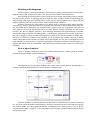
What integration with Excel gives ?
Power system studying practice in many facilities shows, that Microsoft Excel is widely used by
engineering stuff, especially for preparing data and reports generation. Spreadsheets abilities for calculation automation and data presentation are suitable for large amount of tabular data, which is usual for
power system studying. From the Excel’s user point of view – InorXL is add-in that enables to enter data
to Excel worksheets and to calculate load flow. Calculation results are placed to specific columns of the
same worksheets. All Excel features on sorting, filtering, additional calculation and chart representation
of data are still available. InorXL user interface is integrated to Excel as additional toolbar ribbon and
special taskbar. The last one allows to present calculation logs and convergence results. InorXL does not
alter usual Excel workflow. After InorXL installed it is possible to use all Excel functionality without any
limitations.
Being an add-in, InorXL is a part of Excel at runtime. All functions of InorXL available from user
interface are also available from Excel’s VBA environment. You can develop your own macros that utilize
load flow calculations. As you probably know, Excel offers ability to record user macros and to debug
them. Access to workbook data from macro language is simple and convenient, and possibilities to manage and analyze data are almost unlimited. So, macro development is not such hard deal, and it can save
huge amount of time.
All source and result data are stored in Excel workbook. There is no need in additional files and
databases. You can analyze your data and prepare reports even without InorXL installation, because
there is no any InorXL specific data in workbook. It makes sharing and publication of data very simple.
InorXL can import rg2 files – format of most widely spread in Russia network analysis software.
All necessary data can be transferred and converted to Excel workbook. Strictly speaking, there is no
InorXL file format, because it is regular Excel workbook with set of worksheets and formatted columns.
Thus, it’s not hard to import InorXL case from Excel.
What is system requirements ?
You can install and run InorXL on any computer that meets following requirements:
•
•
•
1
cal.
CPU is SSE3-enabled (virtually all CPUs manufactured from 2005).
Microsoft Windows XP/Vista/7 32- or 64-bit is installed.
Microsoft Excel 2007 32-bit or Microsoft Excel 2010 1 32- or 64-bit is installed. In 64-bit
operating system InorXL can run only as Excel 2010 add-in.
Excel 2010 is preferable, due to performance advantages on data loading and updating. But performance differences are not criti-
5
•
•
.NET Framework 4.0 is installed. .NET Framework is Microsoft system package required
to run .NET-application. Most of modern computers running Windows have this package
already installed. But if it is not, you can download and install this package from Microsoft site for free. The easiest way to find download area is to google it, for example,
with query “.NET Framework 4.0 site:microsoft.com”.
To read manuals and examples description you should install Adobe Reader or equivalent PDF viewer.
To import rg2-files any version of RastrWin software must be installed. If it is not, InorXL will be
still fully functional, except of importing cases in rg2 format. It is not possible to run RastrWin as automation object in 64-bit environment, thus rg2 import on 64-bit operation system is not supported.
InorXL is installed and configured by special installer program. Installer tests all system requirements and will not continue if any of them are not met. Installer requires user right elevation to administrator level, to write system files and folders. You may be asked for administrator rights by UAC
prompt.
How to install InorXL ?
To install InorXL run installer program InorXLSetup.exe. Installer will determine bitness (32 or 64
bit version) of operating system and Microsoft Office and install proper version automatically. Installer
may ask you for rights elevation (as most of installers, running on Windows 7/Vista does). To enable elevation just confirm UAC prompt. If your user account is not member of Administrator group, you may be
asked for Administrator password.
After startup, installer will present you license agreement. You must agree with it and then installer will begin to test your computer for system requirements. This test may continue up to half of
minute, depending on your computer performance. When test will be complete, the list of system requirements will be presented with green or
red checkmarks on each item. All items, except “RastrWin DB engine” must be green.
If all mandatory system requirements are met, proceed to install. All necessary components will be copied and registered on your computer. Two dynamic link
libraries will be installed to your Program
files InorXL subfolder, and few folders with
manuals, resources, and examples. There is
no own shortcut at desktop or Start menu
for InorXL, because it launches only when
Excel launches. To check InorXL is installed
properly, run Excel and ensure InorXL tab is
appeared on main Excel ribbon, and Taskbar
“Calculation results” is shown at the right of
worksheet area.
InorXL can be uninstalled from Control panel. Enter “Programs and components”, find “InorXL”
from list of installed programs, check it and click “Uninstall” at window title.
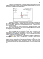
How to use InorXL ?
To begin your work just launch Excel. InorXL user interface can be found on main Excel ribbon in
“InorXL” tab. There are four buttons on the ribbon: “New”, “Import”, “LF” and “Help”. You can start new
case, load present case stored in xlsx format, or import rg2 file in “RastrWin” format.
InorXL workflow is as simple as possible. There are five worksheets with special formatting and
column sets. You can enter data to these worksheets and run load flow calculation. In case of successful
6
calculation worksheets will be filled with results. The shortest way to study InorXL is to take a look at
worksheet descriptions:
“Buses” worksheet
This worksheet presents buses (or nodes) descriptions of network model.
N
Bus identificator: integer positive number. It must be unique through “Buses” worksheets. If duplicates are found at start of load flow calculation, error message will be given.
Название Bus name. Any string you want. Name can be empty, but it is recommended to fill name
to make buses description clearer and to make branch names (see “Branches” worksheets below) more informative.
State
Can be selected from the list of possible bus states:
• Off – bus is switched off and grounded (voltage is zero);
• Slack – slack bus. Voltage magnitude and phasor angle are fixed;
• Load – load bus (PQ bus)
• Gen – generator bus with fixed voltage magnitude with reactive power within reactive power constraints;
• Gen+ –generator bus with fixed voltage magnitude and with reactive power limited by Qmax constraint;
• Gen- – generator bus with fixed voltage magnitude and with reactive power limited by Qmin constraint
While entering data you can select types Off, Slack and Load from combo-boxes. While
load flow calculation the rest of types will be determined automatically.
Unom
Nominal bus voltage magnitude measured in kV. It is mostly used for flat start and for
calculation of relative voltage values.
G
Real part of ground conductance. Positive number means active power consumption.
B
Imaginary part of ground conductance. Positive number means reactive power consumption (inductance shunt). Negative – means reactive power generation (capacitance
shunt).
Area
Area number, which bus belongs to. Areas are used to group buses for aggregation purposes into “Areas” worksheet. It is not mandatory field, if you are not going to calculate
aggregated areas parameters.
LRC
Load response curve number. Can be empty. See “LRCc” worksheet chapter to learn more
about LRCs.
Pl
Active load power in MW. Negative number means generation.
Ql
Reactive load power. In MVar. Negative number means generation.
Plc
Calculated active load power in MW with respect to bus LRC. If no LRC given Plc will be
equal to Pl. This field will be filled automatically after load flow.
Qlc
Calculated reactive load power in MVar with respect to bus LRC. If no LRC given Qlc will
be equal to Ql. This field will be filled automatically after load flow.
Pg
Active power generation in MW. Negative number means load.
Qg
Reactive power generation in MVar. Negative number means load.
Qmin
Lower limit of reactive power in MVar for generation bus. This field is in effect only in
case of Vref field is given (see below).
Qmax
Upper limit of reactive power in MVar for generation bus. The value in this field must be
greater than Qmin for this bus. This field is in effect only in case of Vref field is given (see
below).
Vref
Reference voltage magnitude for generation bus in kV. Load flow algorithm will try to enforce this magnitude while calculation. If this field is empty, voltage magnitude will be
calculated. To enforce voltage magnitude you have to give some range Qmax > Qmin for
this bus.
7
V
D
Calculated voltage magnitude in kV.
Calculated voltage angle in electrical degrees.
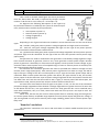
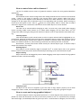
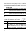
Take a look at network model figure and check parameters
from the above table. Bus load is expressed by Plc+jQlc complex
number. If LRC for bus is not in effect, Plc = Pl and Qlc = Ql.
For beginners the following descriptions on bus types may
be presented. Network is modeled by the system of nonlinear equations, which accounts each bus by four parameters:
•
•
•
•
types:
Active power injection 1 P;
Reactive power injection Q;
Voltage magnitude V;
Voltage angle 𝛿.
Depending on set of given and unknown variables in source data each bus can have one of three
PQ – load bus, with given power injections. Voltage magnitude and angle must be calculated.
V𝛿 – slack bus, with given voltage magnitude and angle. For this type of bus power injection
must be calculated to balance whole network island.
PV – generation bus with given power injection and voltage magnitude. Reactive power injection
and phasor angle must be calculated. For this type of bus one must also provide reactive power range
[Qmin;Qmax].
PV-type buses are used to model buses with generators controlled by voltage regulators. Regulator controls excitation of generator, which in turn, varies generator reactive power output. Reactive
power of generator is limited by its construction and regulator cannot provide constant voltage at generator bus when reactive power is out of acceptable range. If limits on reactive power are violated, voltage at generator bus becomes variable.
For load flow case calculation generator bus must be provided with reference voltage Vref and
reactive power range [Qmin;Qmax]. Until reactive power of generator bus within its range, bus will be
kept as PV-type. Voltage of this bus V will be equal to Vref, 𝛿 angle and reactive power output will be
calculated. When reactive power becomes greater than Qmax, bus type switches to PQ, and reactive
power output of this bus becomes equal to Qmax. Voltage magnitude of this bus becomes variable and
can differ from Vref. Such bus will be marked as Gen+. Again, if reactive power falls below Qmin, bus
type switches to PQ, reactive power fixes at Qmin and bus will be marked as Gen-.
For buses that were switched from PV-type to PQ (Gen+ or Gen-) to the rest of the calculation
procedure voltage magnitude will be checked. If voltage magnitude rises greater that Vref for Gen+ bus
or falls below Vref for Gen-, bus type switches back to PV. Each generator bus can be switched many
times while calculation, thus, as a result, some buses with Vref set may have V not equal to Vref. This
solution is feasible.
Please note, that the way we account reactive power limits is relatively rough, because generator reactive power delivery acceptable range depends on active power output and generator voltage. If
you are interested in more precise reactive power range modeling, please refer to reactive power capability curve 2.
“Branches” worksheet
The “Branches” worksheet is for source and result data on network model branches (lines) and
transformers.
Nhead
Head bus indentifier
1
2
Injection is difference between generation and load values.
Computational Methods for Large Sparse Power Systems Analysis. S.A. Soman, S.A. Khaparde, Shubha Pandit, 2001
8
Ntail
Nparr
Tail bus identifier
Number of parallel line to identify unique branch. Can be zero for single branch between
head and tail buses.
Name
Branch name. This field is filled automatically with respect to names of head and tail buses.
State
State of branch. Can be “on” and “off”.
R
Real part of branch resistance in Ohms. Can be zero.
X
Imaginary part of branch resistance in Ohms. Can be zero or negative.
G
Real part of ground conductance in 𝝁Sm. Positive number means active power consumption.
B
Imaginary part of ground conductance in 𝝁Sm. Negative number means reactive power
generation (conductance shunt), positive – reactive power consumption (inductance
shunt).
Ghead
Auxiliary real part conductance at the head of branch in 𝝁Sm.
Bhead
Auxiliary imaginary part of conductance at the head of branch in 𝝁Sm.
Gtail
Auxiliary real part conductance at the tail of branch in 𝝁Sm.
Btail
Auxiliary imaginary part of conductance at the tail of branch in 𝝁Sm.
Kt
Real part of transformer ratio. Ratio is defined as result of division of voltage magnitude
at tail bus of the branch by voltage magnitude at head bus. If Kt is zero or empty, InorXL
will treat it as unity.
iKт
Imaginary part of transformer ratio. It is ratio, not angle shift between voltage phasors !
Phead
Calculated active power flow at head of branch in MW.
Qhead
Calculated reactive power flow at head of branch in MVar.
Ptail
Calculated active power flow at tail of branch in MW.
Qtail
Calculated active power flow at tail of branch in MVar.
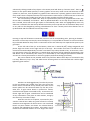
Depending on transformer ratio, branch model can be represented as power transmission line
model or power transformer model.
For Kt = 1:
For Kt ≠ 1:
9
Difference is in the way of shunt part modeling. Ordinary branch with Kt=1 has shunt conductance divided equally between head and tail buses. Transformer branch with Kt≠1 has whole shunt conductance at head bus.
Auxiliary conductances are introduced for compatibility with “RastrWin” branch model. These
conductances refers to “RastrWin” line reactors. Each reactor has conductance 𝐺0 + 𝑗𝐵0 . After importing load flow case from “RastrWin” Ghead, Bhead, Gtail and Btail will be filled with equivalent values
referred to line reactors: 𝑛(𝐺0 + 𝑗𝐵0 ). If your case created with InorXL these conductances may be ignored.
Branch may have zero or negative reactances. In theory, negative reactances leads to convergence problems, but in most cases InorXL can take workarounds with such parameters.
When load flow calculation is successfully completed, Phead, Qhead, Ptail and Qtail columns will
be filled with calculated power flows. Power flows are calculated at points “just near” bus connection, as
shown by metering transformers symbols at figure above.
Resistance of transformer branches refers to head bus voltage. Shunt conductance 𝐺𝑡𝑎𝑖𝑙 + 𝑗𝐵𝑡𝑎𝑖𝑙
refers to tail bus and will not be modified with respect to voltage magnitude.
“LRCs” worksheet
N
Load response curve identifier. When this number is entered to LRC field of some bus,
bus load will be controlled by this LRC.
Vmin
Voltage magnitude, from which the next piece of LRC has effect. See below for details.
P0
Constant power coefficient on active power.
P1
Constant current coefficient on active power.
P2
Constant impedance coefficient on active power.
Q0
Constant power coefficient on reactive power.
Q1
Constant current coefficient on reactive power.
Q2
Constant impedance coefficient on reactive power.
Active and reactive power loads can be modeled as functions of bus voltages. Usually load is expressed as 𝑃𝑙 = 𝑐𝑜𝑛𝑠𝑡, 𝑄𝑙 = 𝑐𝑜𝑛𝑠𝑡, but for some load types, such as electrical machines power consumption varies with voltage at its connection bus. Thus composite load model should be expressed as
𝑃𝑙 = 𝑓(𝑉), 𝑄𝑙 = 𝑓(𝑉), where 𝑓(𝑉) is expressed as polynomial:
𝑃𝑙𝑐 = 𝑃𝑙 �𝑃0 + 𝑃1 �
where:
𝑃𝑙𝑐 , 𝑄𝑙𝑐
𝑃н , 𝑄н
𝑉
𝑉ном
–
–
–
–
𝑉 2
� + 𝑃2 �
� �
𝑉𝑛𝑜𝑚
𝑉𝑛𝑜𝑚
𝑄𝑙𝑐 = 𝑄𝑙 �𝑄0 + 𝑄1 �
𝑉
𝑉 2
� + 𝑄2 �
� �
𝑉𝑛𝑜𝑚
𝑉𝑛𝑜𝑚
𝑉
calculated active and reactive bus loads;
given active and reactive bus loads;
calculated voltage magnitude at bus;
nominal voltage magnitude at bus.
𝑃0 , 𝑃1 , 𝑃2 и 𝑄0 , 𝑄1 , 𝑄2 coefficients are chosen to fulfill 𝑃𝑙𝑐 = 𝑃𝑙 и 𝑄𝑙𝑐 = 𝑄𝑙 at 𝑉 = 𝑉𝑛𝑜𝑚 , from
where 𝑃0 + 𝑃1 + 𝑃2 = 1 and 𝑄0 + 𝑄1 + 𝑄2 = 1.
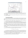
In some cases more than one polynomial required to model complex load response. Piece-wise
polynomials can be used for this purpose. Pieces are divided by Vmin parameter. As an example standard LRC of 3 pieces is given:
10
LRC on the figure on active and reactive loads is presented on the figure 1. Active power LRC is
modeled as single polynomial in �
𝑉
𝑉ном
� range from zero to infinity.
𝑉
𝑉 2
� + 0.47 �
� �
𝑃𝑙𝑐 = 𝑃𝑙 �0.83 − 0.3 �
𝑉𝑛𝑜𝑚
𝑉𝑛𝑜𝑚
Reactive power LRC has three pieces:
𝑉
𝑉
�
� < 0.815
,�
⎧0.657 + 0.158 �
𝑉𝑛𝑜𝑚
𝑉𝑛𝑜𝑚
⎪
⎪
𝑉
𝑉 2
𝑉
𝑄𝑙𝑐 = 𝑄𝑙 4.0 − 10.1 �
� + 6.2 �
� , 0.815 ≤ �
� ≤ 1.2
𝑉𝑛𝑜𝑚
𝑉𝑛𝑜𝑚
𝑉𝑛𝑜𝑚
⎨
⎪
𝑉
⎪1.708
� > 1.2
,�
⎩
𝑉𝑛𝑜𝑚
Both active and reactive power LRCs are described on “LRCs” worksheet in InorXL. The above
LRCs will be described as follows:
N
Vmin
P0
P1
P2
Q0
Q1
Q2
2
0.000
0.830
-0.300
0.470
0.657
0.158
0.000
2
0.815
0.000
0.000
0.000
4.900
-10.100
6.200
2
1.200
0.000
0.000
0.000
1.708
0.000
0.000
In this table Vmin separates pieces of LRCs. Active power LRC is in effect from Vmin=0 to infinity
and expressed by 3 coefficients. In the rest of table lines coefficients for this LRC are zero, despite of
Vmins are given. This means LRC on active power is not changed for these Vmins and will be in effect to
infinity with coefficients from first table line.
Reactive power LRC expressed by three different polynomials for each Vmin. While load flow calculation, load at bus referred to
this LRC will be controlled by these functions.
To control bus load by some LRC just enter LRC identificator
to “LRC” column on “Buses” worksheet. After load flow is calculated,
check values in columns “Plc” and “Qlc” and compare with “Pl” and
“Ql” values of the same bus.
Please note, that pieces of LRC must not have gaps by P or Q
at each Vmin points. An example of such unacceptable gap is shown
on figure. InorXL will check each LRC and inform user about found
1
This is standard LRC for 35 kV loads and it is referred as “Type 2” in Russian engineering practice.
11
gaps with error message.
“Areas” worksheet
N
Area number. If this number is entered to some node’s “Area” column, this node will be
included to this area.
Name
Area name.
Pl
Aggregated active power load in this area in MW.
Ql
Aggregated reactive power load in this area in MVar.
Pg
Aggregated active power generation in this area in MW.
Qg
Aggregated reactive power generation in this area in MVar.
dP
Active power losses in MW.
dQ
Reactive power losses in MVar.
Pcons
Active power consumption (Pl+dP) in MW.
Qcons
Reactive power consumption (Ql+dQ) in MVar.
The main purpose of areas to simplify analysis of power balances. Area aggregation allows to
present whole network in compact table. InorXL uses well known area setup, consisting of bus sets, referred to areas. To refer bus to some area just enter area number to “Area” column in “Buses” worksheet. Don’t forget to create area itself, by providing line with this number in “Areas” worksheet. After
load flow is calculated, “Area” worksheet will be filled with aggregated values. Values of Pl, Ql, Pg and
Qg are just sums of corresponding quantities of nodes, selected to areas. Area losses are sums of shunt
losses and branch losses. Because branch is not referred to area directly, it is assumed that the branch is
referred to the same area, to which head node is referred. Thus, all losses inducted by branch resistance
will be summed to head node area. This assumption is true both for lines and transformers.
If some bus is not referred to area, or area bus is referred to is not described in “Areas” worksheet, such bus will not be taken to any account.
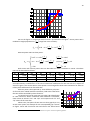
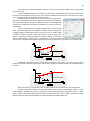
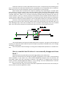
Let’s have a look at simple example
on IEEE-14 bus test system. Assume branches are directed from buses with greater
numbers. Buses 1 and 2 are referred to area
1 (blue). Buses 3 and 4 – to area 2 (yellow).
Load and generation power and power losses inducted by shunts will be summed for
corresponding areas. Branches 1-5, 1-2, 2-4,
2-3 and 2-5 referred to area 1 by its head
nodes and drops losses to area 1. Branches
3-4, 4-5 and transformers with heads at bus
4 drops losses to area 2.
Areas usage does not alter load flow result in any way.
“Parameters” worksheet
There are three parameters for InorXL. And all of them are parameters of computational module. “P imbalance” is acceptable imbalance on active power. Load flow solution will be considered as
feasible if imbalance on active power in any of buses is lower, than acceptable imbalance and reactive
power generation for PV buses will be in acceptable [Qmin;Qmax] ranges. By default P imbalance set to
1 MW.
“Iterations max” parameters limits iterative process to desired number of iterations of Newton
method. Startup method is not controlled by this parameter and may perform up to 100 iterations to
ensure initial guess quality. By default maximum number of iterations is limited to 20. If load flow case is
not calculated, you should consider imbalances at each iteration, presented by InorXL taskbar. If imbalance is continuously decreases, it may be a good idea to increase maximum iteration count and try to
12
solve load flow case again. Please note that imbalance curve may have peaks related to PV/PQ bus
switching. If imbalance increases continuously case may be inappropriate and should be revised. The
most common causes of bad convergence are high initial power imbalances, excessive amount of
branches with high R/X ratios, zero or negative impedances.
The “Flat start” parameter should be described in more details. Basic load flow solution method
is Newton method, which is iterative. To start solution, one should make initial guess about unknown
variables values. Newton method is known to be highly dependent on initial guess and may fail, if initial
guess is too far from point of solution. That’s why it is common practice to “prepare” guess for Newton
method by some more robust, but relatively slower solution method. In InorXL such preparation is provided by startup method (Seidell or Jacobi methods, depending on case and available CPU cores). But
even startup method may fail if initial guess is rough enough. For example, after load flow calculation
failure resulting variables may have inappropriate values. To prevent this, so-called flat start is used.
When flat start is in effect, all voltage magnitudes will be assumed to be equal to nominal voltage values
for load buses and reference voltages for generator buses. Phasor angles will be zeroed, except slack
buses, where phasors are given values. Reactive generation for generator buses will be set in the middle
of [Qmin;Qmax] ranges.
When calculating series of cases with small differences it may be useful to switch off flat start. It
will lead to faster calculation, because initial guess for iterative method is expected to be near solution.
Load flow should converge in 3-5 Newton’s iterations for cases with dimensions about 500 buses.
Startup method cannot be switched off, because solution reliability is much higher, and its computational costs are relatively small. For each load flow calculation InorXL performs at least one iteration
step of startup method even in case for which given imbalance is lower, than acceptable imbalance.
How InorXL interprets worksheets ?
Table structures presented above makes clearer to understand the way InorXL works with worksheets while load flow calculation. All worksheets are processed by the same way. InorXL requires following two simple rules to comply on each worksheet:
All required to interpret data columns must be presented on worksheet. Captions must be in the
first row of worksheet. The order of columns does not matter: you may change it and even hide (but not
delete) any of them.
Columns marked by black background in worksheets
descriptions (“Buses” – “N” for example), must not contain
empty cells until the end of worksheet. InorXL will read data
from the top to the bottom of worksheet until first empty cell.
In case of empty cell is found, InorXL will lock row count for this
worksheet and refuse to read any cells below first empty one.
Columns marked by black in worksheet descriptions are also
called key field columns. They are used to identify model objects and to determine effective sizes of worksheet.
When LF button is clicked, InorXL will check all necessary worksheets are in current workbook. InorXL will report
error in case of any required worksheet is not found. Then, effective sizes of each worksheet will be determined. And at the
end of source data preparation InorXL will read and check all
data. In case of any error on data format an error message will
be given.
When all data is successfully checked, InorXL will build
internal representation of network mode and will try to calculate load flow. After load flow is completed, InorXL will output
all results to the same worksheets. It must be pointed out, that
column order does not matter. And even if you change default
order, results should be output correctly.
13
You can use any of Excel tools to transform and present data. For example, you may sort and filter your data. Load flow will be performed correctly even when autofilter is active. This one is useful to
focus on important part of model. Of course, autofilter affects only data view: load flow will be performed always with whole unfiltered model.
How to use taskbar ?
When Excel starts, InorXL will add its toolbar to the main ribbon and create taskbar to the right
edge of Excel window. Taskbar helps you to inspect calculation process and to check possible error and
warning messages. Taskbar is dockable window. It may be detached from main workspace and behave
like independent window. You can close taskbar, but on the load flow command it will appear again.
There are two areas in the taskbar. The first area is calculation results list, second is a log. Areas are divided by splitter. You can move splitter to control each area size. If taskbar width is greater than height,
areas will be oriented horizontally, otherwise – vertically. At each load flow areas are cleared.
When iterative calculations are performed, some technical parameters appeared to the calculation result area. These parameters may be useful to identify and get rid of convergence problems.
N
Iteration number
P
Maximum error on active power in MW. This is infinite norm of P vector
Bus
Bus with maximum active power error
Q
Maximum error on reactive power in MVar
Bus
Bus with maximum reactive power error
MinV
Minimum voltage magnitude in KV
Bus
Bus with minimum voltage magnitude
MaxV
Maximum voltage magnitude in KV
Bus
Bus with maximum voltage magnitude
‖𝐈𝐦𝐛‖
Euclidean norm of composite PQ error vector
Errors can help to estimate iteration progress. Sequential decrease of errors shows good convergence. Errors may have peaks, related to PV/PQ bus type switching. Voltage magnitudes determine
solution quality. When voltage magnitude drops below 0.5 of Unom or raises greater than 2 of Unom,
calculation interrupts with error. Calculation module tries to keep voltage magnitudes in acceptable
ranges by ordered PV/PQ bus switching.
Startup method does not use ‖Imb‖ parameter, thus you may see “N/A” in this column for
startup iterations. Startup method iterations are shown in gray text and Newton method are in black
text.
Log area shows basically messages, warnings and errors. You can click message, and in most situations InorXL will show worksheet and object on which message was generated.
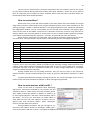
How to write macros with InorXL ?
InorXL can be used as component when developing
VBA macros. All functions available by user interface are also
available in VBA. To create macros you have to enable “Developer” ribbon of Excel. By default it is hidden. To enable it, go
to “Excel options/Popular” and check “Show developer tab on
the ribbon”. This way is for Excel 2007. To enable ribbon in
Excel 2010 click “File” tab, click “Options” and then in the categories pane click “Customize ribbon”. Select “Developer”
from list and click OK to close options.
Having enabled “Developer” tab you can begin to create macro. Click “Macro” button on “Developer” ribbon, give a
name to new macro and click “Create”. Visual Basic for Applications workspace will be shown.
14
To use InorXL functionality in VBA you have to make reference to its module. Go to the “Tools”
menu and select “References”. Select and check “InorXL 1.0 Type Library” from the available references
list and click OK.
Now you can use InorXL in VBA. References to InorXL are made through variable of type InorXLAddin.
Sub NewMacro()
Dim spInor As InorXLAddin
End Sub
Variable must be initialized by InorXL object reference:
Sub
Dim
Set
End
NewMacro()
spInor As InorXLAddin
spInor = Application.COMAddIns("InorXL.InorXLAddin.1").Object
Sub
When initialized, spInor variable will refer to InorXL instance loaded by Excel. You can check
availability of InorXL with following code:
Sub NewMacro()
Dim spInor As InorXLAddin
Set spInor = Application.COMAddIns("InorXL.InorXLAddin.1").Object
If Not spInor Is Nothing Then
' Make something using InorXL
Else
End If
MsgBox «InorXL is not installed»
End Sub
From the InorXLAddin LF (Load Flow) method is available:
InorNetStatus LF(FlatStart, SaveResults)
There are two parameters. FlatStart parameter forces flat start when non zero. SaveResult parameter enables to update results after calculation. You can disable update to speed up massive calculation when only solution feasibility is important. All parameters by default are True, so you can omit
them. Return values of LF method are of type InorNetStatus:
STATUS_OK
Calculated successfully
STATUS_ERROR
Calculation interrupted due to errors in source data
STATUS_UNKNOWN
Unknown error
STATUS_NOCONVERGENCE Calculation failed due to convergence
STATUS_VMAX
Calculation interrupted due to raise of voltage magnitude in some node
greater that two of nominal voltage
STATUS_VMIN
Calculation interrupted due to drop of voltage magnitude in some node
below that half of nominal voltage
STATUS_BRANCHDELTA
Calculation interrupted due to phasor angle difference of some branch
is greater than 90О.
Macro can be runned by «Run» button or by menu command «Run»/Run Sub
UserForm». Macros are stored in Excel only with special type of book with “macro support”.
Check type of workbook you saving, or your macros can be lost.
When workbook is loaded, Excel can disable macros due to security reasons. To enable macros
use “Security” button on “Developer” ribbon. To work without any limitations select “Enable all macros”. Please note, that security limitations will not be in effect, and you have to be careful when running
untrusted content.
15
Working with diagrams
Tabular network model representation is well suited for working on large amount of model data.
Engineers are familiar with this form but it is not the only form needed to work effectively.
One line diagram representation is more common view of model. Some details may be omitted,
but the attention focuses on topology and most important state variables. Almost all engineering software packages offer both forms simultaneously. InorXL also has special graphical tool to create, edit and
analyze network model. Later on this manual it will be called simply “Graphics”.
Graphics represents the same objects as in tabular views as visual primitives: buses, branches,
transformers, reactors, generators and so on. Graphical representation is almost independent from tabular. All model objects parameters are available both in tabular views and in graphical view. Data set
form graphics is even more detailed description of model, because it holds information not only on parameters, but also on diagram geometry. Data exchange between both representations is possible,
which makes diagram creation and editing easier. Data between representations is linked by bus numbers. Bus in diagram receives and sends its parameters to the bus with the same number in tabular view.
Branches are linked by its border buses numbers and by its parallel line number. This way of linking
makes permissible inexact matching of tabular views and diagram. You can put on the diagram part of
mode needed only, and conversely: supply for large diagram small part of tabular model description. So,
diagram and tabular views are independent, but linked only by the bus numbers, were set in both representations.
How to open Graphics ?
There is “Graphics” button on InorXL tool ribbon. When pressed, it opens graphical window,
containing all tools needed to work with diagram.
The largest area in this window is diagram view. There is also context panel on the right side. Its
content and tool set are dependent on current selection in diagram view.
Graphical window is a child window of Excel. When Excel is minimized, this window is minimized
too. There are standard window control buttons: minimize, maximize and close in the title bar of graphical window. When user closes graphical window, it disappears from desktop, but it is not to be destroyed actually. When “Graphics” on the tool ribbon is pressed again, graphical window will be shown
in its previous state.
16
How to control view and its elements ?
The set of available control actions of graphical window is similar for most graphical Windows
applications:
Scale view
Mouse wheel can be used to change view scale. Rolling towards the user zooms out and towards
screen – zooms in. The origin of zooming is the current mouse cursor position. When [Ctrl] key is
pressed, any part of the diagram can be selected by dotted frame. When selection is done, scale will be
changed to fit the largest side of selection frame to corresponding side of window. When zooming by
frame cursor will appear as lens. There is
button on context panel, which is shown when no object
selected in diagram view. This button scales view to fit all visible objects in current window.
Move view
The view can be moved without changing its scale. To move view, press [Shift] while dragging
mouse. Pressing middle mouse button (or its wheel) while dragging, has the same effect. You can
change scale while moving by rolling mouse wheel too. Mouse cursor is represented as hand while moving.
Selecting objects
Click desired object by left mouse button to select it. Object selected will be highlighted by cornered frame. Selection includes object itself and all its dependent objects. Some types of objects cannot
be selected independently, because these objects are children of another object. Transformers, for example, are children of buses. So, when selecting transformer the whole parent bus is selected.
Nevertheless, context panel shows toolset exactly for selected object type. To deselect object
simply click outside of any object.
Rotating objects
Most objects can be rotated by angle of multiple of 90о. To rotate object click on the rotation
button (small circled arrow) shown above selected object. Rotating cycles counterclockwise by 90о.
Objects moving
Object selected can be dragged by mouse. When dragging some object outside of the graphical
window the view is moved accordingly.
Snapping to grid
All objects in the view are snapped to grid. This helps to align objects properly and to draw
straight lines. Grid is visible, until selected object is moved. When moving stops, grid goes off again.
How to create and set up graphical objects ?
The whole diagram consists of graphical primitives. To create diagram these primitives must be
placed into view and connected. The one of most basic primitive is bus. It is represented by rectangle
with fixed height, and width dependent of given bays count. To add new bus to diagram, first cancel any
17
selection by clicking outside of any objects. The context panel will show up “Common view”. There is
button on this panel. When pressed, it enters graphics to bus entry mode. Cursor will be shown as bus
symbol. To place bus, click anywhere in graphical view. When bus is placed, graphics returns from bus
entry mode. There is keyboard shortcut for bus placement: Home button. It places new bus at center of
view. To cancel bus entry mode press [Esc] key or select another tool from context panel.
Bus can have bays on both sides. They are represented by short lines, perpendicular to bus. One
of bus sides is called Red, and another – Blue. By default Red side is on the top of bus primitive. When
bus is rotated, these color marks give option to still indentify sides. Sides are highlighted by color only
when bus is selected. The new bus by default has one bay on the top and one on the bottom. Bays count
on any side can be changed by pressing colored buttons at “Bus” context panel. These buttons acts as
up-down dials and also indicates current bays count:
Pressing on top half of button increases bay count on side of corresponding color, pressing on bottom –
decreases. If some bays are busy by connected objects, it is not possible to decrease its count until these
bays released. Maximum bays count is restricted to 16 for each side. Bays are separated in space by two
grid steps.
At the left side of bus (or at the bottom, when bus is rotated by 90о) voltage magnitude and
phasor angle are shown. At the right side (or at the top) – bus number and name. Text blocks can be
moved and rotated independently from bus. Text blocks stays always linked to bus, so when bus is moving, text blocks moves too. When bus is rotated these text blocks will be realigned automatically. Also
text blocks can be rounded by thin frames, as it demanded by some diagram presentation standards.
You can turn frames presentation on and off in graphics preferences dialog (see below).
Bay can be found on two possible states: busy and free. When some object is connected to bay
it is busy. When not, bay is free, and while mouse hovering above its unconnected end it will be highlighted by green marker:
Markers can be dragged away from bus by mouse.
In this case branch will “pulled” from bay. One end of this
branch will be connected to bay already. The other end of
branch pulled can be connected with any free bay of another bus. If right mouse button is pressed on marker,
transformer will appear connected to bay. To remove transformer right click it again. Transformers can be considered
as bay continuation. They have its own markers, acting by
the same way as markers of bays.
Branches are the set of points, connected by horizontal or vertical lines. When any point of branch is moved,
automatic rearrangement of all lines occurs. For unselected
branch no point markers are shown. For selected branch,
all points will highlighted by markers. All markers can be
moved. Start and end markers are a bit larger than other.
18
These markers can be “glued” to bay markers, connecting branch to bay. To disconnect branch, select it
and drag start or end marker away from bay. Bay will be freed. Branch has two text blocks, connected to
start and end markers to show power flow values. Also branch has arrows, showing direction of the flow
through it. For unconnected branch flow will be shown as “#” symbol. Text blocks can be moved and
rotated independently from branch. When branch state is off, it will be shown by dotted line.
Bus and branch selected can be deleted by pressing [Del] key. On bus deletion all branches have
been connected to it will be disconnected, but not removed from diagram.
How to set up model parameters using diagram ?
All parameters of object in diagram can be split up on two groups. The first group is for geometry, view mode and interconnection of objects. Second group consists of model parameters, which are
connected to tabular model data in Excel. For selected object parameter set will be shown in context
panel. Buses, branches, transformers, generators, reactors and compensators have its individual context
panel. So graphics can not only create and view diagrams, but also makes possible to create full model
data set.
Users can choose appropriate way for model creation. If one has tabular data, graphics helps to
create diagram easily, by reusing tabular data. After successful load flow all parameter values will be
transferred to diagram and shown on it. If user has no tabular data, it can be easier to draw diagram
with graphics, supplying model data by accessing graphical objects properties.
Beta versions have diagram-table transfer temporarily disabled
Consider example of use context panel for bus. To access panel select some bus in diagram.
The whole parameter set is shown on panel. One can enter load power values:
19
and then, power of generation at bus:
then, reactor conductance value for inductive compensation
or capacitive compensation
20
As you can see graphical representation of bus reflects parameters entered with context panel.
In addition, any connected to bus object can be edited individually. At the picture below there is generator context panel, available for selected generator object.
All tabular data is transferred to diagram on each load flow calculation. Also all parameters can
also be edited in tabular representation. You can see calculated load flows on branches and voltages at
bus at the pictures above. Please note, that all texts have white contours around, to clarify representation in case of object overlays.
Generator, reactor and load primitives are placed at bus automatically. Text blocks can be
placed manually, but after bus rotation text blocks will be rearranged again. Bus moving does not cause
any rearrangements of bus dependent objects.
How to use common view tools at context panel ?
Common view available when there is no selection on diagram. Common view tools are for operations with whole diagram. The most useful operation is probably bus search. To find bus, enter its
number at field and press
or [Enter] key. Diagram will be zoomed at bus found. If bus with given
number is not found, search text box will be colored in red.
Using common view it is possible to save current diagram or load file with saved diagram by
pressing
/
or
buttons. Diagram is saved in XML format. All information on geometry, connections and parameters is saved in this file.
Diagram can be printed by pressing
button. Print setup is available with
button. It opens
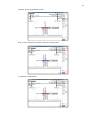
dialog, where you can choose printer and set its options, and also set up page split for large diagrams.
Paper size selected for current printer and its orientation are used to set up page splitting. You can set
pages count in horizontal and vertical directions. When checkbox “Show split” is marked, diagram shows
lines, representing page borders. The picture below shows split on four landscape oriented pages of A4
size.
21
Non-printable area is grayed out. In page split view mode it is also possible to move and zoom
diagram, to fit it to printable area manually. As size of graphical window changes page borders rearranges accordingly.
The preferences
button brings up preferences dialog, where bus voltage and name framing
can be turned on and off.
Continuation load flow
The “Continuation load flow” term means directed load flow parameters change in the way that
leads load flow to unstable or infeasible state. Stability margin detection and acceptable state variable
values screening with continuation load flow are basic tasks of power system engineers (in Russia, at
least).
Load flow which is close to stability margin is called “border state”. This state is described by
fixed values of state variable: power flows, currents, voltage magnitudes and so on.
There are no automatic methods for stability margin detection. System engineer has to isolate
vector of independent state variables, give it some direction and begin to change them accordingly, until
load flow became infeasible. Values of vector components fixed just before infeasibility will describe
border state.
Parameters vector with given laws of its components changing is called “trajectory”. Any border
state is linked with its trajectory, it found by. Trajectory may also contain some variables, which values
are tracked. Usually law of changing of independent parameters is linear: from initial value 𝑉𝑏𝑒𝑔 , to the
end value 𝑉𝑒𝑛𝑑 . Value of 𝑉𝑏𝑒𝑔 in most cases is chosen equal to initial case, but can be set to any value of
engineer choice.
Term “trajectory point” – 𝑡 often used to simplify trajectory control. Value of 𝑡 can vary in range
between 0 and 1. Thus, change law of trajectory component 𝑉 𝑖 can be written as:
𝑖
𝑖
𝑖
+ 𝑡 ∙ (𝑉𝑒𝑛𝑑
− 𝑉𝑏𝑒𝑔
)
𝑉 𝑖 (𝑡) = 𝑉𝑏𝑒𝑔
So, continuation load flow by given trajectory turns to successive increasing of 𝑡 with some step
and load flow solution at each trajectory point. System constraints and load flow feasibility must be
checked while trajectory following. Continuation load flow will result in border state, with some value
𝑡𝑙𝑖𝑚 and values 𝑉 𝑖 (𝑡𝑙𝑖𝑚 ). If border state is not reached, trajectory has insufficient length and it must be
increased (for example, 𝑡 should grow over 1, or 𝑉𝑒𝑛𝑑 should be increased).
Successive increasing of 𝑡 is called trajectory following. Please note, that for 𝑡 = 0 load flow
must be feasible and no system constraints violation can be accepted.
22
Stability margin can also be described indirectly by values of dependent variables, achieved by
load flow solution. To access its values during trajectory following so-called “tracked variables” are used.
For example, trajectory can control loads at some buses, and tracked variables can collect data on some
branch flows. Border state reached by this trajectory can be represented by border loads, and/or by
border flows. Often flows are used to describe margin of border state, because it is easier to collect
branch flows measurements in actual power system control.
It is common to distinguish border states by stability and by system constraints.
Border state by stability margin
Classical way to establish stability of power system for small disturbances requires its linearization and analysis of eigenvalues of state matrix. This is complex computational task, and often instead of
eigenvalues calculation it is possible to examine constant term of characteristic polynomial. Change of
its sign while trajectory following indicates crossing of stability margin. Further simplifications allows to
associate constant term of characteristic polynomial with the Jacobian. The list of assumptions, which
makes this association possible, is:
1) All generators in small disturbances model are represented by PV-type buses in load flow model.
2) All loads in small disturbances model have the same linear response curves in load flow model.
3) Infinite power bus in small disturbances model matches slack/swing bus in load flow model.
Thus when following trajectory from feasible state at some point Jacobian changes its sign, this
point is beyond stability margin. As trajectory point closer to stability margin, load flow solution becomes more numerically unstable, because Jacobian tends to zero. So, the point where load flow starts
to diverge also considered belonging to unstable state.
Border state by system constraints
When load flow solution exists and it is feasible it is not guarantee that in real power system this
case can be performed. This is due to power equipment has specific constraints, limiting operation voltages, acceptable long term currents and so on. So for trajectory following it is necessary to check constraints and determine border state as close as possible to state, where one or many constraints becomes violated. Stability margin and margin induced by constraints does not match so when trajectory
following the first encountered margin will be set as border state margin. There is continuation load
flow mode for which constraints are checked, but not considered while border state margin search (see
chapter “Tracked variables and constraints set up”.
Continuation load flow in InorXL
To perform CPF special workspace provided in InorXL. To access it press CPF button on InorXL tool ribbon. There are three areas in
CPF workspace: toolbar, source data panel and resulting data panel.
CPF trajectory set up
Trajectory is represented by vector of independent variables. For each variable change law must
be provided. Also list of tracked variables and constraints set are part of trajectory data, in terms of InorXL. Source data panel of CPF workspace has two tabs: “Trajectory” and “Tracking”. First tab is for trajectory vector set up. Second is for tracked variable list and constraints set up.
Up to 16 independent variables can be set for one trajectory. For each variable there is special
lane in source panel. Lane consists of header and track. Header holds the name of variable and its model
linking attributes. Track is for variable change law setup. There is an action bar on action track. It can be
moved and sized with mouse along track. At the top of the trajectory tab special ruler is placed. The ruler is marked in CPF steps. Current step can be chosen by CPF cursor, by clicking on ruler. Vertical line,
crossing all lanes is linked with cursor. When some action bar is crossed by cursor, it is considered active
and colored in red. Active action bar injects value of variable calculated by given law into model data.
23
Lanes can be turned off (“muted”) or exclusively turned on (“soloed”). This can be achieved by
pressing corresponding buttons on header.
Muted lane will have no effect on model. Soloed lane will disable all other not soloed lanes. The
value of model variable for disabled lane is unchanged and matches initial case value.
Mouse wheel zooms lane view in or out. Zooming is performed relatively to CPF cursor position.
To assign lane to model variable (or in another words – link
lane with Excel’s data), double clink lane header. Model link properties for lane will be open.
Lane caption can be entered into “Caption” field. To access
model variable its object’s type, variable type and object’s key must
be selected. There are three list boxes for it. “Type” list box allows
object type choosing: bus, branch or area. In dependence of object
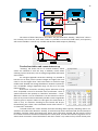
type “Parameter” list allows choosing variable type:
Type
Bus
Parameter
Units
Meaning
Pl
МW
Active bus load
Ql
МVar
Reactive bus load
Pl/Ql
МW/ МVar Conforming bus load (linked by initial case ratio)
Pg
МW
Active bus generation
Qg
МVar
Reactive bus generation
Pg/Qg
МW/ МVar Conforming bus generation
Vref
kV
Reference voltage magnitude for PV-bus
Angle
Degrees
Voltage phasor angle (meaningless for all buses, except slack)
Gsh
µSm
Active conductance at bus
Bsh
µSm
Reactive conductance at bus
Branch Kt
Real part of transformer ratio
iKt
Imaginary part of transformer ratio
Area
Pl
МW
Aggregated active area load
Ql
МVar
Aggregated reactive area load
Pl/Ql
МW/ МVar Conforming aggregated area load
And to finish assignment of lane the number of object must be selected from “Key” list. For buses and areas it is single number. For branches key is complex, and consists of three values: head bus
number, tail bus number and parallel line number, separated by commas. Key can be selected from list
or entered manually. When key entered is not found, list contents will be colored in red.
Lane caption are built automatically in the following format:
ObjectType[ObjectKey].ObjectParameter
Example:
Bus[28].Pn
Branch[37,9001,1].Kt
Area[3].Pl/Ql
24
Lane caption can also be entered manually. To return to automatic caption mode, simply clear
its field contents.
Linked variable will show up its caption on lane header. If parameter link is wrong, red circle will
be shown at lane header at first CPF step. This indicates problem in link that has to be corrected. In addition, warning message will be output to results panel.
Change law for variable can be set up by accessing action bar.
Bar itself can be adjusted by mouse within track. Double click on action
bar brings up parameter properties dialog. Controls of this dialog allow
setting up of change law and action bar behavior in relation to CPF cursor position.
There is mode switch in “Change method” frame. “None” mode
turns variable changing off. No changes in variable will occur despite of
variable properly linked and its lane is not muted. “Const” mode makes
variable to become constant value under cursor. Value of constant is
given in “Min/Const” field of properties dialog. In “Range” mode value
will be interpolated in range given by “Min/Const” and “Max” fields. Left side of action bar links to
“Min/Const”, and right side to “Max” field. Exact position of action bar also can be set in position fields.
“Maximum value beyond end” switch forces variable to keep “Max” value even in case cursor
position is beyond right side of action bar. This mode is useful to model constraints of independent parameters.
When this switch is off, variable value outside of action bar will match to value of initial case.
Variable interaction mode with model parameter can be set by corresponding switch. In “Set”
mode absolute variable value will be injected to model, replacing original parameter value. In “Add”
mode variable value will be summed with initial case parameter value. And in “Mult” mode these values
will be multiplied. The last mode allows to model non-linear variable change law.
25
The names of fields “Min/Const” and “Max” are just declarative. Actually, “Min/Const” value is
not necessary has to be less, than “Max” value. It is possible to reverse this field values, and trajectory
will control variable in reverse way: variable will decrease while trajectory following.
Tracked variables and constraints set up
“Tracking” tab shows the list of tracked variables, whose
values are collected at each CPF step. In addition, InorXL allows
checking system constraints, such as voltage magnitudes and branch
overcurrents.
For voltage magnitude constraints checking it is possible to
limit bus set to those, which nominal voltages are higher than indicated in “For bus higher than” field. This feature is useful for large
models with detailed low voltage distribution networks representation. Acceptable voltage magnitude range can be set in the next
field in percent.
Overcurrent constraints checking require indication of long
term acceptable current for branches and transformers. There is
special column for this quantity on “Branches” worksheet – “Imax”.
When this column is not on worksheet it can be created as usual in
place of any unused column. Maximum possible current magnitudes
must be given in amperes. When no value given for some branch or
value is zero, no constraint checking for this branch will be performed during CPF. There is also calculated current value column “I”
on “Branches” worksheet.
“Consider while CPF” switch enables constraint checking while trajectory following and its consideration in border state detection. Actually, at each CPF step InorXL calculates load flow and checks its
feasibility, and then checks constraints given. When some constraints violated and this switch is off the
list of these constraints violation will be output to result panel, and CPF will continue. Engineers can examine these constraints in Excel worksheets. But when switch is on, InorXL will try to find closest possi-
26
ble solution to the point, where constraints become violated. In this mode output of load flow results
with violations to Excel worksheets is disabled.
All tools needed to control tracked variables are located at “Tracking” tab. The list of tracked
variables is similar to file list of Windows explorer. List items can be selected by one and by group. Each
tracked variable is linked to model in the same way, as independent trajectory variable. Items in list represented by light bulbs icons, of three possible types:
–
–
–
Tracked variable linked to model properly, active and ready to collect data
Tracked variable inactive. Data will not be collected for this variable
Tracked variable is not connected to model properly. Data will not be collected for this variable. Link to model has to be corrected
The toolbar above tracked variables list is to control it:
–
Add new tracked variable. This button brings up variable properties dialog, which allows to
link it to model
– Remove selected variables. This button active only when at least one variable is selected
– Edit selected tracked variable. This button is active when exactly one variable is selected. It
brings up variable properties dialog. This dialog can also be accessed by double click on
some variable
– Activate selected variables. This button is active only when at least one variable is selected
– Deactivate selected variables. This button is active only when at least one variable is selected
– Clear collected data for all tracked variables
Tracked variable properties dialog is almost identical to trajectory parameter dialog. The only
difference is types of parameters available:
Type Parameter
Unit
Meaning
Bus
Pl
MW
Active bus load
Ql
MVar
Reactive bus load
Pg
MW
Active bus generation
Qg
MVar
Reactive bus generation
Angle
Degrees
Voltage phasor angle
V
kV
Voltage magnitude
Branch Phead
MW
Active load flow at branch head
Qhead
MVar
Reactive load flow at branch head
Ptail
MW
Active load flow at branch tail
Qtail
MVar
Reactive load flow at branch head
I
А
Branch current
Area
Pl
MW
Aggregated active area load
Ql
MVar
Aggregated reactive area load
CPF results and its analysis
The main CPF result is border state, achieved by following CPF trajectory, depending on cause of
following termination (LF divergence or constraint violation). When border state caused by stability
margin crossing the case found usually moved by trajectory back, for security reasons. This is due to fact
that even small disturbance of case close to stability margin can push system to instability. It is common
to set two margins for practical power system dispatch. The first one is closer to stability margin and
called emergency margin. The distance from stability margin usually 8% of load flow in border state. The
second margin called operational, with distance 20% of the flow in border state. In addition voltage
magnitudes are secured on level above 15% of border state. When border caused by constraints violation, it is used as is with zero security distance.
Engineers are often interested not only in border variables values, but in dependencies between
system parameters. CPF can reveal these dependencies and help to identify many sorts of problems in
power system. CPF provides variable tracking both in tabular and graphical forms.
27
CPF workspace has result area with CPF log and two tabs: “Track chart” and “Track table”. CPF
log receives information on current CPF step and violated constraints. “Track chart” tab holds chart control, able to show tracked variables for each step graphically against step position. On “Track table” tab
the same data is available in tabular form. At any moment both chart and table can be cleared by pressing button. Chart control supports clipboard copying in graphical (Windows metafile) and tabular (csv)
formats. Tabular form is suitable for pasting into Excel worksheets, which opens possibilities for additional results processing with Excel tools and charting system.
Chart control operation
To view tracked variables graphically special chart control is provided. It can present many variables simultaneously with separate channels. Chart control window can be controlled by mouse.
Drag
Show coordinate axis as dotted lines, crossed at cursor. For each axis tooltips
are shown with numerical values. Axis cross can be moved while holding
mouse button. If multi-axis mode (see below) activated, y-tooltip shows coordinates for active y-axis. To activate another axis click on it. Active axis is highlighted by red shadow
[Ctrl] + Left click
Zoom chart by 50%
[Ctrl] + Drag
Enter zooming mode. Mouser cursor drags zoom frame corner. When mouse
button released, chart windows zooms framed part of window. Previous zoom
and pan are stored
[Ctrl] + Right click
Return to previous zoom and pan. If nothing stored, zoom out by 50%
[Shift] + Drag
Enter pan mode. Cursor will appear as hand. Move mouse to pan chart window
Mouse wheel
Zoom in/out relatively to chart window center
When hovering cursor above some channel tool tip will appear soon indicating
channel legend. Right click on channel shows context menu for this channel. Right
click outside any channel show context menu for common chart properties.
Menu contents are different but contains some identical items referred to
common chart properties.
Show all
Grid
Legend
Print
Copy
Recalculate scale to fit all channels to current window frame
Toggle grid view
Toggle legend view
Select printer and print current chart view
Copies chart contents to clipboard. There are three possible copy modes, available for
choice in submenu: “Image”, “Data”, “Data+Time”. In image mode graphical content
of the window will be copied in WMF format, suitable for most windows applications.
In data mode table with numerical values for each channel will be copied in csv format. Data+Time mode is identical to data mode, except table will contain additional
column with CPF step values, to which channel points refers. Table header in Data and
Data+Time modes depends on switches in “Captions” submenu. When checked, table
header will contain column captions, formatted from legends of channels.
On the right side of chart window there is a list of channels captions – legend list. When cursor is
hovering above some legend item it will appear as pointing hand. Left mouse click brings up channel
properties dialog. If legend list does not fit to chart window height, scroll bar will appear at the right side
of list.
28
Any changes in channel properties dialog reflects in chart window immediately.
Caption
Marker
Width
Line type
Color
Chart type
Axis
Sort
Caption of channel, used to show legend. You can enter any desired string
Allows choosing marker type from the list: “Circle”, “Square”, “Right”, “Down”, “Left”,
“Up” or “Diamond”. It is possible to turn markers off. When viewing curves with many
points no-marker mode can substantially speed up chart drawing
Allows setting channel line width in range 1-10. Curves of width greater than 1 can be
only shown as solid lines
Allows choosing line type «Solid», «Dashed», «Dotted», «Dotted-dashed», «Dotteddouble-dashed». Curves of width greater than 1 can only be shown as solid lines
Allows selecting channel color with standard color picker control
Allows choosing of channel drawing mode «Curve», «Ladder», «Histogram». In Curve
mode channel is shown as is point-by-point. Ladder mode represents channel by orthogonal lines, connecting neighboring points. In Histogram mode drawing is the
same, as in Ladder mode, but rectangles, based on orthogonal lines and standing on xaxis are filled by solid colors.
Curve mode is well optimized to show curves with multitude of points. Other modes
can be slow with such large curves.
Allows choosing special y-axis for channel. This mode also called multi-axis. List contains numbers, corresponding to channels in current chart. Choosing any number it is
possible to create new y-axis (if no axis for this channel already), or refer channel to
existing y-axis. All axes have individual vertical scales which allow fitting many channels even with very different values. By default all channels refers to axis with number
0. When there are many axis in chart window one of them is always active and highlighted by red shadow. To make desired axis active simply click it. Active y-axis is used
to show y-tooltips when dragging measurement cross within chart window.
When checked, all points of channel are automatically arranged by its x-values. When
unchecked original order on x-axis is restored. CPF sends channel data sorted already.
CPF control
CPF workspace user interface allows choosing of any point on CPF ruler by moving CPF cursor
with mouse. When cursor is moved and released at some point, in one second command will be transferred to InorXL LF module and CPF step performed. CPF step consists of load flow solution and constraints checking. CPF step results will be shown in results panel. If some tracked variables are set, data
on them will be shown in chart and tabular views. Load flow results also will be transferred to Excel
worksheet. This CPF mode is known as “manual”.
There is also automatic mode, available from CPF workspace toolbar:
–
–
Run CPF trajectory following from current cursor position until trajectory end (last action
bar end) or until border state detection
Run CPF trajectory following from the first point of trajectory
29
Automatic mode CPF can take substantial amount of time. To stop CPF trajectory following press
[Esc]. In automatic CPF mode Excel worksheets are not updated, to save computation time. Tracked variable values are sent to chart and tabular view for each CPF step as in manual mode.
When border state encountered CPF trajectory following stops. Depending on “Consider while
CPF” switch on “Tracking” tab CPF will or will not consider system constraints. When border state is
forced by stability margin crossing, InorXL will refine this margin with step division technique. In case
“Consider while CPF” switch is on, and InorXL encounters feasible load flow solution, but with constraints violation, it will try to step by trajectory back and find closest possible load flow without constraints violation. When switch is off, information on violated constraints will be output to results panel.
These results are ranged by violation hardness. The first 10 hardest violations are screened at each step.
Until CPF is not encountered border state, it will follow by trajectory with unity ruler step. So,
the longer action bars the finer actual step. When border state encountered, CPF steps back and try to
make half-length step. If new state is feasible, CPF tries to continue with half step, if no, step is divided
again. This cyclic process repeats until step become lower than 0.01 at last feasible state point.
This method requires at least one feasible state point in trajectory. This point is the first point of
trajectory for automatic modes. When first point of trajectory represents infeasible state, error message
will appear in result panel.
Also result panel receives messages on wrong links of independent parameters or tracked variables.
How to reenable InorXL when it is occasionally disappeared from
Excel ?
Microsoft Excel has special ability to prevent buggy addins, that crashes Excel.
When you launch Excel, the message may appear, saying about “inorxl” add-in crash and asking
about to disable it. If you answer “Yes”, InorXL will be disabled and disappear from user interface. You
can enable it again. Click “File” tab and go to “Options”. Click “Add-ins” in categories pane. Verify that
InorXL is listed in “Disabled Application Add-ins”. In the “Manage” box click “Disabled Items” and then
“Go”. Select “inorxl (inorxl.dll)” from list and click “Enable”.
Restart Excel. But I hope you will not need these explanations because InorXL has internal protection system to prevent application crashes.