Download Previous Project Report

Real Time weather Information using Labview and Onset HOBO weather station
Kyle Senkevich, Nicholas Lavanda
CDA 4170
April 22, 2009
1. Introduction
Remote weather stations can provide useful information to many people. They can be used to
determine the current weather information for an area and also used to collect data over periods of
time to use for various other researches where differences in the weather would affect things. Most
current weather stations require that data to be manually retrieved from the weather station. This can
be a problem when the data is needed in locations that are not close to the weather station. So this
leads to the problem of how to retrieve real time data from remote weather stations?
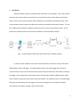
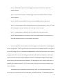
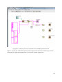
Fig 1 – Context Diagram of Real Time Data retrieval from a Weather Station
In order to create a weather station that relays the data to the internet in real time we used a
HOBO weather station and logger. The HOBO weather station was a data logger that connects to
various weather sensors and records the data at preset intervals and stores the information in memory.
The logger is then queried for the information stored. The particular model of HOBO weather station
that we used for the project comes with a wireless RF module. This module connects to the data logger
and relays the information from the logger to a computer through the use of another RF module
connected to the computer through a serial or RS 232 port.
2
In order to communicate with the data logger we used the Onset remote monitoring software to
setup an auto readout schedule. This automatically queries the data logger for the weather data every
20 seconds and stores this data in an XML file. Once the data is in XML format we used a Java program
to parse the information and store it in our mySQL database. The pseudo code for this program is the
following:
while(true){
open the Xml file;
Read last sensor entry;
Check to see if the last entry is the same timestamp as the new entry
if(new entry Date!=old entry Date){
insert data into mySQL database;
new entry Date= old entry Date;
}
close the XML file;
}//End Pseudo code
As you can see this from the pseudo code this program runs in a loop. Each pass through the loop the
program opens the XML file and read in the last sensor entry. If this entry is not the same as the last
entry read in by the program then it enters the information into the mySQL database. Then the program
closes the XML file and repeats itself.
3
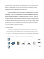
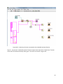
Once the information is in a database a PHP website interacts with the database to display the
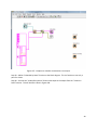
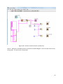
information via the internet. Figure 2 is a logical diagram of the system.
Figure 2 – Logical Diagram of Problem Solution
Since the largest delay in the transfer of the weather data is that the HOBO software only queries the
data logger to retrieve the data every 20 seconds and all of the other processes will be executed quickly
the weather data will be displayed on the internet within approximately 30 seconds. Since the
information that we will be recording, like temperature and humidity, does not change by a large
amount in a short amount of time this system can be considered near real time.
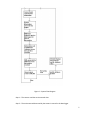
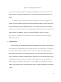
System Flow Diagram
4
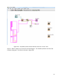
Figure 3 – System Flow Diagram
Step 1 – The sensors read the environmental data
Step 2 – The environmental data read by the sensors is stored in the data logger
5
Step 3 – HOBO software queries the data logger to send the information to it across the
wireless network.
Step 4 – The stored information in the data logger is sent to the HOBO software across the
wireless network.
Step 5 – XML file containing the information received by HOBO software is generated.
Step 6 – The Java program reads in the XML file and checks if the information is new. If it is new
the system goes on to step 7 otherwise if it is not new it returns to step 1
Step 7 – mySQL database is updated by the Java program to contain the new data
Step 8 – Website displays the information stored in the mySQL database. The newest entry in
the mySQL database will be the current weather information.
The Java program to input the data from the data logger into the database for the webpage can
be seen in Appendix B. In this program it opens a file obtained from the HOBO software containing all of
the sensor readings. This file is created by the HOBO software and sent to the computer. Once the Java
program opens this file it parses the readings into variables and transforms the date/time information
into the correct format for the mySQL database. Once this is completed the program creates mySQL
queries to enter the information into the database. The Java program runs in a loop so once the file is
updated it will update the database. This is done in order to keep the current sensor readings stored
into the database.
The database that is created for this project is only 1 table. It is comprised of 4 columns. These
four columns are: timestamp, pressure, temperature, and relative humidity. The timestamp holds the
6
information about the exact time when the sensor readings were taken. The timestamp column in the
database can only store unique entries, since only unique timestamps are stored there is no need to
handle duplicate entries in the database because there will be none.
Using the information that is stored on the database current weather information is displayed
on the webpage. In order to do this the webpage has to connected to the database and determine the
latest entry based off of the timestamps. This webpage code can be seen in Appendix B. Another way
to display the information stored in the database is through graphs of the data sets. Appendix C is code
for a webpage that displays a graph for 12 hours worth of data. When this page is first loaded it displays
graphs of the oldest 12 hours in the database but allows a client to select and offset based on hours so
all of the data stored into the database can be selected.
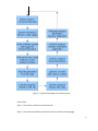
2. Problem Description
For this project we are going to implement an alternative method to view real time weather
information obtained from the HOBO weather station via the internet. Some of the setup will be
the same as the previous example but instead of using a Java program, database, and PHP webpage
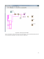
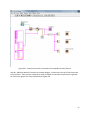
we will be using Labview. A diagram of this system can be seen in the figure below.
7
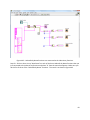
Figure 4 – Logical Diagram of Problem
As you can see in the above diagram the right half of the problem solution will be the same as the
previous solution. The part that is different is from the left half from the Labview program to the
clients.
To develop the system to deliver the weather information to the client the program will
need to start from the XML file generated by the Onset HOBOware software. This XML file contains
all of the data obtained from the HOBO data logger. So the system will need to open the XML file
and parse it into a usable form of data. Once the data from the XML file has been converted we will
need to display it on a webpage. Also, all of this needs to be done in real time. Once the
information is on a webpage clients will be able to view the weather data in real time from the
HOBO weather station.
3. Problem Solution
In order to read in the XML file and generate the webpage we will use Labview. Labview has the
ability to generate embedded applications using data sockets for use in web pages. The applications
are able to be controlled from anywhere via the internet. So we will have the Labview program
open the XML file and parse it into a usable data format. Then it will store the data into a cluster in
order to be able to be used by the Labview software. We will then use the Labview ability to create
an embedded application that will be able to be controlled by the clients over the internet. The
Labview program will display the information in an easily readable format and allow the clients to
view all of the weather data not just the latest data. Below is a system flow diagram of this problem
solution.
8
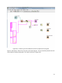
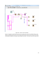
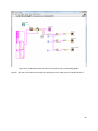
Figure 5 – System Flow Diagram of problem solution
System Flow
Step 1 – The sensors read the environmental data
Step 2 – The environmental data read by the sensors is stored in the data logger
9
Step 3 – HOBO software queries the data logger to send the information to it across the
wireless network.
Step 4 – The stored information in the data logger is sent to the HOBO software across the
wireless network.
Step 5 – XML file containing the information received by HOBO software is generated.
Step 6 – Labview reads in the XML file
Step 7 – Labview parses the data from the XML file so it can be manipulated
Step 8 – Labview converts data from XML file into clusters so it can use the data
Step 9 – Labview generates graphs for easy display of information from the XML file
Step 10 – Labview generates an embedded application to display the information
Step 11 – Webpage displays the Labview program by using the embedded application
Step 12 – System runs in a loop to update information
4. Implementation
XML parsing is very difficult in Labview. It is a lot more complex then it needs to be and National
Instruments is working on it always updating XML to make it easier each time with each new
version. Currently if you want to read in an XML file the best way to do this is to use the JKI Easy
XML VI. The Easy XML vi takes an XML string format and parses it into a cluster or array, whichever
you declare. For this project we are using the evaluation version of this vi which is free and can be
obtained from http://jkisoft.com/easyxml/. We open the XML file using Labview just like any
10
normal file and send the variable to through the Easy XMl vi. We have the VI output a cluster
containing all of the information that was in the XML file. Since we now have the XML data in a
format that is usable in Labview we can manipulate the data however we would like. We created
graphs displaying all of the data obtained from each sensor and plotted it against the time it was
taken to show how the readings have changed over time. This programs front panel and block
diagram can be seen in Appendix A and a step by step guide on how this program was developed is
in Appendix B.
Once we have our Labview program running correctly we worked on displaying this
information via the web. Labview can host web pages and uses data sockets to display the program
as an embedded application in a webpage. In order to do this we use Labview web publishing tool
which creates a webpage in the hosted folder. This webpage is a simple html webpage that contains
a table with an embedded object that is the embedded application from the vi. Then we are able to
take this code and place it into our own webpage to display the embedded application in any
website that we desire. The simple webpage html code created by the web publishing can be seen
at the bottom of Appendix A.
5. User Manual and Example of Use
5.1
Hardware Configuration
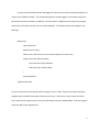
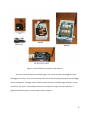
This project uses the Onset HOBO micro weather station. The Onset HOBO micro weather
station consists of a data logger, a temperature sensor, a relative humidity/pressure sensor, and two rf
radio modules. Figure 6 shows the different pieces of the HOBO micro weather station.
11
Figure 6 – Onset HOBO micro weather station devices
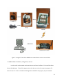
The sensors connect directly to the data logger. Four sensor are able to be plugged into the
data logger at one time. They use a connection much like an Ethernet plug and plug into the data logger
next to the batteries. The larger of the rf radio modules connects to the data logger through a custom
connection. The other rf radio module connects to a computer through a serial port (RS 232). A
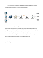
diagram of how these pieces are connected is shown in Figure 7.
12
Figure 7 – Diagram of how Onset HOBO micro station devices connects to each other
5.2 HOBO Software Installation, Configuration, and Use
In order to talk to the weather station we have to use Onset’s software. First install the Onset
Remote Site Manager. To install this program insert the cd-rom and run the setup.exe program, if it
does not auto run. There is no advanced configuration needed for this program, so just remember
13
where you install it to so you can run the program later. The next program that needs to be installed is
Onset’s HOBOware software. To install this software insert the HOBOware cd-rom and run the
setup.exe program, if it does not auto run. HOBOware has no advanced configuration needed, just
remember where it is installed to so it can be run at a later time. The last software needed for this
project besides Labview is the EasyXML Toolkit for Labview. This toolkit was developed by JKI Software
and a free evaluation copy is available to download. In order to install this toolkit you will need to get
their free VI Package Installer which can be obtained at this website (http://www.jkisoft.com/vipm/).
Click on the “Download VI Manager” and fill out the required information. Once downloaded run the
setup and install the VI Package Manager. Once installed run the VI Package Manager program. Now go
to Tools in the top menu and select “Check the Network for Available Packages”. This will update the list
of available packages for you to install. From the list find the one that says “jki_lib_easyxml” and select
it. Now go to the top menu and select Package then install. This will install the toolkit into Labview and
will grant access to the EasyXML vi’s for use. This software is all you will need for this project.
There are two choices for communication with the HOBO, HOBOware and Remote Site
Manager, but for this project we will use both HOBOware and Remote Site Manager. First we need to
setup the data logger to record information from the sensors. In order to do this we will use
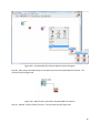
HOBOware. Start HOBOware by double clicking on the HOBOware icon. As a result, a screen shown in
Figure 8 appears.
14
Figure 8 – HOBOware starting screen
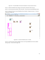
Now at the top menu from Figure 8, go to device and select “Launch”. This will Launch Logger screen
shown in Figure 9.
15
Figure 9 – Launch Logger screen from HOBOware
On this screen under “Channels to Log” make sure all of the desired sensors that you want to log are
checked. It is recommended to select all of the sensors. Now select how often you would like the data
logger to log sensor information by changing the “Logging Interval”. For this project we select 1 minute.
Once the Logging interval is selected we need to decide on a Launch option. Select the radial next to
“Now” to start logging information immediately. Once you have done this, click on the “Launch” button
at the bottom of the screen. Now the program will take some time to configure the data logger. Once
16
the data logger is launched, which is indicated by the appearance of a status bar, you may close
HOBOware, by selecting Exit menu choice from the screen as shown in Figure 6.
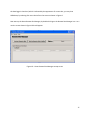
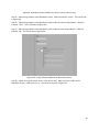
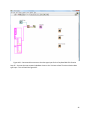
Now start up the Onset Remote Site Manager, by double clicking on the Remote Site Manager icon. As a
result a screen shown in Figure 10 should appear.
Figure 10 – Onset Remote Site Manager startup screen
17
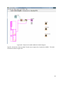
Once the Remote Site Manager is running we need to create a remote site. In order to do this click on
the “Set up remote site profiles” button and a screen will appear, as shown in Figure 11.
Figure 11 – Remote Profile page from Remote Site Manager program
18
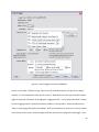
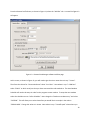
From the Remote Profile Screen, as shown in Figure 11, select the “Add Site” tab. A screen like Figure 12
will appear.
Figure 12 – Remote Site Manager software Add Site page
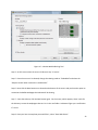
At this screen, as shown in Figure 12, you will need to give the site a name where it says “* Name”.
Then from the choices for “Connection Route” select “Local Port”. Now where it says “* COM Port”
select “COM 1” or which serial port that you have connected the radio module to. The Auto-Readout
Schedule will need to be setup in order for the program to auto readout. To setup the auto readout
select the checkbox next to “Utilize Schedule”. Next change the “Read out new data every” and select
“CUSTOM”. This will allow you to select how often you would like it to sample in the column
“DDD:HH:MM”. Change this value to 1 minute. Now where it says “* Datafile path” select where you
19
would like to save the XML file containing the sensor data that this software is generating. Once you
have these parameters filled out click “OK” button. From this screen click “Connect” and a screen like
Figure 13 will appear. This page is attempting to connect to the data logger and it should connect if the
parameters are correct.
Figure 13 – Remote Connection page from Remote Site Manager
If the parameters are not correct it will tell you that it is not connected. If this is the case, edit your
parameters to the correct ones. Once you have the remote site connected to, close the screen, Figure
13. Now you will be back at a screen like Figure 8. Here you should see the site you just created in the
“Auto-Readout Schedule”. Click on the “activate” box and select the correct remote site to activate.
5.3 Labview Software Operation
Once the Remote Site Manager is running an auto-readout you need to run the Labview program. All
respective user actions are described in the following steps.
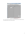
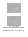
Step 1 - Open up the Labview program and you will see a screen like in Figure 14.
20
Figure 14 – Labview User program front panel screen
Step 2 - Now you need to select where you told the Remote Site Manager software to output the data
to. To do this change the “XML File Path” to the correct location where the XML file is.
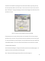
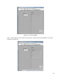
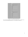
Step 3 - Now to get the application to be displayed on a webpage select Tools -> Web Publishing Tool
from the Labview screen. This will bring up a screen shown in Figure 15.
21
Figure 15 – Labview Web Publishing Tool
Step 4 - At this screen select the correct VI where it says “VI name”.
Step 5 - Once the correct VI is selected, change the viewing mode to “Embedded” and select the
“Request control when connection is established.”
Step 6 - Now click the Next button once located at the bottom of the screen and you have the option to
customize the default webpage that Labview will be hosting.
Step 7 – Once that is done, click the Next button again. On the screen, which appears, when it asks for
the directory to save the webpage make sure it is in the root folder. Labview will give you a notification
if it is not.
Step 8 - Once you have it setup how you would like it, select “Start Web Server.”
22
Step 9 – Press the “Save to Disk” button to save the webpage.
Step 10 – This will bring up a notification and give two options. Select the “Connect” button to connect
to the webpage to ensure that it is working properly. If this screen does not appear open up Internet
explorer and go to the URL where the webpage is hosted to make sure everything is working correctly.
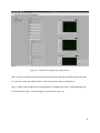
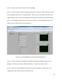
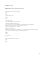
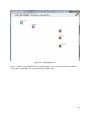
Step 11 – The webpage should look like the one shown in Figure 16. On this webpage locate the file
folder next to the “XML File Path” text box and click it.
Figure 16 – Simple Webpage with Labview Embedded Application
Step 12 – A screen will appear asking where you saved the XML file generated by the Remote Site
Manager. Find where you saved this XML file and select it. Then click the “Open” button.
Step 13 – At the top of the embedded application click the menu “Operate” and select “Run”. The
webpage will read in the information in the XML file now.
23
Step 14 – If a popup appears click the button that says “Continue Evaluating”.
Step 15 – Once the data has been parsed by the Labview program you can look at the overall data for
each of the sensors on the three graphs on the right. Each graph is for a specific sensor and is labeled.
Step 16 – The box “hoboData” contains all of the information parsed form the XML file. Here you can
see the basic information about the data logger and the start time and ending time of the data that was
gathered from the sensors. Also, it tells you the interval between measurements of the data.
Step 17 – Under “hoboData” there is another box that is labeled “sensor”. The numeric control next to
this box allows you to switch between the three sensors by selecting 0, 1, or 2.
Step 18 – At the bottom of each of the sensor boxes there is a section labeled “d”. This is the individual
data measurements. To scroll through them change the numeric control to the left of the text box.
6. Conclusion
This project has been a success creating a system that will display the information online in real
time using Labview. The system might not display the information in true real time but it display the
information once every minute. This was decided that once a minute was a short enough interval
that it can be considered real time since weather information does not change by large amounts in
short periods of time. The project would still need some more work mostly on displaying the
information on the front panel in order to be a true finished project. Other things could be changed
on the front panel to make viewing the specific sensor information easier. Also timestamps could be
added to each sensor reading display so you can tell exactly what time the information was taking
24
instead of having to figure it out by the starting time and how many intervals you are past the
starting time.
25
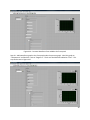
Appendix A: Labview Program
Screen Shot of Block Diagram of Labview program
Screen Shot of Front Panel of Labview Program
26
Appendix A: Continued
Webpage Code: Created by Labview Web publishing tool
<!DOCTYPE HTML PUBLIC "-//W3C//DTD HTML 3.2 Draft//EN">
<HTML>
<HEAD>
<TITLE>Title of Web Page</TITLE>
</HEAD>
<BODY >
<H1>Title of Web Page</H1>
Text that is going to be displayed before the VI panel image.<P>
<TABLE BORDER = 1 BORDERCOLOR = #000000><TR><TD>
<OBJECT ID="LabVIEWControl" CLASSID="CLSID:A40B0AD4-B50E-4E58-8A1D-8544233807AF" WIDTH=1434 HEIGHT=843
CODEBASE="ftp://ftp.ni.com/support/labview/runtime/windows/8.5/LVRunTimeEng.exe">
<PARAM name="LVFPPVINAME" value="hobo___EasyXML2.vi">
<PARAM name="REQCTRL" value=true>
<EMBED SRC=".LV_FrontPanelProtocol.rpvi85" LVFPPVINAME="hobo___EasyXML2.vi" REQCTRL=true TYPE="application/x-labviewrpvi85"
WIDTH=1434 HEIGHT=843 PLUGINSPAGE="http://digital.ni.com/express.nsf/bycode/exck2m">
</EMBED>
</OBJECT>
</TD></TR></TABLE>
<P>
Text that is going to be displayed after the VI panel image.
</BODY>
</HTML>
27
Appendix B: Creation of Labview Program
Step 1: Select “Blank VI” from under New on the Labview startup screen
Step 2: Add a file path control to the front panel and label it “XML File Path”. The file path control can
be found under Express->Text Control. The front panel should now look like it does in Figure A1.
Figure A1 – File path control added to Labview blank program
Step 3: Add a cluster and label it “hoboData”. This can be seen in Figure A2.
28
Figure A2 – Cluster added to program
Step 4 – Create another cluster inside of the cluster that you have just created and label it index. The
result should look like the screen as shown in Figure A3.
29
Figure A3 – info cluster added
Step 5 – Create another cluster inside of the info cluster. Label this new cluster #attributes. The result
can be seen in Figure A4.
30
Figure A4 - #attributes cluster added
Step 6 – Add a string indicator inside of the info cluster. Label this string indicator “sn”. The result can
be seen in Figure A5.
Step 7 – Add a string indicator inside of the info cluster but below the sn string indicator. Label this
string indicator “desc”. The result can be seen in Figure A5.
Step 8 – Add a string indicator inside of the info cluster but below the desc string indicator. Label this
string indicator “zone”. The result can be seen in Figure A5.
Step 9 – Add a string indicator inside of the info cluster but below the zone string indicator. Label this
string indicator “interval”. The result can be seen in Figure A5.
Figure A5 – string indicators added to the #attributes cluster
Step 10 – Under the info cluster but inside the hoboData cluster add a string indicator and label it
“start”. This can be seen in Figure A6.
31
Figure A6 – start string indicator added inside the hoboData cluster
Step 11 – Under the start string indicator add another string indicator and label this one end. This can
be seen in Figure A7.
32
Figure A6 – end string indicator added
Step 12 – Inside of the hoboData and under the end string indicator add an array. The result should be
like the screen shown in Figure A7.
33
Figure A7 – array added to the hoboData cluster
Step 13 – Create a cluster inside of the sensor array. Label this cluster sensor. The result should look like
it does in Figure A8.
34
Figure A8 – sensor cluster added to sensor array
Step 14 – Create a cluster inside of the sensor cluster. Label this cluster #attributes. The result should
look like it does in Figure A9.
35
Figure A9 - #attributes cluster added to the sensor cluster in sensor array
Step 15 – Add a string indicator to the #attributes cluster. Label the indicator “name”. This can be seen
in Figure A10.
Step 16 – Add a string indicator to the #attributes cluster under the name string indicator. Label the
indicator “units”. This can be seen in Figure A10.
Step 17 – Add a string indicator to the #attributes cluster under the units string indicator. Label the
indicator “SN”. This can be seen in Figure A10.
Figure A10 – string indicators added to the #attributes cluster
Step 18 – Add an array to the sensor cluster in the sensor array. Make sure not to add it to the
#attributes cluster. Label this array “d”. The result can be seen in Figure A11.
36
Figure A11 – Array added to the sensor cluster
Step 19 – Add a numeric indicator to the d array. The result should look like it does in Figure A12.
Figure A12 – numeric indicator added to d array
Step 20 – Select the whole sensor array and go to the top menu and select “Edit”. Then go down and
select “copy”.
Step 21 – Now go to “Edit” and select “paste”. This will copy the sensor array.
Step 22 – Change the label on the new sensor array to “calc”. Move this array to be under the sensor
array but inside of the hoboData cluster. It should look like the screen in Figure A13.
37
Figure A13 – calc array added to the hoboData cluster
Step 23 – Add a waveform graph to the front panel. Label this graph as “Pressure” and label the Y axis
as “Hg”. The X axis should be left labeled as “Time”. This step can be seen in Figure A14.
38
Figure A14 – Pressure Waveform Chart added to the front panel
Step 24 – Add a waveform graph to the front panel under the pressure graph. Label this graph as
“Temperature” and label the Y axis as “Degrees F”. The X axis should be left labeled as “Time”. This
step can be seen in Figure A15.
39
Figure A15 – Temperature waveform graph added to the front panel
Step 25 – Add a waveform graph to the front panel under the Temperature graph. Label this graph as
“Relative Humidity” and label the Y axis as “Percent %”. The X axis should be left labeled as “Time”. This
step can be seen in Figure A16.
Figure A16 – Relative Humidity waveform graph added to the front panel
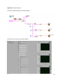
Step 26 – Now go the block diagram for this VI. To do this go to “Window” at the top menu and select
“Show block diagram”. A screen like in Figure A17 will appear.
40
Figure A17 – Block diagram of VI
Step 27 – Add the “Easy Read XML File” to the block diagram. This can be found under the Functions>JKI Toolkits->JKI EasyXML. The result should look like Figure A18.
41
Figure A18 – Easy Read XML File function added to the block diagram
Step 28 – Now connect the XML file path to the path input on the Easy Read XML File function. The
result will look like Figure A19.
Figure A19 – XML file path connected to Easy Read XML File function
Step 29 – Add the “Variant to Data” function. The result will look like Figure A20.
42
Figure A20 – Variant to Data function added
Step 30 – Connect the “Easy Read XML File” function data output to the “Variant to Data” Function data
input. Also connect the “Easy Read XML File” function error output to the “Variant to Data” Function
error input. The result will look like Figure A21.
43
Figure A21 – “Easy Read XML File” function connected to “Variant to Data” function
Step 31 – Select the hoboData cluster and go to the top menu and select “Edit” then copy.
Step 32 – Go to the top menu and select “Edit” then paste. This will create a second hoboData cluster.
Step 33 – Now right click on the second hoboData cluster and select “Change to constant”. The result
should look like Figure A22.
Figure A22 – A constant hoboData cluster is created
Step 34 – Connect the new constant hoboData cluster to the “Easy Read XML File” function Labview
data type input. This will look like Figure A23.
44
Figure A23 – Connected the constant to the data type input for the Easy Read XML File function
Step 35 – Connect the new constant hoboData cluster to the “Variant to Data” function Labview data
type input. This will look like Figure A25.
45
Figure A24 - Connected the constant to the data type input for the Variant to Data function
Step 36 – Connect the “Variant to Data” data output to the hoboData cluster. The result will look like
Figure A25.
46
Figure A25 – “Variant to Data” function output connected to hoboData cluster
Step 37 – Add a “simple error handler” function to the block diagram. The result will look like it does in
Figure A26.
47
Figure A26 – Simple error handler added to the block diagram
Step 38 – Connect the “Variant to Data” function error output to the “simple error handler. The result
will look like it does in Figure A27.
48
Figure A27 – Simple error handler connected to error output
Step 39 – Add an “Unbundle by Name” function to the block diagram. This is a function to use only a
part of a cluster.
Step 40 – Connect the “Unbundle by Name” function data input to the output from the “Variant to
Data” function. This will look like it does in Figure A28.
49
Figure A28 – “Unbundle by Name” connected to the “Variant to Data” output
Step 41 – Now we need to configure what the “Unbundle by Name” function selects. To do this right
click on the “Unbundle by Name” function and click on “Select Item”. This will bring up another menu
and click on “sensor”. The result can be seen in Figure A29.
50
Figure A29 – Unbundle by Name function edited to select the “sensor” data
Step 42 – Add an “Index Array” function to the block diagram. This should be placed to the left of the
Pressure wave graph. The result can be seen in Figure A30.
51
Figure A30 – Index Array function added
Step 43 - Add another “Index Array” function to the block diagram. This one should be placed to the left
of the Temperature wave graph. The result can be seen in Figure A31.
52
Figure A31 – Index Array function added to the left of Temperature wave graph
Step 44 - Add another “Index Array” function to the block diagram. This one should be placed to the left
of the Relative Humidity wave graph. The result can be seen in Figure A32.
53
Figure A32 – Index Array function added to the left of Relative Humidity wave graph
Step 45 – Connect the “Unbundle by Name” function output to the input of the “Index Array” function
to the left of the Pressure wave graph. The result can be seen in Figure A33.
54
Figure A33 – Index Array function connected to the Unbundle by Name function
Step 46 – Connect the “Unbundle by Name” function output to the input of the “Index Array” function
to the left of the Temperature wave graph. The result can be seen in Figure A34.
55
Figure A34 – Index Array function connected to the Unbundle by Name function
Step 47 – Connect the “Unbundle by Name” function output to the input of the “Index Array” function
to the left of the Relative Humidity wave graph. The result can be seen in Figure A35.
56
Figure A35 – Index Array function connected to the Unbundle by Name function
Step 48 – Add three Numeric Constants to the block diagram. Place these to the left of the three Index
Array functions. These numeric constants are used as indexes for the Index Array function to get data
for each sensor graph. The result should look like Figure A36.
57
Figure A36 – Numeric Constants added
Step 49 – Change the second from the top numeric constant to the value of 1 by double clicking on the
number and entering the new value. Also, change the third from the top numeric constant to the value
of 2 by double clicking on the number and entering the new value. The result can be seen in Figure A37.
58
Figure A37 – Numeric constants are given values
Step 50 – Connect the top numeric constant with the value of 0 to the Index Array to the left of the
Pressure Wave graph. This result can be seen in Figure A38.
59
Figure A38 – Numeric Constant connect to Index Array
Step 51 – Connect the second from the top numeric constant with the value of 1 to the Index Array to
the left of the Temperature Wave graph. This result can be seen in Figure A39.
60
Figure A39 – Numeric Constant connect to Index Array
Step 51 – Connect the bottom numeric constant with the value of 2 to the Index Array to the left of the
Relative Humidity Wave graph. This result can be seen in Figure A40.
61
Figure A40 – Numeric Constant connect to Index Array
Step 52 – Add three “Unbundle by Name” functions to the block diagram. One to the left of each of the
wave graphs. This can be seen in Figure A41.
62
Figure A41 – Three unbundled by name functions are added
Step 53 – Connect the three “Unbundle by Name” functions that you just added to the “Index Array”
functions output that are to the left of each function. The result can be seen in Figure A42.
63
Figure A42 – Unbundle by Name functions are connected to the Index Array functions
Step 54 – Click on where it says “#attributes” on each of the three Unbundle by Name functions that you
just connected to the Index Array functions and select “d” from the menu that appears. Make sure you
do this for all three of the “Unbundle by Name” functions. The result is as shown in Figure A43.
64
Figure A43 – Unbundle by Name function values changed to “d”
Step 55 – Now connect each of the three “Unbundle by Name” functions output to the waveform graphs
input to the right of them. The result is shown in Figure A44.
65
Figure A44 – Unbundle by Name functions connected to their corresponding graphs
Step 56 – Run the VI and make sure everything is working correctly. Now you are finished with this VI.
66
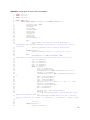
Appendix C: Java program to enter results into database
1.
2.
3.
4.
5.
6.
7.
8.
9.
10.
11.
12.
13.
14.
15.
16.
17.
18.
19.
20.
21.
22.
23.
24.
25.
26.
27.
28.
29.
import java.sql.*;
import java.io.*;
import java.util.*;
public class hobo {
public static void main(String[] args) throws SQLException {
Connection conn = null;
String dateTime;
String RH;
String temp;
String pressure;
String text;
String month;
String day;
String year;
String time;
String tempTime ="";
try {
Class.forName ("com.mysql.jdbc.Driver").newInstance ();
conn =
DriverManager.getConnection("jdbc:mysql://mysql.spoatacus.com/okeen_hobo", "okeen" ,
"2CbhJuL#");
System.out.println("Database Connection Established");
}
catch(Exception x){
System.out.println( "Unable to load the driver class!" );
}
try {
BufferedReader in = new BufferedReader (new
FileReader("C:\\Documents and Settings\\Kyle\\My Documents\\hobo\\test_1.txt"));
30.
31.
32.
33.
34.
35.
36.
37.
38.
39.
40.
41.
text = in.readLine();
text = in.readLine();
text = in.readLine();
text = in.readLine();
text = in.readLine();
while (in.ready()) {
text = in.readLine();
System.out.println(text);
StringTokenizer st = new StringTokenizer(text, "\t");
dateTime = st.nextToken();
StringTokenizer token = new StringTokenizer(dateTime, "/
");
42.
43.
44.
45.
46.
47.
48.
49.
50.
51.
52.
53.
54.
55.
56.
57.
58.
59.
60.
month = token.nextToken();
day = token.nextToken();
year = token.nextToken();
time = token.nextToken();
dateTime = year + "/" + month + "/" + day + " " + time;
pressure = st.nextToken();
System.out.println(pressure);
temp = st.nextToken();
RH = st.nextToken();
Statement stmt = conn.createStatement();
ResultSet rs;
rs = stmt.executeQuery("SELECT timestamp FROM sensor_temp
ORDER BY timestamp DESC LIMIT 1");
stmt.executeUpdate("INSERT INTO sensor_temp ( timestamp,
pressure, temperature, rh ) VALUES ( \""+ dateTime+ "\", "+ pressure+ ", "+temp+", "+RH+"
)");
}
in.close();
}
catch (Exception e){
System.out.println(e);
67
61.
62.
63.
64.
65.
66.
67.
68.
69.
70.
71.
72.
}
if (conn != null)
{
try
{
conn.close ();
System.out.println ("Database connection terminated");
}
catch (Exception e) { /* ignore close errors */ }
}
}
}
68
Appendix D: index.php
1.
2.
3.
4.
5.
6.
7.
8.
9.
10.
11.
12.
13.
14.
15.
16.
17.
18.
19.
20.
21.
22.
23.
24.
25.
26.
27.
28.
29.
30.
31.
32.
33.
<html>
<head>
<link rel="stylesheet" type="text/css" href="style.css" />
<title> Sample Weather Information </title>
</head>
<body>
<div class="outer">
<div id="banner">
<span><br>HOBO Weather Station</span>
</div>
<div id="menu">
<ul>
<li><a href="http://okeen.spoatacus.com/hobo/">Home</a></li>
<li><a href="http://okeen.spoatacus.com/hobo/graph.php">Graphs</a></li>
<li><a href="http://okeen.spoatacus.com/hobo/about.html">About</a></li>
<li><a href="http://okeen.spoatacus.com/hobo/contact.html">Contact us</a></li>
</ul>
</div>
<?php
$dbhost = 'mysql.spoatacus.com';
$dbuser = 'okeen';
$dbpass = '2CbhJuL#';
$conn = mysql_connect($dbhost, $dbuser, $dbpass) or die
connecting to mysql');
('Error
$dbname = 'okeen_hobo';
mysql_select_db($dbname);
?>
<?php
$query = "SELECT timestamp, pressure, temperature, rh FROM sensor_temp ORDER BY timestamp
DESC LIMIT 1";
34. $result = mysql_query($query);
35. $row = mysql_fetch_array($result, MYSQL_ASSOC);
36.
37.
echo "<h3> Current Weather Station Sensor Reading</h3>";
38.
echo "Time : {$row['timestamp']} <br>" .
39.
"Pressure : {$row['pressure']} <br>" .
40.
"Temperature : {$row['temperature']} <br>" .
41.
"Relative Humidity : {$row['rh']} <br>";
42. ?>
43. </div>
44. </body>
45.
46. </html>
69
Appendix E: graph.php
1. 1.<?php
2.
$time = $_GET['time'];
3.
$time = $time*60;
4.
/* Connect to the MySQL Database Server */
5.
$link = mysql_connect("mysql.spoatacus.com", "okeen", "2CbhJuL#")
6.
or die("Could not connect : " . mysql_error());
7.
8.
/* Select Database*/
9.
mysql_select_db('okeen_hobo',$link) or die("Could not select database");
10.
11.
/* Performing SQL query for Product X*/
12.
$query = "Select distinct timestamp, temperature FROM sensor_temp ORDER BY timestamp
DESC";
13.
$result1 = mysql_query($query) or die("Query failed : " . mysql_error());
14.
$query = "Select distinct timestamp, pressure FROM sensor_temp ORDER BY timestamp
DESC";
15.
$result2 = mysql_query($query) or die("Query failed : " . mysql_error());
16.
$query = "Select distinct timestamp, rh FROM sensor_temp ORDER BY timestamp DESC";
17.
$result3 = mysql_query($query) or die("Query failed : " . mysql_error());
18.
19.
/* Construct HTML page containing Line Graph Applet*/
20.
print "<html>\n";
21.
print "<head>\n"; ?>
22.
<link rel="stylesheet" type="text/css" href="style.css" />
23. <?php
24.
print "<title>Sensor Reading Graphs</title>\n";
25.
print "</head>\n";
26.
print "<body>\n";
27.
print "<div class='outer'>\n";
28.
print "<div id='banner'>\n";
29.
print "<span><br>HOBO Weather Station</span>\n";
30.
print "</div>\n";
31.
print "<div id='menu'>\n";
32.
print "<ul>\n";
33.
print "<li><a href='http://okeen.spoatacus.com/hobo/'>Home</a></li>\n";
34.
print "<li><a href='http://okeen.spoatacus.com/hobo/graph.php'>Graphs</a></li>\n";
35.
print "<li><a href='http://okeen.spoatacus.com/hobo/about.html'>About</a></li>\n";
36.
print "<li><a href='http://okeen.spoatacus.com/hobo/contact.html'>Contact
us</a></li>\n";
37.
print "</ul>\n";
38.
print "</div>\n";
39.
40.
41.
print "<br>\n";
42.
print "<form>\n";
43.
print "Displace the graph by hours (displays 12 hours of data): <input type='text'
name='time' />\n";
44.
print "<input type='submit' />";
45.
print "</form>\n";
46.
print "<br>\n";
47.
print "<div id='graphContent'>\n";
48.
print "<applet code='LineGraphApplet.class' width='600' height='420'>\n";
49.
print "
<!-- Start Up Parameters -->\n";
50.
print " <PARAM name='LOADINGMESSAGE' value='Line Graph Loading - Please Wait.'>
<!-- Message to be displayed on Startup -->\n";
51.
print " <PARAM name='STEXTCOLOR' value='0,0,100'>
<!-- Message Text Color-->\n";
52.
print " <PARAM name='STARTUPCOLOR' value='255,255,255'>
<!-- Applet Background color -->\n";
70
53.
54.
55.
56.
57.
58.
59.
60.
61.
62.
63.
print
print
print
print
print
" \n";
" <!-- Property file -->\n";
" <PARAM name='chartproperties' value='lineproperties.php?time=".$time."'>\n";
" \n";
" <!-- Chart Data --> \n";
$data_num = 1;
$count = 1;
while ($line = mysql_fetch_array($result1, MYSQL_ASSOC)) {
if(($data_num ==1 && ($data_num>=$time)) || ($data_num%60 == 0 &&
($data_num>=$time))){
64.
print "<param name='data".$count."series1'
value='".$line["temperature"]."'>\n";
65.
$count = $count + 1;
66.
}
67.
68.
$data_num = $data_num +1;
69.
}
70.
71.
print " \n";
72.
print "</applet>\n";
73.
print " \n";
74.
print "<br>\n";
75.
print "<applet code='LineGraphApplet.class' width='600' height='420'>\n";
76.
print "
<!-- Start Up Parameters -->\n";
77.
print " <PARAM name='LOADINGMESSAGE' value='Line Graph Loading - Please Wait.'>
<!-- Message to be displayed on Startup -->\n";
78.
print " <PARAM name='STEXTCOLOR' value='0,0,100'>
<!-- Message Text Color-->\n";
79.
print " <PARAM name='STARTUPCOLOR' value='255,255,255'>
<!-- Applet Background color -->\n";
80.
print " \n";
81.
print " <!-- Property file -->\n";
82.
print " <PARAM name='chartproperties'
value='lineproperties2.php?time=".$time."'>\n";
83.
print " \n";
84.
print " <!-- Chart Data --> \n";
85.
86.
87.
$data_num = 1;
88.
$count = 1;
89.
while ($line = mysql_fetch_array($result2, MYSQL_ASSOC)) {
90.
if(($data_num ==1 && ($data_num>=$time)) || ($data_num%60 == 0 &&
($data_num>=$time))){
91.
print "<param name='data".$count."series1'
value='".$line["pressure"]."'>\n";
92.
$count = $count + 1;
93.
}
94.
95.
$data_num = $data_num +1;
96.
}
97.
98.
print " \n";
99.
print "</applet>\n";
100.
print " \n";
101.
print "<br>\n";
102.
print "<applet code='LineGraphApplet.class' width='600' height='420'>\n";
103.
print "
<!-- Start Up Parameters -->\n";
104.
print " <PARAM name='LOADINGMESSAGE' value='Line Graph Loading - Please
Wait.'>
<!-- Message to be displayed on Startup -->\n";
105.
print " <PARAM name='STEXTCOLOR' value='0,0,100'>
<!-- Message Text Color-->\n";
71
106.
print " <PARAM name='STARTUPCOLOR' value='255,255,255'>
<!-- Applet Background color -->\n";
107.
print " \n";
108.
print " <!-- Property file -->\n";
109.
print " <PARAM name='chartproperties'
value='lineproperties3.php?time=".$time."'>\n";
110.
print " \n";
111.
print " <!-- Chart Data --> \n";
112.
113.
114.
$data_num = 1;
115.
$count = 1;
116.
while ($line = mysql_fetch_array($result3, MYSQL_ASSOC)) {
117.
if(($data_num ==1 && ($data_num>=$time)) || ($data_num%60 == 0 &&
($data_num>=$time))){
118.
print "<param name='data".$count."series1'
value='".$line["rh"]."'>\n";
119.
$count = $count + 1;
120.
}
121.
122.
$data_num = $data_num +1;
123.
}
124.
125.
print " \n";
126.
print "</applet>\n";
127.
print "</div>\n";
128.
print "</div>\n";
129.
print "</body>\n";
130.
print "</html>\n";
131.
132.
/* Free resultset */
133.
mysql_free_result($result1);
134.
135.
/* Closing connection */
136.
mysql_close($link);
137.
138.
?>
72
7 References
[1]XTend Developer Kit (900 Mhz). (2007). http://www.maxstream.net/products/xtend/dev-kit.php
MaxStream, Inc.
[2] XTend OEM RF Module – Product Manua. (2007).
http://www.maxstream.net/products/xtend/product-manual_XTend_OEM_RF-Module.pdf. MaxStream,
Inc.
[3] XTend OEM RF Module (900 Mhz). (2007). http://www.maxstream.net/products/xtend/oem-rfmodule.php. MaxStream, Inc.
[4] MaxStream Product Family at ConLab. (2007). http://www.conlab.com.au/maxstream/. ConLab.
[5]High Performance Wireless Research and Education Network.(2007).
http://hpwren.ucsd.edu/news/20070130/. University of California, San Diego. (2000).
[6]High Performance Wireless Research and Education Network.(2007).
http://hpwren.ucsd.edu/news/20070130/. University of California, San Diego. (2000).
[7]EasyXML Toolkit for LabVIEW – JKI Software. (2008). http://jkisoft.com/easyxml/. JKI.
73