1
Pol-Acquisition User Manual, Birefringence Imaging
1|P a g e
Pol-Acquisition, OpenPolScope software for Micro-Manager
Last Updated: April 11, 2013; Revision 1.07
This manual was prepared based on Pol-Acquisition software version 2.0 and
Birefringence Processing enabled.
Other versions of this manual are being prepared with Dichroism Processing and with
Fluorescence Polarization Processing enabled.
Copyright, license, and warranty/disclaimer statements at end of document.
Table of Contents
Before Installation.......................................................................................................................2
Overview......................................................................................................................................4
Installation...................................................................................................................................5
Starting the Pol-Acquisition plugin........................................................................................................................ 6
The Pol-Acquisition window.................................................................................................................................... 6
A Walk-Through of Basic Operations...........................................................................................7
Calibrating the variable retarder settings........................................................................................................... 7
Acquiring birefringence images.............................................................................................................................. 9
Calibration of calculated retardance and orientation values...................................................................10
Mapping of calculated retardance and orientation values into 8-bit and 16-bit images..............10
Overview of Functionality and Interface Tabs...........................................................................11
Data tab.......................................................................................................................................................................... 11
VariLC tab...................................................................................................................................................................... 12
Controls....................................................................................................................................................................................... 12
Calibration Options................................................................................................................................................................ 13
Save & Load............................................................................................................................................................................... 14
Options........................................................................................................................................................................................ 14
Parameters tab............................................................................................................................................................ 15
Birefringence tab........................................................................................................................................................ 16
Processing tab............................................................................................................................................................. 17
Options tab.................................................................................................................................................................... 18
Logger tab..................................................................................................................................................................... 19
Acquisition Buttons................................................................................................................................................... 20
Help............................................................................................................................................23
Report Tool................................................................................................................................................................... 23
ChangeLog..................................................................................................................................................................... 24
About............................................................................................................................................................................... 25
Appendix: A................................................................................................................................26
Multi-Mode Acquisition........................................................................................................................................... 26
Appendix: B................................................................................................................................31
Calibrating the OpenPolScope for measurement of slow axis of birefringence using cheek cells
........................................................................................................................................................................................... 31
Copyright, license, warranty/disclaimer....................................................................................36
Pol-Acquisition User Manual, Birefringence Imaging
2|P a g e
Before Installation
OpenPolScope plugins come in two flavors, which are installed in different plugin folders inside
the Micro-Manager folder:
1. Pol-Acquisition plugin; after its installation into the MMplugins folder, this plugin
appears in the Micro-Manager Plugins menu. It is used to acquire PolScope images,
applying PolScope algorithms and controlling the OpenPolScope hardware attached
to the microscope.
2. Pol-Analyzer plugin; after its installation into the plugins folder, this plugin appears
in the ImageJ Plugins menu, providing functions to view and analyze PolScope data
that have been previously acquired.
The OpenPolScope software installer installs both plugins.
Software requirements:
1. Micro-Manager (tested with release 1.4.13, subsequent changes in Micro-Manager
code might result in unexpected behavior)
2. OpenPolScope software
Installer for Windows XP, 7, and Vista: LCPolScopeSetup.exe
Installer for Mac: LCPolScopeSetup.pkg
OpenPolScope software components:
Micro-Manager Plugins menu:
Pol-Acquisition, FrameAverager, TopFrame
Image J Plugins menu
PolScope: Pol-Analyzer; Orientation-Lines
PolScope Legacy: RatioAzimPolStackToRGB_V2; ROI_Averages_With_Lines_V1;
StackAverage_
Java Console
Minimum and recommended system requirements
•
Hardware:
1. OpenPolScope hardware, consisting of liquid-crystal (LC) universal compensator
and VariLC or equivalent electronic controller.
2. Camera, supported by Micro-Manager
3. Computer recommended 1.5GHz CPU dual core, 64-bit
4. 2 GB RAM (recommended 4 GB RAM)
5. 10 MB Hard Disk Space (additional space required for UserData)
Pol-Acquisition User Manual, Birefringence Imaging
•
3|P a g e
Software:
1. Windows XP, Windows 7, Mac (32/64 bit)
(OpenPolScope software is currently not tested on Mac)
2. Java 1.6 update 31
Note: It is recommended to increase the ImageJ memory (Edit>Options>Memory…) to a
minimum of 1024MB or more for smooth camera operations.
Guide to abbreviations
VariLC
Digital controller for liquid crystal devices. The controller, which might have
a name different from VariLC, is connected to the computer through a serial
or USB cable.
File naming
convention
SM_2012_0904_0213_5
Prefix_Year_MonthDate_HourMin_Suffix
Prefix:
SM – Sample
BG – Background
SMS - Sample Series
(Multi-Dimensional)
OpenPolScope data directory structure
Pol-Acquisition organizes the image data according to the following directory tree:
<LCPolScopeData> --------- (user chosen top directory)
|
<UserName1> --------- (contains directories of a single user/project)
|
<SessionDate1> --- (contains image and metadata files of a day’s session)
|
<SessionDate2>
<UserName2> --------- (contains directories of another user/project)
|
<SessionDate1> --- (contains image and metadata files of a day’s session)
|
<SessionDate2>
Pol-Acquisition User Manual, Birefringence Imaging
4|P a g e
Overview
The following schematic summarizes the hardware configuration typically required for
birefringence imaging with the OpenPolScope:
VariLC
The optical design (left) builds on the traditional polarized light microscope with the
conventional compensator replaced by two variable retarders LC-A and LC-B. The
polarization analyzer passes circularly polarized light and is typically built from a linear
polarizer and a quarter wave plate. Images of the specimen (top row, aster isolated from
surf clam egg) are captured at five predetermined retarder settings, which cause the
specimen to be illuminated with circularly polarized light (1st, left most image) and with
elliptically polarized light of different axis orientations (2nd to 5th image). The retarder
settings are computer controlled through the retarder controller, also called VariLC. Based
on the raw PolScope images, the computer calculates the retardance image and the slow
axis orientation or azimuth image using specific algorithms.
Pol-Acquisition User Manual, Birefringence Imaging
5|P a g e
Installation
For setting up the OpenPolScope hardware, the user needs to be familiar with MicroManager and its Hardware Configuration Wizard (in Tools menu). The wizard is used to
add the camera and VariLC hardware to the Micro-Manager configuration file (xxx.cfg).
These additions are necessary before the Pol-Acquisition plugin can be used. Once the
VariLC has been added, its properties have values similar to the ones seen in the image
below . The Port Properties required for communicating with the VariLC are the default
values for COM-port communication. For the Abrio, the baud rate needs to be set to
115200, instead of 9600, the total number of LCs to 3, and active LCs to 2. One can use the
Property Browser in the tools menu to test the communication with the VariLC.
Note: The VariLC is synchronized with the camera or other hardware through a delay time
setting, since the VariLC controller does not provide a state change callback. The delay time
to be used depends on the physical properties of the liquid-crystal devices. A typical delay
time is 100 ms, but can be shorter. For Abrio use 100 ms.
Before using the system, we recommend that you go through the process described
in the section “A Walk-Through of Basic Operations” to configure and calibrate the
system correctly.
Pol-Acquisition User Manual, Birefringence Imaging
Starting the Pol-Acquisition plugin
6|P a g e
The Pol-Acquisition plugin can be
accessed from the Micro-Manager
Plugins menu.
If the Pol-Acquisition plugin is
accessed without the VariLC ever
being connected to the computer
and configured as a hardware
component in Micro-Manager, an
information prompt will come up
“VariLC not detected” and VariLC
functions are disabled.
The Pol-Acquisition window
After correctly configuring the hardware,
the Pol-Acquisition plugin can be
accessed. A window opens that contains
action buttons, a progress bar, and
several tabs that let the user set
measurement parameters, settings,
options, data locations, etc.
Pol-Acquisition User Manual, Birefringence Imaging
7|P a g e
A Walk-Through of Basic Operations
While performing this sequence, you may wish to refer to the section “Overview of
Functionality and Settings Tabs”
Start the Micro-Manager software:
After the camera and VariLC controller have been turned on, you may launch the
Micro-Manager software by double-clicking the MM icon on the Windows desktop.
In the startup query window, choose the MM config file that was prepared
beforehand (see Installation) and includes the camera and VariLC controller.
Setup your sample:
Prepare your microscope for Koehler illumination. Place your sample in the field-ofview, select appropriate objective, and direct the majority of the light to the camera.
Focus on your sample using the live camera window. For calibration, move the
sample sideways out of the live camera window to image a clear, non-birefringent
sample area, also called background
Set acquisition and processing algorithms
Select the Processing tab in the Pol-Acquisition window and set Birefringence as the
acquisition and processing algorithm. For starters, deselect pre- and postprocessing algorithm(s).
A Note on Setting the Swing and Retardance Ceiling
The swing setting should be adjusted based on the sample/specimen you wish to analyze.
Thin biological samples typically require a swing of 0.03 and a retardance ceiling of 5 nm or higher.
Thicker samples or samples containing crystals should have a higher swing setting (usually 0.1).
Calibrating the variable retarder settings
At the beginning of a session, and sometimes during a session, the five liquid crystal
settings need be calibrated. Setting 0 generates circularly polarized light and is called
extinction setting for which LC-A is nominally 0.25 (quarter wave) and LC-B is 0.5 (half
wave). Settings 1 through 4 generate elliptically polarized light and LC-A and -B deviate
from the extinction values by adding or subtracting a swing value. The automatic
calibration routine optimizes the extinction and the elliptical settings, based on the swing
value chosen by the user.
The system should be calibrated while observing the slide near the area where your
sample/specimen of interest is located, as background birefringence can vary across the
slide.
Before starting calibration, make a ROI selection in the camera window that identifies a
specimen area devoid of specimen birefringence.
Identify calibration parameters:
1. Select the VariLC tab in the Pol-Acquisition Window.
2. Identify appropriate swing value. If you are unsure of this value, you may
begin by entering a median value of 0.1. Once the actual range of retardance
Pol-Acquisition User Manual, Birefringence Imaging
8|P a g e
values in your sample are known, you may adjust this number for improved
performance.
3. Check your lamp power and camera exposure time by selecting the “Check
Intensities” tab. If the intensity readings are above 210, lower the lamp
power and/or reduce exposure time.
4. Set Black Level. Block light from reaching the CCD and acquire an image.
Determine the average pixel value and enter it in the Black Level.
Recommended is a value between 3 and 7 for 8-bit images. If the value is
unacceptable, change the camera offset setting.
5. Press Calibrate. Calibration will take roughly a minute to complete.
6. Optimize exposure based upon calibrated LC settings.
With optimized exposure, the numbers from your results should be within the following
ranges (assuming 8-bit images with pixel values between 0 and 255):
LC Setting Intensity
0
1
2
3
4
10 to 80
80 to 210
80 to 210, equal to setting 2, +/- 3 cts
80 to 210, equal to setting 2, +/- 3 cts
80 to 210, equal to setting 2, +/- 5 cts
If the numbers from your results fall significantly out of the ranges shown above, you will
have to perform the calibration sequence again. Check the microscope to make sure that all
OpenPolScope components are present and that there is nothing in the optical path that may
interfere with proper operation. Be sure to remove common accessories such as filter cubes
or linear polarizers that may have been left in place by a previous user.
During calibration, if three successive measurements are too bright, the calibration will
stop and display a warning.
You may adjust the lamp and repeat the calibration sequence until all the values are in the
desired ranges. Nevertheless, even if the Average Gray values of Setting 2 through 5 are as
low as 40 or as high as 230, the OpenPolScope will still function, though not optimally.
The ratio of Setting 2 to Setting 1 is an indicator of the retardance measurement signal-tonoise ratio. Bigger ratios are better. For large retardance values, which usually involve a
retardance swing of 0.2, the ratio is 10 to 1 or better. For small retardance values, which
usually involve a retardance swing of 0.03, the ratio is typically 2 to 1 or better.
For microscope applications, the diameter of the aperture diaphragm in the condenser has
a significant impact on this ratio, and thus the retardance signal-to-noise ratio. If the
aperture is decreased, this ratio will go up. However, signal will go down and the exposure
time will increase. Of course, the adjustment of the condenser aperture will also impact
spatial resolution and depth-of-focus.
The Extinction number is another indicator of the quality of the polarization optical train.
An Extinction of at least 100 should be achieved, more routine is 200 and better. The
optical setup will be more sensitive the higher the Extinction.
Do note that if you change the swing value, you will need to recalibrate.
It is advisable to re-calibrate whenever you change the sample/specimen slide.
Pol-Acquisition User Manual, Birefringence Imaging
9|P a g e
Acquiring birefringence images
Set acquisition parameters:
Select the Parameters tab in the Pol-Acquisition window. Choose whether or not a
mirror is present in the optical path, the Black Level and the use of frame averaging
are set correctly. Please note that recalculation after image acquisition is possible
should the settings initially be incorrect (refer to Pol-Analyzer manual).
Set pre- and post-processing algorithms
Select the Processing tab in the Pol-Acquisition window and select the desired preand post-processing algorithms.
Set birefringence parameters
Select the Birefringence tab in the Pol-Acquisition window and designate an
appropriate retardance ceiling for computed retardance images. For biological
samples, this is often in the 5 – 10 nanometer range.
Acquire a background image
If the retardance values in the sample are less than 20 nm, as is often found in
biological images, we recommend that you take a background image. Background
images are taken without a sample in the field-of-view, but with the microscope
slide in place. These images are used to compensate for the birefringence of the
microscope optics themselves.
Position your sample so that the live camera window is free of sample and debris.
Defocusing slightly can help to reduce the visibility of particles in the area of the
slide where the background is acquired.
Proceed to take a background stack by clicking the BG acquisition button from the
top of the Pol-Acquisition window. The new background data will be saved to disk if
“Save to Disk Acquired Images” is checked in the Data tab.
The name of the newly acquired background stack will appear in the Background
field of the Parameters tab and will be used for background correction of the
samples subsequently acquired.
It is advisable to acquire an additional background image at the end of a time series,
as the variable retarders may drift and corrections can be applied later to
compensate for this.
Acquire a sample image
Position and focus on your sample in the Live Camera window. Proceed to acquire
an image stack by clicking the SM (sample) acquisition button from the PolAcquisition window. The newly acquired image will appear and automatically be
saved to disk if “Save Acquired Images” is checked in the Data tab.
The resulting sample image should appear in a new viewer window with
background correction applied. If no background stack is specified, the sample
retardance and orientation values are computed without background correction.
Once you have successfully acquired a sample image, you are ready to perform
Pol-Acquisition User Manual, Birefringence Imaging
10 | P a g e
Multidimensional acquisitions (e.g. z-slices, time series, etc.)
Calibration of calculated retardance and orientation values
The calculated retardance and orientation values are best calibrated against a sample for
which the retardance and slow axis orientation values are known. This is particularly
important for the slow axis orientation, which depends on physical parameters of the
optical setup, including the orientation of the liquid crystal compensator and of the camera.
The retardance values are already calibrated by virtue of the calibration of the liquid
crystal devices. The manufacturer of the LCs of the Oldenbourg Lab included a calibration
table in the VariLC controller, which allows the setting of an LC device to an absolute
retardance, usually expressed as a fraction of the wavelength. Therefore, the swing value is
given in absolute retardance, and the specimen retardance in each image pixel is calculated
in absolute retardance. (Note that the retardance of the LC-settings and the swing are given
in fraction of wavelength, while the retardance of the sample is given in nm)
The orientation of the slow axis needs to be calibrated using a specimen with known slow
axis orientation. The calibration involves the correct setting of the orientation reference
angle (see “Birefringence tab”) and of the mirror setting (see “Parameters tab”). A number
of test specimens can be used for this purpose. Biological specimens such as living (or
fixed) cells with stress fibers or dividing cells with a living spindle or well preserved
spindle microtubules are well suited, because the morphologically distinct fibers are
birefringent with a slow axis orientation parallel to the fiber axis. Also collagen fibers have
a slow axis that is oriented parallel to the fiber axis.
A simple and accurate calibration sample can be made with a thin glass fiber (e.g. soda lime
glass, diameter ~100 µm) that is taped to a microscope slide. When taping the fiber down
on both ends, induce a slight bend in the fiber. The bend causes stress birefringence whose
slow axis is oriented in a predictable fashion with respect to the fiber axis. The birefringent
layer on the outside of the bend, where the soda lime glass is stretched, has its slow axis
parallel to the fiber axis, while the birefringence in the inside layer, where the glass is
compressed, has its slow axis perpendicular to the fiber axis. For best imaging results, the
fiber can be imbibed in immersion oil to remove the cylindrical lens effect of a fiber that is
surrounded by air. (refer Appendix B for alternate method using cheek cells)
Mapping of calculated retardance and orientation values into 8-bit and 16-bit images
The calculated images in channel 1 and 2 represent the measured retardance (channel 1)
and orientation of the slow axis (channel 2) values in every pixel of the sample or
background image. As all images associated with a PolScope stack are either 8-bit or 16-bit
images, including channel 1 and 2, the calculated retardance and orientation values are
mapped into either 8-bit or 16-bit integers.
The computed retardance values are linearly mapped from 0 to the retardance ceiling
value into integer values from 0 to 255 (8-bit) or 0 to 65,535 (16-bit). Retardance values
that are computed to be higher than the ceiling value are converted to 255 or 65,535,
respectively.
A pixel value in channel 1 can be converted into a retardance value by the following
formula:
Pol-Acquisition User Manual, Birefringence Imaging
8-bit image:
retardance=
pixel_value
⋅retardance_ceiling
254
12-bit image:
retardance=
pixel_value
⋅retardance_ceiling
16,382
16-bit image:
retardance=
pixel_value
⋅retardance_ceiling
65,534
11 | P a g e
The highest possible pixel value (255 for 8-bit, 16,383 for 12-bit, and 65,535 for 16-bit
images) is reserved for indicating any value higher than the retardance_ceiling.
The computed orientation values range between 0 and 180° and are stored as integer
values from 0 to 180 (8-bit), 0 to 1800 (12-bit), or 0 to 18000 (12- and 16-bit). Hence, an
orientation angle stored in channel 2 of a 16-bit image is equal to the pixel value divided by
100.
Overview of Functionality and Interface Tabs
Data tab
The Data tab lets one choose a root
folder Data Location where
OpenPolScope data will be saved.
After selecting a root folder, User and
Session folders can be recalled in
drop-down menus or created as
needed.
Set Default to 'Save'...: Checking this
option will set the default behavior to
save acquired images into the
specified Session folder.
Session Description: This text is set
by the user when a session is created
and can be modified later to provide a
quick view description. This would
typically describe the types of
datasets or other user notes that
describes the session.
Pol-Acquisition User Manual, Birefringence Imaging
12 | P a g e
VariLC tab
This section applies when using VariLC or Abrio as a liquid crystal device controller.
Controls
The VariLC tab has controls for
the LC universal compensator
with 2 liquid crystals, LC-A and
LC-B.
Swing: Sets the nominal
retardance bias (as a fraction of
the wavelength) for the elliptical
settings of the liquid crystals.
Default is 0.03.
Wavelength: Sets the wavelength
that will be used when setting the
Retardance values. Usually equal
to center wavelength of light used
to illuminate specimen. Default is
546 nm.
Reset LC: Resets the Error light on
the VariLC controller.
Occasionally, this light might
come on during the calibration
process, without consequence.
Exercise LC: Cycles the LCs
between high/low values to assure consistent settings. Click if LCs have been powered off
for a long time and intensities measured for separate settings are not reproducible. (Click
Check several times and watch intensity values.)
LC-A and LC-B (columns): retardance values of LCs as fraction of wavelength; can be
changed by either typing value or clicking spinner wheel.
Intensity (column): intensity recorded in camera ROI; is updated each time LC retardance
is changed.
Current (row): current retardance values of LCs
The remaining buttons and fields in the lower half of the VariLC tab affect the five settings
used for OpenPolScope imaging:
Defaults: Populates the Settings with the nominal LC retardance values. The Settings are
not calibrated
Setting: Setting 0 is also referred to as the Extinction Setting. The other four Settings are the
swing applied settings that are calibrated during the calibration procedure. Clicking a
Setting button, sets the LCs to the corresponding retardance values.
Check: Measures intensities for Settings 0 through 4 and calculates the extinction
coefficient.
Pol-Acquisition User Manual, Birefringence Imaging
13 | P a g e
Calibrate: Calibrates the five LC settings using intensity readings from the camera ROI.
Calibrating the 'Extinction' Setting 0 searches for an intensity minimum by varying the
retardance values of LC-A and LC-B. The search starts from the values shown in the Current
Setting. For best results, start from a setting that is close to the minimum.
Once the Extinction values are found, the swing is applied to the next settings and
calibrated such that their intensities are equal.
Before starting calibration, make a ROI selection in the camera window that identifies a
specimen area devoid of specimen birefringence. Typically, calibration is done with the
camera showing a background region in the specimen and is immediately followed by
recording a Background stack.
Extinction field shows the extrapolated extinction coefficient. The extinction coefficient
characterizes the quality of the polarization optical train. The extinction is defined as the
ratio of the recorded intensity when the universal compensator is set to maximum
transmission divided by the intensity when the compensator is set for minimum
transmission (extinction).
is measured directly (Setting 0), while the maximum
I ext
transmission is extrapolated from Setting 1, using the measured intensity
I1
extrapolating to a virtual setting that would cause maximum transmission:
Extinction =
and
I1 + I 2 + I 3 + I 4 − 4I ext
4 ⋅ (I ext − BlackLevel)⋅ sin 2 (Swing ⋅ π )
Note: The Calibration routine can be tweaked by using the Brent Optimizer Accuracy and
Low/High range limits of the VariLC from the Options panel.
Note: It is recommended to change the VariLC settings through this tab rather than MicroManager's Device/Property Browser.
Calibration Options
Plot Intensities: Plot the Intensity profile
during Calibration.
Plot Retardance Value: Plot the Retardance
Value profile during Calibration.
Use Sequence Acquisition for Calibration: A
faster mode for Calibration and is required
enabled for certain cameras (eg. Andor). If
Calibration using this mode causes error
during Calibration you may disable it. Default is enabled.
Extinction Search: When performing a Calibration this defines the search range from
the current value. The final search range is
the multiple of swing defined. Default is 4
for Coarse and 2 for Fine.
Pol-Acquisition User Manual, Birefringence Imaging
14 | P a g e
The Brent Optimizer defines the tolerance or accuracy of the search. Default is 0.01 for Coarse and
0.00001 for Fine.
Thus with a swing of 0.03 and a factor of 4. The LC will scan a range of +/- 0.12 from the current LC
value with its respective tolerance.
Save & Load
Save VariLC Settings: A user can save
the current LC settings to a text file
with comments or Load a saved settings file (.polset). This is optional, as
the LC settings are also routinely saved
in the IJ_Prefs.txt file
Options
Device:
VariLC Range: These upper and lower
limits need to be determined for the liquid crystal devices installed and need
to be set once during installation.
Use VariLC Mapped Values: If checked,
a device specific calibration table for liquid crystal settings is used. Default is
enabled (checked). If unchecked, numbers in LC settings are sent directly to VariLC controller.
Export/Import Mapped Values Sheet: The currently used Mapped values can be exported as an excel file. A default template is exported in the case of Non-Profiled devices. This is particularly useful
for Non-Profiled LC Devices where the default values can be edited on the excel file and imported
back in the software. Imported values are not retained if Micro-Manager is restarted and the excel
file needs to be imported again.
Pol-Acquisition User Manual, Birefringence Imaging
Parameters tab
15 | P a g e
The Parameters tab includes
parameters that are used during
acquisition and are saved in the
image metadata.
Background: The selected
background that is used for
background correction when
computing the specimen
retardance and slow axis
orientation.
Note: Background data can be
stored in a file located on disk or in an open window. Background data should be recorded
at least once at the beginning of a session.
Image-Path Mirror: Used for an Inverted microscope or if there is a mirror in the optical
path. Default is No.
Setting the mirror parameter inappropriately leads to incorrectly computed orientation
values. Retardance values are not affected by the mirror setting.
Black Level: The Black Level (also called baseline) is the average pixel value when the
camera is not illuminated. The black level primarily depends on the camera offset setting.
Averaging is available if the 'FrameAverager' plugin has been installed in the MicroManager plugins folder (appears in the MM plugins folder). Averaging generates raw image
data by averaging N camera frames. Averaging reduces image noise at the expense of time
resolution. Averaging more than 8 frames is usually not effective. Default is Sample
disabled and Background enabled at 8.
Pol-Acquisition User Manual, Birefringence Imaging
16 | P a g e
Birefringence tab
The main 'Processing Mode' selected in the
Processing panel (here Birefringence) will be
displayed as an additional tab. Its panel will
contain options only applicable when this
Mode is selected.
Retardance Ceiling: Sets the value of the
retardance ceiling that is used for storing the
retardance values in its image channel
(usually first channel). For further
explanations, see section “Mapping of
calculated retardance and orientation values
into 8-bit or 16-bit images”
Orientation Reference: Sets the orientation
reference that is used for processing the slow
axis orientation image.
Use 4-Frame Acquisition...: Option to acquire only 4 frames instead of the default 5 frames,
dropping the acquisition of the raw image for Setting 4.
Use 4-Frame Processing...: Option to use only 4 frames for processing instead of the default
5 frames.
Pol-Acquisition User Manual, Birefringence Imaging
Processing tab
17 | P a g e
The Processing tab is divided into
3 main segments.
Pre-Processing: This applies some
modifications to the raw image
data before they are sent to the
main processor. An example is
Ratioing in which the pixel values
of the raw sample images are
multiplied by a correction factor
calculated based on the
background images. Multiple
Preprocessors can be selected.
preprocessing and post-processing.
Note: The raw image data that are
stored in the raw image channels
are never altered during any
processing steps, including
Processing Mode: This is the main processor, which controls the acquisition and processing
algorithms used. It defines the number of raw images acquired; the number of computed
images, which are also called virtual channels; the computation algorithm generating the
virtual channel images; along with other parameters. Only one Processor can be selected. A
Processor has its own options tab (Birefringence).
Post-Processing: This applies some post-processing correction to the images. It can also be
used to generate additional images. Multiple Post-processors can be selected.
Note: All the OpenPolScope processors that are currently installed will be displayed in this
tab.
Note: Acquisition cannot be performed without selection of a Processor plugin.
Note: Pre-/Post-Processor may or may not have additional options that are indicated by a
button.
Pol-Acquisition User Manual, Birefringence Imaging
Options tab
18 | P a g e
Multi Mode Acquisition:
For merging PolScope acquisition
with another mode of imaging,
such as fluorescence or bright
field, defined as acquisition Group.
(refer Appendix A for more
details)
Ask to merge with preconfigured
Group: allows merging with an
acquisition Group that has been
previously defined by a user.
Always ask for PolScope related Hardware Settings
on Merge: If the merge option has been used
previously the fields can be populated using the
stored values.
Display:
Show Computed Image During Acquisition: During series acquisition, this option will keep
the display on the retardance image and not display raw images. This can be changed
during series acquisitions
Processing:
Enable On-the-fly Processing during Acquisition: This option is available to disable
processing for the computed images while acquiring. In the case where acquisition speed is
extremely fast or the Image resolution is higher than usual and enough computation power
is not available, to avoid any lag that could affect acquisition this selection can be used. This
acquired dataset will then need to be Processed using the Pol-Analyzer interface. Default is
enabled.
Parallelize Processing: This option will utilize all available CPU cores for processing the
acquired images. Default is disabled.
Pol-Acquisition User Manual, Birefringence Imaging
19 | P a g e
Logger tab
This tab creates a chronological event log for the Session. The log file (session_log.txt)
resides in the User's session directory. Other than providing basic User information, all
images acquired in Micro-Manager are logged in this log file. A User can also add their own
comments and notes in the text area regarding their experiments.
Note: It is particularly useful for adding key changes to the system's hardware (eg.
Objective, Filter wheel, etc.) that are not motorized and connected to Micro-Manager and
thus their information is not logged in the image metadata.
Pol-Acquisition User Manual, Birefringence Imaging
Acquisition Buttons
20 | P a g e
SM: Acquire Sample images
BG: Acquire Background
Series...: Acquire Series/Multi
Dimensional
AutoClear: Erases the Acquisition
Comment after each acquisition.
Stop: During Acquisition the Series…
button functions as a Stop button.
(These acquisition buttons are added to the TopFrame, if it has been started.)
Note: During Series acquisition, the display of the progress bar changes with each acquired
image. However, the End Time is calculated at the start of series acquisitions and remains
fixed. If the user pauses the series acquisition, the displayed End Time will not change and
is therefore incorrect.
The Series/Multi-D Acq. uses Micro-Manager's built in Multi-D Acq. engine and dialog.
Pol-Acquisition User Manual, Birefringence Imaging
21 | P a g e
Note: The Channels settings should not
be changed at this stage.
Note: The Saving format that is used by
the PolScope plugin is 'Single-image
files' and should NOT be changed.
Pol-Acquisition User Manual, Birefringence Imaging
22 | P a g e
PolScope image stack: The
information at the bottom of a
PolScope stack includes pixel
values in terms of the
properties defined by the
processor. The Birefringence
processor will display the
Retardance value of a pixel.
Orient. Lines: This check box
causes an overlay of
orientation lines to be drawn
inside a specified ROI.
Parameters such as the line
interval are set with the
Orientation-LinesV3 plugin
button on the Viewer. In a
series, the lines are recalculated for each time-point
and/or z-slice.
The Pol-Acquisition routine writes metadata and comments in the Micro-Manager
Metadata panel.
Pol-Acquisition User Manual, Birefringence Imaging
Help
Report Tool
The Report tool can be accessed via Help in the Menu bar to send bug reports or
suggestions.
23 | P a g e
Pol-Acquisition User Manual, Birefringence Imaging
ChangeLog
24 | P a g e
Pol-Acquisition User Manual, Birefringence Imaging
About
25 | P a g e
Pol-Acquisition User Manual, Birefringence Imaging
26 | P a g e
Appendix: A
Multi-Mode Acquisition
The following steps demonstrate how to setup Micro-Manager to acquire data using other
modalities (Brightfield, Darkfield, Fluorescence, etc.) along with PolScope data using the
OpenPolScope Pol-Acquisition software.
This guide assumes the necessary hardware has been configured using the Hardware configuration
wizard.
Step 1: Start by creating a new Group using the + button and then naming eg. "Multi-D Group" and
selecting all hardware that require to be changed between acquiring PolScope dataset and other
type of datasets.
Step 2: In this example we change the Nikon TI Filter Block. In our setup the TIFilterBlock1-Label
1 , TIFilterBlock1-State 0 houses the PolScope Analyzer.
Step 3: We then proceed to define a Preset using Filter Block Label 2 or State 1 not 'Label 1' which
is being used for PolScope.
Pol-Acquisition User Manual, Birefringence Imaging
27 | P a g e
Step 4: The defined "Multi-D Group" will now show up.
Step 5: If there are more than 1 then proceed to add a second hardware state using the + button for
Preset selecting 'Label 3'
Step 6: We now have defined 2 Presets for acquiring non-PolScope images.
Step 7: At this point it is recommended to Save this hardware configuration using the Save button.
Pol-Acquisition User Manual, Birefringence Imaging
28 | P a g e
Step 8: Start Pol-Acquisition. Under Options in the Multi-Mode Acquisition panel enable both options.
Step 9: Click on the "Series" button and the dialog below should pop-up. Select the group you want
merged with PolScope acquisition if you have multiple Groups and hit OK.
Step 10: The dialog below should pop-up. The preset name will be populated and the only thing to
be selected is the Label. Set it to 1 since 1 has the Analyzer cube. Hit OK.
Pol-Acquisition User Manual, Birefringence Imaging
29 | P a g e
Step 11: If 'Series...' button was clicked previously the Multi-D dialog will show up. At this point
change the exposure if required for the Acq-Preset 1 and 2. Setup Time and Z if required. Proceed
acquisition by clicking the "Acquire!" button.
If 'SM' button is used instead of 'Series...' the following dialog does not show up and a Single timepoint acquisition proceeds with the default settings.
The final Acquired dataset should show a total of 9 channels (2 Acq-Presets + 7 Pol related)
If you are satisfied with how you have defined your hardware for the Acquisition you may disable
the option 'Always ask for Pol related Hardware Settings on Merge'
Doing so will from now on only bring up Step 9 & 11 when using the 'Series...' button and only Step
9 when using the 'SM' button.
If any of the "Multi-D Group" related hardware is changed eg. Filter cube position then one will
need to re-enable the above option once to redefine the position of the Analyzer.
Pol-Acquisition User Manual, Birefringence Imaging
30 | P a g e
Appendix: B
Calibrating the OpenPolScope for measurement of slow axis of birefringence using
cheek cells
Microscope used for the following
Step:1 After swabing cheek cells onto coverslip and immersing it in saliva (isotonic immersion),
setup Kohler illumination. Cheek cells do not refract light much, so we need to have some type of
contrast enhancement. Reducing the illumination aperture by stopping down the condenser NA
(one of the simplest type of cohtrast enhancement ) works well. When Kohler illumination is setup
and condenser NA is stopped down, we see something like this:
Figure 1: Kohler aligned microscope. The hexagonal aperture visible in the specimen plane is the
field stop. The aperture stop of the condenser was closed down to be smallest.
Pol-Acquisition User Manual, Birefringence Imaging
31 | P a g e
Step:2 Now open both the field stop and aperture stop slightly, choose a ROI over background
region and calibrate the VariLC. Notice that as aperture stop is opened, image has better resolution,
but poorer contrast. The results are explained in screenshots that follow:
Figure 2a: Calibration was done by choosing a ROI over background as shown. The above image
was acquired with VariLC set to setting-1 after calibration.
Pol-Acquisition User Manual, Birefringence Imaging
32 | P a g e
Figure 2b: At the end of calibration, the VariLC panel is populated with appropriate retardance
values for LC-A and LC-B as shown above. High extinction ratio indicates that calibration was
successfull.
Pol-Acquisition User Manual, Birefringence Imaging
33 | P a g e
Step 3: Acquire background. We notice in above image that there is uneven illumination of the
specimen. This and similar other imperfections in the optics are accounted for by a background
Polstack. Move to an area of coverslip, where no specimen is present and acquire a background
stack by pressing “BG” button on Pol-Acquisition plugin.
Figure 3: Background captures effect of uneven illumination. The field-stop may be considered an
uneven illumination at specimen plane.
Pol-Acquisition User Manual, Birefringence Imaging
34 | P a g e
Step 4: Acquire sample stack and ensure that the slow axis orientation is along the edge of the cell.
Pol-Acquisition User Manual, Birefringence Imaging
35 | P a g e
Copyright, license, warranty/disclaimer
Copyright © 2009 - 2013, Marine Biological Laboratory
NOTICE: Some of the algorithms herein are protected by US patent #5521705, #7202950
and other patents applied for or pending.
LICENSE (Berkeley Software Distribution License): Redistribution and use in source and
binary forms, with or without modification, are permitted provided that the following
conditions are met:
1. Redistributions of source code must retain the above copyright notice, this list of
conditions and the following disclaimer.
2. Redistributions in binary form must reproduce the above copyright notice, this list
of conditions and the following disclaimer in the documentation and/or other
materials provided with the distribution.
3. Neither the name of the Marine Biological Laboratory nor the names of its
contributors may be used to endorse or promote products derived from this
software without specific prior written permission.
THIS SOFTWARE IS PROVIDED BY THE COPYRIGHT HOLDERS AND CONTRIBUTORS "AS
IS" AND ANY EXPRESS OR IMPLIED WARRANTIES, INCLUDING, BUT NOT LIMITED TO,
THE IMPLIED WARRANTIES OF MERCHANTABILITY AND FITNESS FOR A PARTICULAR
PURPOSE ARE DISCLAIMED. IN NO EVENT SHALL THE COPYRIGHT HOLDERS OR
CONTRIBUTORS BE LIABLE FOR ANY DIRECT, INDIRECT, INCIDENTAL, SPECIAL,
EXEMPLARY, OR CONSEQUENTIAL DAMAGES (INCLUDING, BUT NOT LIMITED TO,
PROCUREMENT OF SUBSTITUTE GOODS OR SERVICES; LOSS OF USE, DATA, OR PROFITS;
OR BUSINESS INTERRUPTION) HOWEVER CAUSED AND ON ANY THEORY OF LIABILITY,
WHETHER IN CONTRACT, STRICT LIABILITY, OR TORT (INCLUDING NEGLIGENCE OR
OTHERWISE) ARISING IN ANY WAY OUT OF THE USE OF THIS SOFTWARE, EVEN IF
ADVISED OF THE POSSIBILITY OF SUCH DAMAGE.
The views and conclusions contained in the software and documentation are those of the
authors and should not be interpreted as representing official policies, either expressed or
implied, of any organization.
From the Laboratory of
Rudolf Oldenbourg ([email protected])
Cellular Dynamics Program
Marine Biological Lab,
Woods Hole, MA
USA
© 2013