1
PRISE 2.0
User Manual
UC Riverside, January 2012
Table of Contents
1.
General Information
1.1
System requirements
1.2
Overview of the design process
1.3
Starting the program
3
3
3
4
2.
Step 1.1: Identify Seed Sequences and Create Hit Table
2.1
Overview
2.2
Create hit table using NCBI blast website
2.3
Create hit table by local BLAST application and database
5
5
5
5
3.
Step 1.2: Select Target and Non-target Sequences
3.1
Using the module
3.2
File menu
3.3
Mark/Unmark menu
3.4
Move/Delete menu
3.5
Clear menu
3.6
Find menu
3.7
Re-alignment menu
3.8
Compare Seq Lists menu
3.9
Help menu
3.10 Right-click options
9
9
11
12
13
14
14
15
16
16
17
4.
Step 2: Design Primers/Probes (Choosing Primers)
4.1
Using the module
4.2
File menu
4.3
Hide/Display menu
4.4
Sort menu
4.5
Add/Delete menu
4.6
Mark/Unmark menu
4.7
Annealing Info menu
4.8
Primer Complementarity menu
4.9
Primer Setting menu
4.10 Probe menu
4.11 Instant BLAST menu
4.12 Help menu
18
20
27
28
28
29
30
31
34
34
35
36
36
5.
Step 2: Design Primers/Probes (Choosing Probes)
5.1
Using the module
5.2
File menu
5.3
Hide/Display menu
37
38
43
44
1
5.4
5.5
5.6
5.7
5.8
5.9
5.10
5.11
5.12
Sort menu
Add/Delete menu
Mark/Unmark menu
Annealing Info menu
Complementarity menu
Primer Pair menu
Probe Setting menu
Instant BLAST menu
Help menu
44
45
46
47
50
51
51
52
52
Appendix I: Primer and Probe Selectivity Settings
2
53
1. General Information
PRImer Selector 2 (PRISE2) is a software package developed at the University of California,
Riverside that implements several features for improving and streamlining the design of
sequence-selective PCR primers. It can also be used to produce primer-probe sets for qPCR
assays such as TaqMan, and probes for hybridization-based assays such as FISH. It is available
free of charge for non-commercial use at http://alglab1.cs.ucr.edu/OFRG/PRISE.php.
1.1
System requirements
PRISE2 requires a minimum of 512 MB of RAM (1 GB of RAM or more is recommended) and
active Internet connectivity. It can be run on the following platforms:
Mac OS X 10.5 or higher
Windows 2000/NT/XP/2003 Server/Vista/7
Ubuntu 10.04 or higher
Note: In order to install PRISE2 on Mac OS X Mountain Lion or higher, users may be required to
change or bypass their Gatekeeper settings to allow the installation. Detailed information about
this process can be found at http://www.imore.com/how-open-apps-unidentified-developer-os-xmountain-lion.
1.2
Overview of the design process
Designing PCR primer pairs and primer-probe sets using PRISE2 involves two steps:
Step 1, which is divided into two components (1.1 and 1.2), enables target and non-target
DNA sequences to be identified and collected, and
Step 2, which generates PCR primers/probes designed to amplify target but not non-target
sequences.
Probes are designed along with primer pairs as a set, so primer pairs need to be generated
first. After generating primer pairs, users can continue to generate probes corresponding to
specific primer pairs from the menu option. In the current version of the program, designing
probes for FISH analyses requires primers to be designed first, even though they will not be
used.
A detailed step-by-step protocol (PRISE2 Tutorial), which demonstrates how the software was
used to create sequence-selective PCR primers and probes for a specific fungal rRNA gene, can
be accessed via the Instructions or Help links.
3
1.3
Starting the program
When the program is started, a window with four buttons appears. This window links to
instructions and modules for performing steps in the primer/probe design process. Detailed
information for each module will be described in following sections.
Figure 1: Opening window with links to instructions and modules of PRISE2
4
2. Step 1.1: Identify Seed Sequences and Create Hit Table
2.1
Overview
The first step in the design process is to identify the seed sequences and to create the hit table.
The button Identify Seed Sequences and Create Hit Table opens a wizard page which guides
users through this step. Seed sequences represent the DNA sequences that the primers are
designed to amplify. The hit table is a list of DNA sequences with various degrees of similarity to
the seed sequences, from which the target and non-target sequences can be derived. It is
created by subjecting the seed sequences to an analysis using BLAST (blastn).
Note. Although steps 1.1 and 1.2 are designed to identify and collect target and non-target DNA
sequences, there are certainly other strategies for accomplishing this task, which users may
decide to use instead of or in combination with our steps. The only requirement for using the
primer design module of PRISE2 (step 2) is that the target and non-target sequences be
available in separate FASTA-formatted text files.
Identify Seed Sequences: Identify the sequences that the primers are intended to amplify
and save them in FASTA format as a text file. Use of large numbers of seed sequences
requires longer processing times.
Create the Hit Table: Subject the seed sequences to a nucleotide BLAST analysis. To
create a hit table, BLAST analysis is required; this can be done by either using the
program on the NCBI website (http://www.ncbi.nlm.nih.gov/BLAST/) or running BLAST
command line application on local machine. It is essential for BLAST analysis to select the
appropriate database and the maximum number of target sequences, which, in our
experience, will typically be at least 500.
2.2
Create hit table using NCBI BLAST website
The hit table can be created by utilizing the NCBI BLAST website; users can adjust BLAST
settings and get results through the web interface. For users’ information, the Max target
sequences option is located in the Algorithm parameters section. After clicking on the BLAST
button, click on Formatting options. Under the section Show, set Alignment as Plain text, and
set Alignment View to Hit Table. In addition, in the Limit results section set Alignments to the
value that was used for the Max target sequences. Click View report and save the output as a
1
text file. This file is the Hit Table .
2.3
Create hit table using local BLAST application and database
1
Note: There is an issue with BLAST that occurs if you do not select the alignment view to be a hit table and, after
the blast analysis is completed, you attempt to re-format the BLAST run via the formatting options. We found that in
this situation the hit table option is often not available. The following work-around has been provided by a BLAST
technician: (1) Click Download, then right click the "Hit Table(text)" link to copy it. (2) Open a new window/tab in the
browser, paste in the link, and save the Hit Table as a text file.
5
For users that have the BLAST command line application installed on their machine, PRISE2
provides an option to run BLAST locally using their own databases and settings, and get results
through PRISE2’s interface. A designated wizard page will help users through this process.
I.
Provide paths to BLAST and databases
To run BLAST locally, users need to provide the path to BLAST folder and databases, as
shown in the figure below. After selecting the “I have BLAST on my machine and want to run
it locally” option, users can configure required paths for BLAST application, and then a similar
interface as NCBI website will allow users to provide inputs and adjust parameters.
II.
Specify query sequences, databases and applied algorithm
Next, users specify the query sequence, which is the same as the seed sequence. Also, to let
BLAST program know where to search, the names of databases are required, which should be
separated by spaces as show in the figure below. BLAST contains several different algorithms
that are suitable for different similarity measures and the sequence lengths; by default the
megablast algorithm is applied. Users can choose the desired algorithm according to the query
sequence and usage.
6
III.
View and change parameters
Each BLAST algorithm has a number of parameters. Before running BLAST analysis, PRISE2
allows users to view and adjust those parameters.
IV.
Run BLAST analysis and obtain hit table
After providing above information and pressing the OK button, PRISE2 will try to run local
BLAST. If BLAST cannot start successfully, a notification message will pop up. In most case this
is because the BLAST path is not correct; please also check if the BLAST application is correctly
configured and runnable.
If BLAST starts successfully, the result window appears. The BLAST process may take a few
minutes to finish. When it finishes, PRISE2 will notify users with a pop-up message.
7
After the BLAST analysis finishes, the result or error/warning messages (if any) will show in the
result dialog window as below. If there are any error/warning messages, users can check and
change corresponding settings; otherwise they can save the result as a hit table file by clicking
on the “Save Output as Hit table file”.
8
3. Step 1.2: Select Target and Non-target Sequences
Once the seed sequences and hit table are created, the next step is to identify and collect the
target and non-target sequences in the Select Target and Non-Target Sequences module.
3.1 Using the module
I.
Load Sequences
After opening the module, users can input the seed sequences and hit table files into the
software by selecting the Load Seed Sequence and Hit Table option from the File menu. This
option opens a window titled Load Seed Sequence and Hit Table, where the appropriate files
can be input. Note that this window also allows FASTA files to be input instead of or along with
the hit table, allowing sequences other than those generated by a BLAST analysis to be utilized.
In the next window, titled Sequence Alignment Settings for Pairwise Identity Analysis, users can
select settings for the pairwise identity analyses, which will be performed between the seed
sequences and the hit table sequences (and/or FASTA sequences if there are any).
9
II.
Collecting and Parsing the Sequence Data
After the sequences are uploaded, the software downloads all of the GenBank records
associated with the seed sequences and hit table sequences, parses the data contained within
them into separate components, performs pairwise identity analyses between the seed
sequences and hit table sequences, and displays these data in tabular form in a report window.
The title of this window will be the hit table file name followed by “- Select Target and Non-Target
Sequences.” After the program finishes processing the data, which could take minutes to hours,
depending on the number of sequences in the seed sequence and hit table files, the speed of
the internet connection and the capabilities of the computer, a sequence downloading report
dialog appears. This report lists the accession number of sequences from the hit table that are
too large to be analyzed. The information in the report can be saved as a text file for later.
III.
Sequence Selection
Once these actions have been completed, users can identify and collect the target and nontarget sequences by applying sorting tools to the sequences assembled in the table. This task is
primarily done by using tools that allow the sequences to be selected by parameters including
sequence length, sequence identity, or GenBank parameters such as Definition or Source.
Sequences can also be sorted by clicking on the column headings. Below is a description of all
of the functions in this module, organized by the pull down menu they reside in. See the PRISE2
Tutorial for a few examples of how they can be used.
10
3.2
File menu
Load Seed Sequence and Hit Table: Allows Seed Sequences and hit tables to be loaded.
This window also allows the user to load a FASTA file instead of or along with a hit table,
allowing sequences from sources other than a BLAST analysis to be utilized.
Load Sequence List: Allows previously created sequence lists (which are PRISE2
generated and formatted files) to be loaded into the software.
Save Sequence List: Allows sequence lists to be saved in the format used by the PRISE2
software.
Save Sequence List as Tab Delimited File: Allows sequence lists to be saved in a tabdelimited format, which can be used in standard spreadsheet software.
Save FASTA Sequences As: Saves the sequences in the FASTA Sequence Box in
FASTA format as a text file.
Add FASTA Sequences To: Adds the sequences in the FASTA Sequence Box to another
text file (typically one that contains other sequences in FASTA format).
11
3.3
Mark/Unmark menu
Mark Sequences: Allows sequences to be marked if they possess user-defined criteria.
Marked sequences are designated by a check mark in the box in the second column (and
a yellow-highlighted row). Sequences that are marked can be moved to the FASTA
Sequence Box, and then saved or merged with other FASTA files to make target and nontarget sequence files.
Unmark Sequences: Allows sequences to be unmarked if they possess user-defined
criteria.
Reverse Marked and Unmarked Sequences: Reverses the marked and unmarked
designations.
12
3.4
Move/Delete menu
Move Marked Sequences to FASTA Sequence Box: Moves marked sequences to the
FASTA Sequence Box. Marked sequences are designated by a check mark in the box in
the second column. Sequences that are marked can be moved to the FASTA Sequence
Box, and then saved or merged with other FASTA files to make target and non-target
sequence files.
Delete Marked Sequences: Deletes marked sequences from the sequence list. Marked
sequences are designated by a check mark in the box in the second column (and a
yellow-highlighted row).
Delete Selected Sequences: Deletes selected sequences from the sequence list.
Selected sequences are designated by their rows being highlighted in blue. Sequences
can be selected by clicking on any part of the row except the boxes in the second column.
Standard key commands such as shift and control can be used with this function, allowing
groups of sequences to be selected. Once sequences are selected, they can be marked or
unmarked using the functions in the Mark/Unmark menu.
13
3.5
Clear menu
Clear FASTA Sequence Box: Deletes the sequences from the FASTA Sequence Box.
3.6
Find menu
Find Sequence: Allows the user to search for sequences by user-defined criteria.
Find Next: Allows the user to search for sequences using the criteria that were input in the
last Find Sequence search.
14
3.7
Re-alignment menu
Change Sequence Alignment Settings: Allows the user to change the settings used for
the pairwise identity analyses. The resulting changes in the alignment values for individual
sequences can be viewed by using the Display Pairwise Alignment option, which is
accessed via a right click. Note that these settings will not be saved unless the Update %
Identity for All Sequences option is used (see immediately below).
Update % Identity for All Sequences: Allows the user to change the settings used for the
pairwise identity analyses and then perform a new pairwise analysis on all sequences in
the list. Note that any changes made with this option will be automatically saved in the
Sequence List file.
15
3.8
Compare Seq Lists menu
These functions allow the user to compare sequences in the Sequence List, which is
currently loaded in the PRISE2 software, to sequences in a GenBank file. Note that these
sequences will be compared by their GenBank Accession number, not their nucleotide
sequences.
Load GenBank (.gb) File to be Compared to Current Sequence List: Allows the GenBank
file to be loaded into the software.
Display Sequences Not in Sequence List: Displays the sequences that are in the
GenBank file but not in the Sequence List.
Display Sequences Not in GenBank File: Displays the sequences that are in the
Sequence List but not in the GenBank file.
3.9
Help menu
PRISE2 Manual: Opens the PRISE2 Manual.
PRISE2 Tutorial: Opens the PRISE2 Tutorial, which provides a step-by-step protocol
showing how the software was used to create sequence-selective PCR primers and
probes for a specific fungal rRNA gene.
16
3.10 Right-click options
Display Pairwise Alignment: Opens a window showing the alignment of the selected
sequence and the Seed Sequence. Note that this function only works when one sequence
is selected and the seed sequence contains one sequence.
Instant Blast: Allows the sequence to be subjected to a BLAST analysis, by opening the
BLAST page at NCBI and loading the sequence. Note that this function only works when
one sequence is selected.
17
4. Step 2: Design Primers/Probes (Choosing Primers)
PRISE2 allows selection of both standard PCR primer parameters, such as GC content,
primer length, inter- and intra-complementarity, as well as criteria for sequence-selectivity.
Selectivity is accomplished by identifying primers that should amplify target sequences but not
non-target sequences. The prediction as to whether a PCR product will be made is based on a
number of criteria that can be customized by the user to suit the application at hand.
One of the criteria used in this process is a scoring scheme that is used to define the likelihood
that specific primer-template combinations will produce a PCR product. This scheme allows the
user to set the design criteria for each position in the primer. Here, we describe only a simple
version of this scheme that focuses on last three 3’ positions. (For more detailed information on
Primer Selectivity Settings, please refer to Appendix I.)
3’
3’
3’
3’
3’
3’
3’
0-0-0
1-0-0
1-1-0
2-1-0
2-1-1
2-2-1
3-2-1
Figure 2: Scoring scheme for the sequence-selectivity component of the Design Primers module. On the left side are
depictions of the last three 3’ nucleotides of a primer and its corresponding template. The primer is the top strand.
Base-paired nucleotides are designated by solid lines. Non-based paired nucleotides are designated by dashed lines.
The score (3 digits) assigned to each type of template-primer pair is shown to the right.
Figure 2 shows various match-mismatch configurations and corresponding parameter settings.
If the setting is set to xyz, then only primer-template pairs that satisfy this xyz match-mismatch
configuration and those above will be considered as producing a PCR product. For example, for
18
0-0-0 setting, only exact matches at all three positions will be scored as creating a PCR product.
If the setting is 2-1-0, then any primer-template pair with match-mismatch configurations of 0-00, 1-0-0, 1-1-0, and 2-1-0 will be counted as producing a PCR product. (One match-mismatch
setting does not appear in the figure for technical reasons – see Appendix I for details.)
This scoring scheme can be set separately for target and non-target sequences. This useful
feature gives a user the flexibility to define different stringency requirements for primer annealing
within these two classes of sequences.
19
4.1
I.
Using the module
Loading the Sequences
After opening the Design Primers/Probes module, the Primer/Probe Design Wizard will help
users to go through this step.
First is the Load or Design New List page, where users can load a previously created primer
list file or initiate a new primer design project. Next is the Input Target/Non-Target Sequences
page. On this page, users can load the target and non-target sequence files and select options
to remove duplicate sequences and those that do not meet user-selected size criteria.
Note that size selection could have a dramatic impact on the quality of the primers produced.
For example, if one included sequences with a large size range, a primer could be scored as not
being present in a given sequence, only because that sequence was relatively short, and
therefore did not contain the region that the primer was targeting.
The next page is the Extract/Load Primer Candidates page, where users can choose from (i)
Design primers based on the target and non-target sequences (and user defined primer
criteria) or (ii) Load user primer candidates to assess their properties in relation to the target
and non-target sequences and user-defined primer criteria.
20
To load user primer candidates, primers should be saved as text files in the following format.
The sequences of the primers are written 5’ to 3’ (left to right), with the forward primer placed
before the reverse primer, and the primer sequences separated by two periods (not spaces).
When multiple primer pairs are analyzed, they need to be written on separate lines.
21
II.
Primer Property Settings
In the next page, titled Primer/Probe Design Settings, the user can select (i) Use all default
settings, (ii) Use previous settings, or (iii) Show/change settings.
The last option allows users to review and change the current used primer settings; it opens
the Primer Properties Settings window, showing primer properties such as primer length, PCR
product size, GC content and melting temperature. The melting temperature (Tm) is calculated
with the following formula:
Tm = 81.5 + 16.6 log [Na+] + 41(G + C)/length - 500/length
22
III.
Primer Selectivity Settings
The primer selectivity settings are located in the next two windows. These two successive
windows are ordered by increasing user complexity and control.
The purpose of the selectivity settings is to identify highly selective primers, those that will bind
to most target sequences but to as few as possible non-target sequences. In these settings the
user defines what constitutes a match between a primer and a sequence. These settings can be
defined separately for target and for non-target sequences. Roughly, stringent (high) settings
correspond to nearly perfect matches, while more flexible settings (low) represent inexact
matches. The more stringent the settings, the more likely the primer is to bind at a position
where a match occurs. At the same time, more stringent settings result in fewer sequences
matching the primer. Thus an ideal primer would be such that it
Matches most of target sequences with respect to very stringent settings,
Matches very few non-target sequences with respect to very flexible settings.
However, good judgment needs to be exercised when choosing the settings, as using too high
settings for target sequences and too low settings for non-target sequences can actually result in
filtering out highly selective primers. This can happen, for example, if there is a primer that binds
to all target sequences in spite of a single-base mismatch at the 5' end of the primer, but the
settings for target sequences require a perfect match.
In the Basic Primer Selectivity Settings page, the user can select to either use the default
settings or adjust the scoring scheme (described above and in Appendix I) for both target and
non-target sequences. This window allows users to set the selectivity settings for two separate
regions of the primers: the last three 3’ nucleotides and the other nucleotides.
23
As explained earlier, theoretically, highly selective primers should be obtained when both target
settings are set to high and both non-Target settings are set to low. However, when making
primers from conserved sequences, such as rRNA genes, such settings may not produce PCR
primers that meet these criteria. Therefore, for such analyses, we recommend using the middle
(2-1-0) or the third from the bottom setting (2-1-1) for the “Base 1-3 on 3’ end” option for nontarget sequences.
In the Advanced Primer Selectivity Settings page, the user can adjust the scoring function for
ambiguous bases, mismatch cost matrix and Insertion/Deletion costs. More detailed information
about the selectivity settings is listed above and in Appendix I.
The designing process could take minutes to hours, depending on the size and complexity of
the sequences in the target and non-target files. After the designing process is finished, a report
dialog will pop up, showing detailed information of this designing process such as how many
candidates were left after each single step. This information is useful for finding which selection
criteria may be too stringent, causing many primer candidates to be filtered out.
If no primer pair is found, or users are not satisfied with the found primer pairs, clicking on
“Change criteria” button will allow users to change criteria and restart the designing process
again. Otherwise users can continue to see the current result by clicking “OK” or go back to the
main menu by clicking “Cancel”.
24
25
IV.
Primer Report
After the design process is finished, a dialog titled Display Primer List pops up. Here users
have the options of Display all primer pair, Display top # primer pairs or Display partial
primer pair list according to user-defined conditional constraints.
The next window shows the primer pairs. The title of this window will be the Target sequence
file name followed by “- Primer Report.” The primer report window is a table that displays the
primer pairs and their properties, including the percentage of target and non-target sequences
predicted to be amplified, PCR product size, etc.
To assist the process of selecting optimal primers, the primer pairs in the table can be sorted
by their parameters and by a formula that identifies primers that are most likely to amplify target
but not non-target sequences (the “Selectivity Formula”). In addition, primers can be sorted by
clicking on the column headings. This module also provides tools enabling the user to obtain
detailed information about the selectivity of the primer pairs. These data include the percent of
each nucleotide, at each position, in the target and non-target sequences in relation to the
nucleotides in each position of the primers. In addition, the user can identify the target and nontarget sequences that should or should not be amplified by each primer pair. He/she can also
load additional primer pairs, not necessarily created by PRISE2, enabling the properties of these
primers to be examined in relation to the target and non-target sequences and compared to the
PRISE2-generated primers. The primers and their properties can be saved in a tab-delimited
format, so that the user can import the data into other programs such as spreadsheet software.
Below is a description of all of the functions in this module, organized by the pull down menu
they reside in. Note that some of the functions are also available by right clicking on a row. See
the PRISE2 Tutorial for a few examples of how they can be used.
26
4.2
File menu
Load Primer List: Allows previously created primer lists (which are PRISE2 generated and
formatted files) to be uploaded into the software.
Save Primer List: Allows primer lists to be saved in the format used by the PRISE2
software.
Save Primer List as Tab Delimited File: Allows primer lists to be saved in a tab-delimited
format, which can be used in standard spread sheet software.
Save Primer Information Window Content: Saves information in the Primer Information
Window as a text file.
Save Primer Pairs Only: Saves primer pairs as a text file. Such files can be used for a
variety of purposes, including being loaded in the Extract / Load Primer Candidates
window (see above) in future experiments.
Exit: Closes the Design Primer module.
27
4.3
Hide/Display menu
Display All Columns: Allows all data columns to be viewed. This function is only needed if
the user had previously hidden columns.
Hide/Display Columns: Allows selected data columns to be hidden or displayed.
Hide/Display Primer Pairs: Allows selected primers to be hidden or displayed.
4.4
Sort menu
Sort Primer List: Allows the primers in the list to be sorted by a variety of user-selected
criteria. One parameter that we find particularly useful is the Selectivity Formula, which is
(100 - % of target sequences estimated to be amplified)2
+ ½ (% of non-target sequences estimated to anneal with forward primer)2
+ ½ (% of non-target sequences estimated to anneal with reverse primer)2.
The smaller the value generated by the Selectivity Formula, the more likely the primers will
amplify target sequences and not amplify non-target sequences.
28
4.5
Add/Delete menu
Add Primer Pair Manually: Allows an individual primer pair to be added to the primer list,
and its properties determined in relationship to the target and non-target sequence files
and user-defined primer design settings. The primer pair must be entered in the format
given earlier.
Delete Primer Pairs Conditionally: Allows primer pairs to be deleted from the primer list by
user-specified criteria.
Delete Marked Primer Pairs: Allows marked primers to be deleted. Marked primers are
designated by a check mark in the second column (and a highlighted row). Primers can be
marked by clicking on the boxes in the second column or by using the Mark/Unmark
functions below.
Delete Selected Primer Pairs: Allows selected primers to be deleted. Selected primers are
designated by their rows being highlighted in blue. Primers can be selected by clicking on
any part of the row except the boxes in the second column. Standard key commands such
as shift and control can be used with this function, allowing groups of primer pairs to be
selected.
29
4.6
Mark/Unmark menu
Mark Selected Primer Pairs: Allows selected primer pairs to be marked. Marked primer
pairs are designated by a check mark in the box in the second column (and a yellowhighlighted row). Marked primers can be saved in the PRISE2 program format or tabdelimited format using options in the File menu.
Note that selected primers are designated by their rows being highlighted in blue. Primers
can be selected by clicking on any part of the row except the boxes in the second column.
Standard key commands such as shift and control can be used with the selection function,
allowing groups of primer pairs to be selected.
Unmark Selected Primer Pairs: Allows selected primer pairs to be unmarked.
30
4.7
Annealing Info menu
All of the functions below need to be performed on one primer pair. Before the function is
performed, exactly one primer pair must be selected. Selected primers are designated by their
rows being highlighted in blue. Primer pairs can be selected by clicking on any part of the row
except the boxes in the second column.
Primer Annealing Position Information: Provides information on where the primers anneal
to the target and non-target sequence.
Percentage of Each Nucleotide in Target and Non-Target Sequences in Relation to Primer
Sequences: Provides the percentage of each nucleotide, at each position in the target
and non-target sequences, in relation to the nucleotides in each position of the primers.
31
Target Sequences Annealing with Primer: Shows the target sequences that anneal to the
primer, using the user-selected primer design criteria.
32
Target Sequences Not Annealing with Primer: Shows the target sequences that do not
anneal to the primer, using the user-selected primer design criteria.
Non-Target Sequences Annealing with Primer: Shows the non-target sequences that
anneal to the primer, using the user-selected primer design criteria.
Non-Target Sequences Not Annealing with Primer: Shows the non-target sequences that
do not anneal to the primer, using the user-selected primer design criteria.
33
4.8
Primer Complementarity menu
Primer Inter-complementarity: Provides information on the inter-complementarity of the
entire primer.
Primer 3’ Inter-complementarity: Provides information on the inter-complementarity of the
last eight 3’ primer nucleotides. Note that this value can be customized in the Standard
Primer Property Settings window.
Primer Intra-complementarity: Provides information on the intra-complementarity of the
entire primer.
Primer 3’ Intra-complementarity: Provides information on the intra-complementarity of the
last eight 3’ primer nucleotides. Note that this value can be customized in the Standard
Primer Property Settings window.
4.9
Primer Setting menu
View Primer Design Setting: Show all settings used for current primer list, but users will
not be able to change the settings at this time.
34
4.10 Probe menu
Design Probes for marked primer pairs: To design probes for selected primer pairs (for
TaqMan type assays, for example), users can mark some primer pairs and then continue
to design probes for these primer pairs. The intention is that all three sequences (two
primers and one probe) should bind to same target sequences. We note that probes can
also be designed for hybridization-based assays such as FISH, by simply ignoring the
primers from the primer-probe sets.
After clicking this option, a wizard will pop up to help users to generate probes. The settings
and the designing process are very similar to those for primer pairs. There are two differences,
however:
1. Nucleotide mismatches in probes are more destabilizing in the middle than the ends. So
the selectivity setting process is different. For probes, we do alignment from the center of
probe toward both ends.
See the next section for more details.
35
4.11 Instant BLAST menu
Blast Forward Primer: Allows a single forward primer to be subjected to a BLAST
analysis, by opening the BLAST page at NCBI and loading the primer. Note that this
function only works when one primer pair is selected.
Blast Reverse Primer: Allows a single reverse primer to be subjected to a BLAST
analysis, by opening the BLAST page at NCBI and loading the primer. Note that this
function only works when one primer pair is selected.
4.12 Help menu
PRISE2 Manual: Opens this PRISE2 Manual.
PRISE2 Tutorial: Opens the PRISE2 Tutorial, which provides a step-by-step protocol
showing how the software was used to create sequence-selective PCR primers or primerprobe sets for a specific fungal rRNA gene.
36
5. Step 2: Design Primers/Probes (Choosing Probes)
After choosing the desired primer pairs, the user can select probes for each primer pair. The
three sequences: the forward primer, the reverse primer, and the probe are referred to in the
program as a primer-probe set. While designing probes, similar as in the primer design process,
PRISE2 allows the user to select a number of parameters, such as the length of gaps between
the primers and the probe, the GC content, the probe length, complementarity properties, and
other. In the current version of the program, designing probes for FISH analyses requires
primers to be designed first, even though they will not be used.
The criteria for probe selectivity are quite different than those for the primers. For example,
for probes, the nucleotide mismatches near the center of the probe are more destabilizing than
near the ends. Thus in the probe design wizard, users can specify the threshold value for the
number of matches in both directions from the center of the probe that are required for the probe
to be considered to match the template (either a target or a non-target sequence).
Figure 3: Illustration of selectivity setting for probes. The shaded part shows is where the exact match is required to
occur.
Figure 3 illustrates this feature. The larger the number of required continuous matching bases,
the fewer template sequences will be considered to match by the probe. In the default setting,
these numbers are set to the probe length for target sequences and to a small value for nontarget sequences. With this setting the program will look for probes that bind to target sequences
perfectly, while minimizing the likelihood of it binding to non-target sequences. If no probes are
found to meet such stringent criteria, the user can relax them by lowering the threshold for the
matches for target sequences and/or increase the threshold for non-target sequences.
The remainder of this chapter explains the probe design process in more detail.
37
5.1 Using the module
I.
Loading the Sequences
After marking the desired primer pairs and clicking on the “Design Probes for Marked Primer
Pairs”, a wizard window similar to that for the primer design process will appear.
The first page is titled Extract/Load Probe Candidates. Here, users can choose from (i) Design
probes based on the target and non-target sequences or (ii) Load user’s probe candidates
to assess their properties in relation to the target and non-target sequences and user-defined
probe criteria.
II.
Probe Property Settings
In the next page, titled Probe Design Settings, the user can select (i) Use all default settings,
(ii) Use previous settings, or (iii) Show/change settings.
The last option allows users to review and change the current used probe settings; it opens the
Probe Properties Settings window, showing various probe properties such as probe length, gap
between the probe and the primers’ binding positions, Tm range, Tm difference (between the
primers and the probe), and complementary.
38
III.
Probe Selectivity Settings
The probe selectivity settings are located in the next two windows. These two successive
windows are ordered by increasing user complexity and control.
In the Basic Probe Selectivity Settings page, users can select to either use the default settings
or adjust the binding criteria (described earlier) for both target and non-target sequences.
Theoretically, highly selective probes should be obtained when target setting is high and nonTarget setting is low. If no primer-probe sets are found, these criteria can be relaxed to increase
the likelihood of finding primer-probe sets.
39
In the Advanced Probe Selectivity Settings page, the user can adjust the scoring function for
ambiguous bases, mismatch cost matrix and Insertion/Deletion costs. These features are similar
to those for the primers, except that for probes the compound mismatch values are counted
starting from the center, with the left and right directions symmetric (so the changes are only
allowed on the left-hand side; the right-hand side will be adjusted automatically). In the default
setting shown below, the probe is considered to match the target sequence if all its bases match
perfectly those in the target sequence. To match a non-target sequence, one mismatch is
allowed in the first 5 bases to the right of the center, two mismatches in the first 8 bases to the
right from the center, and so on, and symmetrically on the left-hand side.
The designing process could take minutes to hours, depending on the size and complexity of
the sequences in the target and non-target files. After the designing process is finished, a report
dialog will pop up, showing detailed information of this designing process such as how many
candidate probes were left after each single step. This information is useful for finding which
selection criteria may be too stringent, causing many probe candidates to be filtered out.
If no probes are found, or if the user is not satisfied with the found probes, clicking on “Change
criteria” button will allow users to change criteria and restart the designing process again.
Otherwise users can continue to see the current result by clicking “OK” or go back to Primer
Report Window by clicking “Cancel”.
40
IV. Probe Report
After clicking on OK, the next window shows the primer-probe sets. The title of this window will
be “Primer-Probe Set Report Window.” This report window lists primer pair sequences in the
tabs near the top of the window. For each tab, the table below displays the corresponding
probes and the properties of the whole primer-probe set, including the percentage of target and
non-target sequences predicted to be amplified, PCR product size, etc.
To assist the process of selecting optimal probes, the probes in the table can be sorted by their
parameters and by a formula that identifies probes that are most likely to amplify target but not
non-target sequences (the “Selectivity Formula”). In addition, probes can be sorted by clicking
on the column headings. This module also provides tools enabling the user to obtain detailed
information about the primer-probe sets. These data include the percent of each nucleotide, at
each position, in the target and non-target sequences in relation to the nucleotides in each
position of the probes. In addition, the user can identify the target and non-target sequences that
should or should not be amplified by each probe. He/she can also load additional probes, not
necessarily created by PRISE2, enabling the properties of these probes to be examined in
relation to the target and non-target sequences and compared to the PRISE2-generated probes.
The probes and their properties can be saved in a tab-delimited format, so that the user can
import the data into other programs such as spreadsheet software.
41
Below is a description of all of the functions in this module, organized by the pull down menu
they reside in. Note that some of the functions are also available by right clicking on a row.
42
5.2
File menu
Save Primer-Probe Set List: Allows primer-probe set lists to be saved in the format used
by the PRISE2 software.
Save Primer-Probe Set List as Tab Delimited File: Allows primer-probe set lists to be
saved in a tab-delimited format, which can be used in standard spread sheet software.
Save Information Window Content: Saves information in the Primer-Probe Set Information
Window as a text file.
Save Primer Pair and Probe Seqs Only: Saves primer-probe sets as a text file. Such files
can be used for a variety of purposes, including being loaded in the Extract / Load Probe
Candidates window (see above) in future experiments.
Exit: Closes the Design Probe module.
43
5.3
Hide/Display menu
Display All Columns: Allows all data columns to be viewed. This function is only needed if
the user had previously hidden columns.
Hide/Display Columns: Allows selected data columns to be hidden or displayed.
Hide/Display Primer-Probe Sets: Allows selected sets to be hidden or displayed.
5.4
Sort menu
Sort Primer-Probe Set List: Allows the probes in the list to be sorted by a variety of userselected criteria. One parameter that we find particularly useful is the Selectivity Formula,
which is
(100 - % of target sequences estimated to anneal with whole primer-probe set)2
+(% of non-target sequences estimated to anneal with whole primer-probe set)2
+ ½ (100 - % of non-target sequences estimated to anneal with probe)2
+ 0.25 (% of non-target sequences estimated to anneal with probe)2.
The smaller the value generated by the Selectivity Formula, the more likely the primerprobe set will amplify target sequences and not amplify non-target sequences.
44
5.5
Add/Delete menu
Add Primer-Probe Sets Manually: Allows an individual probe to be added to the list of
probes for the selected primer pair, and its properties determined in relationship to the
target and non-target sequence and user-defined primer-probe set design settings.
Delete Primer-Probe Sets Conditionally: Allows primer-probe sets to be deleted from the
list by user-specified criteria.
Delete Marked Primer-Probe Sets: Allows marked primer-probe set to be deleted. Marked
sets are designated by a check mark in the second column (and a highlighted row).
Primer-probe sets can be marked by clicking on the boxes in the second column or by
using the Mark/Unmark functions below.
Delete Selected Primer-Probe Sets: Allows selected primer-probe sets to be deleted.
Selected sets are designated by their rows being highlighted in blue. Primer-probe sets
can be selected by clicking on any part of the row except the boxes in the second column.
Standard key commands such as shift and control can be used with this function, allowing
groups of primer-probe sets to be selected.
45
5.6
Mark/Unmark menu
Mark Selected Primer-probe Sets: Allows selected sets to be marked. Marked primerprobe sets are designated by a check mark in the box in the second column (and a yellowhighlighted row). Marked sets can be saved in the PRISE2 program format or tabdelimited format using options in the File menu.
Note that selected primer-probe sets are designated by their rows being highlighted in blue.
Primer-probe sets can be selected by clicking on any part of the row except the boxes in the
second column. Standard key commands such as shift and control can be used with the
selection function, allowing groups of primer-probe sets to be selected.
Unmark Selected Primer Pairs: Allows selected primer-probe sets to be unmarked.
46
5.7
Annealing Info menu
All of the functions below need to be performed on one set. Before the function is performed,
exactly one set must be selected, by choosing the tab with the primer pair and selecting one
probe in the table. Selected probes are designated by their rows being highlighted in blue.
Probes can be selected by clicking on any part of the row except the boxes in the second
column.
Primer-Probe Set Annealing Position Information: Provides information on where the
primer-probe set anneal to the target and non-target sequence.
Percentage of Each Nucleotide in Target and Non-Target Sequences in Relation to
Primers and Probe Sequences: Provides the percentage of each nucleotide, at each
position in the target and non-target sequences, in relation to the nucleotides in each
position of the primers and probe.
47
Target Sequences Annealing with Primer-Probe Set: Shows the target sequences that
anneal to the whole primer-probe set, using the user-selected design criteria.
48
Target Sequences Not Annealing with Primer-Probe Set: Shows the target sequences
that do not anneal to the whole primer-probe set, using the user-selected design criteria.
Non-Target Sequences Annealing with Primer-Probe Set: Shows the non-target
sequences that anneal to the whole primer-probe set, using the user-selected design
criteria.
Non-Target Sequences Not Annealing with Primer-Probe Set: Shows the non-target
sequences that do not anneal to the whole primer-probe set, using the user-selected
design criteria.
49
5.8
Complementarity menu
Probe Intra-complementarity: Provides information on the intra-complementarity of the
probe.
Primer-Probe Set Inter-complementarity: Provides information on the intercomplementarity of the primers and probe.
50
5.9
Primer Pair menu
Show Primer Pair Info: Shows detailed information about the current primer pair.
5.10 Probe Setting menu
View Probe Design Setting: Show all settings used for computing the current collection of
probes, but users will not be able to change the settings at this time. (To change these
settings, the user needs to exit the window and redo the probe design process.)
51
5.11 Instant BLAST menu
Blast Probe: Allows the selected probe to be subjected to a BLAST analysis, by opening
the BLAST page at NCBI and loading the probe. Note that this function only works when
one probe is selected.
5.12 Help menu
PRISE2 Manual: Opens this PRISE2 Manual.
PRISE2 Tutorial: Opens the PRISE2 Tutorial, which provides a step-by-step protocol
showing how the software was used to create sequence-selective PCR primers or primerprobe sets for a specific fungal rRNA gene.
52
Appendix I: Primer and Probe Selectivity Settings
Mis-priming happens often in PCR experiments and it may or may not affect the PCR result.
The efficiency of the polymerase to recognize and extend a mismatched duplex is not only
sensitive to the number of mismatched nucleotide bases, but also to the nucleotide composition
and location of the mismatches. Our Primer Selectivity Settings wizard pages are composed of
the mismatch cost matrix, positional mismatch allowance settings, and two different ambiguous
base cost functions to accurately evaluate the selectivity of a primer pair. Users can use default
settings or customize the settings to suit their specific application. We now explain the
fundamentals of our Primer Selectivity Settings.
1. Mismatch cost matrix: To capture various effects of mismatched nucleotides, the users are
allowed to assign different penalties on the mismatched nucleotides in the mismatch cost matrix.
Each entry in the matrix specifies the penalty level of the corresponding mismatch in the primertemplate duplex. Here, the larger value of cost in the matrix, the more unlikely for a duplex with
this mismatch to be predicted to be stable (and therefore a PCR to be made). The Mismatch
Cost Matrix has entries for each nucleotide base A, C, G and T. The mismatch cost of
ambiguous bases represented by IUPAC code, such as N, R and Y, etc., will be obtained
automatically by the average of mismatch cost between the non-ambiguous bases represented
by the corresponding ambiguous bases. For example, in IUPAC codes, ambiguous base R
denotes {A,G}, and base Y denotes {T,C}, so the mismatch cost of R and Y can be calculated by
the formula mc(R,Y) = ( mc(A,T) + mc(A,C) + mc(G,T) + mc(G,C) ) / 4.
2. Ambiguous base cost function: To deal with ambiguous bases in target/non-target
sequences, users are allowed to choose from two different schemes to measure
match/mismatch.
By choosing the Distance scheme, PRISE2 will calculate the mismatch cost using mismatch
cost matrix described above. This way, ambiguous bases in target/non-target sequences are
more likely to be penalized, since this scheme will penalize every two different bases even if
they contain several common possible nucleotides.
For example, base N denotes all nucleotides {A,C,G,T}. When we consider two bases N and T,
although T is a possible nucleotide in N, the cost 3/4 is still high (close to 1).
By choosing Binary, the function is simple: if two bases contain any common nucleotide, then
they are considered match with cost 0, otherwise it’s a mismatch with cost 1. This scheme
guarantees that no possible binding will be missed. However, selectivity may be lost. Two bases
R = {A,C} and B={C,G,T} are very different, but Binary scheme will consider them as a “match”.
Since target/non-target sequences contain lots of ‘N’ bases that represent unknown
nucleotides, we recommend using the Distance scheme in which only similar bases are
considered a match.
3. Positional Mismatch Allowance Settings: This component captures the cost allowance of
the insertion/deletion and mismatched nucleotides for position range in primer-template duplex.
In the basic Primer Selectivity Settings, the exact Positional Mismatch Allowance for the three 3'
end positions of primer can be specified for target and non-target sequences, respectively. If the
53
setting is set to xyz, then only primer-template pairs that satisfy this xyz match-mismatch
configuration and those above will be considered as producing a PCR product. xyz is the
maximum allowed accumulated number of mismatches counting from right hand side (i.e., 3’ end
of primer).
Figure 3. An example of basic Primer Selectivity Settings
An example of these settings for Primer Design is given in Figure 3, in which 0-0-0 setting is
set for target sequences, and 2-1-0 setting is set for non-target sequences. This means that
For target sequences, no mismatch is allowed on the three 3' end positions of primer.
Thus only exact matches at all these three positions will be scored as creating a PCR
product.
For non-target sequences, there is no mismatch on the first base on 3’ end and at most
two mismatches are allowed on the 2nd and 3rd bases on 3’ end of primer. Thus any
primer-template pair with match-mismatch configurations of 0-0-0, 1-0-0, 1-1-0, and 2-1-0
for will be counted as producing a PCR product.
In this basic version of Primer Selectivity Settings, the approximate match/mismatch from the
fourth base of primer's 3' end to 5' end can be specified, as well. This is illustrated by the
example in Figure 3, in which high match percentage is required on the region from the fourth
base to 5' end for target sequences, while medium match percentage is required on the segment
from the 4th base to 5' end for non-target sequences. By moving the slider bars on the side of
two pictures, these settings can be changed. Note that there are in total 8 different combinations
of match-mismatch choices for the three 3’ end positions, but only 7 pictures can be shown in
this window and they represent the settings: 0-0-0, 1-0-0, 1-1-0, 2-1-0, 2-1-1, 2-2-1, 3-2-1. The
picture below, which represents the 1-1-1 setting, is left out because the 1-1-1 and 2-1-0 settings
are not compatible. More specifically, all of the above 7 settings are ordered strictly from more to
54
less stringent in considering the likelihood of getting a PCR product. However, the 1-1-1 and 21-0 settings cannot be ordered by our Primer Selectivity Settings system.
1-1-1
Default positional mismatch allowance settings should be suitable for most
applications, but they also can be customized using the advanced option. In this setting,
the cumulative mismatch cost allowance for each primer position from 3' end can be
specified. Each entry of positional mismatch array represents the maximum allowed cost
for the region from 3' end to the corresponding point of the primer.
We give an example to describe the use of these advanced settings. Consider the
mismatch cost matrix and the positional mismatch allowance settings for non-target
sequences in Figure 4.
Figure 4. An example of Mismatch Cost Matrix and Positional Mismatch Allowance Setting
This combination setting can be interpreted as:
(1) No mismatch is allowed at the first base on 3' end;
(2) At most one C-A, G-C, T-A or T-G mismatch and no G-A or T-C mismatch is allowed on the
second to the third base on 3' end;
(3) One T-C mismatch on the fourth base with no mismatch from the first to the third base on 3'
end, or one G-A mismatch on the fourth base with at most one C-A, G-C, T-A or T-G mismatch
is allowed on the second to the third base on 3' end.
Under this setting, the primer 5'-CTAACTACTGAGAA-3' will be predicted to amplify the
sequence 5'-…CTAACTACTGGGAA...-3' (more precisely, anneal to the reverse complement
strand of this sequence), since the cumulative positional cost is 5'-…,2,2,2,2,0,0,0 -3', which
satisfies the Positional Mismatch Allowance Settings. Note that in this example we didn't count
the effect of insertion/deletion costs. The calculations with these effect considered are similar.
55
According to the fixed Primer Selectivity Settings, PRISE2 performs a local alignment for the
primer against each sequence in target and non-target group, and predicts the position in the
sequence where this primer anneals (or does not anneal at all).
Users can use different Positional Mismatch Allowance settings for primer design and primerprobe set design processes. Actually, since the different sensitivity properties of primers and
probes, two different settings should be applied.
A primer requires higher sensitivity on 3’ end, which means it allows more mismatches on 5’
end. For a probe, the sensitivity decreases from middle to both ends, since we prefer continuous
matches in the middle. Once a probe can bind to target sequences with that fragment of
continuous matches in the middle, some mismatches at two ends are tolerable and will not affect
its function. Currently PRISE2 provides 16 sets of default settings for target and non-target
selectivity each, corresponding to each possible number of continuous matches in the middle.
Figure 5 shows the Basic Probe Selectivity Setting page and Figure 6 shows the default setting
for probes. The allowed accumulated cost of mismatches is symmetric and calculated from the
center of probe to both ends.
Figure 5. Basic Probe Selectivity Setting Page
Figure 6. Default Probe Selectivity Settings
56
With the same cost function as above, the setting for Non-target sequences can be interpreted
similar to primer sensitivity:
(1) No mismatch is allowed at the 6 center bases (the 1st to 3th positions in the middle and their
symmetric position)
(2) At most one C-A, G-C, T-A or T-G mismatch and no G-A or T-C mismatch is allowed on the
4th to 7th base from the center ( 4th , 5th, 6th, 7th positions and their symmetric positions);
(3) One G-A mismatch on the 10th to 13th base with no mismatch from the 1st to 6th base, or one
C-A, G-C, T-A or T-G mismatch on the 1st to 9th base with at most one C-A, G-C, T-A or T-G
mismatch are allowed on the 10th to 13th. The allowance at the left part is symmetric.
Similarly, PRISE2 performs a local alignment for the probe against each sequence in target
and non-target group, and predicts the position in the sequence where it anneals (or does not
anneal at all) according to the Probe Selectivity Settings.
57