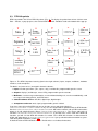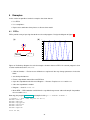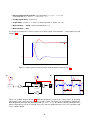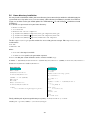
1
RTAI-Lab tutorial: Scilab, Comedi, and real-time control
Roberto Bucher 1
Simone Mannori
Thomas Netter 2
February 28, 2008
Summary
RTAI-Lab is a tool chain for real-time software and control system development. This tutorial shows how
to install the various components: the RTAI real-time Linux kernel, the Comedi interface for control and
measurement hardware, the Scilab/Scicos GUI-based CACSD modeling software and associated RTAI-Lab
blocks, and the xrtailab interactive oscilloscope. RTAI-Lab’s Scicos blocks are detailed and examples show
how to develop elementary block diagrams, automatically generate real-time executables, and add custom
elements.
1 Main
RTAI-Lab developer, person to contact for technical questions: roberto.bucher at supsi.ch, see page 46
of tutorial, person to contact for edits: tnetter at ifi.unizh.ch
Note: Because of frequent updates, this document may not be mirrored on any server apart from www.rtai.org
2 Author
Contents
1 Introduction
1.1 RTAI-Lab tool chain . . . . . . . . . . . . . . . . . . . . . . . . . . . . . . . . . . . . . . . . .
1.2 Commercial software . . . . . . . . . . . . . . . . . . . . . . . . . . . . . . . . . . . . . . . . .
2 Installation
2.1 Requirements . . . . . . . . . .
2.1.1 Hardware requirements
2.1.2 Software requirements .
2.2 Mesa library . . . . . . . . . . .
2.3 EFLTK library . . . . . . . . . .
2.4 Linux kernel and RTAI patch . .
2.5 Comedilib . . . . . . . . . . . .
2.6 RTAI (1st pass) . . . . . . . . .
2.7 RTAI tests . . . . . . . . . . . .
2.8 Comedi . . . . . . . . . . . . .
2.9 RTAI (2nd pass) . . . . . . . .
2.10 Scilab/Scicos . . . . . . . . . .
2.11 RTAI-Lab add-ons to Scilab . .
2.12 User configuration . . . . . . .
2.13 Load the modules . . . . . . .
4
4
4
.
.
.
.
.
.
.
.
.
.
.
.
.
.
.
.
.
.
.
.
.
.
.
.
.
.
.
.
.
.
.
.
.
.
.
.
.
.
.
.
.
.
.
.
.
.
.
.
.
.
.
.
.
.
.
.
.
.
.
.
.
.
.
.
.
.
.
.
.
.
.
.
.
.
.
.
.
.
.
.
.
.
.
.
.
.
.
.
.
.
.
.
.
.
.
.
.
.
.
.
.
.
.
.
.
.
.
.
.
.
.
.
.
.
.
.
.
.
.
.
.
.
.
.
.
.
.
.
.
.
.
.
.
.
.
.
.
.
.
.
.
.
.
.
.
.
.
.
.
.
.
.
.
.
.
.
.
.
.
.
.
.
.
.
.
.
.
.
.
.
.
.
.
.
.
.
.
.
.
.
.
.
.
.
.
.
.
.
.
.
.
.
.
.
.
.
.
.
.
.
.
.
.
.
.
.
.
.
.
.
.
.
.
.
.
.
.
.
.
.
.
.
.
.
.
.
.
.
.
.
.
.
.
.
.
.
.
.
.
.
.
.
.
.
.
.
.
.
.
.
.
.
.
.
.
.
.
.
.
.
.
.
.
.
.
.
.
.
.
.
.
.
.
.
.
.
.
.
.
.
.
.
.
.
.
.
.
.
.
.
.
.
.
.
.
.
.
.
.
.
.
.
.
.
.
.
.
.
.
.
.
.
.
.
.
.
.
.
.
.
.
.
.
.
.
.
.
.
.
.
.
.
.
.
.
.
.
.
.
.
.
.
.
.
.
.
.
.
.
.
.
.
.
.
.
.
.
.
.
.
.
.
.
.
.
.
.
.
.
.
.
.
.
.
.
.
.
.
.
.
.
.
.
.
.
.
.
.
.
.
.
.
.
.
.
.
.
.
.
.
.
.
.
.
.
.
.
.
.
.
.
.
.
.
.
.
.
.
.
.
.
.
.
.
.
.
.
.
.
.
.
.
.
.
.
.
.
.
.
.
.
.
.
.
.
.
.
.
.
.
.
.
.
.
.
.
.
.
.
.
.
.
.
.
.
.
.
.
.
.
.
.
.
.
.
.
.
.
.
.
.
.
.
.
.
.
.
.
.
.
.
.
.
.
.
.
.
.
.
.
.
.
.
.
.
.
.
.
.
.
.
.
.
.
.
.
.
.
.
.
.
.
.
.
.
5
5
5
5
6
6
6
8
8
8
9
9
10
10
10
11
3 Development with RTAI-Lab
3.1 Boot Linux-RTAI . . . . . . . . .
3.2 Start Scicos . . . . . . . . . . . .
3.3 RTAI-Lib palette . . . . . . . . . .
3.4 Real-time sinewave: step by step
3.4.1 Create block diagram . .
3.4.2 Compile . . . . . . . . . .
3.4.3 Execute . . . . . . . . . .
3.4.4 Change parameters . . .
3.4.5 Stop executable . . . . .
.
.
.
.
.
.
.
.
.
.
.
.
.
.
.
.
.
.
.
.
.
.
.
.
.
.
.
.
.
.
.
.
.
.
.
.
.
.
.
.
.
.
.
.
.
.
.
.
.
.
.
.
.
.
.
.
.
.
.
.
.
.
.
.
.
.
.
.
.
.
.
.
.
.
.
.
.
.
.
.
.
.
.
.
.
.
.
.
.
.
.
.
.
.
.
.
.
.
.
.
.
.
.
.
.
.
.
.
.
.
.
.
.
.
.
.
.
.
.
.
.
.
.
.
.
.
.
.
.
.
.
.
.
.
.
.
.
.
.
.
.
.
.
.
.
.
.
.
.
.
.
.
.
.
.
.
.
.
.
.
.
.
.
.
.
.
.
.
.
.
.
.
.
.
.
.
.
.
.
.
.
.
.
.
.
.
.
.
.
.
.
.
.
.
.
.
.
.
.
.
.
.
.
.
.
.
.
.
.
.
.
.
.
.
.
.
.
.
.
.
.
.
.
.
.
.
.
.
.
.
.
.
.
.
.
.
.
.
.
.
.
.
.
.
.
.
.
.
.
.
.
.
.
.
.
.
.
.
.
.
.
.
.
.
.
.
.
.
.
.
.
.
.
.
.
.
.
.
.
.
.
.
.
.
.
.
.
.
.
.
.
.
.
.
.
.
.
.
.
.
.
.
.
.
.
.
12
12
12
13
15
15
16
18
19
19
4 Examples
4.1 FIFOs . . . . . . . . . . . . . . . . . . . . . .
4.2 Semaphores . . . . . . . . . . . . . . . . . .
4.3 From continuous- to discrete-time . . . . . . .
4.3.1 Discretize the system . . . . . . . . .
4.3.2 Block diagram and simulation . . . . .
4.3.3 Real-time model and simulation . . . .
4.4 DC Motor control . . . . . . . . . . . . . . . .
4.4.1 Motor position model . . . . . . . . . .
4.4.2 Digital model . . . . . . . . . . . . . .
4.4.3 Digital control . . . . . . . . . . . . . .
4.4.4 RTAI-Lab controller . . . . . . . . . . .
4.5 Hardware example: parallel port LED blinker
4.5.1 Parallel port + LED circuit . . . . . . .
4.5.2 C code for the parallel port device . .
.
.
.
.
.
.
.
.
.
.
.
.
.
.
.
.
.
.
.
.
.
.
.
.
.
.
.
.
.
.
.
.
.
.
.
.
.
.
.
.
.
.
.
.
.
.
.
.
.
.
.
.
.
.
.
.
.
.
.
.
.
.
.
.
.
.
.
.
.
.
.
.
.
.
.
.
.
.
.
.
.
.
.
.
.
.
.
.
.
.
.
.
.
.
.
.
.
.
.
.
.
.
.
.
.
.
.
.
.
.
.
.
.
.
.
.
.
.
.
.
.
.
.
.
.
.
.
.
.
.
.
.
.
.
.
.
.
.
.
.
.
.
.
.
.
.
.
.
.
.
.
.
.
.
.
.
.
.
.
.
.
.
.
.
.
.
.
.
.
.
.
.
.
.
.
.
.
.
.
.
.
.
.
.
.
.
.
.
.
.
.
.
.
.
.
.
.
.
.
.
.
.
.
.
.
.
.
.
.
.
.
.
.
.
.
.
.
.
.
.
.
.
.
.
.
.
.
.
.
.
.
.
.
.
.
.
.
.
.
.
.
.
.
.
.
.
.
.
.
.
.
.
.
.
.
.
.
.
.
.
.
.
.
.
.
.
.
.
.
.
.
.
.
.
.
.
.
.
.
.
.
.
.
.
.
.
.
.
.
.
.
.
.
.
.
.
.
.
.
.
.
.
.
.
.
.
.
.
.
.
.
.
.
.
.
.
.
.
.
.
.
.
.
.
.
.
.
.
.
.
.
.
.
.
.
.
.
.
.
.
.
.
.
.
.
.
.
.
.
.
.
.
.
.
.
.
.
.
.
.
.
.
.
.
.
.
.
.
.
.
.
.
.
.
.
.
.
.
21
21
22
25
25
25
27
28
28
28
29
30
33
33
33
5 Custom blocks
5.1 Overview of Scicos blocks . . . . . . . . . . . . .
5.2 Program a Scicos custom block . . . . . . . . . .
5.3 Generate a Scicos library of custom blocks . . .
5.4 Program the external C functions . . . . . . . . .
5.5 Compile your C functions and generate a library
5.6 Home directory installation . . . . . . . . . . . .
.
.
.
.
.
.
.
.
.
.
.
.
.
.
.
.
.
.
.
.
.
.
.
.
.
.
.
.
.
.
.
.
.
.
.
.
.
.
.
.
.
.
.
.
.
.
.
.
.
.
.
.
.
.
.
.
.
.
.
.
.
.
.
.
.
.
.
.
.
.
.
.
.
.
.
.
.
.
.
.
.
.
.
.
.
.
.
.
.
.
.
.
.
.
.
.
.
.
.
.
.
.
.
.
.
.
.
.
.
.
.
.
.
.
.
.
.
.
.
.
.
.
.
.
.
.
.
.
.
.
.
.
.
.
.
.
.
.
.
.
.
.
.
.
.
.
.
.
.
.
35
35
36
38
38
38
39
2
5.7
5.8
5.9
5.10
System-wide installation . . .
Use the block . . . . . . . . .
Create a Scicos palette . . .
Scicos C block data structure
.
.
.
.
.
.
.
.
.
.
.
.
40
40
40
41
A Notes on Linux configuration and installation
A.1 Kernel configuration . . . . . . . . . . . . . . . . . . . . . . . . . . . . . . . . . . . . . . . . .
A.2 Configuring the GRUB boot manager . . . . . . . . . . . . . . . . . . . . . . . . . . . . . . . .
A.3 udev and RTAI . . . . . . . . . . . . . . . . . . . . . . . . . . . . . . . . . . . . . . . . . . . .
42
42
43
44
B Reference: standard parallel port
44
References
45
C About this document / Bug reports
C.1 About the authors . . . . . . . .
C.2 Bug reports, suggestions . . . .
C.3 Software licenses . . . . . . . . .
C.4 Acknowledgements . . . . . . . .
.
.
.
.
.
.
.
.
.
.
.
.
.
.
.
.
.
.
.
.
.
.
.
.
.
.
.
.
.
.
.
.
.
.
.
.
.
.
.
.
.
.
.
.
.
.
.
.
.
.
.
.
.
.
.
.
D Useful files and links
.
.
.
.
.
.
.
.
.
.
.
.
.
.
.
.
.
.
.
.
.
.
.
.
.
.
.
.
.
.
.
.
.
.
.
.
.
.
.
.
.
.
.
.
.
.
.
.
.
.
.
.
.
.
.
.
.
.
.
.
.
.
.
.
.
.
.
.
.
.
.
.
.
.
.
.
.
.
.
.
.
.
.
.
.
.
.
.
.
.
.
.
.
.
.
.
.
.
.
.
.
.
.
.
.
.
.
.
.
.
.
.
.
.
.
.
.
.
.
.
.
.
.
.
.
.
.
.
.
.
.
.
.
.
.
.
.
.
.
.
.
.
.
.
.
.
.
.
.
.
.
.
.
.
.
.
.
.
.
.
.
.
.
.
.
.
.
.
.
.
.
.
.
.
.
.
.
.
.
.
.
.
.
.
.
.
.
.
.
.
.
.
.
.
.
.
.
.
.
.
.
.
.
.
.
.
.
.
.
.
.
.
46
46
46
46
46
47
3
1
Introduction
This tutorial shows how to install, use, and customize, a free1 , open-source, Computer Aided Control System
Design (CACSD) and real-time control tool-chain called RTAI-Lab.
Apart from being a tool to develop real-time control systems, RTAI-Lab also lets you integrate real-time
R
R
R
controllers and simulators generated by Mathworks’ Matlab
/Simulink
/Real-Time Workshop
and/or the
open source Scilab/Scicos/CodeGen CACSD software suite.
Furthermore, RTAI-Lab lets you:
• Develop and execute real-time software in a local/remote/distributed way,
• Monitor a controller’s local/remote/distributed execution,
• Change a controller’s parameters on the fly.
1.1
RTAI-Lab tool chain
The RTAI-Lab tool-chain is based on:
• Scilab/Scicos. Scilab is an open source CACSD software for numerical computation. Scilab includes
Scicos, a block diagram editor that can be used to create simulations and automatically generate and
compile code. See www.scilab.org and www.scicos.org
• Comedi. Comedi provides the drivers, library functions, and an API to interact with signal acquisition
hardware. Hundreds of devices are supported. See www.comedi.org
• RTAI. The Real-Time Application Interface (RTAI) is distributed as a package with a patch to apply
to the Linux kernel. RTAI inserts a sub-kernel where prioritized, hard real-time tasks can run. FIFOs
and shared memory can be used to transfer data between real-time and user space processes. See
www.rtai.org
• RTAI-Lib. RTAI-Lib is a palette of Scicos blocks that let you design block diagrams with sensors and
actuators. It provides an interface to RTAI and signal acquisition hardware. Block diagrams that use
RTAI-Lib can be compiled into RTAI execuatble software. It is included in the RTAI package.
• xrtailab. xrtailab is an oscilloscope-like software that can connect to your real-time executables. It
lets you visually monitor signals and real-time events using gauge, scope, and LED mock-ups. xrtailab
also lets you adjust parameters of the real-time executable while it runs. It is also part of RTAI.
1.2
Commercial software
All software used for RTAI-Lab is free and Open Source. The RTAI-Lab tool chain represents an alternative
to the commercial software listed below:
R
R
• Scilab/Scicos → Mathworks’ Matlab
/Simulink
• Comedi → drivers supplied by signal acquisition hardware vendors, but most vendors don’t supply
Linux drivers
R
R
R
R
R
• RTAI → LynxOS
from Lynuxworks
, MontaVista Linux
, QNX
, VxWorks
, etc.
R
• RTAI-Lib → Mathworks’ Real-Time Workshop
R
• xrtailab → LabView
Note that you can still use commercial software and use RTAI/RTAI-Lab as a target (see RTAI-TargetHOWTO and RTAI-UbuntuGutsy-Matlab in Appendix D). If you think you have sufficient funds to purchase
commercial software, you will then buy a better GUI, better documentation, support that you can pay for, and
the possibility to consult with the vendor in case of problems (especially if you work for a large company). On
the other hand, upgrades with bug fixes are expensive, should be budgeted, and included in your real-time
1 No
purchase cost. See licenses in Appendix C.3, page 46
4
software’s multi-year maintenance and extension plan. These costs represent a financial burden even for
companies with a few hundred employees and only a few licenses. The advantage of using exclusively Open
Source software in the RTAI-Lab tool chain is that you or a subcontractor can customize it. You probably
already know that. That’s why softwares that constitute the RTAI-Lab tool chain are developed.
2
Installation
The full installation requires several software packages to be downloaded from their development servers
and compiled from source. Since RTAI, RTAI-Lab, and Comedi are undergoing strong development we
recommend that you do not rely on precompiled packages provided by Linux distributions.
The following sections provide detailed instructions to install (order is important and must be followed).
If you are installing on an Ubuntu-based distribution you may also refer to www.rtai.org/RTAILAB/RTAIUbuntuGutsy-Matlab.txt
•
•
•
•
•
•
•
The Mesa 3D graphical library. http://www.mesa3d.org
The EFLTK graphic widgets library. equinox-project.org
A new Linux kernel that will be patched with RTAI code
The Comedilib data acquisition device interface library
The RTAI real-time modules
The Comedi data acquisition device modules
The Scilab/Scicos Computer Aided Control System Design (CACSD) software
Note: The next sections list commands where software minor versions are indicated with “x.x”. Make sure
to replace the “x” with version numbers that correspond to your downloads.
2.1
2.1.1
Requirements
Hardware requirements
Most PCs can run a Linux kernel patched with RTAI. Some hardware configurations deserve a specific
comment.
Comedi support. Before starting the installation, first check that your data acquisition card or external
hardware is supported by Comedi. See (this page may be out of date) http://www.comedi.org/hardware.html.
If you don’t see your hardware listed then download Comedi anyway (see section 2.5) and look/grep into
/usr/local/src/comedi/comedi/drivers
PCMCIA. Our PCMCIA card was not detected with some Linux kernels 2.6.13.xx, 2.6.14.xx, 2.6.19 (see
note in Sec. 2.4).
Laptops & PCI sharing. We have experienced incompatibilities with some Toshiba Satellite laptops. If
you use a data acquisition card that plugs into the PCMCIA/CardBus slot of a Toshiba Satellite laptop you
might see warning messages about PCI devices sharing the same IRQ when loading Comedi modules.
RTAI+Comedi might not work, but give it a try anyway. If you know of other laptops that have this problem,
or know how to solve the problem, please notify us.
A quick way to test whether your computer will easily work with RTAI is to download an ISO image from
issaris.homelinux.org/ takis/projects/rtai/livecd and conduct some latency tests. Note that failing to boot the
CD or run the tests does not necessarily mean your computer cannot run RTAI.
2.1.2
Software requirements
We assume that your Linux system is based on one of the available distributions such as Debian, Fedora,
Mandriva, Red Hat, Slackware, Suse, Ubuntu, etc., and that you have suitable software development libraries installed to compile a Linux kernel, as well as graphical development libraries.
Your working environment and list of packages should enable you to compile and install software as root.
Ensure that your distribution is up to date with the latest versions of development software such as
automake > 1.7, autoconf, libtool, bison, and doxygen.
Important: we recommend that gcc -v and g77 -v show a version lower than 4.0. For example gcc/g++/cpp
version 3.4.6 works. In the following, make sure your replace the version numbers that contain “x” with the
versions you downloaded!
5
2.2
Mesa library
Make a new installation of Mesa even if your distribution already includes it. Mesa is needed to compile
EFLTK. You will need development packages such as xlibs-dev,...,x11proto-xext-dev,...
1. Become root
2. cd /usr/local/src
3. Visit http://www.mesa3d.org or http://sourceforge.net/projects/mesa3d and download MesaLib6.x.x.tar.bz2
4. tar jxvf MesaLib-7.x.x.tar.bz2
5. cd Mesa-7.x.x
6. make realclean
7. make linux-x86 or make linux-x86-static
Note that linux-dri configurations are listed in the configs subdirectory.
See also http://dri.freedesktop.org/wiki/
8. make install
This queries whether to accept the default installation directories: /usr/local/include and /usr/local/lib.
Note that some Linux distributions may require installation in /usr/X11R6/include and /usr/X11R6/lib.
2.3
EFLTK library
EFLTK is needed by xrtailab. EFLTK is part of the EDE project ede.sourceforge.net. You will need packages gettext, flex, and svn.
1. cd /usr/local/src
svn co https://ede.svn.sourceforge.net/svnroot/ede/trunk/efltk
svn co https://ede.svn.sourceforge.net/svnroot/ede/trunk/ede
2. cd efltk
autoconf
./configure --disable-mysql --disable-unixODBC
./emake
./emake install
3. Edit /etc/ld.so.conf and add a line with the path /usr/local/lib on a line.
4. Execute /sbin/ldconfig to update the library database
2.4
Linux kernel and RTAI patch
• cd /usr/src
• Download RTAI (at least version 3.5) of either:
– Stable (numbered): http://www.rtai.org (e.g. rtai-3.3.tar.bz2)
tar xjvf rtai-3.3.tar.bz2
ln -s /usr/src/rtai-3.3 rtai
– Experimental (hot stuff, beware): cvs -d:pserver:[email protected]:/cvs/rtai co magma
(see also https://gna.org/cvs/?group=rtai )
• Check kernel version numbers of available RTAI patches:
ls /usr/src/rtai/base/arch/i386/patches/
and look for kernel version numbers in: hal-linux-<kernel-version>.patch
• Carefully read /usr/src/rtai/base/arch/i386/patches/README as it might request that you edit
some files after you have configured your kernel.
• Decide what kernel version you will use: 2.4.xx or a 2.6.xx
Note: If you use a PCMCIA card, we recommend kernels up to 2.6.12.6 or 2.6.17 and above. For kernels upwards
of 2.6.13.xx we have experienced “Oops” when inserting Comedi’s pcmcia module (including kernel 2.6.16.15).
2007-05-22: There have also been difficulties with some kernel 2.6.17.xx (2.6.17.4 is said to work, though) and
kernels ≥ 2.6.19. When compiling Comedi, one should therefore add the option --disable-pcmcia.
6
• Kernel 2.4.xx. The latest RTAI v.3.5 supports kernels 2.4.30 to 2.4.32 with ”hal-linux-2.4.xx-i386.patch”.
1. Download a ”vanilla” linux-2.4.x.tar.bz2 from http://www.kernel.org
2. Unpack the kernel: tar xjvf linux-2.4.30.tar.bz2
mv /usr/src/linux-2.4.30 /usr/src/linux-2.4.30-rtai
ln -s /usr/src/linux-2.4.30-rtai linux
3. Patch the kernel:
cd /usr/src/linux
patch -p1 < <rtaidir>/base/arch/i386/patches/<kernel-version>.patch
for example:
patch -p1 < /usr/src/rtai/base/arch/i386/patches/hal-linux-2.4.30-i386.patch
4. make xconfig or make menuconfig
5. Configure the kernel. See details in Appendix A.
6. Possibly do edits requested in /usr/src/rtai/base/arch/i386/patches/README
7. make
8. make modules install
9. make install
• Kernel 2.6.xx. The latest RTAI v.3.3 supports kernel 2.6.10 and upwards with ”hal-linux-2.6.xx-i386xxx.patch”
WARNING: Some Linux distributions include the new udev platform. That can induce problems if the
new inodes are not registered (see Section A.3).
1. Download a ”vanilla” linux-2.6.xx.xx.tar.bz2 from http://www.kernel.org
2. Unpack the kernel: tar xjvf linux-2.6.23.14.tar.bz2
mv /usr/src/linux-2.6.23.14 /usr/src/linux-2.6.23.14-rtai
ln -s /usr/src/linux-2.6.23.14-rtai linux
3. Patch the kernel:
cd /usr/src/linux
patch -p1 < <rtaidir>/base/arch/i386/patches/<kernel-version>.patch
for example:
patch -p1 < /usr/src/rtai/base/arch/i386/patches/hal-linux-2.6.23.14-i386-r12.patch
4. make xconfig or make menuconfig
5. Configure the kernel. See details in Appendix A
6. Possibly do edits requested in /usr/src/rtai/base/arch/i386/patches/README
7. make
8. make modules install
9. make install
• Update your boot loader (either lilo or grub):
– Lilo: edit /etc/lilo.conf, and execute lilo
– Grub: edit /boot/grub/menu.lst (Debian) or /etc/grub.conf (Fedora, see Appendix B)
• Add module names to /etc/modules (Debian), e.g. pcmcia if you use a laptop with a signal acquisition
card and execute update-modules (Debian)
• Reboot computer into newly compiled kernel
7
2.5
Comedilib
1. cd /usr/local/src
2. cvs -d :pserver:[email protected]:/cvs/comedi login
cvs -d :pserver:[email protected]:/cvs/comedi co comedi
cvs -d :pserver:[email protected]:/cvs/comedi co comedilib
3. cd comedilib
4. Read software installation requirements in README.CVS and verify that your packages (automake etc.)
are up to date with automake --version
5. sh autogen.sh
Note: you may ignore warnings and reminders
6. ./configure −−sysconfdir=/etc
Note: pay attention to warnings and possibly remedy to these by installing extra software/packages
7. make and make install
Note: installation places comedi.h and comedilib.h in /usr/local/include. You will later have to
overwrite these header files with those from Comedi (see Sec. 2.8).
8. make dev
This step creates the /dev/comedi[0-3] device inodes.
9. Optional calibration tool: comedi calibrate
Install packages from your favourite Linux distribution: libboost-program-options-dev and libgsl0-dev
See also RTAI manual Sec. 4.7-8.
2.6
RTAI (1st pass)
This is usually straightforward. For more details download a draft of the RTAI User Manual Racciu and
Mantegazza [2006]. You will need packages libxmu-dev and libxi-dev.
1. cd /usr/src/rtai)
2. make xconfig or make menuconfig
3. Menu General: verify default directories:
• Installation directory /usr/realtime
• Kernel source directory /usr/src/linux
4.
5.
6.
7.
8.
2.7
Menu General: optionally select RTAI Documentation (HTML, PDF,...)
Menu Machine (x86): adjust Number of CPUs (default = 2)
Exit xconfig/menuconfig and save configuration
make and make install
IMPORTANT: Add /usr/realtime/bin to the PATH variable in /etc/profile or your home directory’s
.bashrc.
RTAI tests
Load RTAI-related modules (Section 2.13, insmod modules rtai hal to rtai fifos). You should measure
your system’s latency to real-time interrupts:
cd /usr/realtime/testsuite/kern/latency
./run
This launches a periodic task. The default period of 100000 ns is defined by DEFAULT PERIOD in
/usr/src/rtai/testsuite/kern/latency/latency-module.c and can be redefined upon module insertion
(see below). Watch lat min (ns) and overruns. Load your computer’s CPU, e.g. use multimedia applications.
If overruns becomes greater than zero then you might try to lenghten the period:
• Type ctrl-c to stop execution
• insmod modules of Section 2.13 from rtai hal.ko to rtai fifos.ko
8
• insmod /usr/realtime/modules/rtai lxrt.ko
insmod latency rt.ko period=1000000
./display
Overruns should either remain at zero or increase much more slowly. If they are still increasing then
stop execution and reload latency rt.ko with a longer period.
Stop execution: ctrl-c
rmmod latency rt
You may compare your latency results with those published at issaris.org/˜ takis/projects/rtai → Benchmarks.
2.8
Comedi
In case of difficulties, please refer to the INSTALL file in the comedi directory and to the documentation at
www.comedi.org.
IMPORTANT: Make any edits that may be requested in /usr/src/rtai/base/arch/i386/patches/README,
especially if they apply to the Linux kernel’s .config because it is read by Comedi’s configure script. See
also earlier note in Sec. 2.4 if you use a PCMCIA card.
1. cd /usr/local/src/comedi
2. sh autogen.sh
3. ./configure or possibly:
./configure --with-linuxdir=/usr/src/linux --with-rtaidir=/usr/realtime
or: ./configure --with-linuxdir=/usr/src/linux --with-rtaidir=/usr/realtime --enable-kbuild
with PCMCIA acquisition card: ./configure --with-linuxdir=/usr/src/linux --with-rtaidir=/usr/realtime
--enable-pcmcia
Note: Towards the end of the output pay attention that either CONFIG IPIPE, CONFIG RTHAL, or
CONFIG ADEOS is set to “yes”. This reflects what is set in /usr/src/linux/.config
4. make
5. make install (installs the comedi kernel modules)
6. make dev
7. cp include/linux/comedi.h include/linux/comedilib.h /usr/include/
cp include/linux/comedi.h include/linux/comedilib.h /usr/local/include/
8. ln -s /usr/include/comedi.h /usr/include/linux/comedi.h
ln -s /usr/include/comedilib.h /usr/include/linux/comedilib.h
9. Load RTAI and Comedi modules (Section 2.13)
10. Configure Comedi to work with you data acquisition hardware (section 2 of Comedi documentation
www.comedi.org/doc). The Comedi manual and man comedi config show how to associate a particular driver and hardware device to one of the /dev/comedi device files. For example, to configure a
National Instruments 6024E PCMCIA card, type:
comedi config -v /dev/comedi0 ni mio cs
and the output is:
configuring driver=ni mio cs 0,0,0,0,0,0,0,0,0,0,0,0,0,0,0,0,0,0,0,0,0,0,0,0,0,0,0,0,0,0,0,0,
WARNING: with the new udev platform there are some problems if the new inodes are not registered
(see Section A.3).
2.9
RTAI (2nd pass)
1. cd /usr/src/rtai
2. make xconfig or make menuconfig
3. Menu Add-ons:
• Select COMEDI support over LXRT
• Specify COMEDI installation directory (/usr/local or /usr). The directory should contain
lib/libcomedi.a, include/comedi.h and include/comedilib.h
9
4. Menu RTAI Lab:
• Select RTAI Lab
• Adjust EFLTK installation directory (default is /usr/local)
5. Exit xconfig/menuconfig and save configuration
6. make and make install
2.10
1.
2.
3.
4.
5.
6.
7.
8.
9.
10.
2.11
1.
2.
3.
4.
5.
6.
2.12
Scilab/Scicos
cd /usr/local
Download the latest version of Scilab source code from www.scilab.org
It sometimes happens that the latest version requires a patch to be downloaded. Check www.scicos.org
tar xzvf scilab-4.x.x-src.tar.gz
Ensure that your Linux system has the following packages installed: g77, sablotron, tcl8.4-dev, tk8.4dev, xaw3dg, xaw3dg-dev, libpvm3, pvm-dev, and optionally the set of development packages associated with gtk-2.0.
cd scilab-4.x.x
Depending on your Linux distribution you may try either:
./configure
Debian:
./configure --without-java --with-tcl-library=/usr/lib --with-tcl-include=/usr/include/tcl8.4
Fedora Core: ./configure --without-java
make all
Note: DO NOT make install
ln -s /usr/local/scilab-4.x.x/bin/scilab /usr/local/bin/scilab
In a terminal, as normal user, type: scilab. Then type quit at Scilab’s prompt. If Scilab did not start,
see end of Section 2.12.
RTAI-Lab add-ons to Scilab
cd /usr/local
Download the files for Scilab-4.1.2 from web.dti.supsi.ch/ bucher/scilab.html
tar zxvf scilab-4.1.2-rtailab.tgz
cd scilab-4.1.2-rtailab/macros
make install
exit and then, as normal user: make user
User configuration
Every RTAI-Lab user must edit ${HOME}/.Scilab/scilab-4.x.x/.scilab with:
load(’SCI/macros/RTAI/lib’)
%scicos_menu($+1)=[’RTAI’,’RTAI CodeGen’,’Set Target’]
scicos_pal($+1,:)=[’RTAI-Lib’,’SCI/macros/RTAI/RTAI-Lib.cosf’]
These lines add:
• Menu RTAI to the Scicos diagram editor with items →CodeGen and →Set Target
• Palette RTAI-Lib to menu Edit→Palettes
To add Scilab to the executable path you must either:
cd /usr/local/bin
ln -s /usr/local/scilab-4.x.x/bin/scilab scilab
or add /usr/local/src/scilab-4.x.x/bin to the PATH variable in your .bash profile and/or .bashrc
or relevant shell start-up file.
10
2.13
Load the modules
To compile and execute real-time RTAI-Lab programs you must boot the Linux-RTAI kernel. If all goes well
your acquisition hardware will be detected (try cardctl info for kernels less that 2.6.13 or pccardctl info
otherwise). You then load RTAI- and hardware-related modules. Note that which modules to load depends
on your RTAI kernel configuration.
We recommend to initially load the modules manually, and possibly later configure your system to load these
modules at boot time using system files or commands (depending on your Linux distribution and hardware)
such as /etc/modules, update-modules, /etc/modutils/..., /etc/hotplug/ or /etc/udev and/or a
manually launched script.
To manually load the modules, you will have to be root or use sudo. You can check the progress by issuing
dmesg commands or tail -f /var/log/messages. For example, on a laptop with a National Instruments
DAQCard-6024E PCMCIA card (see hardware-specific comments indicated by # signs below), here’s how
to load the modules:
modprobe rsrc_nonstatic
# PCMCIA-related
modprobe i82092
# PCMCIA-related
modprobe yenta_socket
# PCMCIA-related
insmod /usr/realtime/modules/rtai_hal.ko
insmod /usr/realtime/modules/rtai_up.ko
# or rtai_lxrt.ko
insmod /usr/realtime/modules/rtai_fifos.ko
insmod /usr/realtime/modules/rtai_sem.ko
insmod /usr/realtime/modules/rtai_mbx.ko
insmod /usr/realtime/modules/rtai_msg.ko
insmod /usr/realtime/modules/rtai_netrpc.ko ThisNode="127.0.0.1"
insmod /usr/realtime/modules/rtai_shm.ko
insmod /usr/realtime/modules/rtai_signal.ko
insmod /usr/realtime/modules/rtai_tasklets.ko
modprobe comedi
modprobe kcomedilib
modprobe comedi_fc
modprobe 8255
# acq. card hardware-specific
modprobe ni_mio_cs
# acq. card hardware-specific
insmod /usr/realtime/modules/rtai_comedi.ko
/etc/init.d/pcmciautils restart
# from pcmciautils package
# or pcmcia restart (kernel < 2.6.13)
Note that you may have to load more modules in /usr/realtime/modules/ depending on what blocks you
use in your application. It may be useful to write a shell script to load these modules after you boot RTAI.
11
3
Development with RTAI-Lab
Real-time software development with the RTAI-Lab tool chain is done with the Scilab/Scicos block diagram
editor and associated palettes of blocks, including the RTAI-Lib palette.. Some testing of the real-time
executable can be done with xrtailab. New Scicos blocks may be programmed using the Scilab language,
and their executable component programmed in C (see section 5).
Scicos window with RTAI menu
Figure 1: Scilab, Scicos, and 2 palettes (Sources and RTAI-Lib). Note the addition of the RTAI drop-down
menu button to the standard Scicos window. The most important block in the Sources palette is the red
clock.
3.1
Boot Linux-RTAI
Boot Linux-RTAI. Load associated modules (section 2.13).
3.2
Start Scicos
To launch Scilab, type at a shell’s command prompt: scilab
At Scilab’s prompt type: scicos
This opens the Scicos window in which you will draw block diagrams. For a tutorial on Scicos check
http://www.scicos.org/TUTORIAL/tutorial.html
RTAI-Lab modifies 2 aspects of Scicos (Fig.1):
• There is an RTAI menu towards the right of the Scicos window
• There is an RTAI-Lib palette
12
3.3
RTAI-Lib palette
RTAI-Lab provides the Scicos RTAI-Lib palette (Fig. 2). To display the palette from Scicos click on menu
Edit → Palettes, a pop-up opens, then click on RTAI-Lib which should be listed at the bottom of the pop-up.
Sine
Scope
SCOPE
Mbx Send Ovw
MBX1
Square
Meter
METER
Mbx Rcv no blk
MBX1
Step
Led
LED
extdata
test.dat
SENSOR
SENS
ACTUATOR
ACT
COMEDI A/D
comedi0 CH−0
SEM wait
SEM1
COMEDI D/A
comedi0 CH−0
SEM signal
SEM1
Mbx Send if
MBX1
COMEDI DI
comedi0 CH−0
C RTAI
Block
Mbx rcv blk
MBX1
COMEDI DO
comedi0 CH−0
Fifoout
0
Fifoin
0
Figure 2: The RTAI-Lib palette featuring (from left to right columns) inputs, outputs, mailboxes, hardware
interfaces, and semaphores.
The blocks are (more or less) arranged in thematic columns:
1. Inputs: function generators (sine, square, step), read data file, programmable generic sensor
2. Outputs: displays (oscilloscope, meter, LED), programmable generic actuator
3. Mailboxes: send message and overwrite, receive without blocking task, receive unconditionally, send
message if task timing permits, and FIFO boxes
4. Comedi hardware drivers: A/D, D/A, digital input, digital output
5. Semaphores and more: wait, signal, programmable generic C block
If you have correctly installed RTAI-Lab you can find the source code for the blocks in
/usr/local/scilab-4.x.x/macros/RTAI. In any case the original blocks provided with the RTAI distribution are in /usr/src/rtai/rtai-lab/scilab/macros/RTAI. Most of these blocks call up RTAI-Lab functions
written in C and compiled into the library /usr/realtime/lib/libsciblk.a. The source code of the C
functions is in /usr/src/rtai/rtai-lab/scilab/devices. If you look at the source code of the RTAI-Lab
functions, you will see how RTAI API functions are called. These RTAI API functions are documented in
HTML and other formats in /usr/src/rtai/doc/generated if you specified that documentation be generated during RTAI installation (section 2.6).
A detailed review of RTAI-Lib blocks follows. Default values are indicated in brackets.
13
1. Inputs:
• Sine. Real-time sinewave generator. The Sine block lets you adjust amplitude [1], frequency
[1] (Hz), phase [0], bias [0], and delay [0]. Furthermore, you can adjust these parameters from
xrtailab or an external program while the real-time executable is running.
• Square. Real-time square waveform. The Square block lets you adjust amplitude [1], period [4] (s), pulse width [2] (s), bias [0], and delay [0] (s). You can also adjust parameters from
xrtailab or other programs during real-time execution.
• Step. Step function. The Step block lets you adjust amplitude [1] and delay [0] (s).
• extdata. Load data from a file. The file [test.dat] must contain a single column with ASCII values
at each sampling time [1000 points].
• SENSOR. Generic sensor input. You can adjust the number of outputs [1] and an identifier [SENS].
Following that another dialog box opens where you can enter C code. This code is compiled and
linked after clicking on OK. Although the dialog box has basic editing functions similar to Emacs,
we recommend that you edit your code in a separate editor and then copy-paste it into the dialox
box.
2. Outputs:
Scope, Meter, and LED are output blocks that send data to xrtailab displays.
• Scope. xrtailab multichannel oscilloscope. You can adjust the number of inputs [1] and the
scope’s name [SCOPE].
• Meter. xrtailab single channel meter. You can adjust the meter’s name [METER].
• LED. xrtailab multichannel multi-LED block. Each LED switches ON if the input is positive. You
can adjust the number of inputs/LEDs [1] and the LED block’s name [LED].
• ACTUATOR. Generic actuator output. This block is similar to the SENSOR block. You can adjust
the number of inputs [1] and an identifier [ACT].
3. Mailboxes:
Mailboxes let real-time tasks exchange arbitrarily-seized messages. Their advantage is that there
is no need to size mailbox buffers to cater for unusually large messages. Message passing may
be interrupted by real-time constraints. See /usr/src/rtai/doc/generated/html/api/group mbx.html and
[Sarolahti, 2001]
Local task blocking may occur when exchanging a packet between a local host and a mailbox on a
remote host. Furthermore, packet transmission to a mailbox on a remote host is currently limited by
the UDP packet size (≈ 1500 bytes).
• Mbx Send Ovw. Sends a message to a mailbox, possibly overwriting what is already in the mailbox. You can adjust the number of message input ports [1], mailbox name [MBX], and mailbox IP
address [127.0.0.1] (localhost). See also RTAI API documentation for function rt mbx ovrwr send.
• Mbx Rcv no blk. Receives a message only if the whole message can be passed without blocking
the calling task. However, if the mailbox is on a remote host, the calling task may be blocked. You
can adjust the number of message output ports [1], mailbox name [MBX], and mailbox IP address
[127.0.0.1] (localhost). See also RTAI API documentation for function rt mbx receive if.
• Mbx Rcv blk. Receives a message. The calling task will be blocked until all bytes of the message arrive or an error occurs. You can adjust the number of message output ports [1], mailbox
name [MBX], and mailbox IP address [127.0.0.1] (localhost). See also RTAI API documentation
for function rt mbx receive.
• Mbx Send if. Sends a message only if the whole message can be passed without blocking the
calling task. However, if the mailbox is on a remote host, the calling task may be blocked. You
can adjust the number of message input ports [1], mailbox name [MBX], and mailbox IP address
[127.0.0.1] (localhost). See also RTAI API documentation for function rt mbx send if.
• FIFOout and FIFOin. Multichannel FIFO. You can adjust the number of inputs [1], the FIFO’s
number [0], and the FIFO’s Dimension [50000] (in bytes).
14
4. Comedi hardware drivers:
• Comedi A/D. Comedi supported Analog Input. You can select your acquisition card’s analog
input channel [0], the device if you have several acquisition cards [comedi0], the range number as
specified in your acquisition hardware’s manual [0] (warning: the value to enter is not expressed
in volts), and the type of voltage reference [0], e.g. nonreferenced single ended, referenced single
ended, and differential. See also Comedi API comedi data read.
• Comedi D/A. Comedi supported Analog Output. The parameters are similar to Comedi A/D. See
also Comedi API comedi data write.
• Comedi DI. Comedi supported Digital Input. You can select the channel [0] and device [comedi0].
See also Comedi API comedi dio read.
• Comedi DO. Comedi supported Digital Output. You can select the channel [0], device [comedi0],
and threshold [1]. If the data input to the block is greater than the threshold value, then a single
bit will be output by your hardware. See also Comedi API comedi dio write.
5. Semaphores and more:
Semaphores can be used to synchronize real-time tasks. Similarly to mailboxes, caution is needed
with respect to blocking when exchanging a semaphore between a local and a remote host.
• SEM wait. Decrement a semaphore’s value and wait for a signal event. The caller task is blocked
and queued up as long as the semaphore’s value is negative. You can adjust the semaphore’s
name [SEM] and IP address [127.0.0.1] (localhost). See also RTAI API documentation for function
rt sem wait.
• SEM signal. Increment a semaphore’s value. If the resulting value is not positive then the first
task in the semaphore’s waiting queue is allowed to run. You can adjust the semaphore’s name
[SEM] and IP address [127.0.0.1] (localhost). See also RTAI API documentation for function
rt sem signal.
• C RTAI. This is a generic block that lets you edit C code. It is based on Scilab’s C-Block2 found
in the “Others” palette. When you click on the C RTAI Block a dialog window opens where you
can edit block parameters such as the name of the main function that it will contain, the number
of inputs and outputs for data and events, and various parameters (see section 5.10 and also
[Campbell, Chancelier, and Nikoukhah, 2006], section 9.5). After clicking on OK a second window
opens with a code skeleton to edit. It is best to copy-paste code from your favorite editor into this
window. When you click on OK the code is compiled and linked. If your code is relatively large
we recommend that you program your own block instead of using C RTAI Block (see section 5).
3.4
Real-time sinewave: step by step
In this example you use Scilab/Scicos to draw a block diagram that generates a sinewave. You automatically generate and compile a real-time executable. You test the program and visualize the sinewave with
xrtailab.
3.4.1
Create block diagram
Let’s create the preliminary Sinewave diagram shown in figure 3.
Select palettes. Start Scicos. Open the Sources palette: click on menu Edit → Palettes and select Sources
at the top of the pop-up window. Open the RTAI-Lib palette in a similar way (figure 1).
Keyboard shortcuts. Note that by default, Scicos has a few customizable keyboard shortcuts, list them
with menu Misc → Shortcuts.
Select blocks. From the Sources palette, left-click on the red clock. Move your mouse to the main Scicos
window. You should see the block’s contour being dragged as your mouse cursor enters the main Scicos
window. Left-click again to place the clock in the main Scicos window, somewhere towards the upper center
of the window. You may also right-click to cancel block placement during the drag.
From the RTAI-Lib palette, left-click on the Sine block and place it towards the lower left of the main Scicos
window. Place also a Scope block towards the lower right.
Align blocks. Scicos does not currently feature a block placement grid so blocks are not perfectly aligned
to make a nice diagram. Two methods can help block alignment:
15
Figure 3: Preliminary RTAI-Lib block diagram with real-time sinewave generator and xrtailab scope blocks.
• Use Scicos’s Align function: menu Edit → Align. Click on the Sine block’s data output port (the black
triangle to the right of the block) and then on the Scope’s data input port. One of the blocks will then
be shifted so that both blocks’ ports are aligned. A faster way to align blocks using keyboard shortcuts
is to place the mouse over a block’s port (input or output), then use keyboard shortcut “a”, then click
on the port of the block to be aligned.
• Adjust mouse acceleration so that motion increments are more discretized: type xset m 4 1 in a
terminal/shell window. The drawback is that your mouse might move too fast for comfort.
Link blocks. Menu Edit → Link. Click on Sine’s output port. Click on Scope’s input port. A link is drawn
from Sine to Scope. Click on the clock’s event output port (the red triangle below the clock). Then draw an
S-shaped link to the Sine block by clicking below the clock’s port, once more above the Sine’s event port,
and finally directly onto the Sine’s event port. A red link is drawn from the clock to the Sine. Draw another
event link by clicking onto the red line, then click above the Scope, and click again onto the Scope’s event
port.
Set block parameters. Click on the clock. You may adjust period and initialization times (values are in
seconds). Click on Sine, adjust parameters accordingly, then click on OK. You may also edit the Scope’s
name and notice that it may actually have more than one data input. In any case, it is necessary that Scicos
evaluate all blocks. This is done when you click on a block, adjust its parameters, and then click on OK. A
general way to have all blocks evaluated is to select menu Simulate → Eval. You must do this Eval operation
every time you add a block to a diagram and omit inspecting its internal parameters.
Create super block. Menu Diagram → Region to Super Block. You must draw an elastic frame around the
Sine and Scope blocks, excluding the Clock (figure 4, left). First click above-left of the Sine block, then click
again below-right of the Scope block. The region then becomes a Super Block (Fig. 4, right).
3.4.2
Compile
Set target. You may optionally click on menu RTAI → Set Target and then click on the Super Block to
compile. A dialog box opens where you may modify:
• Target. This is the Makefile’s basename. See description below.
• Ode function. This is one of the ordinary differential equation functions available in Scilab. The default
is ode4. Possible values are:
– ode1. Uses Euler’s method (RK1)
– ode2. Uses Heun’s method (RK2), also known as the Improved Euler method.
– ode4. Uses a 4th order Runge-Kutta formula (RK4).
16
Figure 4: Left: preliminary RTAI-Lib block diagram during Region to Super Block framing. All blocks except
the clock should be contained in the region. Right: resulting Super Block.
The source code for these functions is available in $SCILAB/macros/RTAI/RTAICodeGen .sci. Scilab’s
ODE functions are detailed in section 3.2 of [Campbell et al., 2006] and also in [Sallet, 2004].
• Step between sampling. Indicates the number of computational sub-sampling points used for various
functions such as ODE functions. The default is 10.
(a)
(c)
(b)
Figure 5: Block diagram: code generation and compilation. (a): Scicos window after code generation. (b):
Dialog box to adjust generated filenames, makefile, and clock period. (c): Text output after compilation.
Compile block diagram. Menu RTAI → RTAI CodeGen. Then click on the Super Block. At this point Scilab
converts your block diagram into C code. For each block inside the Super Block two lines are output in the
Scicos window (Fig. 5a):
shared archive loaded
Link done
A dialog then opens (Fig. 5b shows the dialog with default values) where you may modify:
• New block’s name. This will be the name of the final executable. It will be saved in what Scilab thinks
is your current directory. The default is Untitled.
17
• Created files Path. This is the directory where the generated C files are saved along with a Makefile.
This is also the directory where compilation occurs.
• Target. This is the Makefile’s basename. It will be copied to the generated files directory and used for
compilation. The default value rtai corresponds to the file $SCILAB/macros/RTAI/RT templates/rtai.mak
• Sampling Time. This corresponds to the Period value set in the Clock block parameters, i.e. you can
adjust the clock here.
Click on OK and the compilation starts. Steps in the compilation can be monitored in the Scilab window (Fig.
5c). In case the compilation fails (this can happen for example when you develop your own custom blocks,
see section 5.2), you can still start the compilation manually by typing make in the directory where C files
were generated. This provides more debugging output that what is printed in the Scilab window.
If you kept the default values you should find an executable file called Untitled in your current directory.
3.4.3
Execute
Open two terminal shells.
Real-time executable. In the first terminal type: Untitled -u
This provides usage instructions as a list of command line options.
To start the real-time executable with verbose output type: Untitled -v
xrtailab. Note that xrtailab only executes when an RTAI Linux kernel is running. xrtailab will generate a
segmentation fault if started over a standard Linux kernel.
In the second terminal type:
xrtailab -h
xrtailab
Select menu File → Connect. . . (keyboard shortcut: alt-c) then Click on OK (Fig. 6).
Figure 6: xrtailab’s connect dialog box.
IP Address is that of the host where the real-time task is executing.
Identifiers IFTASK, RTS, RTL, RTE, RTM, and RTY are predefined in
rtmain.c, in the directory that contains the generated source code. If
several real-time tasks must run in parallel, a real-time task’s identifiers
may be set via the command line options (execute the task with option
-u to list command line options) and by adjusting values in the “Connect
to Target” dialog. Note that you may even edit rtmain.c to change the
real time task’s predefined identifiers.
xrtailab’s row of buttons (Fig. 7) lets you start and stop the real-time executable and open various displays
such as scopes, meters, and LEDs. At the time this tutorial is written, not all buttons are fully functional.
Some may find it more convenient to use the View menu and associated keyboard shortcuts.
Open a scope manager window by either clicking on the Scope button or selecting it in the View menu
(shortcut: alt-s). Then click on the Show/Hide checkbox to display the scope. You should see a 1 Hz
sinewave snaking smoothly in the scope.
Note that the Scope Manager lets you modify display properties such as the number of grid division (Sec/Div), colors, and filename. You can save data points (default: 1000) to a file (default filename: SCOPE).
You may also pause the display. Each trace’s properties can also be adjusted via the Trace tab. The trace
can be hidden, its offset shifted, and its color changed. You may also adjust the number of units per vertical
division.
18
ui
t
o
(w n
ithne
C proct
o
(w n file
ithne )
D out cpt
is ro
co fil
Sa nn e)
ve ect
D pro
el
e file
St te P
ar r
t o
St RT file
op c
o
Pa RT de
ra co
Sc me de
op ter
Lo e s
g
LE
D
M s
et
e
Sy r
nc
Te
xt
ed
ito
r
C
Q
Figure 7: xrtailab with scope manager window and a scope displaying a 1 Hz sinewave. Most functions of
the row of buttons are duplicated in the drop-down menus. Keyboard shortcuts are also available.
3.4.4
Change parameters
xrtailab lets you change “on the fly” the parameters that were defined in the Scicos block diagram. For
example, the Sine block has 5 parameters: amplitude (Value[0]), frequency (Value[1]), phase (Value[2]),
bias (Value[3]), and delay (Value[4]).
Click on the Parameters button. The Parameters Manager window opens. You might have to resize
xrtailab’s window and reposition the Parameters Manager window to obtain a convenient layout similar
to that shown in figure 8. Change Value[0] to 3 and press the Enter key. The sinewave’s amplitude will
increase accordingly. Change Value[1] to 2. This will double the sinewave’s frequency to 2 Hz and you will
notice that the wave lost its smoothness. This is an undersampling effect induced by the fact that the clock’s
period, as defined in the Scicos block diagram, is only of 0.1 s or 10 Hz.
Note that the Parameters Manager also lets you download block parameters from real-time tasks running
on remote hosts and upload them back after modification.
3.4.5
Stop executable
Click on the Stop hexagonal icon to disconnect xrtailab from the real-time target and terminate it. Note
that it is possible to only disconnect xrtailab from a target (alt-d) and leave it running. You can re-connect
to it later. Finally, you may also interrupt the real-time executable directly at the terminal where you launched
its execution: type ctrl-c.
19
Figure 8: xrtailab with Parameters Manager window. Parameters that have been changed are sinewave
amplitude (Value[0]) from 1 to 3 and frequency (Value[1]) from 1 to 2 Hz. The scope reveals an undersampled sinewave that results from the real-time executable’s clock being set to only 10 Hz.
20
4
Examples
In this section we provide a few basic examples that show how to:
• Use FIFOs
• Use semaphores
• Represent a continuous-time plant as a discrete-time model
4.1
FIFOs
FIFOs provide a way of passing data to other tasks and programs. Design the diagram of figure 9a.
(a)
(b)
1.0
0.8
0.6
0.4
0.2
0.0
−0.2
Sine
Fifoout
0
−0.4
−0.6
−0.8
−1.0
37.0
37.5
38.0
38.5
39.0
39.5
40.0
40.5
41.0
41.5
42.0
42.5
Figure 9: Preliminary diagram of a task that outputs sinewave data to a FIFO. An external program is then
used to read the data from /def/rtf0
• Click on Simulate → Eval to ensure all blocks are registered. You may change parameters in the Sine
block.
• Set clock period to 0.01
• Frame a Superblock around Sine and FIFOout
• Open the Superblock and click menu Diagram → Rename. Replace Untitled with fifo1
• Close the Superblock’s window
• Diagram → Save As: fifo1.cos
• Menu RTAI → RTAI CodeGen and click on the superblock to generate code and compile it to produce
the executable fifo1
Now copy the program readfifo.c and compile it with: gcc -o readfifo readfifo.c
/* readfifo.c -- Read a FIFO and print its data */
#include <stdio.h>
#include <unistd.h>
#include <sys/types.h>
#include <sys/stat.h>
#include <fcntl.h>
#include <signal.h>
static int end;
21
struct data{
float t;
float u[1];
};
static void do_end(int dummy) { end = 1; }
int main (void)
{
int fifo;
struct data val;
if ((fifo = open("/dev/rtf0", O_RDONLY)) < 0) {
fprintf(stderr, "Error opening /dev/rtf0\n");
exit(1);
}
signal(SIGINT, do_end);
while (!end) {
read(fifo, &val, sizeof(val));
printf("%f\t%f\n", val.t, val.u[0]);
}
return 0;
}
• In a terminal type: ./fifo1 -v
• In a second terminal type: ./readfifo
Two columns of data should start printing. Interrupt the program by typing ctrl-c.
• In the second terminal now type: ./readfifo > fifo.dat
Interrupt the program after 3 to 10 seconds by typing ctrl-c.
• In Scicos, menu Diagram → Quit
• In Scilab’s scilex window, type “n” and then type at Scilab’s “-->” command prompt to produce the plot
in Fig. 9b:
-->x = read(’fifo.dat’, -1, 2);
-->plot(x(:,1), x(:,2))
4.2
Semaphores
Semaphores are used as a signalling method between tasks. Design the diagram of figure 10.
• Open the SEM signal block and ensure that IP addr is 127.0.0.1
• Open the SEM wait block and ensure that IP addr is 0
• Open the left LED block and call it LED1
• Frame a Superblock on the left side around blocks Sine, SEM signal, and LED. Frame a Superblock
on the right side around blocks SEM wait, LED, Sine, and Scope.
• Set each clock to a Period of 0.001
• Simulate → Eval
22
Sine
SEM signal
SEM
SEM wait
SEM
LED
LED
LED
LED1
Sine
Scope
SCOPE
Figure 10: Preliminary diagram of two tasks that use semaphores. Left: the signalling task uses a sinewave
to increment a semaphore. Right: the waiting task reads the semaphore and produces an output only when
the sinewave in the signalling task is positive.
• Open the left Superblock and Diagram → Rename it to semsig. Note: you might have to Diagram → Replot to recenter the diagram. Warning: do not put a dash “-” in the name of a block,
RTAI CodeGen has problems with that. Close the window.
• Put a name tag under the Superblock: Object → Identification, click on the left Superblock and set ID
to semsig
• Open the right Superblock and rename it to semwait. Close the window.
• Save the diagram to sem.cos
• RTAI → RTAI CodeGen the left Superblock
• RTAI → RTAI CodeGen the right Superblock
• In a terminal type: semsig -v -n IFTASL -d LED
• In a second terminal type: semwait -v -e
• In a third terminal type: xrtailab -v
• In xrtailab:
– Connect to semwait: type alt-c and set the “Led identifier” field to LED
– Open and display an LED: click on the light bulb button then check Show/Hide. The signalling
task’s LED should blink every second
– Open and display a scope. You should see the waiting task’s truncated sinewave scrolling in a
jerky manner every second (Fig.11).
– Disconnect from semwait: type alt-d
– Connect to semsig: type alt-c. In the Task Identifier field type: IFTASL and click on the OK button.
– Open and display an LED. LED1 should blink at 1 Hz.
– Open the “parameters manager”: type alt-p. Increase Value[1] of RPARAM[1] from 1 to 2 and
press Enter. By doing this you have increased semsig’s Sine frequency from 1 to 2 Hz. LED1
should now blink at 2 Hz.
– Disconnect from semsig: type alt-d
– Connect again to semwait: type alt-c. Set Task Identifier to IFTASK
– Open again an LED and a scope. The LED now blinks at 2 Hz and the sinewave has twice as
many kinks.
23
Figure 11: xrtailab scope display of the sinewave generated by the semwait Superblock (the waiting task).
The green LED reflects the state of the LED block in the semsig Superblock (the signalling task). The
waiting task operates only when the “SEM wait” semaphore is positive (light green LED). The result is a
jerky sinewave synchronized to the semsig task’s semaphore.
24
4.3
4.3.1
From continuous- to discrete-time
Discretize the system
Say a continuous-time feedback system includes a plant modeled by the transfer function:
G(s) =
20
.
s2 + 4s
Use Scilab to discretize the system with a sampling time of 1 ms.
-->s = poly(0,’s’);
-->G = [20/(s^2 + 4*s)]
G =
20
-----2
4s + s
-->Gc = syslin(’c’,G);
-->T = 0.001;
-->Gd = ss2tf(dscr(tf2ss(Gc),T))
Gd =
0.0000100 + 0.0000100z
-----------------------2
0.9960080 - 1.996008z + z
The system’s discrete-time transfer function is therefore:
G(z) = 10−6
4.3.2
z2
10z + 10
.
− 1.996z + 0.996
Block diagram and simulation
Replicate the block diagram of figure 12 (you will use palettes Sources, Sinks, Linear, and Branching).
num(z)
den(z)
2
Mux
−1
Figure 12: Scicos block diagram to simulate the step response of a discretized plant.
• Clock block: set Period = 0.001, Init time = 0
• Step block: set step time = 1, Initial value = 0, Final value = 1.
• Gain block: set gain to 2
25
• Discrete SISO transfer function: set numerator to: 0.00001 + 0.00001*z
set denominator to: 0.996008 - 1.996008*z + z^2
• Feedback gain block: set gain to -1
• Scope block: set Ymin = -1, Ymax = 3, Refresh period = 5, Buffer size = 20
• Menu Simulate → Setup: set Final integration time = 5
• Menu Simulate → Eval
Use Scicos to visualize the system’s response to a square signal: menu Simulate → Run produces the plot
of figure 13.
3
2
1
0
−1 +
0.0
0.5
1.0
1.5
2.0
2.5
3.0
3.5
4.0
4.5
5.0
Figure 13: Step response (dashed red line) of block diagram shown in Fig. 12
b)
a)
4
2
square wave
generator
2
num(z)
den(z)
0
Mux
−2
−1
−4 +
0
1
2
3
4
5
6
7
8
9
Figure 14: a) Block diagram of Fig. 12 modified to display the response to a square wave. b) Resulting
plot showing square wave and step response (red line). Note: This figure was assembled by exporting the
block diagram to Postscript and converting it with pstoedit -f fig. The plot was directly exported to Xfig
format. Both figures were then merged using Xfig and the numbering on the axes was enlarged using
Xfig’s “Update” button.
26
10
Modify the block diagram so as to simulate the response to a square wave input (Fig. 14a):
• Left clock: Period = 3, Init time = 0
• Square wave generator: Amplitude = 1
• Scope: Ymin = -4, Ymax = 4, Refresh period = 10, Buffer size = 20
• Menu Simulate → Eval generates Fig. 14b.
4.3.3
Real-time model and simulation
Modify again the block diagram using blocks from the RTAI-Lib palette (Fig. 14a):
• Replace the left clock and square wave generator with an RTAI-Lib Square block. Set Square block
parameters: Amplitude = 1, Period = 6, Impulse width = 3, Bias = 0, Delay = 0
• Replace the multiplexer and scope with an RTAI-Lib Scope block. Set input ports = 3
• Menu Diagram → Region to Super Block: frame all blocks except the clock. You then obtain Fig. 14b
• Open Super Block. Menu Diagram → Rename and set diagram name to rtex3. Close Super Block
window.
• Menu RTAI → RTAI CodeGen and compile
• In a terminal type: ./rtex3 -v
• In another terminal type: xrtailab
• In xrtailab: connect to target (alt-c), open the scope manager and show the scope. In the Scopes
Manager you can click on Trace tabs to adjust each trace’s color (Fig. 15).
Figure 15: xrtailab Scopes Manager and scope displaying real-time plots of the block diagram shown in
Fig. 14a
27
4.4
DC Motor control
In this example we show how to adapt a Simulink block diagram to Scicos and RTAI. This example is based
R
R
on the Control Tutorials for Matlab
and Simulink
, hosted at Carnegie Mellon University and University of
Michigan [Messner and Tilbury, 1998]: www.library.cmu.edu/ctms. Please refer to the “DC Motor position
modeling in Simulink” example. Sections 7.2 and 10.2 of [Campbell et al., 2006] also provide in-depth
information on using Scicos for control.
4.4.1
Motor position model
a)
b)
8
R
−
+
−
K
6
1/L
1/s
4
+
−
K
1/J
2
1/s
1/s
b
0 +
0.00
0.02
0.04
0.06
0.08
0.10
0.12
0.14
0.16
0.18
Figure 16: a) Continuous time model of DC motor position as described at www.library.cmu.edu/ctms.
b) Open-loop step response of DC motor.
• Replicate the model of Fig. 16a
• Menu Edit → Context: enter values for constants:
J = 3.2284E-6; b = 3.5077E-6; K = 0.0274;
R = 4; L = 2.75E-6
• Menu Simulate → Setup: Final integration time = 0.2
• Step block: Step time = 0, Initial value = 0, Final value = 1
• Clock block: Period = 0.001, Init time = 0
• Scope block: Ymin = 0, Ymax = 8, Refresh period = 0.2
• Menu Simulate → Eval
• Menu Simulate → Run: produces the plot of Fig. 16b
4.4.2
Digital model
• Menu Diagram → Region to Super Block: draw a frame around the computational blocks as shown in
Fig. 17a. You then obtain a superblock.
• Menu Diagram → Save As: save to dcmot-model.cos
• Menu Object → Get Info, then click on the superblock. A window opens, select “Others [Yes]” and
click on OK (Fig.17a). A second window opens, remember the superblock’s object number (here 43,
Fig. 17b) and click on OK
• Menu Diagram → Quit to exit Scicos, then type “n” to get past the junk in the Scilab window.
28
0.20
a)
b)
Figure 17: How to obtain information about a superblock prior to its discretization: menu Object → Get Info
then a) select Others [Yes] and b) remember block’s object number (43)
• In Scilab type:
(replace the “43” in the 3rd line with your superblock’s object number):
load dcmot-model.cos
J = 3.2284e-6; b = 3.5077e-6; k = 0.0274; R = 4; L = 2.75e-6
scs_m = scs_m.objs(43).model.rpar
sys = lincos(scs_m);
dtf = ss2tf(dscr(sys,0.001))
You then obtain the discrete-time transfer function from voltage input to motor position output:
dtf
=
2
9.454E-10 + 0.0010214z + 0.0010389z
----------------------------------2
3
0.9424937z - 1.9424937z + z
which after simplification and reordering corresponds to:
0.001z + 0.001
.
z 2 − 1.9425z + 0.9425
You can recover the transfer function’s plot of Fig. 16b with:
td = 0:T:0.2
u = ones(1, size(td,2));
plot2d([td’],[(dsimul(tf2ss(dtf),u))’]);
4.4.3
Digital control
Build upon the superblock resulting from the block diagram of Fig. 16a and generate the diagram of Fig. 18a:
• Left clock: Period = 0.1, Init time = 0
• Square wave generator: Amplitude = 1
29
• Discrete transfer function num(z)/den(z):
Numerator(z) = 450*(z-0.85)*(z-0.85)
Denominator(z) = (z+0.98)*(z-0.7)
• Scope block: Ymin = -1.5, Ymax = 1.5, Refresh period = 0.2
• Menu Simulate → Setup: Final integration time = 0.2
• Menu Simulate → Eval
• Menu Simulate → Run: produces the animated plot of Fig. 18b
a)
b)
1.50
0.75
square wave
generator
+
−
num(z)
den(z)
controller
S/H
S/H
continuous
plant
0.00
−0.75
−1.50
+
0.40
0.41
0.42
0.43
0.44
0.45
0.46
0.47
0.48
0.49
Figure 18: a) Closed-loop system with digital controller. b) Step response
4.4.4
RTAI-Lab controller
In its current version, RTAI-Lab requires the block diagram to be simplified (Fig.19).
Square
Square
+
−
num(z)
num(z)
den(z)
S/H
S/H
controller
num(z)
num(z)
den(z)
den(z)
plant
Figure 19: Simplified DC motor control loop.
You will have to:
• Clock Period = 0.001
• Replace Scicos’s square wave generator with RTAI-Lab’s real-time Square block
• Unfactorize the controller’s transfer function with:
Numerator(z) = 450*z^2 - 765*z + 325.125
Denominator(z) = z^2 + 0.28*z - 0.686
• Replace the plant’s continuous model by a discretized model:
Numerator(z) = 0.001*z + 0.001
Denominator(z) = z^2 - 1.9425*z + 0.9425
30
Scope
SCOPE
0.50
• Replace Scicos’s scope by RTAI-Lab’s real-time scope: input ports = 2
• Menu Diagram → Region to Super Block: frame all blocks except the clock
• Open superblock and Menu Diagram → Rename: dcmot
• Menu RTAI → RTAI CodeGen
• In a terminal type: dcmot -v
• In another terminal type: xrtailab
• In xrtailab: connect to target (alt-c), open the scope manager and show the scope. In the Scopes
Manager you can click on Trace tabs to adjust each trace’s color (Fig. 20).
• Disconnect and stop the real-time task by clicking on the red button.
Figure 20: xrtailab lets you adjust trace offset and color as well as units/division. Here the square wave
input is set to orange. The output signal (white) features a slight overshoot.
• Finally, return to the block diagram, open the superblock, add a Comedi D/A block under the Scope,
and connect it similarly (Fig. 21a).
• Close the window and RTAI CodeGen the superblock.
• Connect the analog output and analog ground of your signal acquisition and generation hardware to a
real oscilloscope. For example with the National Instruments PCMCIA DAQcard 6024E, connect pins
22 (DAC0OUT) and 55 (AOGND).
• In one terminal (Fig. 21c): xrtailab -v
• In another terminal (Fig. 21d): dcmot -v
• You should now see something that looks like a square wave on your oscilloscope. Settings: vertical:
500mV/div, horizontal: 250ms/div.
• In xrtailab: connect, open the scope, adjust visualization parameters in a similar manner to the
oscilloscope. You can grab the scope’s window corner to enlarge the display.
31
Figure 21: Signal generation and visualization on an oscilloscope. a) Add a Comedi A/D block and connect
it. Close the window. b) RTAI CodeGen on the Super Block. c) Execute the real-time task: dcmot -v. d)
xrtailab -v. e) xrtailab: adjust units/div and sec/div. f) Visualize the signal on an oscilloscope (ensure all
grounds are well connected). The laptop is a Fujitsu P-2040 featuring a Transmeta Crusoe TM-5800 CPU.
Data acquisition hardware: National Instruments PCMCIA DAQCard-6024E.
32
4.5
Hardware example: parallel port LED blinker
This example uses the parallel port to output and input a bit that will blink an LED.
The example shows how to:
• Build the circuit
• Program Scicos blocks
• Produce C code to access the parallel port
4.5.1
Parallel port + LED circuit
Build a circuit with:
470 Ω
LED
• a DB-25 male connector
• an LED
• a 470 Ω resistor
DB 25 male connector
(solder side)
2 DATA0
1
13
25
GND 18
14
15 −ERROR
Check your BIOS settings for parallel port mode and address. The safest choice is SPP (Standard Parallel Port) and base address 0x378 (other valid addresses are 0x278 or 0x3BC). This example outputs to
pin 2/DATA0 (base address, bit 0) and inputs from pin 15/-ERROR (base+1, Bit 3). Parallel port pinout
addresses are detailed in Appendix B if you wish to extend this example.
• cd /usr/src/rtai/rtai-lab/scilab/macros/RTAI
• Copy the code for rtai DirOutBit.sci and rtai DirInpBit.sci
• Edit Makefile and add to the MACROS list rtai DirOutBit.sci and rtai DirInpBit.sci
• cd ..
• make
4.5.2
C code for the parallel port device
RTAI-Lab provides the /usr/realtime/bin/gen dev script to:
• Generate a C skeleton for new RTAI-Lab devices
• Append /usr/realtime/include/scicos/devices.h with corresponding ANSI C function prototypes
(see function headers in DirOutBit.c and DirInpBit.c).
To produce the new RTAI-Lab devices for output and input:
•
•
•
•
•
•
•
•
•
•
•
•
•
Become root
cd /usr/src/rtai/rtai-lab/scilab/devices
Choose names for the new RTAI-Lab output devices, e.g. DirOutBit and DirInpBit
../utility/gen dev DirOutBit; ../utility/gen dev DirInpBit
Edit GNUmakefile.am and append to libsciblk a SOURCES file names of the new devices:
DirOutBit.c DirInpBit.c
mv GNUmakefile.in GNUmakefile.in-old; mv GNUmakefile GNUmakefile-old
cd /usr/src/rtai/
Optional step: aclocal
automake
make menuconfig and exit/save configuration
make; make install
Edit DirOutBit.c and DirInpBit.c (listing on page 34)
make; make install
You may now start Scilab/Scicos and use the new blocks via menu Edit → Add New Block and enter
rtai DirOutBit or rtai DirInpBit in the pop-up window (see also section 5.8, page 40).
33
rtai DirInpBit.sci
rtai DirOutBit.sci
function [x, y, typ] = rtai_DirInpBit(job, arg1, arg2)
x = []; y = []; typ = [];
select job
case ’plot’ then
exprs = arg1.graphics.exprs; // grab graphic parameters
paddr = exprs(1)
standard_draw(arg1)
case ’getinputs’ then
[x, y, typ] = standard_inputs(arg1)
case ’getoutputs’ then
[x, y, typ] = standard_outputs(arg1)
case ’getorigin’ then
[x, y] = standard_origin(arg1)
case ’set’ then
x = arg1;
model = arg1.model; graphics = arg1.graphics;
exprs = graphics.exprs;
while %t do
[ok, paddr, exprs] =.. // acquire parameters in dialog box
getvalue(’Set parallel port block parameters’,..
[’Port Address:’], list(’str’,1), exprs)
if ~ok then break, end
if exists(’outport’) then
out = ones(outport,1), in = []
else
out = 1, in = []
end
function [x, y, typ] = rtai_DirOutBit(job, arg1, arg2)
x = []; y = []; typ = [];
select job
case ’plot’ then
exprs = arg1.graphics.exprs; // grab graphic parameters
paddr = exprs(1)
standard_draw(arg1)
case ’getinputs’ then
[x, y, typ] = standard_inputs(arg1)
case ’getoutputs’ then
[x, y, typ] = standard_outputs(arg1)
case ’getorigin’ then
[x, y] = standard_origin(arg1)
case ’set’ then
x = arg1;
model = arg1.model; graphics = arg1.graphics;
exprs = graphics.exprs;
while %t do
[ok, paddr, exprs] =.. // acquire parameters in dialog box
getvalue(’Set parallel port block parameters’,..
[’Port Address:’], list(’str’,1), exprs)
if ~ok then break, end
if exists(’inport’) then
in = ones(inport,1), out = []
else
in = 1, out = []
end
[model, graphics, ok] = check_io(model, graphics, in, out, 1, [])
if ok then
graphics.exprs=exprs;
[model, graphics, ok] = check_io(model, graphics, in, out, 1, [])
model.rpar = [] // rpar can be passed on to xrtailab
if ok then
model.ipar = [hex2dec(strsubst(paddr,’0x’,’’))];
graphics.exprs = exprs;
model.dstate = [1];
model.rpar = [] // rpar can be passed on to xrtailab
x.graphics = graphics;
model.ipar = [hex2dec(strsubst(paddr,’0x’,’’))];
x.model = model
model.dstate = [1];
break
x.graphics = graphics;
end
x.model = model
end
break
case ’define’ then // initialize parameters
end
paddr = ’0x378’
end
model = scicos_model()
case ’define’ then // initialize parameters
model.sim = list(’rt_DirInpBit’, 4)
paddr = ’0x378’
if exists(’outport’) then
model = scicos_model()
model.in = []; model.out = ones(outport, 1)
model.sim = list(’rt_DirOutBit’, 4)
else
if exists(’inport’) then
model.in = []; model.out = 1
model.in = ones(inport,1); model.out = []
end
else
model.evtin = 1
model.in = 1; model.out = []
model.rpar = []
end
model.ipar = [hex2dec(strsubst(paddr, ’0x’, ’’))]
model.evtin = 1
model.dstate = [1];
model.rpar=[]
model.blocktype = ’d’
model.ipar=[hex2dec(strsubst(paddr,’0x’,’’))]
model.dep_ut = [%t %f]
model.dstate=[1];
exprs=[paddr]
model.blocktype=’d’
model.dep_ut=[%t %f]
// this will be used as the command to draw the block
label=list([sci2exp(in),name],[])
gr_i=[’xstringb(orig(1), orig(2),..
exprs=[paddr]
[’’PPORT’’; ’’input’’; paddr], sz(1), sz(2), ’’fill’’);’]
// this will be used as the command to draw the block
x = standard_define([3 2], model, exprs, gr_i)
gr_i = [’xstringb(orig(1), orig(2), [’’PPORT’’; ’’output’’; paddr], sz(1), sz(2), ’’fill’’);’]
end
x = standard_define([3 2], model, exprs, gr_i)
endfunction
end
endfunction
DirOutBit.c
DirInpBit.c
#include <machine.h>
#include <scicos_block.h>
#include <asm/io.h>
#include <machine.h>
#include <scicos_block.h>
#include <asm/io.h>
static void init(scicos_block *block)
{
outb(0x00, block->ipar[0]);
}
static void init(scicos_block *block)
{
block->outptr[0][0] = 0.0;
}
static void inout(scicos_block *block)
{
if ((int) block->inptr[0][0] > 0)
outb(0x01, block->ipar[0]);
else
outb(0x00, block->ipar[0]);
}
static void inout(scicos_block *block)
{
if (inb(block->ipar[0]) > 0)
block->outptr[0][0] = 1.0;
else
block->outptr[0][0] = 0.0;
}
static void end(scicos_block *block)
{
outb(0x00, block->ipar[0]);
}
static void end(scicos_block *block)
{
block->outptr[0][0] = 0.0;
}
void rt_DirOutBit(scicos_block *block, int flag)
{
if (flag == 1) {
/* set output */
inout(block);
}
if (flag == 2) {
/* get input */
inout(block);
}
else if (flag == 5) {
/* termination */
end(block);
}
else if (flag == 4) {
/* initialisation */
init(block);
}
}
void rt_DirInpBit(scicos_block *block, int flag)
{
if (flag == 1) {
/* set output */
inout(block);
}
if (flag == 2) {
/* get input */
inout(block);
}
else if (flag == 5) {
/* termination */
end(block);
}
else if (flag == 4) {
/* initialisation */
init(block);
}
}
34
5
Custom blocks
Custom Scicos blocks can be programmed, added to palettes, and used to generate real-time code.
In section 4.5 we presented an example where part of the code is generated from templates. In section 5.2
we show how to create blocks from scratch, and add them to the Scilab + RTAI-Lab installation to use them
either in your home directory (Section 5.6) or install them for system-wide usage (Section 5.7). Finally, we
explain how palettes are created.
Note that Chapter 9.5 of [Campbell et al., 2006] provides much information on Scicos blocks.
See www.scicos.org
5.1
Overview of Scicos blocks
A Scicos block is defined by two functions:
• A Scicos interfacing function. It is coded in Scilab language and compiled. A block’s code specifies:
– The block’s graphical appearance
– The number of data inputs and outputs
– The number of event inputs and outputs
– Dialog windows to adjust appearance, inputs and outputs, and computation parameters
• A computational function. It is coded in a separate C file (it used to be enclosed with in a dedicated
getCode function after the Scicos interfacing function). It is this code that is compiled and executed for
simulations or even used for “Hardware in the loop (HIL)” tests (see www.scicos.org. This code may
also call external C libraries.
The C code is segmented according to a flag’s value, thereby defining the job type such as [Campbell
et al., 2006; Nikoukhah and Steer, 1998]:
– Initialization (flag = 4)
– Output update (flag = 1)
– State update (flag = 2)
– Integrator calls (flag = 0)
– Mode and zero-crossing (flag = 9)
– Event scheduler (flag = 3)
– Ending (flag = 5)
Source code for Scicos and RTAI-Lab blocks may provide useful guidance and is available in the .sci files
in directories: SCILAB DIR/macros/scicos blocks and SCILAB DIR/macros/RTAI
35
5.2
Program a Scicos custom block
The Scilab code that follows implements a typical input-output Scicos block that calls up external precompiled functions. A block’s code is usually segmented by case selections depending on actions within the
Scicos window:
• plot, getinputs, getoutputs, getorigin
• set, where a block’s variables (inputs, outputs, etc.) are set and can be edited via a custom dialog
window
• define, where a block’s variables are defined and initialized
As mentioned in Section 5.1, a block’s code may also contain a getCode function (see second column on
page 37). The getCode function is programmed as text strings that will print a C code skeleton with an
Xscilab editor window. Note that the getCode method is becoming obsolete so we recommend that you
replicate what is shown on page 34.
After loading the block into Scicos (see section 5.8), left-clicking on the new block lets you adjust the block’s
parameters in the dialog window (Fig. 22(a)) and, after clicking [Ok], edit the getCode C code within an
Xscilab editor window (Fig. 22(b)). Click [Ok] in the editor window and the code is compiled and linked.
(a) 1st window where block parameters can be adjusted
(b) 2nd window where the block’s getCode can be edited
Figure 22: Parameter and code editing windows of CBlock2
36
rtai generic proc.sci
// here is the C code presented to the user in a dialog
function [ok,tt] = getCode(funam, tt)
if tt==[] then
textmp=[
’#ifndef MODEL’
’#include <math.h>’;
’#include <stdlib.h>’;
’#include <scicos/scicos_block.h>’;
’#endif’
’’;
’void ’+funam+’(scicos_block *block,int flag)’;
];
textmp($+1)=’{’
textmp($+1)=’#ifdef MODEL’
textmp($+1)=’int i;’
textmp($+1)=’static int port;’
textmp($+1)=’double y[’ + string(nout) + ’];’
textmp($+1)=’double t = get_scicos_time();’
textmp($+1)=’ switch(flag) {’
textmp($+1)=’ case 4: /* initialize block states, etc. */’
textmp($+1)=’
port = userfunc_init(""’ + name2 + ’"");’
textmp($+1)=’
break;’;
textmp($+1)=’ case 1: /* compute outputs */’
textmp($+1)=’
for (i = 0; i <’ + string(nout) + ’; i++) {’
textmp($+1)=’
/* here we call an external precompiled function */’
textmp($+1)=’
block->outptr[i][0] = userfunc_output(port, y[i], t);’
textmp($+1)=’
}’
textmp($+1)=’
break;’
textmp($+1)=’ case 2: /* update states, react to zero-crossings */’
textmp($+1)=’
for (i = 0; i <’ + string(nin) + ’; i++) {’
textmp($+1)=’
u[i] = block->inptr[i][0];’
textmp($+1)=’
/* here we call an external precompiled function */’
textmp($+1)=’
y[i] = userfunc_update(port, u[i], t);’
textmp($+1)=’
}’
textmp($+1)=’
break;’
textmp($+1)=’ case 5: /* terminate execution */’
textmp($+1)=’
userfunc_end(port);’
textmp($+1)=’
break;’
textmp($+1)=’ }’
textmp($+1)=’#endif’
textmp($+1)=’}’
else
textmp = tt;
end
function [x, y, typ] = rtai_generic_proc(job, arg1, arg2)
//
// (c) <roberto.bucher at supsi.ch> & Thomas Netter <tnetter at ailab.ch>
x = []; y = []; typ = [];
select job
case ’plot’ then
graphics = arg1.graphics;
label = graphics.exprs;
name1 = label(1)(3); // text that appears inside the block
name2 = label(1)(4);
standard_draw(arg1)
case ’getinputs’ then
[x, y, typ] = standard_inputs(arg1)
case ’getoutputs’ then
[x, y, typ] = standard_outputs(arg1)
case ’getorigin’ then
[x, y] = standard_origin(arg1)
case ’set’ then
x = arg1
model = arg1.model;
graphics = arg1.graphics; // see SCI/man/eng/scicos/scicos_block.htm
label = graphics.exprs;
while %t do
// acquire parameters from dialog window
[ok, nin, nout, name1, name2, lab]=..
getvalue(’Set RTAI generic input block parameters’,..
[’input ports’; ’output ports’; ’1st name’; ’2nd name’],..
list(’vec’,-1, ’vec’,-1, ’str’,1, ’str’,1), label(1))
if ~ok then break, end
label(1) = lab
funam = ’generic_proc_’ + name2; // function name in generated C code
xx = []; // set block-to-block polyline to 0
ng = []; // number of zero-crossing surfaces
z = 0; // vector of size nz: discrete-time state
nz = 0; // size of the discrete-time state
nx = 0; // size of the continuous-time state
i = ones(nin, 1); // input data vector
o = ones(nout, 1); // output data vector
ci = 1; // number of input events
co = []; // number of output events
funtyp=2004;
depu = %t; // direct feed-thru?: [t]rue/[f]alse
dept = %f; // time dependence?
dep_ut = [depu dept];
while 1==1 // display the dialog box with C code inside
[txt] = x_dialog([’Function definition in C’;
’Code skeleton to edit’],..
textmp);
if txt <> [] then
tt = txt
[ok] = scicos_block_link(funam, tt, ’c’) // compile & link the C code
if ok then
textmp = txt;
end
break;
else
ok = %f;
break;
end
end
tt = label(2);
[ok, tt] = getCode(funam, tt) // see function below
if ~ok then break, end
// check that ports match connections, see SCI/macros/scicos/check_io.sci
[model, graphics, ok] = check_io(model, graphics, i, o, ci, co)
if ok then // see SCI/man/eng/scicos/scicos_block.htm
model.sim = list(funam, funtyp)
model.in = i
model.out = o
model.evtin = ci
model.evtout = []
model.state = []
model.dstate = 0
model.rpar = []
model.ipar = []
model.firing = []
model.dep_ut = dep_ut
model.nzcross = 0
label(2) = tt
x.model = model
graphics.exprs = label
x.graphics = graphics
break
end
end
case ’define’ then
insz = 1 // number of block inputs
outsz = 1 // number of block outputs
name1 = ’Blkname1’// text that appears inside the block
name2 = ’Blkname2’
endfunction
model = scicos_model() // see SCI/man/eng/scicos/scicos_block.htm
model.sim = list(’ ’,2004)
model.in = insz
model.out = outsz
model.evtin = 1
model.evtout = []
model.state = []
model.dstate = []
model.rpar = []
model.ipar = []
model.blocktype = ’c’
model.firing = []
model.dep_ut = [%t %f]
model.nzcross = 0
label = list([sci2exp(insz), sci2exp(outsz), name1, name2], [])
// this will be used as the command to draw the block
gr_i = [’xstringb(orig(1), orig(2), [name1; name2], sz(1), sz(2), ’’fill’’);’]
x = standard_define([3 2], model, label, gr_i)
end
endfunction
37
5.3
Generate a Scicos library of custom blocks
You must now compile your custom Scicos block(s) and archive them into a library so that they can be
loaded by Scilab/Scicos.
After programming your Scicos block (e.g. in the previous section ${HOME}/scilab-usr/blocks/rtai generic proc.sci):
• Save the Makefile below as ${HOME}/scilab-usr/blocks/Makefile
• Possibly add filenames to the MACROS line
• make (this generates lib, your library of custom blocks)
• Add to ${HOME}/.Scilab/scilab-4.0/.scilab:
load(home+’/scilab-usr/blocks/lib’)
The next time you start Scilab, your new library will be loaded. You may also execute this last command at
the Scilab prompt (you will have to halt your current Scicos session to do that).
Makefile to generate a library of Scicos blocks
.sci.bin:
@SCI = $(SCIDIR); \
export SCI; \
$(SCIDIR)/bin/scilab -comp $*.sci
# Makefile to compile scilab/scicos blocks into Scilab libraries
# Based on SCI/macros/Make.lib
MACROS = rtai_generic_proc.sci
NAME = userlib
lib :
$(MACROS)
@echo $? > tmp_comp ;$(SCIDIR)/macros/Lib Xtmp_comp; $(RM) tmp_comp
@$(RM) ‘cat tmp_Bin‘
@echo Starting Compilation...
@if ( $(SCIDIR)/util/scibatch $(SCIDIR) tmp_Macros ) ; \
then echo Generating lib and names...; \
$(SCIDIR)/util/scibatch $(SCIDIR) genlib ;\
else echo "Compilation failed";$(RM) ‘cat tmp_Bin‘ ;exit 1; \
fi
@echo End of compilation
RLMAKE = /usr/src/rtai/rtai-lab/scilab/macros/Makefile
SCIDIREV := eval grep \"SCILAB_DIR \=\" $(RLMAKE) | sed s/"SCILAB_DIR = "//
SCIDIR = $(shell $(SCIDIREV))
#SCIDIR = /usr/lib/scilab-3.1.1
OBJ = $(MACROS:.sci=.bin)
MACROSN = $(MACROS:.sci=)
NAM = $(CURDIR)
names genlib : $(MACROS) Makefile
@echo $(NAM) > tmp_comp ;
@echo $(NAME) >> tmp_comp ;
@echo $(MACROS) >> tmp_comp ;
@$(SCIDIR)/macros/Name Xtmp_comp; $(RM) tmp_comp
.SUFFIXES: .sci .bin $(SUFFIXES)
all :: genlib names lib
5.4
Program the external C functions
In rtai generic proc.sci (page 37) note that the C code skeleton in the getCode function is segmented by
case selections. In our example function, each case calls the external precompiled C functions userfunc init,
userfunc output, and userfunc update respectively. See also DirOutBit.c and DirInpBit.c on page 34
to program the case selections in separate .c files rather than in a (now obsolete) getCode function.
These C functions can be coded normally. They must however be compiled and archived into a library. This
library will be called by Scilab/Scicos when it converts your block diagram into C code and compiles and
links the resulting functions.
5.5
Compile your C functions and generate a library
The Makefile below is an example to compile C functions contained in userfunc.c (e.g. userfunc init,
userfunc output, and userfunc update) into the library libuser.a.
SRC = userfunc.c
LIB = libuser.a
OBJ = $(SRC:.c=.o)
RTAIDIR = $(shell rtai-config --prefix)
all: $(LIB)
CC_FLAGS = -c $(DBG) -I. -O2
%.o: %.c
cc $(CC_FLAGS) $<
$(LIB): $(OBJ)
ar -r $(LIB) $(OBJ)
cp $(LIB) ../lib
clean:
rm -f $(LIB) $(OBJ)
38
5.6
Home directory installation
You may install custom blocks within your home directory (most convenient) or within the Scilab directory for
system-wide access by other users (see next section). Home directory installation is possible since RTAI-3.5
(if you use an older version you should update files RTAICodeGen .sci and SetTarget .sci with those found
in RTAI-3.5).
As a normal user you must then in your home directory:
•
•
•
•
•
•
mkdir scilab-usr
cd scilab-usr
mkdir blocks lib src templates
cp SCI/macros/RTAI/RT templates/rtai.gen templates/user.gen
cp SCI/macros/RTAI/RT templates/rtai.mak templates/user.mak
cp SCI/macros/RTAI/RT templates/standalone.cmd templates
The file templates/user.gen specifies which files are used to generate a target. Edit templates/user.gen
so it becomes:
user.mak
standalone.cmd
where:
• user.mak is the target’s makefile
• standalone.mak specifies the generation sequence
In user.mak add your custom C libraries to the ULIBRARY variable, e.g.:
ULIBRARY = $(RTAIDIR)/lib/libsciblk.a $(RTAIDIR)/lib/liblxrt.a $(HOME)/scilab-usr/lib/libuser.a
Create blocks/Makefile and src/Makefile:
blocks/Makefile
src/Makefile
SHELL = /bin/sh
LIB = libuser.a
all: $(LIB)
SCIDIR=/usr/local/scilab-4.0
RTAIDIR = $(shell rtai-config --prefix)
include $(SCIDIR)/Makefile.incl
SRC = $(wildcard *.c)
.SUFFIXES: .sci .bin $(SUFFIXES)
OBJ = $(SRC:.c=.o)
DBG =
NAME = userlib
NAM = $(PWD)
CC_FLAGS = -c $(DBG) -I. -I$(RTAIDIR)/include -O2
MACROS = $(wildcard *.sci)
include $(SCIDIR)/macros/Make.lib
%.o: %.c
cc $(CC_FLAGS) $<
cleanpwd:
rm -f *.bin names lib tmp_Bin tmp_Macros genlib *~
$(LIB): $(OBJ)
ar -r $(LIB) $(OBJ)
install:
cp $(LIB) ../lib
clean:
rm -f $(LIB) $(OBJ)
Finally, add the path of your target directory to ${HOME}/.Scilab/scilab-4.0/.scilab:
TARGET_DIR = getenv(’HOME’)+’/scilab-usr/target’
39
Figure 23: Parameter and code editing windows of rtai generic proc
5.7
System-wide installation
After doing the steps for home directory installation you might want to install your new blocks for system-wide
usage. As system administrator you must then:
1.
2.
3.
4.
5.
6.
7.
5.8
mkdir SCI/macros/USER
Copy the block’s Scilab .sci file to SCI/macros/USER
cd SCI/macros/USER
make (this will compile the .sci files)
Copy the libuser.a library to /usr/realtime/lib
Copy user.gen and user.mak to SCI/macros/RTAI/RT templates
Edit SCI/macros/RTAI/RT templates/user.mak and append $(RTAIDIR)/lib/libuser.a to the ULIBRARY
line
Use the block
To insert a new block into a Scicos diagram use menu
Edit → Add New Block. A dialog box then opens asking for
the name of the Scilab function that defines the block, e.g.
rtai generic proc. You can then open the block to edit its
parameters and adjust its getCode C function (Fig. 23).
5.9
Create a Scicos palette
Create a new diagram with Diagram → New. Load new blocks into this diagram with Edit → Add New Block.
You may also slide blocks from pre-existing palettes into this new diagram. Then save your diagram with
Diagram → Save as Palette. You can later reload this palette with Diagram → Load as Palette.
40
5.10
Scicos C block data structure
When a block is linked to another in the Scicos GUI, the link allows data to be passed from one block to its
successor. When a block diagram is converted to C code, the block’s data-passing scheme along with some
parameters are represented in C by the block data structure of type scicos block
(see SCI/routines/scicos/scicos block.h). See usage examples in the .c files in SCI/routines/scicos
and in the RTAI-Lab .sci files in SCI/macros/RTAI. [Campbell et al., 2006] gives more details on how to
use this structure.
Members of the block structure are listed below:
int block->nevprt; /* binary coding of activation inputs, */
/* -1 if internally activated */
int block->nz; /* size of the discrete time state */
double* block->z; /* vector of size nz: discrete-time state */
int block->nx; /* size of the continuous-time state */
double* block->x; /* vector of size nx: continuous-time */
double* block->xd; /* vector of size nx: derivative of */
/* continuous-time state */
double* block->res; /* vector of size nx: only used for */
/* internally implicit blocks */
int block->nin; /* number of inputs */
int *block->insz; /* input sizes */
double **block->inptr; /* table of pointers to inputs */
int block->nout; /* number of outputs */
int *block->outsz; /* output sizes */
double **block->outptr; /* table of pointers to outputs */
int block->nevout; /* number of activation output ports */
int block->nrpar; /* number of real parameters */
double *block->rpar; /* real parameters of size nrpar */
int block->nipar; /* number of integer parameters */
int *block->ipar; /* integer parameters of size nipar */
int block->ng; /* number of zero-crossing surfaces */
double *block->g; /* zero-crossing surfaces */
int *block->jroot;
char block->label[41];
41
A
Notes on Linux configuration and installation
This appendix details how to configure a new RTAI kernel that you will boot as an alternative to your standard
Linux kernel. In other words, you should not use RTAI as the only kernel on you system. You should use
your computer’s boot menu (Lilo or Grub) to select either your current Linux kernel, RTAI-Linux kernel, or
other operating system.
A.1
Kernel configuration
As a first try, you should configure a minimum RTAI kernel. You may then add hardware drivers (CD, sound,
etc.) after some testing. For help on configuring a kernel see:
• www.linuxdocs.org/HOWTOs/Kernel-HOWTO.html
• www.linuxheadquarters.com/howto/tuning/kernelconfig.shtml
Note that a convenient starting point if you have already compiled a Linux kernel of a similar 2.x generation
is to copy the .config to the new linux-2.x.xx-rtai directory and type make oldconfig.
The following guidelines are for a 2.6.x kernel. Now launch the configuration tool (make xconfig or make
menuconfig).
•
•
•
•
•
•
•
•
•
cd /usr/src/linux-2.x.xx-rtai
make xconfig or make menuconfig
General setup: select ”Prompt for development...”
General setup: set “Local version” to -rtai
Enable loadable module support: select “Enable module support”, “Module unloading”, and “Automatic module loading”. Deselect “Module versioning support”; RTAI modules are not version dependent.
Processor type and features: Select your Subarchitecture Type (PC-Compatible) and Processor
family. Select ”Preemption Model (Preemptible kernel (Low-Latency Desktop))”. You might need “High
Memory Support (4GB)” if you use a PCMCIA data acquisition card. Deselect ”Use register arguments
(EXPERIMENTAL)”. Possibly deselect “Local APIC support on uniprocessors”.
Power Management options: Select ACPI Support and features relevant to your hardware. Leave
APM deselected. Leave CPU Frequency scaling unselected. Warning: ACPI support may be a problem on laptops that use the “screen closed” button to put the computer into sleep or standby modes.
Bus options: Leave the default. Check the support for your hardware. Laptops need PCCARD
(PCMCIA/CardBus) support and PC-card bridges. e.g. CardBus yenta-compatible bridge support
Device Drivers:
– Generic driver options: keep default
– Memory Technology Devices (MTD): not needed
– Parallel port support: unselect Parallel port support. The standard parallel port is a useful
device for realtime debugging and experimenting. You must leave it unselected so that Comedi’s
drivers can directly access the port.
– Plug and Play support: keep default
– Block devices: select your devices. Fedora Core III needs Ram Disk Support and Initial RAM
Disk (initrd) to boot.
– ATA/ATAPI/MFM/RLL Support: select the main item ”ATA/ATAPI/MFM/RLL support” and all
items relevant to your system.
– SCSI device support: select “SCSI device support” and keep the default selections according to
your computer’s SCSI devices.
– Multi-device support (RAID and LVM): only needed in special cases. For Fedora Core III default
installation you need this option enabled with LVM (Device Mapper) enabled too.
42
– Network device support: keep defaults. Explore the devices submenu until you find your network interface. The command lspci may reveal the name of your ethernet controller.
– Amateur Radio, Irda, Bluetooth, ISDN subsystem, and Telephony support: Leave disabled.
You may enable these later.
– Input device support: Ensure that Mouse is selected.
– Character devices: Ensure “/dev/agpart AGP Support” and “Direct Rendering Manager (XFree
4.1.0 and higher DRI support)” are selected. See coments below about video card selection.
– I2C support: keep unselected; there are reports of difficulties when used with RTAI
– Multimedia devices: keep unselected. You may enable these later
– Graphics support: keep unselected, possibly enabling later. With this option you can use the
advanced features of your video card, but sometimes this creates compatibility problems.
– Sound: preferably enable as module and select suitable drivers.
– USB Support: preferably enable as module.
• File Systems:
–
–
–
–
–
Second extended fs support: select
Ext3 journalling file system support: select it and “Ext3 extended attributes”
Reiserfs support: the Suse distribution uses it, maybe your Linux distribution doesn’t need it
CD/ROM-DVD Filesystems: select “ISO 9660...” and sub-items
DOS/FAT/NT Filesystems: select as needed
Keep other default selections
A.2
Configuring the GRUB boot manager
This section gives an example to configure the GRUB boot manager’s configuration file usually located in
/etc/grub.conf (Fedora Core II distribution) or /etc/grub/grub.conf (Debian distribution).
See also www.gnu.org/software/grub
# grub.conf
# Note that you do not have to rerun grub after making changes to this file
# NOTICE: You have a /boot partition. This means that
#
all kernel and initrd paths are relative to /boot/, e.g.:
#
root (hd0,1)
#
kernel /vmlinuz-version ro root=/dev/hda3
#
initrd /initrd-version.img
#
boot=/dev/hda
default=2
timeout=10
splashimage=(hd0,1)/grub/splash.xpm.gz
# The original F.C. II Generic-Modular Non-Realtime Kernel
title Fedora Core (2.6.5-1.358)
root (hd0,1)
kernel /vmlinuz-2.6.5-1.358 ro root=LABEL=/ rhgb quiet
initrd /initrd-2.6.5-1.358.img
# RTAI patched Kernel
title Linux (2.6.23.14-RTAI-3.3)
root (hd0,1)
kernel /vmlinux-2.6.23.14-rtai
# VERY useful memory tester program
title Memtest86
root (hd0,1)
kernel /memtest86+-1.11
#
title Windows XP-Home
rootnoverify (hd0,0)
chainloader +1
43
A.3
udev and RTAI
udev is a dynamic device detection scheme (see www.kernel.org/pub/linux/utils/kernel/hotplug/udev.html)
that is used by several Linux distributions and works with the 2.6 Linux kernel.
udev automatically creates device inodes in the /dev directory upon device detection. It later deletes those
inodes as the devices are unused.
RTAI uses inodes in /dev for FIFOs, message passing between user and kernel space, and to interact
with data acquisition hardware. It is therefore necessary to create persistent inodes. You can for example
launch the script below prior to loading RTAI and Comedi modules (make it executable with chmod 777
rtai-inode):
# rtai-inode: RTAI inode creation for UDEV systems, creates /dev/rtf(n)
rm -f /dev/comedi* /dev/rtf* /dev/rtai_shm
for n in ‘seq 0 9‘; \
do \
rm -f /dev/rtf$n; \
mknod -m 666 /dev/rtf$n c 150 $$n; \
done ; \
# create shared memory inode
mknod -m 666 /dev/rtai_shm c 10 254
# create Comedi inodes
for i in ‘seq 0 15‘;
do \
rm -f /dev/comedi$i; \
mknod -m 666 /dev/comedi$i c 98 $i ; \
done;
Basically, udev has an init script that reinstalls all devices in /dev. A user can create devices in /lib/udev/devices
and the init script will copy them into /dev at boot time. The above script can be modified to create devices
under /lib/udev/devices.
B
Reference: standard parallel port
I/O BASE valid address: 0x378 - 0x278 - 0x3BC
------------------------------------------------------------------BASE+0 : Data Register
Bit
Pin
Name
Fun.
Register
-----|-------|-------------|----------|--------0
2
Data 0
Out
Data
1
3
Data 1
Out
Data
2
4
Data 2
Out
Data
3
5
Data 3
Out
Data
4
6
Data 4
Out
Data
5
7
Data 5
Out
Data
6
8
Data 6
Out
Data
7
9
Data 7
Out
Data
--------------------------------------------------------------------
DB-25 Pin allocation.
Pin
Name
Func.
Register
Hardware Inverted
-----|--------------|----------|-----------|---------------------1
nStrobe
In/Out
Control
Yes
2
Data 0
Out
Data
3
Data 1
Out
Data
4
Data 2
Out
Data
5
Data 3
Out
Data
6
Data 4
Out
Data
7
Data 5
Out
Data
8
Data 6
Out
Data
9
Data 7
Out
Data
10
nAck
In
Status
11
Busy
In
Status
Yes
12
P_Out/_End
In
Status
13
Select
In
Status
14
nAuto
In/Out
Control
Yes
15
Error
In
Status
16
nInit
In/Out
Control
17
nSelect
In/Out
Control
Yes
18-25
Ground
Gnd
------------------------------------------------------------------In/Out: TTL level input / Open Collector output
Out
: TTL level output
In
: TTL level input
BASE+1 : Status Register
Bit
Pin
Name
Fun.
Register
Hardware Inverted
-----|-------|-------------|----------|----------|--------------------0
Reserved
1
Reserved
2
Reserved
3
15
Error
In
Status
4
13
Select
In
Status
5
12
P-Out/-End
In
Status
6
10
nAck
In
Status
7
1
Busy
In
Status
Yes
-----------------------------------------------------------------------
Hardware Inverter: the in/out voltage level is inverted respect to
normal logic.
BASE+2 : Control
Bit
Pin
Name
Fun
Register
Hardware Inverted
-----|-------|-------------|---------|---------|--------------------0
1
nStrobe
In/Out
Control
Yes
1
14
nAuto
In/Out
Control
Yes
2
16
nInit
In/Out
Control
3
17
nSelect
In/Out
Control
Yes
4
En_IRQ(nACK)
5
En_DATA_READ
6
unused
7
unuded
44
References
Stephen L. Campbell, Jean-Philippe Chancelier, and Ramine Nikoukhah. Modeling and Simulation in Scilab/Scicos. Springer, Berlin, Germany, 2006. URL www.scicos.org.
Gene F. Franklin, J. David Powell, and Michael L. Workman. Digital control of dynamic systems. Addison
Wesley Longman, Reading, MA, 1998.
Bill Messner and Dawn Tilbury. Control tutorials for MATLAB and Simulink, 1998. URL www.library.cmu.
edu/ctms.
Ramine Nikoukhah and Serge Steer.
SCICOS - A Dynamic System Builder and Simulator,
User’s Guide, 1998.
URL scilabsoft.inria.fr/doc/scicos/scicos.html.
Also as: scilabsoft.inria.fr/doc/scicos/scicos.pdf.
Giovanni Racciu and Paolo Mantegazza. RTAI 3.3 User Manual, 2006. URL www.rtai.org. in Documentation → Reference Documents.
G. Sallet. Ordinary differential equations with Scilab. Université de Saint-Louis / INRIA Lorraine, Université
de Metz, 2004. URL www.math.univ-metz.fr/~sallet/ODE_Scilab.pdf.
Pasi Sarolahti. Real-time application interface. Technical report, University of Helsinki, Dept. of Comp. Sci.,
2001. URL www.cs.helsinki.fi/u/sarolaht/papers/rtai.pdf.
BibTex entry for this document:
@Manual{RTAILab:2006,
title =
{RTAI-Lab tutorial: Scilab, Comedi, and real-time control},
author = {Roberto Bucher and Simone Mannori and Thomas Netter},
year = 2006,
url = {www.rtai.org/RTAILAB}
}
45
C
About this document / Bug reports
This tutorial and associated source code can be downloaded in PDF and HTML from
https://www.rtai.org/RTAILAB
This tutorial should be considered “work in progress” and subject to frequent updates, we therefore request
that you do not make it available on other web sites.
c
This document is copyright 2005
- 2008 Roberto Bucher, Simone Mannori, Thomas Netter.
The first edition (June 14, 2006) of this document was written and tested with: Linux 2.6.12.6 patched with
RTAI 3.3, Scilab/Scicos 4.0, Comedi CVS downloaded 2006-06-09.
This 3rd edition (Mar. 14, May 23, 2007, Feb. 2008) was updated to RTAI-3.5 and partly tested with: Linux
2.6.23.14 patched with RTAI 3.6, Scilab/Scicos 4.1.2, Comedi CVS, gcc-4.1.3, Mesa 7.0.2, efltk 2.0.7.
C.1
About the authors
Roberto Bucher <roberto.bucher at supsi.ch> is a lecturer and researcher in automatic control with
the Department of Innovative Technology at the University of Applied Sciences of Southern Switzerland
(SUPSI), in Manno, near Lugano. He is the main developer of RTAI-Lab.
Homepage: www.dti.supsi.ch/~bucher
Simone Mannori <smannori at f2n.it> is a research engineer with the METALAU project at the French
National Institute for Research in Computer Science and Control (INRIA), in Rocquencourt, near Paris. He
is currently developing Scilab’s “hardware-in-the-loop” soft real-time functionalities.
Thomas Netter <tnetter at ifi.unizh.ch> is a researcher with the Artificial Intelligence Laboratory, University of Zurich, Switzerland. His work focuses on real-time control, vision, and unmanned air vehicles
(UAV). Homepage: www.ifi.unizh.ch/ailab/people/tnetter
C.2
Bug reports, suggestions
RTAI-Lab queries: If you notice software bugs, have questions, wish to suggest improvements to RTAI-Lab
such as submit new blocks for the RTAI-Lib palette, contact the main developer:
<roberto.bucher at supsi.ch>.
For bug reports please provide Linux kernel version, RTAI version, RTAI patch number, CPU type, data acqusition hardware type, Scilab version, gcc/g++/cpp versions, the block diagram that may cause the bug (.cos
file), outputs using verbose option “-v”, and possibly kernel logs resulting from tail -f /var/log/syslog.
RTAI-Lab tutorial queries: If you notice typos, errors, omissions, or have contributions to make to this
tutorial, contact the author of this tutorial: Thomas Netter <tnetter at ifi.unizh.ch>
RTAI queries: Check www.rtai.org and its associated mailing-list
Scilab/Scicos queries: Check www.scilab.org, www.scicos.org, and the newsgroup
comp.soft-sys.math.scilab
C.3
Software licenses
RTAI-Lab, RTAI, and xrtailab are subject to the GNU Lesser General Public License.
Comedi is subject to the GNU General Public License.
Scilab and Scicos are subject to a specific license. See scilabsoft.inria.fr/legal/license.html
C.4
Acknowledgements
The authors wish to thank:
• Paolo Mantegazza, RTAI project leader at the Department of Aerospace Engineering of the Politecnico
di Milano, for contributing so much to the development of RTAI-Lab
• Ramine Nikoukhah, Scicos project leader with METALAU project at INRIA, for helping adapt Scilab/Scicos to generate RTAI code and supporting RTAI-Lab’s documentation effort
• The Swiss National Science Foundation, Thomas Netter is partly supported by a grant of the
FNS/SNF.
46
D
Useful files and links
• RTAI-Lab www.rtai.org/RTAILAB and www.dti.supsi.ch/~bucher
–
–
–
–
Pre-installation source of RTAI-Lab Scicos blocks: /usr/src/rtai/rtai-lab/scilab/macros/RTAI
Makefile to compile Scicos RTAI-Lab blocks: /usr/src/rtai/rtai-lab/scilab/macros/RTAI/Makefile
Post-installation location of RTAI-Lab Scicos blocks: /usr/local/scilab-4.0/macros/RTAI
RTAI-Lib Scicos blocks contain C code that make calls to C functions located in:
/usr/src/rtai/rtai-lab/scilab/devices/.
C prototypes are in devices.h. Associated C library is libsciblk.a, installed in /usr/realtime/lib/.
– Install on Ubuntu + Matlab (by Arno Stienen): www.rtai.org/RTAILAB/RTAI-UbuntuGutsy-Matlab.txt
– Use Windows + Matlab/Simulink/RTW for design and RTAI/RTAI-Lab as a target (by Giampiero
Campa): www.rtai.org/RTAILAB/RTAI-TARGET-HOWTO.txt
• Scilab/Scicos www.scilab.org / www.scicos.org
– Tutorials:
www.wolffdata.se/scilab.htm
www.scicos.org/TUTORIAL/tutorial.html
– French publications: www.saphir-control.fr/articles
– Scilab start-up file that includes a pointer to RTAI-Lib palette: $HOME/.Scilab/scilab-4.0/.scilab
– Scilab installation: /usr/local/scilab-4.0
– Code of standard Scicos blocks: /usr/local/scilab-4.0/macros/scicos blocks/
• Comedi www.comedi.org
– Code of acquisition card drivers: /usr/local/src/comedi/comedi/drivers
• RTAI www.rtai.org
–
–
–
–
–
–
–
–
–
Draft of RTAI User Manual www.rtai.org → Documentation → Reference Documents
www.rtai.dk (somewhat outdated but useful stuff)
Hannes “Captain” Mayer’s notes: www.captain.at/rtai.php
Real-Time Linux tutorial (based on RTAI): www.isd.mel.nist.gov/projects/rtlinux
Links to several articles describing RTAI projects: pramode.net
RTAI internals: www.aero.polimi.it/~rtai/documentation/articles/paolo-dissecting.html
RTAI history: www.rtai.org → Documentation → Articles → RTAI History
Documentation: /usr/realtime/share/doc/rtai-3.3
Loadable modules are in: /usr/realtime/modules
• Automatic control
– PI control with RTAI: linuxgazette.net/118/sreejith.html
R
R
– Control tutorials for Matlab
and Simulink
: www.library.cmu.edu/ctms
Hint: It would be great if someone wrote a Scilab/Scicos version
– Matlab files associated to the book Digital control of dynamic systems [Franklin et al., 1998]:
www.mathworks.com/support/books/book1464.html
Hint: It would be fantastic if someone translated the book’s m-files to Scilab/Scicos
• Miscellaneous links
– RTAI-XML project to monitor RTAI tasks from various OS’s: artist.dsi.unifi.it/rtaixml
– Moodss graphical monitoring application: moodss.sourceforge.net
Note: it would be interesting to adapt Moodss to work with RTAI
– Matplotlib python 2D plotting library: matplotlib.sourceforge.net
– Qt interface to Matlab/Scilab/Octave: chainlink.sf.net
47