Download SCICOS - A Dynamic System Builder and Simulator User's Guide ∗

SCICOS - A Dynamic System Builder and Simulator
User’s Guide ∗
R. Nikoukhah and S. Steer
INRIA
Contents
1 Introduction
1
2 Scicos editor
2.1 Parameter adaptation . . . . . . . . . . . . . . . . . . . . . . . . . . . . . . . . . . . . . . . . . . .
2.2 Simulation . . . . . . . . . . . . . . . . . . . . . . . . . . . . . . . . . . . . . . . . . . . . . . . . .
2.3 Other functionalities . . . . . . . . . . . . . . . . . . . . . . . . . . . . . . . . . . . . . . . . . . .
2
3
3
3
3 Basic Blocks
3.1 Explicit Blocks . . . . . . .
3.1.1 Regular Basic Block
3.1.2 Synchro Basic Block
3.2 Implicit blocks . . . . . . .
3
3
4
5
5
.
.
.
.
.
.
.
.
.
.
.
.
.
.
.
.
.
.
.
.
.
.
.
.
.
.
.
.
.
.
.
.
.
.
.
.
.
.
.
.
.
.
.
.
.
.
.
.
.
.
.
.
.
.
.
.
.
.
.
.
.
.
.
.
.
.
.
.
.
.
.
.
.
.
.
.
.
.
.
.
.
.
.
.
.
.
.
.
.
.
.
.
.
.
.
.
.
.
.
.
.
.
.
.
.
.
.
.
.
.
.
.
.
.
.
.
.
.
.
.
.
.
.
.
.
.
.
.
.
.
.
.
.
.
.
.
.
.
.
.
.
.
.
.
.
.
.
.
.
.
.
.
.
.
.
.
4 Time dependence and inheritance
5 Block construction
5.1 Graphical Interfacing function . . . . . .
5.1.1 Syntax . . . . . . . . . . . . . .
5.1.2 Block data-structure definition . .
5.2 Computational function . . . . . . . . . .
5.2.1 Behavior . . . . . . . . . . . . .
5.2.2 Types of Computational functions
5
.
.
.
.
.
.
.
.
.
.
.
.
.
.
.
.
.
.
.
.
.
.
.
.
.
.
.
.
.
.
.
.
.
.
.
.
.
.
.
.
.
.
.
.
.
.
.
.
.
.
.
.
.
.
.
.
.
.
.
.
.
.
.
.
.
.
.
.
.
.
.
.
.
.
.
.
.
.
.
.
.
.
.
.
.
.
.
.
.
.
.
.
.
.
.
.
.
.
.
.
.
.
.
.
.
.
.
.
.
.
.
.
.
.
.
.
.
.
.
.
.
.
.
.
.
.
.
.
.
.
.
.
.
.
.
.
.
.
.
.
.
.
.
.
.
.
.
.
.
.
.
.
.
.
.
.
.
.
.
.
.
.
.
.
.
.
.
.
.
.
.
.
.
.
.
.
.
.
.
.
.
.
.
.
.
.
.
.
.
.
.
.
6 Conclusion
6
6
6
9
11
11
12
14
1 Introduction
Scicos (Scilab Connected Object Simulator) is a Scilab package for modeling and simulation of explicit and implicit
dynamical systems including both continuous and discrete sub-systems. Scicos includes a graphical editor for constructing models by interconnecting blocks (representing predefined basic functions or user defined functions).
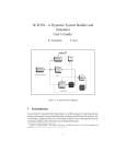
Associated with each signal, in Scicos, is a set of time indices, called activation times, on which the signal can
evolve. Outside their activation times, Scicos signals remain constant (see Figure 1). The activation time set is a union
of time intervals and isolated points called events.
∗ Scicos
is a Scilab toolbox. This version of Scicos is included in Scilab-3.1.1. For more information see: http://www.scicos.org
1
signal remains constant outside
of activation
time
discrete activation
times (events)
continuous
activation time
Figure 1: A signal in Scicos and its activation time set.
Signals in Scicos are generated by blocks driven by activation signals. An activation signal causes the block to
evaluate its output as a function of its input and internal state. It also causes the block to update its states, if any. The
output signal, which inherits its activation time set from the generating block, can be used to drive other blocks.
Blocks are activated by activation signals which are received on activation input ports placed on top of them. A
block with no input activation port is either permanently active (called time dependent) or it inherits its activation times
from the union of activations times of its input signals. If the block is neither permanently active nor has any inputs,
then it is never active during simulation; it is a constant block.
Ports placed at the bottom of blocks are output activation ports. The outgoing signals are activation signals generated by the block. For example, the Clock block generates an activation signal composed of a train of regularly
spaced events in time. If this output is connected to the input activation port of a scope block (such as the MScope
block), it specifies at what times the value of the inputs of the scope must be displayed.
2 Scicos editor
In Scicos, systems are modeled by interconnecting blocks and subsystems (Super blocks); blocks can be found in
various palettes or be defined by user. Scicos has an easy to use graphical user interface for editing diagrams. To start
the editor, in Scilab, type scicos();. This opens up Scicos’ main window.
Construction of Scicos model typically consists of
• opening one or more palettes (using Palettes button in the Edit menu),
• copying blocks from palettes into Scicos’ main window; this can be done by selecting the copy button in the
Edit menu, then clicking on the block to be copied, and finally in the Scicos’ main window, where the block
is to be placed.
• connecting the input and output ports of the blocks by selecting first the link button in the Edit menu, then
clicking on the output port and then on the input port (or intermediary points before that).
Note that to make a link originate from another link (to split a link), user should first click on an existing link, where
split is to be placed, and then on an input port (or intermediary points before that). The process of link creation can be
stopped and current link deleted by clicking on the right mouse button.
Note also that at least one scope or a “write to file” block should be placed in any Scicos diagram to visualize or
save the result of the simulation. See Scicos demos for examples.
2
In addition to pull down menus, Scicos functionalities can also be used through keyboard shortcuts (user definable)
and pop-up menu (click on the right button).
2.1 Parameter adaptation
Block parameters can be modified by opening the block dialogs. This can be done using the Open/set button. Most
blocks have dialog menus which can be used to set or modify block parameters. These parameters can be defined
using valid Scilab expressions. Scilab variables can be used in the definition of these expressions if they are already
defined in the context of the diagram. These expressions are memorized symbolically, and then evaluated.
The context of the diagram can be edited by selecting the Context button. It can contain any valid Scilab
instruction including exec instructions to run Scilab scripts defined on file. Note that in this latter case, if the files are
edited, the user should explicitely use the Eval button to update the block parameters.
2.2 Simulation
A completed diagram can be simulated using Run in the Simulate menu. Selecting this button results in a compilation of the diagram (if not already compiled) and simulation. The simulation can be stopped by clicking on the stop
button on top of the Scicos main window.
A compiled Scicos diagram, saved as a *.cos file, does not need compilation the next time it is loaded; the saved
file contains, the result of the compilation. It is also possible to extract just the data needed to do simulation, and do
the simulation without having to enter the Scicos environment. This can be done using the scicosim function.
2.3 Other functionalities
The editor provides many other functionalities such as
• saving and loading diagrams in various formats
• zooming and changing the point of view
• changing block aspects and colors
• changing diagram’s background and forground colors
• placing text in the diagram
• printing and exporting Scicos diagrams
• and many other standard GUI functions.
The Help button can be used to obtain help on various aspects of Scicos. Selecting Help and then clicking on a block
displays the manual page of the block. Selecting Help and then selecting another button, displays the manual page of
the button.
Finally, an important feature in Scicos is the possibility of creating sub-systems (Super Blocks). Clearly, it would
not be desirable to fit a complex system with hundreds of components in one Scicos diagram. For that, Scicos provides
the possibility of grouping blocks together and defining sub-diagrams called Super Blocks. These blocks behave like
any other block but can contain an unlimited number of blocks, and even other Super Blocks.
3 Basic Blocks
3.1 Explicit Blocks
There are two types of Basic Explicit Blocks in Scicos: Regular Basic Blocks and Synchro Basic Blocks.
3
3.1.1 Regular Basic Block
Regular Basic Blocks (RBB) can have two types of inputs and two types of outputs ports: regular inputs, activation
inputs, regular outputs and activation outputs ports. Regular inputs and outputs are interconnected by regular links,
and activation inputs and outputs, by activation links. Note that activation input ports are placed on top and activation
output ports at the bottom of the blocks.
Such a block can have a continuous state x and a discrete state z. If it does have an x and if u denotes its regular
input, then, when the block is active over an interval of time, x evolves continuously according to
x˙ = f (t, x, z, u, p, ne)
(1)
where f is a vector function, p is a vector of constant parameters and n e is the activation code which is an integer
designating the port(s) through which the block is activated. In particular, if activating input ports are i 1 , i2 , . . . , in ,
then
n
X
ne =
ij 2ij −1 .
j=1
On the other hand, activated by an event, the states x and z jump instantaneously according to the following
equations:
−
x(te ) = gc (te , x(t−
e ), z(te ), u(te ), p, ne )
(2)
−
gd (te , x(t−
e ), z(te ), u(te ), p, ne )
(3)
z(te ) =
where te denotes the event time. The discrete state z remains constant between any two successive events so z(t −
e )
can be interpreted as the previous value of z.
During activation times, the regular output of the block is defined by
y(t) = h(t, x(t− ), z(t− ), u(t), p, ne )
(4)
and is constant when the block is not active.
Finally, RBB’s can generate activation signals of event type. If it is activated by an event at time t e , the time of
each output event is given by
tevo = k(te , z(te ), u(te ), p, ne )
(5)
where tevo is a vector of time, each entry of which corresponds to one activation output port. The absence of event
corresponds to a time smaller than the current time. Event generations can also be pre-scheduled. Pre-scheduling of
events can be done by setting the ”initial firing variables of blocks with event output ports.
There are situations where a block is activated not from an outside activation source but because of an internal
zero-crossing. A zero-crossing occurs when a zero-crossing surface traverses zero. A block can have any number of
zero-crossing functions (surfaces):
s(t) = k(t, x(t), z(t), u(t)).
(6)
When a zero-crossing occurs, the block is internally activated, which is similar to an external activation with n e = −1.
Zero-crossing is used for example to generate zero-crossing events. A few examples of blocks generating output
activations following a zero-crossing can be found in the Threshold palette.
Zero-crossing, in conjunction with the mode flag (not discussed here) is also used to model non-smooth dynamics
of certain blocks. Consider for example the absolute-value block: y = u if u ≥ 0, and y = −u otherwise. This
function is not differentiable at 0. In this case, a mode is defined to specify at the start of the integration period
whether u is positive. To make sure the integration stops when the sign of u changes, a zero-crossing surface is
introduced at zero. During the integration period (which could end because of the zero-crossing), the output y is
computed as follows: y = u if m = 1, and y = −u otherwise. After the zero-crossing the mode is recomputed and
the integration continues.
4
fibo
$
1/u
00000.00
$
Figure 2: An example using Regular Basic Block.
3.1.2 Synchro Basic Block
Beginning from Scilab-2.7 version, custom-made Synchro blocks have been eliminated. There are now only two
Synchro blocks : IF-THEN-ELSE and ESELECT in the Branching palette (see Fig. 4). Synchro Basic Blocks
(SBB) generate output activation signals that are synchronized with their input activation signals. These blocks have
a unique activation input port; they route their input activation signals to one of their activation outputs. The choice of
this output depends on the value of the regular input.
These two important blocks play the role of conditional statements in programming languages such as C.
3.2 Implicit blocks
Differential-algebraic equations (DAE) have the form M (t).y 0 = f (t, y, u) where M is a singular matrix or more
simpler, y is a regular output and u the regular input.
DAE’s of (index 1) can be solved by the implicit solver (DASKR) used in Scicos. DIFF f and CONSTRAINT f
are general Implicit Blocks. However implicit blocks are included in Scicos to allow the integration of Modelica
blocks.
4 Time dependence and inheritance
To avoid explicitly drawing all the activation signals in a Scicos diagram, a feature called inheritance is provided in
Scicos. In particular, if a block has no activation input port, it inherits its activation signal from its regular input signals.
And for blocks which are active permanently, they can be declared as such (“time dependent”) and they do not need
input activation ports. Note that time dependent blocks do not inherit.
5
demo6
+ to −
− to +
xd=Ax+Bu
y=Cx+Du
Figure 3: An example using a block with zero-crossing surface.
5 Block construction
A new block can be constructed as a Super Block (by interconnection of basic blocks) and compiled. As for a new
basic block, it can be defined by a pair of functions:
• an Graphical Interfacing function for handling the user-interface
• a Computational function for specifying its dynamic behavior.
The Graphical Interfacing function is always written as a Scilab function. See Scilab functions in <SCIDIR>/macros/scicos b
for examples. The Computational function can be written in C or Fortran. See <SCIDIR>/routines/scicos
for examples. But it can also be written in Scilab language. C and Fortran routines dynamically linked or permanently
interfaced with Scilab give the better results as far as simulation performance is concerned.
The Scifunc, GENERIC, C block and Fortran block blocks provide generic Graphical Interfacing functions, very useful for rapid prototyping and testing user-developed Computational functions.
5.1 Graphical Interfacing function
The Graphical Interfacing function determines the geometry, color, number of ports and their sizes, icon, etc..., in
addition to the initial states, parameters. This function also handles the block’s user dialog.
What the interfacing function should do and should return depends on an input flag job. The syntax is as follows:
5.1.1 Syntax
[x,y,typ]=block(job,arg1,arg2)
6
Synchro
Abs
event select
If in>0
sinusoid
generator
then
cos
else
S/H
MScope
Figure 4: An example using the two Synchro Basic Blocks.
Parameters
• job==’plot’: the function draws the block.
– arg1 is the data structure of the block.
– arg2 is not used.
– x,y,typ are not used.
In general, we can use standard draw function which draws a rectangular block, and the input and output
ports. It also handles the size, icon, and color aspects of the block.
• job==’getinputs’: the function returns position and type of input ports (regular or activation).
– arg1 is the data structure of the block.
– arg2 is not used.
– x is the vector of x coordinates of input ports.
– y is the vector of y coordinates of input ports.
– typ is the vector of input ports types (1 for regular and 2 for activation).
In general, we can use the standard input function.
• job==’getoutputs’: returns position and type of output ports (regular and activation).
– arg1 is the data structure of the block.
– arg2 is not used.
7
Implicit_Explicit
sinusoid
generator
Qe
Imp_Exp
0.01
220
50
Qe
Qi
Imp2 Qs
S/H
If in>0
then
random
generator
else
MScope
Figure 5: An example using implicit and explicit blocks. The Modelica extension (not discussed here) provides a more
natural setting for this type of modeling.
8
– x is the vector of x coordinates of output ports.
– y is the vector of y coordinates of output ports.
– typ is the vector of output ports types .
In general, we can use the standard output function.
• job==’getorigin’: returns coordinates of the lower left point of the rectangle containing the block’s silhouette.
– arg1 is the data structure of the block.
– arg2 is not used.
– x is the x coordinate of the lower left point of the block.
– y is the y coordinate of the lower left point of the block.
– typ is not used.
In general, we can use the standard origin function.
• job==’set’: opens up a dialogue for block parameter acquisition (if any).
– arg1 is the data structure of the block.
– arg2 is not used.
– x is the new data structure of the block.
– y is not used.
– typ is not used.
• job==’define’: initialization of block’s data structure (name of corresponding Computational function, type,
number and sizes of inputs and outputs, etc...).
– arg1, arg2 are not used.
– x is the data structure of the block.
– y is not used.
– typ is not used.
5.1.2 Block data-structure definition
Each Scicos block is defined by a Scilab data structure as follows:
mlist([’Block’,’graphics’,’model’,’gui’,’doc’],..
graphics,model,gui,doc)
where gui is a string containing the name of the corresponding Graphical Interfacing function and graphics is the
structure containing the graphical data:
graphics= mlist([’graphics’,’orig’,’sz’,’flip’,’exprs’,..
’pin’,’pout’,’pein’,’peout’,’gr_i’,’id’],orig,..
sz,flip,exprs,pin,pout,pein,peout,gr_i,id)
• orig: 2 x 1 vector, the coordinate of down-left point of the block shape.
• sz: vector [w,h], where w is the width and h the height of the block shape.
• flip: boolean, the block orientation. If true the input ports are on the left of the box and output ports are on the
right. if false the input ports are on the right of the box and output ports are on the left.
9
• exprs: column vector of strings, contains expressions answered by the user at block set time.
• pin: column vector of integers. If pin(k)¡¿0 then kth input port is connected to the pin(k)¡¿0 block, else the port
is unconnected. If no input port exist pin==[].
• pout: column vector of integers. If pout(k)¡¿0 then kth output port is connected to the pout(k)¡¿0 block, else the
port is unconnected. If no output port exist pout==[].
• pein: column vector of ones. If pein(k)¡¿0 then kth event input port is connected to the pein(k)¡¿0 block, else
the port is unconnected. If no event input port exist pein==[].
• peout: column vector of integers. If peout(k)¡¿0 then kth event output port is connected to the peout(k)¡¿0
block, else the port is unconnected. If no event output port exist peout==[].
• gr i: column vector of strings, contains Scilab instructions used to customize the block graphical aspect. This
field may be set with ”Icon” sub menu.
• id: string unused.
The data structure containing simulation information is model:
model=mlist([’model’,’sim’,’in’,’out’,’evtin’,’evtout’,..
’state’,’dstate’,’rpar’,’ipar’,’blocktype’,’firing’,..
’dep_ut’,’label’],sim,in,out,evtin,evtout,state,..
dstate,rpar,ipar,blocktype,firing,dep_ut,label)
• sim: list containing two elements. First element is a string containing the name of the Computational function
(fortran, C, or Scilab function). Second element is an integer specifying the type of the Computational function.
The type of a Computational function specifies essentially its calling sequence; more on that later.
• #in: vector of size equal to the number of block’s regular input ports. Each entry specifies the size of the
corresponding input port. A negative integer stands for “to be determined by the compiler”. Specifying the
same negative integer on more than one input or output port tells the compiler that these ports have equal sizes.
• #out: vector of size equal to the number of block’s regular output ports. Each entry specifies the size of the
corresponding output port. Specifying the same negative integer on more than one input or output port tells the
compiler that these ports have equal sizes.
• #evtin: vector of size equal to the number of activation input ports. All entries must be equal to 1. Scicos does
not support vectorized activation links.
• #evtout: vector of size equal to the number of activation output ports. All entries must be equal to 1. Scicos
does not support vectorized activation links.
• state: column vector of initial continuous state.
• dstate: column vector of initial discrete state.
• rpar: column vector of real parameters passed on to the corresponding Computational function.
• ipar: column vector of integer parameters passed on to the corresponding Computational function.
• blocktype: string. Basic block type: ’z’ if ZBB, ’l’ if SBB and anything else for except ’s’ for RBB.
• firing: column vector of initial firing times of size equal to the number of activation output ports of the block. It
includes preprogrammed event firing times (<0 if no firing).
• dep ut: [udep timedep]
10
– udep: boolean. True if system has direct feed-through, i.e., at least one of the outputs depends explicitly
on one of the inputs.
– timedep: boolean. True if block is time dependent.
• label: character string, used as block identifier. This field may be set by the label button in Object menu.
5.2 Computational function
The Computational function evaluates outputs, new states, continuous state derivative and the output events timing
vector depending on the type of the block and the way it is called by the simulator.
5.2.1 Behavior
Simulator calls the Computational function for performing different tasks:
• Initialization The simulator calls the Computational function once at the start for state and output initialization
(inputs are not available then). Other tasks such as file opening, graphical window initialization, etc..., can also
be performed at this point.
• Re-initialization The simulator can call the block a number of times for re-initialization. This is another opportunity to initialize states and outputs (e.g. in cold start case). But at this time, the inputs are available.
• Outputs update The simulator calls for the value of the outputs. Thus the Computational function should
evaluate (4).
• States update One or more events have arrived and the simulator calls the Computational function to update
the states x and z according to (2) and (3).
• State derivative computation The simulator is in a continuous phase; the solver requires x.
˙ This means that
the Computational function must evaluate (1).
• Output events timing The simulator calls the Computational function about the timing of its output events.
The Computational function should evaluate (5).
• Ending The simulator calls the Computational function once at the end (useful for closing files, free allocated
memory, etc...).
The simulator uses a flag to specify which task should be performed (see Table 1).
Flag
0
1
2
3
4
5
6
7
9
Task
State derivative computation
Outputs update
States update
Output events timing
Initialization
Ending
Re-initialization for explicit blocks
Re-initialization for implicit blocks
zero-crossing functions and mode
Table 1: Tasks of Computational function and their corresponding flags
11
5.2.2 Types of Computational functions
In Scicos, for to guarantee backward compatibility, Computational functions can be of different types and co-exist in
the same diagram. Old types are listed in Table 2. It is highly recommended to use new types: 4 and 10004 (for C
code), and 5 and 10005 (for Scilab code), from now on.
Function type
0
1
2
3
10001
10002
10003
Scilab
yes
no
no
yes
no
no
yes
Fortran
yes
yes
no
no
yes
no
no
C
yes
yes
yes
no
yes
yes
no
Comments
Fixed calling sequence for explicit blocks
Varying calling sequence for explicit blocks
Fixed calling sequence for explicit blocks
Inputs/outputs are Scilab lists for explicit blocks
Varying calling sequence for implicit blocks
Fixed calling sequence for implicit blocks
Inputs/outputs are Scilab lists for implicit blocks
Table 2: Different types of the Computational functions. Type 0 is obsolete.
Computational function: type 4 All explicit new C blocks should be of type 4. Type 4 blocks should be defined as
follows:
#include "scicos_block.h"
#include <math.h>
void my_block(scicos_block *block,int flag)
{
...
}
The flag is any integer from 0 to 9 indicating the task to be preformed and block is the block structure defined as follows:
typedef struct {
int nevprt;
/*
voidg funpt;
/*
int type;
/*
int scsptr;
/*
int nz;
/*
double *z;
/*
int nx;
/*
double *x;
/*
double *xd;
/*
double *res;
/*
int nin;
/*
int *insz;
/*
double **inptr; /*
int nout;
/*
int *outsz;
/*
double **outptr;/*
int nevout;
/*
double *evout; /*
int nrpar;
/*
double *rpar;
/*
int nipar;
/*
int *ipar;
/*
int ng;
/*
double *g;
/*
binary coding of activation inputs, -1 if internally activated */
pointer: pointer to the computational function */
type of interfacing function, current type is 4 */
not used for C interfacing functions */
size of the discrete-time state */
vector of size nz: discrete-time state */
size of the continuous-time state */
vector of size nx: continuous-time state */
vector of size nx: derivative of continuous-time state */
only used for internally implicit blocks. vector of size nx */
number of inputs */
input sizes */
table of pointers to inputs */
number of outputs */
output sizes */
table of pointers to outputs */
number of activation output ports */
delay times of output activations */
number of real parameters */
real parameters of size nrpar */
number of integer parameters */
integer parameters of size nipar */
number of zero-crossing surfaces */
zero-crossing surfaces */
12
int ztyp;
int *jroot;
char *label;
void **work;
int nmode;
int *mode;
} scicos_block;
/*
/*
/*
/*
/*
/*
boolean, true only if block MAY have zero-crossings */
vector of size ng indicating the presence and direction of crossings */
block label */
pointer to workspace if allocation done by block */
number of modes */
mode vector of size nmode */
The following C functions can be used within a compuational function of type 4 to obtain additional information
and perform other operations:
• double get scicos time(): returns the current time t.
• void set block error(int): used by the block to signal an error to the simulator.
• int get phase simulation(): returns the simulation phase (1 or 2).
• int get block number(): returns the block number.
Computational function: type 5 This type is for computational function expressed in Scilab. The calling sequence
is:
block=func_name(block,flag)
where block is a Scilab structure similar to the C structure used in the C computational function of type 4. The fields
of block are
scicos_block nevprt funpt type scsptr nz z nx x xd
nin insz inptr nout outsz outptr nevout evout nrpar
nipar ipar ng g ztyp jroot label work nmode mode
res
rpar
The following Scilab functions can be used to obtain additional information and perform other operations:
• curblock(): returns the current block number in the structure %cpr.
• scicos time(): gives the current time.
• phase simulation(): returns the simulation phase.
• set blockerror(i): set the error flag if the computational function encounters an error.
Examples Consider the following computational function, which is the code for the summation block in Scicos; it
is of type 4.
#include "scicos_block.h"
#include <math.h>
void summation(scicos_block *block,int flag)
{
int j,k;
if(flag==1){
if (block->nin==1){
block->outptr[0][0]=0.0;
for (j=0;j<block->insz[0];j++) {
block->outptr[0][0]=block->outptr[0][0]+block->inptr[0][j];
}
}
else {
13
for (j=0;j<block->insz[0];j++) {
block->outptr[0][j]=0.0;
for (k=0;k<block->nin;k++) {
if(block->ipar[k]>0){
block->outptr[0][j]=block->outptr[0][j]+block->inptr[k][j];
}else{
block->outptr[0][j]=block->outptr[0][j]-block->inptr[k][j];
}
}
}
}
}
}
The following is a simple example of the compuational function of a type 5 block. This block realizes the sine
function.
function block=sin5(block,flag)
if flag==1 then
for j=1:block.insz(1)
block.outptr(1)(j)=sin(block.inptr(1)(j));
end
end
endfunction
Computational functions: type 10004 and 10005 These types are used to construct implicit blocks. They are not
discussed here. Type 10004 is used mostly by the Modelica extension.
6 Conclusion
This document gives only a brief description of Scicos and its usage. More information can be found in the manual
pages of Scicos functions (Scilab help under Scicos library). Scicos demos provided with Scilab constitute also an
interesting source of information. Often, it is advantageous to start off from and edit a Scicos demo rather than starting
with an empty diagram.
More information is available on www.scicos.org.
14