Download User Manual - The Virtual Physiological Rat Project

BISEN: Biochemical Simulation Environment
User’s Manual
Version 1.0.6
http://bbc.mcw.edu/BISEN
c
2008
Medical College of Wisconsin, Inc. All rights reserved.
1
Contents
1 Introduction
1.1 MATLAB Programming Environment . . . . . . . . . . . . . . . . . . . . . . . . . . . . . .
1.2 Setting Paths . . . . . . . . . . . . . . . . . . . . . . . . . . . . . . . . . . . . . . . . . . . .
3
3
3
2 Overview of Package and Description of Files
2.1 Biochemical Thermodynamic Data and Reaction and Transporter Stoichiometry . . . . . .
2.2 Model Component Modules for Enzymes and Transporters . . . . . . . . . . . . . . . . . . .
2.3 MATLAB Scripts for Generating Models . . . . . . . . . . . . . . . . . . . . . . . . . . . . .
5
5
7
9
3 Creating Biochemical Systems Models
11
3.1 Example 1: ATP Hydrolysis . . . . . . . . . . . . . . . . . . . . . . . . . . . . . . . . . . . . 12
4 More Examples
19
4.1 Example 2: A Two-Compartment System with a Membrane Potential . . . . . . . . . . . . 19
4.2 Example 3: Computer Model of Mitochondrial TCA Cycle and Oxidative Phosphorylation . 22
4.2.1 Interacting with large scale models . . . . . . . . . . . . . . . . . . . . . . . . . . . . 25
4.2.2 Simulating the experiments . . . . . . . . . . . . . . . . . . . . . . . . . . . . . . . . 26
4.3 Conserved pools . . . . . . . . . . . . . . . . . . . . . . . . . . . . . . . . . . . . . . . . . . 27
5 Further Information
5.1 Where to Get BISEN . . . .
5.2 Bug Reporting and Tracking
5.3 Future Plans . . . . . . . . .
5.3.1 Additional ion binding
5.3.2 Model reduction . . .
.
.
.
.
.
.
.
.
.
.
.
.
.
.
.
.
.
.
.
.
.
.
.
.
.
.
.
.
.
.
.
.
.
.
.
.
.
.
.
.
.
.
.
.
.
.
.
.
.
.
.
.
.
.
.
.
.
.
.
.
.
.
.
.
.
.
.
.
.
.
.
.
.
.
.
.
.
.
.
.
.
.
.
.
.
.
.
.
.
.
.
.
.
.
.
.
.
.
.
.
.
.
.
.
.
.
.
.
.
.
.
.
.
.
.
.
.
.
.
.
.
.
.
.
.
.
.
.
.
.
.
.
.
.
.
.
.
.
.
.
32
32
32
32
32
32
6 Thermodynamics of biochemical reactions
6.1 Definitions . . . . . . . . . . . . . . . . . . .
6.2 NPT Ensemble . . . . . . . . . . . . . . . .
6.3 Electrophysiology . . . . . . . . . . . . . . .
6.4 Proton and ion binding . . . . . . . . . . .
6.5 Temperature and ionic strength dependence
6.6 Carbon dioxide . . . . . . . . . . . . . . . .
.
.
.
.
.
.
.
.
.
.
.
.
.
.
.
.
.
.
.
.
.
.
.
.
.
.
.
.
.
.
.
.
.
.
.
.
.
.
.
.
.
.
.
.
.
.
.
.
.
.
.
.
.
.
.
.
.
.
.
.
.
.
.
.
.
.
.
.
.
.
.
.
.
.
.
.
.
.
.
.
.
.
.
.
.
.
.
.
.
.
.
.
.
.
.
.
.
.
.
.
.
.
.
.
.
.
.
.
.
.
.
.
.
.
.
.
.
.
.
.
.
.
.
.
.
.
.
.
.
.
.
.
.
.
.
.
.
.
.
.
.
.
.
.
.
.
.
.
.
.
.
.
.
.
.
.
.
.
.
.
.
.
33
33
33
35
35
38
39
.
.
.
.
.
.
.
.
.
.
.
.
.
.
.
.
.
.
.
.
.
.
.
.
.
.
.
.
.
.
.
.
.
.
.
2
Chapter 1
Introduction
The Biochemical Simulation Environment (BISEN) software package is a suite of tools for generating equations and associated computer programs for simulating biochemical systems. The Version 1.0 package can
be used to generate appropriate systems of differential equations for user-specified multicompartment systems of enzymes and transporters accounting for detailed biochemical thermodynamics, rapid equilibria of
multiple biochemical species, and dynamic proton and metal ion buffering. The basic theory and methodology associated with this tool is outlined briefly in chapter 6, but described in some detail in Vinnakota et
al. [7]. Biochemical system components are specified using a human read/writeable biochemical scripting
language; model outputs are in the form of a MATLAB M-file that computes the differential equations for
the systems.
The package was constructed and is maintained and distributed by the computational biology group in
the Biotechnology and Bioengineering Center at the Medical College of Wisconsin. The package, updates,
and other information can be obtained at the URL http://bbc.mcw.edu/Bisen. When reporting on work
that makes use of this package, please cite the following reference:
Vanlier J, Wu F, Qi F, Vinnakota KC, Han Y, Dash RK, Yang F and Beard DA. BISEN: Biochemical
Simulation Environment. Bioinformatics 25(6):836-837, 2009.
The following sections of this manual provide step-by-step instructions on how to use the package
based on tutorial examples at different levels of complexity, and further information on how the package
is maintained and updated.
1.1
MATLAB Programming Environment
The current version of the BISEN Package utilizes the propriety MATLAB (Mathworks Inc.) programming
environment. Running the package requires that the user have MATLAB installed with a current license.
The BISEN package has been tested on MATLAB Release R2008a.
1.2
Setting Paths
All of the files associated with the package must be in the MATLAB path or in the current working directory in order for the model building engine to work. In the archive in which the package is distributed, the
package is organized to include seven subdirectories ‘Transporters’ and ‘BiochemicalReactions’, in which
model modules are stored, ‘Warnings’, in which error warnings are stored, ‘Databases’, in which reaction,
3
transport and reactant databases are stored, ‘BuilderFiles’, in which builder files are stored, ‘ExperimentalData’, in which experimental data required by computational simulation are stored,‘Examples’, in which
all the examples are stored. If this file structure is maintained and all files and directories exist in the
current working directory, then paths can be set in MATLAB with the following commands.
For Windows-Based Systems:
path(path,’..\Warnings’);
path(path,’..\BiochemicalReactions’);
path(path,’..\Transporters’);
path(path,’..\Databases’);
path(path,’..\BuilderFiles’);
path(path,’..\ExperimentalData’);
path(path,’..\Examples’);
For Linux-Based Systems:
path(path,’.\Warnings’);
path(path,’.\BiochemicalReactions’);
path(path,’.\Transporters’);
path(path,’.\Databases’);
path(path,’.\BuilderFiles’);
path(path,’.\ExperimentalData’);
path(path,’.\Examples’);
4
Chapter 2
Overview of Package and Description of
Files
The BISEN package uses a text parsing algorithm to translate a simple list of biochemical system components into a set of differential equations in a MATLAB M-file. This section provides a reference list of file
types used and constructed by the BISEN package. User-constructed input files make use of a Biochemical Scripting Language (BSL), described below in Section 3 along with detailed instructions on how to
construct models using the package.
2.1
Biochemical Thermodynamic Data and Reaction and Transporter
Stoichiometry
Physicochemical data on biochemical reactants and reactions are stored in the three Excel spreadsheet
files listed below. These files provide data on more than 50 reactions and transport processes and over
100 associated biochemical reactants along with their respective references denoted in the cell comments.
The reactants and reactions included in these databases define the scope of possible models that can be
constructed with the package. Users may add additional reactants and reactions to these databases in
order to be able to expand the package’s capabilities for their specific applications. When doing so, users
are urged to proceed with appropriate care and caution.
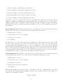
ReactantDatabase.xls. This file specifies the basic thermodynamic and ion binding data for biochemical
reactants. For each reactant entry the following information is provided:
1. Detailed name of reactant.
2. Abbreviation used for model description.
3. Gibbs free energy of formation for reference species associated with reactant.
4. Enthalpy of formation for reference species.
5. Charge of references species.
6. Number of protons in reference species.
7. First proton dissociation constant, given as pK, the negative of the base-10 logarithm of the dissociation constant.
5
8. Reaction enthalpy of the first proton dissociation
9. First potassium ion dissociation constant, given as pK.
10. Reaction enthalpy of the first potassium dissociation
11. First magnesium ion dissociation constant, given as pK.
12. Reaction enthalpy of the first magnesium dissociation
The symbol ‘#’ is used to indicate lack of data for a particular entry. When not specified, the pK’s are
assumed to be infinite (no binding) with corresponding dissociation constants equal to zero. Gibbs energies,
enthalpies and dissociation constants are tabulated at 298.15 K, while reactants are tabulated at 0 M ionic
strength and dissociation constants at 0.1 M ionic strength. The sources of the constants are given in the
cell comments.
ReactionDatabase.xls. This file specifies the reference stoichiometry associated with chemical reactions
available in the database. For each reaction, the following information is provided:
1. Detailed name of reaction.
2. Abbreviation used for model description.
3. Stoichiometry of reaction.
4. E. C. Number.
It is important to note three important features regarding the reaction stoichiometries provided in this
file: (1.) the specification is for reference reactions, in terms of the reference species defined in the
reactant database (ReactantDatabase.xls); (2.) protons (designated by ‘H’ in the reaction equations)
appear explicitly as chemical species in reference reactions; (3.) the reactions use the abbreviations defined
in the reactant database (ReactantDatabase.xls). Mismatches between abbreviations used here and those
used in the reactant database will lead to errors; (4.) when specifying the reference reaction one should be
careful that all the operators, coefficients and reactants are separated by spaces.
TransportDatabase.xls. This file specifies the reference stoichiometry associated with chemical transporters available in the database. For each reaction, the following information is provided:
1. Detailed name of reaction.
2. Abbreviation used for model description.
3. Stoichiometry of reaction.
4. Charge translocated by the transporter.
5. E. C. Number.
Each reference transport reaction involves two compartments. The two compartments are specified in
the stoichiometric equation using the identifiers ‘(1)’ and ‘(2)’ following each species abbreviation. For
example, the stoichiometric equation
ATP(1) = ATP(2)
6
indicates that ATP is transported from the first to the second compartment. The charge entry indicates
how many charges are transported from compartment 2 to compartment 1. Therefore, for example, the
stoichiometric equation
ATP(2) + ADP(1) = ATP(1) + ADP(2)
has associated with it a charge translocation value of −1, meaning that one charge is translocated from
compartment 1 to 2 every time this transport reaction turns over. This reaction actually involves exchanging an ATP (with charge −4) for an ADP (with charge −3), for an overall transfer of −1 from compartment
2 to 1. Please note that when a transport process occurs at a porous membrane, which is highly permeable
to small-size ions, the charge entry for that transport process is adjusted to 0.
When a transporter transports a reactant that is bound to an ion use square brackets to include the ion
transport. An example of this is the proton transported along with glutamate in the glutamate/aspartate
anti-transporter.
[H](2) + glutamate(2) + aspartate(1) = [H](1) + aspartate(2) + glutamate(1)
2.2
Model Component Modules for Enzymes and Transporters
The directories ‘BiochemicalReactions’ and ‘Transporters’ contain files that provide computational models
to simulate the kinetics of individual enzymes and transporters. The format and specifications of these
files are described below.
Biochemical Reactions
This directory contains a file for each reaction specified in the reaction database ReactantDatabase.xls.
The file names are the reaction abbreviations with the file extension ‘.txt’. For example, the kinetic model
module for the creatine kinase reaction is provided in the text file ‘CK.txt’.
Each of these reaction files list the equations required to simulate the kinetics of the enzyme. To account for multiple model versions and allow for nonreacting allosteric species to influence reaction kinetics,
the model syntax makes use of a number of keywords. These keywords are listed below:
Keyword
model
allosteric reactants
equations
EOF
Meaning
This keyword indicates the beginning of a new model version for a particular enzyme or transporter. The keyword ‘model’ is followed by an identifier
associated with the model. A few lines of text can optionally be specified to
describe the model, as long as they do not contain any keywords.
Reactants that do not appear in the biochemical reaction but may influence the
reaction’s kinetics must be listed as allosteric reactants following this keyword.
The model equations, using matlab syntax are listed following this keyword.
Indicates the end of the file
7
In addition the protected variable names used in the model equations are listed below:
Protected Variable
J
Keq
unspecified
Ky x
Px
h, m, k
V
Reactant Abbreviations
Meaning
This variable is use to specify the flux through the reaction. Each submodel
must specify the resulting flux.
This variable references the apparent equilibrium constant for the reaction or
transporter.
This keyword, when appearing in the model equations, indicates the introduction of an unspecified model parameter.
This variable indicates the dissociation constant of species X with ion Y. For
example Kh ATP will refer to the proton dissociation constant of ATP.
This variable indicates the binding polynomial of reactant x. The binding
polynomial can be used to compute a specific species concentration.
These variables reference the proton, magnesium and potassium concentration.
The volume of this compartment
Each reactant concentration is referenced by its abbreviation.
To illustrate how these keywords and protected variable names are applied, consider the following
examples.
The file ‘CK.txt’ contains the following text:
model E.CK.0
equations
k1_CK = unspecified;
J = k1_CK*(phosphocreatine*ADP - creatine*ATP/Keq);
model E.CK.1
equations
x_CK = 1e7;
CRtot = 42.7e-3;
K_CK = exp(50.78/RT);
Cr_c
= CRtot - phosphocreatine;
ATP_c1 = ATP * 1/P_ATP; % Mg2+ unbound species;
ADP_c1 = ADP * 1/P_ADP; % Mg2+ unbound species;
J = x_CK * (K_CK*ADP_c1*phosphocreatine*h - ATP_c1*Cr_c );
EOF
In this case, there are two possible models of this enzyme, E.CK.0 and E.CK.1, that may be invoked when
building a model including creatine kinase. The first one is a simple mass action model, while the second
model invokes more complex reaction kinetics.
In model E.CK.0 the apparent rate constant for the reaction ‘k1 CK’ is a parameter with an unspecified
value. Model E.CK.1 invokes no unspecified parameters.
8
The E.CK.0 model invokes the protected variable name Keq, which the model-builder will recognize
as the apparent equilibrium constant for the CK reaction. That means that the variable Keq in the
flux expression will be replaced with the apparent equilibrium constant, computed as a function of ionic
strength, temperature, pH, and metal ion concentrations in the kinetic model. The second model uses
a user-specified equilibrium constant variable K CK, which is set to a constant value, and therefore not
computed using the built-in thermodynamic database or adjusted for the possibly variable biochemical
state of the model.
The dissociation constants and binding polynomials can be used to compute specific species. For
example, the magnesium bound ATP concentration can be calculated as follows:
MgATP = (ATP/P_ATP)*(m/10^(-Km_ATP))).
Transporters
The transporter files are similar in terms of structure and keywords. However, in the case of a transporter,
each state variable name is followed by a compartment number. In these equations, the compartment
number is defined so that (1) refers to the from compartment and (2) refers to the destination compartment.
An example of this is a model for the permeation of glutamate.
model T.GLUPERM.0
equations
x_GLUPERM = unspecified;
J = gamma * x_GLUPERM * (glutamate(1) - glutamate(2));
EOF
2.3
MATLAB Scripts for Generating Models
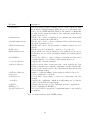
The M-files included with the BISEN model-building package are listed in Table 2.1. The file names in
italics are files required by the builder. These files are organized in sub-folders in the package distribution
and should be in the current path wherever the user chooses to work.
9
File Name
BuildDXDT.m
setParameter.m
generateParameterset.m
validateParameters.m
checkPools.m
validateParameters.m
IndexPHMK.m
conservationMatrix.m
readReactionEntry.m
readTransportEntry.m
str2array.m
IonTempCorr.m
convertKi.m
getISCF.m
BISENlogo.m
appendCompName.m
Description
This is the main program for parsing a model described in the modular
Biochemical Scripting Language (BSL) into a set of differential equations coded in a MATLAB M-file function. The syntax for running this
program and the syntax and features of the input and output files are
described in Section 3.
This file can be used for adjusting model constants and setting initial
conditions by name rather than index.
This file can be used to generate a human-readable m-file that returns
the supplied parameter vector.
This file can be used to check a parameter or initial condition vector for
validity.
This file is used for checking the conserved pools of a model.
Checks whether the current parameter set is sufficient for the model.
It will throw an error when something is missing and identify what is
missing.
Used by the builder to replace binding polynomials and dissociation
constants with the correct variables when parsing submodels.
Computes the conservation matrix
Reads a reaction submodel and parses the content replacing the equilibrium constant keyword with the equilibrium constant variable name
specific for the current reaction. Also substitutes the flux and δΨ variables in a similar manner.
Similar to readReactionEntry, parses transporter submodel however.
Convert a string into a cell array.
Corrects Gibbs energy change of reaction for temperature and ionic
strength.
Computes the equilibrium constant from pKa taking into account the
desired ionic strength and temperature.
Computes the factors needed for IonTempCorr.m and computeKi.m
Used for displaying the BISEN logo
Used by the builder to append the compartment names to state variables
in equations.
Table 2.1: M-files included in the BISEN package
10
Chapter 3
Creating Biochemical Systems Models
Systems models are specified using the Biochemical Scripting Language (BSL), which facilitates simple
flexible and modular specification of complex models.
A BSL file lists the compartments that make up a model, along with the enzymes present in each
compartment and transporters that transport mass between compartments. BSL files use several keywords
that demarcate different input sections of the file:
11
Keyword
ionic strength
temperature
globals
export
compartment
transport
clamped
permeate
EOF
3.1
Meaning
This keyword is followed by a value which specifies the ionic strength of the
solution. If omitted an ionic strength of 0.17 M (estimated from a muscle cell)
is assumed. Note that this optional keyword has to be specified at the start
of the bsl file.
This keyword is followed by a value which specifies the experimental temperature in Celsius. If omitted a temperature of 37.0o C (i.e. 298.15o K) is assumed.
Note that this optional keyword has to be specified at the start of the bsl file.
The first lines after the optional ionic strength and/or temperature setting
can be used for parameters that can be accessed by all submodels. Regular
matlab code is acceptable in this first section. Here the keyword unspecified,
specifies that value will become a model parameter (e.g. Ca = unspecified;).
The keyword export can be used at the end of the section where globals are
specified to export any internal variables. The model will only export the
value that was assigned to the variable last.
Entries following this keyword define a compartment name and volume followed by a list of the enzymes to be included in the specified compartment.
Entries following this keyword define two linked compartments and list the
transporters to be included in the model. Note that all compartments have to
be defined before defining transporters.
After specifying the list of reactions or transporters, in a compartment or
transport block certain concentrations can be specified as clamped using this
keyword. Clamping a variable means manually setting the time derivative to
zero. In the case of a transport field, this will clamp the state variable in
both compartments. If the parser is unable to find the value that needs to be
clamped it will throw a warning, but continue parsing nontheless.
This keyword is used to specify species or ions that passively permeate across
compartment barriers. These species are not affected by the compartimentalization.
This keyword indicates the end of a file.
Example 1: ATP Hydrolysis
As a fist simple example, consider building a one-compartment model including the ATP hydrolysis reaction. A model of this system is specified in the BSL model file ‘Example1.bsl’, which is distributed with
the BISEN Package. This file contains the following entries:
compartment A 1.0 1.0
ATPASE E.ATPASE.0
EOF
Since no commands appear between the start of the file and ‘compartment’, no global model variables are
declared. The ‘compartment’ command declares a compartment, labeled ‘A’, with water content 1.0 and
fractional region volume 1.0. Following the compartment declaration, one reaction (ATPase) is listed, with
the kinetic model E.ATPASE.0 specified.
The ATPASE reaction is found in the Reaction Database, and the model E.ATPASE.0 is specified in
the biochemical reaction module ATPASE.txt. The model generating engine is called to parse this BSL
12
model into a MATLAB ordinary differential equation script using the following syntax.
modelInfo = BuildDXDT(’Example1.bsl’,’dXdT.m’);
The program BuildDXDT.m is passed two input strings, specifying the input BSL file and the name of the
output M-file that is to be built. In this case, the automatically constructed output M-file dXdT.m has
the following contents.
%
%
%
%
%
%
%
%
%
%
%
%
%
%
%
%
%
%
%
%
%
%
%
%
function [f,J,] = dXdT(t,x,T,BX,K_BX,par)
Output parameters:
f
time derivatives of the model
J
flux
Mandatory input parameters:
t
time
x
state variables at t=0
T
temperature in degreesCelcius
BX
buffer sizes
K_BX proton buffer dissociation constants ( A )
par
parameter vector for the free parameters
State Variables:
[ATP_A , ADP_A , Pi_A ]
Free Parameters:
[k1_ATPASE ]
function [f,J,varargout] = dXdT(t,x,T,BX,K_BX,par)
%% GLOBAL VARIABLES
%% LIST OF STATE VARIABLES
% 1 ATP_A
% 2 ADP_A
% 3 Pi_A
% 4 h_A
% 5 m_A
% 6 k_A
% PARTIAL VOLUME FRACTIONS
VWater_A = 1; % [=] l water (l region)^{-1}, Vinnakota and Bassingthwaighte, AJP, 2004
VRegion_A = 1; % [=] l region (l tissue)^{-1}, Vinnakota and Bassingthwaighte, AJP, 2004
13
%% THERMODYNAMIC DATA
RT = 8.314*(T+273.15)/1e3; % kJ mol^{-1}
F = 0.096484; % kJ mol^{-1} mV^{-1}
%% STATE VARIABLES
% Concentrations of Reference Species
ATP_A = x(1);
ADP_A = x(2);
Pi_A = x(3);
% Concentrations of H, Mg, and K
h_A = x(4);
m_A = x(5);
k_A = x(6);
% Membrane potentials
%% DISSOCIATION CONSTANTS
% ATP_A
Kh(1) = 2.7990983755242071e-007;
Km(1) = 0.00010815244062499601;
Kk(1) = 0.097055055483606045;
% ADP_A
Kh(2) = 4.1856568564882887e-007;
Km(2) = 0.00088211913575503352;
Kk(2) = 0.13114858875318428;
% Pi_A
Kh(3) = 2.1306351186738022e-007;
Km(3) = 0.032137949367841569;
Kk(3) = 0.37888645618434613;
%%
P(
P(
P(
BINDING POLYNOMIALS
1 ) = 1 + h_A/Kh(1) + m_A/Km(1) + k_A/Kk(1);
2 ) = 1 + h_A/Kh(2) + m_A/Km(2) + k_A/Kk(2);
3 ) = 1 + h_A/Kh(3) + m_A/Km(3) + k_A/Kk(3);
%% THERMODYNAMIC EQUATIONS
DGro_ATPASE =4.5083;
Keq_ATPASE_A = exp(-DGro_ATPASE/RT)/P(1)*P(2)*P(3)/h_A;
%% FLUX EQUATIONS
%ATPASE_A
k1_ATPASE=par(1);
J_ATPASE_A=k1_ATPASE*(ATP_A-ADP_A*Pi_A/Keq_ATPASE_A);
%% REACTANT TIME DERIVATIVES
14
f(1,:) = ( 0
f(2,:) = ( 0
f(3,:) = ( 0
- 1*J_ATPASE_A ) / VWater_A; % ATP_A
+ 1*J_ATPASE_A ) / VWater_A; % ADP_A
+ 1*J_ATPASE_A ) / VWater_A; % Pi_A
%% ION EQUATIONS
% COMPARTMENT A:
ii = [1 2 3]; % Indices of SVs in compartment A
% PARTIAL DERIVATIVES
pHBpM = -sum( (h_A*x(ii)’./Kh(ii))./(Km(ii).*P(ii).^2) );
pHBpK = -sum( (h_A*x(ii)’./Kh(ii))./(Kk(ii).*P(ii).^2) );
pHBpH = +sum( (1+m_A./Km(ii)+k_A./Kk(ii)).*x(ii)’./(Kh(ii).*P(ii).^2) );
pMBpH = -sum( (m_A*x(ii)’./Km(ii))./(Kh(ii).*P(ii).^2) );
pMBpK = -sum( (m_A*x(ii)’./Km(ii))./(Kk(ii).*P(ii).^2) );
pMBpM = +sum( (1+h_A./Kh(ii)+k_A./Kk(ii)).*x(ii)’./(Km(ii).*P(ii).^2) );
pKBpH = -sum( (k_A*x(ii)’./Kk(ii))./(Kh(ii).*P(ii).^2) );
pKBpM = -sum( (k_A*x(ii)’./Kk(ii))./(Km(ii).*P(ii).^2) );
pKBpK = +sum( (1+h_A./Kh(ii)+m_A./Km(ii)).*x(ii)’./(Kk(ii).*P(ii).^2) );
% PHIs
J_H = (0 + 1*J_ATPASE_A) / VWater_A;
J_M = (0) / VWater_A;
J_K = (0) / VWater_A;
Phi_H = J_H - sum( h_A*f(ii)’./(Kh(ii).*P(ii)) );
Phi_M = -sum( m_A*f(ii)’./(Km(ii).*P(ii)) );
Phi_K = J_K -sum( k_A*f(ii)’./(Kk(ii).*P(ii)) );
% ALPHAs
aH = 1 + pHBpH;
aM = 1 + pMBpM;
aK = 1 + pKBpK;
% ADDITIONAL BUFFER for [H+]
aH = 1 + pHBpH + BX(1)/K_BX(1)/(1+h_A/K_BX(1))^2; % M
% DENOMINATOR
D = aH*pKBpM*pMBpK + aK*pHBpM*pMBpH + aM*pHBpK*pKBpH - ...
aM*aK*aH - pHBpK*pKBpM*pMBpH - pHBpM*pMBpK*pKBpH;
% DERIVATIVES for H,Mg,K
f(4,:) = ( (pKBpM*pMBpK - aM*aK)*Phi_H + ...
(aK*pHBpM - pHBpK*pKBpM)*Phi_M + ...
(aM*pHBpK - pHBpM*pMBpK)*Phi_K ) / D;
f(5,:) = ( (aK*pMBpH - pKBpH*pMBpK)*Phi_H + ...
(pKBpH*pHBpK - aH*aK)*Phi_M + ...
(aH*pMBpK - pHBpK*pMBpH)*Phi_K ) / D;
f(6,:) = ( (aM*pKBpH - pKBpM*pMBpH)*Phi_H + ...
(aH*pKBpM - pKBpH*pHBpM)*Phi_M + ...
(pMBpH*pHBpM - aH*aM)*Phi_K ) / D;
%% ELECTROPHYS EQUATIONS
%% FLUX VECTOR:
J = [ J_ATPASE_A];
15
This file describes a complete model to simulate ATP hydrolysis in a well-mixed aqueous solution. The
function accepts several input variables and outputs the time derivatives of the state variables and the
flux for the chemical reaction, as detailed in the function header. For this example BISEN model builder
creates a model with six state variables: the three reactant concentrations, ATP, ADP, and Pi, and the
three ion concentrations, [H+ ], [Mg2+ ], and [K+ ]. These state variables and there indices are listed in the
comments generated for the model file. (See ‘LIST OF STATE VARIABLES’.)
Using one of the built-in ordinary differential equation solvers in MATLAB, it is fairly straightforward
to simulate this model. The steps are: (1.) Set buffering constant and biochemical state parameters; (2.)
Specify initial values for the state variables; (3.) Run the simulation; and (4.) Plot the results. For this
model, to generate the simulations results illustrated in [6], the following commands are used.
%% Setting up and running Example 1
% (1.) Setting parameter values (no buffering)
B_X
= 0;
% Additional proton buffering capacity
K_BX = 1e-7;
% Dissociation constant of additional proton buffer
par(1) = 0.1;
% k (kinetic constant for ATP hydrolysis)
T = 25;
% Temperature
% (2.) Setting initial values
xo(1) = 10e-3; % [ATP] (M)
xo(2) = 0;
% [ADP] (M)
xo(3) = 0;
% [Pi] (M)
xo(4) = 1e-7;
% [H] (M)
xo(5) = 1e-3;
% [Mg] (M)
xo(6) = 150e-3; % [K] (M)
% (3.) Running for 15-second time course
[t,x] = ode45(@dXdT,[0 15],xo,[],T,B_X,K_BX,par);
% (4.) Plotting results
figure(1); p = plot(t,x(:,1)*1e3,’k-’,t,x(:,2)*1e3,’k-’,t,x(:,5)*1e3,’k-’);
set(p,’linewidth’,1.5);
text(2,9,’[ATP]’,’Fontsize’,14);
text(2,3.5,’[ADP]’,’Fontsize’,14);
text(5,2.3,’[Mg^{2+}]’,’Fontsize’,14);
ylabel(’Concentration (mM)’,’Fontsize’,14);
xlabel(’Time (sec)’,’Fontsize’,14);
set(gca,’Fontsize’,14);
figure(2); plot(t,-log10(x(:,4)),’k-’,’linewidth’,1.5);
ylabel(’pH’,’Fontsize’,14);
xlabel(’Time (sec)’,’Fontsize’,14);
set(gca,’Fontsize’,14);
Note that this script uses the built-in MATLAB ODE integrator function ode45, which is reasonable suited
to this application. Other integrator functions are available in MATLAB and from third-party sources.
More information can be found, for example, by typing doc ode45 at the MATLAB command prompt.
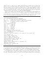
For debugging purposes, a file with the extension .log is also generated, which describes the computation of the Gibbs energies of reaction and the applied temperature and ionic strength corrections. Here,
the values of the indicated variables are denoted between the square brackets and the stoichiometry is
16
shown between parentheses. This can be helpful when problems arise when new data is added to the reactant database. The initial lines show the untransformed Gibbs energies of formation and the associated
stoichiometries of the reactions. These are followed by the ionic strength correction on both the enthalpy
change of the reaction and the Gibbs energy change of the reaction. Finally temperature correction is done
using the transformed enthalpy.
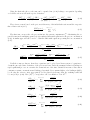
---------------GIBBS ENERGIES
---------------Reaction: ATPASE
0 + (-1)dG_ATP[-2768.100] + (-1)dG_H2O[-237.190] + (1)dG_ADP[-1906.130] +
(1)dG_Pi[-1096.100] + (1)dG_H[0.000]
0 + (-1)dH_ATP[-3619.210] + (-1)dH_H2O[-285.830] + (1)dH_ADP[-2626.540] +
(1)dH_Pi[-1299.000] + (1)dH_H[0.000]
Ionic strength correction: DrG[3.060000] - beta_G[0.724132] * Q[-2.000000]
= 4.508263
Ionic strength correction: DrH[-21.973592] - beta_H[0.368398] * Q[-2.000000]
= -21.236796
Temp correction: drG = (1-Tn[298.15]/To[298.15]) * drH[-21.2368]
+ (Tn[298.15]/To[298.15]) * drG = 4.508263
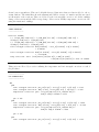
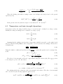
This section is followed by a section outlining the temperature and ionic strength corrections on each of
the pK values.
----------------PKA CORRECTIONS
----------------ATP
pKH
Ionic strength correction: pKa_in[6.710] + beta_K[-0.020] * z[8.000] = 6.553
Ionic strength correction: dHr[-2.000] + beta_H2[0.057] * z[8.000] = -1.544
Temperature correction: pKa + (1/T_new[298.150]-1/T_old[298.150]) *
drH[-1.544]/2.3026*R = 6.553
pK = 0.000
pKM
Ionic strength correction: pKa_in[4.280] + beta_K[-0.020] * z[16.000] = 3.966
Ionic strength correction: dHr[-18.000] + beta_H2[0.057] * z[16.000] = -17.088
Temperature correction: pKa + (1/T_new[298.150]-1/T_old[298.150]) *
drH[-17.088]/2.3026*R = 3.966
pK = 0.000
pKK
Ionic strength correction: pKa_in[1.170] + beta_K[-0.020] * z[8.000] = 1.013
17
Ionic strength correction: dHr[-1.000] + beta_H2[0.057] * z[8.000] = -0.544
Temperature correction: pKa + (1/T_new[298.150]-1/T_old[298.150]) *
drH[-0.544]/2.3026*R = 1.013
pK = 0.097
...
Methods behind these calculations are explained in section 6.5.
18
Chapter 4
More Examples
This chapter presents two more examples of increasing complexity. This first is a two-compartment systems
with two enzymes and two transporters; the second is the large-scale model of mitochondrial metabolism
of Wu et al. [9].
4.1
Example 2: A Two-Compartment System with a Membrane Potential
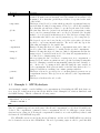
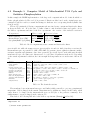
In this section we detail how to build and simulate the model illustrated in Figure 4.1 described in [6].
This model includes two compartments: Two reactions occur in the top compartment, ATP hydrolysis
and the creatine kinase (CK) reaction. Protons (H+ ) and adenine nucleotides (ATP4− and ADP3− ) are
transported between the two compartments via the F1 F0 -ATPase and the adenine nucleotide translocase
(ANT), which are described in the transporter database.
To build the model, we construct the following BSL file (‘Example2.bsl’) that defines two compartments, labeled cytoplasm and matrix:
compartment cytoplasm
ATPASE E.ATPASE.0
CK E.CK.0
compartment
matrix
0.8425 0.4970
0.6514 0.2106
transport
cytoplasm
matrix
ANT
T.ANT.1
F1F0ATPASE T.F1F0ATPASE.0
EOF
Again, there are no global model parameters. The first line defines a compartment called ‘cytoplasm’
with water content 0.8425 mL water/(mL cytoplasm) and fractional volume 0.4970 mL cytoplasm/(mL
cardiac tissue). Please note that the users may define water content and volume fraction values in an
alternative way, as long as it is consistent with the units of reaction/transport fluxes and reactant concentrations in different compartments. The enzymes ATPASE and CK are specified in this compartment.
A second compartment called ‘matrix’ is defined after the list of enzymes belonging to the compartment
19
‘cytoplasm’. There are no non-transport reactions defined in this compartment. The transport line in the
BSL file defines a list of transporters between the cytoplasm and matrix compartments.
transport
cytoplasm
matrix
The list of transporters that follow the transport declaration defines the ANT and F1F0ATPASE
transporters, with kinetic modules T.ANT.1 and T.F1F0ATPASE.0, respectively.
The BSL file can be used to generate an M-file model:
ModelInfo = BuildDXDT(’Example2.bsl’,’dXdT.m’);
The constructed M-file (dXdT.m), which is not listed here, has 265 lines. Thus even for a relatively
simple model, the utility generating complex code from relatively simple BSL-based declaration is apparent. The generated model can be simulated using the following commands.
%% Simulating Example 2
% (1.) Setting parameter values (no buffering)
B_X(1:2) = 1;
% Buffer capacity in both compartments
K_BX(1:2) = 1e-7;
% Buffer dissoc. constant in both compartments
T = 25;
% Temperature
% Enzyme and transporter activities:
par(1) = 0.1;
% k_ATPase (cytoplasm)
par(2) = 100.0;
% k_CK (cytoplasm)
par(3) = 1e-4;
% k_ANT
par(4) = 1e-3;
% F1F0 ATPase
par(5) = 1e-5;
% membrane capacitance
% (2.) Setting initial values
xo(1) = 10e-3; % ATP_cytoplasm
xo(2) = 0; % ADP_cytoplasm
xo(3) = 0; % Pi_cytoplasm
xo(4) = 10e-3; % phosphocreatine_cytoplasm
xo(5) = 10e-3; % creatine_cytoplasm
xo(6) = 0;
% ATP_matrix
xo(7) = 10e-3; % ADP_matrix
xo(8) = 5e-3; % Pi_matrix
xo(9) = 1e-7; % h_cytoplasm
xo(10) = 1e-3; % m_cytoplasm
xo(11) = 100e-3; % k_cytoplasm
xo(12) = 1e-7; % h_matrix
xo(13) = 1e-3; % m_matrix
xo(14) = 100e-3; % k_matrix
xo(15) = 0; % DPsi_cytoplasm_to_matrix
% (3.) Running for 15-second time course
[t,x] = ode23s(@dXdT,[0 60],xo,[],T,B_X,K_BX,par);
figure(1); plot(t,x(:,15))
20
10
[ATP]cytoplasm
Concentration (mM)
8
6
4
2
[ADP]cytoplasm
0
0
10
20
40
60
80
Time (sec)
100
120
20
40
60
80
Time (sec)
100
120
140
120
[ADP]matrix
100
6
ΔΨ (mV)
Concentration (mM)
8
4
80
60
40
2
[ATP]matrix
20
0
0
20
40
60
80
Time (sec)
100
0
0
120
Figure 4.1: Example 2: Top left shows the two-compartment system with ATP hydrolysis, F1 F0 -ATPase,
adenine nucleotide translocase (ANT), and creatine kinase (CK). This model is built from the BSL file
‘Example2.bls’, as described in Section 4.1. Top right and bottom left show the time courses of ADP and
ATP in the matrix and cytoplasm respectively. Bottom right shows the time course of the membrane
potential.
The simulated timecourses of several of the variables are illustrated in figure 4.1. In the initial state,
there is a concentration gradient driving ATP into the matrix and ADP out. An exchange of cytoplasmic
ATP for matrix ADP is associated with the reverse operation of the ANT transporter. Subsequent build-up
of ATP in the matrix leads to reverse operation of the F1F0-ATPase transporter. (The forward operation
direction is defined by the arrow directions in the model diagram in the top left panel of 4.1). ANT and
F1F0-ATPase operating in reverse mode both lead to a net transfer of positive charge from the matrix side
to the cytoplasmic side of the membrane, resulting in an increase in ΔΨ, which is defined as the potential
difference, cytoplasm potential minus matrix potential. Eventually, as ATP is consumed in the cytoplasm,
the membrane potential begins to diminish.
21
4.2
Example 3: Computer Model of Mitochondrial TCA Cycle and
Oxidative Phosphorylation
In this example the BISEN implementation of the large scale computational model of mitochondrial oxidative phosphorylation by Wu et al. [9] is presented. Kinetic modules based on the original paper were
constructed and the reaction, reactant and transport databases were set up using thermodynamic data
from [9] and [1].
The model contains the following compartments and associated water contents and fractional volumes
as shown in Table 4.1. Wc is the ratio of buffer volume to mitochondrial volume and equal to 80 for
the LaNoue experiments and 800 for the Bose experiments. An overview of the included reactions is
Compartment
Matrix (matrix)
Intermembrane Space (IM)
Cytoplasm/Buffer (cytoplasm)
Water content
water
0.6514 ( mL
mLmito )
mLwater
0.0724 ( mLmito )
mLwater
1.0 ( mL
)
buf f er
Fractional volume
mito
1/(1 + Wc ) ( mL
mLtotal )
mLmito
1/(1 + Wc ) ( mLtotal )
mito
Wc /(1 + Wc ) ( mL
mLtotal )
Table 4.1: Model compartments, water contents and fractional volumes
given in table 4.2, while the transporters are given in tables 4.3 and 4.4. Aside from these reactions, the
intermembrane space is permeable to ADP, ATP, AMP, Pi, pyruvate, citrate, alpha-ketoglutarate, malate,
succinate, aspartate and glutamate. Since these permeable species all depend on the same mitochondrial
membrane area per cell volume ratio, this was set to be a global model parameter in the model. Depending
on the actual experimental conditions, the ionic strength and temperature are set at the start of the model
file.
Reaction
Pyruvate Dehydrogenase
Citrate Synthase
Aconitatse
Isocitrate Dehydrogenase
α ketoglutarate dehydrogenase
Succinyl-CoA synthetase
Succinate dehydrogenase
Fumarase
Malate Dehydrogenase
Nucleoside Diphosphokinase
Aspartate Aminotransferase
Hexokinase
Adenylate kinase
Abbrev
PDH
CTS
ACON
IDH
AKGDH
SCS
SDH
FUM
MDH
NDK
AAT
HK
AK
Stoichiometry
pyruvate + COAS + NAD + H2O CO2tot + acetylcoA + NADH + H
acetylcoA + oxaloacetate + H2O COAS + citrate + 2 H
citrate isocitrate
isocitrate + NAD + H2O ketoglutarate + NADH + CO2tot + 2 H
ketoglutarate + COAS + NAD + H2O CO2tot + succinylcoA + NADH + H
succinylcoA + GDP + Pi succinate + GTP + COAS + H
succinate + coQ coQH2 + fumarate
fumarate + H2O malate
malate + NAD oxaloacetate + NADH + H
GTP + ADP GDP + ATP
ketoglutarate + aspartate oxaloacetate + glutamate
glucose + ATP glucose6phos + H
2 ADP ATP + AMP
Table 4.2: The chemical reactions
The membrane between intermembrane space and buffer is fully permeable to protons, potassium and
magnesium. CO2 is clamped in the matrix. Magnesium and potassium are clamped in the buffer, which
causes them to be clamped in the intermembrane space as well (due to the permeate command). In a
similar manner, oxygen is clamped in the entire model.
This leads to the following BSL file for the LaNoue experiments (‘Example3 LaNoue.bsl’):
temperature 28
% Global model parameters
22
Name
Pyruvate/H+ co-transporter
Glutamate/H+ co-transporter
Citrate/Malate anti-transporter
Ketoglutarate/Malate anti-transporter
Malate/Pi MALPI anti-transporter
Aspartate/H-Glutamate anti-transporter
Succinate/Malate anti-transporter
Adenine Nucleoside Translocate
Abbreviation
PYRH
GLUH
CITMAL
AKGMAL
MALPI
ASPGLU
SUCMAL
ANT
Out
pyruvate + H
glutamate + H
citrase
malate
malate
glutamate
succinate
ADP
In
malate
ketoglutarate
pi
aspartate
malate
ATP
Table 4.3: Transporters that merely transport and do not alter the transported species
Name
Complex I
Complex III
Complex IV
F1F0 ATPase
Abbreviation
ETC1
ETC2
ETC3
F1F0 ATPase
Transport
N ADHin + Qin + 5Hin N ADin + QH2,in + 4Hout
QH2,in + 2cytotoxout + 2Hin Qin + 2cytocredout + 4Hout
2cytocredout + 0.5O2,aq,in + 4Hin 2cytoredout + H2 O + 2Hout
+
ADPin + P iin + 3Hout
+ Hin AT Pin + H2 Oout + 3Hin
Table 4.4: Transporters that do alter the species involved
% mito membrane area per cell volume micron^{-1};
gamma = 5.99;
% minimal parameter value
MinCon = 0;
compartment
matrix
0.6514 1/81
PDH
E.PDH.1
CTS
E.CTS.0
ACON
E.ACON.0
IDH
E.IDH.0
AKGDH
E.AKGDH.0
SCS
E.SCS.0
SDH
E.SDH.0
FUM
E.FUM.0
MDH
E.MDH.0
NDK
E.NDK.0
AAT
E.AAT.0
clamped CO2tot
compartment
HK
cytoplasm 1 80/81
E.HK.1
clamped M
clamped K
23
compartment
transport
im 0.0724
1/81
im matrix
F1F0ATPASE
PYRH
GLUH
CITMAL
AKGMAL
MALPI
SUCMAL
ASPGLU
ETC1
ETC3
ETC4
PIH
KH
ANT
HLEAK
T.F1F0ATPASE.0
T.PYRH.0
T.GLUH.0
T.CITMAL.0
T.AKGMAL.0
T.MALPI.0
T.SUCMAL.0
T.ASPGLU.0
T.ETC1.0
T.ETC3.0
T.ETC4.0
T.PIH.1
T.KH.0
T.ANT.0
T.HLEAK.0
clamped O2aq
transport
cytoplasm im
PYRPERM
CITPERM
MALPERM
AKGPERM
SUCPERM
GLUPERM
ASPPERM
FUMPERM
ICITPERM
ADPPERM
ATPPERM
AMPPERM
PIPERM
T.PYRPERM.0
T.CITPERM.0
T.MALPERM.0
T.AKGPERM.0
T.SUCPERM.0
T.GLUPERM.0
T.ASPPERM.0
T.FUMPERM.0
T.ICITPERM.0
T.ADPPERM.0
T.ATPPERM.0
T.AMPPERM.0
T.PIPERM.0
permeate H
permeate K
permeate M
EOF
Analogous to [9] datasets from two independent experiments were used to determine the unknown
model parameters. The LaNoue et al. [4] data were measured from isolated rat heart mitochondria in
24
resting (state 2) and active state (state 3) with pyruvate and malate or only pyruvate as substrates. The
Bose et al. [3] data were measured from isolated pig heart mitochondria in state 2 and 3, using glutamate
and malate as substrates. The temperature and buffer volume are not the same in both experiments therefore both experiments need separate BSL files (‘Example3 LaNoue.bsl’ and ‘Example3 Bose.bsl’, respectively). One can build and carry out both models by running the matlab files Example3 LaNoue state2.m,
Exmaple3 LaNoue state3.m, and Example3 Bose state23.m.
4.2.1
Interacting with large scale models
Since large scale models tend to involve many parameters, it is wise to use the routines for managing parameters supplied with the BISEN package. When a model is built a MATLAB mat file is also generated.
This file contains a structure named modelInfo. This structure relates internal parameters, state variables
and flux indices to their respective names in the model by storing their indices. Using the routine setParameter enables the user to set and reference model parameters by name rather than index. When the
number of parameters of a submodel change, users will not need to shift parameters or initial conditions
around since the modelInfo structure changes accordingly.
For example, setting the pyruvate concentration in the buffer to 2 mM can be done as follows:
x0 = setParameter( x0, modelInfo.SVarID, ’pyruvate_cytoplasm’ ,
2e-3 );
Unspecified parameters can be set in an analogous manner. The activity of hexokinase is an unspecified
parameter named x HK in the hexokinase submodel. The following line of code turns off hexokinase
activity:
params = setParameter( params, modelInfo.ParID, ’x_HK’, 0 );
If the parameter does not exist, this function will display a warning, but not break execution. Obtaining
the value of a specific parameter, flux or state variable can be done manually using the modelInfo structure.
For example, obtaining the pyruvate concentration in the cytoplasm from a solution vector x can be done
as follows:
pyr = x( :, modelInfo.SVarID.pyruvate_cytoplasm );
If one wishes to store a whole set of parameters in the form of a human readable M-file the routine
generateParameterSet can be used. This uses the modelInfo structure, and a user supplied vector to
generate a m-file which returns the parameter or initial condition vector as output.
To obtain fluxes one needs to simulate the system in a first step and then use the result of such a
simulation to compute the internal fluxes. When additional export parameters are specified in the BSL
file, then the values of these during simulation can be acquired in a similar manner. The following code
shows how to obtain the complex IV flux. Here t and x are the time vector and state variable matrix (the
solution matrix).
for a = 1 : length( t )
[y,J(a,:)] = dXdT( t(a), x(a,:).’, T, BX, K_BX, params );
J_ETC4(a) = J( a, modelInfo.FluxID.ETC4_im_to_matrix );
end
The ’.mat’ file is useful in the sense that one does not need to rebuild the model every time MATLAB
is restarted. Simply loading the ’.mat’ file will supply the user with the modelInfo structure.
25
4.2.2
Simulating the experiments
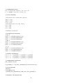
To be able to simulate the experiment, the simulation files used in the original paper were ported to
the new framework. These are heavily commented and available in the files Example3 LaNoue state2.m,
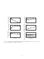
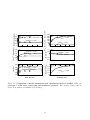
Exmaple3 LaNoue state3.m, and Example3 Bose state23.m. As shown in 4.2, 4.3 and 4.4, the model simulations reproduce both sets of experiments quite well.
26
Aside from the differences in physicochemical constants, a few notable differences between the two
model implementations are listed in table 4.5.
BISEN implementation
pH held constant by large proton buffer
Temperature correction of metabolite Gibbs energy of formation and pKa’s done separately for
both experimental temperatures
Redundant state variables present
Implementation according to [8]
pH clamped
No temperature correction of the metabolite
Gibbs energy of formation and pKa’s for different experimental temperatures.
Some state variables derived off of total concentration pools.
Table 4.5: Differences between implementations of the model of the TCA cycle and oxidative phosphorylation
4.3
Conserved pools
Reaction stoichiometry imposes a constraint on the system, namely that of conserved pools. Conserved
pools always appear as linearly dependent rows in the stoichiometry matrix. Checking the conserved pools
can be beneficial to diagnose problems with the model. The absence of expected conserved pools can
indicate a problem, while fluctuations of pools that should have been conserved can indicate unadequate
solver accuracy.
To be able to check the conserved pools, the conservation matrix of the system is computed in the
builder according to the method proposed by [5]. To be able to use this matrix one can use the command
checkPools. If supplied with the modelInfo matrix, this command gives a list of conserved pools. Supplying
the routine with a solution matrix results in an actual estimation of the conserved pool concentration, based
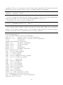
on the summation of its constituents.
checkPools( modelInfo );
For example, after running example 2, one can use the following line of code to inspect the list of conserved
pools and their respective time course (which should be constant).
checkPools( ModelInfo, x, 1, t );
The command, aside from the graphs produced outputs a list of pools and their respective concentration.
As shown below, these concentrations correspond to the initial pool concentrations.
Pool 1 (Avg value: 0.02, Max change: 3.469e-018)
phosphocreatine_cytoplasm
creatine_cytoplasm
Pool 2 (Avg value: 0.01, Max change: 1.735e-018)
ATP_cytoplasm
ADP_cytoplasm
Pool 3 (Avg value: 0.01, Max change: 1.735e-018)
ATP_matrix
ADP_matrix
Pool 4 (Avg value: 0.025, Max change: 6.536e-015)
ATP_cytoplasm
27
ATP_matrix
Pi_cytoplasm
phosphocreatine_cytoplasm
Pi_matrix
Max pool change: 6.53644e-015
28
A
400
200
0
60
C
40
total
[AKG]
[MAL]total (nmoles/mg)
[GLU]total and [ASP]total (nmoles/mg)
[SUC]total (nmoles/mg)
[CIT]buffer and [CIT]total (nmoles/m
600
(nmoles/mg)
[PYR]total (nmoles/mg)
800
20
0
2000
1500
E
1000
500
0
0
100
200
300
Time (sec)
400
500
30
B
20
10
0
30
D
20
10
0
15
F
10
5
0
0
50
100
150
Time (sec)
200
250
Figure 4.2: Comparison of model simulations to state-2 kinetic data. Here measured data points
are shown along with model simulations (solid lines).
29
400
total
200
0
90
[SUC]
(nmoles/mg)
[GLU]total and [ASP]total (nmoles/mg) total
[PYR]
A
600
[AKG]total (nmoles/mg)
[MAL]total (nmoles/mg)
[CIT]total (nmoles/mg)
(nmoles/mg)
800
0
E
1000
500
0
0
B
4
2
0
D
160
30
1500
6
240
C
60
2000
8
100
200 300
Time (sec)
400
500
80
0
15
F
10
5
0
0
50
100 150
Time (sec)
200
250
Figure 4.3: Comparison of model simulations to state-3 kinetic data. Here measured data points
are shown along with model simulations (solid lines).
30
0.8
A
MVO (mol O2 min−1 (mol Cyto A)
[ADP]buffer = 0 mM
0.6
[ADP]buffer = 1.3 mM
0.4
0.2
0
350
300
250
200
150
100
50
0
B
7.5
D
[ADP]buffer = 1.3 mM
[ADP]buffer = 0 mM
0.25
0.2
C
[ADP]
= 1.3 mM
[ADP]
= 0 mM
buffer
0.15
buffer
0.1
Matrix pH
2
NADH (Normalized)
0.05
= 1.3 mM
[ADP]
= 0 mM
[ADP]
= 0 mM
buffer
6.75
6.5
E
[ADP]
buffer
190
= 0 mM
[ADP]buffer = 1.3 mM
170
150
130
0
[ADP]
buffer
7
0
210
ΔΨ (mV)
7.25
Matrix ATP/Atot
(Normalized)
2+
CytoC
1
2
4
6
Buffer [PI] (mM)
8
1
0.8
buffer
0.6
0.4
[ADP]buffer = 1.3 mM
0.2
0
0
10
F
2
4
6
Buffer [PI] (mM)
8
10
Figure 4.4: Comparison of model simulations with experimental data on NADH, M VO2 , cytochrome c redox state, matrix pH and membrane potential. Here measured data points are
shown along with model simulations (solid lines).
31
Chapter 5
Further Information
5.1
Where to Get BISEN
BISEN is available from the following location: http://bbc.mcw.edu/BISEN
5.2
Bug Reporting and Tracking
Please report bugs at the following location: http://bbc.mcw.edu/BISEN
5.3
Future Plans
This version of the builder is a first step in the direction of a thermodynamic framework for simulating
biochemical reactions. However, there is some work left to be done.
5.3.1
Additional ion binding
Currently, the framework is set up for 3 ions namely protons, magnesium and potassium. In the current
version the solution of the linear system of equations for computing the time derivatives of these ions is
hard coded. In the future, it could be possible to incorporate an automatic solver for these equations in the
builder to automatically compute the ion equations for 4 or more ions. This way Ca2+ and N a+ could be
taken into account. Additional ion binding could be implemented by using the MATLAB symbolic toolbox
to generate the actual expressions or by using an implementation of Cramer’s rule.
5.3.2
Model reduction
Many models contain conserved pools or moieties. A conserved pool effectively means that one of the
variables of the pool is redundant and can be replaced by a linear combination of the other variables. It
is worth investigating whether such a reduction in state variables improves computational performance of
the generated models.
Furthermore, the ’permeate’ command specifies the permeation of two compartments. When this
occurs, only one of the state variables actually has a value associated with it. In the current version the
redundant state variable is not removed from the state variable vector.
32
Chapter 6
Thermodynamics of biochemical
reactions
This section gives a very brief overview of the thermodynamics involved in biochemical reactions. It is
based on the theory in [2], [1] and [7].
6.1
Definitions
To be able to treat the theory unambiguously, the following definitions are used throughout this report. A
reactant (e.g. ATP) is basically a compound that can be subdivided into species with a specific binding
(e.g. M gAT P 2− , AT P 4− , HAT P 3− etc). A biochemical reaction is a reaction mechanism that is not
stoichiometrically balanced in terms of mass or charge (6.1).
AT P ADP + P I
(6.1)
A reference reaction however is stoichiometrically balanced (6.2).
AT P 4− + H2 O ADP 3− + HP O42− + H +
6.2
(6.2)
NPT Ensemble
Biochemical reactions in a biological system are best understood in a constant pressure setting, hence the
choice of the NPT ensemble is made. The relative probability of a state in the NPT system is expressed
in terms of enthalpy (6.3). Here H represents the enthalpy, T the temperature, P the pressure and μ the
chemical potential.
dH = T dS − V dP + μdN
(6.3)
The probability law for an NPT system is given by (6.4).
e−βH
Z
e−βHi
Z=
P =
i
33
(6.4)
(6.5)
The average enthalpy of the NPT system is computed as (6.6). And the Gibbs free energy is defined as
G=E-TS+PV or G=H-TS.
−βHi
δ
δ
i Hi e
= − ln[
e−βHi ] = − lnZ.
(6.6)
H= −βH
i
e
δβ
δβ
i
i
H = G − T(
∂ G
∂(G/T )
∂G
)N,V = −T 2 [
( )]N,V = [
]N,V
∂T
∂T T
∂(1/T )
(6.7)
Using the manipulation briefly outlined in (6.7) it can be derived that the Gibbs free energy can be expressed
as (6.8). Hence a system that minimizes the Gibbs free energy, maximizes Z (probability weighted sum of
states). NPT systems thrive to decrease G.
G = −kB T lnZ
(6.8)
A general chemical reaction can be expressed in terms of species Ai and stoichiometric coefficients νi .
Negative stoichiometric coefficients refer to reactants, while positive ones refer to products. For example
for (6.9), the stoichiometric coefficients would be ν1 = −5, ν2 = 4 and ν3 = 2.
5A1 4A2 + 2A3
(6.9)
Hence the associated change in Gibbs free energy at constant temperature and pressure would be (6.10)
where φ represents the number of times the reaction has progressed. Based on this equation, definition
(6.11) is made.
Ns
νi μi dφ
(6.10)
(dG)P,T =
i=1
s
dG
)P,T =
νi μ i
dφ
N
Δr G = (
(6.11)
i=1
If one assumes that the molecules do not interact in such a way that the energy associated with a given
conformation of one molecule is influenced by the conformation of another molecule in the system then the
following expression can be derived for μ (6.12) leading to the expression shown in (6.13). Using Avogadro’s
constant this can be expressed as (6.14) where Δr G0 is given by (6.15) where Δf G0i is the free energy of
formation of species i at a specific temperature, pressure and ionic strength.
μ = μ0 + kB T ln
Δr G = Δr G0 +
Ns
[C]
[C0 ]
Ns
νi RT ln
i=1
Δr G0 =
Ns
[C]i
[C]0
(6.13)
[C]i
[C]0
(6.14)
νi kB T ln
i=1
Δr G = Δr G0 +
(6.12)
νi Δf G0i
(6.15)
i=1
At equilibrium Δr G equates to zero, which results in the well known expression (6.16) for the equilibrium
constant.
Ns
[C]i νi
0
(
)
(6.16)
Keq = e−Δr G /RT =
[C]0
i=1
34
Fluxes obey the relationship given in (6.17).
ΔG
J+
= e RT
−
J
6.3
(6.17)
Electrophysiology
Another important phenomenon in biological reactions is the electrostatic potential across cell membranes.
The thermodynamic potential of a chemical process with movement of charge across a membrane is given
by (6.18). Here zi denotes the valence of the charged species, νi the number of ions transported and ΔΨ the
electrostatic potential difference between the two compartments separated by the membrane. Furthermore,
Nc and kB are the Coulomb and Boltzmann constants.
Δμ = Δμ0 +
ΔΨ
Nc
νi zi + kB T
νi ln[C]i
(6.18)
i∈inside
Similar to the derivation of (6.14), the equation for the Gibbs free energy can be written as (6.19) and
the apparent equilibrium becomes (6.20). In this equation F is the Faraday constant which is defined as
the Avogadro constant divided by the Coulomb constant.
Δr G = Δr G0 +
Ns
νi RT ln
i=1
Keq = e−Δr G
[C]i
+ F ΔΨ
νi zi
[C]0
(6.19)
i∈inside
0 /RT − F ΔΨ
RT
=
Ns
[C]i νi
(
)
[C]0
(6.20)
i=1
The biological membrane itself is treated as a capacitor with constant capacitance, leading to the following expression for the membrane potential (ΔΨ) (6.21). This equation assumes a linear current/voltage
relationship and can be used to calculate the change in membrane potential using the charge fluxes across
the membrane.
dΔΨ
=−
Ioutward
(6.21)
Cm
dt
6.4
Proton and ion binding
Tabulated versions of the equilibrium constant of a reaction are valid for a specific defined state ([H2 O =
55.5M and pH = 7]. These concentrations are implicitly incorporated in the standard Gibbs energies. In
an in vitro system however, pH is often not constant. Nor are ion concentrations in the solution. Therefore
the framework needs to take proton and ion binding into account.
The state with i protons bound to reactant L shall be referred to as [LHi ]. Considering only proton
binding, the total concentration of L is given by (6.22) and the concentration of L with just one protonation
is given by (6.23). Here K1 denotes the dissociation constant.
[L] =
N
[LHi ]
(6.22)
i=0
[LH1 ] = [LH0 ]
35
[H + ]
K1
(6.23)
Iteratively accounting for N protonations leads to the general equation (6.24).
[H + ]i
[LHi ] = [LH0 ] j≤i Kj
(6.24)
The total concentration is then given by (6.25), which relates the total concentration with the least
protonated form of the reactant. This conversion is known as the binding polynomial. In this framework,
the model state variables correspond to the reactants, the sum of all species. Therefore the amount of
proton-bound ATP can be computed as (6.26), where [AT P ] corresponds to the model state variable.
[L] = [LH0 ](1 +
N
[H + ]i
) = [LH0 ]PL ([H + ])
K
j
j≤i
(6.25)
i=1
[HAT P 3− ] =
[H + ]
[AT P ]
AT P
PAT P ([H + ]) KH
(6.26)
Calculating the Keq for the reaction shown in (6.27) results in expression (6.28) with Δr G0 the Gibbs
free energy change for the reaction.
AT P 4− + H2 O ADP 3− + HP O42− + H +
Keq = e
−Δr G0
RT
=(
[ADP 3− ][HP O42− ][H + ]
[ADP ][P I][H+]
PAT P ([H + ])
)
)
=
(
eq
eq
[AT P 4− ]
[AT P ]
PADP ([H + ])PP I ([H + ])
(6.27)
(6.28)
This expression can be written in terms of reactant concentrations (in this case [AT P ], [P I] and [AT P ],
which are state variables) using the binding polynomials. Equation (6.17) can then be used to relate the
forward to the backward flux.
Keq = (
[ADP ][P I]
PADP ([H + ])PP I ([H + ])
)eq = Keq
[AT P ]
[H + ]PAT P ([H + ])
(6.29)
This method can be extended to account for multiple ion binding by generalizing the binding polynomial
to the expression given in (6.30). Here [Mlzl + ] corresponds to any ion.
N
P ([H
+
z +
], [Mj j ])
Ml
NH
n
ions [Mlzl + ]i
[H + ]i
=1+
+
j≤i Kj
j≤i KMl ,j
i=1
l
(6.30)
i=1
To be able to account for proton and ion binding, one needs to have their respective concentrations.
To be able to obtain an expression for this concentration one needs to consider mass conservation. The
conservation of metal ions can be written as (6.31).
z +
z +
z +
z +
j
j
] = [Mj,fj ree ] + [Mj,bound
] + [Mj,fj lux ]
[Mj,total
(6.31)
While the conservation of protons can be expressed as (6.32). Here [H + ]ref erence denotes the protons
present in the reference species and [Hf+lux ] the flux into the compartment.
+
+
+
+
] = [Hf+ree ] + [Hbound
] + [Href
[Htotal
erence ] + [Hf lux ]
(6.32)
Differentiation with respect to time results in equation (6.33).
0=
d[Hf+ree ]
dt
+
+
+
+
d[Hbound
] d[Href erence] d[Hf lux ]
+
+
dt
dt
dt
36
(6.33)
Using the chain rule, the second term can be expanded into (6.34) leading to an equation depending
on both the cation as well as the species derivatives.
+
+
+
∂[Hbound
]
] d[H + ] ∂[Hbound
] d[Mj
d[Hbound
=
+
z
+
+
j
dt
∂[H ]
dt
dt
∂[M ]
zj +
]
+
∂[H +
bound ] d[Li ]
j
j
∂[Li ]
i
dt
(6.34)
The reference term is based on the proton stoichiometry of the individual reactions and the respective
flux of that reaction (6.35).
+
Nreactions
d[Href
erence ]
=−
nk Jk
(6.35)
dt
k=1
The flux term corresponds to the proton flux into the current compartment JtH . Substituting the expanded terms and rearranging equation (6.33) results in differential equations for the proton concentration
(6.36). A similar approach can be used to obtain the differential equations governing the ion concentration
(6.37).
d[H + ]
dt
−
Nions
j
z +
j
+
∂[Hbound
] d[Mj ]
z +
dt
∂[M j ]
−
Nspecies
+
] d[Li ]
∂[Hbound
dt
∂[Li ]
i
j
=
dt
−
Nions
l
z +
z +
j
] d[M j ]
∂[Mj,bound
l
zj +
dt
∂[M
]
−
l
=
Nreactions
k=1
nk Jk + JtH
(6.36)
+
∂[Hbound
]
δ[H + ]
1+
z +
d[Mj j ]
+
Nspecies
i
z +
j
] d[Li ]
∂[Mj,bound
dt
∂[Li ]
z +
1+
j
∂[Mj,bound
]
+ JtH
(6.37)
z +
δ[Mj j ]
If all the terms are known, then these equations can be solved as a linear system of equations to
obtain the uncoupled time derivatives of the protons and ions. Under the assumption that ion binding is a
rapid equilibrium process one can write the terms in front of the time derivatives in terms of dissociation
constants, reactant concentrations and binding polynomials. If one assumes higher order binding negligible
by choosing the reference state appropriately for the physiological range then the resulting terms will
z +
become (6.38) to (6.42). Here [Mj j ] corresponds to the concentration of ion M zj + .
+
]
∂[Hbound
z +
∂[Mj j ]
=−
Nreactants
[Li ][H + ]
KiH
i=1
Ki j (Pi ([H + ], [Mxzx + ]))2
+
]
∂[Hbound
=−
∂[H + ]
M
Nreactants
i=1
[Li ](1 +
nions
z +
[Mj j ]
j=1
(6.38)
M
)
Ki j
KiH (Pi ([H + ], [Mxzx + ]))2
(6.39)
z +
zj +
]
∂[Mj,bound
+
∂[H ]
=−
[Li ][Mj j ]
Nreactants
Mj
Ki
KiH (Pi ([H + ], [Mxzx + ]))2
i=1
(6.40)
z +
zj +
]
∂[Mj,bound
∂[Mkzk + ]
=−
[Li ][Mj j ]
Nreactants
i=1
Mj
Ki
KiMk (Pi ([H + ], [Mxzx ]))2
37
(6.41)
zj +
∂[Mj,bound
]
zj +
∂[Mj ]
=−
Nreactants
i=1
nions
z +
[Ml l ]
l=j
K Ml )
KlH (Pi ([H + ], [Mxzx + ]))2
[Li ](1 +
(6.42)
Where the binding polynomial accounting for first order bindings only (6.43) is based on the general
expression (6.30).
[H + ] Mj
=1+ H +
.
Mj
Ki
j K
zj +
P ([H
+
], [Mxzx + ])
(6.43)
i
In the present work, the system is set up for 3 ions namely H + , K + and M g2+ .
6.5
Temperature and ionic strength dependence
As mentioned earlier, the change in Gibbs energy of a reaction can be calculated according to (6.44).
Similarly the change in enthalpy can be calculated according to (6.45).
0
Δr G =
Ns
νi Δf G0i
(6.44)
νi Δ f H i
(6.45)
i=1
Δr H =
Ns
i=1
Assuming that the enthalpy is independent of temperature (which is reasonable over the physiological
range [1]), then the binding affinities can be temperature corrected by means of the enthalpy of the involved
reactants (6.46).
Δr H 0 (T2 − T1 )
KT
(6.46)
ln 2 =
KT1
RT1 T2
1
Using the definition of pKa (6.47) and the fact that log10
(e) = 2.3026, this equation can be rearranged into
(6.48).
(6.47)
pKa = −log10 (Ka )
pKaT2 = pKaT1 + (
1
1 Δr H 0
− )
T2 T1 2.3026R
(6.48)
The effects of ionic strength on pK can be approximated using the relation (6.49). Here
to the change in zi2 due to the dissociation.
1
pKaI2
νi zi2 refers
1
I12
αK
I22
(
= pKaI1 +
−
)
νi zi2
1
2.303 1 + 1.6I 12
2
1 + 1.6I2
1
(6.49)
αK = 1.10708 − 1.54508 ∗ 10−3 T + 5.95584 ∗ 10−6 T 2
(6.50)
The enthalpy itself is also a function of the ionic strength of the solution. The effect of ionic strength
can be described by the following empirical equation (6.51).
1
0
0
Δr H = Δr H (I = 0) +
αH I 2
vi zi2
1 + 1.6I
1
2
38
= Δr H 0 (I = 0) + βH (T, I)
vi zi2
(6.51)
αH = −1.28466 ∗ 10−5 T 2 + 9.90399 ∗ 10−8 T 3
(6.52)
1
βH =
αH (T )I 2
(6.53)
1
1 + 1.6I 2
The free energy of formation also depends on ionic strength. This dependence is approximated by
(6.54).
1 αG I 2
νi zi2
0
0
0
=
Δ
G
(I
=
0)
−
β
(T,
I)
νi zi2
(6.54)
Δr G = Δr G (I = 0) −
r
G
1
2
1 + 1.6I
αG = RT αK = 9.20483 ∗ 10−3 T − 1.28467 ∗ 10−5 T 2 + 4.95199 ∗ 10−8 ∗ T 3
(6.55)
1
βG =
αG (T )I 2
1
(6.56)
1 + 1.6I 2
These empirical formulas are based on the assumption that the heat capacities are zero [1].
The effect of temperature on the Gibbs energy, assuming that the enthalpies are approximately constant
is given by (6.57) [2]. Due to the linearity, one can substitute the reaction enthalpy and reaction Gibbs
energy change in this equation.
T2
T2
0
(6.57)
Δf Hi0 + Δf G0i (T1 )
Δf Gi (T2 ) = 1 −
T1
T1
6.6
Carbon dioxide
Carbon dioxide does not significantly bind to metal ions or protons itself, but can be hydrolyzed to H2 CO3
via the reaction (6.58). Protons can dissociate from H2 CO3 .
CO2 + H2 O H2 CO3
(6.58)
It is convenient to express apparent thermodynamic properties in terms of total CO2 , which is defined as
(6.59)
(6.59)
[
CO2 ] = [CO2 ] + [H2 CO3 ] + [HCO3− ] + [CO32− ]
Writing down the expression
containing the binding polynomial for carbon dioxide leads to (6.60), where
it can be seen that
CO2 is expressed in terms of [CO32− ].
[H + ] [H + ]2
[H + ]2
+
+
)
[
CO2 ] = [CO32− ](1 +
K1
K1 K2 Kh K1 K2
(6.60)
Here Kh refers to the formation of H2 CO3 from water and carbon dioxide. Because of the fact that the
total carbon dioxide is now expressed in terms of [CO32− ], the water and protons involved need to be taken
into account in terms of stoichiometry.
For the reaction (6.61) this would lead to the sum of (6.62) and (6.63), which is given by (6.64).
(6.61)
A
B+
CO2
A B + CO2
(6.62)
CO2 + H2 O CO32− + 2H +
(6.63)
A + H2 O B + CO32− + 2H +
(6.64)
39
Bibliography
[1] R. A. Alberty. Thermodynamics of Biochemical Systems. John Wiley & Sons, Hoboken, NJ, 2003.
[2] D. A. Beard and H. Qian. Chemical Biophysics: Quantitative Analyis of Cellular Systems. Cambridge
University Press, Cambridge, UK, 2008.
[3] S. Bose, S. French, F. J. Evans, F. Joubert, and R. S. Balaban. Metabolic network of oxidative
phosphorylation: multiple roles of inorganic phosphate. J. Biol. Chem., pages 39155–39165, 2003.
[4] K. LaNoue, W. J. Nicklas, and J. R. Williamson. Control of citric acid cycle activity in rat heart
mitochondria. J. Biol. Chem., 245:102–111, 1970.
[5] Ravishankar Rao Vallabhajosyulaa, Vijay Chickarmanea, and Herbert M. Sauroa. Conservation analysis
of large biochemical networks. Bioinformatics, pages 346–53, ’2006.
[6] J. Vanlier, F. Wu, F. Qi, K. Vinnakota, Y. Han, R.K. Dash, and D.A. Beard. BISEN: Biochemical
Simulation Environment. Bioinformatics, 2009.
[7] K. C. Vinnakota, F. Wu, M. J. Kushmerick, and D. A. Beard. Multiple ion binding equilibria, reaction
kinetics and thermodynamics in dynamic models of biochemical pathways. Methods Enzymol., 454:29–
68, 2009.
[8] F. Wu, J. A. Jeneson, and D. A. Beard. Oxidative ATP synthesis in skeletal muscle is controlled by
substrate feedback. Am. J. Physiol., 292:C115–C124, 2007.
[9] F. Wu, F. Yang, K. C. Vinnakota, and D. A. Beard. Computer modeling of mitochondrial tricarboxylic
acid cycle, oxidative phosphorylation, metabolite transport, and electrophysiology. J. Biol. Chem.,
282:24525–24537, 2007.
40