Download ITC Expert User`s Manual

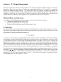
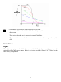
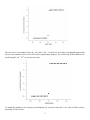
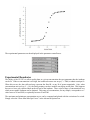
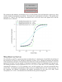
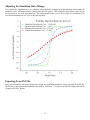
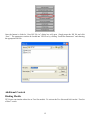
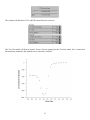
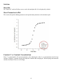
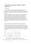
ITC Expert
User’s Manual
1
Section 1: ITC Expert Background........................................................................................................................ 3
Minimal Heats and Injections ............................................................................................................................. 3
C Parameter......................................................................................................................................................... 3
C Limitations ...................................................................................................................................................... 4
High C................................................................................................................................................................. 4
Low C.............................................................................................................................................................. 6
Concentrations Ratio........................................................................................................................................... 6
Section 2: ITC Expert Controls.............................................................................................................................. 7
The Experimental Design Wizard Walkthrough................................................................................................. 7
Starting the Wizard ......................................................................................................................................... 7
Experimental Boundaries................................................................................................................................ 8
When Heats are Too Low ............................................................................................................................... 9
Adjusting the Simulated Curve..................................................................................................................... 10
Adjusting the Simulation Out of Range........................................................................................................ 11
Exporting To an INJ File .............................................................................................................................. 11
Additional Controls........................................................................................................................................... 12
Binding Models ............................................................................................................................................. 14
Buttons .......................................................................................................................................................... 14
Switches ........................................................................................................................................................ 15
Section 3: Sample Considerations ....................................................................................................................... 16
Sample Preparation Recommendations ............................................................................................................ 16
Sample Solution Preparation............................................................................................................................. 16
Concentrating and Filtering Samples................................................................................................................ 17
Sample Concentration Measurement ................................................................................................................ 17
Temperature Dependence of Binding Heats ..................................................................................................... 17
Section 4: Troubleshooting .............................................................................................................................. 18
Why is my Isotherm too steep?......................................................................................................................... 18
Why does my Isotherm not look like a Sigmoid?............................................................................................. 18
Disclaimer: Simulated data from the ITC Expert software is not a
replacement for actual experimental runs on the VP-ITC.
2
Section 1: ITC Expert Background
ITC Expert will quickly and conveniently simulate an ITC binding experiment within the OriginTM 7.0 software
application. Based on a specific set of sample and experimental conditions, ITC expert will automatically
generate a simulated binding isotherm. ITC Expert then allows the operator to change the sample and
experimental conditions and the simulated binding isotherm will be appropriately updated to reflect those new
conditions. Finally, the ITC Expert utility will allow the operator to save the details of the experimental and
sample conditions so that they can be applied to a real experiment with the VP-ITC instrument.
Minimal Heats and Injections
To confidently fit the binding isotherm the experiment must meet the following conditions:
• Total heat of experiment is at least 50 µCal.
• Number of injections must be 10 or greater.
• The heat of the first injection must not be lower than 5 µCal.
C Parameter
The critical parameter which determines the shape of the binding isotherm is the unitless parameter C, which is
the product of the binding constant K times the total macromolecule concentration in the cell at the start of the
experiment, M, times the stoichiometry parameter, N.
C=K*M*N
Very large C values lead to very tight binding and the isotherm is nearly rectangular in shape, with the height
corresponding exactly to DH and with the sharp drop occurring precisely at the stoichiometric equivalence point
N in the molar ratio (Note: DH represents ΔH throughout manual). The shape of this curve is invariant with
changes in K so long as the C value remains above ca. 5000. As C is reduced by decreasing M (i.e., holding K,
DH and other parameters constant), the drop near the equivalence point becomes broadened and the intercept at
the Y axis becomes lower than the true DH. In the limit of very low initial M concentration (cf., C=0.1), the
isotherm becomes featureless and traces a nearly horizontal line indicative of very weak binding. It is apparent
from looking at these isotherms that their shape is reasonably sensitive to binding constant only for C values in
the range 10 < C < 3000, corresponding to binding of intermediate strength. We will refer to this range as the
"experimental K window". When available, the middle of the window from C = 50 to 500 is most ideal for
measuring K. The ITC Expert software utility will use C = 100 as the ideal situation for experimental design.
See the graph below for some example ‘C curves’.
3
XTOT
MTOT
= concentration of injected solute in the cell before each injection.
= concentration of macromolecule in the cell before each injection, after correction for volume
displacement.
The x-axis on the graph above is expressed in terms of Molar Ratio.
The correct choice of macromolecule concentration for an experiment depends upon the magnitude
of K.
C Limitations
High C
When C is too large (greater than 3000), the curvature in the binding isotherms for binding systems with
varying Ks, will no longer appear unique. Below is an isotherm where KA=109 and C=105. Notice how the
curve is nearly a step function.
4
The next curve is an isotherm where KA=1010 and C=106. C in this case is an order of magnitude greater than
the previous isotherm; however the curve has not significantly changed. We could easily fit this isotherm to a
model using KA=109, 1010, or even greater values.
To enable the isotherm to be accurately (and uniquely) fit, we need to keep the C at a value of 3000 or lower,
preferably at 500 or below.
5
Low C
When C is too low, the isotherms become too flat to be distinguishable. Keeping the C value above 10,
preferably 50 or higher, will ensure that the resulting binding isotherm is not featureless and that it can be
properly fit.
Concentrations Ratio
The syringe concentration should be approximately 15 times the cell concentration. The cell concentration is
the critical concentration of the two and it will be used to determine the syringe concentration. The cell
concentration will define the C value, but the syringe concentration (along with injection volume) will only
determine the spacing of points on the x-axis of the binding isotherm. Because of this, the concentration of the
syringe can really be anywhere from 10 to 20 times the concentration of the cell concentration. The ITC Expert
simulator sets the syringe concentration at 15 times the cell concentration, which is an appropriate choice for
your experiments.
6
Section 2: ITC Expert Controls
The Experimental Design Wizard Walkthrough
The ITC experimental design wizard is an automated program that will simulate and help to design a One Site
or Two Site ITC binding experiment. The program will use input guesses (N, K, and DH) to calculate the
proper concentrations, number of injections, and injection volumes. Through its algorithms, the wizard will
ensure that the ITC experiment produces at least 50 μCal of total energy, a minimum of 5 µCal of energy for the
first injection, and a desirable C value and binding isotherm shape that can be easily fit to the calorimetric
model. Once the simulation passes the necessary heat requirements, the isotherm is plotted in the simulator.
The example below describes a One Site binding model.
Starting the Wizard
To start the wizard, click on the Start Experimental Design Wizard Button.
This will open the Binding Parameters dialog box. You must enter guesses of N, K, and DH to initiate the
wizard.
The wizard will begin by setting C to 100, and solve for the macromolecule concentration. The program will
then determine the appropriate number of injections and injection volumes for the experiment and plot the
isotherm.
7
The experimental parameters are then displayed in the parameter control boxes.
Experimental Boundaries
The ability of the VP-ITC to collect quality data at a given concentration does not guarantee that the isotherm
can be fit. When a concentration is too high, the isotherm becomes too steep (C > 3000) to obtain a unique fit.
When this occurs, the data collected may represent the fitted K, or any K of greater magnitude. Also, when
concentrations are too low (C < 10), the fitting routines can have trouble converging on the data. This happens
because we have only collected data on the tail end of the isotherm. There exists a range of concentrations over
which an acceptable isotherm can be obtained. This range of concentrations, for any sample, corresponds to a C
value between 10 and 3000, or optimally between 50 and 500.
The maximum and minimum concentration curves can be computed and plotted with the activation of a switch.
Simply select the “Show Max/Min/Opt Curves” in the Advanced Options box.
8
The maximum and minimum concentration curves are then plotted (green and light blue respectively) along
with the simulated experimental curve (black). The fourth curve is the optimal curve (blue). The optimal curve
represents a C value of 100. By default, the simulated curve will be the same as the optimal curve until the
simulated curve is adjusted.
When Heats Are Too Low
We will define a good ITC experiment so that its isotherm has a C value between 10 and 3000, the total heat of
the experiment is at least 50 μCal, and the first injection is at least 5 µCal. During the simulation, the total heat
of the experiment is measured. If the total heat is less than 50 μCal, the concentrations are increased. If the first
injection is less than 5 µCal, the number of injections is decreased. Below is a simulation of an extreme case.
The binding parameters for this simulation were N of 1, K of 106 M-1, and a DH of -150 Cal/Mol/Deg. When
computing the isotherms at Cs of 10 (minimum conc.) and 100 (optimal conc.), the total experimental heats
were too low. In raising the concentrations of those curves to a minimal heat level, the 2 curves converge. In
this simulation, the minimal concentration and optimal concentration are the same (0.25 mM), which
corresponds to a C of 249. Concentrations lower than that do not generate enough heat.
9
Adjusting the Simulated Curve
Once the simulation curve has been created, every parameter can be adjusted. The simulated curve will then be
recalculated and plotted. If the experimental parameters (number of injections, injection volume, cell
concentration, or syringe concentration) are adjusted, the maximum, minimum, and optimal concentrations will
remain constant. If the binding parameters (N, K, and DH) are adjusted, the maximum, minimum, and optimal
concentrations will change accordingly. To adjust the parameters, simply click on the toggle arrows. K and
DH will increase and decrease by a half an order of magnitude of its current value.
10
Adjusting the Simulation Out of Range
If you adjust the simulation curve to a situation where the heats no longer meet the minimum requirement, the
simulation curve will turn red and a warning message will appear. This situation is most likely caused by too
few injections or too weak concentrations. The requirements for the curve to be in range are a total heat of 50
μCal and a minimum heat of 5 µCal in the first injection.
Exporting To an INJ File
Once you are satisfied with your experiment’s design, the simulation parameters can be exported as an INJ file.
An INJ file is an Experimental Parameters file used by VPViewer. To export to an INJ file simply click on the
“Export to INJ File” button.
11
Once the button is clicked a “Save INJ File As” dialog box will open. Simply name the INJ file and click
“Save”. The parameters can then be loaded into VPViewer by clicking “Load Run Parameters” and choosing
the appropriate INJ file.
Additional Controls
Binding Models
ITC Expert can simulate either One or Two Site models. To activate the Two Site model click on the “Two Set
of Sites” switch.
12
The controls will then show N, K, and DH control boxes for each site.
The Two Site model will then be plotted. Since C has no meaning for the Two Site model, the C control and
the maximum, minimum, and optimal curves will not be available.
13
Buttons
Start New Session
This button clears the simulation plot and allows the operator to start over in the simulation process.
Add New Curve
This button saves the current simulated curve to a temporary plot. A new simulation session will begin, with
the previous curve still plotted. This is ideal for comparing two different simulations.
Input New Bind. Parameters
This button allows user to jump to new binding parameters, without going through several iteration steps.
Input New Run Parameters
This button allows user to jump to new run parameters, without going through several iteration steps.
Print Simulation Plot
The Print button will print the simulation plot.
Export to DH File
This button exports a DH file. The DH file can then be imported into ITC data analysis and fit.
14
Switches
Show Kd
The “Show Kd” switch will allow users to work with and adjust Kd. Ka is displayed by default.
Show Parameters in Plot
This switch will past the binding parameters and experimental parameters to the simulation plot.
Constant C or Constant Concentrations
Since C is proportional to K and concentrations, when adjusting K, either C or concentrations must be kept
constant. Keeping C constant will keep the shape the constant while changing K. When keeping concentrations
constant, the shape of the curve will change.
15
Section 3: Sample Considerations
Sample Preparation Recommendations
Care in preparation of samples for use in the Isothermal Titration Calorimeter (ITC) is critical to the overall
quality of the binding experiment. Three aspects of the preparation are of particular importance: matching of
component buffers, concentrating the experimental samples, and accuracy of the input sample concentration.
Attention to these three aspects of the binding experiment will ensure the greatest chance of success. Lack of
attention to these aspects of the binding experiment may lead to large errors in fitted parameters and failure of
the experiment.
Sample Solution Preparation
When considering the components of the heat measured during an ITC binding experiment one must remember
the heat of dilution and compare these heats to the total heat of the reaction. The heat of dilution is the heat
associated with injection of the ligand solution into the cell buffer. The heat of dilution is a component of each
experimental injection. If the heat of the reaction is large, then slight mismatch between the ligand solution and
the cell solution may not affect the experiment and fitted parameters. If the heat of the reaction is relatively
low, as is often the case, then the heat of dilution and sample solution matching are critical.
The heat of dilution arises from mixing of the two components, ligand and macromolecule solutions, in the ITC
sample cell. As an injection is made into the sample cell, friction force of the ligand injecting into the cell,
slight temperature mismatch between the ligand and macromolecule solutions, and any mismatch of the ligand
and macromolecule solutions will yield a heat known as the heat of dilution. Each injection will have a heat of
dilution associated with it. The heat arising from friction and temperature mismatch will change depending on
the volume and rate of the injection. The heat of component mismatch is purely a function of sample
preparation and solution match. Solution mismatch has been found to account for the majority of the heat
associated with the heat of dilution. Solution mismatch is especially troublesome when the heats of the reaction
are low; working at low reactant concentrations or near the temperature at which the heat of the reaction is zero.
Therefore it is very important to prepare experimental samples such that the solutions of each are as closely
matched as possible.
Matching of the two components for an ITC experiment is typically accomplished by dialysis of the two
components in the same solution until each component solution is identical. Dialysis is preferred over other
methods and is standard in protein sample preparation. However, many experiments are performed using small
molecules for ligand which may be difficult to dialyze. Another problem may arise if solution components are
used that do not dialyze well (viscous solutes). In these situations a pure dry sample is diluted into the
experimental buffer. For a small molecule-protein titration pair, the recommended method is extensive dialysis
of the protein component and subsequent dissolving of the pure small molecule in the final dialysis buffer.
Preparation of viscous (non-dialyzing) solutions requires that the samples be pure before dissolving in the
solution. Protein samples should be dialyzed against water, if possible, and then lyophilized. The pure
lyophilized protein may then be dissolved in the solution. Small molecules may be purified with
chromatographic methods and subsequently dried. Caution must be taken with molecules that are purchased
from a supplier since the solute components and their final concentrations may not be known.
One final consideration when preparing the component solutions for ITC is solution pH. The pH of each
component solution must be matched to avoid additional heat from pH equilibration. The greater the difference
in pH between the two components, the larger the observed heat effect will be. Therefore, each reaction pair
component pH should be checked prior to performing an experiment and adjusted if necessary.
16
Concentrating and Filtering Samples
A common process in sample preparation for any biological binding experiment is the concentrating of sample.
Samples are concentrated to obtain a suitable concentration for the binding reaction to be observed. Detection
limits of instrumentation are often high enough that protein sample must be concentrated to micro- and nanomolar levels (~0.5 to 3 mg/ml). Care must be taken in concentrating protein samples since contaminants may
be introduced into the sample solution resulting in solution mismatch or particles that may produce heat during
stirring.
Spin columns are often used to concentrate protein samples. If spin columns are going to be used, then the
following procedure is recommended. First, the samples should be dialyzed into the appropriate buffer. Next
the column should be washed (typically with deionized water). Be sure to adhere to the manufacturer
specifications and protocol for column washing to ensure that the filter preservatives have been completely
removed. Once the column has been thoroughly washed, the final dialysis buffer should be used to equilibrate
the spin column (see manufacturer guidelines). Now the column is ready for concentrating the protein.
Following the concentrating process and before degassing, the sample should be filtered to remove any
particulates introduced during the concentrating process. Use of a 0.45 M filter will usually suffice. It is
always a good idea to visually inspect samples before you load them into the ITC. This is best accomplished
when the sample is in the glass loading syringe. If particles or aggregation is evident in the syringe, then the
solution should be filtered before loading the cell. This step can save sample material and prevent experiment
failure.
Sample Concentration Measurement
In an ITC binding study, the concentration of each species must be well known to obtain accurate values for
stoichiometry, binding affinity, and normalized heats or the enthalpy of binding (DH in kcal/mol). Error in the
concentration of macromolecule in the cell will directly affect the stoichiometry while error in the concentration
of ligand will affect all three fitted parameters of the binding experiment (KA, n, DH).
The two procedures most often used in sample concentration determination are the weighing of dry sample and
dissolving in a known volume of solution and direct spectroscopic measurement. Dilution of a stock solution of
known concentration is often used to prepare samples since concentrated stocks are more readily prepared than
dilute solutions. Each method may provide an accurate measure of concentration; however, it is important to
recognize error associated with each. The error in sample preparation and concentration measurement will
largely depend on analytical technique of the user.
Temperature Dependence of Binding Heats
The temperature dependence of binding heats is a phenomenon often overlooked by users of ITC.
Consequently, experimental studies may be abandoned when investigators measure the binding enthalpy of a
reaction at a temperature where the heat of binding is near zero. In such a case, the signal-to-noise ratio is poor,
the binding isotherm is not well defined, and the heats of dilution are comparable to the reaction heats. The
investigator may conclude that ITC is not suitable to study the interaction of interest. On the contrary, the
temperature dependence of the heat of reaction is a valuable tool for optimizing the study of any binding event.
The heat of binding for a given reaction and the enthalpy change (DH) is typically temperature dependent. As
you change the temperature of an experiment, the raw injection heat and therefore DH, change as well. The
temperature dependence is due to the heat capacity change of the event (DCp = DH/T). The value of DCp for
biological interactions is almost always negative and ranges from approximately 0.3 to 2 kcal/degree/mole. If
17
you collect a series of experiments using the same binding partners at different temperatures and plot the fitted
values of DH vs. temperature, then the slope of a straight line through the data is the DCp (DCp = ΔCp). The
DCp may be used to obtain higher heats of reaction and therefore better data. For example, suppose that you
are currently working at 30 °C and have obtained a fitted value for DH = -4 kcal/mol. Because binding
enthalpy is temperature dependent, every degree that you increase the temperature of an experiment will
increase the binding enthalpy 0.3 to 2 kcal/mole. The raw heats will increase as well. In this case, if you
increase your experimental temperature to 37 °C then you should obtain a binding enthalpy between -6.4 and 18 kcal/mole, higher raw heats, greater signal to noise, and a better defined binding curve. This is accomplished
simply by changing the temperature of your experiment. You do not need to change the concentrations of your
reactants. Alternatively, you could conduct the experiment at a lower temperature. Consider the above
example. If the same experiment were performed at 5 °C, then the binding enthalpy and raw heats will become
more endothermic. If the DCp is -1 kcal/deg/mol, then reducing the experimental temperature to 5 degrees will
yield a binding enthalpy of +21 kcal/mol. The raw injection heats will be endothermic as well and of greater
magnitude than the original exothermic heats observed at 30 °C. Since the DCp is usually linear and negative,
then a measurement of binding enthalpy at two different temperatures will allow prediction of binding enthalpy
at any temperature by fitting the data to a straight line.
Heat capacity change of binding is not a new concept. Long time users of MicroCal instruments have used the
temperature dependence of binding heats to optimize experiments and obtain additional structural information
associated with binding reactions. Most binding reactions have a temperature at which DH = 0. If you collect
data within 5 to 10 degrees of this temperature, then the heats are almost always going to be low. If you change
the temperature of the experiment, then you will increase the heat of the reaction and obtain better signal to
noise. Interestingly, many systems have values for DH that go through zero between 20 and 30 degrees.
Section 4: Troubleshooting
Why is my Isotherm too steep?
Most likely, during experimental design, K was underestimated. If the isotherm is indeed that steep, C must be
in excess of 3000. This would mean that K was underestimated by at least a factor of 30, if C was set to 100.
Retry the experimental design wizard using a value of K 30 times greater. However, once the simulation curve
is plotted, use “minimize sample” button to set C to 10. This will give even more range of K values (up to 300),
and rerun the experiment.
Why does my Isotherm not look like a Sigmoid?
Most likely, during experimental design, K was overestimated. C in this case is below 10. K was overestimated
by at least 10. Retry the experimental design wizard using a value of K 10 times greater. Then set C to 3000.
This will give even more range of K values (up to 300), and rerun the experiment.
18