1
Observability of power systems based on fast pseudorank calculation of sparse sensitivity matrices Jochen Alber Markus Pöller DIgSILENT GmbH Heinrich-Hertz-Str. 9 D-72810 Gomaringen, Germany Email: [email protected] DIgSILENT GmbH Heinrich-Hertz-Str. 9 D-72810 Gomaringen, Germany Email: [email protected] Abstract— This paper describes a novel approach for the observability analysis in state estimation of large-scale power systems. We draw a one-to-one correspondence of the observability of a network to the rank of a corresponding sensitivity matrix. This general framework is not purely based on topological aspects, but takes into account all electrical quantities of the network and turns out to be very generic and flexible. In order to solve the observability problem, a novel algorithm for very fast ”pseudorank” calculations on sparse matrices is developed. This approach allows, on the one hand, to identify equivalence classes of redundant measurements. On the other hand, the algorithm can detect all observable islands and group unobservable states according to their ”observability deficiency.” Our algorithm bares high potential in coping with unobservable areas: a method is described which incorporates a minimum number of pseudomeasurements to yield observability. The performance of the algorithm is tested on real-world network (with data gained from an underlying ABB MicroSCADA system) and compared to common rank calculation with singular value decompositions on sparse matrices. I. I NTRODUCTION State estimation is the task to provide consistent load flow results for an entire power system, based on real time measurements, manually entered data and the network model. The problem has been studied in great detail over the last years (see [3], [5], [6] and the references therein for a comprehensive overview). A general input instance for a state estimation algorithm includes a set of measurements located in the network and a selection of states that should be estimated using the given measures.1 Observability analysis is a fundamental part of state estimation. A necessary requirement for an observable system is that the number of available measurements is equal or larger than the number of estimated variables. But it can also happen that only parts of the network are observable and some other parts of the system are not observable even if the total number of measurements is sufficient. Hence, it is not only important that there are enough measurements, but also that they are well distributed in the network. The entire network is said to be observable if all states can be estimated based on the given 1 In principal, a measurement could be any measured value in the network (branch power flows, current magnitudes, voltages, etc.). Similarly, one might be interested in estimating any quantity (such as power flows at injections and consumers, tap positions of transformers or shunts, etc.). measurements. If a network is not observable, it is still useful to determine the islands in the network that are observable. Three main approaches for observability analysis are distinguished in the literature: topological, numerical, and hybrid methods (see [5]). We present a concept which is closely related to the numerical approach, since it also takes into consideration all electrical parameters of the network. However, we purely focus on the network’s sensitivities of all measured values with respect to the estimated states. This framework turns out to be extremely generic and flexible: It intrinsically allows to incorporate all sorts of measurements, including, e.g., current magnitude measurements (see [1], [2]), and a wide range of estimated states, such as tap positions of transformers and shunts (see [4], where such issues were dealt with individually). The core part for our approach is to compute the rank of a corresponding sensitivity matrix. Since rank calculations on large systems, in general, are time-consuming, we propose the notion of ”pseudorank” which yields an upper bound on the rank. We demonstrate a simple algorithm to compute the pseudorank of a given matrix. This computation scheme may highly profit from the matrix’ sparsity and is proven to be extremely efficient. The performance of the pseudorank calculation is exhibited exemplarily on the Namibian network model as operated by NamPower. In the presented test scenarios, the pseudorank calculation clearly outperforms an ordinary rank calculation using singular value decomposition on sparse matrices. Furthermore, our approach allows for a very detailed observability report: • We do not only identify, for each state whether it is observable or not. We also subdivides all unobservable states into so-called ”equivalence-classes.” Each equivalence-class has the property that it is observable as a group, even though its members (i.e., the single states) cannot be observed. • We additionally determine redundant and non-redundant measurements. Moreover, we subdivides all redundant measurements according to their information content for the system’s observability status. In this sense, we are able to calculate a redundance level which then indicates how much reserve the network measurements provides. This helps the system analyst to precisely identify weakly measured areas in the network. The paper is organized as follows. In a first introductory section, we classify the role of observability analysis in the general framework of state estimation. In the two subsequent sections III and IV, we provide the theoretical part for our new algorithmic approach to compute the system’s observability (namely ”sensitivity matrices” and ”fast rank calculations on sparse matrices”). The results are summarized in Section V. Finally, the algorithm’s behavior on a practical example is discussed in Section VI. i=1 The state vector x contains all voltage magnitudes, voltage angles and also all variables to be estimated, such as active and reactive power injections at all bus bars. Because more accurate measurements should have a higher influence to the final results than less accurate measurements, every measurement error is weighted with a weighting factor ωi to the standard deviation of the corresponding measurement device. Eliminate Errornous Measurements Observability Analysis “Repair” Unobservability” Still Unobservable? Observable? State Estimation (non-linear Optimization) Eliminate Bad Measurements II. C OMPONENTS OF A S TATE E STIMATOR Before presenting our algorithmic approach for the observability analysis, we will have a brief glance at the complete framework of state estimation. We summarize the various components of a State Estimator (following our implementation in the power system analysis software DIgSILENT PowerFactory [7]): 1) Plausibility Check 2) Observability Analysis 3) State Estimation (Non-Linear Optimization) Figure 1 illustrates the algorithmic interaction of the different components. In a first phase, the Plausibility Check is sought to detect and separate out, all measurements with some apparent error in order to avoid any heavy distortion of the estimated networkstate due to completely wrong measurements. Various test criteria can be thought of (such as checking for large measured branch flows on open ended branches; checking for consistent measured power flow directions at each side of the branch elements; checking for reasonably measured node sums, etc.). In a second phase, the network is checked for its Observability. Roughly speaking, a region of the network is called observable, if the measurements in the system provide enough (non-redundant) information to estimate the state of that part of the network. Finally, the State Estimation itself evaluates the state of the entire power system. Mathematically speaking, the objective is to minimize the weighted square sum of all deviations between calculated and measured branch flows and bus bar voltages whilst fulfilling all load flow equations. This can be expressed with a weighted square sum of all deviations between calculated calVal and measured meaVal branch flows and bus bar voltages n X f (x) = ωi · |calVali (x) − meaVali |2 . Plausibility Check Bad Data Detection No Bad Measurements Exists OK Fig. 1. Scheme of the PowerFactory state estimator algorithm. Our implementation uses an iterative Newton approach to solve the minimization problem based on Lagrange multipliers. Here, all load flow equations are formulated as equality constraints for the optimization problem. If the observability analysis in the previous step indicates that the entire power system is observable, convergence (in general) is guaranteed. In order to come up with a solution for a non-observable system, various strategies can be followed: One option is to reset all non-observable states, such that some manually entered values or historic data is used for these states. An alternative option is to use so-called pseudo-measurements for non-observable states. A pseudo-measurement basically is a measurement with a very poor accuracy. These pseudomeasurements force the algorithm to converge. In order to improve the quality of the result, observability analysis and state estimation should be run in a loop. Here, at the end of each state estimation, the measurement devices undergo a so-called ”bad data detection”: the error of every measurement device can be estimated by evaluating the difference between calculated and measured quantity. Extremely distorted measurements (i.e. the estimated error is much larger than the standard deviation of the measurement device) are not considered in the subsequent iterations. The process is repeated until no bad measurements are detected any more. Since observability analysis is performed very often in this framework, we have the requirement that the observability analysis should serve as an accurate and fast preprocessing step for the state estimation. III. A LGORITHMIC APPROACH FOR OBSERVABILITY ANALYSIS Formally speaking, the problem of analyzing the observability of a network can be described as follows. Assume that External Grid V Definition 1. For a given state x, define the sensitivity vector with respect to the measured quantities M to be Term 1 P,Q ∂m1 ∂mn ,..., ). ∂x ∂x Tap i Here ∂m ∂x denotes the sensitivity of mi with respect to x. Similarly, let ∂m ∂m ,..., ) ∂x1 ∂xr denote the sensitivity for a measured value m with respect to the state set X. Trafo sens M (x) := ( P,Q sens X (m) := ( The following two basic observations are the core part of our algorithmic approach: • Redundance of measurements 1) If, for two distinct measured values mi1 , mi2 ∈ M , the sensitivity vectors sens X (mi1 ) and sens X (mi2 ) are linearly dependent, then mi1 and mi2 carry the same ”information content” in order to distinguish between the states X. This implies that — in terms of the system’s observability status — one of the two measurements is redundant. 2) Generally speaking, each subset mi1 , . . . , mij of M has non-redundant measurements if and only if the corresponding sensitivity vectors sens X (mi1 ), . . . , sens X (mij ) are linearly independent. • Observability of individual states 1) On the other hand, if, for two distinct states xi1 , xi2 ∈ X, the sensitivity vectors sens M (xi1 ) and sens M (xi2 ) are linearly dependent, then the given set of measurements M does not allow to distinguish between the states xi1 and xi2 . In other words, the states xi1 and xi2 are only observable as a group, but not individually. 2) Again, a subset of states xi1 , . . . , xij of X is (individually) observable if and only if the corresponding sensitivity vectors sens M (xi1 ), . . . , sens M (xij ) are linearly independent. Summarizing these ideas, we gain information about the observability of the network by considering the following matrix: Definition 2. For given sets of measured values M and states X, we call sens X (m1 ) M ... SX := sens X (mn ) £ ¤ sens M (x1 )T . . . sens M (xr )T = the sensitivity matrix of M with respect to X. DIgSILENT we are given an ordered set of n measured quantities M = (m1 , . . . , mn ) in the network and, in addition, an ordered set of r states X = (x1 , . . . , xr ). The question is, whether the states can be ”observed” by the given measurements. Term 2 V P,Q measurements V (Term 1) P (Trafo; Term 1) Q (Trafo; Term 1) P (Trafo; Term 2) Q (Trafo; Term 2) V (Term 2) P (Load 1) Q (Load 1) Load 1 (L1) Load 2 (L2) P,Q P,Q P (L1) 0 1 0 -1 0 0 1 0 estimated states Q (L1) Tap P (L2) 0 0 0 0 0 1 1 0 0 0 0 -1 -1 0 0 0 -1 0 0 0 0 1 0 0 Q (L2) 0 0 1 0 -1 0 0 0 Fig. 2. Trivial example network together with its sensitivity matrix to illustrate the construction according to Def. 2: Here, five states of the network are to be observed by eight measurements. The estimated states are the active and reactive powers in loads ”Load 1” and ”Load 2” and the tap position ”Tap” of the transformer. In total, three measurements for active power flow, three measurements for reactive power flow (located at both sides of the transformer and at Load 1, respectively) and two voltage magnitude measurements (located at the two terminals) are distributed in the network. For simplicity, the sensitivity matrix was discretized to the range {−1, 0, 1}. Clearly, the matrix has full rank, i.e., all five states can be observed. In this simple setting, the two P- and two Q-measurements (at ”Load 1” and at ”Trafo; Term 1”), respectively, and the additional V-measurement at ”Term 2” would have sufficed for observability of the network. From the outline above we get the following core statement. Claim 1. A given set of r states X in a network is observable by a set of n measured values M if and only if the n × rM sensitivity matrix SX has rank r. The sensitivity matrix can be numerically computed by infinitesimal disturbances of the corresponding states. The computation basically relies on a backsubstitution of a modified Jacobian matrix which needs to be extended by setpoints for each estimated state. For an algorithmic treatment of rank calculations and linear dependencies, it is essential that the matrices and vectors are discrete. Hence, let D : R → N be some discretizing function. We denote by D(sens M (x)) and D(sens X (m)) the coordinatewisely discretized sensitivity vectors. Similarly M D(SX ) is the discretized sensitivity matrix. Our algorithm was tested using various kinds of such functions, ranging from a very coarse- to a very fine-grained discretization. As a very simple example for the construction of the sensitivity matrix consider the network in Figure 2 with the M corresponding {−1, 0, 1}-discretized matrix D(SX ). IV. FAST RANK - CALCULATION ON SPARSE MATRICES The sensitivity matrix turns out to be sparse in most practical settings. Clearly, the sparsity of the discretized sensitivity M matrix D(SX ) depends on both, the discretizing function D and the problem setting (i.e., the network topology as well as the location of both, measurements and states to be estimated). We now turn our attention to fast rank calculations for sparse matrices as required by Claim 1 in order to check observability of the network. It is important to note that determining the rank of a discrete matrix can be done using the singular value decomposition or the Gaussian elimination scheme which requires O(n3 ) running time. For sparse matrices, one encounters the problem of generating fill-ins along the elimination. However, since the sensitivity matrix—in practical setting— may be large, we are interested in much faster computations. The key observation is the following: It turns out that in practical settings—instead of determining the rank of the sensitivity matrix—it is sufficient to (only) check for pairwise linearly dependent rows and columns of the sensitivity matrix. Hence, instead of determining the rank of the sensitivity matrix, we compute a so-called ”pseudorank,” which formally is an upper bound on the rank. However, in most of the sensitivity matrices drawn from practical settings this ”pseudorank” turns out to be equal to the rank. More formally, we give the following definition: Definition 3. Let A be an n × r-matrix. Assume that A has a pair of linearly dependent rows. Removing from A one of these rows is called an elimination of pairwise linearly dependent rows. Similarly, one defines an elimination of p.w. linearly dependent columns to be the removal of all but one columns among a set of pairwise linearly dependent columns. Let A0 be the resulting n0 × r0 -matrix after successively applying eliminations of p.w. linearly dependent rows and columns until no further such elimination is possible. Define prank (A) = min(n0 , r0 ) to be the pseudorank of A. It is easy to see that prank (A) is well-defined (i.e., independent of the elimination scheme). Moreover, it holds that prank (A) ≥ rank (A). For an algorithmic approach of computing the pseudorank, it is necessary to implement a fast check which determines whether two (sparse) vectors are linearly dependent. Lemma 1. It can be checked in time O(n), whether two given sparse vectors v1 and v2 are linearly dependent. Here, n = min(n1 , n2 ) and ni is the number of stored non-zeros of the vectors vi . p1 V1 -2 Index 0 1 1 4 -6 2 3 -2 3 -2 4 5 6 1 V2 p2 Fig. 3. Algorithm to determine linear dependencies of two sparse vectors. In this example, while sweeping over the two vectors v1 and v2 , the constant ratio λ = −2 is detected up to row index 3. In the following step, the pointers p1 and p2 will be advanced to indices 6 and 5, respectively. For these indices do not coincide, the sweep will stop and return that the vectors are linearly independent. Proof: The vectors are linearly dependent if there exists some λ, such that v1 = λv2 . The corresponding algorithm sweeps over the non-zero elements of the sparse vectors v1 and v2 as depicted in Figure 3. We use two pointers p1 and p2 that simultaneously proceed through the entries from left to right. If the pointers point to elements with equal row index, the ratio of the corresponding values determines λ. The algorithm stops if at some step during the simultaneous sweep either 1) the coordinate index of the two elements differs, or, 2) the coordinate index coincides, but the corresponding values have a ratio different than λ. In these cases the vectors are linearly independent. Otherwise, i.e., if the sweep of the pointers simultaneously reaches the end of both vectors, the vectors are linearly dependent. ¤ This simple computation can be used to determine the pseudorank of a given matrix A: Proposition 1. The pseudorank of a (sparse) n × r-matrix A can be determined by the algorithm in Figure 5. An upper bound on the worst-case running time of this pseudorankcalculation is given by O( 12 (n+r)2 ·`), where ` is the maximum number of non-zero elements in a row or a column. Consider the algorithm in Figure 5. It very closely follows the definition of the pseudorank (see Def. 3), i.e., it successively eliminates all pairwise linearly dependent rows and columns of the matrix until no further elimination is possible. We remark that our algorithm behaves very well in practice (i.e., for sensitivity matrices drawn from real-world scenarios). Moreover, we observed that our algorithm outperforms a full rank calculation on sparse matrices which uses singular value decomposition by far (see Section VI). This is due to the fact that the sub-procedure ”Eliminate” (see Fig. 4)—and, hence, the overall algorithm—is extremely fast in the following two opposing situations: a) If many rows (columns) are linearly dependent this results in a fast reduction of the matrix which implies that the outer loop in the sub-procedure ”Eliminate” is rarely called. b) If, on the other hand, most rows (columns) are linearly procedure Eliminate (Z = {z1 , . . . , zm }) { for i = 1 to m do if (zi not eliminated) then for j = i + 1 to m do if (zi and zj are linearly dependent) then eliminate zj od fi od end Fig. 4. Subroutine ”Eliminate” using the check for pairwise linear dependence as described in Lemma 1. procedure PseudoRank (A ∈ Nn×r ) begin do Eliminate (row1 , . . . , rown ) Eliminate (col1 , . . . , colr ) while (further rows and columns are eliminated) A0 ← n0 × r0 -submatrix of A after elimination return min{n0 , r0 } end Fig. 5. Computing the pseudorank of an n × r-matrix A. The algorithm uses the subroutine ”Eliminate” as specified in Fig. 4. independent, the check for pairwise linear dependence (see Lemma 1) will profit, since the sweep over the two vectors will be aborted very soon. This implies that the inner loop in the sub-procedure ”Eliminate” is extremely fast. V. D ETAILED OBSERVABILITY ANALYSIS Putting our results together, we have a fast test to determine the observability of a network with n measured values M and r states X: M 1) determine the n × r-sensitivity matrix SX of M with respect to X (see Definition 2). 2) choose an appropriate discretizing function D : R → N. M 3) compute the pseudorank prank (D(SX )) of the disM cretized matrix D(SX ) (see Proposition 1). M 4) if prank (D(SX )) |X|, the network is not observable. M M Under the assumption that prank (D(SX )) = rank (D(SX )) (which is most often the case in practical settings), the inverse M )) = |X|, the network is also holds true: if prank (D(SX observable. Besides determining the system’s observability, our approach even offers a much more detailed description of the system’s observability status: On the one hand, the algorithm is able to determine redundant measurements and group them into ”redundance classes.” On the other hand, we explicitly find all individual non-observable states and can group them according to their lack of deficiency. A. Equivalence classes for redundant measurements If we simply label each group of p.w. linearly dependent rows during our pseudorank computation, then we get the more fine-grained information on the redundance of measurements. If, from each group, we eliminate all but one measurements, the observability status of the system will not change. In this sense, the cardinality of each group indicates the degree of redundance of the measurements inside that ”redundance class.” B. Equivalence classes for non-observable states Similarly, we may group (during the pseudorank calculation) all p.w. linearly dependent columns. The system is observable if each such group is a singleton. Otherwise, the system is unobservable. If in case of unobservability, from each group with more than one members, all but one corresponding states were neglected to be estimated, the system would be observable. In this sense, the states of each group are ”observable as a whole,” but not individually. In order to reestablish full observability of the whole system, so-called pseudo-measurements can be introduced at the location of each non-observable state. This corresponds to inserting a unit row vector in the sensitivity matrix. Processing in this way at all unobservable states, a minimum number of pseudo-measurements is incorporated to yield observability. VI. P ERFORMANCE TESTS ON REAL - WORLD DATA The presented algorithms were implemented as part of the state estimator package in the power system analysis software DIgSILENT Power Factory [7]. We tested the implementation on the Namibian network as operated by NamPower. The modeled network consists of 1400 nodes. It uses approximately 200 lines, 140 2-winding transformers and 41 3winding transformers. A total of around 370 loads are modeled in the network. Our implementation in the software package PowerFactory [7] is fully integrated to NamPower’s ABB MicroSCADA central master system, which collects over a communication network the measured values sent by the installed Remote Telemetry Units (RTUs). This allows, at any time, to directly populate the measurement models with the actually measured values. For test purposes, we randomly used the NamPower system’s snapshot taken on August 18th, 2004 at 5pm. A. Test scenario I A total of 435 measurements are physically installed in the network. Among which we have 161 active power measurements (P-meas), 121 reactive power measurements (Q-meas), 11 current magnitude measurements (I-meas), and 142 voltage magnitude measurements (V-meas). In the given model, we selected a total of 164 states to be estimated. More precisely, we were interested in 79 active power states and 79 reactive power states (of selected loads and generator injections), respectively. In addition, 6 tap positions of 2- and 3-winding transformers were included in the set of states to be estimated (see ”Scenario I” in the table of Fig. 6). The given dimensions resulted in a corresponding 435×164sensitivity matrix. The continuous matrix was discretized to the range [−100, 100]. We detected high sparsity (only 3.09 % test scenarios non-zero elements). Our method computes the pseudorank in 2ms, whereas an ordinary rank computation (performed by MATLAB) is more than 20 times slower. Even if we use MATLAB to perform sparse rank calculations (based on a singular value decomposition for sparse matrices), the pseudorank-calculation is 16 times faster (see the last three rows of the table in Fig. 6). In addition, our investigations revealed 184 redundant measurements (among which we found 39 P-meas, 23 Q-meas, 10 I-meas, and 112 V-meas). The redundant measurements could be grouped into 62 redundance classes. The highest level of redundance detected for such a class was 6. no. of estimated states B. Test scenarios II and III rank (full) (MATLAB) rank (sparse) (MATLAB) pseudorank (Prop. 1) This speed-up pays off in particular for larger systems. In order to obtain sensitivity matrices of higher dimensions, we fully supplied the network with further artificial measurements: we additionally introduced P-, Q-, and I-measurements at each side of any branch, and V-measurements at each node. This resulted in a total of 4397 measurements. Moreover, we increased the number of states to be estimated to 813. In this setting, we estimated all possible transformer taps (of 2- and 3winding transformers) and all active and reactive power flows at each consumer and at each injection. We combined the various settings to obtain two further test scenarios (see Fig. 6). Scenario II uses all 4397 measurements to estimate the restricted set of 164 states, whereas Scenario III combines both, the full set of 4397 measurements and the full set of 813 states to be estimated. In each of the scenarios, our pseudorank-calculation, which is performed in a small fraction of a second, considerably outperform the calculation of the rank, which takes up to a few seconds (see Fig. 6). The test were performed on a HP workstation wx8000 with two 3.2 GHz HPTC Xeon CPUs. VII. C ONCLUSION We demonstrated a novel approach for observability analysis in large-scale networks. The core part of the presented algorithm is to perform fast rank calculations on a corresponding sparse sensitivity matrix which is drawn from the location of the measurements and the states to be estimated. Our implementation of the corresponding algorithm—which intrinsically uses the notion of the ”pseudorank”—yields very encouraging results for practical settings. The presented approach has the advantage of being extremely flexible, since it is possible to take into account any measured quantity and any possible state to be estimated. In addition, a very detailed observability report (redundancy of measurements, detection of individual unobservable states) can be derived from our computations. Further investigations on this topic might focus on an extension of our notion of the pseudorank: To get a closer match to the rank of a matrix, it could be of interest not only to take into consideration the pairwise linear dependencies of rows and columns of the sensitivity matrix, but investigate the linear dependencies of any fixed number c of row and column vectors. In this sense, we could analogously to the case c = 2 no. of measurements P-meas Q-meas I-meas V-meas Scen. I Scen. II Scen. III 435 4397 4397 161 121 11 142 1070 1070 1070 1187 1070 1070 1070 1187 164 164 813 P-states Q-states Tap pos.-states 79 79 6 79 79 6 307 307 199 sensitivity matrix size sparsity 435×164 3.09 % 4397×164 2.74 % 4397×813 2.81 % 41 ms 32 ms 2 ms 422 ms 218 ms 31 ms 6437 ms 1344 ms 250 ms Fig. 6. Test results on the network model as operated by NamPower, Namibia. Three different scenarios with varying dimension of the sensitivity matrix were investigated. The last three rows compare the running times of rank calculations of the sensitivity matrix by MATLAB (full matrix mode, and sparse matrix mode) with our pseudorank algorithm (Prop. 1). In each of the scenarios, our algorithm to compute the pseudorank considerably outperforms the computation of the rank of the sensitivity matrix. We gain speed-ups by a factor ranging from 5 up to 20. define the c-pseudorank c−prank (A) of a matrix A. It then holds, for c1 ≥ c2 ≥ 2, that rank (A) = ∞−prank (A) ≤ · · · · · · ≤ c1 −prank (A) ≤ c2 −prank (A) ≤ · · · · · · ≤ 2−prank (A) = prank (A). In other words, the higher the value of c, the more accurate the observability analysis will be. On the other hand, the running time for computing c−prank (A) will increase for higher values of c. The task then is to find a suitable tradeoff between accuracy and running time. The question remains whether, there are (like for the case c = 2) also fast algorithms to compute the c−prank (A) (on sparse matrices) for any fixed c, which outperform the computation of rank (A). ACKNOWLEDGMENT The authors would like to thank NamPower, Namibia, for providing the network specifications of their model. R EFERENCES [1] A. Abur, and A. G. Exposito. Detecting multiple solutions in state estimation in the presence of current magnitude measurements. IEEE Transactions on Power Systems 12(1):370–375, 1997. [2] A. G. Exposito, an A. Abur. Generalized observability analysis and measurement classification. IEEE Transactions on Power Systems 13(3):1090–1095, 1998. [3] J. J. Graininger, and W. D. Stevenson. PowerSystem Analysis. McGrawHill Series in Electricacl and Computer Engineering, 1994. [4] G. N. Korres, P. J. Katsikas, and G. C. Contaxis. Transformer tap setting observability in state estimation. IEEE Transactions on Power Systems 19(2):699–706, 2004. [5] A. Monticelli. State Estimation in Electric Power Systems. A Generalized Approach. Kluwer Academic Publishers, 1999. [6] A. Monticelli. Electric power system state estimation. Proceedings of the IEEE 88(2):262–282, 2000. [7] DIgSILENT GmbH. DIgSILENT PowerFactory V13, User Manual. 2005.