Download here - Departamento de Matemática

Model Checking Probabilistic Systems
David João Barros Henriques
Dissertação para obtenção do Grau de Mestre em
Matemática e Aplicações
Júri
Presidente: Prof.a Dra. Cristina Sernadas
Orientador: Prof. Dr. Paulo Mateus
Vogal:
Prof. Dr. Carlos Caleiro
Vogal:
Prof. Dr. Jaime Ramos
Março de 2009
ii
Resumo
Neste trabalho, apresentamos a implementação de uma ferramenta de verificação
de modelos eficiente para fórmulas de uma lógica probabilı́stica formal (EPPL) sobre circuitos digitais não fiáveis. Para aumentar a eficiência, capitalizamos em
várias propriedades especı́ficas destas estruturas; ainda assim, o programa mantémse muito flexı́vel, permitindo fácil adaptação a outros modelos mais complexos.
Também é introduzido um método para minimizar problemas de espaço em
verificadores de modelos sobre um subconjunto de sistemas probabilı́sticos representáveis por redes Bayesianas. Para tal, consideramos factorizações dos processos
estocásticos associados aos espaços de probabilidades gerados pelos sistemas.
São discutidas implicações de considerar uma extensão temporal sobre a lógica;
é proposto um algoritmo de verificação para o caso temporal e são apresentadas
opções de implementação.
Palavras-chave: Sistemas probabilı́sticos, verificação de modelos, circuitos
digitais, lógica temporal, lógica probabilı́stica.
iii
iv
Abstract
In this work, we present the implementation of an efficient model checking tool
for formulas of a formal probabilistic logic (EPPL) over non-reliable digital circuits.
In order to increase efficiency, we capitalize on several specific properties of these
structures; however, the tool remains very open ended, allowing for adaptation to
other, more complex, models.
A method to minimize space problems on model checkers over a subset of probabilistic systems representable by Bayesian networks, is also introduced. For this,
we consider factorizations of stochastic processes associated with the probability
spaces generated by the systems.
Implications of considering a temporal extension to the logic are discussed, a
model checking procedure is proposed for the temporal case and implementation
options are presented.
Keywords: Probabilistic systems, model checking, digital circuits, temporal
logic, probabilistic logic.
v
vi
Acknowledgments
I would like to express my sincerest thanks to all people that, through their
support, made this thesis possible.
Above all else, I must thank my family for supporting me in all senses of the
word, for shaping me as I am today and for possessing an apparently unending pool
of affection and patience towards me.
I would also like to thank my advisor, Professor Paulo Mateus, for his extraordinary and contagious enthusiasm and, of course, for all his technical advise and
time. A word of thanks should also go to Pedro Baltazar, for informally co-advising
me whenever the need arose.
My thanks extend to my closer friends, both new (Bruno Montalto, Iris Ferreira,
Luı́s Pereira, Manuel Martins, Rui Palma) and old-time (Ana Neves, Bruno Martins, Catarina Ferreira, Diana Sequeira, João Lopes, Tomaz Saraiva), for making
these last few years so enjoyable and, ultimately, teaching me far more than any
course could aspire to do.
Thank you all.
vii
viii
Ao meu irmão
ix
x
Contents
Resumo
ii
Abstract
iv
Acknowledgments
vi
1 Introduction
1
2 State Logic - EPPL
3
2.1
Syntax . . . . . . . . . . . . . . . . . . . . . . . . . . . . . . . . . . .
3
2.2
Semantics . . . . . . . . . . . . . . . . . . . . . . . . . . . . . . . . .
4
2.3
Small model theorem . . . . . . . . . . . . . . . . . . . . . . . . . . .
6
2.4
Decision algorithm for EPPL satisfaction . . . . . . . . . . . . . . . .
9
2.5
Completeness of EPPL . . . . . . . . . . . . . . . . . . . . . . . . . .
11
3 Verifying Digital Circuits with EPPL
15
3.1
Notation and conventions . . . . . . . . . . . . . . . . . . . . . . . .
15
3.2
Probabilistic Boolean circuits . . . . . . . . . . . . . . . . . . . . . .
16
3.3
Factorizations and Bayesian networks . . . . . . . . . . . . . . . . .
18
3.4
The basic algorithm . . . . . . . . . . . . . . . . . . . . . . . . . . .
21
3.5
Optimizations . . . . . . . . . . . . . . . . . . . . . . . . . . . . . . .
24
3.6
3.5.1
Equivalent SPBCs . . . . . . . . . . . . . . . . . . . . . . . .
24
3.5.2
Deterministic gates . . . . . . . . . . . . . . . . . . . . . . . .
26
EPPL MC tool . . . . . . . . . . . . . . . . . . . . . . . . . . . . . .
30
3.6.1
Syntax differences . . . . . . . . . . . . . . . . . . . . . . . .
30
3.6.2
A simple case study . . . . . . . . . . . . . . . . . . . . . . .
31
4 Towards EpCTL
35
4.1
Syntax . . . . . . . . . . . . . . . . . . . . . . . . . . . . . . . . . . .
4.2
Semantics . . . . . . . . . . . . . . . . . . . . . . . . . . . . . . . . .
36
4.3
Completeness of EpCTL . . . . . . . . . . . . . . . . . . . . . . . . .
37
4.4
Model checking algorithm for EpCTL . . . . . . . . . . . . . . . . . .
40
5 Conclusion
35
43
xi
xii
CONTENTS
Bibliography
45
EPPL model checker - User Manual
47
List of Figures
3.1
Sample gate . . . . . . . . . . . . . . . . . . . . . . . . . . . . . . . .
17
3.2
SPBC for double coin tossing example . . . . . . . . . . . . . . . . .
18
3.3
Equivalent SPBCs . . . . . . . . . . . . . . . . . . . . . . . . . . . .
24
3.4
Circuit representing Boolean function f . . . . . . . . . . . . . . . .
32
1
EPPL MC tool environment . . . . . . . . . . . . . . . . . . . . . . .
48
2
3
Part of an assignement . . . . . . . . . . . . . . . . . . . . . . . . . .
R
Representation of [¬(x1 )] ⊃ t1 ≤ { (x2 ∨ x3 )}
. . . . . . . . .
49
4
Part of a factorization . . . . . . . . . . . . . . . . . . . . . . . . . .
50
5
MTBDD for a Boolean function
51
xiii
. . . . . . . . . . . . . . . . . . . .
49
xiv
LIST OF FIGURES
List of Tables
2.1
Syntax of EPPL . . . . . . . . . . . . . . . . . . . . . . . . . . . . . .
3
2.2
Complete Hilbert calculus for EPPL . . . . . . . . . . . . . . . . . .
12
3.1
Distributions of X and Y . . . . . . . . . . . . . . . . . . . . . . . .
25
3.2
Function f
. . . . . . . . . . . . . . . . . . . . . . . . . . . . . . . .
31
4.1
Syntax of EpCTL . . . . . . . . . . . . . . . . . . . . . . . . . . . . .
35
4.2
Complete Hilbert calculus HCEpCTL for EpCTL . . . . . . . . . . . .
37
1
Correspondence between syntaxes and internal representation . . . .
53
xv
xvi
LIST OF TABLES
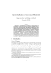
Chapter 1
Introduction
There are numerous situations where reasoning about probabilistic systems is
necessary, in fields as diverse as randomized algorithms, security, distributed systems, reliability or quantum computation.
When working with these systems, considering formal logics that capture their
probabilistic behavior is a good way to formulate properties they may or may not
satisfy. Furthermore, the development of model checking tools for formulas in such
languages over structures generated by the systems is clearly beneficial when studying the satisfaction of said properties. In [11], [14] and [15], one such logic (PCTL)
and the respective model checking tool (PRISM) are proposed. These are now
widely accepted and used in several applications. PCTL, however, only allows for
probabilistic reasoning over transitions and, in many cases, the probabilistic reasoning must be considered over states. EPPL [17] and it’s temporal extension EpCTL
[20] on the other hand, are logics that allow for quantitative probabilistic reasoning
about states and we will consider them in this thesis.
The main focus of this work is to detail the development and implementation of
a Model Checker for EPPL over digital circuits. Traditional digital circuits model
checking tools assume that each logical gate in a circuit is completely reliable, deterministically providing an output for a given input. This is an increasingly unrealistic
assumption; as hardware circuits become more and more miniaturized they also become more sensitive to noise from outside sources, either macrophysical or, in more
recent years, microphysical. Due to it’s stochastic nature, EPPL proves ideal to
model these circuits.
Besides the model checking algorithm itself, we present several relevant results
concerning both the state logic and it’s temporal extension. This work is very well
covered in [19] and, therefore, we will provide only the general guidelines. We derive a small model theorem for EPPL which allows us to propose a PSPACE SAT
algorithm for the state logic. This SAT algorithm is then used to obtain a weakly
1
2
CHAPTER 1. INTRODUCTION
complete Hilbert calculus for EPPL. One such calculus is also obtained for the temporal extension EpCTL and a general model checker for this logic is proposed.
The presentation is structured as follows. In Chapter 2, we present the state
logic, EPPL. Syntax and semantics are introduced. Afterwards, the small model
theorem is derived and the SAT algorithm described. We finish the chapter presenting the complete Hilbert calculus for EPPL.
In Chapter 3 we explain the implementation of the model checking algorithm
for EPPL for digital circuits. We start by setting notation and implementation constraints. We then describe a structure that accurately models faulty digital circuits
and how it relates to EPPL. A presentation of the algorithm follows, along with a
proof of its soundness and completeness. An informal complexity analysis is also
provided. Since efficiency concerns are taken into account, several optimization options are then discussed and their soundness is explained.
In Chapter 4, we introduce the temporal extension EpCTL much in the same
way we did with EPPL in Chapter 2: We start by defining the syntax and semantics
of the logic, then proceed to present a complete Hilbert calculus for it. Finally, we
present the general model checking algorithm for EpCTL and discuss integration of
the MC for EPPL from the previous chapter in this extended algorithm.
Finally, in the Conclusion we assess our work and what remains to be done, as
well as presenting some questions for further research.
Main contributions
The contributions of the thesis are twofold:
• Model checking noisy digital circuits: we improved the EPPL model-checking
algorithm from EXPSPACE in the number of propositional symbols to PSPACE
by taking advantage of realistic independence assumptions used when building
the circuits.
• A tool that implements the previous algorithm, that is, a model checker that
receives as input an EPPL formula and an unreliable digital circuit and outputs
1 if the formula is satisfied by the circuit and 0 otherwise.
Chapter 2
State Logic - EPPL
A probabilistic logic is necessary in order to reason about probabilistic states.
We will consider for this purpose the Exogenous Probabilistic Propositional Logic
(EPPL) [17]. In this chapter, a succinct description and a complete Hilbert calculus
for EPPL is presented, as basic knowledge of the logic is required for the following
chapters. For a more complete reference on the logic, please refer to [16],[17], [19],
[18].
2.1
Syntax
The syntax of EPPL follows the exogenous approach described in [18]: We start
with a base language (propositional in this case) and define a language at an higher
level, taking base formulas as terms.
The formulas of the base language, basic formulae, are simply classical propositional formulas over a finite set of propositional symbols Λ that is our abstraction
of the program variables and states. We introduce a set of probabilistic terms that
represent real numbers to allow for quantitative reasoning.
The formulas of the second level, global formulae, allow us to perform probabilistic reasoning over basic formulae and probabilistic terms.
The syntax of the language is given by mutual recursion as presented in Table 2.1.
β := p 8 (¬β) 8 (β ⇒ β)
basic formulae
R
t := z 8 0 8 1 8 ( β) 8 (t + t) 8 (t.t)
probabilistic terms
δ := (β) 8 (t ≤ t) 8 (∼δ) 8 (δ ⊃ δ)
global formulae
where p ∈ Λ, z ∈ Z.
Table 2.1: Syntax of EPPL
Although we use the syntax in Table 2.1 for all theoretical purposes in this work,
the syntax of formulas in the tool itself differs very slightly in order to simplify the
3
4
CHAPTER 2. STATE LOGIC - EPPL
actual implementation. The deviations are dully explained in the Annexes.
Classical abbreviations for propositional connectives like disjunction (β1 ∨ β2 ),
conjunction (β1 ∧ β2 ) and equivalence (β1 ⇔ β2 ) are used freely throughout this
work for basic formulae.
Probability terms denote elements of the real numbers. We assume a finite set
of real variables, Z, ranging over elements of algebraic real numbers. Together
with the constants 0 and 1, addition and multiplication, we are able to express all
R
algebraic real numbers. Finally measure terms, terms of the form ( β), intuitively
represent the measure of the set of valuations that satisfy β.
Global formulae are either of the form (β), comparison formulas (t1 ≤ t2 ) or
built upon these by the connectives ∼, ⊃. Formulas like (β) allow us to check
if all valuations induced by the sample space satisfy β. We will use the intuitive
abbreviation (♦β) for (∼((¬β))). (♦β) is satisfied if there is at least one valuation
induced by the probability space that satisfies β but, despite the notation, it is not
a modality, since we do not have formulas such as (β).
Like we did for basic connectives, we will assume {∪, ∩, ≡} and comparison
operators {=, ≥, <, >} introduced as abbreviations in the classical way.
Notions of occurrence and substitution of terms t and global subformulas δ1 in
the global formula δ are defined as usual. For the sake of clarity, we shall often drop
parentheses in formulas and terms if it does not lead to ambiguity.
We also introduce the following sublanguage of probabilistic state formulas which
do not contain any occurrence of measure terms:
(a ≤ a) 8 (∼κ) 8 (κ ⊃ κ)
κ
:=
α
:= z 8 0 8 1 8 (α + α) 8 (α.α)
Terms of this sublanguage will be called analytical terms and formulas will be called
analytical formulas. This language is relevant because it is possible to apply the SAT
algorithm for the existential theory of the real numbers to any analytical formula.
2.2
Semantics
The models of EPPL are tuples m = (Ω, F, µ, X) where (Ω, F, µ) is a probability
space and X = (Xp )p∈Λ is a stochastic process over (Ω, F, µ) where each Xp is a
Bernoulli random variable, that is, Xp ranges over 2 = {0, 1}. Therefore, each ω ∈ Ω
induces a valuation vω over Λ such that vω (p) = Xp (ω), for all p ∈ Λ. In addition,
each basic EPPL formula β represents the measurable subset {ω ∈ Ω : β(vω ) = 1},
where β(vω ) is the denotation of β by vω .
Moreover, each basic EPPL formula β also induces a Bernoulli random variable
Xβ : Ω → 2:
• X(¬β) (ω) = 1 − Xβ (ω);
• X(β1 ⇒β2 ) (ω) = max((1 − Xβ1 (ω)), Xβ2 (ω)).
2.2. SEMANTICS
5
A simple argument of structural induction shows that {ω ∈ Ω : β(vω ) = 1} =
{ω ∈ Ω : Xβ (ω) = 1}.
Given an EPPL model m = (Ω, F, µ, X) and assignement γ for real variables,
the semantics of global formulas is defined in the following way:
• Denotation of probabilistic terms:
– [[z]]m,γ = γ(z); [[0]]m,γ = 0; [[1]]m,γ = 1;
– [[(t1 + t2 )]]m,γ = [[t1 ]]m,γ + [[t2 ]]m,γ ; [[(t1 .t2 )]]m,γ = [[t1 ]]m,γ .[[t2 ]]m,γ ;
R
– [[( β)]]m,γ = µ(Xβ−1 (1)) is the probability of observing an outcome ω
such that vω satisfies β.
• Satisfaction of global formulas:
– m, γ (β) iff Ω = Xβ−1 (1);
– m, γ (t1 ≤ t2 ) iff [[t1 ]]m,γ ≤ [[t2 ]]m,γ ;
– m, γ (∼δ) iff m, γ 6 δ;
– m, γ (δ1 ⊃ δ2 ) iff m, γ δ2 or m, γ 6 δ1 .
Closed terms are defined as terms where no real variables appear. A global
formula involving only closed terms is called a closed global formula. As the denotation of closed terms is independent of the assignement, we will drop the assignement
from the notation in such cases.
Remark 2.2.1. Let Vm = {vω : ω ∈ Ω} be the set of all valuations over Λ induced by m. Consider, for each i ∈ {0, 1}|Λ| , the set Bi = {v ∈ Vm : v(p1 ) =
i1 , . . . , v(p|Λ| ) = i|Λ| } for p1 , . . . , p|Λ| ∈ Λ and in the n − th bit of i. Let Bm be the
set of all such B. Observe that an EPPL model m = (Ω, F, µ, X) induces a probability space Pm = (Vm , Fm , µm ) over valuations, where Fm ⊆ 2Vm is the σ-algebra
generated by Bm and µm is defined over Bm by µm (B) = µ({ω ∈ Ω : vω ∈ B}) for
all B ∈ Bm . Moreover, given a probability space over valuations, P = (V, F, µ),
we can construct an EPPL model mP = (V, F, µ, X) where Xp (v) = v(p). Since
Xβ−1 (1) = {ω ∈ Ω : Xβ (ω) = 1} = {ω ∈ Ω : β(vω ) = 1}, it is easy to see that m and
mPm satisfy precisely the same formulas.
Example 2.2.2. Consider an EPPL model describing the toss of two fair coins and
checking if any of them comes up heads (=1). Each coin represents a probabilistic
bit, as does the checking action, that is, the set of propositional symbols is Λ =
{p1 , p2 , p3 }, where p1 models one coin, p2 models the other coin and p3 models the
checking action. The outcome of tossing the two coins and checking is described by
m = ({000, 011, 101, 111}, 2{001,011,101,111} , µ, X) where µ(xyz) = 41 , Xp1 (xyz) = x
and Xp2 (xyz) = y and Xp3 (xyz) = z for all x, y, z ∈ {0, 1} s.t. z = max(x, y). It is
R
easy to see that m (1 + 1 + 1 + 1)( p3 ) = (1 + 1 + 1) (which we abbreviate to
R
m ( p3 ) = 43 ).
6
CHAPTER 2. STATE LOGIC - EPPL
Example 2.2.3. Consider the more sophisticated experiment of tossing a fair
coin until the outcome is heads(=1’s). This process can be modeled by the structure m = (Ω, F, µ, X) over a countable infinite set of propositional symbols Λ =
{p1 , . . . , pn , . . .}, where
Ω = {00
. . . 0} 111 . . . : k ≥ 0}, F = 2Ω ,
| {z
k
and Xi : Ω → 2 is the state of the coin at time i ∈ N, for all pi ∈ Λ, with
1
µ(00
. . . 0} 111 . . .) = k+1
| {z
2
for k ≥ 0,
k
and zero otherwise.
m is not an EPPL model, as Λ is infinite. If we were to push the definition
and consider the same semantics, allowing infinite sets of propositional symbols, we
would have, for example, m ((pi ⇒ pi+1 )), for all i ∈ N.
Given the configuration 00
. . . 0} 111 . . . we could represent it by the basic formula
| {z
k
((¬p1 ) ∧ (¬p2 ) ∧ . . . ∧ (¬pk ) ∧ pk+1 ), but the configuration 0000 . . . could not be
represented by any basic formula, because we don’t allow infinitary conjunctions.
To avoid this limitation, we can group all variables of some index or higher
in a single variable and consider instead the model m0 = (Ω, F, µ, X0 ), over Λ =
{p1 , . . . , pn }, such that (Ω, F, µ) as above and X0 = (Xi0 : Ω → 2)1≤i≤n where Xi is
the state of the coin at time 1 ≤ i ≤ n − 1 and Xn0 is zero if the coin will never be
in state “heads” from time n and one otherwise.
In this case, the basic formula β0 = ((¬p1 ) ∧ . . . ∧ (¬pn−1 ) ∧ (¬pn )) represents
R
the configuration 0000 . . . and m0 (( β0 ) ≤ 0), but m0 6 ((¬β0 )).
Given that we are working towards a complete Hilbert calculus for EPPL through
a SAT algorithm, it is relevant to understand whether EPPL fulfills a small model
theorem. If this is the case then an upper bound on the size of the satisfying models
would imply the decidability of the logic (since it would be enough to search for
models up to this bound).
2.3
Small model theorem
The technique used in [10] to obtain a small model theorem is adapted in [19]
for EPPL.
Let δ be an EPPL formula. We denote the sets of inequalities, basic subformulas
and propositional symbols occurring in δ by iq(δ), bsf (δ) and prop(δ), respectively.
Given a formula δ and an EPPL model m = (Ω, F, µ, X), we define the following
2.3. SMALL MODEL THEOREM
7
relation on the sample space Ω:
ω1 ∼δ ω2 iff Xp (ω1 ) = Xp (ω2 ) for all p ∈ prop(δ)
Lemma 2.3.1. The relation ∼δ is a finite index equivalence relation on Ω and if
ω1 ∼δ ω2 then Xβ (ω1 ) = Xβ (ω2 ) for all β ∈ bsf (δ).
Proof. Clearly ∼δ is an equivalence relation since equality is an equivalence relation
as well. The set prop(δ) is finite, so, it allows only a finite number of different ∼δ
classes. Let ω1 , ω2 ∈ Ω such that ω1 ∼δ ω2 .
Base: true by definition.
Step:
• In the case (¬β) we have
X(¬β) (ω1 ) = 1 − Xβ (ω1 ) = 1 − Xβ (ω2 ) = X(¬β) (ω2 );
• In the case (β1 ⇒ β2 ) we have
X(β1 ⇒β2 ) (ω1 ) = max(1 − Xβ1 (ω1 ), Xβ2 (ω1 )) = max(1 − Xβ1 (ω2 ), Xβ2 (ω2 )) =
X(β1 ⇒β2 ) (ω2 ).
Let propω (δ) be the subset of propositional symbols of δ such that Xp (ω) = 1. We
denote by [ω]δ the ∼δ class of ω.
Lemma 2.3.2. Let ω ∈ Ω,

[ω]δ = 

\
{ω 0 : Xp (ω 0 ) = 1}
p∈propω (δ)

\

\

{w0 : Xp (ω 0 ) = 0} .
p∈prop(δ)\propω (δ)
Moreover, [ω]δ ∈ F.
Proof. For the first claim, observe that if ω1 ∼δ ω2 then propω1 (δ) = propω2 (δ).
Since (Xp )p∈Λ are random variables and F is closed to finite intersections we prove
the last claim.
Taking an EPPL model m = (Ω, F, µ, X) and an EPPL formula δ, we define the
quotient model m/ ∼δ = (Ω0 , F 0 , µ0 , X0 ) where:
•
Ω0 = Ω/ ∼δ
0
Ω0
is the finite set of ∼δ classes;
•
F =2
is the power set σ-algebra;
•
µ0 (B) = µ(∪B)
for all B ∈ F 0 ;
•
Xp0 ([ω]δ ) = Xp (ω)
for all p ∈ Λ.
8
CHAPTER 2. STATE LOGIC - EPPL
The quotient model is well defined.
Proposition 2.3.3. Let m = (Ω, F, µ, X) be an EPPL model and δ an EPPL
formula, then m/ ∼δ = (Ω0 , F 0 , µ0 , X0 ) is a finite EPPL model .
Proof. By Lemma 2.3.1, Ω0 is a finite set. If B ∈ F 0 , then ∪B = ∪{[s]δ : [s]δ ∈ B}
is in F by Lemma 2.3.2. By definition we get that µ0 ([s]δ ) = µ([s]δ ) and µ0 (Ω0 ) =
µ(∪Ω0 ) = µ(Ω) = 1. So, µ0 is a finite probabilistic measure over Ω0 .
If we prove that satisfaction is preserved by the quotient construction, then any satisfiable formula ξ has a finite discrete EPPL model of size bounded by the formula
length |ξ|.
Theorem 2.3.4 (Small Model Theorem). If δ is a satisfiable EPPL formula then
it has a finite model using at most 2|δ| + 1 algebraic real numbers.
Proof. Let m = (Ω, F, µ, X) be an EPPL model of δ and m0 = m/ ∼δ its quotient
model, that is, a finite discrete EPPL model of size 2|prop(δ)| ∈ O(2|δ| ).
In the quotient model m0 , we need a real number for each valuation over prop(δ),
therefore we need at most 2|δ| real numbers. We start by proving that m0 satisfies
δ. Note that m and m0 agree in the denotation of probabilistic terms. The only
R
non-trivial case are the terms ( β). For β ∈ bsf (δ) and using Lemma 2.3.2 we get
R
R
[[ β]]m0 ,γ = µ0 (Xβ0 = 1) = µ(∪{Xβ0 = 1}) = µ(Xβ = 1) = [[ β]]m,γ ,
for any assignement γ of the real variables. By structural induction on terms of δ
we get that m and m0 agree on inequations.
For any subformula β of δ we have that m, γ β iff Ω = Xβ−1 (1) iff Ω0 =
0 −1
(Xβ ) (1) iff m0 , γ β. Now, since m and m0 agree on inequations (t1 ≤ t2 ) and
modal formulas β, we get by structural induction that m0 is a model for δ.
00
Finally, we will simplify m0 to obtain a model m00 = (Ω00 , 2Ω , µ00 , X00 ) of δ such
−1
that |Ω00 | ≤ 2|δ| + 1. Let bsf (δ) = {β1 , . . . , βk } and Ω0βi = X 0 βi (1) ⊆ Ω0 . Observe
that k ≤ |δ|. Then, we can build a system of k+1 equations
 P
0


ω∈Ω0β xω = µ (Xβ1 = 1)

1


 ...
P
0


ω∈Ω0β xω = µ (Xβk = 1)

k


 P
ω∈Ω0 xω = 1
for which we know that there is a non-negative solution xω = µ0 ({ω}) for all ω ∈ Ω0 .
From linear programming it is well known that if a system of k + 1 linear equations
has a non-negative solution, then there is a solution ρ for the system with at most
k + 1 variables taking positive values [4]. Then, we can construct a model m000
such that Ω000 = {ω ∈ Ω0 : ρ(xω ) > 0} and µ000 ({ω}) = ρ(xω ). Observe that
2.4. DECISION ALGORITHM FOR EPPL SATISFACTION
9
m000 (t1 ≤ t2 ) iff m0 (t1 ≤ t2 ) for each inequation (t1 ≤ t2 ) occurring in δ.
However, it might be the case that m000 β and m0 6 β for some subformula
β of δ, since Ω000 ⊆ Ω0 . Then, for each subformula β of δ such that m0 6 β and
m000 β there exists ωβ ∈ Ω0 \ Ω000 such that vωβ 6 β. We can now construct the
model m00 where
Ω00 = Ω000 ∪ {ωβ ∈ Ω0 \ Ω000 : m0 6 β and m000 β},
(
µ00 (ω) =
µ000 (ω)
if ω ∈ Ω000
0
otherwise
and Xp00 (ω) = Xp0 (ω) for all ω ∈ Ω00 . Clearly, |Ω00 | ≤ 2|δ| + 1 and m00 δ. Finally,
from the first order theory of real ordered fields, if there is a model using real
numbers for a real closed formula, then there is a model using only algebraic real
numbers [1] (since the logic cannot specify transcendental real numbers with a
single formula – we need an infinite number of formulas to be able to specify a
transcendental real number), so the solution of the system can be made just with
algebraic real numbers.
The size of the representation of the algebraic real numbers can increase without
any bound. Fortunately, thanks to the fact that the existential theory of the real
numbers can be decided in PSPACE, we find a bound on the size of the real representations in function of the size of the formula, which will lead to a SAT algorithm
for EPPL.
2.4
Decision algorithm for EPPL satisfaction
Given an EPPL formula δ we will denote by iq(δ) the set of all subformulas of
δ of the form (t1 ≤ t2 ), by bf (δ) the set of all subformulas of δ of the form β
and at(δ) = bf (δ) ∪ iq(δ). By an exhaustive conjunction ε of literals of at(δ) we
mean that ε is of the form α1 ∩ · · · ∩ αk where each αi is either a global atom or a
negation of a global atom. Moreover, all global atoms or their negation occur in ε,
so, k = |at(δ)|. Given a global formula δ, we denote by δpαα the propositional formula
obtained by replacing in δ each global atom α with a fresh propositional symbol
pα , and replacing the global connectives ∼ and ⊃ by the propositional connectives
¬ and ⇒, respectively. We denote by vε the valuation over propositional symbols
pα such that v (pα ) = 1 iff α occurs not negated in ε.
Given an exhaustive conjunction ε of literals of at(δ), we denote by lbf (ε) the
set of basic formulas such that β ∈ lbf (ε) if β occurs positively in ε (that is,
not negated). Similarly, the set of basic formulas that occur nested by a ∼ in ε is
denoted by lbf♦¬ (ε). Finally, we denote all the inequality
literals occurring in ε by
R
( β)
liq(ε). Given a global formula α in liq(ε) we denote by αP{xv :v∈V,vβ} the analytical
R
P
formula where all terms of the form ( β) are replaced in α by v∈V,vβ xv where
10
CHAPTER 2. STATE LOGIC - EPPL
each xv is a fresh variable. We need a PSPACE SAT algorithm of the existential
theory of the reals numbers, that we denote by SatReal. We assume that this
algorithm either returns no model, if there is no solution for the input system of
inequations, or a solution array ρ, where ρ(x) is the solution for variable x. We
denote by var(δ) the set of real logical variables that occur in δ. Given a solution ρ
for a system with X variables and a subset Y ⊆ X, we denote by ρ|Y the function
that maps each element y of Y to ρ(y).
Algorithm 1: SatEPPL(δ)
Input: EPPL formula δ
Output: (V, µ) (denoting the EPPL model m = (V, 2V , µ, X)) and
assignement γ or no model
compute bf (δ), iq(δ) and at(δ);
foreach exhaustive conjunction ε of literals of at(δ) such that vε δpαα do
compute lbf (ε), lbf♦¬ (ε) and liq(ε);
foreach V ⊆ 2prop(δ) such that 0 < |V | ≤ 2|δ| + 1, V ∧lbf (ε) and
V 6 β for all β ∈ lbf♦¬ (ε)
doT
P
κ ←−
x
=
1
∩
v∈V v
v∈V 0 ≤ xv ;
foreach α ∈ liq(ε)
do
R
( β)
κ ←− κ ∩ αP{xv :v∈V,vβ};
end
ρ ←− SatReal(κ);
if ρ 6= no model then
µρ ←− ρ|{xv :v∈V } ;
γρ ←− ρ|var(δ) ;
return (V, µρ ) and assignement γρ ;
end
end
end
return (no model);
We claim that Algorithm 1 decides the satisfiability of an EPPL formula in
PSPACE and to support this claim, we explain the algorithm and its soundness:
Given an EPPL formula δ, we start by computing (line 1) its global atoms
bf (δ), iq(δ) and at(δ). This sets take O(|δ|) space to store.
Now, we cycle over all exhaustive conjunctions ε such that vε δpαα . Observe
that if δ has a model m, γ then, for all δ 0 ∈ at(δ) this model is such that either
m, γ δ 0 or m, γ 6 δ 0 . Therefore, there is an exhaustive conjunction ε such that
m, γ is a model of ε and, in this case, vε δpαα . On the other hand, if δ has no
model, then all ε such vε δpαα have no model. Hence, to find a model for δ it is
enough to find a model for an ε such that vε δpαα . At each step of the cycle of the
second line of the algorithm, we only need to store one such ε, which requires only
2.5. COMPLETENESS OF EPPL
11
polynomial space.
To check if there is an EPPL model for ε we start by computing lbf (ε), lbf♦¬ (ε)
and liq(ε), which can be stored in O(|ε|). Given Remark 2.2.1, it is enough to check
for models where the state space Ω is given as a set of valuations of the basic propositional symbols. Moreover, thanks to the small model theorem (Theorem 2.3.4),
it is enough to search for sets of valuations V such that |V | ≤ 2|δ| + 1. V has to
satisfy the modal literals β and ∼β occurring in ε, that is: for all β ∈ lbf (ε)
and v ∈ V we have that v β, which can be written as V ∧lbf (ε) and for all
β ∈ lbf♦∼ (ε) there exists v ∈ V such that v 6 β wich can be written as V 6 β
for all β ∈ lbf♦¬ (ε). These are exactly the conditions in the guard of the second
cycle of the program. In the body of this cycle we will check if there is a model of ε
taking such V as the set of states, that is, if there is a solution for the inequations
in liq(). Since we only have to store a set of valuations V with |V | ≤ 2|δ| + 1 at
each step of the cycle, once again we need only polynomial space.
Next, we search for a model of the inequations in liq(ε) having a set of states V .
To this end we consider a fresh real logical variable xv for each v ∈ V representing
its probability. The idea behind this step is to build an analytical formula κ that
specifies the two probability constrains expressed in the fifth line and the inequations
R
in liq(ε). Two lines further, the formula κ is finished by replacing the terms ( β) in
P
liq(ε) by v∈V :vβ xv . In line 9 we call the SatReal algorithm for a solution (model)
to κ. Since |κ| is polynomial on |δ| and the set of variables in κ is polynomially
bounded by |δ|, the SatReal will compute the solution in PSPACE. If such solution
ρ exists, we have succeeded in finding a model for δ. Hence, we return (V, µρ )
and γρ , where µρ (v) is ρ(xv ) and γρ is the restriction of ρ to var(δ). As stated in
Remark 2.2.1, this is enough to construct an EPPL model. If there is no solution
ρ then we cannot find a solution for the set V of valuations, and have to try with
another V . Finally, if for all ε and V we are not able to find a solution, then there
is no model for δ.
2.5
Completeness of EPPL
It is shown in [18] that EPPL is not compact, therefore, it is impossible to obtain
a strongly complete axiomatization for EPPL . Nevertheless, weak completeness is
enough for verification purposes, since a program specification generates a finite
number of hypothesis. The EPPL SAT algorithm allows us to show that the calculus presented in Table 2.2 is weakly complete.
The soundness of the calculus of Table 2.2 is straightforward, and so, we focus
on the completeness result.
Theorem 2.5.1. The set of rules and axioms of Table 2.2 is a weakly complete
axiomatization of EPPL.
12
CHAPTER 2. STATE LOGIC - EPPL
Table 2.2: Complete Hilbert calculus for EPPL
Axioms:
• [CTaut] `EPPL (β) for each valid propositional formula β;
• [GTaut] `EPPL δ for each instantiation of a propositional tautology δ;
• [Lift ⇒] `EPPL ((β1 ⇒ β2 ) ⊃ (β1 ⊃ β2 ));
• [Eqv ⊥] `EPPL (⊥⇔ ⊥
⊥);
• [RCF] `EPPL (t1 ≤ t2 ) for each instantiation of a valid analytical inequality;
R
• [Prob] `EPPL (( >) = 1);
R
R
R
R
• [FAdd] `EPPL ((( (β1 ∧ β2 )) = 0) ⊃ (( (β1 ∨ β2 )) = ( β1 ) + ( β2 )));
R
R
• [Mon] `EPPL ((β1 ⇒ β2 ) ⊃ (( β1 ) ≤ ( β2 )));
Inference Rules:
• [Mod] δ1 , (δ1 ⊃ δ2 ) `EPPL δ2 .
Proof. As is common in completeness results, we use a contrapositive argument: if
6` δ then 6 δ. A formula δ is said to be consistent if 6` ∼δ. So, if we prove that
every consistent formula δ has a model we get the completeness result. Observe
that if 6` δ then 6` ∼∼δ, that is, ∼δ is consistent. Therefore, if we can prove it has
a model, 6 δ.
So, we will prove that every consistent formula δ has a model. Assume by
contradiction that δ is consistent and the SAT algorithm returns no model. Let
A = {ε exhaustive conjunction of literals : vε δpαα }. By the completeness of
α
propositional logic it follows that ` (∨ε∈A εα
pα ) ⇔ δpα , and by GTaut we have
` ∪A ≡ δ. If δ is consistent then there is ε consistent, and if δ has no model, then
the consistent ε has no model as well. If the SAT algorithm returns no model for ε
it must be because of one of the following two causes: (i) it cannot find a V at the
second foreach; (ii) for all viable V the SatReal algorithm returns no model. We
will now show that for both cases we can contradict the consistency of ε.
In case (i) – no V can be found at the second foreach – it cannot be because
|V | > 2|δ|+1, thanks to the small model theorem. This means that if we remove the
bound 0 < |V | ≤ 2|δ| + 1, and consider all possible sets of valuations the algorithm
would also fail. In particular, take V = 2prop(δ) , it must happen (a) V 6 ∧lbf (ε)
or (b) V β for some β ∈ lbf♦¬ (ε). For case (a) we have that 6 ∧lbf (ε) and so,
6 β for some β ∈ lbf (ε), or equivalently β ⇒ ⊥. But by completeness of the
propositional calculus we have that ` β ⇒ ⊥, by CTaut we have that ` (β ⇒ ⊥)
and by Lift⇒ and Eqv⊥ we have that ` ∼(β) from which follows ` ∼ε which
contradicts the consistency of ε. In case (b) there is β ∈ lbf♦¬ (ε) such that β is a
tautology. Then, by CTaut, ` β. From the last derivation we get ` ∼ε, which
contradicts the consistency of ε.
In case (ii), the algorithm returns no model for all viable V computed in the
2.5. COMPLETENESS OF EPPL
13
second foreach. Thanks to the small model theorem it means that the algorithm
would also return no model for all V such that
V ∧lbf (ε) and V 6 β for all β ∈ lbf♦¬ (ε),
(2.1)
independently of the bound on the size of V . The sets of valuations satisfying (2.1)
are closed for unions, and therefore there is the largest V fulfilling (2.1), say Vmax ,
and for this set the algorithm would return no model. Let V c = 2prop(δ) \ Vmax ,
since ε is consistent it is easy to see that ε0 = ε ∩ ((∩v∈V c ¬βv )) is consistent,
where βv is a propositional formula that is satisfied only by valuation v. Therefore,
` ε0 ⊃ ε. Moreover, ` ∧lbf (ε) ⇒ ¬βv for all v ∈ V c , from which we derive that
` (∩β∈lbf (ε) β) ⊃ (∩v∈V c ¬βv )
and so ` ε ⊃ ε0 and therefore ` ε0 ≡ ε. Thus, if ε is consistent then ε0 is also
consistent, and if there is no model for ε then there is no model for ε0 as well, and
the algorithm will fail precisely in line where it returns a model.
By RCF we have ` ∼κx(Rv βv ) , where κx(Rv βv ) is the formula κ where we replace
R
each variable xv by the term βv with βv a propositional formula that is satisfied
R
only by v. By Prob, FAdd and Mon we have ` (¬βv ) ⊃ (( βv ) = 0), thus we
can derive
R
` ε0 ⊃ (∩v∈V c (( βv ) = 0)).
(2.2)
From ` ∼κx(Rv βv ) and FAdd and RCF we obtain that
R
` ∩v∈V c (( βv ) = 0) ⊃ ∼ ∩α∈liq(δ) α.
(2.3)
Finally, by CTaut we have
` ∼ ∩α∈liq(δ) α ⊃ ∼ε0 .
(2.4)
So, from (2.2), (2.3) and (2.4) we obtain with tautological reasoning ` ε0 ⊃ ∼ε0
from which we conclude ` ∼ε0 . This contradicts the consistency of ε0 and thus, the
consistency of δ. For this reason there must be a model for ε0 and consequently, a
model for δ.
14
CHAPTER 2. STATE LOGIC - EPPL
Chapter 3
Verifying Digital Circuits
with EPPL
In this section, we discuss a model checker for EPPL with applications to simple
unreliable digital circuits. Its actual implementation in the C programming language is presented in the appendix. To model unreliable digital circuits we devise
and propose the concept of probabilistic Boolean circuits (PBC). A PBC is able to
model any digital circuit with faulty logical gates, that is gates that are prone to an
error with a certain known probability, which is reasonable, since actual hardware
components explicitly state their reliability. We will show how EPPL can be used
to achieve this goal.
3.1
Notation and conventions
At this point, it is convenient to make a disambiguation: for the rest of this chapter, the word “Model” (capitalized) will be used to denote EPPL models, whereas
the word “model” (not capitalized) will be used without this connotation.
It has already been seen that each ω ∈ Ω induces a valuation vω over Λ. In this
chapter, this association will be injective, which amounts to saying that the sample
space Ω is finite and for each valuation v ∈ 2Λ , there is at most one ωv ∈ Ω. This
is a reasonable assumption because one only works with variables of the stochastic
process X or continuous functions of these variables and is, therefore, unable to
distinguish between different elements of Ω that induce the same valuation. Furthermore, as already observed in Remark 2.2.1, given any Model, there is always a
Model over valuations that satisfies the same formulas. Due to this identification,
the elements of the sample space will be abusively referred to as valuations. We will
also assume that there are no valuations in Ω with zero measure, so it is possible
that some valuations are not represented in Ω.
Under these assumptions, knowledge of the joint distribution of the random variables Xpi is enough to describe an EPPL Model. Given P(Xp1 ,...,Xpn ) (Xp1 , ...Xpn ),
15
16
CHAPTER 3. VERIFYING DIGITAL CIRCUITS WITH EPPL
• Ω = {x ∈ 2Λ : P (Xp1 = x1 , ..., Xpn = xn ) > 0},
• F = 2Ω ,
• µ({ω}) = P (Xp1 = ω1 , ..., Xpn = ωn ), Ω being finite, it is enough to define µ
for each singleton set {ω} ⊂ Ω.
Since we have to deal with computer representation, probabilities will be represented by floating points and not symbolically by algebraic real numbers. This
is not a major theoretical problem, as floating point numbers represent rational
numbers, which are algebraic numbers; however, issues of lack of precision for using floating point representation cannot be easily avoided. In this work we do not
preform an error analysis due to floating points (which is also the case for other
model-checkers, like PRISM). However, we do try to minimize the number of operations that manipulate probabilities in order to slow the propagation of these
errors.
3.2
Probabilistic Boolean circuits
Boolean circuits are the standard choice to model digital circuits. However, they
lack structure to account for error in logical gates, which happens in practice. The
following definition builds upon the concept of Boolean circuit, allowing a probabilistic error:
Definition 3.2.1. A probabilistic Boolean circuit (PBC ) is a directed acyclic graph
where each vertex i is labeled with a Bernoulli random variable Ri with expected
value ri , a fresh Boolean variable xi and a Boolean function gi : {0, 1}k+1 → {0, 1}
with domain in the variables labeling vertices pointing to i.
A vertex whose indegree is zero is called an input vertex, and its labeling variable
is called an input variable. A vertex whose outdegree is zero is called an output
vertex, and its labeling variable is called an output variable. A vertex that is neither
an input vertex nor an output vertex is called an internal vertex. If there is an arrow
pointing from vertex i to vertex j, j is said to be a child of i, and i is said to be a
parent of j. The set of parent vertices of a vertex i is denoted by par(i).
Each non-input vertex i represents a logical gate that computes the Boolean
function expressed by the formula fi . This computation returns the correct output
with probability ri . The variable xi does the double duty of identifying the vertex
and representing the outcome of this (probabilistic) computation.
For implementation purposes, we notice that in order to specify a vertex, we
only need the associated expected value ri (that we will represent with a floating
point between 0 and 1), the variable xi and the Boolean function fi (that we will
3.2. PROBABILISTIC BOOLEAN CIRCUITS
17
Figure 3.1: Sample gate
represent by a formula in the obvious way). We will henceforth adopt these syntactic
representations of PBCs, which we shall call Specifications of probabilistic Boolean
circuit (SPBC).
An arrow of a PBC or SPBC represents the dependency relation between the
head (where the arrow points to) and the tail (where the arrow comes from): one
needs the values of the propositional symbols in order to compute the value of the
labeling function.
We will make use of graphical representations of SPBCs borrowing from standard
notation of Boolean circuits and extending upon it: each vertex will be represented
by a box either labeled with the function fi or with a characteristic shape for widely
used connectives. The expected value of the Bernoulli random variable Ri will be
written under the box and it’s labeling variable, representing the output of the
probabilistic computation will be, as usual, placed after the box. The lines entering
from the left of the box represent the outputs of other gates that are to be used
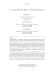
as inputs. Consider, as an example, Figure 3.1: It represents a gate that computes
f3 (x1 , x2 ) = max(x1 , x2 ) (where x1 and x2 are given as input, coming from similar
gates and f3 is represented by x1 ∨ x2 ), x3 represents the result of the probabilistic
computation that returns the value of f3 with probability 0.7 and (1−f3 ) otherwise.
SPBCs play a central role of this work because each SPBC generates an EPPL
Model where the stochastic process X is composed of random variables induced by
the vertices, their labeling functions and their labeling real numbers. Essentially,
P (Xp1 = x1 , .., Xpn = xn ) represents the probability of vertices taking the configuration hx1 , ..., xn i. Furthermore, as will be shown, these Models can be efficiently
stored and checked. We will frequently refer to vertex i of a PBC by it’s induced
random variable Xpi .
Example 3.2.2. Recall the EPPL model introduced by Example 2.2.2. It is simple
to see that the SPBC presented in Figure 3.2 induces this model. Observe that
all the relevant information is much more efficiently encoded in the PBCS than it
would be if we explicitly wrote out the probability function.
18
CHAPTER 3. VERIFYING DIGITAL CIRCUITS WITH EPPL
Figure 3.2: SPBC for double coin tossing example
3.3
Factorizations and Bayesian networks
In general, an EPPL Model representation requires an exponential space in |Λ|
(which we will denote throughout this section by n, unless stated otherwise). This
is due to the existence of Models where each pair of propositional symbols are dependent; for such Models, even the most efficient representation would have a worst
case scenario that would require writing out explicitly all of the values corresponding
to the probability attributed to each valuation, occupying O(2n ) space.
Fortunately, SPBCs are built in such a way that some degree of independence
is maintained between the variables. We will explore this property in order to get
an efficient representation of the EPPL model associated to each PBC. For this, we
will need a very simple proposition.
Lemma 3.3.1. Let X1 , ...Xn be discrete random variables. Then, for all hx1 , ..., xn i ∈
Ω,
P (X1 = x1 , ..., Xn = xn ) =
n
Y
P ∗ (Xi = xi |Xi−1 = xi−1 , ..., X1 = x1 ),
i=1
where
P ∗ (X(
i = xi |Xi−1 = xi−1 , ..., X1 = x1 ) =
=
P (Xi = xi |Xi−1 = xi−1 , ..., X1 = x1 )
if P (Xi−1 = xi−1 , ..., X1 = x1 ) 6= 0
0
otherwise
Proof. The proof is presented by induction in n.
Base: P (X1 = x1 ) = P ∗ (X1 = x1 )
Step: If P (X1 = x1 , ..., Xn−1 = xn−1 ) = 0, then P (X1 = x1 , ..., Xn = xn ) = 0
because {ω : X1 (ω) = x1 , ...Xn (ω) = xn } ⊂ {ω : X1 (ω) = x1 , ..., Xn−1 (ω) = xn−1 }.
If P (X1 = x1 , ..., Xn−1 = xn−1 ) 6= 0, then P (X1 = x1 , ..., Xn = xn ) = P ∗ (Xn =
xn |X1 = x1 , ..., Xn−1 = xn−1 )P (X1 = x1 , ..., Xn−1 = xn−1 ) by definition of con-
3.3. FACTORIZATIONS AND BAYESIAN NETWORKS
19
ditioned probability. By induction hypothesis, P (X1 = x1 , ..., Xn−1 = xn−1 ) =
Qn−1 ∗
i=1 P (Xi = xi |Xi−1 = xi−1 , ..., X1 = x1 ). Therefore, P (X1 = x1 , ..., Xn =
Qn
xn ) = i=1 P ∗ (Xi = xi |Xi−1 = xi−1 , ..., X1 = x1 ) .
We shall henceforth drop the superscript in P ∗ whenever no ambiguity arises. A
rewriting of a joint distribution function in the above form is called a factorization.
Since representing the conditional distributions P (Xpi |Xpi−1 , ..., Xp1 ) in the
worst case may take O(2i ) space, using factorizations is not, in general, an effiPn
cient way of representing EPPL models, as we could need i=1 O(2i ) = O(2n+1 )
space. However, in a SPBC, each variable induced by a vertex depends exclusively on the variables of vertices that point to it, and so P (Xpi |Xpi−1 , ..., Xp1 ) =
P (Xpi |par(Xpi )).
The structure we just described is known as a Bayesian network :
Definition 3.3.2. A Bayesian network relative to a set of random variables is a
directed acyclic graph where each vertex is labeled with one of the variables and the
joint distribution of those variables can be written as the product of the conditioned
probability of each vertex and its parents:
P (X1 , ..., Xn ) =
Qn
i=1
P (Xi |par(Xi )).
Bayesian networks have the expressive power to determine all EPPL Models
since one can always consider the Bayesian network where the parents of the vertex
labeled with Xi are all vertexes with label Xk , k < i, effectively performing a factorization. However, we have seen that, in the worst case, there are no gains in space
representation from using this approach relative to using the explicit description
of the probability distribution. Nevertheless, Bayesian networks are a well studied
object and perhaps some results from their general theory could yield interesting
consequences when studying SPBCs.
20
CHAPTER 3. VERIFYING DIGITAL CIRCUITS WITH EPPL
Fortunately, SPBCs have another property that further reduces the complex-
ity of the Model Checking algorithm: the probability of correctly computing the
Boolean functions expressed by the labeling formulas, i.e. P (Xpi = ϕi (par(Xpi )),
is known. With this information, we can prove the following result:
Theorem 3.3.3. Let (Xp1 , ..., Xpn ) be the variables induced by the vertices of a
SPBC and hx1 , ..., xn i a valuation, then:
P (Xp1 = x1 , ..., Xpn = xn ) =
n
Y
ri δxi ,ϕi + (1 − ri )δ1−xi ,ϕi
i=1
(
where ri is the real number labeling i and δxi ,ϕi =
1
if xi = ϕi (x1 , ..., xi−1 )
0
if xi 6= ϕi (x1 , ..., xi−1 )
Proof. In this proof, we denote by par(Xpi ) = par(xi ) the set {x ∈ Ω : Xpi =
xi , Xpi ∈ par(Xpi )}
In view of Lemma 3.3.1, it suffices to prove that P (Xpi = xi |Xpi−1 = xi−1 , ..., Xp1
= x1 ) = ri δxi ,ϕi + (1 − ri )δ1−xi ,ϕi .
Using the Total Probabilities theorem with the partition Ω = Ωxi =ϕi ∪ Ωxi =ϕi
where Ωxi =ϕi = {x ∈ Ω : xi = ϕi (xi−1 , .., x1 )}, we have:
P Xpi = xi |Xpi−1 = xi−1 , ..., Xp1 = x1 = P [Xpi = xi |par(Xpi ) = par(xi )] =
P [Xpi = ϕi (par(Xpi ))]×P [Xpi = xi |par(Xpi ) = par(xi ), Xpi = ϕi (par(Xpi ))] +
P [Xpi 6= ϕi (par(Xpi ))]×P [Xpi = xi |par(Xpi ) = par(xi ), Xpi 6= ϕi (par(Xpi ))] =
ri × P [xi = ϕi (par(xi ))] + (1 − ri ) × P [xi 6= ϕi (par(xi ))]
and
(
P [xi = ϕi (par(xi ))] =
(
P [xi 6= ϕi (par(xi ))] =
1
if xi = ϕi (x1 , ..., xi−1 )
0
if xi 6= ϕi (x1 , ..., xi−1 )
0
if xi = ϕi (x1 , ..., xi−1 )
i.e. (1 − xi ) 6= ϕi (x1 , ..., xi−1 )
1
if xi 6= ϕi (x1 , ..., xi−1 )
i.e. (1 − xi ) = ϕi (x1 , ..., xi−1 )
= δxi ,ϕi ,
= δ(1−xi ),ϕi ,
This Theorem provides a very simple way of computing the probability of any
given valuation, as we need only to check, for each vertex, if the denotation of the
labeling formula by the valuation yields the same value as the denotation of the
induced variable by the valuation, and return the real number labeling the vertex
or its complement, according to the result. The product of all such values will be
the desired probability.
3.4. THE BASIC ALGORITHM
3.4
21
The basic algorithm
We now describe the basic algorithm for model checking EPPL formulas in EPPL
models induced by SPBCs.
Let δ be an EPPL global formula. In the following algorithm, the arrays bf (δ) =
{λ1 , ..., λk },subR (δ) = {m1 , ..., ms }, pst(δ) = {t1 , ..., tr },gsf (δ) = {δ1 , ..., δu , δ} denote, respectively, the list of subformulas of δ of the form β, the list of measure
R
subterms of δ (of the form β), the list of probabilistic subterms of δ that are not
measure terms, the ordered tuple of basic subformulas of δ.
The symbol ω i represents the i − th valuation in 2Λ for some enumeration of
valuations over Λ.
β(ω i ) represents the algorithm that computes the denotation of β by ω i , which
is well known to take O(|βi |) time.
f act(ω i ) represents the algorithm that computes P (Xp1 = ω1i , ..., Xpn = ωni ). As
we can see from Theorem 3.3.3, this algorithm takes O(|f act|) time, where |f act| is
the size of the factorization induced by the PBC. Observe that O(|f act|) = O(n·|β|),
with |β| being the length of the largest labeling formula of the PBC and n the number of propositional connectives in Λ. One should keep in mind that whenever this
algorithm returns 0, it should be interpreted as “ω i ∈
/ Ω”, because we have no elements with measure zero in Ω.
The first part of the algorithm runs through all subformulas of the form βi
and through all valuations checking, for each valuation, both if it is in Ω and if it
does not satisfy the basic formula βi . If both answers are positive for any valuation,
there is ω ∈ Ω such that ω ∈
/ Xβ−1 (1); otherwise, Ω = Xβ−1 (1). The values of β
are stored in a Boolean |bf (δ)| array B.
Then, the algorithm runs through all subterms of the form
R
βi and through
all valuations, checking for each valuation if it is in Ω and if it satisfies the basic
formula βi . If both answers are positive, it then adds the measure of the valuation
R
to M (i), the i − th entry of the real |subR (δ)| array M , where the values of β are
stored.
The third part performs all other term evaluations, it stores them in a real
|pst(δ)| array T .
Finally, the algorithm evaluates all global subformulas to a Boolean |gsf (δ)|
array G, where G(i) = 1 iff χf act , γ δi , for all 1 ≤ i ≤ |gsf (δ)|, where χf act is the
model induced by f act and return as output G(|gsf |).
22
CHAPTER 3. VERIFYING DIGITAL CIRCUITS WITH EPPL
Algorithm 2: CheckEPPL(f act, γ, δ)
Input: Factorization f act, assignement γ and a formula δ
Output: Boolean value G(|gsf (δ)|)
for i = 1 to |bf (δ)| do
λi is β;
B(i) = 1;
for j = 1 to 2n do
If (β(ω j ) == 0 && f act(ω j ) > 0) {B(i) = 0; break; };
end
end
for j = 1 Rto |subR (δ)| do
mi is β;
M (i) = 0;
for j = 1 to 2n do
If (β(ω j ) == 1) {M (i) = M (i) + f act(ω j ); };
end
end
for i = 1 to |pst(δ)| do
switch ti do
case z : T (i) = γ(z) :;
case 0 or 1 : T (i) = ti ;
case (tj + tl ) : T (i) = T (j) + T (l);
case (tj .tl ) : T (i) = T (j).T (l);
case (mj + tl ) : T (i) = M (j) + T (l);
case (mj .tl ) : T (i) = M (j).T (l);
case (tj + ml ) : T (i) = T (j) + M (l);
case (tj .ml ) : T (i) = T (j).M (l);
end
end
for i = 1 to |gsf (δ)| do
switch δi do
case (βj ) : G(i) = B(j);
case (tj ≤ tl ) : G(i) = (T (j) ≤ T (l));
case (mj ≤ tl ) : G(i) = (M (j) ≤ T (l));
case (tj ≤ ml ) : G(i) = (T (j) ≤ M (l));
case (mj ≤ ml ) : G(i) = (M (j) ≤ M (l));
case (δj ⊃ δl ) : G(i) = max(1 − G(j), G(l));
case (∼δj ) : G(i) = 1 − G(j);
end
end
Assuming that all basic arithmetical operations take O(1) time, we see that
P
n
the first part of the algorithm takes
βi ∈bf (δ) O(2 )(O(|βi |) + O(|f act|)) =
3.4. THE BASIC ALGORITHM
O(2n )(
P
βi ∈bf (δ)
2
n
O(|βi |) +
23
P
βi ∈bf (δ)
O(|f act|)) = O(2n )O(|δ|)O(|δ| · |f act|) =
O(2 · |δ| · |f act|).
The second part takes, likewise,
PR
βi ∈subR (δ)
O(2n )(O(|βi |)+O(|f act|)) = O(2n ·
|δ|2 · |f act|).
The third cycle runs O(|δ|) times, each case being a basic operation or taking
O(|δ|) time (since both |subR (δ)| < |δ| and |pst(δ)| < |δ|). The cycle runs in O(|δ|2 ).
Finally, the last cycle runs O(|δ|) times, each case taking O(|δ|) time (since
|subR (δ)| < |δ|, |pst(δ)| < |δ| and |bf (δ)| < |δ|). The cycle runs in O(|δ|2 ).
All four rounds of the algorithm take O(2n · |δ|2 · |f act|) or less time. So the
algorithm runs in O(2n · |δ|2 · |f act|) as well.
This is slightly less time efficient than the algorithm proposed in [19]. However,
the present algorithm does not require writing out explicitly an EPPL Model, a
structure that takes exponential space in |Λ|, nor it requires at any step the use of
such large structures. In fact, none of the arrays B, M, T, G take more than O(|δ|)
space and the input itself takes O(|γ|) + O(|δ|) + O(|f act|). So, the algorithm takes
O(|γ| + |δ| + n · |β|) space, whereas the one proposed in [19] needs O(2n · |δ| + γ).
This is what we gain from using PBCs, at the cost of a little temporal efficiency.
Proposition 3.4.1. χf act , γ δ if and only if Algorithm 2 returns 1.
(
Proof. We will first prove that B(i) =
1
if χf act , γ λi
0
if χf act , γ 6 λi
:
If B(i) = 1, then, for all ω j ∈ 2Λ , either f act(ω j ) = 0 or f act(ω j ) 6= 0 and
λi (ω j ) = 1. In the first case, ω j ∈
/ Ω, and we need not consider it. In the second
case, ω j ∈ Ω and ω j ∈ Xλ−1
(1). Since we run trough all ω j ∈ 2Λ , we also exhaust
i
all ω j ∈ Ω, and each one verifies ω j ∈ Xλ−1
(1), meaning that Ω = Xλ−1
(1), i.e.,
i
i
χf act , γ λi .
If B(i) = 0, then for at least one ω j , f act(ω j ) > 0 and λi (ω j ) = 0. Since
f act(ω j ) > 0, ω j ∈ Ω, but because λi (ω j ) = 0, ω j ∈
/ Xλ−1
(1), which means there is
i
ω j ∈ ω such that ω ∈
/ Xλ−1
(1), i.e., χf act , γ 6 λi .
i
We now prove that M (i) = [[mi ]]χf act ,γ :
In the conditions of our sample space, [[mi ]]χf act ,γ = µ(Xλ−1
(1)) = µ({ω ∈ Ω :
i
P
β(ω) = 1}) = ω∈Ω:β(ω)=1 µ({ω}). Since f act(ω) = µ({ω}) if ω ∈ Ω, 0 otherwise,
M (i) =
X
f act(ω j ) =
X
f act(ω j ) +
X
f act(ω j ) =
X
µ({ω j }) +
X
ω j ∈ 2Λ :
ωj ∈ Ω :
ωj ∈
/Ω:
ωj ∈ Ω :
ωj ∈
/Ω:
βi (ω j ) = 1
βi (ω j ) = 1
βi (ω j ) = 1
βi (ω j ) = 1
βi (ω j ) = 1
X
µ({ω j }) = µ(
[
{ω j }) = µ({ω ∈ Ω : β(ω) = 1} = [[mi ]]χf act ,γ .
ωj ∈ Ω :
ωj ∈ Ω :
βi (ω j ) = 1
βi (ω j ) = 1
0=
24
CHAPTER 3. VERIFYING DIGITAL CIRCUITS WITH EPPL
It is now straightforward to check that T (i) = [[ti ]]χf act ,γ . We omit the rest of
the proof, as it is a simple but lengthy exercise of induction over |δ|.
3.5
Optimizations
The tool produced in the scope of this work is not a blind implementation of the
algorithm of the previous section: several optimizations are used in order to reduce
the time (in average) it takes to model check a formula. Unfortunately, none of
these will actually reduce the worst case complexity in which the program runs. In
this section, we will justify the major implementation deviations from the algorithm
and prove their soundness.
3.5.1
Equivalent SPBCs
Figure 3.3: Equivalent SPBCs
Example 3.5.1. Consider the SPBCs represented in Figure 3.3 . It is easy to see
that the joint distributions of (Xp1 , Xp2 , Xp3 ) and (Yp1 , Yp2 , Yp3 ) are as presented
in Table 3.1.
We have seen that, under our assumptions, knowledge of the joint distribution
is enough to fully describe the EPPL model. Since both SPBCs from Figure 3.3
induce the same distribution function, we conclude that they generate the same
EPPL model.
The previous example shows that different SPBCs can induce the same EPPL
model. Notice that PBCs corresponding to these SPBCs are not equal, yet they
3.5. OPTIMIZATIONS
25
Table 3.1: Distributions of X and Y
ω = hω1 ω2 ω3 i P (Xp1 = ω1 , Xp2 = ω2 , Xp3 = ω3 ) P (Yp1 = ω1 , Yp2 = ω2 , Yp3 = ω3 )
000
(1−0.6)×(1−0.5)×0.3 = 0.06 0.4×(1−0.5)×(1−0.7) = 0.06
001
0.14
0.14
010
0.06
0.06
011
0.14
0.14
100
0.09
0.09
101
0.21
0.21
110
0.21
0.21
111
0.09
0.09
still induce the same EPPL model. We shall say that two SPBCs induce the same
EPPL model are equivalent.
Equivalence between SPBCs is obviously an equivalence relation.
Lemma 3.5.2. Let B1 = ({Xpi }pi ∈Λ , E, {Lpi }pi ∈Λ ),B2 = ({Ypi }pi ∈Λ , E 0 , {L0pi }pi ∈Λ )
be SPBCs that have equal underlying graphs and equal labels for real numbers and
formulas in all vertices except one pair (Xpi , Ypi ), where Xi is labeled with the real
number rx and the formula ϕx and Yi is labeled with ry , ϕy .
If either (ϕx ⇔ ϕy ) (propositionally) and rx = ry or (ϕx ⇔ (¬ϕy )) and rx =
1 − ry , then B1 , B2 are equivalent.
Proof. B1 and B2 are equivalent as long as the factorizations induced by them are
equal. As all terms in the factorizations except the i − th are equal, it suffices to
prove that P (Xpi |Xpi−1 ..., Xp1 ) = P (Ypi |Ypi−1 , ..., Yp1 ) for all ω ∈ Ω.
Let ω = hω1 , ..., ωn i ∈ Ω, then
PB1 Xpi = ωi |Xpi−1 = ωi−1 , ..., Xp1 = ω1 = riB1 δωi ,ϕB1 + (1 − riB1 )δ1−ωi ,ϕB1 .
i
i
B2
1
• Case riB1 = riB2 and ϕB
i ⇔ ϕi :
B2
B1
B2
1
ϕB
i (ω1 , ..., ωi−1 ) = ϕi (ω1 , ..., ωi−1 ) because (ϕi ⇔ ϕi ).
(
δωi ,ϕB1 =
i
1
1
if ωi = ϕB
i (ω1 , ..., ωi−1 )
0
1
if ωi 6= ϕB
i (ω1 , ..., ωi−1 )
(
=
1
2
if ωi = ϕB
i (ω1 , ..., ωi−1 )
0
2
if ωi 6= ϕB
i (ω1 , ..., ωi−1 )
= δωi ,ϕB2 .
i
riB1 δωi ,ϕB1 + (1 − riB1 )δ1−ωi ,ϕB1 = riB1 δωi ,ϕB2 + (1 − riB1 )δ1−ωi ,ϕB2 =
i
i
i
i
riB2 δωi ,ϕB2 + (1 − riB2 )δ1−ωi ,ϕB2 = PB1 (Ypi = ωi |Ypi−1 = ωi−1 , ..., Yp1 = ω1 )
i
i
26
CHAPTER 3. VERIFYING DIGITAL CIRCUITS WITH EPPL
B2
1
• Case riB1 = 1 − riB2 and ϕB
i ⇔ (¬ϕi ):
B2
B1
B2
1
ϕB
i (ω1 , ..., ωi−1 ) = 1 − ϕi (ω1 , ..., ωi−1 ) because (ϕi ⇔ (¬ϕi )).
(
δωi ,ϕB1 =
i
1
1
if ωi = ϕB
i (ω1 , ..., ωi−1 )
0
1
if ωi 6= ϕB
i (ω1 , ..., ωi−1 )
(
=
0
2
if ωi = ϕB
i (ω1 , ..., ωi−1 )
1
2
if ωi 6= ϕB
i (ω1 , ..., ωi−1 )
= δ1−ωi ,ϕB2 .
i
riB1 δωi ,ϕB1 + (1 − riB1 )δ1−ωi ,ϕB1 = riB1 δ1−ωi ,ϕB2 + (1 − riB1 )δ1−(1−ωi ),ϕB2 =
i
i
i
i
(1 − riB2 )δ1−ωi ,ϕB2 + riB2 δωi ,ϕB2 = PB1 (Ypi = ωi |Ypi−1 = ωi−1 , ..., Yp1 = ω1 )
i
i
So, for each hω1 , ..., ωn i ∈ Ω, the i − th factor is also equal.
Proposition 3.5.3.
Let B1 = ({Xpi }pi ∈Λ , E, {Lpi }pi ∈Λ ), B2 = ({Ypi }pi ∈Λ , E 0 ,
{L0pi }pi ∈Λ ) be SPBCs that have equal underlying graphs and equal labels for real
numbers and formulas in all vertices except they may differ in any number of pairs
(Xpi , Ypi ), in the conditions of Lemma 3.5.2. Then B1 , B2 are equivalent.
Proof. The result follows by transitivity of the equivalence relation and Lemma
3.5.2.
Henceforth, we will assume that all SPBCs’ labeling real numbers are at least
1
2.
This can be done because we can always build a SPBC with this property that
is equivalent to any SPBC given: In any vertex of the original SPBC with labeling
number r less than 12 , we change the labeling formula ϕ to (¬ϕ) and labeling number 1 − r.
3.5.2
Deterministic gates
Suppose a SPBC where one of the vertices is labeled with the real number 1.
This amounts to saying that the connective of the digital circuit that is modeled by
that vertex is completely reliable, deterministically providing an output for given
sets of input (rigorously, providing the correct output for given sets of input with
probability one, but since the sample space is finite and does not have elements
with measure zero, we allow ourselves the language abuse).
3.5. OPTIMIZATIONS
27
We will call a vertex with this property a deterministic gate. Deterministic gates
will allow some simplifications in our algorithm, essentially removing one symbol
from Λ, for all implementation purposes. The idea is that if xi = ϕi (xi−1 , ..., x1 )
with r = 1, then we can substitute all instances of Xpi in all formulas that need to
be verified by ϕi (Xpi−1 , ..., Xp1 ).
Definition 3.5.4. Let Xpn , ..., Xp1 be discrete random variables. Xpi+1 is said to
be completely dependent of Xpi , ..., Xp1 by means of f if
µ({ω : Xpi+1 (ω) = f (Xpi (ω), ..., Xp1 (ω))}) = 1
where µ denotes the measure over the probability space underlying in the random vector Xpn , ..., Xp1 .
Proposition 3.5.5. Given SPBC B that has one deterministic gate, the random
variable Xpi induced by that vertex is completely dependent of par(Xpi ) by means
of ϕi when seen as a Boolean formula.
Proof. For all ω = hω1 , ..., ωn i ∈ Ω,
P (Xpi = ωi |Xpi−1 = ωi−1 , ..., Xp1 = ω1 ) = ri δωi ,ϕi + (1 − ri )δ1−ωi ,ϕi =
(
= δωi ,ϕi =
1
if ωi = ϕi (ω1 , ..., ωi−1 )
0
if ωi 6= ϕi (ω1 , ..., ωi−1 )
Let us suppose, by contradiction, that µ({ω : Xpi (ω) = ϕi (par(Xpi ))}) 6= 1.
Then, there is W = {ω : Xpi D
6 ϕi (par(X
=
Epi ))} such that µ(W ) > 0.
j
j
j
As W is finite, there is ω = ω1 , ..., ωn ∈ W such that µ({ω j }) > 0.
P Xpi = ωi1 |par(Xpi ) = par(ωi1 ) = δωj ,ϕj = 0 (because ω j , ωij 6= ϕ(par(ωij )))
i
i
On the other hand, as P (par(Xpi ) = par(ωij )) > 0 because ω j ∈ Ω:
h
i
h
i P Xpi = ωij , par(Xpi ) = par(ωij )
h
i
>0
P Xpi = ωij |par(Xpi ) = par(ωij ) =
P par(Xpi ) = par(ωij )
because ω j ∈ Ω. This is a contradiction.
Remark 3.5.6. At this point, it is convenient to notice that, since our sample
space is finite and has no elements with measure zero, verifying m, γ β is the
R
same as verifying if [[ β]]m,γ = 1, indeed; if m, γ β, then Ω = Xβ−1 (1), therefore
28
CHAPTER 3. VERIFYING DIGITAL CIRCUITS WITH EPPL
R
1 = µ(Ω) = µ(Xβ−1 (1)), i.e, [[ β]]m,γ = 1. On the oher hand, if m, γ 6 β,
Ω 6= Xβ−1 (1) and there is ω ∈ Ω such that ω ∈ Xβ−1 (0). Since µ(ω) > 0 and
R
Xβ−1 (1) ∩ Xβ−1 (0) = φ, [[ β]]m,γ = Xβ−1 (1) < 1.
R
In [18], β is actually introduced as an abbreviation of β = 1, but slight differences in semantics do not allow us to take this shortcut in this work.
Finally, we can claim the following result:
Proposition 3.5.7. Let Xpi+1 be completely dependent of Xpi , ..., Xp1 by means
of f , m be an EPPL model induced by a SPBC, γ an assignement and δ a global
formula. Then
p
m, γ δ iff m, γ δf i+1
(pi ,...,p1 )
Proof. Notice that all nonbasic subformulas of δ remain unchanged by the substiR
R p
tution. Therefore, if we prove both that [[ β]]m,γ = [[ βf i+1
(pi ,...,p1 ) ]]m,γ and that
p
m, γ β iif m, γ βf i+1
(pi ,...,p1 ) , the result will follow.
R
R p
In view of Remark 3.5.6, we need only prove that [[ β]]m,γ = [[ βf i+1
(pi ,...,p1 ) ]]m,γ .
R
[[ β]]m,γ = µ(Xβ−1 (1)) = µ({ω ∈ Ω : Xβ (ω) = 1})
R p
−1
[[ βf i+1
(1)) = µ({ω ∈ Ω : Xβ pi+1
(ω) = 1})
(pi ,...,p1 ) ]]m,γ = µ(X pi+1
βf (p
f (pi ,...,p1 )
i ,...,p1 )
We show that {ω ∈ Ω : Xβ (ω) = 1} = {ω ∈ Ω : Xβ pi+1
(ω) = 1}:
f (pi ,...,p1 )
Since µ({ω : Xi+1 (ω) = f (Xi (ω), ..., X1 (ω))}) = 1 = µ(Ω) and Ω is finite and
has no elements with measure zero, by elementary measure theory, {ω : Xi+1 (ω) =
f (Xi (ω), ..., X1 (ω))} = Ω.
Let ω 0 ∈ {ω ∈ Ω : Xβ (ω) = 1}. As ω 0 ∈ Ω, Xpi+1 (ω 0 ) = f (Xpi (ω 0 ), ..., Xp1 (ω 0 )).
Then, it must be the case that Xβ pi+1
(ω 0 ) = 1, as all functions in the re-
f (pi ,...,p1 )
cursive definition of Xβ pi+1
f (pi ,...,p1 )
are evaluated in the same way as in Xβ , and
f (Xpi (ω 0 ), ..., Xp1 (ω 0 )) agrees with Xpi+1 (ω 0 ).
Therefore, ω 0 ∈ {ω ∈ Ω : Xβ pi+1
0
(ω) = 1}.
f (pi ,...,p1 )
On the other hand, let ω ∈ {ω ∈ Ω : Xβ pi+1
(ω) = 1}. By the same
f (pi ,...,p1 )
0
reasoning, mutatis mutandis, we conclude that ω ∈ {ω ∈ Ω : Xβ (ω) = 1}.
This proposition allows the following simplification in the algorithm: by replacing all variables induced by deterministic gates with the function induced by the
corresponding formula, the number of valuations that have to be considered halves
for each deterministic gate, as one of each of the two valuations that only differ in
the deterministic variable would have measure zero, and, therefore, doesn’t need to
be considered.
Remark 3.5.6 shows that, given the particular structure of our sample space,
R
we may consider subformulas of the form β as β = 1. We refrain from doing
3.5. OPTIMIZATIONS
29
so in our implementation for efficiency reasons: As we can see from the basic algorithm, we always have to run exhaustively trough all 2n valuations in 2Λ in order to
R
compute [[ β]]χf act ,γ , whereas to compute χf act , γ β, the computation ends as
soon as we find a suitable valuation. The process of computing χf act , γ β can
be further refined using deterministic gates, and the program explores this property:
Theorem 3.5.8. Given a basic formula β and a SPBC induced EPPL Model χf act ,
then χf act , γ 6 β iff (¬βϕpii∈D
(pi−1 ,...,p1 ) ) is satisfiable as a propositional formula,
where D denotes the set of deterministic gates in the SPBC.
0
(Λ\D)
Proof. If (¬βϕpii∈D
s.t.
(pi−1 ,...,p1 ) ) is satisfiable, there is a valuation ω ∈ 2
0
Λ
0
(¬βϕpii∈D
(pi−1 ,...,p1 ) )(ω ) = 1. Let ω ∈ 2 be the valuation that coincides with ω in
all pi ∈ Λ \ D and that has ωi = ϕi (ωi−1 , ..., ω1 ) for all pi ∈ D (this computation
should be made by index order).
Qi=1
Q
f act(ω) = n ri δωi ,ϕi + (1 − ri )δ1−ωi ,ϕi = pi ∈D ri δωi ,ϕi + (1 − ri )δ1−ωi ,ϕi ∗
Q
Q
Q
pi ∈Λ\D ri δωi ,ϕi +(1−ri )δ1−ωi ,ϕi =
pi ∈D (1+0)∗ pi ∈Λ\D ri δωi ,ϕi +(1−ri )δ1−ωi ,ϕi
Q
= pi ∈Λ\D ri δωi ,ϕi +(1−ri )δ1−ωi ,ϕi . Each ri and 1−ri in the last product is greater
than zero, and one of the δ in each term is 1. It follows that f act(ω) > 0, that is,
ω ∈ Ω.
(¬β)(ω) = 1, as we have seen in the proof of Proposition 3.5.7.
Since µ(ω) > 0, ω ∈ Ω, then χf act , γ 6 β iff there is ω ∈ Ω s.t. ω ∈ Xβ−1 (0),
−1
i.e., there is ω ∈ Ω s.t. ω ∈ X(¬β)
(1), i.e. there is ω ∈ Ω s.t. (¬β)(ω) = 1, which we
have just proved.
0
(Λ\D)
If (¬βϕpii∈D
we have that
(pi−1 ,...,p1 ) ) is not satisfiable, for all valuations ω ∈ 2
0
βϕpii∈D
(pi−1 ,...,p1 ) (ω ) = 1.
For each ω 0 ∈ 2(Λ\D) only the ω ∈ 2Λ built in the same way as in the first part
of the proof verifies f act(ω) > 0 (i.e., ω ∈ Ω): if ωi 6= ϕi (ωi−1 , ..., ω1 ) for some pi ∈
Λ\D, the corresponding term in f act(ω), ri δωi ,ϕi +(1−ri )δ1−ωi ,ϕi = 1∗0+0∗1 = 0,
and f act(ω) = 0. Furthermore, there are no more valuations in Ω than those of this
0
form or there would be ω 0 ∈ 2(Λ\D) s.t. βϕpii∈D
(pi−1 ,...,p1 ) (ω ) = 0.
Once again, by proposition 3.5.7, β(ω) = 1. This is true for all ω ∈ Ω, and so
χf act , γ β
The previous proposition allows us to compute χf act , γ β with a single
application of a SAT algorithm for propositional logic. Although still in the same
complexity class of the direct computation of χf act , γ β, the SAT problem is
very well studied, and many clever algorithms have been proposed to solve it. Upon
the use of one such algorithm, we improve our own, since our approach in the basic
algorithm was to run through all of the 2n valuations.
30
CHAPTER 3. VERIFYING DIGITAL CIRCUITS WITH EPPL
3.6
3.6.1
EPPL MC tool
Syntax differences
Although operational aspects of the actual implementation of the tool are left
for the Appendix, there are differences between the syntax of EPPL and that of the
actual tool that we will discuss at this point.
In practice, the tool parses strings inputed by the user and, since ASCII encoding does not allow the representation of all EPPL symbols, we need to find
intuitive substitutes. There are also slight differences in parenthesis that ease the
implementation of the parsing tool.
We start by defining the syntax for basic formulas:
β := var 8 (˜β) 8 (β& β) 8 (β | β) 8 (β => β) 8 (β <=> β)
Since the parser is quite strict, when using the tool, we advise not to deviate from
the above syntax. This includes droping parenthesis or assuming associativity. One
should pay close attention to spacing: there is a whitespace after each connective.
The syntax should be clear: var stands for any variable name, ˜ stands for ¬,
& stands for ∧, | stands for ∨, => stands for ⇒ and <=> stands for ⇔. Variable
naming is duly covered in the Appendix.
For terms, the syntax is as follows:
t := {term} 8 {0} 8 {1} 8 {$β} 8 {t+ t} 8 {t. t}
The syntax is straightforward; the only connective that needs explaining is $,
R
which stands for . Remember the variable naming conventions for term variables.
The seemingly redundant {} around the variables and constants are necessary in
order to contextualize the parser.
Finally, for global formulas, the syntax is:
δ := [#β] 8 [t < t] 8 [t > t] 8 [t t] 8 [t t] 8 [t= t] 8
[!δ] 8 [δ&& δ] 8 [δ || δ] 8 [δ ==> δ] 8 [δ <==> δ]
Once again, the peculiar parenthesis are necessary to contextualize the parser.
As for connectives, <, > and = stand for themselves, # stands for ,
,
stand
for ≤, ≥ and !, &&, ||, ==>, <==> stand for ∼, ∩, ∪, ⊃, ≡, respectively.
Take, for example, axiom FAdd from Table 2.2. For this tool’s purposes, it
should be written as:
[[{$(β1 & β2 )} = {0}] ⊃ [{$(β1 ∨ β2 )} = {{$β1 } + {$β2 }}]]
As for SPBCs, the file with the description should contain one line for each
vertex. The line starts with the name of a fresh labeling variable (that will be
3.6. EPPL MC TOOL
31
identified with the induced random variable), followed by an “=”, a whitespace,
then comes the labeling basic formula (with syntax as above), followed by another
whitespace and, finally, the labeling float.
The SPBC file from Example 2.2.2, for instance, would be:
Xp1 = 1 0.5
Xp2 = 1 0.5
Xp3 = (Xp1 | Xp2 ) 1
3.6.2
A simple case study
We now introduce, as an example of application of the MC tool, a simple hypothetical case study on reliability and quality control.
Gates that compute usual Boolean functions (like conjunction or disjunction of
multiple inputs) are massively produced due to their many applications. However,
gates for more unusual functions are often required. In such cases, one of the
approaches used is to build a circuit that computes the function and have the whole
circuit acting as a single gate. This is usually done automatically, through the
function’s minterm form1 (also known as sum-of-terms form).
To build a minterm representation, one takes all configurations of inputs that
yield result 1 and, for each of them, considers the product of all variables that take
value 1 in that configuration and 1 minus the variables that take value 0 in that
configuration. The minterm representation is the sum of all such products.
Example 3.6.1. Consider the Boolean function represented in table 3.2. Since
only the configurations h0, 0, 1i , h0, 1, 0i and h1, 0, 0i yield the result 1, its minterm
form is
f (x, y, z) = (1 − x)(1 − y)z + (1 − x)y(1 − z) + x(1 − y)(1 − z)
.
So, Figure 3.4 represents a circuit that computes this function.
x1
0
0
0
0
1
1
1
1
x2
0
0
1
1
0
0
1
1
x3
0
1
0
1
0
1
0
1
f
0
1
1
0
0
1
0
0
Table 3.2: Function f
1 the minterm form for a Boolean function is an analog of the disjunctive normal form for a
formula that represents it.
32
CHAPTER 3. VERIFYING DIGITAL CIRCUITS WITH EPPL
Figure 3.4: Circuit representing Boolean function f
Now, suppose a circuit manufacturing company (we will call it Hypothetical Co.
for ease of reference) that produces the above circuit for two different purposes, say
a medical device controller and a toy controller. An independent entity preforms
quality control on the circuits produced. Actual quality control over a lot of circuits
is preformed in a way very similar to the following:
• two produced circuits are randomly chosen.
• a (uniform) random input is chosen (from {0, 1}k , k the number of inputs of
the circuit).
• the input is fed to both circuits and the output is read.
• if the outputs disagree, the circuits fail the test. Otherwise, they pass.
The lot is rejected if a significant (specified by the buyer) proportion of failures
occur. These controls usually test for very high reliabilities so that the probability
of a false positive ca be neglected.
The objective of Hypothetical Co. is to produce the cheapest possible circuits
that still pass the quality control. Cheaper components are less reliable than expensive ones. We will show how to use our MC tool to ease the decision making
procedure.
Suppose the toy circuit board has an accepted failure ratio of
medical device circuit board has an accepted failure ratio of
5
100000 .
1
1000
and the
Suppose also
that Not gates are easy to make and very reliable, so we will assume they always
perform the computation correctly. And and Or gates, on the other hand, have two
versions: a cheap one, with 0.9999 reliability and an expensive one, with 0.999999.
The cheapest circuit is described in our tool as:
X1 = 1 0.5
X2 = 1 0.5
X3 = 1 0.5
NX1 = (˜X1 ) 1
NX2 = (˜X2 ) 1
NX3 = (˜X3 ) 1
A1 = ((NX1 & NX2 )& X3 ) 0.9999
A2 = ((NX1 & X2 )& X3 ) 0.9999
3.6. EPPL MC TOOL
33
A3 = ((X1 & NX2 )& NX3 ) 0.9999
O1 = ((A1 | A2 ) | A3 ) 0.9999
The first three lines represent the input (uniformly distributed in {0, 1}3 ), the
three next ones represent the Not gates (that are completely reliable), then we have
the three And gates and finally the Or output gate, all with the lowest (0.9999)
reliability available. In order to simulate the quality control, we simply replicate
the circuit, which is the same as running an equal one in paralel:
X1 = 1 0.5
X2 = 1 0.5
X3 = 1 0.5
NX1 = (˜X1 ) 1
NX2 = (˜X2 ) 1
NX3 = (˜X3 ) 1
A1 = ((NX1 & NX2 )& X3 ) 0.9999
A2 = ((NX1 & X2 )& X3 ) 0.9999
A3 = ((X1 & NX2 )& NX3 ) 0.9999
O1 = ((A1 | A2 ) | A3 ) 0.9999
Y1 = 1 0.5
Y2 = 1 0.5
Y3 = 1 0.5
NY1 = (˜Y1 ) 1
NY2 = (˜Y2 ) 1
NY3 = (˜Y3 ) 1
A4 = ((NY1 & NY2 )& Y3 ) 0.9999
A5 = ((NY1 & Y2 )& Y3 ) 0.9999
A6 = ((Y1 & NY2 )& NY3 ) 0.9999
O2 = ((A1 | A2 ) | A3 ) 0.9999
This is the SPBC that we introduce in our tool. We now want to check the
property “If the inputs on both boards agree, then will the outputs also agree
with probability greater than the security parameter p?”, which is expressed by the
formula:
Z
(((X1 ⇔ Y 1) ∧ (X2 ⇔ Y 2) ∧ (X3 ⇔ Y 3)) ⇒ (O1 ⇔ O2)) > p
In the tool’s notation:
[{$((((X1 <=> Y1)& (X2 <=> Y2))& (X3 <=> Y3)) => (O1 <=> O2))} > {p }]
Now, if we check this formula using the security parameter for the toy p = 0.999,
the MC returns that the property holds for the introduced circuit, meaning that
Hypotetical Co. can use the cheaper version of the circuit for this purpose. If we
run the MC with the stricter security parameter of 0.99995, the test fails, meaning
that it is not wise to produce the cheap circuits for the medical devices.
34
CHAPTER 3. VERIFYING DIGITAL CIRCUITS WITH EPPL
This does not mean that the medical devce circuit has to be the most expensive
possible. Playing a little with the MC we can show that the Or gate or one of
the And gates (and no more) can be substituted by the cheaper version, without
significant reduction of the circuit reliability, producing a more affordable circuit.
Chapter 4
Towards EpCTL
In this chapter we define the computation tree extension to EPPL, called exogenous probabilistic computation tree logic (EpCTL) and present a weakly complete
Hilbert calculus and a model checking algorithm for it.
4.1
Syntax
The syntax of EpCTL can be easily obtained from the syntax of EPPL. The idea
is that at the level of global formulas, we also introduce the usual CTLmodalities.
In table 4.1 we present the syntax by mutual recursion and recall the definition of
classical formulas and probability terms.
Table 4.1: Syntax of EpCTL
β := p 8 ¬β 8 (β ⇒ β)
basic formulae
R
t := z 8 0 8 1 8 ( β) 8 (t + t) 8 (t.t)
probabilistic terms
δ := (β) 8 (t ≤ t) 8 (∼δ) 8 (δ ⊃ δ) 8 (EXδ) 8 (AFδ) 8 (E[δUδ])
global formulae
where p ∈ Λ, z ∈ Z.
The basic formulas, probabilistic terms and global formulas without temporal
modalities have the same intuitive meaning as in EPPL. Each modality is composed
by two symbols: the first one is either E or A, and the second one either X, F or U.
The first symbol quantifies over computation paths starting at some state s: one of
the symbols is the existential quantification E (for “there exists”) and the other one,
the universal quantification A (for “all”). The second symbol is used to describe
temporal behavior: X stands for “next”, F for “sometime in the f uture” and U for
“until”. So (EXδ) holds if there exists a path starting at s such that δ holds in the
next state along that path; (AFδ) holds if for all paths starting at s there exists a
state in those paths where δ holds; (E[δ1 Uδ2 ]) if there exists a path leaving s such
35
36
CHAPTER 4. TOWARDS EPCTL
that there is a state s0 along that path where δ2 holds and δ1 holds in all states
between s and s0 (excluding s0 ). The other temporal connectives combinations and
the temporal symbol G (for always in the future) are introduced as usual:
• AXδ ≡ (∼EX(∼δ))
• EFδ ≡ E[(∼ ⊥
⊥)Uδ]
• AGδ ≡ (∼EF(∼δ))
• EGδ ≡ (∼AF(∼δ))
• A[δ1 Uδ2 ] ≡ (∼E[(∼δ2 )U(∼δ1 ∩ ∼δ2 )] ∩ (∼EG(∼δ2 )))
4.2
Semantics
A probabilistic Kripke structure is a tuple M = (S, R, L) where S is a set of
states, R ⊆ S × S is a total transition relation (called the accessibility relation) and
L is a map from S to the set of EPPL models. A reader familiar with CTL should
notice the similarities between the semantics of both logics.
The satisfaction relation is defined by structural induction:
• M, s β iff L(s) β;
• M, s (t1 ≤ t2 ) iff L(s) (t1 ≤ t2 );
• M, s (∼δ) iff M, s 6 δ ;
• M, s (δ1 ⊃ δ2 ) iff M, s 6 δ1 or M, s δ2 ;
• M, s (EXδ) iff M, s0 δ with (s, s0 ) ∈ R;
• M, s (AFδ) iff for all path π over R starting in s there exists k ∈ N such
that M, πk , L δ;
• M, s (E[δ1 Uδ2 ]) iff there exists a path π over R starting in s and k ∈ N such
that M, πk , δ2 and M, πi , δ1 for every i < k.
Example 4.2.1. Consider the coin tossing - heads checking Example 2.2.2 with
only one coin now. We allow ourselves to non-deterministically toss the coin first
or look at the face up first. We can model the outcome space with the set of
propositional symbols Λ = {pc , pl , po } that will induce Bernoulli random variables.
pc = 1(= 0) stands for “coin shows heads (tails)”, pl = 1(= 0) stands for “coin has
(not) been looked at”,po = 1(= 0) stands for “ if coin has been looked at, outcome
was heads (tails)”.
The experiment can be modeled by a probabilistic Kripke structure M = (S, R, L)
with S = {s1 , s2 , s3 , s4 , s5 }, R = {(s1 , s2 ), (s1 , s3 ), (s2 , s4 ), (s3 , s5 )} and L(i) =
(Ωi , 2Ωi , µi , X) for i = 1, . . . , 5 such that
4.3. COMPLETENESS OF EPCTL
37
Ω1 = {(1, 0, 0)} and µ1 (1, 0, 0) = 1;
Ω2 = {(1, 0, 0), (0, 0, 0)} and µ2 (1, 0, 0) = µ2 (0, 0, 0) = 1/2;
Ω3 = {(1, 1, 1)} and µ3 (1, 1, 1) = 1;
Ω4 = {(1, 1, 1), (0, 1, 0)} and µ4 (1, 1, 1) = µ4 (0, 1, 0) = 1/2;
Ω5 = {(1, 1, 1), (0, 1, 1)} and µ5 (1, 1, 1) = µ5 (0, 1, 0) = 1/2;
R
The formula EF(( ((¬pc ) ∧ pl ∧ po )) ≥ 0) states that there is some course of
actions where the coin has been checked as heads and yet the tails face is up. The
R
formula ((( (¬pc )) ≥ 0) ⊃ AG((pc ⇔ po ))) states that if the tails face of the coin
is up, then, for any course of actions, the checked value and the face of the the coin
will agree.
Recall that a CTL model is a Kripke Structure, a tuple M = (S, R, L) where S is
the set of states, R ⊆ S × S is the accessibility relation and L : S → 2Ξ maps each
state to a valuation over Ξ.
4.3
Completeness of EpCTL
A complete axiomatization for EpCTL is obtained simply by joining a CTL calculus and the EPPL axioms:
Table 4.2: Complete Hilbert calculus HCEpCTL for EpCTL
• Axioms
– [EPPL] all valid EPPL formulas;
– [Taut] all instantiations of propositional tautologies;
– [EX] ` EpCTL EX(δ1 ∪ δ2 ) ⇔ EXδ1 ∪ EXδ2
– [X] `EpCTL AX(>) ∩ EX(>)
– [EU] `EpCTL E[δ1 Uδ2 ] ≡ δ2 ∪ (δ1 ∩ EXE[δ1 Uδ2 ])
– [AU] `EpCTL A[δ1 Uδ2 ] ≡ δ2 ∪ (δ1 ∩ AXA[δ1 Uδ2 ])
– [AG1] `EpCTL AG(δ3 ⊃ ((∼δ2 ) ∩ EXδ3 )) ⊃ (δ3 ⊃ (∼A[δ1 Uδ2 ]))
– [AG2] `EpCTL AG(δ3 ⊃ ((∼δ2 ) ∩ (δ1 ⊃ AXδ3 ))) ⊃ (δ3 ⊃ (∼E[δ1 Uδ2 ]))
– [AG3] `EpCTL AG(δ1 ⊃ δ2 ) ⊃ (EXδ1 ⊃ EXδ2 )
• Inference rules
– [MP] δ1 , (δ1 ⊃ δ2 ) `EpCTL δ2
– [AGen] δ1 `EpCTL AGδ1
As for EPPL, the soundness of these axioms is straightforward and we refrain
38
CHAPTER 4. TOWARDS EPCTL
from presenting it. Te completeness is a bit harder and, once again, we follow the
proof in [19].
First, we notice that EpCTL incorporates CTL
Lemma 4.3.1. `CTL δe then `EpCTL δ.
Proof. The result follows from HCCTL ⊆ HCEpCTL
Now we prove that reasoning in EpCTL over EPPL formulas coincides with EPPL
reasoning.
Theorem 4.3.2. Let δ be an EPPL formula. Then
`EpCTL δ
iff
`EPPL δ.
Proof. If `EpCTL δ then EpCTL δ by soundness of EpCTL. Let m be an EPPL model
and M = ({1}, R, L) a temporal model such that L(1) = (m, γ) for some assignement γ. Hence, M, 1 δ iff m, γ δ. So, EPPL δ. By completeness of EPPL we
get that `EPPL δ. The converse follows from HCEPPL ⊆ HCEpCTL .
Consider the subset of EPPL formulas composed by modal formulas β and
inequalities (t1 ≤ t2 ). We will call this set the set of atomic formulas of EPPL and
denote it by at(EPPL). Now take Ξ to be a countable set of propositional symbols
used to write CTL formulas and consider a bijective map λ : at(EPPL) → Ξ. This
bijection can be extended by structural induction to a map λ∗ : EpCTL → CTL
that translates EpCTL formulas to CTL formulas:
• λ∗ (β) ≡ λ(β)
• λ∗ ((t1 ≤ t2 )) ≡ λ((t1 ≤ t2 ))
• λ∗ (δ1 ⊃ δ2 ) ≡ (λ∗ (δ1 ) ⊃ λ∗ (δ2 ))
• λ∗ (∼δ) ≡ (∼λ∗ (δ))
• λ∗ (EXδ) ≡ (EXλ∗ (δ))
• λ∗ (AFδ) ≡ (AFλ∗ (δ))
• λ∗ (E[δ1 Uδ2 ]) ≡ (E[λ∗ (δ1 )Uλ∗ (δ2 )])
We denote by δe the translation of the EpCTL formula δ by λ∗ .
Satisfaction is defined as expected. The map λ∗ can also be used to translate
f = (S, R, L0 ),
a probabilistic Kripke structure M = (S, R, L) to the CTL model M
−1
where ξi ∈ L0 (s) iff M, s λ∗ (ξi ) for all CTL propositional symbol ξi ∈ Ξ.
4.3. COMPLETENESS OF EPCTL
39
Lemma 4.3.3. Let M = (S, R, L) be an EpCTL model. Then,
M, s EpCTL δ
iff
e
f, s CT L δ.
M
Proof. The proof follows by induction on δ.
f, s δe by definition.
• Base: If δ is (β) or (t1 ≤ t2 ) then M, s δ iff M
• Step:
e
f, s 6 δe1 iff M
f, s (∼δ)
- If δ is (∼δ1 ) then M, s (∼δ1 ) iff M, s 6 δ1 iff M
and δe = (∼δe1 ).
f, s 6 δe1 or
- If δ is (δ1 ⊃ δ2 ) then M, s δ iff M, s 6 δ1 or M, s δ2 iff M
f, s δe2 iff M
f, s δe and δe = (δe1 ⊃ δe2 ).
M
- If δ is EXδ 1 then M, s EXδ 1 iff there is (s, s0 ) ∈ R such that M, s0 δ1
f, s0 δe1 iff M
f, s (EXδe1 ) and δe =
iff there is (s, s0 ) ∈ R such that M
(EXδe1 ).
- If δ is (AFδ 1 ) then M, s (AFδ 1 ) iff for all path π in R starting in s
there is i ≥ 0 such that M, πi δ1 iff for all path π in R starting in s
f, πi δe1 iff M
f, πi (AFδe1 ) and δe = (AFδe1 ).
there is i ≥ 0 such that M
- If δ is E[δ1 Uδ2 ] then M, s (E[δ1 Uδ2 ]) iff there is a path π in R starting
in s and i ≥ 0 such that M, πi δ2 and M, πj δ1 for all 0 ≥ j < i iff
f, πi δe2 and
there is a path π in R starting in s and i ≥ 0 such that M
e
e
e
e
f
f
M , πj δ1 for all 0 ≥ j < i iff M , s E[δ1 Uδ2 ] and δ = E[δe1 Uδe2 ].
We need one final remark before we are able to prove the completeness of
HCEpCTL . Like before, we denote by at(δ) = {δ1 , ..., δk } the set of atomic EPPL
formulas in δ. We define, for i ∈ {0, 1}k , the formula
φi =
k
\
j=1
Let Ψ =
S
i∈A
(
ϕj
where
ϕj =
δj
(∼δj )
if the j-th bit of i is 1
otherwise
φi , where A is the set of Boolean k-vectors such that φi is an EPPL
consistent formula. Of course, `EPPL Ψ and so, by the previous theorem, `EpCTL Ψ.
Now let δ be an EpCTL formula such that EpCTL δ and suppose that M =
e Then M, s AGΨ
e ⊃ δ).
e and
(S, R, L) is a CTL model such that M, s 6 (AGΨ
e Consider the EpCTL model M 0 = ({s} ∪ S 0 , R0 , L0 ) such that S 0 = {s ∈
M, s 6 δ.
S : (s, s0 ) ∈ R} is the subset of states reachable from the state s, R0 is the restriction
of R to {s} ∪ S 0 , and L0 (s0 ) is the EPPL model that satisfies one of the formulas
e is satisfied in
φi with i ∈ A and such that M, s0 φei . This model exists since Ψ
e ⊃ δ). But,
all s0 ∈ S 0 and all φi in Ψ are consistent. Therefore, M 0 , s 6 (AGΨ
`EpCTL Ψ and by soundness EpCTL Ψ. So, M 0 , s 6 δ which is a contradiction. We
e
e ⊃ δ).
conclude that if EpCTL δ then CTL (AGΨ
40
CHAPTER 4. TOWARDS EPCTL
Theorem 4.3.4. The axiomatization HCEpCTL is complete.
e Using
e ⊃ δ).
Proof. Let EpCTL δ. By the previous discussion, CTL (AGΨ
e From Lemma 4.3.1 we get
e ⊃ δ).
the completeness of HCCTL we have `CTL (AGΨ
`EpCTL (AGΨ ⊃ δ). Hence, we are able do the following derivation in EpCTL:
1)
`Ψ
Theorem
2)
` (AGΨ)
AGen
3)
` (AGΨ ⊃ δ)
Theorem
4)
`δ
Modus Ponens 2, 3
Therefore, HCEpCTL is complete.
4.4
Model checking algorithm for EpCTL
The EpCTL MC algorithm can easily be obtained from the CTL MC algorithm,
replacing the propositional symbol checking step with the EPPL model checker. Like
in the CTL MC for Kripke structures, in order to check a formula δ, we label each
state of the probabilistic Kripke structure with the set of subformulas of δ satisfied
by the EPPL model labeling that state, starting with simpler subformulas. This
labeling is straightforward for all non temporal connectives.
For formulas of the form EXδ, we label with EXδ all states that have a successor
labeled with δ. We denote this procedure by LabelEX.
For formulas of the form E[δ1 Uδ2 ], we reason backwards: We consider the converse relation R−1 , the set of states labeled by δ2 (S 0 ) and proceed by labeling with
E[δ1 Uδ2 ] all states reached by at least one path (considering R−1 ) starting in one
element of S 0 where every state is labeled with δ1 . We denote this procedure by
LabelEU
Instead of considering AF, we explain the procedure for EG, since checking AFδ
is the same as checking ∼EG∼δ. To check EGδ over M = (S, R, L), consider the substructure M 0 = (S 0 , R0 , L0 ) obtained from the original probabilistic Kripke structure
where we remove all states not labeled with δ and restrict R and L in the obvious
way. Now, we take the decomposition of (S 0 , R0 ) into strongly connected components. It should be clear that, in any non-trivial of these components, EGδ holds
(since all states of the cycle are labeled with δ) and we label them accordingly.
We can now work backwards using the converse relation R0−1 to likewise label all
states that can be reached by a path in which each state is labeled with δ. Then,
EGδ will also hold in the respective states of the original structure M and only in
those (because there are no more states labeled by δ). We denote this procedure by
LabelEG.
In the model-checking algorithm for EpCTL described below, we denote by
subCTL (δ) the ordered list of global subformulas of δ.
4.4. MODEL CHECKING ALGORITHM FOR EPCTL
41
Algorithm 3: alg:epctl
Input: temporal model M = (S, R, L) and EpCTL formula δ
Output: M , with states where δ is satisfied labeled with δ
for i = 1 to |subCTL (δ)| do
switch δi do
case (β) or (t1 ≤ t2 ) : forall s ∈ S do
if CheckEP P L(L(s), δi ) then
Label(s) = Label(s) ∪ {β} or Label(s) ∪ {t1 ≤ t2 };
end
end
case (∼δj ) : forall s ∈ S do
if δ ∈
/ s then
Label(s) = Label(s) ∪ {∼δj };
end
end
case (δj ⊃ δl ) : forall s ∈ S do
if δj ∈
/ s or δl ∈ s then
Label(s) = Label(s) ∪ {δj ⊃ δl };
end
end
case (EXδj ) : LabelEX(δi );
case (E[δj Uδl ]) : LabelEU (δi );
case (AGδj ) : LabelAG(δi );
end
end
The soundness of this algorithm can be checked following the proof in [6] with
minor adjustments, namely in the first case. If we use the algorithm presented in
[19] to preform the EPPL checking, the temporal model checking procedure will run
in O(|δ| · (|δ| · |Ω| · |S| + |R|)) time: the outer for runs O(δ) times, the EPPL MC
cases take O(2n · |δ| · |S|) time and the other cases take O(|S| + |R|) time.
It is clear that Algorithm 3 can be adapted to check EpCTL formulas over models
M = (S, R, L) using Algorithm 2 instead of the general EPPL MC algorithm if we
restrict ourselves to structures where the image of the map L is in the set of EPPL
models induced by SPBCs.
Unfortunately, programs written with the probabilistic programing language
presented in [19] do not generate such models and it is unlikely that a really useful
language that generates them exists. In fact, a simple reatribution of a variable has
the potential to break the acyclicity of a SPBC. We could circumvent this problem
by introducing a new variable for each such command, but this would be unfeasible
by obvious efficiency reasons. Another (more likely) solution, to be exploited in
future work, is to use MTBDDs: Since a MTBDD is a canonical way to represent a
42
CHAPTER 4. TOWARDS EPCTL
function f : {0, 1}n → R, an EPPL model can be represented by a MTBDD using as
little space as possible. This representation can be further refined in some cases by
using factorizations to decompose the set of propositional symbols into independent
subsets, and representing each one with a (smaller) MTBDD. However, although
canonical, these representations do not avoid taking exponential space in |Λ|.
Chapter 5
Conclusion
In this work, we presented in detail the implementation of a PSPACE model
checking tool for non-reliable digital circuits using a very expressive probabilistic
logic. The model checker itself is a flexible tool, with the potential to be adapted
for more complex structures, albeit at the cost of computational resources, mainly
space. Since it has been designed with efficiency concerns, several optimizations
were implemented and thoroughly justified.
We also introduced an alternative way of representing EPPL models generated
by probability spaces over valuations through the factorization of the joint probability distribution of the variables of the associated stochastic process. Although
no efficiency improvement is guaranteed, only a little independency between the
variables is needed to make this procedure worthwhile.
It is possible to expand the model checker to arbitrary EPPL models, despite
the fact that doing so breaks the PSPACE complexity. We have already proposed
in Chapter 4 an approach to this problem using MTBDDs. This data structure
can easily be integrated in the present tool and seems promising in terms of efficiency. Another useful research path would be the development of a programming
language that generates probabilistic Kripke structures whose labeling functions
returned only SPBC generated EPPL models. We leave these approaches to be explored.
Building upon the last suggestion, the implementation of the extension of the
MC to check over EpCTL formulas could also prove valuable. In fact, as we have
seen in Chapter 4, a simple adaptation of any standard CTL model checker is enough
to successfully implement an EpCTL one.
Overall, our work provides a useful and effective tool with clear applications in
circuit reliability and furthers some previous work. It also raises a few interesting
questions and problems which we believe may constitute an interesting topic of
43
44
further research.
CHAPTER 5. CONCLUSION
Bibliography
[1] S. Basu, R. Pollack, and M. Roy. Algorithms in Real Algebraic Geometry.
Springer, 2003.
[2] R. Bryant. Graph-based algorithms for boolean function manipulation. IEEE
ToC, 35(8):677–691, 1986.
[3] R. Chadha, L. Cruz-Filipe, P. Mateus, and A. Sernadas. Reasoning about
probabilistic sequential programs. Theoretical Computer Science, 379(1-2):142–
165, 2007.
[4] V. Chvátal. Linear programming. Freeman, 1983.
[5] E. Clarke, M. Fujita, P. McGeer, K. McMillan, J. Yang, and X. Zhao. Multi
terminal binary decision diagrams: an efficient data structure for matrix representation. Formal Methods in System Design, 10(2-3):149–169, 1997.
[6] Edmund M. Clarke and Bernd-Holger Schlingloff. Model checking. Handbooks
of automated reasoning, 190(3), 2007.
[7] C. Courcoubetis and M. Yannakakis. The complexity of probabilistic verification. Journal of the ACM, 42(4):857–907, 1995.
[8] E. A. Emerson and J. Y. Halpern. Decision procedures and expressiveness in
the temporal logic of branching time. STOC, pages 169–180, 1982.
[9] R. Fagin and J. Y. Halpern. Reasoning about knowledge and probability. J.
ACM, 41(2):340–367, 1994.
[10] R. Fagin, J. Y. Halpern, and N. Megiddo. A logic for reasoning about probabilities. Information and Computation, 87(1/2):78–128, 1990.
[11] H. Hansson and B. Jonsson. A logic for reasoning about time and reliability.
Formal Aspects of Computing, 6(5):512–535, 1994.
[12] H. Hermanns, M. Kwiatkwoska, G. Norman, D. Parker, and M. Siegle. On
the use of MTBDDs for performability analysis and verification of stochastic
systems. Journal of logic and algebric programming, 56(1-2):23–67, 2003.
[13] A. F. Karr. Probability. Springer-Verlag, 1993.
45
46
BIBLIOGRAPHY
[14] M. Kwiatkowska, G. Norman, and D. Parker. Probabilistic model checking
in practice: case studies with PRISM. SIGMETRICS Perform. Eval. Rev.,
32(4):16–21, 2005.
[15] Marta Kwiatkowska, Gethin Norman, and David Parker. PRISM : Probabilistic
symbolic model checker. In TOOLS ’02: Proceedings of the 12th International
Conference on Computer Performance Evaluation, Modelling Techniques and
Tools, pages 200–204, London, UK, 2002. Springer-Verlag.
[16] P. Mateus and A. Sernadas. Exogenous quantum logic. In Proceedings of
CombLog’04, Workshop on Combination of Logics: Theory and Applications,
pages 141–149, 2004.
[17] P. Mateus and A. Sernadas. Weakly complete axiomatization of exogenous
quantum propositional logic. Information and Computation, 204(5):771–794,
2006.
[18] P. Mateus, A. Sernadas, and C. Sernadas. Exogenous semantics approach to
enriching logics. In G. Sica, editor, Essays on the Foundations of Mathematics
and Logic, volume 1, pages 165–194. Polimetrica, 2005.
[19] P.Baltazar and P.Mateus. Verifying probabilistic systems with EpCTL. Awaiting publication, 2008.
[20] P.Baltazar, P.Mateus, R.Nagarajan, and N.Papanikolaou. Exogenous probabilistic computation tree logic. Electronic Notes in Theoretical Computer
Science, pages 1635–1790, 2001.
[21] A. Sernadas and C. Sernadas. Foundations of logic and theory of computation.
College Publications, 2008.
EPPL model checker - User
Manual
Welcome to the EPPL model checking tool for probabilistic Boolean circuits for
unix-based OS.
This tool was developed as part of a master’s degree thesis and we advise reading
the main reference before using the program. This is only an operational manual,
but we shall assume the reader is familiar with the basics of formal logic and model
checking when employing technical terms.
Operational guide
If you want to use the MC as a black box, you need no compiling options, just
open the console, specify the path up to the MCEPPL folder and type
path\MCEPPL\make run
If you choose to edit any of the files used, type
path\MCEPPL\make clean
followed by
path\MCEPPL\make
to recompile.
If you wish to add any files, you should probably edit the makefile in the folder.
When running the program, if you see something similar to Figure 1, you should
be fine.
47
48
EPPL MODEL CHECKER - USER MANUAL
Figure 1: EPPL MC tool environment
The current version of the MC allows you do do three operations: to load a new
SPBC, to model check a global formula over the EPPL model generated by the
loaded SPBC or to check the probability of a basic (propositional) formula over the
EPPL model generated by the loaded SPBC.
SPBCs and EPPL formulas are syntaticaly complex, and it is very easy to make
a mistake when writing them. For this reason, the program reads it’s input from
previously created files. This way, if you make a mistake, you won’t need to rewrite
the whole thing again.
A few notes on variable naming. One important thing you have to remember when
writing formulas and SPBCS is all variables and term variables must end with a
whitespace. This is a convention very easily overlooked, so please pay close attention
to it.
Variable names cannot include the symbols “=”, whitespaces (other than the ending one) or start with a “0” or a “1”. So “var8 ” is an acceptable name, but neither
“var 8 ” nor “var8” are. Avoid assigning your variables exotic names and everything
will run smoothly.
The syntax of formulas and SPBCs is thoroughly explained in the main reference.
Computational representation of data structures
Even well designed algorithms can be severely hampered by a bad choice of data
structure representations. To smooth the comprehension of the program, we now
describe and justify the ones we use in our implementation:
• Variables: Variables are internally represented by positive ints; each time
the parser reads a variable name that is not yet initialized, it increments a
counter and initializes a fresh variable labeled by that number.
• Term Variables: Term variables are represented by negative ints lower than
−30; each time the parser reads a term variable name that is not yet initialized,
it decrements a counter and initializes a fresh term variable labeled by that
number.
49
• assignements: assignements are connected lists of a structure consisting of
one int (the internal representation of the term variable), one pointer to the
real name of the term variable (as specified by the user), one float (the value
attributed to the variable) and one pointer to the next term variable (figure
2).
Figure 2: Part of an assignement
• Connectives: Connectives are represented by a structure composed of one
of 23 reserved negative ints, standing for the connective itself and up to two
pointers to the arguments of the connective;
• Formulas: Formulas (both global and basic) are represented by trees of connectives. Variables are abusively represented as 0-ary connectives, but easily
distinguished because they are labeled with positive ints instead of negative
ints. This representation allows for both an efficient interpretation of formulas
(often, knowledge of the interpretation of one of the subtrees is enough to interpret the whole formula) and for easy inclusion of subformulas, an operation
that will be commonly used in the program. It occupies linear space in the
number of connectives and variables in the formula, having one node for each
of these symbols (figure 3).
R
Figure 3: Representation of [¬(x1 )] ⊃ t1 ≤ { (x2 ∨ x3 )}
• Valuations: Valuations are represented by arrays of n + 1 ints. The value
of the variable labeling vertex i is represented in the i − th element of the
50
EPPL MODEL CHECKER - USER MANUAL
array. A 2 represents a “don’t-care” value, allowing for several valuations to
be represented on the same array.
• Factor: A factor represents a mix between one vertex of a SPBC and the
respective term in the product that describes the joint distribution of the
random variables of the stochastic process. Is is a structure that consists
of one int (the labeling variable), one float (the labeling real number), one
pointer to the labeling formula, one pointer to the real name of the variable
(as specified by the user) and one pointer to the next vertex, by numeric order
of labeling variables.
• Factorizations: A factorization is the connected list of all factors. It is not
a representation of the SPBC itself, because each “vertex” does not store the
information of who its children are. This information is not relevant when
computing the probabilities and is, therefore, discarded. In a factorization,
there is a factor for each vertex of the SPBC, so this data structure occupies
linear space in the number of vertices of the SPBC. Factorizations are actually
the only structure needed to represent the EPPL model, so, as far as space
is concerned, this is a very reasonable data structure. As we will see, time
complexity will not be sacrificed by this decision (figure 4).
Figure 4: Part of a factorization
• MTBDD: MTBDDs are structures used to represent real valued Boolean
functions in a canonic form. In this program, we use an external package with
the implementation of these structures and of the functions that manipulate
them. Despite having many proprieties that are not necessary in the present
program, MTBDDs will play a major role in implementing a temporal extension of this model checker, and therefore, it was decided to use this package
instead of others that are more limited in scope (figure 5).
In Table 1, at the end of the document, we present the correspondence between
the symbols in the syntax described in the main reference, the actual symbols used
in the implementation and their internal representation.
51
Figure 5: MTBDD for a Boolean function
Quick library of functions
We now provide a very brief description of the main functions in our program.
• factorization createfactorization(char* filename, int* n, deterministics dep)
createfactorization takes a file where a SPBC is specified and recursively builds
a factorization that will be stored in memory. Also taken as arguments are
a pointer to an allocated int that keeps track of how many variables have
been created so far, and a pointer to the list of deterministic gates and their
respective formula (this list starts as empty).
• pformula createpformula(char* string, factorization fact, deterministics det)
createpformula creates a basic (propositional) formula from a string (either
the labeling formula in a SPBC description, a subformula of a global formula
or an isolated basic formula in a file). As described in the previous section,
formulas are trees of connectives, and the internal representation of variables
are positive int. Therefore, one needs the factorization as a translator tool
from the names of variables given as input to their internal representation. If
any of the variables in the formula are induced by deterministic gates, they
are substituted by the respective propositional formula in the process. This
way, no variables induced by deterministic gates ever appear in internal representation of formulas.
• gformula createterm(char* string, list terms list, factorization fact, deterministics
det, int* t))
createterm creates a term from a string . The second argument is used as
a translator from input given term variable names to their internal representation. The factorization and list of deterministic gates are given as input
52
EPPL MODEL CHECKER - USER MANUAL
because it may be necessary to call createpformula in order to parse a basic
R
subformula β in a term of the form β. The pointer to the allocated int keeps
track of how many term variables have been created so far.
• gformula creategformula(char* string, factorization fact, list terms terms, deterministics det, int* t)
creategformula creates a global formula from a string (the sole line in a file).
The other arguments are only needed because this function will call createterm
and createpformula.
• float Measure(pformula formula, factorization fact, int n)
Measure returns the probability of a given basic formula. It is essentially
a cycle that, in each iteration, computes the next valuation that satisfies the
formula (actually, it computes several valuations in each cycle, since we allow
“don’t care” values), uses a product-sum algorithm and the method proposed
in Proposition 3.3.3 of the main reference to compute its (their) probability
and adds it to the sum of the previously computed probabilities.
• float ProductSum(int* val, factorization fact, float p, int i, int n)
ProductSum is a well known algorithm, used to compute a product over a
set of terms where information someway propagates in a directed way from
term to term (in our case, the information of the i − th entry of a valuation
may be needed only in factors with index equal or greater than i). Although
this function is called an exponential number of times in |Λ| (thus, not reducing the complexity class), this is still much more efficient than running
through each valuation in 2|Λ and checking its probability individually.
• int Box(pformula formula, int n)
Box computes the satisfaction of β, where β is represented by formula).
Since createpformula substitutes all deterministic gate induced variables with
their respective formula, by Theorem 3.5.8 of the main reference, all we need
to do is run a conventional SAT algorithm over the negation of formula.
• float evaluateterm(gformula formula, list terms terms, factorization fact, int n)
evaluateterm recursively evaluates a propositional term, using the assignement
given as input (which is stored in terms) for evaluating term variables and the
53
function Measure for measure terms.
• int evaluategformula(gformula formula, factorization fact, int n, list terms terms)
evaluategformula mimics the last part of Algorithm 2, evaluating global subformulas of the input formula using the above functions. However, unlike
Algorithm 2, instead of starting by evaluating all subformulas, this routine
tries to evaluate as little of them as possible, in order to reduce computing
time.
EPPL Symbol
∩
∪
⊃
≡
∼
R
<
>
≤
≥
=
∧
∨
⇒
⇔
¬
0 (propositional)
1 (propositional)
0 (term)
1 (term)
+
.
Computer Symbol
&&
||
==>
<==>
!
#
$
<
>
=
&
|
=>
<=>
˜
0
1
0
1
+
*
Internal Representation
-1
-2
-3
-4
-5
-6
-7
-8
-9
-10
-11
-12
-13
-14
-15
-16
-17
-18
-19
-20
-21
-22
-23
Table 1: Correspondence between syntaxes and internal representation