1
IBM ILOG OPL V6.3
IBM ILOG OPL Language
Reference Manual
© Copyright International Business Machines Corporation 1987, 2009
US Government Users Restricted Rights - Use, duplication or disclosure restricted by GSA ADP Schedule Contract with IBM Corp.
Copyright
COPYRIGHT NOTICE
© Copyright International Business Machines Corporation 1987, 2009.
US Government Users Restricted Rights - Use, duplication or disclosure restricted by
GSA ADP Schedule Contract with IBM Corp.
Trademarks
IBM, the IBM logo, ibm.com, WebSphere, ILOG, the ILOG design, and CPLEX are
trademarks or registered trademarks of International Business Machines Corp., registered
in many jurisdictions worldwide. Other product and service names might be trademarks
of IBM or other companies. A current list of IBM trademarks is available on the Web at
"Copyright and trademark information" at http://www.ibm.com/legal/copytrade.shtml
Adobe, the Adobe logo, PostScript, and the PostScript logo are either registered
trademarks or trademarks of Adobe Systems Incorporated in the United States, and/or
other countries.
Linux is a registered trademark of Linus Torvalds in the United States, other countries,
or both.
Microsoft, Windows, Windows NT, and the Windows logo are trademarks of Microsoft
Corporation in the United States, other countries, or both.
Java and all Java-based trademarks and logos are trademarks of Sun Microsystems,
Inc. in the United States, other countries, or both.
Other company, product, or service names may be trademarks or service marks of others.
Acknowledgement
The language manuals are based on, and include substantial material from, The OPL
Optimization Programming Language by Pascal Van Hentenryck, © 1999 Massachusetts
Institute of Technology.
C
O
N
T
E
N
T
S
Table of contents
Language Reference Manual.....................................................................................5
Why an Optimization Programming Language?......................................................................6
OPL, the modeling language......................................................................................................7
Models............................................................................................................................................................9
Building a model................................................................................................................................10
Data types....................................................................................................................................................13
Basic data types................................................................................................................................15
Data structures..................................................................................................................................21
Data sources................................................................................................................................................35
Data initialization...............................................................................................................................37
Database initialization.......................................................................................................................51
Spreadsheet Input/Output.................................................................................................................59
Data consistency...............................................................................................................................67
Preprocessing data...........................................................................................................................72
Decision types..............................................................................................................................................75
Decision variables.............................................................................................................................76
Expressions of decision variables.....................................................................................................78
Dynamic collection of elements into arrays.......................................................................................79
Expressions..................................................................................................................................................85
Usage of expressions........................................................................................................................86
Data and decision variable identifiers...............................................................................................87
Integer and float expressions............................................................................................................88
Aggregate operators.........................................................................................................................90
© Copyright IBM Corp. 1987, 2009
3
Piecewise-linear functions.................................................................................................................91
Set expressions.................................................................................................................................98
Boolean expressions.......................................................................................................................100
Constraints.................................................................................................................................................101
Introduction.....................................................................................................................................102
Using constraints.............................................................................................................................103
Constraint labels.............................................................................................................................107
Types of constraints........................................................................................................................117
Formal parameters.....................................................................................................................................129
Basic formal parameters.................................................................................................................130
Tuples of parameters.......................................................................................................................133
Filtering in tuples of parameters......................................................................................................134
Scheduling..................................................................................................................................................137
Introduction.....................................................................................................................................139
Piecewise linear and stepwise functions.........................................................................................141
Interval variables.............................................................................................................................144
Unary constraints on interval variables...........................................................................................148
Precedence constraints between interval variables........................................................................149
Constraints on groups of interval variables.....................................................................................150
A logical constraint between interval variables: presenceOf...........................................................152
Expressions on interval variables....................................................................................................153
Sequencing of interval variables.....................................................................................................155
Cumulative functions.......................................................................................................................158
State functions................................................................................................................................163
Notations.........................................................................................................................................168
IBM ILOG Script for OPL.........................................................................................................169
Language structure....................................................................................................................................171
Syntax.............................................................................................................................................173
Expressions in IBM ILOG Script.....................................................................................................179
Statements......................................................................................................................................193
Built-in values and functions.......................................................................................................................201
Numbers..........................................................................................................................................203
IBM ILOG Script strings..................................................................................................................217
IBM ILOG Script Booleans..............................................................................................................227
IBM ILOG Script arrays...................................................................................................................233
Objects............................................................................................................................................239
Dates...............................................................................................................................................247
The null value..................................................................................................................................255
The undefined value........................................................................................................................256
IBM ILOG Script functions..............................................................................................................257
Miscellaneous functions..................................................................................................................258
Index........................................................................................................................259
4
I B M
I L O G
O P L
L A N G U A G E
R E F E R E N C E
M A N U A L
Language Reference Manual
This manual provides reference information about IBM® ILOG® Optimization Programming
Language, the language part of IBM ILOG OPL. Make sure you read How to use the
documentation for details of prerequisites, conventions, documentation formats, and other
general information.
In this section
Why an Optimization Programming Language?
OPL is a modeling language for combinatorial optimization that aims at simplifying the
solving of these optimization problems.
OPL, the modeling language
Presents the modeling language of IBM® ILOG® OPL, namely: the overall structure of
OPL models; the basic modeling concepts; how data can be initialized internally as it is
declared or externally in a .dat file; how to connect to, read from, and write to databases
and spreadsheets; expressions and relations; constraints; and formal parameters.
IBM ILOG Script for OPL
Describes the structure and built-in values and functions of the scripting language.
© Copyright IBM Corp. 1987, 2009
5
Why an Optimization Programming Language?
Describes the reasons why OPL provides a modeling language to solve your optimization
problems.
Linear programming, integer programming, and combinatorial optimization problems arise
in a variety of application areas, which include planning, scheduling, sequencing, resource
allocation, design, and configuration.
In this context, OPL is a modeling language for combinatorial optimization that aims at
simplifying the solving of these optimization problems. As such, it provides support in the
form of computer equivalents for modeling linear, quadratic, and integer programs, and
provides access to state-of-the-art algorithms for linear programming, mathematical integer
programming, and quadratic programming.
Within the IBM® ILOG® OPL product, OPL as a modeling language has been redesigned
to better accommodate IBM ILOG Script, its associated script language.
6
I B M
I L O G
O P L
L A N G U A G E
R E F E R E N C E
M A N U A L
OPL, the modeling language
Presents the modeling language of IBM® ILOG® OPL, namely: the overall structure of
OPL models; the basic modeling concepts; how data can be initialized internally as it is
declared or externally in a .dat file; how to connect to, read from, and write to databases
and spreadsheets; expressions and relations; constraints; and formal parameters.
In this section
Models
Describes the overall structure of OPL models and gives an example of a simple model.
Data types
Describes basic data types and data structures available for modeling data in OPL.
Data sources
Describes data and database initialization, spreadsheet input/output, data consistency, and
preprocessing.
Decision types
Variables in an OPL application are decision variables (dvar). OPL also supports decision
expressions, that is, expressions that enable you to reuse decision variables (dexpr). A specific
syntax is available in OPL to dynamically collect elements into arrays.
Expressions
Describes data and decision variable identifiers, integer and float expressions, aggregate
operators, piecewise-linear functions (continuous and discontinuous), set expressions, and
Boolean expressions.
I B M
I L O G
O P L
L A N G U A G E
R E F E R E N C E
M A N U A L
7
Constraints
Specifies the constraints supported by OPL and discusses various subclasses of constraints
to illustrate the support available for modeling combinatorial optimization applications.
Formal parameters
Describes basic formal parameters, tuples of parameters, and filtering in tuples of parameters.
Scheduling
Describes how to model scheduling problems in OPL.
8
I B M
I L O G
O P L
L A N G U A G E
R E F E R E N C E
M A N U A L
Models
Describes the overall structure of OPL models and gives an example of a simple model.
In this section
Building a model
Describes the basic building blocks of OPL.
I B M
I L O G
O P L
L A N G U A G E
R E F E R E N C E
M A N U A L
9
Building a model
Describes the primary elements of the OPL language and how they are used to build and
optimization model.
The basic building blocks of OPL are integers, floating-point numbers, identifiers, strings,
and the keywords of the language. Identifiers in OPL start with a letter or the underscore
character ( _ ) and can contain only letters, digits, and the underscore character. Note that
letters in OPL are case-sensitive. Integers are sequences of digits, possibly prefixed by a
minus sign. Floats can be described in decimal notation (3.4 or -2.5) or in scientific notation
(3.5e-3 or -3.4e10).
The OPL reserved words are listed in Part , OPL keywords of the Language Quick Reference.
Comments in OPL are written in between /* and */ as in:
/*
This is a
multiline comment
*/
The characters // also start a comment that terminates at the end of the line on which they
occur as in:
dvar int cost in 0..maxCost; // decision variable
An OPL model consists of:
♦
a sequence of declarations
♦
optional preprocessing instructions
♦
the model/problem definition
♦
optional postprocessing instructions
♦
optional flow control (main block)
The following chapters give more detail about these elements.
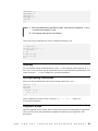
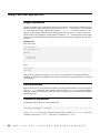
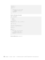
A simple model (volsay.mod)
A typical model is shown here.
dvar float+ Gas;
dvar float+ Chloride;
maximize
40 * Gas + 50 * Chloride;
subject to {
ctMaxTotal:
Gas + Chloride <= 50;
ctMaxTotal2:
3 * Gas + 4 * Chloride <= 180;
10
I B M
I L O G
O P L
L A N G U A G E
R E F E R E N C E
M A N U A L
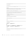
ctMaxChloride:
Chloride <= 40;
}
In this example, there is only the declarative initial part and the model definition. There is
no preprocessing, postprocessing, or flow control.
I B M
I L O G
O P L
L A N G U A G E
R E F E R E N C E
M A N U A L
11
12
I B M
I L O G
O P L
L A N G U A G E
R E F E R E N C E
M A N U A L
Data types
Describes basic data types and data structures available for modeling data in OPL.
In this section
Basic data types
Describes integers, floats, strings, piecewise linear functions, and stepwise functions in
OPL.
Data structures
Describes how the basic data types can be combined using arrays, tuples, and sets to obtain
complex data structures.
I B M
I L O G
O P L
L A N G U A G E
R E F E R E N C E
M A N U A L
13
14
I B M
I L O G
O P L
L A N G U A G E
R E F E R E N C E
M A N U A L
Basic data types
Describes integers, floats, strings, piecewise linear functions, and stepwise functions in
OPL.
In this section
Integers
Describes integers (int) in OPL.
Floats
Describes floats (float) in OPL.
Strings
Describes strings (string) in OPL.
Piecewise linear functions
Describes piecewise linear functions (pwlFunction) in OPL.
Stepwise functions
Describes stepwise functions (stepFunction) in OPL.
I B M
I L O G
O P L
L A N G U A G E
R E F E R E N C E
M A N U A L
15
Integers
Shows how to declare integers in the OPL language.
OPL contains the integer constant maxint, which represents the largest positive integer
available. OPL provides the subset of the integers ranging from -maxint to maxint as a basic
data type.
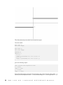
A declaration of the form
int i = 25;
declares an integer, i, whose value is 25.
The initialization of an integer can be specified by an expression. For instance, the declaration
int n = 3;
int size = n*n;
initializes size as the square of n. Expressions are covered in detail in Expressions.
16
I B M
I L O G
O P L
L A N G U A G E
R E F E R E N C E
M A N U A L
Floats
Shows how to declare floats in the OPL language.
OPL also provides a subset of the real numbers as the basic data type float. The
implementation of floats in OPL obeys the IEEE 754 standard for floating-point arithmetic
and the data type float in OPL uses double-precision floating-point numbers. OPL also has
a predefined float constant, infinity, to represent the IEEE infinity symbol. Declarations
of floats are similar to declarations of integers.
The declaration
float f = 3.2;
declares a float f whose value is 3.2.
The value of the float can be specified by an arbitrary expression.
I B M
I L O G
O P L
L A N G U A G E
R E F E R E N C E
M A N U A L
17
Strings
Shows how to declare strings in the OPL language.
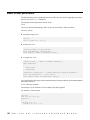
OPL supports a string data type. The excerpt
{string} Tasks = {"
masonry","carpentry","plumbing","ceiling",
"roofing","painting","windows","facade",
"garden","moving"};
defines and initializes a set of strings. Strings can appear in tuples and index arrays.
Strings are manipulated in the preprocessing phase via ILOG Script. See IBM ILOG Script
for OPL for details on the scripting language.
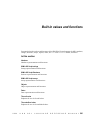
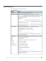
The OPL parser supports the following escape sequences inside literal strings:
Escape sequences inside literal strings
\b
backspace
\t
tab
\n
newline
\f
form feed
\r
carriage return
\"
double quote
\\
backslash
\ooo
octal character ooo
\xXX
hexadecimal character XX
To continue a literal string over several lines, you need to escape the new line character:
"first line \
second line"
18
I B M
I L O G
O P L
L A N G U A G E
R E F E R E N C E
M A N U A L
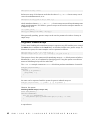
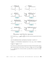
Piecewise linear functions
Shows how to declare piecewise linear functions in the OPL language.
Piecewise linear functions are typically used to model a known function of time, for instance
the cost incurred for completing an activity after a known date.
Note that you must ensure that the array of values T[i] is sorted.
The meanings of the S, T, and V vectors are described in Piecewise linear and stepwise
functions in the Language Reference Manual.
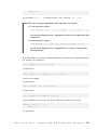
Syntax
pwlFunction F = piecewise(i in 1..n){ S[i]->T[i]; S[n+1] } (t0, v0);
pwlFunction F = piecewise{ V[1]->T[1], ..., V[n]->T[n], V[n+1] };
pwlFunction F[i in ...] = piecewise (...)[ ... ];
Example
int n=2;
float objectiveforxequals0=300;
float breakpoint[1..n]=[100,200];
float slope[1..n+1]=[1,2,-3];
dvar int x;
maximize piecewise(i in 1..n)
{slope[i] -> breakpoint[i]; slope[n+1]}(0,objectiveforxequals0) x;
subject to
{
true;
}
Piecewise linear functions are covered in detail in Piecewise linear and stepwise functions.
I B M
I L O G
O P L
L A N G U A G E
R E F E R E N C E
M A N U A L
19
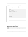
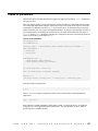
Stepwise functions
Shows how to declare stepwise functions in the OPL language.
Stepwise linear functions are typically used to model the efficiency of a resource over time.
A stepwise function is a special case of piecewise linear function where all slopes are equal
to 0 and the domain and image of F are integer.
Note that you must ensure that the array of values T[i] is sorted.
Syntax
stepFunction F = stepwise(i in 1..n){ V[i]->T[i]; V[n+1] };
stepFunction F = stepwise{ V[1]->T[1], ..., V[n]->T[n], V[n+1] };
stepFunction F[i in ...] = stepwise (...)[ ... ];
Example
A declaration of the form
stepFunction f=stepwise {0->3; 2};
assert f(-1)==0;
assert f(3)==2;
assert f(3.1)==2;
declares a stepwise function, f.
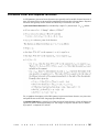
Example
Another example, declaring the stepwise function F2:
stepFunction F2 = stepwise{ 0->0; 100->20; 60->30; 100 };
int ii= F2( 10 );
execute {
writeln( ii );
writeln( F2( 25 ) );
}
Stepwise functions are covered in detail in Piecewise linear and stepwise functions.
20
I B M
I L O G
O P L
L A N G U A G E
R E F E R E N C E
M A N U A L
Data structures
Describes how the basic data types can be combined using arrays, tuples, and sets to obtain
complex data structures.
In this section
Ranges
Describes ranges in OPL.
Arrays
Describes one-dimensional arrays and multidimensional arrays.
Tuples
Describes how to declare tuples, use keys on tuples, initialize tuples. Also indicates the
limitations to which tuples are subject.
Sets
Gives a definition of sets, a list of the operations allowed on sets, and a few words on their
initialization.
Sorted and ordered sets
Shows how sets are sorted and ordered in OPL.
I B M
I L O G
O P L
L A N G U A G E
R E F E R E N C E
M A N U A L
21
Ranges
Integer ranges are fundamental in OPL, since they are often used in arrays and variable
declarations, as well as in aggregate operators, queries, and quantifiers.
Declaring ranges
To specify an integer range, you give its lower and upper bounds, as in
range Rows = 1..10;
which declares the range value 1..10. The lower and upper bounds can also be given by
expressions, as in
int n = 8;
range Rows = n+1..2*n+1;
Once a range has been defined, you can use it as an array indexer:
Whenever a range is empty, i.e. its upper bound is less than its lower bound, it is automatically
normalized to 0..-1 (in other words, all empty ranges are equal).
The range declaration
An integer range is typically used:
♦
as an array index in an array initialization expression
range R = 1..100;
int A[R]; // A is an array of 100 integers
♦
as an iteration range
range R = 1..100;
forall(i in R) {
//element of a loop
...
}
♦
as the domain of an integer decision variable
dvar int i in R;
22
I B M
I L O G
O P L
L A N G U A G E
R E F E R E N C E
M A N U A L
The range float declaration
A range float data type consists of a couple of float values specifying an interval. It is
typically used as the domain of a floating-point decision variable:
range float X = 1.0..100.0;
dvar float x in X;
I B M
I L O G
O P L
L A N G U A G E
R E F E R E N C E
M A N U A L
23
Arrays
Arrays are fundamental in many applications.
One-dimensional arrays
One-dimensional arrays are the simplest arrays in OPL and vary according to the type of
their elements and index sets. A declaration of the form
int a[1..4] = [10, 20, 30, 40];
declares an array of four integers a[1],...,a[4] whose values are 10, 20, 30, and 40. It is
of course possible to define arrays of other basic types. For instance, the instructions
int a[1..4] = [10, 20, 30, 40];
float f[1..4] = [1.2, 2.3, 3.4, 4.5];
string d[1..2] = [“Monday”, “Wednesday”];
declare arrays of natural numbers, floats, and strings, respectively.
The index sets of arrays in OPL are very general and can be integer ranges and arbitrary
finite sets. In the examples so far, index sets were given explicitly, but it is possible to use
a previously defined range, as in
range R = 1..4;
int a[R] = [10, 20, 30, 40];
The declaration:
int a[Days] = [10, 20, 30, 40, 50, 60, 70];
describes an array indexed by a set of strings; its elements are a[“Monday”],...,a
[“Sunday”].
Arrays can also be indexed by finite sets of arbitrary types. This feature is fundamental in
OPL to exploit sparsity in large linear programming applications, as discussed in detail in
Exploiting sparsity in the Language User’s Manual.
For example, the declaration:
tuple Edges {
int orig;
int dest;
}
{Edge} Edges = {<1,2>, <1,4>, <1,5>};
int a[Edges] = [10,20,30];
defines an integer array, a, indexed by a finite set of tuples. Its elements are a[<1,2>], a
[<1,4>], and a[<1,5>]. Tuples are described in detail in Tuples.
24
I B M
I L O G
O P L
L A N G U A G E
R E F E R E N C E
M A N U A L
Multidimensional arrays
OPL supports the declaration of multidimensional arrays (see Data initialization about the
ellipsis syntax). For example, the declaration:
int a[1..2][1..3] = ...;
declares a two-dimensional array, a, indexed by two integer ranges. Indexed sets of different
types can of course be combined, as in
int a[Days][1..3] = ...;
which is a two-dimensional array whose elements are of the form a[Monday][1]. It is
interesting to contrast multidimensional and one-dimensional arrays of tuples.
Consider the declaration:
{string} Warehouses = ...;
{string} Customers = ...;
int transp[Warehouses,Customers] = ...;
that declares a two-dimensional array transp. This array may represent the units shipped
from a warehouse to a customer. In large-scale applications, it is likely that a given warehouse
delivers only to a subset of the customers. The array transp is thus likely to be sparse, i.e.
it will contain many zero values.
The sparsity can be exploited by declarations of the form:
{string} Warehouses ...;
{string} Customers ...;
tuple Route {
string w;
string c;
}
{Route} routes = ...;
int transp[routes] = ... ;
This declaration specifies a set, routes, that contains only the relevant pairs (warehouse,
customer). The array transp can then be indexed by this set, exploiting the sparsity present
in the application. It should be clear that, for large-scale applications, this approach leads
to substantial reductions in memory consumption.
You can initialize arrays by listing its values, as in most of the examples presented so far.
See Initializing arrays, As generic arrays, and As generic indexed arrays for details.
I B M
I L O G
O P L
L A N G U A G E
R E F E R E N C E
M A N U A L
25
Tuples
Data structures in OPL can also be constructed using tuples that cluster together closely
related data.
Declaring tuples
For example, the declaration:
tuple Point {
int x;
int y;
};
Point point[i in 1..3] = <i, i+1>;
declares a tuple Point consisting of two fields x and y of type integer. Once a tuple type T
has been declared, tuples, arrays of tuples, sets of tuples of type T, tuples of tuples can be
declared, as in:
Point p = <2,3>;
Point point[i in 1..3] = <i, i+1>;
{Point} points = {<1,2>, <2,3>};
tuple Rectangle {
Point ll;
Point ur;
}
These declarations respectively declare a point, an array of three points, a set of two points,
and a tuple type where the fields are points. The various fields of a tuple can be accessed
in the traditional way by suffixing the tuple name with a dot and the field name, as in
Point p = <2,3>;
int x = p.x;
which initializes x to the field x of tuple p. Note that the field names are local to the scope
of the tuples.
Note: Multidimensional arrays are not supported in tuples.
Keys in tuple declaration
As in database systems, tuple structures can be associated with keys. Tuple keys enable you
to access data organized in tuples using a set of unique identifiers. In Declaring a tuple
using a single key (nurses.mod), the nurse tuple is declared with the key name of type string.
26
I B M
I L O G
O P L
L A N G U A G E
R E F E R E N C E
M A N U A L
Declaring a tuple using a single key (nurses.mod)
tuple nurse {
key string name;
int seniority;
int qualification;
int payRate;
}
Then, supposing Isabelle must not work more than 20 hours a week, just write:
NurseWorkTime[<"Isabelle">]<=20;
leaving out the fields with no keys. This is equivalent to:
NurseWorkTime[<"Isabelle",3,1,16>]<=20;
Using keys in tuple declarations has practical consequences, in particular:
♦
The key field can be used as a unique identifier for the tuple, for example the field name
in the nurses example in Declaring a tuple using a single key (nurses.mod). In this example,
it means that there will be no two tuples with the same name in a set of tuples of the type
nurse. If a user inadvertently attempts to add two different tuples with the same name,
OPL raises an error.
♦
Defining keys enables you to access elements of the tuple set by using only the value of
the key field (name in the nurses example). Slicing is one of the features that benefit from
it: you can slice on the tuple set using only key fields.
You can also declare a tuple using a non singleton set of keys, such as the shift tuple of
the nurses example in Declaring a tuple using a set of keys (nurses.mod).
Declaring a tuple using a set of keys (nurses.mod)
tuple shift {
key string departmentName;
key string day;
key int startTime;
key int endTime;
int minRequirement;
int maxRequirement;
}
In Declaring a tuple using a set of keys (nurses.mod), a shift is uniquely identified by the
department name, the date, and start and end times, all defined as key fields.
Initializing tuples
You initialize tuples by giving the list of the values of the various fields, as in:
Point p = <2,3>;
which initializes p.x to 2 and p.y to 3. See Initializing tuples for details.
I B M
I L O G
O P L
L A N G U A G E
R E F E R E N C E
M A N U A L
27
Limitations on tuples
When using tuples in your models, you should be aware of various limitations.
Data types in tuples
Not all data types are allowed inside tuples. The limitations are given here.
Data types allowed in tuples
♦
Primitives (int, float, string)
♦
Tuples (also known as subtuples)
♦
Arrays with primitive items (not string), that is: integer or float arrays
♦
Sets with primitive items, that is: integer, float or string sets
Data types not allowed in tuples
♦
Sets of tuples (instances of IloTupleSet)
♦
Arrays of strings, tuples, and tuple sets
♦
Multidimensional arrays
Tuple indices and tuple patterns
You cannot mix tuple indexes and patterns within the declaration and the use of decision
expressions. For example, these code lines raise the following error message Data not
consistent for "xxx": can not mix pattern and index between declaration of
dexpr and instantiation.
Do not mix tuple indices and tuple patterns in dexpr
dexpr float y[i in t] = ...;
subject to {
forall(<a,b,c> in t) y[<a,b,c>]==...; };
dexpr float y[<a,b,c> in t] = ...;
subject to {
forall(i in t) y[i]==...;
};
Performance and memory consumption
If you choose to label constraints in large models, use tuple indices instead of tuple patterns
to avoid increasing the performance and memory cost. See Constraint labels.
28
I B M
I L O G
O P L
L A N G U A G E
R E F E R E N C E
M A N U A L
Sets
Definition
Sets are non-indexed collections of elements without duplicates.
OPL supports sets of arbitrary types to model data in applications. If T is a type, then {T},
or alternatively setof(T), denotes the type “set of T”. For example, the declaration:
{int} setInt = ...;
setof(Precedence) precedences = ...;
declares a set of integers and a set of precedences.
Sets may be ordered, sorted, or reversed. By default, sets are ordered, which means that:
♦
Their elements are considered in the order in which they have been created.
♦
Functions and operations applied to ordered sets preserve the order.
See Sorted and ordered sets for details.
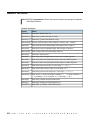
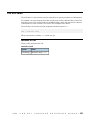
Operations on sets
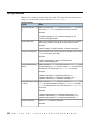
The following operations are allowed on sets. See OPL functions in Language Quick Reference
for more information about functions. For the functions on sets, the index starts at 0.
Operations allowed on sets
Operations
Syntax
union, inter, diff, symdiff
set = function(set1,set2)
first, last
elt = function(set)
next, prev
elt = function(set,elt,int)
nextc, prevc
elt = function(set,elt,int)
item
elt = function(set,int)
ord
int = function(set,elt)
Initializing sets
A set can be initialized in various ways. The simplest way is by listing its values explicitly.
For example:
tuple Precedence {
int before;
int after;
I B M
I L O G
O P L
L A N G U A G E
R E F E R E N C E
M A N U A L
29
}
{Precedence} precedences = {<1,2>, <1,3>, <3,4>};
See Initializing sets for details.
30
I B M
I L O G
O P L
L A N G U A G E
R E F E R E N C E
M A N U A L
Sorted and ordered sets
Sets can be either sorted or ordered:
♦
An ordered set is a set which elements are arranged in the order in which they were
added to the set. Note that this is how sets are created by default. For example:
{int} S1 = {3,2,5};
and
ordered {int} S1 = {3,2,5};
are equvalent.
♦
A sorted set is a set in which elements are arranged in their natural, ascending order.
For strings, the natural order is the lexicographic order. The natural order also depends
on the system locale. To specify the descending order, you add the keyword reversed.
For example:
sorted {int} sortedS = {3,2,5};
and
ordered {int} orderedS = {2,3,5};
are equvalent, and iterating over sortedS or orderedS will have the same behavior.
This section shows the effect of the sorted property on simple sets, tuple sets, and sets used
in piecewise linear functions.
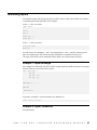
Simple sets
The code sample Sorted sets enables you to see the difference between the union of ordered
sets and the union of sorted sets.
Sorted sets
{int} s1 = {3,5,1};
{int} s2 = {4,2};
{int} orderedS = s1 union s2;
sorted {int} sortedS = s1 union s2;
execute{
writeln("ordered union = ", orderedS);
writeln("sorted union = ", sortedS);
}
The statement
{int} orderedS = s1 union s2;
returns
ordered union =
I B M
I L O G
O P L
{3 5 1 4 2}
L A N G U A G E
R E F E R E N C E
M A N U A L
31
while the statement
sorted {int} sortedS = s1 union s2;
returns
sorted union =
{1 2 3 4 5}
Sorted tuple sets
When a tuple set uses no keys, the entire tuple, except set and array fields, is taken into
account for sorting. For tuple sets with keys, sorting takes place on all keys in their order
of declaration. In other words, it is not possible to sort a tuple set on one (or more) given
column(s) only.
The code extract below, Sorted tuple sets, declares a team of people who are defined by
their first name, last name, and nickname, then prints the list of team members first in the
creation order, then in alphabetical order.
Sorted tuple sets
tuple person {
string firstname;
string lastname;
string nickname;
}
tuple personKeys {
key string firstname;
key string lastname;
string nickname;
}
{person} devTeam = {
<"David", "Atkinson", "Dave">,
<"David", "Doe", "Skinner">,
<"Gregory", "Simons", "Greg">,
<"David", "Smith", "Lewis">,
<"Kevin", "Morgan", "Kev">,
<"Gregory", "McNamara ", "Mac">
};
sorted {personKeys} sortedDevTeam = {<i,j,k> | <i,j,k> in devTeam};
execute{
writeln(devTeam);
writeln(sortedDevTeam);
}
The person tuple uses no keys.
tuple person {
string firstname;
string lastname;
string nickname;
}
The personKeys tuple uses keys for the first and last names, not for the nickname.
32
I B M
I L O G
O P L
L A N G U A G E
R E F E R E N C E
M A N U A L
tuple personKeys {
key string firstname;
key string lastname;
string nickname;
}
The data shows that the team includes three people whose first name is David, two people
whose first name is Gregory, and one person whose first name is Kevin.
As a consequence, the statement
sorted {personKeys} sortedDevTeam = {<i,j,k> | <i,j,k> in devTeam};
lists the David tuples before the Gregory tuples, which themselves appear before the Kevin
tuple. Within the David tuples, "David" "Doe" "Skinner" comes before "David" "Smith"
"Lewis" because a second sorting also takes place on the second field with the key lastname.
In contrast, since there is no person with the same first name and last name, no sort is ever
done on the last field nickname.
The output of sortedDevTeam is displayed in the OPL IDE as:
{<"David" "Atkinson" "Dave"> <"David" "Doe" "Skinner">
<"David" "Smith" "Lewis"> <"Gregory" "McNamara " "Mac">
<"Gregory" "Simons" "Greg"> <"Kevin" "Morgan" "Kev">}
Sorted sets in piecewise linear functions
In piecewise linear functions, breakpoints must be strictly increasing. However, in most
cases, the data supplied by a database or a .dat file is not sorted in an increasing numeric
or lexicographic order. As a consequence, you have to add complex and verbose scripting
statements to sort the data.
To avoid these extra code lines, the sorted property of sets enables you to sort data by
specifying a single keyword, as shown in the code extract below, Piecewise linear function
with sorted sets. Writing piecewise linear functions becomes easier, as one code line is
sufficient instead of several dozens.
Piecewise linear function with sorted sets
tuple Cost{
key int BreakPoint;
float Slope;
}
sorted {Cost} sS = { <1, 1.5>, <0, 2.5>, <3, 4.5>, <2, 4.5>};
float lastSlope = 3.5;
dvar float+ x;
minimize piecewise(t in sS)
{t.Slope -> t.BreakPoint; lastSlope} x;
See also Piecewise-linear functions.
I B M
I L O G
O P L
L A N G U A G E
R E F E R E N C E
M A N U A L
33
For more information
See Data sources to learn about data initialization.
See Introduction to scripting of the Language User’s Manual on how to set declarations.
34
I B M
I L O G
O P L
L A N G U A G E
R E F E R E N C E
M A N U A L
Data sources
Describes data and database initialization, spreadsheet input/output, data consistency, and
preprocessing.
In this section
Data initialization
Defines internal versus external initialization, describes how to initialize arrays, tuples, and
sets, and discusses memory allocation aspects of data initialization.
Database initialization
Describes how to connect to one or several relational databases, how to read from such
databases using traditional SQL queries, and to write the results back to the connected
database.
Spreadsheet Input/Output
Describes how to connect an MS Excel spreadsheet, read from it, and write the results to
the connected spreadsheet.
Data consistency
Defines the purpose of data consistency and describes data membership and assertions as
ways to ensure consistency.
Preprocessing data
Provides an overview of preprocessing operations in OPL.
I B M
I L O G
O P L
L A N G U A G E
R E F E R E N C E
M A N U A L
35
36
I B M
I L O G
O P L
L A N G U A G E
R E F E R E N C E
M A N U A L
Data initialization
Defines internal versus external initialization, describes how to initialize arrays, tuples, and
sets, and discusses memory allocation aspects of data initialization.
In this section
Internal vs. external initialization
Defines these two kinds of data initialization.
Initializing arrays
Describes the various ways in which you can initialize arrays.
Initializing tuples
Describes the two ways of initializing tuples.
Initializing sets
Describes the three ways of initializing sets.
Initialization and memory allocation
Describes how memory is allocated to data initialization.
I B M
I L O G
O P L
L A N G U A G E
R E F E R E N C E
M A N U A L
37
Internal vs. external initialization
In OPL, you can initialize data internally or externally. Your choice affects memory allocation.
See Initialization and memory allocation for details.
Internally
This initialization mode consists in initializing the data in the model file at the same time as
it is declared. Inline initializations can contain expressions to initialize data items, such as
int a[1..5] = [b+1, b+2, b+3, b+4, b+5];
Note: If you choose to initialize data within a model file, you will get an error message if you
try to access it later by means of a scripting statement such as:
myData.myArray_inMod[1] = 2;
Externally
This initialization mode consists in specifying initialization subsequently as an OPL statement
in a separate .dat file (see OPL Syntax in the Language Quick Reference). This includes
reading from a database, as explained in Database initialization, or from a spreadsheet as
explained in Spreadsheet Input/Output.
You declare external data using the ellipsis syntax. However, data initialization instructions
cannot contain expressions, since they are intended to specify data. Data initialization
instructions make it possible to specify sets of tuples in very compact ways. Consider these
types in a .mod file:
{string} Product ={"flour", "wheat", "sugar"};
{string} City ={"Providence", "Boston", "Mansfield"};
tuple Ship {
string orig;
string dest;
string p;
}
{Ship} shipData = ...;
and assume that the set of shipments is initialized externally in a separate .dat file like this:
shipData =
{
<"Providence",
<"Providence",
<"Providence",
<"Providence",
38
I B M
I L O G
O P L
"Boston",
"Boston",
"Boston",
"Boston",
"wheat">
"flour">
"sugar">
"wheat">
L A N G U A G E
R E F E R E N C E
M A N U A L
<"Providence", "Mansfield", "wheat">
<"Providence", "Mansfield", "flour">
<"Boston", "Providence", "sugar">
<"Boston", "Providence", "flour">
};
Note: In .dat files, the separating comma is optional. For strings without any special
characters, even the enclosing quotes are optional.
I B M
I L O G
O P L
L A N G U A G E
R E F E R E N C E
M A N U A L
39
Initializing arrays
You can initialize arrays:
♦
Externally
♦
Internally
♦
In preprocessing instructions
♦
As generic arrays
♦
As generic indexed arrays
Externally
Arrays can be initialized by external data, in which case the declaration has the form:
int a[1..2] [1..3] = ...;
and the actual initialization is given in a data source, which is a separate .dat file in IBM
ILOG OPL.
Listing values
This is how arrays are initialized in most of the examples presented so far. Multidimensional
arrays in OPL are, in fact, arrays of arrays and must be initialized accordingly. For example,
the declaration:
/* .mod file */
int a[1..2][1..3] = ...;
/* .dat file */
a = [
[10, 20, 30],
[40, 50, 60]
];
initializes a two-dimensional array by giving initializations for the one-dimensional arrays
of its first dimension. It is easy to see how to generalize this initialization to any number of
dimensions.
Specifying pairs
An array can also be initialized by specifying pairs (index, value), as in the declaration:
/* .mod file */
int a[Days] = ...;
/* .dat file */
a = #[
“Monday”: 1,
”Tuesday”: 2,
40
I B M
I L O G
O P L
L A N G U A G E
R E F E R E N C E
M A N U A L
”Wednesday”: 3,
”Thursday”: 4,
”Friday”: 5,
”Saturday”: 6,
”Sunday”: 7
]; #
Note: 1. When the initialization is specified by (index, value) pairs, the delimiters #[ and ]
# must be used instead of [ and ].
2. The ordering of the pairs can be arbitrary.
These two forms of initialization can be combined arbitrarily, as in:
/* .mod file */
int a[1..2][1..3] = ...;
/* .dat file */
a = #[
2: [40, 50, 60],
1: [10, 20, 30]
]#;
Internally
You can initialize arrays internally (that is, in the .mod file) using the same syntax as in .dat
files. Here, the array items may be expressions that are evaluated during initialization. The
syntax for pairs #[, ]# is not available for internal initialization.
In preprocessing instructions
Arrays can also be initialized in the preprocessing instructions, as in:
range R = 1..8;
int a[R];
execute {
for(var i in R) {
a[i] = i + 1;
}}
which initializes the array in such a way that a[1] = 2, a[2] = 3, and so on.
See Preprocessing data.
As generic arrays
OPL also supports generic arrays, that is, arrays whose items are initialized by an expression.
These generic arrays may significantly simplify the modeling of an application. The
declaration:
I B M
I L O G
O P L
L A N G U A G E
R E F E R E N C E
M A N U A L
41
int a[i in 1..10] = i+1;
declares an array of 10 elements such that the value of a[i] is i+1. Generic arrays can of
course be multidimensional, as in:
int m[i in 0..10][j in 0..10] = 10*i + j;
which initializes element m[i][j] to 10*i + j. Generic arrays are useful in performing some
simple transformations. For instance, generic arrays can be used to transpose matrices in
a simple way, as in:
int m[Dim1][Dim2] = ...;
int t[j in Dim2][i in Dim1] = m[i][j];
More generally speaking, generic arrays can be used to permute the indices of arrays in
simple ways.
As generic indexed arrays
To have more flexibility when initializing arrays in a generic way, OPL enables you to control
the index value in addition to the item value, as described earlier in As generic arrays. To
illustrate the syntax, the same examples can be expressed as follows:
int a[1..10] = [ i-1 : i | i in 2..11 ];
int m[0..10][0..10] = [ i : [ j : 10*i+j ] | i,j in 0..10 ];
This syntax is close to the syntax used for initializing arrays in .dat files by means of indices,
delimited by #[ and ] #, as explained in Specifying pairs. Using this syntax is an efficient
means of initializing arrays used to index data.
The oilDB.mod example contains an execute block that performs initialization. Instead of:
GasType gas[Gasolines];
execute {
for(var g in gasData) {
gas[g.name] = g
}
}
the same can be expressed with the syntax for generic indexed arrays as:
GasType gas[Gasolines] = [ g.name : g | g in gasData ];
Likewise, this syntax:
Initializing indexed arrays (transp4.mod)
float Cost[Routes];
execute INITIALIZE {
for( var t in TableRoutes ) {
Cost[Routes.get(t.p,Connections.get(t.o,t.d))] = t.cost;
}
}
is equivalent to:
42
I B M
I L O G
O P L
L A N G U A G E
R E F E R E N C E
M A N U A L
float Cost[Routes] = [ <t.p,<t.o,t.d>>:t.cost | t in TableRoutes ];
Note: 1. It is recommended to use generic arrays or generic indexed arrays whenever
possible, since they make the model more explicit and readable.
2. If an index is met more than once, no warning is issued and the latest value set
for this index is the one kept.
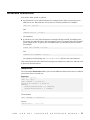
For example:
int n=5;
{int} s= {1,3,4,2,5};
sorted {int} s2=asSet(1..n);;
reversed {int} s3=asSet(1..n);;
int x[1..n]=[maxl(n-i,i): i | i in s];
int x2[1..n]=[maxl(n-i,i): i | i in s2];
int x3[1..n]=[maxl(n-i,i): i | i in s3];
execute
{
writeln(x);
writeln(x2);
writeln(x3);
}
gives out
[0 0 2 4 5]
[0 0 3 4 5]
[0 0 2 1 5]
From a database
Reading database columns to a tuple array (oilDB2.dat) is more efficient since no data is
duplicated.
Reading database columns to a tuple array (oilDB2.dat)
Gasolines,Gas from DBRead(db,"SELECT name,name,demand,price,octane,lead FROM
GasData");
Oils,Oil from DBRead(db,"SELECT name,name,capacity,price,octane,lead FROM
OilData");
You can also write:
Gasolines from DBRead(db,"SELECT name FROM GasData");
Gas from DBRead(db,"SELECT name,demand,price,octane,lead FROM GasData");
I B M
I L O G
O P L
L A N G U A G E
R E F E R E N C E
M A N U A L
43
Oils from DBRead(db,"SELECT name from OilData");
Oil from DBRead(db,"SELECT name,capacity,price,octane,lead FROM OilData");
44
I B M
I L O G
O P L
L A N G U A G E
R E F E R E N C E
M A N U A L
Initializing tuples
You initialize tuples either by giving the list of the values of the various fields (see Tuples)
or by listing the fields and values. For example:
In the .mod file, you write:
tuple point
{
int x;
int y;
}
point p1=...;
point p2=...;
In the .dat file, you write:
p1=#<y:1,x:2>#;
p2=<2,1>;
As with arrays, the delimiters < and > are replaced by #< and ># and the ordering of the
pairs is not important. OPL checks whether all fields are initialized exactly once.
The type of the fields can be arbitrary and the fields can contain arrays and sets.
Example 1: tuple Rectangle
For example, the following code lines declare a tuple with three fields: the first is an integer
and the other two are arrays of two points.
tuple Rectangle {
int id;
int x[1..2];
int y[1..2];
}
Rectangle r = ...;
execute
{
writeln(r);
}
A specific “rectangle” can be declared in the data file as:
r=<1, [0,10], [0,10]>;
Example 2: tuple Precedence
The declaration
I B M
I L O G
O P L
L A N G U A G E
R E F E R E N C E
M A N U A L
45
tuple Precedence {
string name;
{string} after;
}
defines a tuple in which the first field is a set item and the second field is a set of values. A
possible precedence can be declared as follows:
Precedence p = <a1, {a2, a3, a4, a5}>;
assuming that a1,..,a5 are strings.
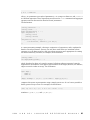
You can also initialize tuples internally within the .mod file. If you choose to do so, you cannot
use the named tuple component syntax #<, >#, which is supported in .dat files but not in
.mod files. Components may be expressions and will be evaluated during initialization.
46
I B M
I L O G
O P L
L A N G U A G E
R E F E R E N C E
M A N U A L
Initializing sets
You can initialize sets:
♦
Externally
♦
Internally
♦
As generic sets
Externally
As stated in Initializing sets, the simplest way to initialize a set is by listing its values explicitly
in the .dat file.
For example, the declaration:
/* .mod file */
tuple Precedence {
int before;
int after;
}
{Precedence} precedences = ...;
/* .dat file */
precedences = {<1,2>, <1,3>, <3,4>};
initializes a set of tuples.
Internally
You can also initialize sets internally (in the .mod file), more precisely by using set expressions
using previously defined sets and operations such as union, intersection, difference, and
symmetric difference. The symmetric difference of two sets A and B is
(A union symbol B) \ (A intersection symbol B)
described in Expressions.
For example, the declarations:
{int}
{int}
{int}
{int}
{int}
{int}
{int}
s1 = {1,2,3};
s2 = {1,4,5};
i = s1 inter s2;
j = {1,4,8,10} inter s2;
u = s1 union {5,7,9};
d = s1 diff s2;
sd = s1 symdiff {1,4,5};
initialize i to {1}, u to {1,2,3,5,7,9}, d to {2,3}, and sd to {2,3,4,5}.
It is also possible to initialize a set from a range expression. For example, the declaration:
I B M
I L O G
O P L
L A N G U A G E
R E F E R E N C E
M A N U A L
47
{int} s = asSet(1..10)
initializes s to {1,2,..,10}
It is important to point out at this point that sets initialized by ranges are represented
explicitly (unlike ranges). As a consequence, a declaration of the form
{int} s = asSet(1..100000);
creates a set where all the values 1, 2, ..., 100000 are explicitly represented, while the range
range s = 1..100000;
represents only the bounds explicitly.
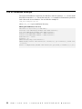
More about internal initialization of sets
When writing the assignment s2=s1, you add one element to s1, that element is also added
to s2. If you do not want this, write
s1={i|i in s2}
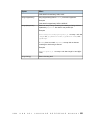
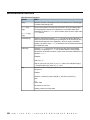
For example, compare the statements in Initializing sets in the model file:
Initializing sets in the model file
If you write {int} s1={1,2}; {int} s1={1,2};
{int} s2=s1;
{int} s2={ i | i in s1};
execute
//{int} s2=s1;
{
execute
s2.add(3);
{
writeln(s1);
s2.add(3);
}
writeln(s1);
}
the result is {1 2 3}
{1 2}
As generic sets
OPL supports generic sets which have an expressive power similar to relational database
queries. For example, the declaration:
{int} s = {i | i in 1..10: i mod 3 == 1};
initializes s with the set {1,4,7,10}. A generic set is a conjunction of expressions of the
form
48
I B M
I L O G
O P L
L A N G U A G E
R E F E R E N C E
M A N U A L
p in S : condition
where p is a parameter (or a tuple of parameters), S is a range or a finite set, and condition
is a Boolean expression. These expressions are also used in forall statements and aggregate
operators and are discussed in detail in Formal parameters.
The declaration:
{string} Resources ...;
{string} Tasks ...;
Tasks res[Resources] = ...;
tuple Disjunction {
{string} first;
{string} second;
}
{Disjunction} disj = {<i,j> |
r in Resources, ordered i,j in res[r]
};
is a more interesting example, showing a conjunction of expressions, and is explained in
detail in Formal parameters. Generic sets are often useful when you transform a data
structure (e.g. the data stored in a file) into a data structure more appropriate for stating
the model effectively. Consider, for example, the declarations:
{string} Nodes ...;
int edges[Nodes][Nodes] = ...;
which describe the edges of a graph in terms of a Boolean adjacency matrix. It may be
important for the model to use a sparse representation of the edges (because, for instance,
edges are used to index an array). The declaration:
tuple Edge {
Nodes o;
Nodes d;
}
{Edge} setEdges = {<o,d> | o,d in Nodes : edges[o][d]==1};
computes this sparse representation using a simple generic set. It is of course possible to
define generic arrays of sets. For example, the declaration:
{int} a[i in 3..4] = {e | e in 1..10: e mod i == 0};
initializes a[3] to {3,6,9} and a[4] to {4,8}.
I B M
I L O G
O P L
L A N G U A G E
R E F E R E N C E
M A N U A L
49
Initialization and memory allocation
In OPL, the initialization mode you choose affects memory allocation. Namely, external
initialization from a .dat file, while enabling a more modular design, may have a significant
impact on memory usage.
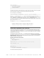
Internal initialization
Internal data (directly from the model file) is initialized when first used. This is also called
“lazy initialization”. Unused internal data elements are not allocated any memory. In other
words, internal data is “pulled” from OPL as needed.
Example of lazy initialization
int a=2;
int b=2;
int a2=2*a;
int b2=2*b;
execute
{
a2;
a++;
b++;
writeln(a2);
writeln(b2);
}
assert a2==4;
assert b2==6;
External initialization
In contrast, data from a data file is initialized while the .dat file is parsed and is allocated
memory whether it is used by the model or not. In other words, external data is “pushed”
to OPL.
50
I B M
I L O G
O P L
L A N G U A G E
R E F E R E N C E
M A N U A L
Database initialization
Describes how to connect to one or several relational databases, how to read from such
databases using traditional SQL queries, and to write the results back to the connected
database.
In this section
The oil database example
Explains database initialization in the context of an oil database.
Supported databases
Provides a reference of the databases supported by OPL.
Connection to a database
Shows how to connect OPL to a database.
Reading from a database
Explains the process of reading data from a database in OPL.
Writing to a database
Explains the process of writing to a database from OPL.
I B M
I L O G
O P L
L A N G U A G E
R E F E R E N C E
M A N U A L
51
The oil database example
The syntax for databases is valid only for data files, with the extension .dat, not for model
files with the extension .mod. This section uses the oilDB example to demonstrate operations
with a Microsoft Access database. You can find this example in
<OPL_dir>/examples/opl/oil
where <OPL_dir> is your installation directory.
Working with databases (oilDB.dat)
DBConnection db("access","oilDB.mdb");
Gasolines from DBRead(db,"SELECT name FROM GasData");
Oils from DBRead(db,"SELECT name FROM OilData");
GasData from DBRead(db,"SELECT * FROM GasData");
OilData from DBRead(db,"SELECT * FROM OilData");
MaxProduction = 14000;
ProdCost = 4;
DBExecute(db,"drop table Result");
DBExecute(db,"create table Result(oil varchar(10), gas varchar(10), blend real,
a real)");
Result to DBUpdate(db,"INSERT INTO Result(oil,gas,blend,a) VALUES(?,?,?,?)");
52
I B M
I L O G
O P L
L A N G U A G E
R E F E R E N C E
M A N U A L
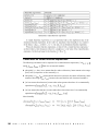
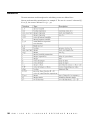
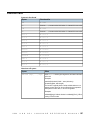
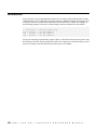
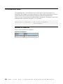
Supported databases
Supported databases in the Working Environment document provides a list of the databases
to which you can connect your OPL model to read and write data.
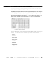
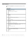
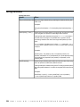
The table below gives the syntax of the string you must use to connect to each of the
supported databases. See The oil database example in IDE Tutorials for details on how to
customize the oil database example for connection to a different database.
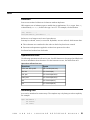
Database connection strings
Database
Name
Connection String
DB2
username/password/database
(The client configuration will find the server.)
I B M
MS SQL
userName/password/database/dbServer
ODBC
dataSourceName/userName/password
Oracle 9 and
later
userName/password@dbInstance
OLE DB
<user>/<password>/<database name>/<server name>
I L O G
O P L
L A N G U A G E
R E F E R E N C E
M A N U A L
53
Connection to a database
In OPL, database operations all refer to a database connection. Here are two examples from
the oilDB example for declaring connections. See Supported databases for more connection
strings.
DBConnection db("odbc","oilDB/user/passwd");
and
DBConnection db("access","oilDB.mdb");
The first example uses the ODBC data source oilDB declared by the system to connect to
the database.
The connection db should be viewed as a handle on the database.
Note: 1. The user and passwd parameters are optional: you can connect to oilDB//
without a user name and password.
2. It is possible to connect to several databases within the same model.
54
I B M
I L O G
O P L
L A N G U A G E
R E F E R E N C E
M A N U A L
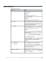
Reading from a database
In OPL, database relations can be read into sets or arrays. For instance, these instructions
from the model file:
tuple gasType {
string name;
float demand;
float price;
float octane;
float lead;
}
tuple oilType {
string name;
float capacity;
float price;
float octane;
float lead;
}
And these instructions from the data file:
GasData from DBRead(db,"SELECT * FROM GasData");
OilData from DBRead(db,"SELECT * FROM OilData");
Together illustrate how to initialize a set of tuples from the relation OilData in the database
db. In this example, the DBRead instruction inserts an element into the set for each tuple of
the relations.
Important conventions adopted by OPL:
1. If read into a set, the resulting set must be a set of integers, floats, or strings, or a set
of tuples whose elements are integers, floats, or strings.
2. If read into an array, the resulting array must be an array of integers, floats, or strings,
or an array of tuples whose elements are integers, floats, or strings.
3. In the case of tuples, the columns of the SQL query result are mapped by position to
the field of the OPL tuples. For instance, in the above query, the column name has been
mapped to the field name and so on.
4. When initializing an array with a DBRead statement, the indexing set and array cells
are initialized at the same time.
Note: OPL does not parse the query; it simply sends the string to the database system that
has full responsibility for handling it. As a consequence, the syntax and the semantics
of these queries are outside the scope of this book and users should consult the
appropriate database manual for more information.
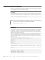
It is also possible to implement parameterized queries in OPL, for example:
I B M
I L O G
O P L
L A N G U A G E
R E F E R E N C E
M A N U A L
55
Oils from DBRead(db,"SELECT name FROM OilData WHERE quality>?")(oilQuality);
where oilQuality is any scalar OPL data element already initialized and whose type is
expected in the SQL query. In this case, oilQuality should be a numeric type, for example
an integer.
Note: Despite standardization, Oracle does not support the question mark as a variable
identifier. Use ':'<parameter number> instead. Examples are ':1', ':arg', etc.
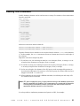
SQL encryption
In OPL 3
Because all database instructions were in the model file, the SQL statements were encrypted
as well when the model was compiled.
In OPL4 and later
To do the same in OPL 4.x (where you write database instructions in data files), you can
define literal strings inside the model file (which will be compiled) and use them in the data
file, like this:
In the .mod file:
string connectionString = "scott/tiger@TEST";
string myQuery = "select id from table";
{int} setOfInt = ...;
dvar int X in 1..5;
minimize X;
subject to {
forall (i in setOfInt)
X >= i;
};
In the .dat file:
DBconnection db("oracle9", connectionString);
setOfInt from DBread (db, myQuery);
56
I B M
I L O G
O P L
L A N G U A G E
R E F E R E N C E
M A N U A L
Writing to a database
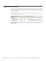
Writing to a database to update it mostly follows the same lines.
Publishing results to a database is similar to parameterized data initialization. Here is an
example extracted from the oil code sample:
All database publishing requests are carried out during postprocessing, if a solution is
available. Such requests are processed in the order declared in the .dat file(s). If your
RDMBS supports transactions, every single publishing request is sent within its own
transaction.
Adding rows
To add rows:
1. Write in the model file:
tuple result {
string oil;
string gas;
float blend;
float a;
}
{result} Result =
{ <o,g,Blend[o][g],a[g]> | o in Oils, g in Gasolines };
2. Write in the data file:
DBExecute(db,"drop table Result");
DBExecute(db,"create table Result(oil varchar(10), gas varchar(10), blend
real, a real)");
Result to DBUpdate(db,"INSERT INTO Result(oil,gas,blend,a) VALUES(?,?,?,?)
");
In this example, you use:
♦
a DBExecute statement to send SQL DDL (data definition language) instructions to the
Relational Database Management Server (RDBMS)
♦
a DBUpdate statement to modify the data (see Updating existing rows).
More generally, the keyword DBExecute enables you to carry out administration tasks on
data tables, whereas the keyword DBUpdate modifies the contents of data tables.
The OPL result publisher will iterate on the items in the set result and bind the component
values to the SQL statement parameters in the declared order.
Note: OPL supports the same element types for reading as for database publishing.
I B M
I L O G
O P L
L A N G U A G E
R E F E R E N C E
M A N U A L
57
Updating existing rows
To update existing rows in a database instead of adding new ones, use an SQL update
statement.
For example, to multiply by 2 the blends for Super:
1. Add the following lines in the .mod file:
tuple Result2 {
float blend;
float a;
string oil;
string gas;
}
{Result2} result2 = { <2*blend[o]["Super"],a["Super"],o,"Super"> | o in
Oils};
2. Write an SQL update statement like this:
result2 to DBUpdate(db,
"UPDATE Result SET blend=? , a=? WHERE oil=? AND gas=?");
See also Getting the data elements from an IloOplModel instance in the Language User’s
Manual for details about data publishers and postprocessing.
Deleting elements
It is also possible to delete elements from a database. For instance, the instructions
/* .mod file */
{string} NamesToDelete = ...;
/* .dat file */
NamesToDelete to DBUpdate(db,"delete from PEOPLE where NAME = ?");
delete from the relation table PEOPLE all the tuples whose names are in NamesToDelete.
Note: The syntax of the actual queries may differ from one database system to another.
58
I B M
I L O G
O P L
L A N G U A G E
R E F E R E N C E
M A N U A L
Spreadsheet Input/Output
Describes how to connect an MS Excel spreadsheet, read from it, and write the results to
the connected spreadsheet.
In this section
The oilsheet example
Explains spreadsheet input and output in the context of an oil spreadsheet.
Connection to a spreadsheet
Explains how to connect OPL to a spreadsheet.
Reading from a spreadsheet
Explains how to read from a spreadsheet from within OPL.
Writing to a spreadsheet
Explains how to write to a spreadsheet from within OPL.
I B M
I L O G
O P L
L A N G U A G E
R E F E R E N C E
M A N U A L
59
The oilsheet example
This section uses the oilSheet example to demonstrate operations with an MS Excel
spreadsheet. You can find this example in
<OPL_dir>/examples/opl/oil
where <OPL_dir> is your installation directory.
Using spreadsheets through ODBC
If you access spreadsheet data through an ODBC connection using a JDBC-ODBC client, the
ODBC driver returns NULL if the data is not of the right type instead of reporting a specific
data type error. See http://support.microsoft.com/kb/194124/EN-US/ for details.
60
I B M
I L O G
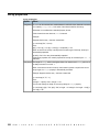
O P L
L A N G U A G E
R E F E R E N C E
M A N U A L
Connection to a spreadsheet
The spreadsheet operations in OPL all refer to a spreadsheet connection. The instruction
/* .dat file */
SheetConnection sheet("transport.xls");
establishes a connection sheet to a spreadsheet named transport.xls. The connection
sheet should be viewed as a handle on the spreadsheet. Note that it is possible in OPL to
connect to several spreadsheets within the same model.
Note that SheetConnection takes only one parameter and that you don't need to specify
the full path to the spreadsheet name. Relative paths are resolved using the current directory
of .dat files.
Note: In this section, we often use the word “spreadsheet” for “spreadsheet connection”.
I B M
I L O G
O P L
L A N G U A G E
R E F E R E N C E
M A N U A L
61
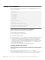
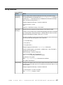
Reading from a spreadsheet
In OPL, spreadsheet ranges can be read into one- or two-dimensional arrays or sets. For
instance, the instructions:
/* .mod file */
{string} Gasolines = ...;
tuple GasType {
float demand;
float price;
float octane;
float lead;
}
GasType gas[Gasolines] = ...;
/* .dat file */
SheetConnection sheet("oilSheet.xls");
Gasolines from SheetRead(sheet,"gas!A2:A4");
gas from SheetRead(sheet,"gas!B2:E4");
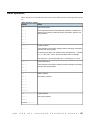
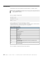
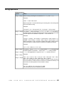
What data can be read from an Excel spreadsheet
OPL opens a spreadsheet in read-only mode to read data from it.
The types of data elements supported are:
♦
sets with integers, floats, strings, or tuples;
♦
scalar integers, floats, or strings;
♦
arrays with integers, floats, one- or two-dimensional strings, or one-dimensional tuples;
♦
one- or two-dimensional arrays of simple types: for such arrays, the data must be
formatted, that is, it must have the same width/length as the array to be filled. OPL
automatically determines whether the data must be read line by line or column by column.
When facing a square zone (a two-dimensional array with [x][x] as dimensions), the
engine reads the data line by line.
Only tuples with integer, float, and string components are supported.
Accessing named ranges in Excel
IBM ILOG OPL supports the convention of names, which are a word or string of characters
used to represent a cell, range of cells, formula, or constant value, and that can be used in
other formulas.
Thus you can use easy-to-understand names, such as Nutrients, to refer to
hard-to-understand ranges, such as B4:J15 or IncreasedProtein to refer to a constraint.
You can then substitute these names in formulas for the range of cells or constraint.
62
I B M
I L O G
O P L
L A N G U A G E
R E F E R E N C E
M A N U A L
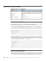
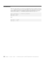
Excel named ranges can be accessed using the SheetRead command, using the following
syntax:
SheetConnection sheetData("C:\ILOG_Files\myExcelFile.xls", 1);
prods from SheetRead(sheetData,"Product");
The SheetRead command is normal, and in this example the Excel name Product replaces
the normal syntax of, say, C13:O72.
To create named ranges in Excel 2003:
1. Highlight the range of cells you want to name, then choose Insert > Name > Define
from the main menu.
2. Type the name you want to assign to this range and click OK.
3. Save the spreadsheet file.
To create named ranges in Excel 2007:
1. Highlight the range of cells you want to name, then click the Name box at the left end
of the Formula Bar.
2. Type the name you want to assign to this range and press Enter.
3. Save the spreadsheet file.
Additional information on named ranges
♦ Excel automatically updates (expands) a named range when a row is added somewhere
within the range. However, one must careful adding rows at the end of a range as the
range does not get automatically updated in that case. It would have to be updated
manually.
♦
OPL allows blank rows in a named range. If you are reading a set of strings, it will consider
the blank cells as having the value 0. If you are reading a set of strings, then it inserts
an empty string "" into the set. For example:
s2 = {"Monday" "" "Wednesday" "Thursday" "Friday"}
This behavior is the same when you don't use named range but instead use explicit ranges
like C1:C5, where C2 is empty.
♦
With the Excel VBA one can name the first (top left) cell of a named range and access
the whole range. OPL does not support this.
♦
When using sheetWrite to write to named ranges, the size of the range does not have to
match the size of the data you are writing to Excel. If the set is smaller, then only the top
most cells will be filled.
If you try to write more data than the range can accommodate, then you receive the error
message: "Exception from IBM ILOG Concert: excel: range is not wide enough
to write the set".
In this sense, named ranges behave exactly the same way as "regular" ranges.
Format of the Excel data
Here we must differentiate between simple types and tuples:
I B M
I L O G
O P L
L A N G U A G E
R E F E R E N C E
M A N U A L
63
64
I B M
♦
Sets of simple types: The engine reads data from left to right and top to bottom. Data can
therefore be read either horizontally, vertically, or from a rectangular zone.
♦
Sets of tuples: The data has to be formatted because the tuple schema has an arity. As
in databases and manual tables, the data format is “fixed width, variable length”.
Therefore, tuple sets are read only line by line in Excel: this is the same representation
as in pure data files.
I L O G
O P L
L A N G U A G E
R E F E R E N C E
M A N U A L
Writing to a spreadsheet
This section uses extracts from the oilSheet.dat data file.
Publishing results to a spreadsheet can be performed using such instructions as:
a to SheetWrite(sheet,"RESULT!A2:A4");
blend to SheetWrite(sheet,"RESULT!B2:D4");
OPL then opens spreadsheets in read-write mode. This action may fail if another process is
already using the .xls file.
The types of data elements supported for writing are just the same as for reading. Cells in
Microsoft Excel spreadsheets are filled from left to right and from top to bottom.
Excel names (or named ranges) can be accessed using the SheetWrite command, using the
following syntax:
SheetConnection sheetData("C:\ILOG_Files\myExcelFile.xls", 1);
prods to SheetWrite(sheetData,"Product");
The SheetWrite command is normal, and in this example the Excel name Product replaces
the normal syntax of, say, C13:O72.
For more information on named ranges, see Accessing named ranges in Excel.
I B M
I L O G
O P L
L A N G U A G E
R E F E R E N C E
M A N U A L
65
66
I B M
I L O G
O P L
L A N G U A G E
R E F E R E N C E
M A N U A L
Data consistency
Defines the purpose of data consistency and describes data membership and assertions as
ways to ensure consistency.
In this section
Purpose
Provides an overview of data consistency issues in OPL.
Data membership consistency
Explains the use of the with keyword to ensure data consistency.
Assertions
Explains the use of assertions with regard to data consistency.
I B M
I L O G
O P L
L A N G U A G E
R E F E R E N C E
M A N U A L
67
Purpose
For an optimization problem to give relevant solutions, it is fundamental that you provide
good quality data to your projects. In particular, it may be interesting to check that the data
is consistent. If the project data is not consistent, the solving engine may find a wrong
solution, or no solution, and you may think that the model is erroneous and therefore waste
time trying to improve it.
OPL offers several ways to check the consistency of the data used by your projects.
In particular:
♦
Data membership consistency: use the keyword with to ensure that cells of a given tuple
in a tuple set correctly belong to a given set of possible values.
Note:
♦
68
I B M
You can also use the keyword key for data consistency when declaring tuples.
See Keys in tuple declaration.
Assertions: use the keyword assert to ensure that some assertions on the data are
respected.
I L O G
O P L
L A N G U A G E
R E F E R E N C E
M A N U A L
Data membership consistency
The keyword with enables you to indicate that a given element of a tuple must be contained
in a given set. If you use it, OPL checks the consistency of the tuple set at run time when
initializing the set. The syntax is:
{tupletype} tupleset with cell1 in set1, cell2 in set = ...;
Let's take an example. You have a set of arcs between nodes. Nodes are defined by a tuple
set of tuples consisting of an origin node and a destination node. The with syntax enables
you to ensure that the origin and destination nodes do belong to a given set of nodes. Compare
Data found inconsistent (keyword with) and Data found consistent (keyword with):
Data found inconsistent (keyword with)
{int} nodes = {1, 5, 7};
tuple arc {
int origin;
int destination;
}
{arc} arcs2 with origin in nodes, destination in nodes =
{<1,4>, <5,7>};
execute {
writeln(arcs2);
};
Data found consistent (keyword with)
{int} nodes = {1, 5, 7};
tuple arc {
int origin;
int destination;
}
{arc} arcs1 with origin in nodes, destination in nodes =
{<1,5>, <5,7>};
execute {
writeln(arcs1);
};
If you write Data found inconsistent (keyword with), an error will be raised when the set
arcs2 is initialized because the with syntax will detect that the statement
(int) nodes = (1, 5, 7);
is not consistent with the statement
I B M
I L O G
O P L
L A N G U A G E
R E F E R E N C E
M A N U A L
69
with origin in nodes, destination in nodes =
{<1,4>, <5,7>}
If you write Data found consistent (keyword with), the initialization of the set arcs1 will
work properly because the with syntax will find that the statement
(int) nodes = (1, 5, 7);
is consistent with the statement
with origin in nodes, destination in nodes =
{<1,5>, <5,7>}
Initializing tuple sets referring to other sets
To initialize tuple sets that refer to other sets with keys for data consistency, you must use
initialization expressions that provide only those key values, as shown in Initializing tuple
sets referring to other sets. This is true if you initialize those tuple sets as internal data or
as external data in .dat files, databases, or spreadsheets.
Initializing tuple sets referring to other sets
tuple node
{
key int node_id;
string city;
string country;
}
{node} nodes = {<1,"Paris","France">,<5,"Madrid","Spain">, <7,"New York","USA">}
;
tuple arc {
node origin;
node destination;
}
{arc} arcs1 with origin in nodes, destination in nodes=...;
execute {
writeln(arcs1);
};
70
I B M
I L O G
O P L
L A N G U A G E
R E F E R E N C E
M A N U A L
Assertions
OPL provides assertions to verify the consistency of the model data. This functionality enables
you to avoid wrong results due to incorrect input data. In their simplest form, assertions
are simply Boolean expressions that must be true; otherwise, they raise an execution error.
For instance, it is common in some transportation problems to require that the demand
matches the supply. The declaration
int demand[Customers] = ...;
int supply[Suppliers] = ...;
assert sum(s in Suppliers) supply[s] == sum(c in Customers) demand[c];
makes sure that the total supply by the suppliers meets the total demand from the customers.
This assertion can be generalized to the case of multiple products, as in
int demand[Customers] [Products] = ...;
int supply[Suppliers] [Products] = ...;
assert
forall(p in Products)
sum(s in Suppliers) supply[s][p] == sum(c in Customers) demand[c][p];
This assertion verifies that the total supply meets the total demand for each product. The
use of assertions is highly recommended, since they make it possible to detect errors in the
data input early, avoiding tedious inspection of the model data and results.
Assertions can be labeled. See Labeled assert statements.
I B M
I L O G
O P L
L A N G U A G E
R E F E R E N C E
M A N U A L
71
Preprocessing data
You can preprocess data before the optimization model is created by using IBM® ILOG®
Script/JavaScript syntax encapsulated in execute blocks.
OPL provides script integration with the modeling language. All declared model elements
are available for scripting via their name.
The functionality available for an element depends on its type. All elements can be read, but
modifications are possible only for primitive types (int, float, string) and primitive items
of arrays and tuples. See the intro to the Reference Manual of IBM ILOG Script Extensions
for OPL about these limitations.
You can change the domain boundaries for decision variables, as well as their priority, in
the preprocessing phase.
You can also use preprocessing to change CPLEX® or CP Optimizer parameter settings
(see Changing option values in the Language User’s Manual).
Elements of a range or constraint type are immutable.
Example:
int n = ...;
range R = 1..n;
int A[R] = ...
execute {
for(r in R) {
if ( A[r]<0 ) {
A[r] = 0;
}
}
}
Instantiation and processing order
Preprocessing items are processed by their category, not in absolute declaration order.
Namely:
1. data sources, in the order in which they were added to the OPL model,
2. all execute blocks and assert statements, in declaration order.
For example, if you write:
{int} s1={1,2};
{int} s2={ i | i in s1};
execute
{
writeln(s2);
s1.add(3);
72
I B M
I L O G
O P L
L A N G U A G E
R E F E R E N C E
M A N U A L
writeln(s1,s2);
}
the result is:
{1 2}
{1 2 3} {1 2}
whereas if you write:
{int} s1={1,2};
{int} s2={ i | i in s1};
execute
{
//writeln(s2);
s1.add(3);
writeln(s1,s2);
}
the result is:
{1 2 3} {1 2 3}
Use the profiler feature to inspect the instantiation sequence of your model. See Profiling
the execution of a model in IDE Tutorials.
See IBM ILOG Script for OPL for details on the scripting language and its extensions for
OPL.
Lazy instantiation
It is important to be aware from OPL 5.2 onwards that during the process, declared elements
are instantiated on demand when referenced for the first time. See Data preprocessing in
Migration from OPL 3.x (CP projects) for migration aspects.
I B M
I L O G
O P L
L A N G U A G E
R E F E R E N C E
M A N U A L
73
74
I B M
I L O G
O P L
L A N G U A G E
R E F E R E N C E
M A N U A L
Decision types
Variables in an OPL application are decision variables (dvar). OPL also supports decision
expressions, that is, expressions that enable you to reuse decision variables (dexpr). A specific
syntax is available in OPL to dynamically collect elements into arrays.
In this section
Decision variables
Describes what decision variables are in OPL.
Expressions of decision variables
Describes decision variable expressions in OPL.
Dynamic collection of elements into arrays
Discusses the “all” syntax, explicit arrays, appending arrays, and dynamic initialization of
decision variable arrays.
I B M
I L O G
O P L
L A N G U A G E
R E F E R E N C E
M A N U A L
75
Decision variables
Shows how to declare and use decision variables in the OPL language.
A decision variable is an unknown in an optimization problem. It has a domain, which is a
compact representation of the set of all possible values for the variable. Decision variable
types are references to objects whose exact nature depends on the underlying optimizer of
a model. A decision variable can be instantiated only in the context of a given model instance.
The purpose of an OPL model is to find values for the decision variables such that all
constraints are satisfied or, in optimization problems, to find values for the variables that
satisfy all constraints and optimize a specific objective function. Variables in OPL are thus
essentially decision variables and differ fundamentally from variables in programming
languages such as Java, and ILOG Script.
Note: OPL decision variables are noted with the dvar keyword while the keyword var
denotes ILOG Script variables.
A decision variable declaration in OPL specifies the type and set of possible values for the
variable. Once again, decision variables can be of different types (integer, float) and it is
possible to define multidimensional arrays of decision variables. The declaration
dvar int transp[Orig][Dest] in 0..100;
declares a two-dimensional array of integer variables. The decision variables are constrained
to take their values in the range 0..100 ; i.e., any solution to the model containing this
declaration must assign values between 0 and 100 to these variables. Note that all integer
variables need a finite range in OPL. Arrays of decision variables can be constructed using
the same index sets as arrays of data. In particular, it is also possible, and desirable for
larger problems, to index arrays of decision variables by finite sets. For example, the excerpt:
tuple Route {
City orig;
City dest
}
{Route} routes = ...:
dvar int transp[routes] in 0..100;
declares an array of decision variables transp that is indexed by the finite set of tuples
routes. Genericity can be used to initialize the domain of the variables. For example, the
excerpt:
tuple Route {
City orig;
City dest;
}
{Route} routes = ...:
76
I B M
I L O G
O P L
L A N G U A G E
R E F E R E N C E
M A N U A L
int capacity[routes] = ...;
dvar int transp[r in routes] in 0..capacity[r];
declares an array of decision variables indexed by the finite set routes such that variable
transp[r] ranges over 0..capacity[r]. The array capacity is also indexed by the finite
set routes. Note that decision variables can be declared to range over a user-defined range.
For example, the excerpt:
range Capacity = 0..limitCapacity;
dvar int transp[Orig][Dest] in Capacity;
declares an array of integer variables ranging over Capacity.
Decision variables can of course be declared individually, as in:
dvar int averageDelay in 0..maxDelay;
For convenience, OPL proposes the types float+, int+ and boolean to define the domain
of a decision variable. The declarations
dvar int+ x; // non negative integer decision variable
dvar float+ y; // non-negative decision variable
dvar boolean z; // boolean decision variable
are therefore equivalent to
dvar int x in 0..maxint;
dvar float y in 0..infinity;
dvar int z in 0..1;
Decision variables in an array can be assigned item-specific ranges, as in
dvar float transp[o in Orig][d in Dest] in 0..cap[o][d];
which declares a two-dimensional array of float variables, where variable transp[o][d]
ranges over the set 0..cap[o][d].
I B M
I L O G
O P L
L A N G U A G E
R E F E R E N C E
M A N U A L
77
Expressions of decision variables
Shows how to declare and use decision variable expressions in the OPL language.
The keyword dexpr allows you to create reusable decision expressions. Indeed, if an
expression has a particular meaning in terms of the original problem, writing it as a decision
expression (dexpr) makes the model more readable.
For example, the scalableWarehouse.mod example expresses the total fixed costs as a
decision expression:
dexpr int TotalFixedCost = sum( w in Warehouses ) Fixed * Open[w];
dexpr float TotalSupplyCost = sum( w in Warehouses, s in Stores ) SupplyCost
[s][w] * Supply[s][w];
This way, the two total cost expressions defined are shown in the Problem Browser along
with their value.
You can also use arrays of decision expressions. For example:
dexpr int slack[i in r] = x[i] - y[i];
This array is handled efficiently as only the “definition” is kept. Not all expressions for each
values of the indexes are created. As a consequence, you cannot change the definition of
the dexpr for a particular element of the array.
Using decision expressions is particularly useful and recommended if you plan to write
objectives to be used with ILOG ODM. Please refer to the ODM documentation.
78
I B M
I L O G
O P L
L A N G U A G E
R E F E R E N C E
M A N U A L
Dynamic collection of elements into arrays
Discusses the “all” syntax, explicit arrays, appending arrays, and dynamic initialization of
decision variable arrays.
In this section
Introduction
Provides an overview of how elements are collected into arrays in OPL.
The all syntax
Shows how to use the all syntax in the OPL language.
Explicit arrays
Describes explicit arrays in OPL.
Appending arrays
Shows how to concatenate arrays in OPL.
Initialization of decision variable arrays
Shows how to initialize your decision variable arrays in OPL.
I B M
I L O G
O P L
L A N G U A G E
R E F E R E N C E
M A N U A L
79
Introduction
Some expressions (such as count) and constraints (such as allDifferent) need arrays of
variables or constants to be created. In some models, these expressions or constraints can
be used in an aggregate statement (for example, in a forall statement) and the exact content
of the arrays depends on the iteration.
80
I B M
I L O G
O P L
L A N G U A G E
R E F E R E N C E
M A N U A L
The all syntax
Then, the all syntax allows you to dynamically collect some decision variables or constants
into an array. The syntax is similar to sum and forall, it contains a series of possible
generators (an index and a set or a range in which this index is to be contained), some
possible filters (to filter out some of the enumerated combinations), and a body (here of the
form x[i][j]...). The variables or values in the resulting array follow the logical order of
enumerating the index combinations as defined by the generators.
By default, this dynamic array is indexed from 0 to numberOfElements-1. As some constraints
make a particular usage of the index, it may be interesting to define another indexing schema.
For this, it is possible to dynamically define the range of the resulting array of variables by
using the syntax [minindex..maxindex]. Finally, it is possible to use "*" as maxIndex to
indicate that only the minIndex is defined; the maxIndex will be set accordingly depending
on the number of elements.
Here is a complete of usage of the syntax:
using CP;
int n = 5;
range R = 1..n;
dvar int x[R] in R;
subject to {
allDifferent(all(i in R:i%2==1) x[i]);
}
Obviously, this is just a new possibility to define array of variables or values and in all the
constraints and expressions that take arrays. You can use either this new syntax or pass
directly a named array. When you pass a named array and indexes make sense in the
constraint, its indexer will be used to index the elements if it has one dimension only. If it
has two dimensions, the indexer cannot be used.
I B M
I L O G
O P L
L A N G U A G E
R E F E R E N C E
M A N U A L
81
Explicit arrays
Another useful syntax to dynamically create arrays to be used in expressions or constraints
is to explicitly define the array using the [ ] notation and including any variables or values
into it.
Mixes are not allowed. For example, you can write:
forall(i in R)
allDifferent([x[i], y[i], z[i]);
82
I B M
I L O G
O P L
L A N G U A G E
R E F E R E N C E
M A N U A L
Appending arrays
You can also concatenate several arrays using the append function. For example, if you want
to express that all variables from array x and array y are different, you can use an
allDifferent constraint applied to the appended arrays, as in Appending arrays.
Appending arrays
using CP;
range R=1..10;
dvar int x[R] in 0..20;
dvar int y[R] in 0..20;
minimize sum(i in R)(x[i]+y[i]);
subject to
{
allDifferent(append(all(i in 1..2) x[i],all(i in 4..6) y[i]));
}
I B M
I L O G
O P L
L A N G U A G E
R E F E R E N C E
M A N U A L
83
Initialization of decision variable arrays
The dynamic collection of decision variables allows you to dynamically initialize an array of
decision variables. The variables are then shared between the two arrays of variables.
Here is an example of what is possible:
int n = 5;
range R = 1..n;
dvar int x[i in R] in R;
dvar
dvar
dvar
dvar
dvar
int
int
int
int
int
y1 = x[1];
y[R] = all[R](i in R) x[i];
y2[i in R] = x[i];
y3[R] = [ i:x[i] | i in R ];
y4[R] = [ x[1], x[2], x[3], x[4], x[5] ];
dvar int y5[0..n-1] =
append(all(i in R: i<2) x[i], all(i in R: i>=2) x[i]);
84
I B M
I L O G
O P L
L A N G U A G E
R E F E R E N C E
M A N U A L
Expressions
Describes data and decision variable identifiers, integer and float expressions, aggregate
operators, piecewise-linear functions (continuous and discontinuous), set expressions, and
Boolean expressions.
In this section
Usage of expressions
Describes how to use expressions in OPL.
Data and decision variable identifiers
Describes the use of identifiers within OPL expressions.
Integer and float expressions
Describes the use of constants, data, decision variables, and operators within OPL
expressions.
Aggregate operators
Describes the operators available for computing integer and float summations.
Piecewise-linear functions
Describes the use of piecewise-linear functions in OPL.
Set expressions
Describes the use of set expressions in OPL.
Boolean expressions
Describes the use of Boolean expressions in OPL.
I B M
I L O G
O P L
L A N G U A G E
R E F E R E N C E
M A N U A L
85
Usage of expressions
Expressions are used in fundamentally different ways in OPL:
♦
to specify items in generic arrays and sets (described in this chapter)
♦
to filter iterations (see Formal parameters)
♦
to state constraints over decision variables (see Constraints)
In the first two cases, the expressions do not contain decision variables, since decision
variables have no value at this stage of the computation. These expressions are said to be
ground and they are subject to almost no restrictions.
In the second case, of course, the expressions may contain decision variables. Boolean
expressions containing decision variables are called constraints and are subject to a number
of restrictions; for example, float constraints must be linear, piecewise-linear, or quadratic.
86
I B M
I L O G
O P L
L A N G U A G E
R E F E R E N C E
M A N U A L
Data and decision variable identifiers
Since data and decision variable identifiers are the basic components of expressions, we
will review briefly here how they are used to build expressions. If r is a tuple with a field
capacity of type T, then r.capacity is an expression of type T. If a is an n-dimensional
array of type T, a[e 1 ]...[e n] is an expression of type T, provided that e i is well-typed.
For instance, the excerpt
int limit[routes] = ...;
dvar int transp[r in routes] in 0..limit[r];
contains an expression limit[r] of type integer. Indices of arrays can be complex
expressions. For instance, the excerpt
int nbFlights = ...;
range Flight = 1..nbFlights;
{string} Employee = ...;
dvar int crew[Flight][Employee] in 0..1;
constraints {
forall(e in Employee)
forall(i in 1..nbFlights - 2)
crew[i][e] + crew[i+1][e] + crew[i+2][e] >= 1;
}
contains an integer expression crew[i+1][e] whose first index is itself an integer expression.
I B M
I L O G
O P L
L A N G U A G E
R E F E R E N C E
M A N U A L
87
Integer and float expressions
Integer expressions
Integer expressions are constructed from integer constants, integer data, integer decision
variables, and the traditional integer operators such as +, -, *, div, mod (or%). The operator
div represents the integer division (for example, 8 div 3 == 2) and the operator mod or %
represents the integer remainder. OPL also supports the function abs, which returns the
absolute value of its argument, and the built-in constant maxint, which represents the largest
integer representable in OPL. Note that expressions involving large integers may produce
overflow.
Example for int
Note the result:
int a=maxint+2;
float b=infinity+2;
execute
{
writeln(a);
writeln(b);
}
gives
-2147483647
Infinity
Most of these expressions (such as % or div) are not available for constraints defined in
CPLEX® models but are available for CP models. See also Constraints available in constraint
programming.
Float expressions
Float expressions are constructed from floats, float data and variables, as well as operators
such as +, -, /, *. In addition, OPL contains a float constant infinity to represent [replace
with sign “infinity”] and a variety of float functions, depicted in OPL functions in the Language
Quick Reference.
Conditional expressions
Conditional expressions are expressed like this:
(condition)?thenExpr : elseExpr
where condition is a ground condition with no decision variable. If condition is true, the
condition evaluates to thenExpr ; otherwise, it evaluates to elseExpr.
88
I B M
I L O G
O P L
L A N G U A G E
R E F E R E N C E
M A N U A L
Examples
int value = ...;
int signValue = ( value>0 ) ? 1 : ( value<0 ) ? -1 : 0;
int absValue = ( value>=0 ) ? value : -value;
See the numeric functions in OPL functions in the Language Quick Reference.
Counting expressions
Among integer expressions, there are also some combinatorial expressions. For example,
you can use the count function to count the number of times a particular value appears in
an array of decision variables. You can use such an expression in modeling constraints only
if the modeling constraints are part of a model that is solved by the CP Optimizer engine
(that is, starting with the using CP; statement).
The constraint
count(x, 2) == 3;
states that in the array of variables x, exactly three variables take the value 2.
For more information, see count in the Language Quick Reference.
I B M
I L O G
O P L
L A N G U A G E
R E F E R E N C E
M A N U A L
89
Aggregate operators
Integer and float expressions can also be constructed using aggregate operators for
computing summations (sum), products (prod), minima (min), and maxima (max) of a collection
of related expressions. For instance, the excerpt
int capacity[Routes] = ...;
int minCap = min(r in Routes) capacity[r];
uses the aggregate operator min to compute the minimum value in array capacity. The
form of the formal parameters in these aggregate operators is very general and is discussed
at length in Formal parameters.
For information on operators in general, see Operators in the Language Quick Reference.
90
I B M
I L O G
O P L
L A N G U A G E
R E F E R E N C E
M A N U A L
Piecewise-linear functions
Piecewise-linear functions are important in many applications. They are often specified by
giving a set of slopes, a set of breakpoints at which the slopes change, and the value of the
functions at a given point. Consider, for instance, a transportation problem in which the
transportation cost between two locations o and d depends on the size of the shipment ship
[o][d]. The piecewise-linear expression The piecewise-linear expression
piecewise{10 -> 100;20 -> 200;40}(0,0) ship[o][d];
describes the piecewise-linear function of ship[o,d] depicted in A Piecewise-linear function.
The function has slopes 10, 20, and 40, breakpoints 100 and 200, and evaluates to 0 at point
0.
A Piecewise-linear function.
In other words, the piecewise-linear expression is equivalent to the expression:
10 * ship[o][d]
when
ship[o,d] <= 100
equivalent to
10 * 100 + 20 * (ship[o][d] - 100)
when
I B M
I L O G
O P L
L A N G U A G E
R E F E R E N C E
M A N U A L
91
100 <= ship[o][d] <= 200
and equivalent to
10 * 100 + 20 * 200 + 40 * (ship[o][d] - 200)
otherwise.
By default, OPL assumes that a piecewise-linear function evaluates to zero at the origin, so
that the above piecewise-linear function could actually be written as
piecewise{10 -> 100;20 -> 200;40} ship[o][d];
The above piecewise-linear function has a fixed number of pieces, but OPL also allows generic
pieces. The number of pieces may then depend on the input data, as in
piecewise(i in 1..n) {
slope[i] -> breakpoint[i];
slope[n+1];
} ship[o][d];
This piecewise-linear function is equivalent to
slope[1] * ship[o][d]
when
ship[o][d] <= breakpoint[1]
is equivalent to
when
breakpoint[k-1] < ship[o][d] <= breakpoint [k] (1 < k <= n )
and equivalent to
92
I B M
I L O G
O P L
L A N G U A G E
R E F E R E N C E
M A N U A L
otherwise.
Note that there may be several generic pieces in piecewise-linear functions. It is important
to stress that breakpoints and slopes in piecewise-linear functions must always be grounded
by a point on the piecewise linear function. Such a point (called an anchor point) uniquely
defines the function. Also, the breakpoints must be strictly increasing.
To sort your model data for this purpose, use sorted sets, as explained in Sorted and ordered
sets.
Section Piecewise linear programming in the Language User’s Manual discusses
piecewise-linear functions applied to an inventory problem.
Discontinuous piecewise linear functions
OPL also allows you to write discontinuous piecewise linear functions. This is the case when,
in the syntax of a piecewise linear function with slopes and break points, two successive
breakpoints are identical and the value associated with the second one is considered to be
a “step” instead of a “slope”. The CPLEX® and the CP Optimizer engines behave differently
with respect to what limit they consider as the discontinuity value. Because CPLEX allows
either of these limits, note that the anchor point used to ground the breakpoints and slopes
must not reside at the discontinuity. Otherwise, the piecewise linear function would not be
uniquely defined.
Behavior with the CPLEX engine
Example 1: the sign function
The following piecewise function:
piecewise{0->0; 2->0; 0}(1,1) x;
has a slope of 0 up to breakpoint 0, then a step of 2 at this break point, then a slope of 0.
It takes the value 1 at point 1. This piecewise represents the function sign() which returns
the sign (1 or -1) of its argument, as represented in The discontinuous piecewise linear
function sign().
I B M
I L O G
O P L
L A N G U A G E
R E F E R E N C E
M A N U A L
93
The discontinuous piecewise linear function sign()
Then this model
dvar float x;
dvar float signx;
dvar float y;
dvar float signy;
maximize x;
subject to {
x == 2;
signx == piecewise{0->0; 2->0; 0}(1,1) x;
y == -2;
signy == piecewise{0->0; 2->0; 0}(1,1) y;
}
gives the following output:
Final solution with objective 2.0000:
x = 2.0000;
signx = 1.0000;
y = -2.0000;
signy = -1.0000;
Figure The discontinuous piecewise linear function sign() shows that the value of the sign
function at the breakpoint is either -1 (on the left-hand slope) or 1 (on the right-hand slope).
94
I B M
I L O G
O P L
L A N G U A G E
R E F E R E N C E
M A N U A L
For example, this model takes this into account and sets the constraint x==y; on both values.
dvar float x;
dvar float signx;
dvar float y;
dvar float signy;
maximize signx-signy;
subject to {
x == y;
signx == piecewise{0->0; 2->0; 0}(1,1) x;
signy == piecewise{0->0; 2->0; 0}(1,1) y;
}
This model solves with the following output:
Final solution with objective 2:
signx = 1;
signy = -1;
x = 0;
y = 0;
Example 2: discontinuous cost
The following piecewise function
piecewise{0->10; 5->10; 0->20; 5->20; 0} (5,10) unit;
represents a discontinuous cost.
This function is illustrated in Figure Discontinuous costs for the values summarized in Table
A discontinuous cost function.
I B M
I L O G
O P L
L A N G U A G E
R E F E R E N C E
M A N U A L
95
A discontinuous cost function
Values of Unit
Cost
<0
0
0 to 10
10
10 to 20
15
>20
20
Discontinuous costs
A different behavior with the CP Optimizer engine
Consider the following model:
//using CP;
dvar int x in -10..10;
dvar int signx;
dvar int y in -10..10;
96
I B M
I L O G
O P L
L A N G U A G E
R E F E R E N C E
M A N U A L
dvar int signy;
maximize signx-signy;
subject to {
x == y;
signx == piecewise{0->0; 2->0; 0}(1,1) x;
signy == piecewise{0->0; 2->0; 0}(1,1) y;
}
execute
{
writeln(signx-signy);
}
Depending on which solving engine you write for, you get a different result because CPLEX®
and CP Optimizer do not handle limit values in the same way.
I B M
♦
If you comment out the using CP; statement, the model is solved by the CPLEX engine
and the result is 2 because CPLEX handles symmetry in such a way that it interprets
either limit as the discontinuity value.
♦
However, if you uncomment the using CP; statement, the model is solved by the CP
Optimizer engine and the result is 0 because CP Optimizer considers the left limit as the
discontinuity value.
I L O G
O P L
L A N G U A G E
R E F E R E N C E
M A N U A L
97
Set expressions
Set data can be initialized by set expressions, as mentioned in Data types. This section
describes how these expressions are constructed and what functions are defined over sets.
♦
Construction of set expressions
♦
Functions for sets
Construction of set expressions
Set expressions are constructed from previously defined sets and the set operations union,
inter, diff, and symdiff. For instance:
{int}
{int}
{int}
{int}
{int}
{int}
s1 = {1,2,3};
s2 = {1,4,5};
i = s1 inter s2;
u = s1 union s2;
d = s1 diff s2;
sd = s1 symdiff s2;
initializes i to {1}, u to {1,2,3,4,5}, d to {2,3}, and sd to {2,3,4,5}. In addition, set
expressions can be constructed from ranges. For instance, the excerpt
{int} s = asSet(1..10);
initializes s to the finite set {1,2,...,10}
Important: The range 1..10 takes constant space, while the set s takes space proportional
to the number of elements in the range.
Functions for sets
Functions over sets shows the functions available over sets. These methods apply to all
sets, including sets of tuples and other complex sets. In this section, we assume that:
98
I B M
♦
S is the set 3, 6, 7, 9
♦
item is an element of S
♦
n is an integer number
I L O G
O P L
L A N G U A G E
R E F E R E N C E
M A N U A L
Functions over sets
Function
Description
card
card(S) returns the size of S, that is, the number of items.
ord
ord(S,item) returns the position of item in S. Positions start at 0 and ord(S,item)
produces an execution error if item is not in S.
Example: ord(S,6) evaluates to 1 and ord(S,9) to 3.
The order of items in an explicit set is by order of appearance in the initialization and is
implementation-dependent when the sets are the results of a set operation.
first
first(S) returns the first item in S, 3 in this example.
item
item(S,n) returns the n-th item in set S. Counting starts from 0. This is equivalent to
next(first(S),n)
Example: item(S,1) = 6
last
last(S) returns the last item in S, 9 in this example.
next
next(S,item) returns the item in S that comes after item and produces an execution
error if item is the last item.
Example: next(S,3) = 6
next(S,item,n) returns the n-th next item. next(S,item) is equivalent to next
(S,item,1).
nextc
A circular version of next. nextC(S,item) returns the first item in S if item is the
last item.
Example: nextc(S,9) = 3
nextc(S,item,n) returns the n-th circular next item. nextc(S,item) is equivalent
to nextc(S,item,1).
prev
prev(S,item) returns the item in S that comes before item and produces an execution
error if item is the first item.
Example: prev(S,6) = 3
prev(S,item,n) returns the n-th previous item. prev(S,item) is equivalent to prev
(S,item,1).
prevc
A circular version of prev. prevc(S,item) returns the last item in S if item is the
first item.
Example: prev(S,3) = 9
prevc(S,item,n) returns the n-th circular previous item. prevc(S,item) is equivalent
to prevc(S,item,1).
I B M
I L O G
O P L
L A N G U A G E
R E F E R E N C E
M A N U A L
99
Boolean expressions
Boolean expressions can have various operand types in OPL. They are constructed in different
ways:
♦
from integer expressions using the traditional relational operators ==, != (not equal), >=,
>, <, and <=.
♦
from float expressions using the same relational operators.
♦
from string expressions and support the same operators as well.
For convenience, OPL offers a range expression to express special combinations for
constraints.
They are of the form
a op1 x op2 b
where
♦
op1 and op2 are either of the relational operators <= or <
♦
a and b are boundary expressions which need to be ground
♦
x is an expression
Those expressions are equivalent to
a op1 x; x op2 b
which is itself equivalent to
a op1 x && x op2 b
100
I B M
I L O G
O P L
L A N G U A G E
R E F E R E N C E
M A N U A L
Constraints
Specifies the constraints supported by OPL and discusses various subclasses of constraints
to illustrate the support available for modeling combinatorial optimization applications.
In this section
Introduction
Provides an overview of the use of constraints in OPL.
Using constraints
Explains how to apply a constraint to a decision variable and, possibly, conditionalize it, why
identify constraints by a label, and why use constraints for filtering purposes.
Constraint labels
Explains why label constraints, the benefits, costs, and limitations, how to label constraints,
how to use indexed labels, and how to deal with compatibility between constraint names
and labels.
Types of constraints
Describes constraint classification depending on their operand type.
I B M
I L O G
O P L
L A N G U A G E
R E F E R E N C E
M A N U A L
101
Introduction
Constraints are a subset of Boolean expressions.
The availability of certain constraints depends on their context. The contexts can be:
♦
Data initialization when declared data is assigned
♦
Optimization model
♦
102
I B M
●
a constraints block
●
a subject to block
An expression that filters an iteration for aggregation or generation.
I L O G
O P L
L A N G U A G E
R E F E R E N C E
M A N U A L
Using constraints
Explains how to apply a constraint to a decision variable and, possibly, conditionalize it, why
identify constraints by a label, and why use constraints for filtering purposes.
In this section
Modeling constraints
Shows how to define modeling constraints in OPL.
Conditional constraints
Shows how to define conditional constraints in OPL.
Filtering with constraints
Describes the process of using constraints to filter decision variables or aggregates.
I B M
I L O G
O P L
L A N G U A G E
R E F E R E N C E
M A N U A L
103
Modeling constraints
Constraints passed to the algorithm, and which as such define the optimization problem,
usually apply to decision variables; that is, they are Boolean expressions of some decision
variables. To be taken into account by the solving algorithm, constraints must be stated
using the optimization instruction:
constraints
or
subject to
as in Stating constraints by means of an optimization instruction.
Stating constraints by means of an optimization instruction
minimize
sum(p in Products) (insideCost[p]*inside[p] + outsideCost[p]*outside[p]);
subject to {
forall(r in Resources)
sum(p in Products) consumption[p,r] * inside[p] <= capacity[r];
forall(p in Products)
inside[p] + outside[p] >= demand[p];
}
Note: 1. Optimization instructions require an objective function of type integer or float.
2. That objective function must be defined before the constraints. Otherwise, a warning
message is displayed.
104
I B M
I L O G
O P L
L A N G U A G E
R E F E R E N C E
M A N U A L
Conditional constraints
If-then-else statements make it possible to state constraints conditionally, as in
if ( d>1 ) {
abs(freq[f] - freq[g]) >= d;
} else {
freq[f] == freq[g];
}
Conditions in if-else statements must be ground; that is, they must not contain decision
variables. They can also not contain forall statements like the following:
if (..) {
forall(...)
...
}
Implications of constraints can be used instead when conditions contain decision variables.
Conditionals can also be used in OPL to make different choices according to the truth value
of a condition.
I B M
I L O G
O P L
L A N G U A G E
R E F E R E N C E
M A N U A L
105
Filtering with constraints
In addition to applying constraints to decision variables, you can also create constraints on
formal parameters to filter aggregates, like this:
Filtering with constraints
// The cities where we are doing business
{string} cities={"Paris","Berlin","Washington","Rio"};
{string} EuropeanMainCapitals = {"London","Paris","Berlin","Madrid","Roma"};
// Should we expand business in this city ?
dvar boolean x[cities];
// We want to expand business in Europe
maximize sum(c in cities: c in EuropeanMainCapitals) x[c];
subject to
{
// We can expand business in 2 cities
sum(c in cities) x[c]<=2;
}
{string} expanded_cities = {c | c in cities : x[c]==1};
execute
{
for(c in expanded_cities) writeln("We should expand business in ",c);
}
The result is:
We should expand business in Paris
We should expand business in Berlin
In this context, filtering means placing a condition on an iteration to limit the iteration loop.
See Formal parameters for more examples.
106
I B M
I L O G
O P L
L A N G U A G E
R E F E R E N C E
M A N U A L
Constraint labels
Explains why label constraints, the benefits, costs, and limitations, how to label constraints,
how to use indexed labels, and how to deal with compatibility between constraint names
and labels.
In this section
Why label constraints?
Explains why attaching labels to your constraints is the recommended practice.
Labeling constraints
Shows how to label constraints in OPL.
Using indexed labels
Shows how to use indexed labels for your OPL constraints.
Labeled assert statements
Shows how to label assertions in OPL.
Limitations to constraint labeling
Explains what constraints cannot be labeled or at what cost they can be.
Compatibility between constraint names and labels
Explains compatibility issues for constraint names between OPL 4.x and subsequent versions.
I B M
I L O G
O P L
L A N G U A G E
R E F E R E N C E
M A N U A L
107
Why label constraints?
You can identify constraints by attaching labels to them. It is the recommended practice but
it has a performance cost.
Benefits
♦
Constraint labels enable you to benefit from the expand feature in the IDE Problem
Browser to find which constraints are tight in a given application or to find dual variable
values in linear programs. See Understanding the Problem Browser in Getting Started
with the IDE.
♦
You can access the slack and dual values for labeled constraints when a solution is
available. See the class IloConstraint in the Reference Manual of IBM ILOG Script
Extensions for OPL.
♦
Only labeled constraints are considered by the relaxation and conflict search process in
infeasible models (see Relaxing infeasible models in IDE Tutorials).
Cost
However, labeling constraints has a performance and memory cost which can be significant,
especially when a tuple pattern is used as the index. Therefore, you are encouraged to not
use labels for large models or, if you do, at least use tuple indices instead of tuple patterns.
More precisely, constraint labels are used in three cases: IDE expand actions, in slack and
dual values with solutions, and with relaxation and conflict detection. If you do not need
these three use cases, you should get rid of the label to speed up the execution and lower
memory consumption.
108
I B M
I L O G
O P L
L A N G U A G E
R E F E R E N C E
M A N U A L
Labeling constraints
To label a constraint:
♦
Just type the character string you want, followed by the colon (:) sign, before the
constraint you want to label, as shown in Labeling constraints (production.mod). If
you used to declare constraint names in your existing OPL models, see Compatibility
between constraint names and labels below.
Note:
A constraint label or name cannot start with a
number.
Labeling constraints (production.mod)
minimize
sum( p in Products )
( InsideCost[p] * Inside[p] + OutsideCost[p] * Outside[p] );
subject to {
forall( r in Resources )
ctCapacity:
sum( p in Products )
Consumption[p][r] * Inside[p] <= Capacity[r];
forall(p in Products)
ctDemand:
Inside[p] + Outside[p] >= Demand[p];
}
Labeling constraints (production.mod) is equivalent to Stating constraints by means of an
optimization instruction. The only difference is that the constraint on the production capacity
has been labeled
ctCapacity:
and the constraint on the demand of products has been labeled
ctDemand:
These labels can be used to display the data.
I B M
I L O G
O P L
L A N G U A G E
R E F E R E N C E
M A N U A L
109
Using indexed labels
In some cases, it is more convenient to use indexed labels. Indexed labels enable you to
control how a constraint is assigned to an array item.
Indexed labels on constraints (transp2.mod) shows that the transp2.mod example identifies
constraints using indexed labels following this syntax:
constraint ctDemand[Products];
...
ctDemand[p]:...
Indexed labels on constraints (transp2.mod)
forall( p in Products , d in Dest[p] )
ctDemand[p][d]:
sum( o in Orig[p] )
Trans[< p,o,d >] == Demand[<p,d>];
ctCapacity: forall( o , d in Cities )
sum( <p,o,d> in Routes )
Trans[<p,o,d>] <= Capacity;
A case where you need indexed labels to reduce memory overhead is when you use forall
iterations with variable sizes, as shown in forall iterations with variable sizes.
forall iterations with variable sizes
forall( p in Products , o in Orig[p] )
In forall iterations with variable sizes, the second formal parameter o iterates on sets of
potentially different sizes, depending on the value of the formal parameter p.
To use indexed labels:
1. Declare the constraint array that will receive the labeled constraints.
constraint ctSupply[Products][Cities];
2. Add the indexing expressions to the label.
ctSupply[p][o]:
The following shows the full code extract.
Labeling constraints with indexed labels
constraint ctSupply[Products][Cities];
constraint ctDemand[Products][Cities];
minimize
sum(l in Routes) Cost[l] * Trans[l];
subject to {
forall( p in Products , o in Orig[p] )
110
I B M
I L O G
O P L
L A N G U A G E
R E F E R E N C E
M A N U A L
ctSupply[p][o]:
sum( d in Dest[p] )
Trans[< p,o,d >] == Supply[<p,o>];
forall( p in Products , d in Dest[p] )
ctDemand[p][d]:
sum( o in Orig[p] )
Trans[< p,o,d >] == Demand[<p,d>];
I B M
I L O G
O P L
L A N G U A G E
R E F E R E N C E
M A N U A L
111
Labeled assert statements
Assertions can be labeled. When you label a constraint that is part of an assert statement,
and if the assertion fails, the context of the failing assertions appears in the Issues output
window. For example:
{int} vals = {1, 2, 3};
assert forall(i in vals) ct:i<2;
Labeled assert
112
I B M
I L O G
O P L
L A N G U A G E
R E F E R E N C E
M A N U A L
Limitations to constraint labeling
Not all constraints can be labeled. Limitations exist with respect to forall statements and to
variable size indexer.
Labels and forall statements
You can label only constraints that are not nested within a forall statement (leaf constraints).
However, you can label a forall constraint, if it is at the root level of constraints. For
example, in the code sample Constraint label within forall statement, the constraint
ct1: forall(i in r1) forall(j in r2) X[i][j] <= i+j;
can also be written
forall(i in r1) forall(j in r2) ct1: X[i][j] <= i+j;
In both cases, the model executes correctly. However, if you execute:
forall(i in r1) ct1: forall(j in r2) X[i][j] <= i+j;
the IDE reports “Element "ct1" has never been used” and the constraint does not appear in
the Problem Browser.
Constraint label within forall statement
range r1 = 1..2;
range r2 = 1..3;
dvar int X[r1][r2] in 0..5;
constraints {
ct1: forall(i in r1) forall(j in r2) X[i][j] <= i+j;
}
Labels and variable size indexer
Constraint labels with variable size indexer are forbidden. For example, this model generates
an error message.
tuple RangeTuple
{
int i;
int j;
string k;
};
{RangeTuple} RT = {<1, 2, "bla">};
I B M
I L O G
O P L
L A N G U A G E
R E F E R E N C E
M A N U A L
113
minimize 1;
subject to
{
forall(<p1, p2, p3> in RT)
forall(i in p1..p2)
rangeLabel:
1 == 1;
}
Write the following code instead.
tuple RangeTuple
{
int i;
int j;
string k;
};
{RangeTuple} RT = {<1, 2, "bla">};
{int} s={1,2};
constraint rangeLabel[RT][s];
minimize 1;
subject to
{
forall(<p1, p2, p3> in RT)
forall(i in p1..p2)
rangeLabel[<p1,p2,p3>,i]:
1 == 1;
}
Note the difference in rangeLabel.
114
I B M
I L O G
O P L
L A N G U A G E
R E F E R E N C E
M A N U A L
Compatibility between constraint names and labels
OPL 4.x constraint names are deprecated in OPL 5.0 and later. They are still supported to
maintain the compatibility of your OPL 4.x models and automatically implemented as labels
internally, but they will be removed in future versions of IBM® ILOG® OPL. It is therefore
strongly recommended that:
♦
you label constraints that are currently neither named nor labeled, as shown in Labeling
constraints (production.mod),
♦
you change possible existing constraint names in your models to labels. Compare
Deprecated constraint names with Labeling constraints (production.mod). You do not
need to previously declare the label as was the case with constraint names and you use
the colon (:) sign instead of the equal (=) sign.
Deprecated constraint names
constraint capacityCons[r];
constraint demandCons[p];
minimize
sum(p in Products) (insideCost[p]*inside[p] + outsideCost[p]*outside[p]
);
subject to {
forall(r in Resources)
capacityCons[r]= sum(p in Products) consumption[p,r] * inside[p] <=
capacity[r];
forall(p in Products)
demandCons[p]= inside[p] + outside[p] >= demand[p];
}
I B M
I L O G
O P L
L A N G U A G E
R E F E R E N C E
M A N U A L
115
116
I B M
I L O G
O P L
L A N G U A G E
R E F E R E N C E
M A N U A L
Types of constraints
Describes constraint classification depending on their operand type.
In this section
Float constraints
Describes float constraints and their use in OPL.
Discrete constraints
Shows how to use discrete constraints within OPL.
String constraints
Describes the use of string constraints in OPL.
Implicit constraints
Explains that implicit constraints may imply infeasibility.
Logical constraints for CPLEX
Describes the use of logical constraints in OPL.
Constraints available in constraint programming
Lists the types of constraints available when doing constraint programming in OPL.
I B M
I L O G
O P L
L A N G U A G E
R E F E R E N C E
M A N U A L
117
Float constraints
Float constraints are constraints involving float decision variables.
When modeled in OPL, they are restricted to be linear or piecewise linear. OPL has efficient
algorithms for solving linear, piecewise linear, quadratic, or logical constraints, but in general
these algorithms do not apply to nonlinear problems. Note that the linearity requirement
precludes the use of relations with variables in constraints and the use of non-ground
expressions as indices of float arrays. In addition, operators !=, <, and > are not allowed for
float constraints. However, integers and integer variables may occur in a float constraint,
provided that the constraint remains linear or quadratic. OPL supports all the expressions
supported by CPLEX® , provided that the constraint is of one of the types described at the
beginning of this paragraph.
118
I B M
I L O G
O P L
L A N G U A G E
R E F E R E N C E
M A N U A L
Discrete constraints
Discrete constraints are arbitrary Boolean expressions with integer operands, possibly
containing variables.
These constraints must be well-typed, but no restrictions are imposed on them. It is, however,
useful to review subclasses of these constraints to illustrate the functionalities of OPL. MP
models, solved by the CPLEX® engine, can contain only basic constraints (see the next
section Basic constraints). Logical constraints can be set by filtering of forall and sum
constraints.
Basic constraints
Basic discrete constraints are constructed from discrete data, discrete variables, and the
arithmetic operators and functions defined in Expressions. For instance, the excerpt
range r=1..5;
dvar int x[1..5] in 0..10;
dvar int obj;
maximize obj;
subject to
{
obj==sum(ordered i,j in r) abs(x[i]-x[j]);
forall(ordered i,j in r) abs(x[i]-x[j])>=1;
}
generates distance constraints between integer variables.
Note that the following code creates an error because IBM ILOG CPLEX does not accept
non linear constraints.
dvar int+ X in 0..1000;
minimize X;
subject to {
X mod 7 == 0;
};
I B M
I L O G
O P L
L A N G U A G E
R E F E R E N C E
M A N U A L
119
String constraints
String constraints cannot be used on decision variables or added to the model to be solved.
They can only be used on indexers to filter aggregates (see Filtering with constraints). For
example:
{string} s = {"a", "b"};
dvar int x[s] in 0..10;
minimize sum(i in s) x[i];
subject to {
forall(i in s : i != "a")
x[i] >= 5;
}
120
I B M
I L O G
O P L
L A N G U A G E
R E F E R E N C E
M A N U A L
Implicit constraints
Implicit constraints are implied by operators. For example:
using CP;
int a[1..4];
dvar int x in 1..5;
maximize a[x];
subject to
{
x==5;
}
makes the model infeasible even though
using CP;
int a[1..4];
dvar int x in 1..5;
subject to
{
x==5;
}
is feasible.
I B M
I L O G
O P L
L A N G U A G E
R E F E R E N C E
M A N U A L
121
Logical constraints for CPLEX
Logical constraints are one particular kind of discrete or numerical constraints. OPL and
CPLEX® can translate logical constraints automatically into their transformed equivalent
that the discrete (MIP) or continuous (LP) optimizers of IBM® ILOG® CPLEX® can
process efficiently. This section describes all the available logical constraints, as well as the
logical expressions that can be used in logical constraints. Logical constraints are available
in constraint programming models without linearization.
For an example of how OPL uses logical constraints, see Tutorial: Using CPLEX logical
constraints in the Language User’s Manual.
In this section, you will learn:
♦
What are logical constraints?
♦
What can be extracted from a model with logical constraints?
♦
Which nonlinear expressions can be extracted?
♦
Logical constraints for counting
♦
How are logical constraints extracted?
What are logical constraints?
For IBM ILOG CPLEX, a logical constraint combines linear constraints by means of logical
operators, such as logical-and, logical-or, negation (not), conditional statements (if ...
then ...) to express complex relations between linear constraints. IBM ILOG CPLEX can
also handle certain logical expressions appearing within a linear constraint. One such logical
expression is the minimum of a set of variables. Another such logical expression is the
absolute value of a variable. There’s more about logical expressions in Which nonlinear
expressions can be extracted?.
What can be extracted from a model with logical constraints?
The table below lists the logical constraints that CPLEX® can extract.
122
I B M
I L O G
O P L
L A N G U A G E
R E F E R E N C E
M A N U A L
Symbol Meaning
&&
Logical AND
||
Logical OR
!
Logical NOT
=>
Imply
!=
Different from
==
Equivalence
All those constructs accept as their arguments other linear constraints or logical constraints,
so you can combine linear constraints with logical constraints in complicated expressions
in your application.
Which nonlinear expressions can be extracted?
Some expressions are easily recognized as nonlinear, for example, a function such as
x^2 + y^2 = 1
However, other nonlinearities are less obvious, such as absolute value as a function. In a
very real sense, MIP is a class of nonlinearly constrained problems because the integrality
restriction destroys the property of convexity which any linear constraints otherwise might
possess. Because of that characteristic, certain (although not all) nonlinearities are capable
of being converted to a MIP formulation, and thus can be solved by IBM ILOG CPLEX. The
following nonlinear expressions are accepted in an OPL model:
♦
min and minl : the minimum of several numeric expressions
♦
max and maxl : the maximum of several numeric expressions
♦
abs : the absolute value of a numeric expression
♦
piecewise : the piecewise linear combination of a numeric expression
♦
A linear constraint can appear as a term in a logical constraint.
In fact, ranges containing logical expressions can, in turn, appear in logical constraints. It
is important to note here that only linear constraints can appear as arguments of logical
constraints extracted by IBM ILOG CPLEX. That is, quadratic constraints are not handled
in logical constraints. Similarly, quadratic terms can not appear as arguments of logical
expressions such as min, max, abs, and piecewise.
Logical constraints for counting
In many cases it is even unnecessary to allocate binary variables explicitly in order to gain
the benefit of linear constraints within logical expressions. For example, optimizing how
many items appear in a solution is often an issue in practical problems. Questions of counting
(how many?) can be represented formally as cardinality constraints. Suppose that your
application includes three variables, each representing a quantity of one of three products,
and assume further that a good solution to the problem means that the quantity of at least
I B M
I L O G
O P L
L A N G U A G E
R E F E R E N C E
M A N U A L
123
two of the three products must be greater than 20. Then you can represent that idea in your
application, like this:
(x[0] >= 20) + (x[1] >= 20) + (x[2] >= 20) >= 2;
How are logical constraints extracted?
Logical constraints are transformed automatically into equivalent linear formulations when
they are extracted by an IBM ILOG CPLEX algorithm. This transformation involves automatic
creation by IBM ILOG CPLEX of new variables and constraints. For more details on this
transformation, refer to the IBM ILOG CPLEX documentation.
124
I B M
I L O G
O P L
L A N G U A G E
R E F E R E N C E
M A N U A L
Constraints available in constraint programming
This section lists the constraints and expressions available for OPL CP models. See the OPL
Language Quick Reference and the CP Optimizer User’s Manual for further details.
♦
Arithmetic constraints and expressions
♦
Logical constraints for CP
♦
Compatibility constraints
♦
Specialized constraints
Arithmetic constraints and expressions
The following arithmetic constraints and expressions are available for OPL CP models. The
references point to the OPL Language Quick Reference.
♦
♦
♦
I B M
Arithmetic operations
●
addition
●
subtraction
●
multiplication
●
scalar products
●
integer division
●
floating-point division
●
modular arithmetic
Arithmetic expressions for use in constraints.
●
standard deviation: see standardDeviation
●
minimum: see min
●
maximum: see max
●
counting: see count
●
absolute value: see abs
●
element or index: see element
Arithmetic constraints
●
equal to
●
not equal to
●
strictly less than
I L O G
O P L
L A N G U A G E
R E F E R E N C E
M A N U A L
125
●
strictly greater than
●
less than or equal to
●
greater than or equal to
Logical constraints for CP
The following logical constraints are available for OPL CP models.
Symbol Meaning
&&
Logical AND
||
Logical OR
!
Logical NOT
=>
Imply
!=
Different from
==
Equivalence
Compatibility constraints
The CP Optimizer engine supports allowed and forbidden assignments for OPL CP models.
See allowedAssignments and forbiddenAssignments in the Language Quick Reference.
Scheduling constraints
This section lists the scheduling constraints available for OPL CP scheduling models and
provides links to the reference documentation for these constraints. For a more detailed
description of these constraints, please refer to the Scheduling section of this manual.
The following constraints are available for OPL CP scheduling models:
126
I B M
♦
Precedence constraint: endAtEnd
♦
Precedence constraint: endAtStart
♦
Precedence constraint: endBeforeEnd
♦
Precedence constraint: endBeforeStart
♦
Precedence constraint: startAtEnd
♦
Precedence constraint: startAtStart
♦
Precedence constraint: startBeforeEnd
♦
Precedence constraint: startBeforeStart
♦
Interval grouping constraint: alternative
♦
Interval grouping constraint: span
I L O G
O P L
L A N G U A G E
R E F E R E N C E
M A N U A L
♦
Interval grouping constraint: synchronize
♦
Interval presence constraint: presenceOf
♦
Sequence constraint: first
♦
Sequence constraint: last
♦
Sequence constraint: before
♦
Sequence constraint: prev
♦
Sequence constraint: noOverlap
♦
Cumulative or state function constraint: alwaysIn
♦
State function constraint: alwaysConstant
♦
State function constraint: alwaysEqual
♦
State function constraint: alwaysNoState
Specialized constraints
The CP Optimizer engine also accepts some powerful combinatorial constraints known as
specialized constraints. For these constraints, some powerful propagation algorithms are
used to reduced the decision variable domains.
♦
allDifferent : constrains variables within a dvar array to all take different values
♦
allMinDistance : constrains variables within a dvar array to all take values that are
one-to-one different by at least a given gap
♦
inverse : takes two arrays of integer variables that must be indexed by an integer and
be one-dimensional
♦
lex : states that the first array of variables is less than or equal to the second array of
variables in the alphabetical order
♦
pack : represents some simple but powerful one-dimensional packing constraint
See the individual entries under OPL functions in Language Quick Reference for a complete
description of each constraint.
I B M
I L O G
O P L
L A N G U A G E
R E F E R E N C E
M A N U A L
127
128
I B M
I L O G
O P L
L A N G U A G E
R E F E R E N C E
M A N U A L
Formal parameters
Describes basic formal parameters, tuples of parameters, and filtering in tuples of parameters.
In this section
Basic formal parameters
Provides an overview of formal parameters in OPL.
Tuples of parameters
Shows how tuples of formal parameters can be created in aggregate operators.
Filtering in tuples of parameters
Explains the process of filtering inside tuples.
I B M
I L O G
O P L
L A N G U A G E
R E F E R E N C E
M A N U A L
129
Basic formal parameters
Formal parameters play a fundamental role in OPL; they are used in aggregate operators,
generic sets, and forall statements.
The simplest formal parameter has the form
p in S
where p is the formal parameter and S is the set from which p takes its values.
The set S can be:
♦
an integer range, as in
int n=6;
int s == sum(i in 1..n) i*i;
♦
a string set, as in
{string} Products ={"car","truck"};
float cost[Products] =[12000,10000];
float maxCost = max(p in Products) cost[p];
♦
or a tuple set, as in
{string} Cities = { "Paris", "London", "Berlin" };
tuple Connection
{
string orig;
string dest;
}
{Connection} connections = { <"Paris","Berlin">,<"Paris","London">};
float cost[connections] = [ 1000, 2000 ];
float maxCost= max(r in connections) cost[r];
If you need to filter the range of the formal parameters using conditions, the formal parameter
then takes the form
p in S : filtering condition
and assigns to p all elements of S according to the filter applied.
For instance, in the excerpt
int n=8;
dvar int a[1..n][1..n];
subject to
{
forall(i in 1..8)
forall(j in 1..8: i < j)
130
I B M
I L O G
O P L
L A N G U A G E
R E F E R E N C E
M A N U A L
a[i][j] >= 0;
}
the constraint a[i][j] >= 0 is modeled for all i and j such that 1 ≤ i < j ≤ 8.
Note: OPL does not support aggregates in filter expressions. For example:
♦ For an expression such as:
{int} notFirst = {i | i in 1..10 : card({j | <i,j> in pairs}) == 0};
the type check displays the error: "Aggregate set is currently not supported for filter
expressions."
♦ For an expression such as:
{int} notFirst = {i | i in 1..10 : sum(<i,j>in pairs) i == 0};
the type check displays the error: "Aggregate sum is currently not supported for
filter expressions."
Several parameters can often be combined together to produce more compact statements.
For instance, the declaration
int s = sum(i,j in 1..n: i < j) i*j;
is equivalent to
int s = sum(i in 1..n) sum(j in 1..n: i < j) i*j;
which is less readable.
The declaration
int s = sum(i in 1..n, j in 1..m) i*j;
is equivalent to
int s = sum(i in 1..n) sum(j in 1..m) i*j;
These parameters can, of course, be subject to filtering conditions. The excerpt
forall(i,j in 1..n : i < j)
a[i][j] >= 0;
is equivalent to
I B M
I L O G
O P L
L A N G U A G E
R E F E R E N C E
M A N U A L
131
forall(i in 1..n, j in 1..n : i<j)
a[i][j] >= 0;
Here is an even more compact form:
forall(ordered i,j in 1..n)
a[i][j] >= 0;
Indeed, in many applications one is interested, given a set S, in stating filters or conditions
over all pairs (i, j) of elements of S satisfying i < j in the ordering associated with S. In this
excerpt
{T} S = ...;
forall(ordered s, t in S)...;
forall(s in S, t in S: ord(S,s) < ord(S,t)) ...
the first forall line is equivalent to the second one and illustrates the functionality ordered,
often useful in practical applications. T can be one of the types int, float, string, or a
tuple type.
Important: This ordering does not refer to the ordering associated with type T but to the
order of the items within the set.
132
I B M
I L O G
O P L
L A N G U A G E
R E F E R E N C E
M A N U A L
Tuples of parameters
OPL allows tuples of formal parameters to appear in aggregate operators, forall statements,
and generic sets.
The code sample Tuple of formal parameters states precedence constraints between tasks.
The constraint declaration requires explicit accesses to the fields of the tuple to state the
constraints. In addition, the field before is accessed twice. An alternate way to state the
same constraint is to use a tuple of formal parameters, as shown in the last line of Tuple of
formal parameters, precluding the need to access the tuple fields explicitly. The tuple <p
in Prec> in the forall quantifier contains two components that are successively given the
values of the fields of each tuple in Prec.
Tuple of formal parameters
int minTime=7*60;
int maxTime=9*60;
{string} Tasks = { "Make dinner","Have dinner","Clean post dinner" };
tuple Precedence {
string pre;
string post;
}
{Precedence} Prec = {
<"Make dinner","Have dinner">,
<"Have dinner","Clean post dinner">
};
int Duration[Tasks]= [20,60,10];
dvar int Start[Tasks] in minTime..maxTime;
subject to {
forall(p in Prec) Start[p.post] >= Start[p.pre] + Duration[p.pre];
}
More generally, an expression
p in S
where S is a set of tuples containing n fields, can be replaced by a formal parameter
expression
<p1,...,pn> in S
that contains n formal parameters. Each time a tuple r is selected from S, its fields are
assigned to the corresponding formal parameters. This functionality is often useful in
producing more readable models.
I B M
I L O G
O P L
L A N G U A G E
R E F E R E N C E
M A N U A L
133
Filtering in tuples of parameters
OPL enables simple equality constraints to be factorized inside tuples, which is important
in obtaining more readable and efficient models. In this context, slicing refers to nested
iterations with filtering conditions.
Consider, for instance, a transportation problem where products must be shipped from one
set of cities to another set of cities. The model may include a constraint specifying that the
total shipments for all products transported along a connection may not exceed a specified
limit. This can be expressed by a constraint
Explicit slicing
forall(c in connections)
sum(<p,co> in routes: c == co) trans[<p,c>] <= limit;
This constraint states that the total products shipped along each connection c is not greater
than limit. OPL must scan the entire set routes to select the tuples involving each
connection. In this example, the expression c==co is used to make slicing explicit.
The constraint would be stated equivalently as follows:
Implicit slicing
forall(c in connections)
sum(<p,c> in routes) trans[<p,c>] <= limit;
In this constraint, the tuple <p,c> contains one new parameter p and uses the previously
defined parameter c. Since the value of c is known, OPL uses it to index the set routes,
avoiding a complete scan of the set routes. In this example, slicing is said to be implicit
because the formal parameter c is used to declare iteration in both the forall and sum
loops. You can also use a constant as a tuple item, for example <p,2>, for implicit slicing.
In OPL 4.0 and later versions, models tend to be more readable when explicit slicing is used.
Besides, there is no performance advantage in using implicit slicing over explicit slicing.
More about implicit slicing
You should be aware of the following: this statement
int array[i in set1] = ((sum(i in set2) 1 >= 1) ? 1:0);
is exactly equivalent to
int array[i in set1] = ((sum(j in set2) 1 >= 1) ? 1:0);
that is, the two “i” on either side of the “equal” sign = are not linked. This is called scope
hiding because the second “i” hides the first one in a nested scope.
134
I B M
I L O G
O P L
L A N G U A G E
R E F E R E N C E
M A N U A L
In contrast, this statement
int array[<i,j> in set1] = ((sum(<i,j> in set2) 1 >= 1) ? 1:0);
codes implicit slicing, which is equivalent to:
int array[i in set1] = ((sum(j in set2 : j==i) 1 >= 1) ? 1:0);
In other words, there is no implicit slicing outside tuple patterns.
See also Modeling tips in the Language User’s Manual.
I B M
I L O G
O P L
L A N G U A G E
R E F E R E N C E
M A N U A L
135
136
I B M
I L O G
O P L
L A N G U A G E
R E F E R E N C E
M A N U A L
Scheduling
Describes how to model scheduling problems in OPL.
In this section
Introduction
Introduces the scheduling topic.
Piecewise linear and stepwise functions
Describes piecewise linear and stepwise functions as related to scheduling.
Interval variables
Describes a basic building block of scheduling, the interval.
Unary constraints on interval variables
Describes unary constraints on interval variables.
Precedence constraints between interval variables
Describes precedence constraints between interval variables.
Constraints on groups of interval variables
Describes constraints that act to encapsulate a group of intervals together.
A logical constraint between interval variables: presenceOf
The presence constraint on intervals.
Expressions on interval variables
Describes the integer and numerical expressions available on interval variables.
I B M
I L O G
O P L
L A N G U A G E
R E F E R E N C E
M A N U A L
137
Sequencing of interval variables
Describes a basic building block of scheduling, the interval sequence.
Cumulative functions
Describes the cumulative function.
State functions
Describes the state function.
Notations
The main notations used throughout the scheduling section are defined here.
138
I B M
I L O G
O P L
L A N G U A G E
R E F E R E N C E
M A N U A L
Introduction
ILOG OPL and ILOG CP Optimizer introduce a set of modelling features for applications
dealing with scheduling over time.
In OPL and CP Optimizer, time points are represented as integers, but the possible very
wide range of time points means that time is effectively continuous. A consequence of
scheduling over effectively continuous time is that the evolution of some known quantities
over time (for instance the instantaneous efficiency/speed of a resource or the
earliness/tardiness cost for finishing an activity at a given date t) needs to be compactly
represented in the model. To that end, CP Optimizer provides the notion of piecewise linear
and stepwise functions.
Most scheduling applications consist in scheduling in time some activities, tasks or operations
that have a start and an end time. In CP Optimizer, this type of decision variable is captured
by the notion of the interval variable. Several types of constraints are expressed on and
between interval variables:
♦
to limit the possible positions of an interval variable (forbidden start/end or “extent”
values)
♦
to specify precedence relations between two interval variables
♦
to relate the position of an interval variable with one of a set of interval variables
(spanning, synchronization, alternative).
An important characteristic of scheduling problems is that time intervals may be optional,
and whether to execute a time-interval or not is a possible decision variable. In CP Optimizer,
this is captured by the notion of a boolean presence status associated with each interval
variable. Logical relations can be expressed between the presence of interval variables, for
example to state that whenever interval a is present then interval b must also be present.
Another aspect of scheduling is the allocation of scarce resources to time intervals. The
evolution of a resource over time can be modelled by two types of variables:
♦
The evolution of a disjunctive resource over time can be described by the sequence of
intervals that represent the activities executing on the resource. For that, CP Optimizer
introduces the notion of an interval sequence variable. Constraints and expressions are
available to control the sequencing of a set of interval variables.
♦
The evolution of a cumulative resource often needs a description of how the accumulated
usage of the resource evolves over time. For that purpose, CP Optimizer provides the
concept of the cumulative function expression that can be used to constrain the evolution
of the resource usage over time.
♦
The evolution of a resource of infinite capacity, the state of which can vary over time, is
captured in CP Optimizer by the notion of the state function. The dynamic evolution of a
state function can be controlled with the notion of transition distance, and constraints
are available for specifying conditions on the state function that must be satisfied during
fixed or variable intervals.
Some classical cost functions in scheduling are earliness/tardiness costs, makespan, and
activity execution or non-execution costs. CP Optimizer generalizes these classical cost
functions and provides a set of basic expressions that can be combined together; this allows
you to express a large spectrum of scheduling cost functions that can be efficiently exploited
by the CP Optimizer search.
I B M
I L O G
O P L
L A N G U A G E
R E F E R E N C E
M A N U A L
139
For the description of the symbolic notation used throughout this section, see Notations.
140
I B M
I L O G
O P L
L A N G U A G E
R E F E R E N C E
M A N U A L
Piecewise linear and stepwise functions
In CP Optimizer, piecewise linear functions are typically used to model a known function of
time, for instance the cost incurred for completing an activity after a known date t. Stepwise
functions are typically used to model the efficiency of a resource over time.
A piecewise linear function F(t) is defined by a tuple F = piecewise(S, T, t0, v0) where:
For a complete description of the OPL syntax of a piecewise linear function, see piecewise
and pwlFunction in the OPL Language Quick Reference.
A stepwise function is a special case of the piecewise linear function, where all slopes are
equal to 0 and the domain and image of F are integer. A stepwise function F(t) is defined
by a tuple F = stepwise(V, T) where:
I B M
I L O G
O P L
L A N G U A G E
R E F E R E N C E
M A N U A L
141
For a complete description of the OPL syntax of a stepwise linear function, see stepwise and
stepFunction in the OPL Language Quick Reference.
Examples
The following piecewise and stepwise function are depicted in the diagram, below..
♦
A V-shape function with value 0 at x = 10, slope −1 before x = 10 and slope s afterwards:
pwlFunction F1 = piecewise{ -1->10; s } (10, 0);
♦
An array of V-shaped functions indexed by i in [1..n] with value 0 at T[i], slope −U[i]
before T[i] and slope V [i] afterwards (T, U and V are data integer arrays):
pwlFunction F[i in 1..n] = piecewise{ -U[i]->T[i]; V[i] } (T[i],0);
♦
A stepwise function with value 0 before 0, 100 on [0, 20), value 60 on [20, 30), and value
100 later on:
stepFunction F2 = stepwise{ 0->0; 100->20; 60->30; 100 };
♦
A stepwise function with value 0 everywhere except on intervals [7i, 7i+5) for i in [0, 51]
where the value is 100:
stepFunction F3 = stepwise(i in 0..51, p in 0..1) { 100*p -> (7*i)+(5*p) ;
0 };
142
I B M
I L O G
O P L
L A N G U A G E
R E F E R E N C E
M A N U A L
I B M
I L O G
O P L
L A N G U A G E
R E F E R E N C E
M A N U A L
143
Interval variables
Informally speaking, an interval variable represents an interval of time during which
something happens (a task, an activity is carried out) and whose position in time is an
unknown of the scheduling problem. An interval is characterized by a start value, an end
value and a size. An important feature of interval variables is the fact that they can be
optional; that is, one can decide not to consider them in the solution schedule. This concept
is crucial in applications that present at least some of the following features:
♦
optional activities (operations, tasks) that can be left unperformed (with an impact on
the cost); examples include externalized, maintenance or control tasks
♦
activities that can execute on a set of alternative resources (machines, manpower) with
possibly different characteristics (speed, calendar) and compatibility constraints
♦
operations that can be processed in different temporal modes (for instance in series or
in parallel)
♦
alternative modes for executing a given activity, each mode specifying a particular
combination of resources
♦
alternative processes for executing a given production order, a process being specified
as a sequence of operations requiring resources
♦
hierarchical description of a project as a work-breakdown structure with tasks decomposed
into sub-tasks, part of the project being optional (with an impact on the cost if
unperformed), and so forth.
Formally, an interval variable a is a variable whose domain dom(a) is a subset of
reduced to a singleton; that is, if
♦
interval is absent:
♦
interval is present:
=
. An interval variable is said to be fixed if its domain is
denotes a fixed interval variable:
; or
= [s,e)
Absent interval variables have special meaning. Informally speaking, an absent interval
variable is not considered by any constraint or expression on interval variables it is involved
in. For example, if an absent interval variable is used in a noOverlap constraint, the constraint
will behave as if the interval was never specified to the constraint. If an absent interval
variable a is used in a precedence constraint between interval variables a and b this constraint
does not impact interval variable b. Each constraint specifies how it handles absent interval
variables.
The semantics of constraints defined over interval variables is described by the properties
that fixed intervals must have in order the constraint to be true. If a fixed interval is present
and such that
= [s, e), we will denote s( ) its integer start value s, e( ) its integer end
value e and l( ) its positive integer length defined as e( )−s( ). The presence status x(
) will be equal to 1. For a fixed interval that is absent, x( ) = 0 and the start, end and
length are undefined.
Until a solution is found it may not be known whether an interval will be present or not. In
this case we say that the interval is optional. To be precise, an interval is said to be absent
when dom(a) = {
144
I B M
I L O G
O P L
}, present when
L A N G U A G E
dom(a) and optional in all other cases.
R E F E R E N C E
M A N U A L
Intensity and size
Sometimes the intensity of “work” is not the same during the whole interval. For example
let’s consider a worker who does not work during weekends (his work intensity during
weekends is 0%) and on Friday he works only for half a day (his intensity during Friday is
50%). For this worker, 7 man-days of work will span for longer than just 7 days. In this
example 7 man-days represents what we call the size of the interval; that is, what the length
of the interval would be if the intensity function was always at 100%.
To model such situations, you can specify a range for the size of an interval variable and an
integer stepwise intensity function F. For a fixed present interval the following relation
will be enforced at any solution between the start, end, size sz of the interval and the integer
granularity G (by default, the intensity function is expressed as a percentage so the
granularity G is 100):
That is, the length of the interval will be at least long enough to cover the work requirements
given by the interval size, taking into account the intensity function. However, any
over-estimation is always strictly less than one work unit.
If no intensity is specified, it is supposed to be the constant full intensity function
100% so in that case sz(a) = l(a). Note that the size is not defined for absent intervals.
=
Important: The intensity step function F should be a stepwise function with integer values
and is not allowed to exceed the granularity (100 by default).
The following figure depicts an interval variable of size 14 with its intensity function. A valid
solution is represented where the interval starts at 10 and ends at 27. Indeed in this case:
I B M
I L O G
O P L
L A N G U A G E
R E F E R E N C E
M A N U A L
145
OPL formulation
Typically, the problem structure will indicate if an interval can be optional or not, and the
keyword optional is used (or not) in the definition of the interval variable. In the case where
the optionality depends on input data, you can specify a boolean parameter to the optionality
field: optional(true) being equivalent to optional and optional(false) being equivalent
to the omission of optional.
A window [StartMin,EndMax] can be specified to restrict the position of the interval variable.
By default, an interval variable will start after 0 and end before maxint/2. The fixed size or
the size range for the interval is specified with the size keyword. Note that these bounds
are taken into account only when the interval variable is present in the final schedule, that
is, they allow specifying conditional bounds on the interval variable would the interval be
present in the final schedule. For absent intervals, they are just ignored.
dvar interval a [optional[(IsOptional)]]
[in StartMin..EndMax]
[size SZ | in SZMin .. SZMax]
[intensity F]
Where:
int IsOptional, StartMin, EndMax, SZ, SZMin, SZMax;
stepFunction F;
-maxint/2 + 1 <= StartMin <= maxint/2 - 1
-maxint/2 + 1 <= EndMax <= maxint/2 - 1
0 <= SZ <= maxint/2 - 1
0 <= SZMin <= maxint/2 - 1
0 <= SZMax <= maxint/2 - 1
Examples
For examples of using interval, see the CP keywords interval, optional, size, and intensity
in the OPL Language Quick Reference.
Display of interval variable domain
The domain of an interval variable is displayed as shown in this example:
A1[0..1: 10..990 -- (5..10)5..990 --> 25..1000]
After the name of the interval variable (here A1), the first range (here 0..1) represents the
domain of the boolean presence status of the interval variable. Thus 0..1 represents an
optional interval variable whose status has still not been fixed, 0 an absent interval variable
and 1 a present interval variable.
The remaining fields describe the position of the interval variable, it is omitted if the interval
variable is absent as this information is not relevant in this case. Thus, an absent interval
variable is displayed as:
A1[0]
When the interval variable is possibly present:
- the first range in the remaining fields represents the domain of the interval start
146
I B M
I L O G
O P L
L A N G U A G E
R E F E R E N C E
M A N U A L
- the second range (between parenthesis) represents the domain of the interval size
- the third range represents the domain of the interval length
- the fourth and last range represents the domain of the interval end
Note that the second range may be omitted in case the size and length of the interval variable
are necessarily equal.
When the values are fixed, the ranges min..max are replaced by a single value. For instance,
the following display represents a fixed interval variable of size 5 that is present, starts at
10 and ends at 35:
A1[1: 10 -- (5)25 --> 35]
I B M
I L O G
O P L
L A N G U A G E
R E F E R E N C E
M A N U A L
147
Unary constraints on interval variables
CP Optimizer provides constraints for modelling restrictions that an interval cannot start,
cannot end or cannot overlap a set of fixed dates.
Let
denote a fixed interval and F an integer stepwise function.
♦
Forbidden start. The constraint forbidStart( , F), states that whenever the interval is
present, it cannot start at a value t where F(t) = 0.
♦
Forbidden end. The constraint forbidEnd( , F), states that whenever the interval is
present, it cannot end at a value t where F(t − 1) = 0.
♦
Forbidden extent. The constraint forbidExtent( , F), states that whenever the interval
is present, it cannot overlap a point t where F(t) = 0.
More formally:
For syntax and examples of these constraints, see forbidEnd, forbidExtent, and forbidStart
in the OPL Language Quick Reference. Note that none of these constraints can be used in
meta-constraints.
148
I B M
I L O G
O P L
L A N G U A G E
R E F E R E N C E
M A N U A L
Precedence constraints between interval variables
Precedence constraints are common scheduling constraints used to restrict the relative
position of interval variables in a solution.
For example a precedence constraint can model the fact that an activity a must end before
activity b starts (optionally with some minimum delay z). If one or both or the interval
variables of the precedence constraint is absent, then the precedence is systematically
considered to be true; therefore it does not impact the schedule.
More formally, the semantics of the relation TC( , , z) on a pair of fixed intervals ,
and for a value z depending on the constraint type TC is given in the following table.
For syntax and examples, see the following functions described in the OPL Language Quick
Reference. Note that none of these constraints may be used in a meta-constraint.
I B M
♦
endAtEnd
♦
endAtStart
♦
endBeforeEnd
♦
endBeforeStart
♦
startAtEnd
♦
startAtStart
♦
startBeforeEnd
♦
startBeforeStart
I L O G
O P L
L A N G U A G E
R E F E R E N C E
M A N U A L
149
Constraints on groups of interval variables
The main purpose of a group constraint is to encapsulate a group of interval variables into
one effective higher level interval.
Three “interval grouping” constraints are available: span, alternative, and synchronize.
Span constraint: The constraint span(a, {b1, .., bn}) states that the interval a spans over
all present intervals from the set {b1, .., bn}. That is, interval a starts together with the first
present interval from {b1, .., bn} and ends together with the last one.
Alternative constraint: The constraint alternative(a, {b1, .., bn}) models an exclusive
alternative between {b1, .., bn}. If interval a is present then exactly one of intervals {b1, ..,
bn} is present and a starts and ends together with this chosen one. The alternative constraint
can also be specified by a non-negative integer cardinality c, alternative(a, {b1, .., bn}, c).
In this case, it is not 1 but c interval variables that will be selected among the set {b1, ..,
bn} and those c selected intervals will have to start and end together with interval variable
a.
Synchronize constraint: The constraint synchronize(a, {b1, .., bn}) makes intervals b1 . .
. bn start and end together with interval a (if a is present).
Note that the alternative, span, and synchronize constraints cannot be used in
meta-constraints.
For syntax and examples, see the functions as described in the OPL Language Quick
Reference.
150
I B M
♦
alternative
♦
span
I L O G
O P L
L A N G U A G E
R E F E R E N C E
M A N U A L
♦
I B M
synchronize
I L O G
O P L
L A N G U A G E
R E F E R E N C E
M A N U A L
151
A logical constraint between interval variables: presenceOf
The presence constraint states a certain interval must be present in the solution.
The semantics of the presence constraint on a fixed interval is simply: presenceOf( )↔x( ).
The truth value of this constraint can be used in arithmetical expressions, and thereby
restricted by logical constraints.
This constraint can be used in meta-constraints to indicate, for example, that there may be
two optional intervals a and b; if interval a is present then b must be present as well. This
is modelled by the constraint presenceOf(a) → presenceOf(b).
OPL formulation
The constraint to express that the interval variable must be present:
presenceOf(a);
where:
dvar interval a;
For an example of the presenceOf constraint see presenceOf in the OPL Language Quick
Reference.
152
I B M
I L O G
O P L
L A N G U A G E
R E F E R E N C E
M A N U A L
Expressions on interval variables
Integer and numerical expressions are available to access or evaluate different attributes
of an interval variable.
These expressions can be used, for example, to define a term for the cost function or to
connect interval variables to integer and floating point expressions.
The integer expressions are startOf, endOf, lengthOf, and sizeOf and they provide access
to the different attributes of an interval variable. Special care must be taken for optional
intervals, as an integer value dval must be specified which represents the value of the
expression when the interval is absent. If this value is omitted, it is supposed to be 0. For
the syntax of integer expressions, see endOf, lengthOf, sizeOf, and startOf in the OPL
Language Quick Reference.
The numerical expressions are startEval, endEval, lengthEval, and sizeEval, and they allow
evaluation of a piecewise linear function on a given bound of an interval. As with integer
expressions, in the case of optional intervals an integer value dval must be specified which
represents the value of the expression when the interval is absent. If this value is omitted,
it is supposed to be 0. For the syntax and examples of the use of a numerical expression,
see endEval, lengthEval, sizeEval, and startEval in the OPL Language Quick Reference.
Let denote a fixed interval variable. The semantics of these expressions is shown in the
table.
Important: The piecewise linear function F used in ’eval’ expressions must be a semi-convex
function. A semi-convex function is a function such that, if one draws a horizontal
I B M
I L O G
O P L
L A N G U A G E
R E F E R E N C E
M A N U A L
153
line anywhere in the Cartesian plane corresponding to the graph of the function,
the set of x such that F(x) is below the line is empty or forms a single interval.
Some examples of semi-convex piecewise linear functions are depicted in the
following figure.
154
I B M
I L O G
O P L
L A N G U A G E
R E F E R E N C E
M A N U A L
Sequencing of interval variables
An interval sequence variable is defined on a set of interval variables A. Informally speaking,
the value of an interval sequence variable represents a total ordering of the interval variables
of A. Note that any absent interval variables are not considered in the ordering.
More formally, an interval sequence variable p on a set interval variables A represents a
decision variable whose possible values are all the permutations of the intervals of A. Let
be a set of fixed intervals and n denote the cardinality of
.
Note that the sequence alone does not enforce any constraint on the relative position of
intervals end-points. For instance, an interval variable a could be sequenced before an
interval variable b in a sequence p without any impact on the relative position between the
start/end points of a and b (a could still be fixed to start after the end of b). This is because
different semantics can be used to define how a sequence constrains the positions of intervals.
We will see later how the noOverlap constraint implements one of these possible semantics.
The sequence variable also allows associating a fixed non-negative integer type with each
interval variable in the sequence. In particular, these integers are used by the noOverlap
constraint. T(p, a) denotes the fixed non-negative integer type of interval variable a in the
sequence variable p.
Constraints on sequence variables
The following constraints are available on sequence variables:
I B M
♦
first(p,a) states that if interval a is present, then it will be the first interval of the sequence
p.
♦
last(p,a) states that if interval a is present, then it will be the last interval of the sequence
p.
♦
before(p, a, b) states that if both intervals a and b are present then a will appear before
b in the sequence p.
♦
prev(p, a, b) states that if both intervals a and b are present then a will be just before b
in the sequence p, that is, it will appear before b and no other interval will be sequenced
between a and b in the sequence.
I L O G
O P L
L A N G U A G E
R E F E R E N C E
M A N U A L
155
The formal semantics of these basic constraints is shown in the following table.
The no overlap constraint
The no overlap constraint on an interval sequence variable p states that the sequence defines
a chain of non-overlapping intervals, any interval in the chain being constrained to end
before the start of the next interval in the chain. This constraint is typically useful for
modelling disjunctive resources.
More formally, the condition for a permutation value
noOverlap constraints is defined as:
for sequence p to satisfy the
If a transition distance matrix M is specified, it defines the minimal non-negative distance
that must separate two consecutive intervals in the sequence.
More formally, if T(p,a) denotes the non-negative integer type of interval a in the sequence
variable p:
A sequence variable together with a no-overlap constraint using it are illustrated in this
figure:
156
I B M
I L O G
O P L
L A N G U A G E
R E F E R E N C E
M A N U A L
Syntax and examples
For syntax and examples of use of the sequence interval variable, see sequence in the OPL
Language Quick Reference.
For the syntax and examples of use of the no overlap constraint, which needs to be defined
as a set of integer triples, see noOverlap in the OPL Language Quick Reference.
For the syntax and examples of the other constraints available on an interval sequence
variable, see first, last, prev, and before in the OPL Language Quick Reference. (Note that
there are similarly-named constraints available for set operations in OPL.)
Note that none of the constraints mentioned in this section can be used in a meta-constraint.
I B M
I L O G
O P L
L A N G U A G E
R E F E R E N C E
M A N U A L
157
Cumulative functions
In scheduling problems involving cumulative resources (also known as renewable resources),
the cumulated usage of the resource by the activities is usually represented by a function
of time. An activity usually increases the cumulated resource usage function at its start time
and decreases it when it releases the resource at its end time (pulse function). For resources
that can be produced and consumed by activities (for instance the content of an inventory
or a tank), the resource level can also be described as a function of time; production activities
will increase the resource level whereas consuming activities will decrease it. In these type
of problems, the cumulated contribution of activities on the resource can be represented by
a function of time and constraints can be modeled on this function, for instance a maximal
or a safety level.
CP Optimizer introduces the notion of the cumulative function expression, which is a function
that represents the sum of individual contributions of intervals. A panel of elementary cumul
function expressions is available to describe the individual contribution of an interval variable
(or a fixed interval of time) which cover the main use-cases mentioned above: pulse for usage
of a cumulative resource, step for resource production/consumption. When the elementary
cumulative function expressions that define a cumul function expression are fixed (and thus,
so are their related intervals), the expression is fixed. CP Optimizer provides several
constraints over cumul function expressions. These constraints allow restricting the possible
values of the function over the complete horizon or over some fixed or variable interval. For
applications where the actual quantity of resource that is used, produced or consumed by
intervals is an unknown of the problem, expressions are available for constraining these
quantities.
Cumul function expressions
Let
denote the set of all functions from
expression whose value is a function of
. A cumul function expression f is an
and thus, whose domain dom(f) is a subset of
. Let
and
and a be an interval variable, we consider the
following elementary cumul function expressions illustrated in the following figure: pulse(u,
v, h), step(u, h), pulse(a, h), pulse(a, hmin, hmax), stepAtStart(a, h), stepAtStart(a, hmin, hmax),
stepAtEnd(a, h), and stepAtEnd(a, hmin, hmax).
158
I B M
I L O G
O P L
L A N G U A G E
R E F E R E N C E
M A N U A L
More formally, let
and
and we define the following particular functions
of
The semantics of the elementary function expressions is listed in the following table, together
with the formal definition of their domain. The function set
if
set otherwise.
I B M
I L O G
O P L
is equal to the singleton
; that is, if interval variable a is possibly absent, and equal to the empty
L A N G U A G E
R E F E R E N C E
M A N U A L
159
Constraints on cumul function expressions
The following constraints can be expressed on a cumul function expression f. Let
and
and a be an interval variable:
♦
alwaysIn(f, u, v, hmin, hmax) means that the values of function f must remain in the range
[hmin, hmax] everywhere on the interval [u, v).
♦
alwaysIn(f, a, hmin, hmax) means that if interval a is present, the values of function f must
remain in the range [hmin, hmax] between the start and the end of interval variable a.
♦
f ≤ hmax means that function f cannot take values greater than hmax. It is semantically
equivalent to
♦
.
f ≥ hmin means that function f cannot take values lower than hmin. It is semantically
equivalent to
More formally:
160
I B M
I L O G
O P L
L A N G U A G E
R E F E R E N C E
M A N U A L
Expressions on cumulative functions
The following elementary cumul function expressions are based on an interval variable a:
pulse(a, h), pulse(a, hmin, hmax), stepAtStart(a, h), stepAtStart(a, hmin, hmax), stepAtEnd(a,
h), and stepAtEnd(a, hmin, hmax).
Some of these expressions define a range [hmin, hmax] of possible values for the actual height
of the function when the interval variable a is present. The actual height is an unknown of
the problem. CP Optimizer provides some integer expressions to control this height. These
expressions are based on the notion of the contribution of a given interval variable a to the
(possibly composite) cumul function expression f. This contribution is defined as the sum of
all the elementary cumul function expressions based on a in f. This contribution is a discrete
function that can change value only at the start and at the end of interval a and is equal to
0 before the start of a.
For instance, let a and b be two interval variables and a cumul function expression f defined
by: f = pulse(a, 3) + pulse(a, 2) − stepAtEnd(a, 1) + stepAtStart(b, 2) − stepAtEnd(b, 3).
The contribution of a to f is the function pulse(a, 3) + pulse(a, 2) − stepAtEnd(a, 1) and the
contribution of b to f is the function stepAtStart(b, 2) − stepAtEnd(b, 3).
If interval a is present, the expression heightAtStart(a, f) returns the value of the contribution
of a to f evaluated at the start of a that is, it measures the contribution of interval a to cumul
function expression f at its start point. Similarly, the expression heightAtEnd(a, f) returns
the value of the contribution of a to f evaluated at the end of a that is, it measures the
contribution of interval a to cumul function expression f at its end point. An additional integer
value dval can be specified at the construction of the expression, which will be the value
returned by the expression when the interval is absent. Oherwise, if no value is specified,
the expression will be equal to 0 when the interval is absent.
In the example above, assuming both interval a and b to be present we would get:
heightAtStart(a, f) = 5, heightAtEnd(a, f) = 4, heightAtStart(b, f) = 2, heightAtEnd(b, f) =
−1. Of course, in general when using ranges for the height of elementary cumul function
expressions, the heightAtStart/End expressions will not be fixed until all the heights have
been fixed by the search.
Syntax and examples
For the syntax and examples of use of a cumulative function see cumulFunction, pulse, step,
stepAtEnd, and stepAtStart in the OPL Language Quick Reference.
Following are the constraints available on cumulative function expressions:
I B M
I L O G
O P L
L A N G U A G E
R E F E R E N C E
M A N U A L
161
♦
f <= hmax;
♦
hmin <= f;
♦
alwaysIn(f, u, v, hmin, hmax)
♦
alwaysIn(f, a, hmin, hmax)
Note that these constraints cannot be used in meta-constraints.
The following expressions are available on cumulative functions:
♦
dexpr int h = heightAtStart(a,f[,dval]);
♦
dexpr int h =heightAtEnd(a,f[,dval]);
More information on these constraints and expressions is available in the OPL Language
Quick Reference.
162
I B M
I L O G
O P L
L A N G U A G E
R E F E R E N C E
M A N U A L
State functions
Some scheduling problems involve reasoning with resources whose state may change over
time. The state of the resource can change because of the scheduled activities or because
of exogenous events; yet some activities in the schedule may need a particular condition on
the resource state to be true in order to execute. For instance, the temperature of an oven
may change due to an activity that sets the oven temperature to a value v, and a cooking
activity may follow that requires the oven temperature to start at and maintain a temperature
level v' throughout its execution. Furthermore, the transition between two states is not
always instantaneous and a transition time may be needed for the resource to switch from
a state v to a state v'.
CP Optimizer introduces the notion of state function which is used to describe the evolution
of a given feature of the environment. The possible evolution of this feature is constrained
by interval variables of the problem. The main difference between state functions and
cumulative functions is that interval variables have an incremental effect on cumul functions
(increasing or decreasing the function value) whereas they have an absolute effect on state
functions (requiring the function value to be equal to a particular state or in a set of possible
states).
Informally speaking, a state function is a set of non-overlapping intervals over which the
function maintains a particular non-negative integer state. In between those intervals, the
state of the function is not defined, typically because of an ongoing transition between two
states. For instance for an oven with three possible temperature levels identified by indexes
0, 1 and 2 we could have:
♦
[start=0, end=100): state=0,
♦
[start=150, end=250): state=1,
♦
[start=250, end=300): state=1,
♦
[start=320, end=420): state=2,
♦
[start=460, end=560): state=0, ...
Constraints are available to restrict the evolution of a state function. These constraints allow
you to specify:
♦
That the state of the function must be defined and should remain equal to a given
non-negative state everywhere over a given fixed or variable interval (alwaysEqual).
♦
That the state of the function must be defined and should remain constant (no matter its
value) everywhere over a given fixed or variable interval (alwaysConstant).
♦
That intervals requiring the state of the function to be defined cannot overlap a given
fixed or variable interval (alwaysNoState).
♦
That everywhere over a given fixed or variable interval, the state of the function, if defined,
must remain within a given range of non-negative states [vmin, vmax] (alwaysIn).
Additionally, the two first constraints can be complemented to specify that the given fixed
or variable interval should have its start and/or end point synchronized with the start and/or
end point of the interval of the state function that maintains the required state. This is the
notion of start and end alignment which is particularly useful for modelling parallel batches.
For instance in the oven example above, all interval variables that would require an oven
I B M
I L O G
O P L
L A N G U A G E
R E F E R E N C E
M A N U A L
163
temperature of level 1 and specify a start and end alignment, if executed over the interval
[150, 250) would have to start exactly at 150 and end at 250. This is depicted in the following
figure where a1 and a2 are two start and end aligned interval variables, a3 is start aligned
only and a4 is not aligned at all.
State functions and transition distance
A state function f is a decision variable whose value is a set of non-overlapping intervals,
each interval [si, ei) being associated a non-negative integer value vi that represents the
state of the function over the interval.
For instance, in the example of the oven introduced previously, we would have
1, s(
164
I B M
I L O G
(200) =
, 200) = 150 and e(f, 200) = 250.
O P L
L A N G U A G E
R E F E R E N C E
M A N U A L
A state function can be associated with a transition distance. The transition distance defines
the minimal distance that must separate two consecutive states in the state function. More
formally, if M[v, v'] represents a transition distance matrix between state v and state v', the
transition distance means that:
The transition distance matrix M must satisfy the triangular inequality. For instance, in the
example of the oven, the state function depicted in the previous figure is consistent with
the following transition distance:
Constraints on state functions
If f is a state function, a an interval variable, v, vmin, vmax non-negative integers and algns,
algne two boolean values:
I B M
♦
The constraint alwaysEqual(f, a, v, algns, algne) specifies that whenever a is present,
state function f must be defined everywhere between the start and the end of interval a
and be constant and equal to non-negative value v over this interval. If algns is true, it
means that interval a is start-aligned with f: Interval a must start at the beginning of the
interval where f is maintained in state s. If algne is true, it means that interval a is
end-aligned with f: Interval a must end at the end of the interval where f is maintained
in state s. More formally:
♦
The constraint alwaysConstant(f, a, algns, algne) specifies that whenever a is present,
state function f must be defined everywhere between the start and the end of interval a
and be constant over this interval. More formally:
♦
The constraint alwaysNoState(f, a) specifies that whenever a is present, state function f
cannot provide any valid state between the start and the end of interval a. As a
consequence, any interval constrained with alwaysEqual or alwaysConstant on this
function and thus requiring the function to be defined cannot overlap interval a. Formally:
I L O G
O P L
L A N G U A G E
R E F E R E N C E
M A N U A L
165
♦
The constraint alwaysIn(f, a, vmin, vmax) specifies that whenever a is present, everywhere
between the start and the end of interval a the state of function f, if defined, must belong
to the range [vmin, vmax] where 0 ≤ Vmin ≤ Vmax.
Formally:
Syntax and examples
For the syntax and examples of use of a state function see stateFunction. Another example
featuring a transition and the alwaysEqual constraint is shown below.
The following list includes the constraints available on a state function. A full description
and example for each syntax is available in the OPL Language Quick Reference.
♦
alwaysEqual(f,s,e,v[,aligns,aligne]);
♦
alwaysEqual(f,a,v[,aligns,aligne]);
♦
alwaysConstant(f,s,e,[,aligns,aligne]);
♦
alwaysConstant(f,a,[,aligns,aligne]);
♦
alwaysNoState(f,s,e);
♦
alwaysNoState(f,a);
♦
alwaysIn(f,u,v,hmin,hmax);
♦
alwaysIn(f,a,hmin,hmax);
Note that these constraints cannot be used in meta-constraints.
Example with stateFunction, transition, and alwaysEqual.
A machine can be equipped with a tool among a set of n possible tools. Each operation o
executed on the machine needs a specific tool RequiredTool[o]. The machine can process
several operation simultaneously provided these operations are compatible with the tool
currently installed on the machine. Changing the tool installed on the machine needs some
constant set-up time which is supposed to be independent from the tools.
int nbTools = ...;
int nbOps = ...;
int setupTime = ...;
range Tools = 1..nbTools;
range Operations = 1..nbOps;
int Duration [Operations] = ...;
int RequiredTool [Operations] = ...;
dvar interval op[o in Operations] size Duration[o];
tuple triplet { int tl1; int tl2; int value; };
{ triplet } Transition = { <tl1,tl2,setupTIme> } tl1, tl2 in Tools };
stateFunction machineTool with Transition;
constraints {
forall(o in Operations) {
166
I B M
I L O G
O P L
L A N G U A G E
R E F E R E N C E
M A N U A L
alwaysEqual(machineTool, op[o], RequiredTool[o]);
}
}
I B M
I L O G
O P L
L A N G U A G E
R E F E R E N C E
M A N U A L
167
Notations
The main notations used throughout the scheduling section are defined here.
Vectors are denoted by capital letters, for example Y. The size of a vector Y is denoted |Y|.
If n = |Y|, the vector is denoted Y = (y1,...,yn).
168
I B M
I L O G
O P L
L A N G U A G E
R E F E R E N C E
M A N U A L
IBM ILOG Script for OPL
Describes the structure and built-in values and functions of the scripting language.
In this section
Language structure
Presents the structure of the IBM® ILOG® Script language for OPL: the language
constructs, the elements from which expressions can be constructed, and the possible types
of statement.
Built-in values and functions
Presents the built-in values and functions of the IBM ILOG Script language for OPL: numbers,
strings, Booleans, arrays, objects, dates, the null and undefined values, functions.
I B M
I L O G
O P L
L A N G U A G E
R E F E R E N C E
M A N U A L
169
170
I B M
I L O G
O P L
L A N G U A G E
R E F E R E N C E
M A N U A L
Language structure
Presents the structure of the IBM® ILOG® Script language for OPL: the language
constructs, the elements from which expressions can be constructed, and the possible types
of statement.
In this section
Syntax
What composes a scripting statement, compound statements, comments, identifiers.
Expressions in IBM ILOG Script
Expressions are a combination of literals, script variables, special keywords, and operators.
Statements
A statement can be a conditional statement, a loop statement, a local script variable
declaration, a function definition, or a default value.
I B M
I L O G
O P L
L A N G U A G E
R E F E R E N C E
M A N U A L
171
172
I B M
I L O G
O P L
L A N G U A G E
R E F E R E N C E
M A N U A L
Syntax
What composes a scripting statement, compound statements, comments, identifiers.
In this section
General
Provides a general overview of OPL syntax.
Compound statements
Explains the use of compound statements in OPL syntax.
Comments
Explains the syntax of comments in OPL.
Identifiers
Shows how to use identifies in OPL syntax.
I B M
I L O G
O P L
L A N G U A G E
R E F E R E N C E
M A N U A L
173
General
A script comprises a sequence of statements. An expression can also be used whenever a
statement is expected, in which case its value is ignored and only its side effect is taken into
account.
You can put multiple statements or expressions on a single line if you separate them with a
semi-colon (;), for example, the following two scripts are equivalent:
Script1
writeln("Hello, world")
x = x+1
if (x > 10) writeln("Too big")
Script2s
writeln("Hello, world"); x = x+1; if (x > 10) writeln("Too big")
174
I B M
I L O G
O P L
L A N G U A G E
R E F E R E N C E
M A N U A L
Compound statements
A compound statement is a sequence of statements and expressions enclosed in curly brackets
({}). It can be used to perform multiple tasks whenever a single statement is expected, for
example, in the following conditional statement, the three statements and expressions in
curly brackets are executed when the condition a > b is true:
if (a > b) {
var c = a
a = b
b = c
}
The last statement or expression before a closing curly bracket does not need to be followed
by a semicolon, even if it is on the same line. For example, the following program is
syntactically correct and is equivalent to the previous one:
if (a > b) { var c = a; a = b; b = c }
I B M
I L O G
O P L
L A N G U A G E
R E F E R E N C E
M A N U A L
175
Comments
Script supports two different styles of comments:
♦
Single line comments: A single line comment starts with // and stops at the end of the
line.
Example:
x = x+1 // Increment x,
y = y-1 // then decrement y.
♦
Multiple line comments: To span on more than one line, comments must start with a
/* and ends with a */; Nested multiple line comments are not allowed.
Example:
/* The following statement
increments x. */
x = x+1
/* The following statement
decrements y. */
y = y /* A comment can be inserted here */ -1
176
I B M
I L O G
O P L
L A N G U A G E
R E F E R E N C E
M A N U A L
Identifiers
Identifiers are used to name script variables and functions. An identifier starts with either
a letter or an underscore, and is followed by a sequence of letters, digits, and underscores.
The following are examples of identifiers:
car
x12
main_window
_foo
The language is case-sensitive, so that the uppercase letters A-Z are distinct from the
lowercase letters a-z. For example, the identifiers car and Car are distinct.
I B M
I L O G
O P L
L A N G U A G E
R E F E R E N C E
M A N U A L
177
178
I B M
I L O G
O P L
L A N G U A G E
R E F E R E N C E
M A N U A L
Expressions in IBM ILOG Script
Expressions are a combination of literals, script variables, special keywords, and operators.
In this section
Literals
Explains the use of literals in IBM® ILOG® Script.
Operators
Explains the use of and precedence of operators in IBM® ILOG® Script.
Syntax of different types of expression
Describes the syntax of several types of expression in OPL.
Script variable reference
Provides a reference for the syntax of script variables in OPL.
Property access
Provides a reference for the syntax used to access properties in OPL.
Assignment operators
Provides a reference for the syntax of assignment operators in OPL.
Function calls
Provides a reference for the shorthand syntax used with function calls in OPL.
Special keywords
Lists special reserved keywords in OPL.
I B M
I L O G
O P L
L A N G U A G E
R E F E R E N C E
M A N U A L
179
Special operators
Lists the special operators in OPL and their syntax.
Other operators
Provides a reference of other operators used in OPL.
180
I B M
I L O G
O P L
L A N G U A G E
R E F E R E N C E
M A N U A L
Literals
Literals can represent the following:
♦
Numbers, for example: 12 14.5 1.7e-100
♦
Strings, for example, "Ford" "Hello world\n"
♦
Booleans, either true or false
♦
The null value: null.
For further details about number and string literal syntax, see Numbers and IBM ILOG
Script strings.
I B M
I L O G
O P L
L A N G U A G E
R E F E R E N C E
M A N U A L
181
Operators
The precedence of operators determines the order in which they are applied when an
expression is evaluated. You can override operator precedence using parentheses.
For a list of IBM ILOG Script operators, see Operators.
182
I B M
I L O G
O P L
L A N G U A G E
R E F E R E N C E
M A N U A L
Syntax of different types of expression
This section gives the syntax of the following:
♦
A reference to a script variable
♦
Access to a property
♦
Assignment operators
♦
Function calls
♦
Special keywords
♦
Special operators
♦
Other operators
Note: For C/C++ programmers: The syntax of Script expressions is very close to the C and
C++ syntax. Expressions include assignments, function calls, property access, and so
on.
I B M
I L O G
O P L
L A N G U A G E
R E F E R E N C E
M A N U A L
183
Script variable reference
Reference syntax of script variables
184
I B M
Syntax
Effect
variable
Returns the value of variable. See Identifiers for the syntax of script variables. If
variable does not exist, an error is signalled. This is not the same as referencing
an existing script variable whose value is the undefined value, which is legal and
returns the undefined value. When used in the body of a with statement, a variable
reference is first looked up as a property of the current default value.
I L O G
O P L
L A N G U A G E
R E F E R E N C E
M A N U A L
Property access
There are two ways of accessing a property value.
Property access syntax
Syntax
Effect
value.name Returns the value of the name property of value, or the undefined value if this property is
not defined. See Identifiers for the syntax of name.
Examples:
str.length getCar().name
Because name must be a valid identifier, this form cannot be used to access properties which
do not have a valid identifier syntax. For example, the numeric properties of an array cannot
be accessed this way:
myArray.10 // Illegal syntax
For these properties, use the second syntax.
value[name] Same as the previous syntax, except that this time name is an evaluated expression which
gives the property name.
Examples:
str["length"] // Same as str.length getCar()[getPropertyName()] myArray[10] myArray[i+1]
I B M
I L O G
O P L
L A N G U A G E
R E F E R E N C E
M A N U A L
185
Assignment operators
The equals (=) operator can be used to assign a new value to a script variable or a property.
Assignment operator syntax
Syntax
Effect
variable = expression
In scripting, all objects are assigned by reference, except strings, numbers
and Booleans, which are assigned by value. See the ECMA standard for
details.
Example:
x = y+1
The whole expression returns the value of expression.
value.name = expression
Assigns the value of expression to the given property.
value[name] = expression If value does not have such a property, then if it is either an array or an
object, the property is created; otherwise, an error is signalled.
Example
car.name = "Ford" myArray[i] = myArray[i]+1
The whole expression returns the value of expression.
In addition, shorthand operators are also defined.
186
I B M
I L O G
O P L
L A N G U A G E
R E F E R E N C E
M A N U A L
Function calls
Syntactic shorthand
Syntax
Shorthand for
++X
X = X+1
X++
Same as ++X, but returns the initial value of X instead of its new value.
--X
X = X-1
X--
Same as --X, but returns the initial value of X instead of its new value.
X += Y
X = X + Y
X -= Y
X = X - Y
X *= Y
X = X * Y
X /= Y
X = X / Y
X %= Y
X = X % Y
X <<= Y
X = X << Y
X >>= Y
X = X >> Y
X >>>= Y
X = X >>> Y
X &= Y
X = X & Y
X ^= Y
X = X ^ Y
X |= Y
X = X | Y
Function call syntax
Syntax
Effect
function (arg1, ..., argn)
Calls function with the given arguments, and returns the result
of the call.
Examples:
parseInt(field) writeln("Hello ", name) doAction()
str.substring(start, start+length)
The function is typically either a script variable reference or a
property access, but it can be any expression; the expression
must yield a function value, or an error is signalled.
Examples:
callbacks[i](arg) // Calls the function in callbacks[i] "foo"() // Error:
a string is not a function
I B M
I L O G
O P L
L A N G U A G E
R E F E R E N C E
M A N U A L
187
Special keywords
Special keyword syntax
Syntax
Effect
this
When referenced in a method, returns the current calling object; when referenced in a
constructor, returns the object currently being initialized. Otherwise, returns the global
object. See this as a keyword for examples.
arguments
Returns an array containing the arguments of the current function. When used outside a
function, an error is signalled.
For example, the following function returns the sum of all its arguments:
function sum() { var res = 0 for (var i=0; i<arguments.length; i++) res = res+arguments[i]
return res }
The call sum(1, 3, 5) returns 9.
188
I B M
I L O G
O P L
L A N G U A G E
R E F E R E N C E
M A N U A L
Special operators
Special operator syntax
Syntax
Effect
new constructor(arg1, ..., argn) Calls the constructor with the given arguments, and returns
the created value.
Examples:
new Array() new MyCar("Ford", 1975)
The constructor is typically a script variable reference, but
it can be any expression.
Example:
new ctors[i](arg) // Invokes constructor ctors[i]
typeof value
Returns a string representing the type of value, as follows:
Array "object" Boolean "boolean" Date "date" Function
"function" Null "object" Number "number" Object "object"
String "string" Undefined "undefined"
delete variable
Deletes the global script variable variable. This does
not mean that the value in variable is deleted, but that
it is removed from the global environment.
Example:
myVar = "Hello, world" // Create the global variable myVar
delete myVar writeln(myVar) // Signals an error because
myVar is undefined
If variable is a local variable, an error is signalled; if
variable is not a known variable, nothing happens.
The whole expression returns true.
For C/C++ programmers: The delete operator has a
radically different meaning in IBM ILOG Script; in C++, it
is used to delete objects, not script variables and
properties.
delete value.name
Remove the property name from the object value.
delete value[name]
If value does not contain the name property, this
expression does nothing. If the property does exist but
cannot be deleted, an error is signalled. If value is not an
object, an error is signalled.
The whole expression returns the true value.
expression1 , expression2
I B M
I L O G
O P L
L A N G U A G E
Evaluates expression1 and expression2 sequentially,
and returns the value of expression2. The value of
expression1 is ignored.
R E F E R E N C E
M A N U A L
189
Syntax
Effect
The most common use for this operator is inside for loops,
where it can be used to evaluate several expressions
where a single expression is expected:
for (var i=0, j=0; i<10; i++, j+=2)
{ writeln(j, " is twice as big as ", i);
}
190
I B M
I L O G
O P L
L A N G U A G E
R E F E R E N C E
M A N U A L
Other operators
Other operators are described in detail in the section dedicated to the data type they operate
on.
Other operator syntax
Syntax
Effect
- X
Arithmetic operators.
X + Y
These operators perform the usual arithmetic operations. In addition, the +
operator can be used to concatenate strings. See Numeric operators and
String operators.
X - Y
X * Y
X / Y
X % Y
X == Y
Equality operators.
X != Y
These operators can be used to compare numbers and strings; see Numeric
operators and String operators.
For other types of values, such as dates, arrays, and objects, the == operator
is true if, and only if, X and Y are the exact same value. For example:
new Array(10) == new Array(10) false var a = new Array(10); a == a true
X > Y
Relational operators.
X >= Y
These operators can be used to compare numbers and strings. See Numeric
operators and String operators.
X < Y
X <= Y
~ X
Bitwise operators.
X & Y
See Numeric operators.
X | Y
X ^ Y
X << Y
X >> Y
X >>> Y
! X
Logical operators.
X || Y
See Logical operators.
X && Y
condition ? X : Y
I B M
I L O G
O P L
L A N G U A G E
R E F E R E N C E
M A N U A L
191
192
I B M
I L O G
O P L
L A N G U A G E
R E F E R E N C E
M A N U A L
Statements
A statement can be a conditional statement, a loop statement, a local script variable
declaration, a function definition, or a default value.
In this section
Conditional statement
Provides a reference for the syntax of conditional statements in OPL.
Declaration of script variables
Provides a reference for the syntax of script variable declarations in OPL.
Function definitions
Provides a reference for the syntax of function definitions in OPL.
Default values
Lists the default values used in OPL.
I B M
I L O G
O P L
L A N G U A G E
R E F E R E N C E
M A N U A L
193
Conditional statement
Loops
Conditional statement syntax
Syntax
Effect
if (expression) statement1 Evaluate expression ; if it is true, execute statement1 ; otherwise, if
statement2 is provided, execute statement2.
[else statement2]
If expression gives a non-Boolean value, this value is converted to a
Boolean value.
Examples:
if (a == b) writeln("They are equal") else writeln("They are not equal") if
(s.indexOf("a") < 0) { write("The string ", s) writeln(" doesn’t contains the
letter a") }
Loop syntax
Syntax
Effect
while (expression)
Execute statement repeatedly as long as expression is true. The test
takes place before each execution of statement.
statement
If expression gives a non-Boolean value, this value is converted to a
Boolean value.
Examples:
while (a*a < b) a = a+1 while (s.length) { r = s.charAt(0)+r s = s.substring(1)
}
for ( [ initialize ] ;
Evaluate initialize once, if present. Its value is ignored. If it has the form:
[ condition ] ;
var variable = expression
then variable is declared as a local script variable and initialized as in the
var statement.
[ update ] )
statement
where condition and
update are expressions,
and initialize is either an
expression or has the
form:
var variable = expression
194
I B M
I L O G
O P L
Then, execute statement repeatedly as long as condition is true. If
condition is omitted, it is taken to be true, which results in an infinite loop.
If condition gives a non-Boolean value, this value is converted to a Boolean
value.
If present, update is evaluated at each pass through the loop, after
statement and before condition. Its value is ignored.
Example:
L A N G U A G E
R E F E R E N C E
M A N U A L
Syntax
Effect
for (var i=0; i < a.length; i++) { sum = sum+a[i] prod = prod*a[i] }
for ( [ var ] variable in
expression) statement
Iterate over the properties of the value of expression : for each property,
variable is set to a string representing this property, and statement is
executed once.
If the var keyword is present, variable is declared as a local script variable,
as with the var statement.
For example, the following function takes an arbitrary value and displays all
its properties and their values:
function printProperties(v) { for (var p in v) writeln(p, " -> ", v[p]) }
Properties listed by the for..in statement include method properties, which
are merely regular properties whose value is a function value. For example,
the call printProperties("foo") would display:
length -> 3 toString -> [primitive method toString] substring -> [primitive method
substring] charAt -> [primitive method charAt] etc
The only properties which are not listed by for..in loops are the numeric
properties of arrays.
Exit the current while, for or for..i n loop, and continue the execution
at the statement immediately following the loop. This statement cannot be
used outside a loop.
break
Example:
while (i < a.length) { if (a[i] == "foo") { foundFoo = true break } i = i+1 } //
Execution continues here
continue
Stop the current iteration of the current while, for or for..i n loop, and
continue the execution of the loop with the next iteration. This statement
cannot be used outside a loop.
Example:
for (var i=0; i < a.length; i++) { if (a[i] < 0) continue writeln("A positive number:
", a[i]) }
I B M
I L O G
O P L
L A N G U A G E
R E F E R E N C E
M A N U A L
195
Declaration of script variables
Declaration syntax for script variables
Syntax
Effect
var decl1, ..., decln
Declares each script variable as a local variable. If an expression
is provided, it is evaluated and its value is assigned to the variable
as its initial value. Otherwise, the variable is set to the undefined
value.
where each decli
has the form
Examples:
variable [ = expression ]
var x var name = "Joe" var average = (a+b)/2, sum,
message="Hello"
Inside a function definition
Script variables declared with var are local to the function, and they hide any global variables
with the same names; they have the same status as function arguments.
For example, in the following program, the script variables sum and res are local to the
average function, as well as the arguments a and b ; when average is called, the global
variables with the same names, if any, are temporarily hidden until exit from the function:
function average(a, b) {
var sum = a+b
var res = sum/2
return res
}
Script variables declared with var at any place in a function body have a scope which is the
entire function body. This is different from local variable scope in C or C++. For example,
in the following function, the variable res declared in the first branch of the if statement
is used in the other branch and in the return statement:
function max(x, y) {
if (x > y) {
var res = x
} else {
res = y
}
return res
}
Outside a function definition
At the same level as function definitions, script variables declared with var are local to the
current program unit. A program unit is a group of statements which is considered a whole;
the exact definition of a program unit depends on the application in which the script is
196
I B M
I L O G
O P L
L A N G U A G E
R E F E R E N C E
M A N U A L
embedded. Typically, a script file loaded by the application is treated as a program unit. In
this case, variables declared with var at the file top level are local to this file, and they hide
any global variables with the same names.
For example, suppose that a file contains the following program:
var count = 0
function NextNumber() {
count = count+1
return count
}
When this file is loaded, the function NextNumber becomes visible to the whole application,
while count remains local to the loaded program unit and is visible only inside it.
It is an error to declare the same local variable twice in the same scope. For example, the
following program is incorrect because res is declared twice:
function max(x, y) {
if (x > y) {
var res = x
} else {
var res = y // Error
}
return res
}
I B M
I L O G
O P L
L A N G U A G E
R E F E R E N C E
M A N U A L
197
Function definitions
Function definition syntax
Syntax
Effect
[ static ]
Defines a function name with the given parameters and body. A function definition
can only take place at the top level; function definitions cannot be nested.
function name(v1,
When the function is called, the script variables v1, ..., vn are set to the
..., vn)
corresponding argument values, then the statements are executed. If a return
{statements}
statement is reached, the function returns the specified value; otherwise, after the
statements are executed, the function returns the undefined value.
The number of actual arguments does not need to match the number of
parameters: if there are fewer arguments than parameters, the remaining
parameters are set to the undefined value; if there are more arguments than
parameters, the excess arguments are ignored.
Independently of the parameter mechanism, the function arguments can be
retrieved using the arguments keyword described in Special keyword syntax.
return [ expression Returns the value of expression from the current function. If expression is
]
omitted, returns the undefined value. The return statement can only be used in
the body of a function.
Defining a function name is operationally the same as assigning a specific function value to
the variable name; thus a function definition is equivalent to:
var name = some function value
The function value can be retrieved from the script variable and manipulated like any other
type of value. For example, the following program defines a function add and assigns its
value to the variable sum, which makes add and sum synonyms for the same function:
function add(a, b) {
return a+b
}
sum = add
Without the keyword static, the defined function is global and can be accessed from the
whole application. With the keyword static, the function is local to the current program
unit, exactly as if name was declared with the keyword var :
var name = some function value
198
I B M
I L O G
O P L
L A N G U A G E
R E F E R E N C E
M A N U A L
Default values
Default value syntax
Syntax
Effect
with
Evaluate expression, then execute statement with the value of expression
temporarily installed as the default value.
(expression)
statement
When a reference to an identifier name in statement is evaluated, this identifier is
first looked up as a property of the default value; if the default value does not have
such a property, name is treated as a regular variable.
For example, the following program displays "The length is 3", because the identifier
length is taken as the length property of the string "abc".
with ("abc") { writeln("The length is ", length) }
You can nest with statements; in this case, references to identifiers are looked up in
the successive default values, from the innermost to the outermost with statement.
I B M
I L O G
O P L
L A N G U A G E
R E F E R E N C E
M A N U A L
199
200
I B M
I L O G
O P L
L A N G U A G E
R E F E R E N C E
M A N U A L
Built-in values and functions
Presents the built-in values and functions of the IBM ILOG Script language for OPL: numbers,
strings, Booleans, arrays, objects, dates, the null and undefined values, functions.
In this section
Numbers
Number representations and functions.
IBM ILOG Script strings
String representation and functions.
IBM ILOG Script Booleans
Boolean representation and functions.
IBM ILOG Script arrays
Array representation and functions.
Objects
Object representation and functions.
Dates
Date representation and functions
The null value
Explains the use of the null value.
The undefined value
Explains the use of the undefined value.
I B M
I L O G
O P L
L A N G U A G E
R E F E R E N C E
M A N U A L
201
IBM ILOG Script functions
Describes the use of functions in IBM ILOG Script.
Miscellaneous functions
Provides a reference of miscellaneous functions in IBM ILOG Script.
202
I B M
I L O G
O P L
L A N G U A G E
R E F E R E N C E
M A N U A L
Numbers
Number representations and functions.
In this section
Introduction
Provides an overview of how numbers are expressed in OPL.
Decimal numbers
Explains the use of decimal numbers in OPL.
Hexadecimal numbers
Shows how hexadecimal numbers are used in OPL.
Octal numbers
Explains the use of octal numbers in OPL.
Special numbers
Explains three special numbers used in OPL.
Automatic conversion to a number
Describes the automatic conversion of numbers in OPL functions.
Number methods
Provides a reference for the number method in OPL.
Numeric functions
Provides a reference for numeric functions in the OPL language.
I B M
I L O G
O P L
L A N G U A G E
R E F E R E N C E
M A N U A L
203
Numeric constants
Provides a reference for numeric constants in OPL.
Numeric operators
Provides a reference for numeric operators in OPL.
204
I B M
I L O G
O P L
L A N G U A G E
R E F E R E N C E
M A N U A L
Introduction
Numbers can be expressed in decimal (base 10), hexadecimal (base 16), or octal (base 8.)
There are also special numbers.
Note: For C/C++ programmers: Numbers have the same syntax as C and C++ integers
and doubles. They are internally represented as 64-bit double-precision floating-point
numbers.
I B M
I L O G
O P L
L A N G U A G E
R E F E R E N C E
M A N U A L
205
Decimal numbers
A decimal number consists of a sequence of digits, followed by an optional fraction, followed
by an optional exponent. The fraction consists of a decimal point (.) followed by a sequence
of digits; the exponent consists of an e or E followed by an optional + or - sign and a sequence
of digits. A decimal number must have at least one digit.
Here are some examples of decimal number literals:
15
3.14
4e100
.25
5.25e-10
206
I B M
I L O G
O P L
L A N G U A G E
R E F E R E N C E
M A N U A L
Hexadecimal numbers
A hexadecimal number consists of a 0x or 0X prefix, followed by a sequence of hexadecimal
digits, which include digits 0-9 and the letters a-f or A-F. For example:
0x3ff
0x0
I B M
I L O G
O P L
L A N G U A G E
R E F E R E N C E
M A N U A L
207
Octal numbers
An octal number consists of a 0 followed by a sequence of octal digits, which include the
digits 0-7. For example:
0123
0777
208
I B M
I L O G
O P L
L A N G U A G E
R E F E R E N C E
M A N U A L
Special numbers
There are three special numbers: NaN (Not-A-Number), Infinity (positive infinity), and
-Infinity (negative infinity).
The special number NaN is used to indicate errors in number manipulations. For example,
the square root function Math.sqrt applied to a negative number returns NaN. There is no
representation of NaN as a number literal, but the global script variable NaN contains its
value.
The NaN value is contagious, and a numeric operation involving NaN always returns NaN.
A comparison operation involving NaN always returns false —even the NaN == NaN
comparison.
Examples of NaN:
Math.sqrt(-1) NaN
Math.sqrt(NaN) NaN
NaN + 3 NaN
NaN == NaN false
NaN <= 3 false
NaN >= 3 false
The special numbers Infinity and -Infinity are used to indicate infinite values and overflows
in arithmetic operations. The global script variable Infinity contains the positive infinity.
The negative infinity can be computed using the negation operator (-Infinity.)
Examples of Infinity:
1/0 Infinity
-1/0 -Infinity
1/Infinity 0
Infinity == Infinity
I B M
I L O G
O P L
true
L A N G U A G E
R E F E R E N C E
M A N U A L
209
Automatic conversion to a number
When a function or a method which expects a number as one of its arguments is passed a
nonnumeric value, it tries to convert this value to a number using the following rules:
♦
A string is parsed as a number literal. If the string does not represent a valid number
literal, the conversion yields NaN.
♦
The Boolean true yields the number 1.
♦
The Boolean false yields the number 0.
♦
The null value yields the number 0.
♦
A date yields the corresponding number of milliseconds since 00:00:00 UTC,
January 1, 1970.
For example, if the Math.sqrt function is passed a string, this string is converted to the
number it represents:
Math.sqrt("25") 5
Similarly, operators which take numeric operands attempt to convert any nonnumeric
operands to a number:
"3" * "4"
12
For operators that can take both strings (concatenation) and numbers (addition), such as
+, the conversion to a string takes precedence over the conversion to a number (See
Automatic conversion to a string.). In other words, if at least one of the operands is a string,
the other operand is converted to a string; if none of the operands is a string, the operands
are both converted to numbers. For example:
"3" + true "3true"
3 + true 4
For comparison operators, such as == and >=, the conversion to a number takes precedence
over the conversion to a string. In other words, if at least one of the operands is a number,
the other operand is converted to a number. If both operands are strings, the comparison
is made on strings. For example:
"10" > "2" false
"10" > 2 true
210
I B M
I L O G
O P L
L A N G U A G E
R E F E R E N C E
M A N U A L
Number methods
There is only one number method.
Number method
Syntax
Effect
number.toString() Returns a string representing the number as a literal.
For example:
(14.3e2).toString() "1430"
I B M
I L O G
O P L
L A N G U A G E
R E F E R E N C E
M A N U A L
211
Numeric functions
Note: For C/C++ programmers: Most of the numeric functions are wrap-ups for standard
math library functions.
Numeric functions
Syntax
Effect
Math.abs(x)
Returns the absolute value of x.
Math.max(x, y)
Math.max(x, y) returns the larger of x and y.
Math.min(x, y)
Math.max(x, y) returns the smaller of x and y.
Math.random()
Returns a pseudo-random number between 0, inclusive, and 1, exclusive.
Math.ceil(x)
Math.ceil(x) returns the smallest integer value greater than or equal to x.
Math.floor(x)
Math.floor(x) returns the greatest integer value less than or equal to x.
Math.round(x)
Math.round(x) returns the nearest integer value to x.
Math.sqrt(x)
Returns the square root of x.
Math.sin(x)
Math.sin(x) returns the trigonometric function sine of a radian argument.
Math.cos(x)
Math.cos(x) returns the trigonometric function cosine of a radian argument.
Math.tan(x)
Math.tan(x) returns the trigonometric function tangent of a radian argument.
Math.asin(x)
Math.asin(x) returns the arcsine of x in the range -pi/2 to pi/2.
Math.acos(x)
Math.acos(x) returns the arc cosine of x in the range 0 to pi.
Math.atan(x)
Math.atan(x) returns the arc tangent of x in the range -pi/2 to pi/2.
Math.atan2(y, x) Math.atan2(y, x) converts rectangular coordinates (x, y) to polar coordinates (r,
a) by computing a as an arc tangent of y/x in the range -pi to pi.
212
I B M
Math.exp(x)
Math.exp(x) computes the exponential function.
Math.log(x)
Math.log(x) computes the natural logarithm of x.
Math.pow(x, y)
Math.pow(x, y) computes x raised to the power y.
I L O G
O P L
L A N G U A G E
R E F E R E N C E
M A N U A L
Numeric constants
The following numeric constants are defined.
Numeric constants
I B M
Syntax
Value
NaN
Contains the NaN value.
Infinity
Contains the Infinity value.
Number.NaN
Same as NaN.
Number.MAX_VALUE
The maximum representable number, approximately 1.79E+308.
Number.MIN_VALUE
The smallest representable positive number, approximately 2.22E-308.
Math.E
Napier’s constant, e, and the base of natural logarithms, approximately 2.718.
Math.LN10
The natural logarithm of 10, approximately 2.302.
Math.LN2
The natural logarithm of 2, approximately 0.693.
Math.LOG2E
The base 2 logarithm of e, approximately 1.442.
Math.LOG10E
The base 10 logarithm of e, approximately 0.434.
Math.PI
The ratio of the circumference of a circle to its diameter, approximately 3.142.
Math.SQRT1_2
The square root of one-half, approximately 0.707.
Math.SQRT2
The square root of 2, approximately 1.414.
I L O G
O P L
L A N G U A G E
R E F E R E N C E
M A N U A L
213
Numeric operators
Note: For C/C++ programmers: The numeric operators are the same as in C and C++.
Numeric operators
Syntax Effect
The usual arithmetic operations.
x + y
Examples:
x - y
3 + 4.2 7.2 100 - 120 -20 4 * 7.1 28.4 6 / 5 1.2
x * y
x / y
Negation.
- x
Examples:
- 142 -142
Returns the floating-point remainder of dividing x by y.
x % y
Examples:
12 % 5 2 12.5 % 5 2.5
x == y
The operator == returns true if x and y are equal, and false otherwise. The operator != is the
converse of ==.
x != y
Examples:
12 == 12 true 12 == 12.1 false 12 != 12.1 true
x < y
The operator < returns true if x is less than y, and false otherwise. The operator <= returns
true if x is less than or equal to y, and false otherwise; and so on.
x <= y
Examples:
x > y
-1 < 0 true 1 < 1 false 1 <= 1 true
x >= y
x&y
The bitwise operations AND, OR, and XOR, where x and y must be integers in the range
-2**32+1 to 2**32-1 (-2147483647 to 2147483647.)
x|y
Examples:
x^y
214
I B M
I L O G
O P L
L A N G U A G E
R E F E R E N C E
M A N U A L
Syntax Effect
14 & 9 8 (1110 & 1001 1000) 14 | 9 15 (1110 | 1001 1111) 14 ^ 9 7 (1110 ^ 1001 111)
~x
Bitwise NOT, where x must be an integer in the range -2**32+1 to 2**32-1 (-2147483647 to
2147483647.)
Examples:
~ 14 1 (~ 1110 0001)
x << y
x >> y
Binary shift operations, where x and y must be integers in the range -2**32+1 to 2**32-1
(-2147483647 to 2147483647.) The operator << shifts to the left, >> shifts to the right
(maintaining the sign bit), and >>> shifts to the right, shifting in zeros from the left.
Examples:
x >>> y
9 << 2 36 (1001 << 2 100100) 9 >> 2 2 (1001 >> 2 10) -9 >> 2 -2 (1..11001 >> 2 1..11110)
-9 >>> 2 1073741821 (1..11001 >>> 2 01..11110)
I B M
I L O G
O P L
L A N G U A G E
R E F E R E N C E
M A N U A L
215
216
I B M
I L O G
O P L
L A N G U A G E
R E F E R E N C E
M A N U A L
IBM ILOG Script strings
String representation and functions.
In this section
Introduction
Provides an overview of the use of strings in IBM ILOG Script.
Automatic conversion to a string
Explains how strings are automatically converted in functions.
String properties
Provides a reference for the properties of strings.
String methods
Provides a reference for string methods.
String functions
Provides a reference of string functions.
String operators
Provides a reference of string operators..
I B M
I L O G
O P L
L A N G U A G E
R E F E R E N C E
M A N U A L
217
Introduction
A string literal is zero or more characters enclosed in double (“) or single (’) quotes.
Note: For C/C++ programmers: Except for the use of single quotes, string literals have the
same syntax as in C and C++.
Here are examples of string literals:
"My name is Hal"
’My name is Hal’
’"Hi there", he said’
"3.14"
"Hello, world\n"
In these examples, the first and second strings are identical.
The backslash character \ can be used to introduce an escape sequence, which stands for
a character which cannot be directly expressed in a string literal.
Escape sequences in strings
Escape sequence Stands for
\n
Newline
\t
Tab
\\
Backslash character (\)
\”
Double quote (")
\’
Single quote (’)
\b
Backspace
\f
Form feed
\r
Carriage return
\xhh
The character whose ASCII code is hh, where hh is a sequence of two
hexadecimal digits.
\ooo
The character whose ASCII code is ooo, where ooo is a sequence of one, two,
or three octal digits.
Here are examples of string literals using escape sequences:
218
I B M
I L O G
O P L
L A N G U A G E
R E F E R E N C E
M A N U A L
Examples of string literals using escape sequences
String literal
Stands for
"Read 'The Black Bean'"
Read ‘The Black Bean’
’"Hello", he said’
“Hello”, he said
"c:\\temp"
c:\tmp
"First line\nSecond line\nThird line"
First line
Second line
Third line
"\xA9© 1995-1997"
© 1995-1997
When a string is converted to a number, an attempt is made to parse it as a number literal.
If the string does not represent a valid number literal, the conversion yields NaN.
I B M
I L O G
O P L
L A N G U A G E
R E F E R E N C E
M A N U A L
219
Automatic conversion to a string
When a function or a method which expects a string as one of its arguments is passed a
nonstring value, this value is automatically converted to a string. For example, if the string
method indexOf is passed a number as its first argument, this number is treated like its
string representation:
Similarly, operators which take string operands automatically convert nonstring operands
to strings:
The conversion to a string uses the toString method of the given value. All built in values
have a toString method.
220
I B M
I L O G
O P L
L A N G U A G E
R E F E R E N C E
M A N U A L
String properties
There is a single, read-only string property.
String property
Syntax
Value
string.length
Number of characters in string. This is a read-only property.
Examples:
"abc".length 3 "".length 0
I B M
I L O G
O P L
L A N G U A G E
R E F E R E N C E
M A N U A L
221
String methods
Characters in a string are indexed from left to right. The index of the first character in a
string is 0, and the index of the last character is string.length-1.
String methods
Syntax
Effect
string.substring(start [ , end Returns the substring of string starting at the index start and ending
])
at the index end-1. If end is omitted, the tail of string is returned.
Examples:
"0123456".substring(0, 3) "012" "0123456".substring(2, 4) "23"
"0123456".substring(2) "23456"
string.charAt(index)
Returns a one-character string containing the character at the specified
index of string. If index is out of range, an empty string is returned.
Examples:
"abcdef".charAt(0) "a" "abcdef".charAt(3) "d" "abcdef".charAt(100) ""
string.charCodeAt(index)
Returns the ASCII code of the character at the specified index of string. If
index is out of range, returns NaN.
Examples:
"abcdef".charCodeAt(0) 97 "abcdef".charCodeAt(3) 100
"abcdef".charCodeAt(100) NaN
string.indexOf(substring [ ,
index ] )
Returns the index in string of the first occurrence of substring. String
is searched starting at index. If index is omitted, string is searched from
the beginning. This method returns -1 if substring is not found.
Examples:
"abcdabcd".indexOf("bc") 1 "abcdabcd".indexOf("bc", 1) 1
"abcdabcd".indexOf("bc", 2) 5 "abcdabcd".indexOf("bc", 10) -1
"abcdabcd".indexOf("foo") -1 "abcdabcd".indexOf("BC") -1
string.lastIndexOf(substring Returns the index in string of the last occurrence of substring, when
[ , index ] )
string is searched backwards, starting at index. If index is omitted,
string is searched from the end. This method returns -1 if substring
is not found.
Examples:
"abcdabcd".lastIndexOf("bc") 5 "abcdabcd".lastIndexOf("bc", 5) 5
"abcdabcd".lastIndexOf("bc", 4) 1 "abcdabcd".lastIndexOf("bc", 0) -1
"abcdabcd".lastIndexOf("foo") -1 "abcdabcd".lastIndexOf("BC") -1
string.toLowerCase()
Returns string converted to lowercase.
Examples:
222
I B M
I L O G
O P L
L A N G U A G E
R E F E R E N C E
M A N U A L
Syntax
Effect
"Hello, World".toLowerCase() "hello, world"
string.toUpperCase()
string.toUpperCase() Returns string converted to uppercase.
Examples:
"Hello, World".toUpperCase() "HELLO, WORLD"
string.split(separator)
Returns an array of strings containing the substrings of string which are
separated by separator. See also the array method join.
Examples:
"first name,last name,age".split(",") -> an array a such that
.length is 3, a[0] is "first name", a[1] is "last name", and a
[2] is "age".
If string does not contain separator, an array with one element
containing the whole string is returned.
Examples:
"hello".split(",") -> an array a such that a.length is 1 and a[0] is
"hello",
string.toString()
I B M
I L O G
O P L
Returns the string itself.
L A N G U A G E
R E F E R E N C E
M A N U A L
223
String functions
String functions
Syntax
Effect
String.fromCharCode(code) Returns a single-character string containing the character with the given
ASCII code.
Examples:
String.fromCharCode(65) -> "A" writeln(String.fromCharCode(0x30)); ->
"0"
parseInt(string [ , base ] )
Parses string as an integer written in the given base, and returns its value.
If the string does not represent a valid integer, NaN is returned.
Leading white space characters are ignored. If parseInt encounters a
character that is not a digit in the specified base, it ignores it and all
succeeding characters and returns the integer value parsed up to that
point.
If base is omitted, it is taken to be 10, unless string starts with 0x or 0X,
in which case it is parsed in base 16, or with 0, in which case it is parsed
in base 8.
Examples:
parseInt("123") -123 parseInt("-123") -123 parseInt("123.45") 123
parseInt("1001010010110", 2) 4758 parseInt("a9", 16) 169 parseInt("0xa9")
169 parseInt("010") 8 parseInt("123 poodles") 123 parseInt("a lot of
poodles") NaN
parseFloat(string)
Parses string as a floating-point number and return its value. If the string
does not represent a valid number, NaN is returned.
Leading white space characters are ignored. The string is parsed up to the
first unrecognized character. If no number is recognized, the function returns
NaN.
Examples:
parseFloat("-3.14e-15") -3.14e-15 parseFloat("-3.14e-15 poodles")
-3.14e-15 parseFloat("a fraction of a poodle") NaN
224
I B M
I L O G
O P L
L A N G U A G E
R E F E R E N C E
M A N U A L
String operators
String operators
Syntax
Effect
string1 + string2
Returns a string containing the concatenation of string1 and string2.
Examples:
"Hello," + " world" "Hello, world"
When the operator + is used to add a string to a nonstring value, the nonstring value
is first converted to a string.
Examples:
"Your age is " + 23 -> "Your age is 23" 23 + " is your age" -> "23 is your age"
string1 == string2 The operator == returns the Boolean true if string1 and string2 are identical,
and false otherwise. Two strings are identical if they have the same length and contain
string1 != string2 the same sequence of characters. The operator != is the converse of ==.
Examples:
"a string" == "a string" -> true "a string" == "another string" -> false "a string" == "A
STRING" -> false "a string" != "a string" -> false "a string" != "another string" -> true
When the operators == and != are used to compare a string with a number, the string
is first converted to a number and the two numbers are compared numerically.
Examples:
"12" == "+12" -> false 12 == "+12" -> true
string1 < string2
The operator < returns true if string1 strictly precedes string2 lexicographically,
and false otherwise. The operator <= returns true if string1 strictly precedes
string1 <= string2 string2 lexicographically or is equal to it, and false otherwise; and so on.
string1 > string2
Examples:
"abc" < "xyz" -> true "a" < "abc" -> true "xyz" < "abc" -> false "abc" < "abc" -> false
string1 >= string2 "abc" > "xyz" -> false "a" > "abc" -> false "xyz" > "abc" -> true Etc.
When one of these operators is used to compare a string with a number, the string
is first converted to a number and the two numbers are compared numerically. In all
other cases, the other argument is first converted to a string.
Examples:
"10" > "2" -> false 10 > "2" -> true 123 < "2" -> false
Hint: Autocasting may cause unexpected behaviors.
I B M
I L O G
O P L
L A N G U A G E
R E F E R E N C E
M A N U A L
225
226
I B M
I L O G
O P L
L A N G U A G E
R E F E R E N C E
M A N U A L
IBM ILOG Script Booleans
Boolean representation and functions.
In this section
Introduction
Provides an overview of the use of Boolean literals in IBM ILOG Script.
Automatic conversion to Boolean
Describes the automatic conversion of Booleans in functions.
Boolean methods
Provides a reference of Boolean methods.
Logical operators
Provides a reference of logical operators.
I B M
I L O G
O P L
L A N G U A G E
R E F E R E N C E
M A N U A L
227
Introduction
There are two Boolean literals: true, which represents the Boolean value true, and false,
which represents the Boolean value false.
When converted to a number, true yields 1 and false yields 0.
228
I B M
I L O G
O P L
L A N G U A G E
R E F E R E N C E
M A N U A L
Automatic conversion to Boolean
When a function, method or statement which expects a Boolean value as one of its arguments
is passed a non-Boolean value, this value is automatically converted to a Boolean value as
follows:
♦
The number 0 yields false.
♦
The empty string "" yields false.
♦
The null value yields false.
♦
The undefined value yields false.
♦
Any other non-Boolean values yield true.
For example:
"The 10 commandments".indexOf(10) -> 4
"The " + 10 + " commandments" -> "The 10 commandments"
if ("") writeln("True"); else writeln("False");
if (123) writeln("True"); else writeln("False");
This displays “False”, then “True”.
I B M
I L O G
O P L
L A N G U A G E
R E F E R E N C E
M A N U A L
229
Boolean methods
There is only one Boolean method.
Boolean method
Syntax
Effect
boolean.toString()
Returns a string representing the Boolean value, either "true" or "false".
Example:
true.toString -> "true" false.toString -> "false"
230
I B M
I L O G
O P L
L A N G U A G E
R E F E R E N C E
M A N U A L
Logical operators
The following Boolean operators are available.
Note: For C/C++ programmers: These operators are the same as in C and C++.
Logical operators
Syntax
Effect
! boolean
Logical negation.
Examples:
! true -> false ! false -> true
exp1 && exp2
Returns true if both Boolean expressions exp1 and exp2 are true. Otherwise,
returns false.
If exp1 is false, this expression immediately returns false without evaluating
exp2, so any side effects of exp2 are not taken into account.
Examples:
true && true -> true true && false -> false false && whatever -> false; whatever is
not evaluated.
exp1 || exp2
Returns true if either Boolean expression exp1 or exp2 (or both) is true.
Otherwise, returns false.
If exp1 is true, this expression immediately returns true without evaluating exp2,
so any side effects of exp2 are not taken into account.
Examples:
false || true -> true false || false -> false true || whatever -> true; whatever is not
evaluated.
condition ? exp1 :
exp2
If condition is true, this expression returns exp1 ; otherwise, it returns exp2.
When condition is true, the expression exp2 is not evaluated, so any side
effects it may contain are not taken into account. Similarly, when condition is
false, exp1 is not evaluated.
Examples:
true ? 3.14 : whatever -> 3.14 false ? whatever : "Hello" -> "Hello"
I B M
I L O G
O P L
L A N G U A G E
R E F E R E N C E
M A N U A L
231
232
I B M
I L O G
O P L
L A N G U A G E
R E F E R E N C E
M A N U A L
IBM ILOG Script arrays
Array representation and functions.
In this section
Introduction
Provides an overview of the use of arrays in IBM ILOG Script.
Array constructor
Provides a reference for array constructors in IBM ILOG Script.
Array properties
Provides a reference of the properties of arrays.
Array methods
Provides a reference of array methods.
I B M
I L O G
O P L
L A N G U A G E
R E F E R E N C E
M A N U A L
233
Introduction
Arrays provide a way of manipulating ordered sets of values referenced through an index
starting from zero (0). Unlike arrays in other languages, IBM ILOG Script arrays do not have
a fixed size and are automatically expanded as new elements are added. For example, in
the following program, an array is created empty, and new elements are then added.
a = new Array()
a[0] = "first"
a[1] = "second"
a[2] = "third"
//
//
//
//
Create an empty
Set the element
Set the element
Set the element
array
0
1
2
Arrays are internally represented as sparse objects, which means that an array where only
the element 0 and the element 10000 have been set occupies just enough memory to store
these two elements, not the 9999 which are between 0 and 10000.
234
I B M
I L O G
O P L
L A N G U A G E
R E F E R E N C E
M A N U A L
Array constructor
The array constructor has two distinct forms.
Array constructor
Syntax
Effect
new Array(length)
Returns a new array of length length with its elements from 0 to length-1 set
to null.
If length is not a number, and its conversion to a number yields NaN, the second
syntax is used.
Examples:
new Array(12) -> an array a with length 12 and a[0] to a[11] containing null. new
Array("5") -> an array a with length 5 and a[0] to a[4] containing null. new
Array("foo") see second syntax.
new Array(element1, Returns a new array a of length n with a[0] containing element1, a[1]
..., elementn)
containing element2, and so on. If no argument is given, that is n=0, an empty
array is created. If n=1 and element1 is a number or can be converted to a
number, the first syntax is used.
Examples:
new Array(327, "hello world") -> an array a of length 2 with a[0] == 327 and a[1]
== "hello world". new Array() -> an array with length 0. new Array("327") see first
syntax.
I B M
I L O G
O P L
L A N G U A G E
R E F E R E N C E
M A N U A L
235
Array properties
Array properties
Syntax
Effect
array[index]
If index can be converted to a number between 0 and 2e32-2 (see Automatic conversion
to a number), array[index] is the value of the index-th element of the array.
Otherwise, it is considered as a standard property access.
If this element has never been set, null is returned.
Example:
Suppose that the array a has been created with
a = new Array("foo", 12, true)
Then:
a[0] -> "foo" a[1] -> 12 a[2] -> true a[3] -> null a[1000] -> null
When an element of an array is set beyond the current length of the array, the array is
automatically expanded:
a[1000] = "bar" // the array is automatically expanded.
Unlike other properties, the numeric properties of an array are not listed by the for..in
statement.
array.length
The length of array, which is the highest index of an element set in array, plus one. It
is always included in 0 to 2e31 - 1.
When a new element is set in the array, and its index is greater or equal to the current
array length, the length property is automatically increased.
Example: Suppose that the array a has been created with
a = new Array("a", "b", "c")
Then:
a.length -> 3 a[100] = "bar"; a.length -> 101
You can also change the length of an array by setting its length property.
a = new Array(); a[4] = "foo"; a[9] = "bar"; a.length -> 10 a.length = 5 a.length -> 5 a[4] ->
"foo" a[9] -> null
236
I B M
I L O G
O P L
L A N G U A G E
R E F E R E N C E
M A N U A L
Array methods
Array methods
Syntax
Effect
array.join([
separator ])
Returns a string which contains the elements of the array converted to strings,
concatenated together and separated with separator. If separator is omitted, it
is taken to be ",". Elements which are not initialized are converted to the empty
string. See also the string method split.
Example: Suppose that the array a has been created with
a = new Array("foo", 12, true)
Then:
a.join("//") -> "foo//12//true" a.join() -> "foo,12,true"
array.sort([
function ])
Sorts the array. The elements are sorted in place; no new array is created.
If function is not provided, array is sorted lexicographically: Elements are compared
by converting them to strings and using the < operator. With this order, the number
20 would come before the number 5, since "20" < "5" is true.
If function is supplied, the array is sorted according to the return value of this function.
This function must take two arguments x and y and return:
-1 if x is smaller than y;
0 if x is equal to y;
1 if x is greater than y.
Example: Suppose that the function compareLength is defined as
function compareLength(x, y) { if (x.length < y.length) return -1; else if (x.length ==
y.length) return 0; else return 1; }
and that the array a has been created with:
a = new Array("giraffe", "rat", "brontosaurus")
Then a.sort() will reorder its elements as follows:
"brontosaurus" "rat" "giraffe"
while a.sort(compareLength) will reorder them as follows:
"rat" "giraffe" "brontosaurus"
array.reverse()
Transposes the elements of the array: the first element becomes the last, the second
becomes the second to last, and so on. The elements are reversed in place; no new
array is created.
Example: Suppose that the array a has been created with
a = new Array("foo", 12, "hello", true, false)
Then a.reverse() changes a so that:
I B M
I L O G
O P L
L A N G U A G E
R E F E R E N C E
M A N U A L
237
Syntax
Effect
a[0] false a[1] true a[2] "hello" a[3] 12
array.toString()
238
I B M
I L O G
O P L
Returns the string "[object Object]".
L A N G U A G E
R E F E R E N C E
M A N U A L
Objects
Object representation and functions.
In this section
Introduction
Provides an overview of the use of objects in IBM ILOG Script.
Defining methods
Explains how methods are defined in IBM ILOG Script.
this as a keyword
Describes the use of the this keyword in IBM ILOG Script.
Object constructor
Provides a reference of object constructors in IBM ILOG Script.
User-defined constructors
Provides a reference of user-defined constructors.
Built-in methods
Provides a reference of the built-in methods of IBM ILOG Script.
I B M
I L O G
O P L
L A N G U A G E
R E F E R E N C E
M A N U A L
239
Introduction
Objects are values which do not contain any predefined properties or methods (except the
toString method), but where new ones can be added. A new, empty object can be created
using the Object constructor. For example, the following program creates a new object,
stores it in the variable myCar, and adds the properties “name” and “year” to it:
myCar = new Object() // o contains no properties
myCar.name = "Ford"
myCar.year = 1985
Now:
myCar.name
myCar.year
240
I B M
I L O G
O P L
-> "Ford"
-> 1985
L A N G U A G E
R E F E R E N C E
M A N U A L
Defining methods
Since a method is really a property which contains a function value, defining a method simply
consists in defining a regular function, then assigning it to a property.
For example, the following program adds a method start to the myCar object defined in the
previous section:
function start_engine() {
writeln("vroom vroom")
}
myCar.start = start_engine
Now, the expression myCar.start() will call the function defined as start_engine. Note
that the only reason for using a different name for the function and for the method is to
avoid confusion; we could have written:
function start() {
writeln("vroom vroom")
}
myCar.start = start
I B M
I L O G
O P L
L A N G U A G E
R E F E R E N C E
M A N U A L
241
this as a keyword
Inside methods, the this keyword can be used to reference the calling object. For example,
the following program defines a method getName, which returns the value of the name property
of the calling object, and adds this method to myCar :
function get_name() {
return this.name
}
myCar.getName = get_name
Inside constructors, this references the object created by the constructor.
When used in a nonmethod context, this returns a reference to the global object. The global
object contains script variables declared at top level, and built in functions and constructors.
242
I B M
I L O G
O P L
L A N G U A G E
R E F E R E N C E
M A N U A L
Object constructor
Object constructor
I B M
Syntax
Effect
new Object()
Returns a new object with no properties.
I L O G
O P L
L A N G U A G E
R E F E R E N C E
M A N U A L
243
User-defined constructors
In addition to the Object constructor, any user-defined function can be used as an object
constructor.
User-defined constructors
Syntax
Effect
new function(arg1, ..., argn)
Creates a new object, then calls function(arg1, ..., argn) to
initialize it.
Inside the constructor, the keyword this can be used to make reference to the object being
initialized.
For example, the following program defines a constructor for cars:
function Car(name, year) {
this.name = name;
this.year = year;
this.start = start_engine;
}
Now, calling
new Car("Ford", "1985")
creates a new object with the properties name and year, and a start method.
244
I B M
I L O G
O P L
L A N G U A G E
R E F E R E N C E
M A N U A L
Built-in methods
There is only one object built-in method.
Built-in method
I B M
Syntax
Effect
object.toString()
Returns the string "[object Object]".This method can be overridden by assigning
the toString property of an object.
I L O G
O P L
L A N G U A G E
R E F E R E N C E
M A N U A L
245
246
I B M
I L O G
O P L
L A N G U A G E
R E F E R E N C E
M A N U A L
Dates
Date representation and functions
In this section
Introduction
Provides an overview of dates and date functions in IBM ILOG Script.
Date constructor
Explains the different forms of the date constructor.
Date methods
Provides a reference of date methods in IBM ILOG Script.
Date functions
Provides a reference of date functions.
Date operators
Explains the use of date operators in IBM ILOG Script.
I B M
I L O G
O P L
L A N G U A G E
R E F E R E N C E
M A N U A L
247
Introduction
Date values provide a way of manipulating dates and times. Dates can be best understood
as internally represented by a number of milliseconds since 00:00:00 UTC, January 1, 1970.
This number can be negative, to express a date before 1970.
Note: For C/C++ programmers: Unlike dates manipulated by the standard C library, date
values are not limited to the range of 1970 to 2038, but span approximately 285,616
years before and after 1970.
When converted to a number, a date yields the number of milliseconds since 00:00:00 UTC,
January 1, 1970.
248
I B M
I L O G
O P L
L A N G U A G E
R E F E R E N C E
M A N U A L
Date constructor
The date constructor has four distinct forms.
Date constructor
Syntax
Effect
new Date()
Returns the date representing the current time.
new Date(milliseconds) Returns the date representing 00:00:00 UTC, January 1, 1970, plus
milliseconds milliseconds. The argument can be negative, to express a date
before 1970. If the argument cannot be converted to a number, the third
constructor syntax is used.
Examples:
new Date(0) -> a date representing 00:00:00 UTC, January 1, 1970.
new Date(1000*60*60*24*20) -> a date representing twenty days after
00:00:00 UTC, January 1, 1970.
new Date(-1000*60*60*24*20) -> a date representing twenty days before
00:00:00 UTC, January 1, 1970.
new Date(string)
Returns the date described by string, which must have the form:
month/day/year hour:minute:second msecond
The date expressed in string is taken in local time.
Example:
new Date("12/25/1932 14:35:12 820")
A date representing December 25th, 1932, at 2:35 PM plus 12 seconds and
820 milliseconds, local time.
new Date(year,
month,
Returns a new date representing the given year, month, day, and so on, taken
in local time. The arguments are:
year: any integer.
[ , day
month: range 0-11 (where 0=January, 1=February, and so on)
[ , hours
[ , minutes
[ , seconds
[ , mseconds ]]]]])
day: range 1-31, default 1
hours: range 0-23, default 0
minutes: range 0-59, default 0
seconds: range 0-59, default 0
mseconds: range 0-999, defaults to 0.
Examples:
new Date(1932, 11, 25, 14, 35, 12, 820)
A date representing December 25th, 1932, at 2:35 PM plus 12 seconds and
820 milliseconds, local time.
I B M
I L O G
O P L
L A N G U A G E
R E F E R E N C E
M A N U A L
249
Syntax
Effect
new Date(1932, 11, 25)
A date representing December 25th, 1932, at 00:00, local time.
250
I B M
I L O G
O P L
L A N G U A G E
R E F E R E N C E
M A N U A L
Date methods
Date methods
Syntax
Effect
date.getTime()
Returns (or sets) the number of milliseconds since 00:00:00 UTC,
January 1, 1970.
date.setTime(milliseconds)
Example: Suppose that the date d has been created with:
d = new Date(3427)
Then:
d.getTime() -> 3427
date.toLocaleString()
date.toUTCString()
Returns a string representing the date in local time or in UTC repectively.
Example: Suppose that the date d has been created with:
d = new Date("3/12/1997 12:45:00 0")
Then:
d.toLocaleString() -> "03/12/1997 12:45:00 000"
d.toUTCString() -> "03/12/1997 10:45:00 000",
I B M
I L O G
O P L
L A N G U A G E
R E F E R E N C E
M A N U A L
251
Syntax
Effect
assuming a local time zone offset of +2 hours with respect to Greenwich
Mean Time.
date.getYear()
Returns (or sets) the year of date.
date.setYear(year)
date.getMonth()
Returns (or sets) the month of date.
date.setMonth(month)
date.getDate()
Returns (or sets) the day of date.
date.setDate(day)
date.getHours()
Returns (or sets) the hours of date.
date.setHours(day)
date.getMinutes()
Returns (or sets) the minutes of date.
date.setMinutes(minutes)
date.getSeconds()
Returns (or sets) the seconds of date.
date.setSeconds(seconds)
date.getMilliseconds()
Returns (or sets) the milliseconds of date.
date.setMilliseconds(millisecs)
date.toString()
252
I B M
I L O G
O P L
Returns the same value as date.toLocaleString()
L A N G U A G E
R E F E R E N C E
M A N U A L
Date functions
Date functions
Syntax
Effect
Date.UTC(year, month, [ , day [ ,
hours [ , minutes [ , seconds [ ,
mseconds ]]]]])
Returns a number representing the given date taken in UTC. The
arguments are:
year: any integer
month: range 0-11, where 0 = January, 1 = February, and so on
day: range 1-31, default 1
hours: range 0-59, default 0
minutes: range 0-59, default 0
seconds: range 0-59, default 0
mseconds: range 0-999, default 0
Date.parse(string)
I B M
I L O G
O P L
Same as new Date(string), but the result is returned as a number
rather than as a date object.
L A N G U A G E
R E F E R E N C E
M A N U A L
253
Date operators
There are no specific operators for dealing with dates, but, since numeric operators
automatically convert their arguments to numbers, these operators can be used to compute
the time elapsed between two dates, to compare dates, or to add a given amount of time to
a date. For example:
date1 - date2 -> the number of milliseconds elapsed between date1 and date2.
date1 < date2 -> true if date1 is before date2, false otherwise.
new Date(date+10000) ->
a date representing 10000 milliseconds after date.
The following program displays the number of milliseconds taken to execute the statement
<do something> :
before = new Date();
<do something>;
after = new Date();
writeln("Time for doing something: ", after-before, " milliseconds.");
254
I B M
I L O G
O P L
L A N G U A G E
R E F E R E N C E
M A N U A L
The null value
The null value is a special value used in some places to specify an absence of information.
For example, an array element which has not yet been set has a default value of null. The
null value is not to be confused with the undefined value, which also specifies an absence
of information in some contexts. See section The undefined value below.
The null value can be referenced in programs with the keyword null :
null -> the null value
When converted to a number, null yields zero (0).
Methods of null
There is only one method of null.
Methods of null
I B M
Syntax
Effect
null.toString()
Returns the string "null".
I L O G
O P L
L A N G U A G E
R E F E R E N C E
M A N U A L
255
The undefined value
The undefined value is a special value used in some places to specify an absence of
information. For example, accessing a property of a value which is not defined, or a local
variable which has been declared but not initialized, yields the undefined value.
There is no way of referencing the undefined value in programs. Checking if a value is the
undefined value can be done using the typeof operator:
typeof(value) == "undefined" -> true if value is undefined,
false otherwise.
Methods of undefined
There is only one method of undefined.
Methods of undefined
256
I B M
Syntax
Effect
undefined.toString()
Returns the string "undefined".
I L O G
O P L
L A N G U A G E
R E F E R E N C E
M A N U A L
IBM ILOG Script functions
In IBM ILOG Script, functions are regular values (also known as “first class” values) which
can be manipulated like any other type of value: They can be passed to functions, returned
by functions, stored into script variables or into object properties, and so on.
For example, the function parseInt is a function value which is stored in the parseInt
variable:
parseInt ->
a function value
This function value can be, for example, assigned to another variable:
myFunction = parseInt
and then called through this variable:
myFunction("-25") -> -25
Function methods
There is only one method of functions.
Function methods
Syntax
Effect
function.toString()
Returns a string which contains some information about the function.
Examples:
"foo".substring.toString() "[primitive method substring]" eval.toString() "[primitive
function eval]"
I B M
I L O G
O P L
L A N G U A G E
R E F E R E N C E
M A N U A L
257
Miscellaneous functions
Miscellaneous functions
Syntax
Effect
stop()
Stops the execution of the program at the current statement and, if the debugger
is enabled, enters debug mode.
write (arg1, ...,
argn)
Converts the arguments to strings and prints them to the current debug output.
The implementation depends on the application in which IBM ILOG Script is
embedded. The function writeln prints a newline at the end of the output, while
write does not.
writeln (arg1, ...,
argn)
loadFile(string)
Loads the script file whose path is string. The path can be either absolute or
relative. If this path does not designate an existing file, the file is looked up using
a method which depends on the application in which the script is embedded;
typically, a file with the name string is searched for in a list of directories specified
in the application setup.
eval(string)
Executes string as a program, and returns the value of the last evaluated
expression. The program in string can use all the features of the language,
except that it cannot define functions; in other words, the function statement is not
allowed in string.
Examples:
eval("2*3") -> 6
eval("var i=0; for (var j=0; j<100; j++) i=i+j; i") -> 4950 n=25; eval("Math.sqrt(n)")
-> 5 eval("function foo(x) { return x+1 }") -> error
fail()
Stops the execution of the scripting block at the current statement, reports an error,
and goes on.
Example:
execute b1 { writeln("A"); fail(); writeln("B"); } execute b2 { writeln("C"); }
gives
AC
as the output
and reports an error line 4
Scripting runtime error: fail() called.
258
I B M
I L O G
O P L
L A N G U A G E
R E F E R E N C E
M A N U A L
I
N
D
E
X
Index
building blocks 10
A
abs, OPL function 88
accessing
value of an IBM® ILOG® Script property 185
accessing named ranges
in Excel 62
aggregate operators 90, 133
all, OPL keyword 81
and, logical constraint 122
arguments
IBM® ILOG® Script keyword 188
arrays
appending 83
constructor (IBM ILOG Script) 235
explicit 82
in IBM ILOG Script 233
initialization 40
methods (IBM ILOG Script) 237
multidimensional 25
of decision variables, initialization 84
one-dimensional 24
properties (IBM ILOG Script) 236
assert, OPL keyword 71
processing order of statements 72
assertions 71
assignment operators 186
B
Boolean expressions 100
constraints 102
Boolean literals 227
conversion to 229
Boolean method toString 230
brackets, delimiters in IBM® ILOG® Script for
OPL 175
break, IBM® ILOG® Script keyword 194
breakpoints
in piecewise-linear functions 91
© Copyright IBM Corp. 1987, 2009
C
card, OPL function 98
cardinality constraints 123
case-sensitivity of the scripting language 177
collections
not sorted in tuple sets with no keys 32
comments
delimiters 176
compatibility constraints in CP 126
compound statements
in IBM® ILOG® Script for OPL 175
conditional constraints 105
conditional expressions
for float and integers 88
conditional statements
in IBM® ILOG® Script for OPL 175, 194
connection
to a database 54
to a spreadsheet 61
consistency of model data 67
constants 213
dynamic collection 81
constraints
basic 119
conditional 105
declaration 103
discrete 119
float 118
for compatibility (CP) 126
for filtering 106
labeling 107
logical (CPLEX) 122
logical, for CP 126
nonlinear, rejected by CPLEX 119
scheduling 126
specialized (CP) 127
259
string 120
types 117
using 103
constructors
for IBM ILOG Script arrays 235
for IBM ILOG Script dates 249
for IBM ILOG Script objects 243
user-defined in IBM ILOG Script 244
continue, IBM® ILOG® Script keyword 194
conventions
in models 10
conversion (IBM ILOG Script)
of nonboolean value to a Boolean 229
of nonnumeric value to a number 210
of nonstring value to a string 220
costs
discontinuous (pwl) 93
count, OPL function 89
methods 251
operators 254
DBExecute, OPL keyword 57
DBRead, OPL keyword 55
DBUpdate, OPL keyword 58
decimal numbers 206
decision expressions 78
and tuple patterns/tuple indices 28
decision variables 76
and integer ranges 22
arrays of, initialization 84
definition 76
dynamic collection 81
reusable (dexpr) 78
declaration
of constraints 103
of script variables
inside a function definition 196
outside a function definition 196
of tuples, using keys 26
default values
of statements in IBM® ILOG® Script 199
delimiters
and internal initialization
tuples 45
curly brackets 175
for comments 176
for tuples 45
quotes 218, 228
semi-colon 174
dexpr, OPL keyword 78
diff, OPL keyword 98
discontinuous piecewise linear functions 93
discrete
constraints 119
data 119
variables 119
dvar, OPL keyword
vs. var 76
D
data
assertions for consistency 71
consistency 67
initializing 37
input/output
to/from a database 51
to/from a spreadsheet 59
preprocessing 72
reading from an Excel spreadsheet 62
data files
syntax for databases 52
data structures
arrays 24
ranges 22
sets 29
data types
arrays 24
floats 17
integers 16
limitations in tuples 28
piecewise linear functions 19
ranges 22
sets 29
stepwise functions 20
strings 18
databases
connecting to 54
data input/output 51
deleting elements 58
reading from 55
SQL encryption 56
supported 53
writing to 57
dates in IBM ILOG Script 247
constructor 249
functions 253
260
I B M
I L O G
O P L
E
L A N G U A G E
efficient models 107, 133, 134
else
See if-then-else 105
else, IBM® ILOG® Script keyword 194
encryption of SQL statements 56
equivalence, logical constraint 122
errors
tuples with same names 26
Excel
accessing named ranges 62
Excel spreadsheet
what data can be read 62
execute, IBM® ILOG Script block
for preprocessing 72
expressions 179
R E F E R E N C E
M A N U A L
Boolean 100
counting 89
float 88
in IBM® ILOG® Script for OPL 174
in logical constraints 122
integer 88
set 98
syntax 183
external data 38
and memory allocation 50
sets 47
breakpoints and slopes in piecewise-linear
functions 91
conditions in if-then-else statements 105
expressions and relations 86
H
hexadecimal numbers 207
I
IBM® ILOG® Script
compound statements 175
default values of statements 199
syntax 173
identifiers 177
conventions 10
for data and variables 87
if, IBM® ILOG® Script keyword 194
if-then-else
conditional constraints 105
implication, logical constraint 122
implicit slicing 134
indexed labels 110
infinity 209
infinity, OPL keyword 17, 88
initializing
arrays 40
arrays of decision variables 84
data 37, 38
set of tuples 38
sets 47
tuples 45
input/output
data to/from a database 51
data to/from a spreadsheet 59
integer constant maxint 16
integer expressions 88
integer ranges 22
integers 16
inter, OPL keyword 98
internal data 38
and memory allocation 50
sets 47
item function 98
F
filtering
formal parameters 130
in tuples of parameters 134
with constraints 106
first, OPL function 98
float constraints 118
float, OPL keyword 17
floats 17
expression 88
functions in OPL 88
for, IBM® ILOG® Script keyword
loop syntax 194
forall, statements
and constraint labels 113
formal parameters
basic 130
filter expressions 130
tuples 133
function calls 187
function definitions 198
function, IBM® ILOG® Script keyword 198
functions 257
card 98
first 98
float 88
for dates 253
for strings 224
item 98
last 98
miscellaneous 258
next 98
nextc 98
ord 98
over set expressions 98
prev 98
prevc 98
sign 93
functions, numeric 212
K
G
generic sets 48, 133
ground
I B M
I L O G
O P L
L A N G U A G E
keys in tuple declarations 26
keywords
arguments 188
assert 71
break 194
continue 194
DBExecute 57
DBRead 55
DBUpdate 58
diff 98
dvar 76
else 194
R E F E R E N C E
M A N U A L
261
float 17
for 194
function 198
if 194
infinity 17, 88
inter 98
max 90
maxint 88
min 90
null 255
ordered 130
piecewise 91
prod 90
return 198
setof 29
SheetConnection 61
SheetRead 62
special 188
static 198
string 18
sum 90
symdiff 98
this 188, 242, 244
tuple 26
union 98
var 196
with 69
for dates 251
for functions 257
for numbers 211
for strings 222
for the null value 255
for the undefined value 256
min, OPL keyword 90
models
building 10
connecting to databases 52, 54
conventions 10
efficiency 107
readability 133, 134
multidimensional arrays 25
N
next, OPL function 98
nextc, OPL function 98
nonlinear constraints 119
nonlinear expressions in logical constraints 123
not, logical constraint 122
Not-A-Number 209
null value 255
null, IBM ILOG Script keyword 255
numbers 203
automatic conversion to 210
methods 211
numeric constants 213
numeric functions 212
numeric operators 214
L
labeled assertions 112
labeled constraints 107
last, OPL function 98
lazy instantiation 72
limitations
data types 28
literals 181
logical constraints
definition and extraction 122
for CP 126
logical expressions 122
logical operators 231
loops
in IBM® ILOG® Script 194
O
max, OPL keyword 90
maxint, OPL keyword 16, 88
memory allocation and management
and data initialization 50
memory consumption
and multidimensional arrays 25
methods
built-in, for objects 245
defining for objects 241
for arrays 237
for Booleans 230
objective function
and decision variables 76
objects 239
constructor 243
octal numbers 208
one-dimensional arrays 24
operators
aggregate 90
assigning a value 186
for IBM ILOG Script dates 254
for strings 225
logical 231
numeric 214
precedence 182
shorthand 186
special 189
syntax 191
or, logical constraint 122
ord, OPL function 98
order
for processing script blocks 72
ordered sets 29
special ordered sets, not supported 29
ordered, OPL keyword 130
I B M
R E F E R E N C E
M
262
I L O G
O P L
L A N G U A G E
M A N U A L
overflow
and integer expressions 88
P
piecewise linear functions 91
discontinuous 93
pwlFunction 19
piecewise, OPL keyword 91
preprocessing
data 72
prev, OPL function 98
prevc, OPL function 98
processing order
preprocessing items 72
prod, OPL keyword 90
program unit, and local variables (scripting) 196
properties
accessing value of 185
for IBM ILOG Script arrays 236
for strings 221
pwlFunction, OPL keyword 19
Q
quotes 218, 228
R
range float, data type 23
ranges 22
and set expressions 98
reading
from a database 55
from a spreadsheet 62
return, IBM® ILOG® Script keyword 198
rows
adding to a database 57
updating in a database 58
S
scheduling constraints in CP 126
scope hiding 134
scope of script variables 196
script variables
declaration 196
inside a function definition 196
outside a function definition 196
reference to 184
scope 196
semi-colon 174
set expressions 98
and ranges 98
construction 98
functions 98
setof, OPL keyword 29
sets 29
allowed operations 29
and data consistency 69
and sparsity 48
I B M
I L O G
O P L
L A N G U A G E
generic 48
initializing 47
of tuples, initialization 38
ordered versus sorted 31
SheetConnection, OPL keyword 61
SheetRead, OPL keyword 62
shorthand operators 186
sign function 93
slicing
explicit/implicit 134
using key fields 26
slopes in piecewise-linear functions 91
sorted sets 31
sorted tuple sets 32
sparsity
and multidimensional arrays 25
and one-dimensional arrays 24
and sets 48
special numbers 209
special ordered sets, not supported 29
specialized constraints 127
spreadsheets
accessing named ranges 62
connecting to 61
data input/output 59
reading from 62
writing to 65
SQL requests
encryption 56
statements 193
conditional 194
in IBM® ILOG® Script for OPL 174
last 175
static, IBM® ILOG® Script keyword 198
steopwise functions
stepFunction 20
stepFunction, OPL keyword 20
string constraints 120
string, OPL keyword 18
strings 18, 217
automatic conversion to 220
functions 224
length 199
methods 222
operators 225
properties 221
structs in C, tuples in OPL 26
sum, OPL keyword 90
symdiff, OPL keyword 98
syntax, in IBM® ILOG® Script 173
accessing property values 185
assignment operators 186
conditional statements 194
default values 199
expressions 183
R E F E R E N C E
M A N U A L
263
function definition 198
identifiers 177
loops 194
other operators 191
reference to a script variable 184
shorthand 187
special keywords 188
special operators 189
variable declaration 196
values, in ILOG Script
and functions
octal numbers 208
var, IBM® ILOG® Script keyword 196
variables
See script variables
W
T
then
while, IBM® ILOG® Script keyword
loop syntax 194
with, IBM® ILOG® Script keyword 199
with, OPL keyword 69
See if-then-else 105
this, IBM ILOG Script keyword 242, 244
this, IBM® ILOG® Script keyword 188
tuple indices 28
tuple patterns
in decision expressions 28
tuple sets
external initialization 38
referring to other sets with keys 70
sorted 31
tuple sets, sorted 32
tuple, OPL keyword 26
tuples 26
and data consistency 69
data types 28
initialization 45
keys in declaration 26
limitations 28
of parameters 133
filtering 134
U
undefined value 256
union, OPL keyword 98
updating a database 57
V
values
and functions (IBM ILOG Script) 233
values, in IBM ILOG Script
and functions
Booleans 227
dates 247
decimal numbers 206
hexadecimal numbers 207
numbers 203
objects 239
special numbers 209
strings 217
null 255
undefined 256
values, in IBM® ILOG® Script
assignment operators 186
default 199
of properties, accessing 185
264
I B M
I L O G
O P L
L A N G U A G E
R E F E R E N C E
M A N U A L