Download Paper - Asee peer logo

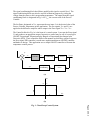
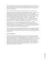
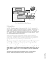
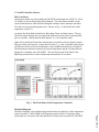
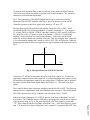
Session 3659
LabVIEW Implementation of ON/OFF Controller
Leonard Sokoloff
DeVry Institute
Abstract
This paper describes an application of LabVIEW to system control which includes data
acquisition, data processing and the display of data. The application described in this
paper emphasizes the hardware and, perhaps to a greater extent, the software used to
control a physical process. The use of the computer in data processing and control
applications is a trend that one sees in today’s industrial environment. This application is
one of many that is offered to the students in the Industrial Controls laboratory at DeVry,
in order to provide them with hands-on experience that they are likely to experience on
the job.
Virtual Instrumentation is a current technology that is making a significant impact in
today’s industry, education and research. DeVry Institute selected LabVIEW as an good
representative of this technology and is using LabVIEW in its curriculum at all DeVry
campuses in the United States and Canada. This article is a result of a research project
for LabVIEW implementation into the Industrial Controls course. LabVIEW is also used
in the communication and physics courses. LabVIEW is one of many skills that the
student will need as he enters today’s highly competitive job market.
I. Introduction
LabVIEWTM (Laboratory Virtual Instrument Engineering Workbench), a product of
National InstrumentsTM, is a powerful software system that accommodates data
acquisition, instrument control, data processing and data presentation. LabVIEW which
can run on PC under Windows, Sun SPARstations as well as on Apple Macintosh
computers, uses graphical programming language (G language) departing from the
traditional high level languages such as the C language, Basic or Pascal.
All LabVIEW graphical programs, called Virtual Instruments or simply VIs, consist of a
Front Panel and a Block Diagram. Front Panel contains various controls and indicators
while the Block Diagram includes a variety of functions. The functions (icons) are wired
inside the Block Diagram where the wires represent the flow of data. The execution of a
VI is data dependant which means that a node inside the Block Diagram will execute
only if the data is available at each input terminal of that node. By contrast, the execution
of a traditional program, such as the C language program, follows the order in which the
instructions are written.
Page 4.356.1
LabVIEW incorporates data acquisition, analysis and presentation into one system. For
acquiring data and controlling instruments, LabVIEW supports IEEE-488 (GPIB) and
RS-232 protocols as well as other D/A and A/D and digital I/O interface boards. The
Analysis Library offers the user a comprehensive array of resources for signal processing,
filtering, statistical analysis, linear algebra operations and many others. LabVIEW also
supports the TCP/IP protocol for exchanging data between the server and the client.
LabVIEW v.5 also supports Active X Control allowing the user to control a Web
Browser object.
This paper describes an application of LabVIEW to system control which includes data
acquisition, data processing and the display of data. In order to perform data acquisition,
LabVIEW software (latest version is 5.1), and the DAQ board driver software (NI-DAQ)
must be installed. The DAQ (data acquisition) board must also be installed inside the
computer. The extender board that gives the user access to various pins on the DAQ
board is connected to the data acquisition board by a flexible cable.
DAQ board contains many components that are necessary for data acquisition. A typical
board has 8 analog input data channels that are multiplexed and applied to the
instrumentation amplifier. The A/D converter digitizes the analog input data. The
onboard FIFO (First In First Out) memory provides a temporary storage of data in
buffered data acquisition applications. There are also two D/A converters that convert
digital data to analog form and pass it to the analog output ports for use by external
devices.
The DAQ board used in this application is MIO-16E-10. This is a multipurpose I/O data
acquisition board with 16 analog input ports and two analog output ports. Its settling
time of 10 µ s determines its maximum sampling rate of 100 kHz. It has a 12 bit
resolution and a 10 V dynamic range.
II. System Overview
A control system consists of components and circuits that work together to maintain the
process at a desired operating point. Every home or an industrial plant has a temperature
control that maintains the temperature at the thermostat setting. In industry, a control
system may be used to regulate some aspect of production of parts or to maintain the
speed of a motor at a desired level.
Although a control system can be of open loop type, it is more common to use negative
feedback. The block diagram shown in Fig.1a illustrates the basic structure of a typical
closed loop control system. The Process represents any physical characteristic that must
be maintained at the desired operating point. In this paper, it is the temperature that is to
be maintained at the desired value.
Page 4.356.2
The purpose of feedback is to provide the actual or the current value of process variable.
In this application a solid state temperature sensor is used to monitor the temperature. It
outputs a voltage that is too small for practical purpose, typically in the millivolt range.
The signal conditioning block that follows amplifies this signal to a useful level. The
signal conditioning block may also be used for calibration purposes by scaling the
voltage from the sensor to the corresponding temperature. The output from the signal
conditioning block is designated in Fig. 1a as VPV, the current value of the Process
Variable.
The Set Point, designated as VSP, represents the user input. It is the desired value of the
Process Variable, temperature in this application. The two signals, VPV and VSP are
applied to the difference amplifier whose output is the Error signal VE = VSP - VPV.
The Controller block in Fig. 1a is the heart of a control system. It accepts the Error signal
VE and produces an appropriate output. In practice a control may be one of several types:
ON/OFF, Proportional, Proportional plus Integral or Proportional plus Integral plus
Derivative (PID). These controllers differ in the manner in which they operate or process
the Error signal. PID controller is much more sophisticated than an ON/OFF controller
and harder to design. This application uses a simple ON/OFF controller to illustrate the
temperature control process.
Diff. Amp.
+_
Ve
Controller
Vco
Signal
Conditioning
Signal
Conditioning
Vpv
Process
Actuator
Sensor
(a)
Vco
+5V (ON)
Ve
Ve(min)
0V
(OFF)
Ve(max)
(b)
Page 4.356.3
Fig. 1 Closed Loop Control System
The Controller Output is often subjected to signal conditioning in order to provide the
proper signal level or power as required by the Actuator. If the Actuator is a motor, then
the signal conditioning block may be a power amplifier that generates the appropriate
power to drive the motor.
The use of negative feedback is the key to the proper operation of a control system.
Consider the operation of the ON/OFF control system depicted in Fig. 1b. The object of
the temperature control system described in this paper is to provide air condition
(cooling) control. Suppose that the Controller is OFF (VCO = 0V), providing no cooling.
The operating point is now on the bottom part of the hysteresis curve in Fig. 1b. This
results in increasing temperature and also in increasing VPV. The Error signal VE = VSP −
VPV is decreasing since VSP does not change. VE continues to decrease until VE =
VE(MIN). At this point the controller switches ON (VCO = +5V) and drives the actuator
(fan) in this experiment) which provides cooling. The Error signal now begins to
increase because VPV is dropping. It continues to increase until VE = VE(MAX). At this
point the Controller switches OFF, shutting OFF the fan and the cycle repeats.
The difference VE(MAX) - VE(MIN) is called the dead band. It is the range of the Error
signal in which the controller is either ON or OFF. No regulation of the Process Variable
occurs inside this range. The dead band is necessary because without it the system will
oscillate constantly between ON and OFF operating states.
This article describes a prototype that mimics the operation of a large temperature control
system. A fan is used as the actuator that provides the cooling. The graphical language
of LabVIEW, to be described in the following sections, is used to implement the function
of the controller.
III. System Hardware
The data acquisition board (DAQ board) serves as the interface between the computer
and the real world as shown by a block diagram in Fig. 2. It is installed in the PC that
operates under Windows 95. In this application MIO-16E -10 board was used. Ch. 0, one
of the analog input channels, is wired to the external temperature sensor. Ch.1 is wired to
the D/A Ch.0, one of the DAC output ports, and also to the fan. Thus the current
temperature data is coming into computer via analog input Ch. 0 and the control signal
that controls the operation of the fan comes from the computer via D/A output Ch.0. In
addition, analog input Ch.1 monitors the operation of the fan as it receives the same
signal from the computer as does the fan.
Page 4.356.4
Fan
Windows 95
DAQ
Driver
LabVIEV
Software
DAQ Board
Temp
Sensor
AICh 0
AICh 1
D/A Out Ch.0
COMPUTER (PC)
Fig. 2 System Hardware Block Diagram
IV. System Software
LabVIEW offers three categories of data acquisition VIs: Easy VIs, Intermediate VIs
and Advanced VIs. Easy VIs perform most common VI operations. They are simple to
use because the configuration complexity is designed into the VI icon. These icons
usually include some of the Intermediate VIs which in turn are made up of the Advanced
VIs. Advanced VIs are the fundamental building blocks for all data acquisition Vis and
have the most programming power and flexibility.
Analog input data acquisition options include: immediate single point input and
waveform input. In using the immediate single point input option, data is acquired one
point at a time. Software time delay to time the acquisition of the data points, which is
typically used with this option, makes this process somewhat slow.
Waveform input data acquisition is buffered and hardware timed. The timing is provided
by the hardware clock that is activated to guide the acquired data points quickly and
accurately. The acquired data is stored temporarily in the memory buffer until it is
retrieved by the data acquiring VI.
The temperature control application described in this article uses two Easy VIs. The AI
Sample Channel.vi is used to acquire data from Analog Input Channels 0 and 1 while AO
Update Channel.vi outputs 0 V or +5 V to D/A channel 0 to control the operation of the
fan.
Additional software required to run the temperature control VI described here is
LabVIEW and the DAQ board driver (NI-DAQ). These are shown in Fig. 2.
Page 4.356.5
V. On/Off Controller Software
The Front Panel
All programs which are written inside the LabVIEW environment are called VIs. Each
VI consists of a Front Panel and a Block Diagram. The Front Panel includes various
controls and indicators while the Block Diagram contains various functions and other
VIs, that are interwired among themselves. Shown in Fig. 3 is the Front Panel of the
temperature control VI.
As shown, the Front Panel includes two Waveform Charts and other objects. The top
Waveform Chart displays the error signal (the difference between the set point and the
process variable), and the bottom chart displays VCO, the Controller status.
Other objects inside the Front Panel includes the recessed box with two digital controls.
They are used by the operator to input the Set Point (VSP) value of and the scaling factor
(TCalibrate) which converts the temperature sensor output from millivolts to degrees F.
The thermometer indicator measures the current temperature and the Cooling indicator
displays the Controller state (ON orOFF). The last object in the Front Panel is the
Run/Stop switch which is used to initiate and terminate the VI execution.
Fig. 3 The Front Panel of the Temperature Controller
Page 4.356.6
The Block Diagram
The Block Diagram is the graphical program that shows the data flow of the temperature
control operation. Unlike a high level language program, like the C language where
instructions are executed in the order that they are written, the execution of a LabVIEW
VI depends solely upon the flow of data: a particular object inside the Block Diagram
will execute only if data is available or present at all its input terminals. The execution
continues at each node that has the data.
Fig. 5 shows the details of the Block Diagram which can be used to describe the
operation of the ON/OFF controller while Fig. 4 shows the hysteresis of the ON/FF
Controller operation as the Error signal varies between –2oF and +2oF.
The operation begins with a check on whether the Controller is ON or OFF. This is
accomplished with VI 2 (AI Sample Channel.vi) and the comparator C1. The output of
C1 is either TRUE or FALSE. If TRUE, then the Controller is OFF, and if FALSE then
the Controller is ON. VI 2 takes its input from Channel 1 of Device 1 (DAQ Board
number). As described earlier, analog input Channel 1 is physically wired to DAC
output Ch. 0 which controls the operation of the fan. Thus by testing the DAC output Ch.
0, we can determine whether the Controller is ON or OFF. This will place the Controller
operating point either on the lower segment or the upper segment of the hysteresis loop in
Fig. 4.
Vco
+5V (ON)
Ve
-2
0V
(OFF)
+2
Fig. 4 The Operation of the ON/OFF Controller
At this time V1, M1 and S1 determine the value of the Error signal (VE). V1 takes the
temperature sample from the analog input Ch. 0 to which the temperature sensor is wired.
M1 multiplies the temperature sample by the scaling factor (TCalibrate) and S1 subtracts
this value from the Front Panel digital control Set Point (VSP) . The result is the Error
signal.
The Controller has to make a decision whether to turn the fan ON or OFF. This decision
making process is implemented with nested Boolean Case structures. The reader should
follow the hysteresis loop in Fig. 4 and the code in Boolean Cases 1, 2 and 3.
Page 4.356.7
If the output from Comparator C1 is TRUE, then the True frame of Boolean Case 1will
be executed. The Controller must be OFF and its operating point is on the lower segment
of the hysteresis loop in Fig. 4. We must check next if the Error signal is greater than
–2oF. This is done inside the True frame of Boolean Case 1. If the Error signal is greater
than –2oF, then the True frame of Boolean Case 2 outputs 0V, keeping the fan OFF. But
if the error signal is equal to or less than –2oF, then the False frame of Boolean Case 2
outputs +5v to turn the fan ON.
If C1 output is FALSE, the Controller must be ON. Comparator C3 inside the False
frame of Boolean Case 1 checks the Error signal if it is less than +2oF. If TRUE, the
True frame of Boolean Case 3 outputs +5 V to keep the fan ON. And if FALSE then the
False frame of Boolean Case 3 outputs 0v thus switching the fan OFF.
This operation is inside the While Loop which is enabled by the RUN/STOP switch in
the Front Panel. As long as the switch is in the RUN position, its terminal counterpart in
the Block Diagram outputs a TRUE to the condition terminal keeping the While Loop
enabled; a FALSE disables the While Loop. As long the While Loop is enabled, the code
inside the loop is repeatedly executed. This results in acquiring a temperature sample
once a second. To stop the operation, the user must click on the RUN/STOP switch.
The two Waveform Charts in the Front Panel show the error signal and the Controller
output. The Controller switches between 0V and +5V as shown by the hysteresis loop in
Fig. 4.
The Wait Until Next ms Multiple function provides 1 s time delay between the data
points. The Waveform Charts shown in Fig. 3 are set to display 600 data samples (10
minutes of data).
Page 4.356.8
Fig. 5 The Block Diagram of ON/OFF Controller
Page 4.356.9
VI. Conclusion
This article focuses more on the control software than the hardware. The prime objective
is to provide the student with a practical application that uses a graphical language as a
design tool. Although only the cooling task is considered in this application, students are
assigned a project to complete the design and implement the heating control using the G
language.
The system described in this article is a prototype that mimics the operation of a large air
conditioning system. Within the constraints of the design and the limits of the physical
configuration, the system performed within the design limits. The dead band was set to
± 2oF which makes the Controller switch at +2oF at the upper end, and -2oF at the lower
end.
The rate of cooling achieved by this application was estimated to be approximately 1
minute to cool the air around the temperature sensor from 76 to 72oF. Its accurate
determination was not done because it depends on many factors such as the volume to be
cooled, enclosure and its insulating properties and other factors.
Bibliography
Basic Concepts of LabVIEW 4 by L. Sokoloff, Prentice Hall, 1997.
Analog and Digital Control Systems, by R. Gayakwad and L. Sokoloff, Prentice Hall, 1988.
Graphical Programming by G. W. Johnson, McGraw Hill, 1994.
LabVIEW Data Acquisition VI Reference Manual, National Instruments.
LabVIEW for Windows User Manual, National Instruments.
LabVIEW Function Reference Manual, National Instruments.
LabVIEW for Windows Tutorial, National Instruments.
LabVIEW Getting Started with LabVIEW for Windows, National Instruments.
Industrial Control Electronics by J. Webb and K. Greshock, 2nd Ed., Merrill, 1993.
Modern Industrial Electronics by T. Maloney, 3rd Ed., Prentice Hall, 1996.
Industrial Electronics by Humphries & Sheets, 2nd Ed., PWS-Kent, 1986.
Biography
Leonard Sokoloff was born in Russia and immigrated to the United States in 1950 and was awarded BSEE
degree from Stevens Institute of Technology (1959), the MS Applied Science degree from Adelphi
University (1964) and the PhDEE (candidate) from Stevens Institute of Technology. Worked in industry as
semiconductor application and circuit design engineer (1959 – 1970). For the past 28 years with DeVry
Institute, currently as senior professor, teaching associate level and bachelor level courses in advanced
mathematics and in electrical engineering. Currently involved in curriculum development projects using
Virtual Instrumentation, PLC and PLD.
Page 4.356.10
Page 4.356.11
Page 4.356.12
Page 4.356.13
Page 4.356.14
1
Page 4.356.15