Download Unimap - Sapienza

.
Unimap
a map making software
for PACS and SPIRE
DIET dept. - University of Rome ’La Sapienza’.
ASDC - Italian Space Agency.
IAPS inst. - National Institute of Astrophysic.
Issue 6.2 - Date: August 20, 2015
1
Contents
1 Introduction
4
2 Unimap input and output
5
3 Unimap pipeline
7
3.1
TOP: making the Time Ordered Pixels . . . . . . . . . . . . . . . . . . . . . . . .
8
3.2
Pre: signal pre-processing . . . . . . . . . . . . . . . . . . . . . . . . . . . . . . .
9
3.3
Glitch: glitch removal . . . . . . . . . . . . . . . . . . . . . . . . . . . . . . . . .
10
3.4
Drift: drift removal . . . . . . . . . . . . . . . . . . . . . . . . . . . . . . . . . . .
11
3.5
Noise: noise spectrum and GLS filter . . . . . . . . . . . . . . . . . . . . . . . . .
12
3.6
GLS: map making . . . . . . . . . . . . . . . . . . . . . . . . . . . . . . . . . . .
13
3.7
PGLS: post-processing of the GLS map . . . . . . . . . . . . . . . . . . . . . . .
14
3.8
WGLS: weighted post-processing of the GLS map . . . . . . . . . . . . . . . . . .
15
4 Using Unimap
16
4.1
Using Top . . . . . . . . . . . . . . . . . . . . . . . . . . . . . . . . . . . . . . . .
16
4.2
Using Pre . . . . . . . . . . . . . . . . . . . . . . . . . . . . . . . . . . . . . . . .
17
4.3
Using Glitch . . . . . . . . . . . . . . . . . . . . . . . . . . . . . . . . . . . . . . .
17
4.4
Using Drift . . . . . . . . . . . . . . . . . . . . . . . . . . . . . . . . . . . . . . .
17
4.5
Using Noise . . . . . . . . . . . . . . . . . . . . . . . . . . . . . . . . . . . . . . .
18
4.6
Using GLS
. . . . . . . . . . . . . . . . . . . . . . . . . . . . . . . . . . . . . . .
18
4.7
Using PGLS . . . . . . . . . . . . . . . . . . . . . . . . . . . . . . . . . . . . . . .
19
4.8
Using WGLS . . . . . . . . . . . . . . . . . . . . . . . . . . . . . . . . . . . . . .
19
5 Getting, installing and running Unimap
20
5.1
Getting Unimap and the MCR . . . . . . . . . . . . . . . . . . . . . . . . . . . .
20
5.2
Installation overview . . . . . . . . . . . . . . . . . . . . . . . . . . . . . . . . . .
21
5.3
Installing Matlab . . . . . . . . . . . . . . . . . . . . . . . . . . . . . . . . . . . .
21
5.4
Installing Unimap
21
. . . . . . . . . . . . . . . . . . . . . . . . . . . . . . . . . . .
2
5.5
Running Unimap . . . . . . . . . . . . . . . . . . . . . . . . . . . . . . . . . . . .
21
5.6
Making input and running Unimap from HIPE . . . . . . . . . . . . . . . . . . .
22
5.7
Performance and system requirements . . . . . . . . . . . . . . . . . . . . . . . .
22
5.8
Getting help . . . . . . . . . . . . . . . . . . . . . . . . . . . . . . . . . . . . . . .
22
5.9
Installing and running Unimap on a Mac
23
. . . . . . . . . . . . . . . . . . . . . .
6 Appendix
24
6.1
Matlab input . . . . . . . . . . . . . . . . . . . . . . . . . . . . . . . . . . . . . .
24
6.2
Fits input: UniHIPE and HIPE script . . . . . . . . . . . . . . . . . . . . . . . .
25
6.3
Fits header . . . . . . . . . . . . . . . . . . . . . . . . . . . . . . . . . . . . . . .
25
6.4
Parameters . . . . . . . . . . . . . . . . . . . . . . . . . . . . . . . . . . . . . . .
25
6.5
Output files . . . . . . . . . . . . . . . . . . . . . . . . . . . . . . . . . . . . . . .
28
3
Chapter 1
Introduction
Unimap is a data processing software for PACS and SPIRE data. It is written in Matlab and
implements a full pipeline, starting from the level 1 data of the standard pipeline and delivering
high quality final maps. Unimap is the successor of and was obtained from the Hi-Gal/RomaGal
pipeline [1]. With respect to the Hi-Gal pipeline Unimap offers some improvements: it is
automatic and it is a stand alone, portable package. Furthermore several novel processing
approaches are introduced. The full description of the Unimap signal processing can be found
in [5, 6, 7].
This report is a user manual for Unimap. It is a draft document. Chapter 2 gives an overview
of the I/O files and of the directory organisation. Chapter 3 illustrates the Unimap pipeline,
giving details about the modules, their parameters and output. Chapter 4 discuss several ways
of evaluating and improving the quality of the images produced by Unimap. Chapter 5 explains
what are the Unimap versions, how to get, install and run one of the versions and how to get help
from the developers. The appendix gives a detailed description of the input data and a summary
of the program parameters and output. The Unimap release described in this document is 6.2.0.
4
Chapter 2
Unimap input and output
Two directories are needed in order to use Unimap. The first one, that will be indicated as
unimap path, is the one hosting the program files. The second one, that will be indicated
as data path, is the one hosting the I/O files.
The unimap path also hosts a file named
unimap par.txt which is an ASCII file that stores the program parameters and that can be
modified with any text editor to customise the program functions. The unimap data may also
host a file named unimap header.txt which is an ASCII file that stores additional entries for
the fits header (see the appendix for a better description).
The input data must be stored in the data path before the program execution. This folder
is also used as the output folder by Unimap. The main input to Unimap is a set of bolometer
readouts and pointing information. These data can be represented by three matrices: Φ =
{φk,n }, A = {αk,n } and ∆ = {δk,n } giving, respectively, the readout, the right ascension and
the declination of the k-th bolometer at the n-th sampling instant. Additionally, a flag matrix
Fb = {fk,n }, such that fk,n = 1 is the readout is bad and fk,n = 0 otherwise, must be passed to
Unimap.
The input data for Unimap can be stored in two types of files: fits (.fits) or matlab (.mat).
The two types can be mixed. Specifically the input data is stored in files named unimap obsid ∗
.f its or unimap obsid ∗ .mat and these files have to be stored in the data path: they are
recognised and processed. Each of these files must contain the matrices Φ, A, ∆ and Fb for
some observation id. Any number of observations (within the memory limit) can be processed:
this means that Unimap can produce wide patches, involving several observations, and maps for
tiles with as many passes as desired. A description of the file formats is given in the appendix.
The file unimap par.txt stores the program parameters. When the program starts, if this file
is not found, a default copy is written in the unimap path which can next be edited by the user.
While Unimap recognises the parameters by their position in the file, for the user’s convenience
in the default file the parameter values are followed by a comment (starting with a % symbol)
the first field of which is a mnemonic name, that will be used in the following to identify the
5
parameter. For example the second line of the parameter file looks as follows
home/data/L048 psw/ % data path - working directory
and it defines a parameter, named data path, giving the I/O directory and the value of which
is home/data/L048 psw/. The parameters can be classified into two types: global and local.
Global parameters affect the whole program execution and are used by several processing steps
(modules). Local parameters only affect the functioning of one processing step (module). In the
par file, the global parameters appear first and are followed by the local parameters, grouped
by owning module. Each parameter will be better discussed in the next sections. A summary
of the parameters can be found in the appendix.
Unimap produces several output files. These can be grouped into four classes. Maps: these
are fits files, containing various versions of the final map. These files are always produced. TOP:
these are matlab files, containing various versions of input data, after the different processing
modules. They are huge files and do not really need to be saved because Unimap can store them
in RAM to speed up the execution. However, if they are saved, the execution can be repeated
starting from any module and not necessariliy from the first one. Whether they are saved of
not is controlled by the parameter run mode (see later). Work data: these are matlab files,
containing various ancillary data, that Unimap needs. These are always saved and the user has
no control on them. Evaluation data: these are fits files, containing various images that are
useful to evaluate the maps and the processing. These are useful files but not really needed
and their production can be suppressed. Whether they are saved of not is controlled by the
parameter save eval data (1 saves, zero does not). The output files will be better described in
the next sections. A summary can be found in the appendix.
The maps produced by Unimap are affected by an unknown offset and need to be calibrated
using an external, absolute reference to obtain the actual flux. This is because the PACS and
SPIRE timelines are affected by an unknown offset that cannot be estimated based on the data.
Concerning the unit of measure, Unimap follows the Hi-Gal assumptions. Namely it assumes
that the input data are MJy/sr for PACS and Jy/beam for SPIRE1 . The user can select the
output map to be in MJy/sr or in Jy/pixel.
Concerning the coordinate systems, Unimap assumes that the input pointing information is
given in equatorial coordinates. The output can be produced either in equatorial or galactic
coordinates.
At each execution Unimap saves in the data path a copy of the parameter file and a file
named unimap log.txt where the program text output is saved. By default the log file is opened
in append mode, i.e. the new output is added to the previous output. However if the parameter
start module is set to zero, the log file is cleared and previous output deleted.
1
Obviously, if the input data have a different unit, the Unimap output unit will be scaled by a multiplicative
factor.
6
Chapter 3
Unimap pipeline
In the following subsections we describe the Unimap pipeline steps, in the order in which they
are performed. We start by describing the global parameters meaning. To this end note that
each step is performed by a module and that the modules are numbered from 1 to 8. Note
that not all the steps need to be always performed; instead the user can specify a start module,
where the processing will start, and a stop module, which will be the last executed. The start
and stop module are specified by means of the parameters start module and stop module. If
the start and stop module are, respectively, 1 and 8 the whole pipeline is executed. If the start
module is zero, the log file is cleared and the program executed from module 1. By setting
these parameters equal, a single module can be executed. Note that, in order to execute an
intermediate step, all the preceding steps must have been executed in a preceding run and their
output saved (by setting to 1 or 3 the parameter run mode).
The run mode parameter determines which run mode Unimap should use. If 0, disk use is
minimised and speed is maximised; if 1, disk is maximised but step by step execution is allowed;
if 2, memory use is minimised, at the expense of some disk space; if 3, memory is minimised and
disk is maximised (to allow step by step).
Some of the modules (TOP, glitch) check whether a timeline is too flagged and discard
the data if this is true. There is a global parameter, max bad, which specifies the maximum
percentage of flagged readouts that a timeline can have to be kept in the processing.
Some of the modules (Noise, PGLS,WGLS) perform a morphological analysis of the image
in order to tune the processing. In the analysis the image is partitioned into three sets: border
(outer pixels, usually noisy and not reliable), background (inner pixels with a weak emission)
and signal (inner pixels with a strong emission). There is a global parameter controlling this
process, morpho sig thresh, which is the threshold used to detect the signal (higher means less
signal, lower more signal).
Some of the modules (drift, GLS and PGLS) perform an iterative processing. There is a
global limit to the number of iterations that can be performed which is stored in the parameter
7
max ite par.
3.1
TOP: making the Time Ordered Pixels
This module opens all the input files, which can be several, and merges the input data to form
the following three matrices: Φ = {φk,n }, A = {αk,n } and ∆ = {δk,n } containing, respectively,
the readout, the right ascension and the declination of the k-th bolometer at the n-th sampling
instant. Additionally, a flag matrix Fb = {fk,n }, such that fk,n = 1 is the readout is bad and
fk,n = 0 otherwise, is formed by this module. The matrix Fb is saved into file f lag base.mat for
inspection and for use by the subsequent modules.
The module can filter out bolometers that are too bad. To this end the parameter max bad
is used, which is a number in the range 0 to 100 giving the maximum percent of flagged data
that a timeline can have to be accepted for processing. If a bolometer exceeds this threshold it
is discarded and not used to construct the map.
The module can discard initial samples from the timelines, which can be useful to remove
an initial deviation from the baseline, affecting some dataset and due to the memory of the
calibration phase. To this end the parameter top skip exists, which is the number of initial
samples to skip. This is normally useful for PACS only and therefore the skip is suppressed for
SPIRE data. However if top skip is negative, it apllies to SPIRE too and −top skip samples
are skipped. Moreover, in order to protect short observations, no more than ten percent of the
samples are skipped, overriding the parameter value if necessary.
Unimap assumes that the input data are MJy/sr for PACS and Jy/beam for SPIRE. The
unit measure of the output is controlled by the parameter top unit. If the parameter is 0 the
output is MJy/sr. If the parameter is 1 the output is Jy/pixel. For SPIRE data, If the parameter
is 2 the output is Jy/beam.
Unimap assumes that the pointing information is given in equatorial coordinates (right ascension, declination), as is true for the standard pipeline. If requested, this module can convert
the pointing information into galactic coordinates (glon, glat), which can be useful to map the
Galaxy. This is controlled by the parameter top use galactic (1 convert, 0 do not convert).
As the next step the module projects the polar (equatorial or galactic) coordinates onto
a plane. Currently there are three possible projections implemented: gnomonic (TAN), cylindric equal area (CEA) and plate carree (CAR). The projection is controlled by the parameter
top use gnomonic (0 = CAR, 1=TAN, 2=CEA).
After projecting, the module makes a pixel grid on the projection plan, with a pixel edge that
can be specified by the user by means of the parameter top pixel size (arcsec). If this parameter
is set to zero, default values (Hi-gal) are used. It then assign numbers to all the pixels of the
grid and next assigns each readout to one of the pixel, based on the pointing information. The
8
result is a matrix P = {pk,n } giving the number of the pixel where the n-th readout of the k-th
bolometer falls. The matrices Φ and P are referred as a TOP (Time Ordered Pixels) and are
saved in the files top base.mat and poi.mat, since they are needed by the following modules.
The pixelisation can be controlled to some extent by the user. The user can specify the
dimensions of the final map, by means of the parameters top nax1 and top nax2. If top nax1
is set to zero then the dimension is automatic. The user can specify a reference point in the
projection plane, which is also used as the projection center, by means of the parameters top cva1
and top cva2 (degrees). If the first parameter is set to ’Inf’, the reference point is set to the map
center. The user can select the position of the reference point in the final map, by means of
the parameters top cpi1 and top cpi2 (pixels). If the first parameter is set to ’Inf’, the reference
point is positioned in the matrix center.
For huge maps it can be useful to run fast tests, where some of the input data is neglected
in order to speed up the processing. To this end the module may subsample the bolometers
and produce reduced output for the following modules. This is controlled by the parameter
top bolo sub, which tells this module to retain only one bolometer out of every top bolo sub
bolometers. Therefore if this parameter is one, no subsampling occurs, if it is two, half of the
bolometers timelines are dropped and so on.
As a last step, the matrix Φ is modified by subtracting the median to each timeline and the
result is saved again in the matrix Φ. If save eval data is one, the module makes a projection
of the Φ matrix at this stage and saves it in the file top base.f its; the standard deviation of
the readouts falling into each pixel is saved in top base noise.f its. The module also counts the
number of readouts per pixel and saves the corresponding image in cove f ull.f its. Moreover,
it save an image f lag base.f its where each pixel’s value gives the number of flagged readouts
falling in the pixel. This module also computes ancillary data (like the instrument type, the
scan angles etc) that are saved into the file data base.mat.
3.2
Pre: signal pre-processing
As a first step the module fixes the flagged readouts (base flags) by means of a linear interpolation
between the preceding and following valid readuts. Next, if requested by the user, the module
tries to detect the presence of calibration blocks. Calibration blocks are segments of artificial
readouts inserted into the timeline (e.g. in tile Hi-GAL L030, L059) during the turnaround
period (i.e. when the scan direction is changed) and need to be eliminated from the matrix Φ.
This step is controlled by the parameter pre cal: when the parameter is zero the detection is
suppressed. If the parameter is Inf it is assumed that the cal blocks have been flagged in the
input data; this feature will be active in HIPE 14 but if the input data have been produced with
HIPE 13.0 or lower the cal blocks are not flagged. Therefore the module has a built in detection
9
procedure that checks the lengths of the turnaround sequences and looks for longer sequences,
which are candidate to host a cal block. Specifically the module finds the median length of
the turnaround sequences and then finds sequences having a length larger than pre cal times
the median length. These sequences are candidate to host a cal bolck. Afterwards, the power
(mean squar value) of each candidate is checked and compared with the minimum power of all
turnaround sequences: if the power is greater than pre cal thresh times the min power, the cal
block is confirmed and the whole turnaround sequence hosting it is flagged. If pre cal thresh is
zero, all candidates are confirmed.
The next task of the module is to detect signal jumps (hot cold bolometers). This is done
by dividing each timeline into blocks of 2 pre jump hf win samples, computing the median and
detecting median jumps exceeding pre jump threshold times the timeline standard deviation.
When the threshold is exceeded a candidate jump is found which undergoes a set of morphological rules aiming at removing false candidates. If the candidate is confirmed, a sequence
pre jump len samples is flagged starting from the candidate. If the threshold is set to zero, the
jump detection is skipped.
As the next step the module merges (by means of a logical or) the (possible) calibration
blocks flags and signal jump flags and the result is saved into file f lag pre.mat. Optionally, a
file f lag pre.f its can be saved which is an image where the number of flagged (cal and jump)
readouts for each pixel is shown.
The module also produce a segmentation of the timelines, which is needed by GLS. Specifically each timeline is broken into segments in correspondence to any cal block or jump identified.
Moreover, also long sequences of base flags can be broken. This is controlled by the parameter
pre sat: specifically, the timeline is broken in correspondence of all sequences of base flags longer
than pre sat.
Finally the module fixes the flagged data (cal and jump). Specifically the flagged readouts
are replaced with a linear segment joining the good data and the result is still stored in the
matrix Φ. This matrix is then saved into file top pre.mat. Optionally the module can also
create an image obtained by rebinning the Φ matrix and save the image in the file top pre.f its
(the standard deviation of the rebin is also saved in the file top pre noise.f its).
3.3
Glitch: glitch removal
This module searches glitches. The first step of this module if to high-pass filter each bolometer
timeline (each row of the Φ matrix) with a non-linear, median, filter. In this way a high-pass
filtered TOP is obtained, which is stored in a matrix H = {hk,n }. The window length of
the median filter is controlled by the user by means of the parameter glitch hf win, giving, in
samples, the half window length.
10
It next performs the glitch search on the high-pass filtered top H. Glitches are detected by
observing all the readouts falling into a pixel and marking as glitches all the outliers. Specifically
the mean and standard deviation of the readouts falling in the pixel are computed and all the
readouts having a difference with the mean larger than a user definable threshold are declared
a glitch (i.e. we use sigma-clipping). The threshold is controlled by means of the parameter
glitch max dev. If this parameter is zero a default threshold is used, if it is −1 deglitching is
switched off and skipped, otherwise the parameter gives the threshold value. A lower thresold
would result into more glitches detected. The module creates a matrix of flags where an element is one if a glitch was detected and zero otherwise. This matrix is saved into the file
f lag glitch.mat. Optionally, a file f lag glitch.f its can be saved which is an image where the
number of flagged readouts (glitches) for each pixel is shown.
Next the module repairs the TOP by replacing each detected glitch with a linear interpolation
between the preceding and following good readouts. Moreover timelines with more than max bad
percent of the readouts flagged are entirelly discarded. The repaired TOP is stored in the matrix
Φ and the matrix is saved into file top glitch.mat. Optionally the module can also create an
image obtained by rebinning the Φ matrix and save the image in the file top glitch.f its (the
standard deviation of the rebin is also saved in the file top glitch noise.f its).
Note that for the glitch detection to work well, it has to be guaranteed that a sufficient
number of readouts (say 50) fall into each pixel, otherwise the outliers detection is not accurate.
However it may happen that fewer readouts than needed fall into the pixels, for example in the
Hi-GAL SPIRE maps. In this case it is necessary to subsample the image before performing
the glitch detection, in order to increase the pixel size and the number of readouts falling into
a pixel. This can be done by means of the parameter glitch sub which is a positive integer
specifying the subsampling. If it is one, no subsampling takes place. If it is two, the glitch
search is carried out on a map with pixels having half the length (one fourth the area) of the
original map. And so on. If the parameter is set to zero, the subsampling level is computed
automatically, in order to guarantee that an average of 50 redaouts fall into each pixel after the
subsampling.
3.4
Drift: drift removal
If calibration blocks have been detected, this module tries to compensate the effects of the blocks.
To this end, the timelines of each observation where cal blocks have been detected are broken
into segments in correspondance to the identified cal blocks and a (single) straitght line is fit to
the segments of (all) the timelines. The timelines are next updated by subtracting the fit. The
cal blocks compensation can be suppressed using the parameter drif t each bolo, setting it to 2
or 3 (see later).
11
Next, this module removes the drift affecting the timelines by fitting a polynomial to the
timeline. The fit procedure is better described in [6] and is based on an iterative approach.
At each iteration a better fit is obtained and the number of iterations can be controlled by
means of the parameter drif t min delta which is a positive real number giving the minimum
improvement of the Mean Square Error (MSE) (in dB and with respect to the previous iteration)
needed in order to continue the iterations. Another important parameter is the polynomial order,
controlled by the parameter drif t poly order, which is a positive integer.
After estimating the polynomial, the fit is subtracted from the original timelines of the matrix
Φ and the result still store in that matrix. The dedrifted Φ matrix is saved into file top drif t.mat.
Optionally the module can also create an image obtained by rebinning the Φ matrix and save
the image in the file top drif t.f its (the standard deviation of the rebin is also saved in the file
top drif t noise.f its). Also some ancillary data are saved into file data drif t.mat.
Note that the module can work in two different ways: either it computes a fit for each
individual timeline or it computes a single fit for all the bolometers belonging to a subarray
(recall that the PACS blue bolos are organised into 8 subarrays, PACS red into two subarrays
while SPIRE bolos all belong to the same subarray). Therefore, when the fit is carried out by
subarray only an average polynomial fit is computed, which is then subtracted to all the timelines
of the same subarray. Working by subarray is faster but may slow down the convergence of GLS.
Whether the procedure has to be carried out for each bolo or for the whole subarray is decided by
the parameter drif t each bolo: if this parameter is 1 or 3, each bolo is dedrifted separately; if it
is 0 or 2 the fit is carried out by subarray; if the parameter is 2 or 3 the cal blocks compensation
is suppressed; if this parameter is -1, the whole drift module is suppressed (as can be useful to
save computation time in images with low drift).
3.5
Noise: noise spectrum and GLS filter
As a first step this module estimates the noise spectrum and constructs the noise filters to be
used by the GLS map maker. The GLS implementation used by Unimap controls the filter len
explicitely, by means of the parameter noise f ilter hf len, which is a positive integer giving the
response half length, in samples. Normally a few tens of samples, say 50, are sufficient to obtain
well working filters.
The GLS noise filters can be constructed in two different ways, as controlled by the parameter
noise f ilter type. If the parameter is 0 the raw filters estimated from the data are used (obtained
by inverse Fourier transforming the estimated noise spectrum). If the parameter is 1 the noise
spectrum estimated from the data is fitted with a spectrum model (1/f noise plus white noise)
and the filter response is obtained by inverse Fourier transform of the fitted spectrum. If the
parameter is set to Inf, it is reset to 1 for PACS and to zero for SPIRE. To check the filters,
12
the module saves two files: noise spec.f its, containing the estimated noise spectrum for each
bolometer, and noise f ilt.f its, containing the actual filter response used for each bolometer.
As a second step this module formats the data for the GLS step. It first load the signal jump
and the calibration block flags that were produce by the P re module and breaks the timelines
into segments, by placing a break where a jump or a cal block was found. The segments will
be handled separately, as independent timelines, in the GLS iterations. Next the module may
or not remove the flagged values, as controlled by the parameter noise apply f lag. If this
parameter is one, the flagged data will be skipped and not used during the GLS iterations. If
this parameters is zero the flagged data are replaced with the reconstructed data (obtained by
linear interpolation of the timeline) and used by the map maker.
Using the updated TOP, the module makes a projection to construct the naive map, which is
the first Unimap output, saved in the file img rebin.f its. The corresponding standard deviation
image is saved in file img noise.f its. Also a coverage image is saved, counting the valid readouts
(after flag removal), in file cove gls.f its. The module also computes the morphology of the
image, classifying each pixel into void (0), border (1), background (2) or signal(3). The process
is controlled by a global parameter: morpho sig thresh which is the threshold used to detect
the signal (higher means less signal, lower more signal). The morphology is saved in the file
f lag morpho.f its. Ancillary information is saved in f lag dive.f its, which gives a diversity score
for each pixel, counting the readouts from different bolometers.
3.6
GLS: map making
This module makes a map (image) from the timelines by exploiting a Generalised Least Square
(GLS) approach, e.g. [2]. The implementation exploits the Parallel Conjugate Gradient (PCG)
and is therefore similar to other implementations like [1, 3, 4]. However the implementation
has specific features that are better described in [7] but will not be covered in deep here. Nor
we will present a deep description of the GLS approach, which can be found in the references
just given. We will limit ourselves to a short description, useful to understand the Unimap
parameters affecting the GLS map maker.
The GLS map is obtained from the deglitched and dedrifted Φ matrix. The GLS approach
is an iterative one, where at each iteration the timelines are filtered with a noise whitening filter
and rebinned into a map. The number of iterations is controlled by means of the parameter
gls min delta as follows: at each iteration the variance of the correction applied to the map
normalised by the variance of the map is computed (in dB) and if it is lower than gls min delta
(in dB) the processing is stopped. By setting this parameter to -Inf, the number of iterations
performed will be exactly the one given by the parameter max ite par. By setting this parameter
to Inf, the stop level will be automatically selected based on the image morphology. At the end
13
of the iterations the module saves a GLS image, in the file img gls.f its. Some ancillary data are
saved into the files data gls.mat and data gls ite.mat. The module also saves a useful evaluation
image. Specifically the naive (rebin) image is subtracted from the GLS map and the result is
saved in the file delta gls rebin.f its.
The GLS needs a map to start with and there are three possible choices, as controlled by
the parameter gls start image. If this parameter is 0, the GLS will start from a zero map. If
the parameter is 1, the GLS will start from the rebinned map. If the parameter is 2, the GLS
will start from a mixture of a flat map (corresponding to the background) and the rebin (where
the signal is). If the parameter is 3, the GLS will start from the last saved GLS image and data,
which is useful to do more iterations on a previous GLS run. If the parameter is Inf, Unimap
will automatically select the start image based on the image morphology. In theory, after a
sufficent number of iterations, the GLS will converge to the same map irrespectively of the start
map. However the number of iterations required to converge will vary depending of the start
map. When the image has a strong signal it is better to start from the rebin. When the signal
is weak and the sky is essentially an almost flat background with a few sources it is better to
start from the zero or the mixture map. This is the rationale applied in the automatic start
image selection, which selects rebin or mixture depending on how much signal is found.
3.7
PGLS: post-processing of the GLS map
The GLS map maker is known to introduce some artifacts and distortion in the map [5]. Therefore this module runs the PGLS algorithm [5], which is a way to (partially) remove the artifacts
and the distortion introduced by the GLS map maker, especially for PACS data. The PGLS
algorithm will not be discussed in deep here. We only mention that PGLS tries to estimate the
artifacts introduced by the GLS map maker and then subtracts the artifact estimate from the
GLS image, to produce a clean image which is saved in the file img pgls.f its. In so doing, the
PGLS algorithm may amplify the background noise of the image, so that it is not always obvious
that the PGLS image is better than the GLS one. The module also saves a useful evaluation
data that is the distortion estimate, i.e. the difference between the GLS and the PGLS map, in
the file delta gls pgls.f its. Furthermore it saves the difference between the PGLS map and the
rebinnaed image in the file delta pgls rebin.f its.
PGLS is an iterative process involving a non-linear, median high-pass filter. The length of the
median filter is controlled by the parameter pgls hf win, which is a positive integer specifying
half of the filter length. Higher lens improve the artifact estimation and are needed if the
artifacts are wide, but also may increase the background noise level. Lower lens reduce both the
noise and the artifact estimation quality. If the parameter is set to zero, the module attempts
to determine an optimal value. This is done by running PGLS many times and measuring the
14
distortion and may greatly increase the computation time. There are two more parameters
controlling the convergence: pgls num ite which sets the numer of iterations to be performed,
and pgls min delta, having a meaning and an effect similar to gls min delta. If these parameters
are set to zero, the values are automatically computed.
3.8
WGLS: weighted post-processing of the GLS map
Since the PGLS remove the GLS distortion but increases the background noise, it is convenient
to make a mixed map, obtained from the PGLS image only where the distortion is strong (so that
it is removed) and from the GLS image where there is no distortion (so that the background
noise is not increased). This is done in this module which runs the WGLS algorithm [5, 7].
The algorithm computes a distortion mask, having the same size of the image, which is zero
where no distortion is detected and is one where distortion is detected. Then the WGLS image
is obtained from the PGLS image where the mask is one and from the GLS image when the
mask is zero. The WGLS image is saved into file img wgls.f its and the mask used may be
saved in the file f lag wgls.f its. This module also saves a useful evaluation image. Specifically
the rebinned image is subtracted from the the WGLS image and the result is saved in the file
delta wgls rebin.f its.
The WGLS currently implemented in Unimap is the one described in [7] and creates the
distortion mask in two step. The first step creates anchor points for the distortion which are
grown in the second step. Specifically, in the first step the distortion image produced by the
PGLS is compared with a threshold, specified by the parameter wgls dthresh, and all the pixels
with a difference from the mean greater than the standard deviation times the threshold are
declared as distortion pixels and set to one in the WGLS mask. In the second step the distortion
image is compared with a threshold, specified by the parameter wgls gthresh, and all the pixels
with a difference from the mean greater than the standard deviation times the threshold and
adiacent to a pixel already flagged are declared as distortion pixels and are set to one in the
WGLS mask. The second step is repeated until no more pixels are added to the mask. If either
parameter is set to zero, its value is computed automatically.
15
Chapter 4
Using Unimap
Using the default parameters a decent image will be obtained for most of the PACS and SPIRE
observations. In this sense Unimap is an automatic map maker. However the image quality
needs to be checked and often it can be improved by tuning the parameters to the specific
observation. The parameter tuning is carried out by means of a trial and error approach, where
the user attempts to vary the parameters in order to improve the quality, and judges the results
based on the evaluation data saved by the program. In this sense Unimap is an interactive map
maker.
In this section we discuss the parameter optimization and how to evaluate the map quality
based on the evaluation data saved by Unimap. We also describe some known problems that
can arise and the way to mitigate them. The results reported in this chapter ar mainly based
on the reduction of PACS data. SPIRE data will be better investigated in the future.
As a general comment, observations which are large and signal rich (e.g. a Hi-GAL Galaxy
tile) are simpler and faster to process. The default parameters are optimised for the latter case
and the Unimap output is normally high quality. On the contrary when the observation is short
or it is signal poor (e.g. a small target embedded in a flat, void background) the processing is
more difficult and some trials are needed to obtain good maps. Also note that if the data is not
redundant (at least two passes with different scan orientation) the map quality will not be good.
4.1
Using Top
Keep an eye on the text outupt of the module. Check if too many bolometers are discarded,
and increase the top max bad value in this case.
Have a look to top base.f its and top base noise.f its to see if there is impact of the inital
calibration phase, seen as an area with high noise at the beginning of the scan. Increase top skip
if necessary.
The module prints the percentage of flagged readouts. A sane percentage is well below 1%.
16
If the percentage is much higher, the input data is not good. Have a look to f laf base.f its to
see where the flagged data are.
4.2
Using Pre
Check the impact of the jump and cal blocks detection by inspecting f lag pre.f its. Also check
the top pre.f its map and the corresponding noise. Compare with top base.f its.
Keep an eye on the text output: if cal blocks were found, check whether this is correct or
not. In case modify pre cal.
The module prints (on the screen and in the log file) the percentage of readouts that were
flagged because recognised as jumps or saturated pixels. A sane percentage is well below 1%,
a typical percentage being 0.2%. If the percentage is much higher, you should adjust the jump
threshold to lower it! The module also prints the average number of segments per timeline.
Unless cal blcks were found, this number should be very close to 1.
4.3
Using Glitch
The glitch procedure normally works well with the default values (i.e. automatic subsample and
threshold). Check the impact of the glitch removal by inspecting the f lag glitch.f its image and
by comparing the top glitch.f its (and noise) with the top pre.f its.
The module prints (on the screen and in the log file) the percentage of readouts that were
flagged because recognised as glitches. A sane percentage is well below 1%, a typical percentage
being 0.2%. If the percentage is much higher, you should adjust the glitch threshold to lower it!
4.4
Using Drift
The default polinomial order, 2, is often a good choice, but for some images different values
may yield better results. Moreover, especially when the scan is short, the drift may be small.
In this case it may be better to entirelly skip the dedrift and leave the task to the GLS map
maker. Inspect the top pre.f its to decide if the dedrifting is needed and the polynomial order.
Compare top pre.f its with top drif t.f its to asses the results of the dedrifting step.
Dedrifting by bolometer is the default choice and it is normally ok: it produces better naive
maps than dedrifting by subarray. However it may occasionally introduce bowls around strong
sources (well, very strong sources). In this case use dedrift by subarray: the naive maps may be
more moisy but the GLS should be able to produce a good estimate in any case.
If you are making a patch using several partially overlapping observations, the different
observations may have a visibly different level in the top drif t.f its map. If this is the case, GLS
17
will have problems. This can usually be corrected by increasing the numbr of drift iterations,
by lowering the parameter drif t min delta.
4.5
Using Noise
The noise filters are obtained by IFT of the noise spectrum. In the IFT, the user can decide to use
the raw spectrum (filter types 0,2) or a fit (filter types 1,3) to the spectrum. In general fitted
filters yield smoother responses and improved numerical stability in the GLS step. However
wihich filter to use also depends on how well the fit model (1/f plus white noise) follows the raw
spectrum. We found that for PACS and SPIRE PSW the fit is a good model while for SPIRE
PMW and PLW the spectrum tends to rise at the high frequencies and the fit model is no more
good. Inspect the noise spec.f its file to check the raw spectrum.
The filter response should peak in the center and drop towards zero at the extremes. Inspect
the noise f ilt.f its file to observe the filter responses. If the reponse does not reach zero (well,
small values) you may increase the filter len. To be sure that the filter len is correct, you may
make a reduction with a double filter len and check that the results are unchanged.
Have a look to the image morphology in f lag morpho.f its: this affects several following
steps. If this is badly wrong, play with the parameter morpho sig thresh to fix it.
Concerning the flags, the best option is to remove them (noise apply f lag = 1), since in this
way no artificial data are injected in the map. However removing the flags may cause instabilities
in the GLS iterations and void pixels (NaN) in the final map. In this case you can try to use
the reconstructed values.
4.6
Using GLS
The Unimap implementation of the GLS map maker is normally safe but it can sometime become
unstable. In this case you have to change the previous steps (e.g. improve dedrift or the filter
type and len). During the iterations the GLS module prints the the Delta (variance of the
correction over variance of the map). In a stable iteration the Delta should have an decreasing
trend. Small variations from the trends are ok but long or large variations from the trends
indicate that the algorithm has become unstable.
The number of iterations required to converge depends of the observation type. If it is signal
rich, a few tens of iterations are enough. If it is dominated by the noise, hundreds of iterations
may be required.
Concerning the start image, note that, in theory, the GLS should arrive at the same map
independently of the start image. Therefore when the maps obtained starting from different
images are identical, this is a safe indication that convergence was achieved. In practice, real
18
convergence is difficult to obtain due to numerical noise (round offs): it may take too many
iterations to really obtain the same map. In this case one has to choose which image is better
to start with.
The selection of the start image depends on the observation. If the observation is signal
rich (e.g. the Galaxy), then it is better to start from the rebin. When the observation is a flat
background with a few sources, both start maps (zero and rebin) should be considered. Indeed
starting from the rebin may cause disuniformities in the background, which is not flat, but has
wide stripes of different level. Instead, starting from the zero image normally guarantees a flat
background but introduces black wide holes centered around the sources. Both problems tend to
disappear by doing more iterations, but by selecting the proper start image one may significantly
reduce the number of iterations required to obtain a satisfying map.
4.7
Using PGLS
PGLS is not always necessary, because in some cases (e.g. images dominated by the noise) the
GLS algorithm does not really introduces distortion. In order to decide if PGLS is to use and
to evaluate the results, a set of delta images is produced by Unimap.
The first is delta gls rebin.f its which is the difference between the GLS image and the rebin.
This image will contain the 1/f noise (which is removed by the GLS but not by the rebin) plus
the GLS distortion and residual white noise. Check this map and if you see only 1/f noise (i.e.
stripes following the scan lines) then probably PGLS is useless. On the contrary if you see signal
related structures in the image (anything different from 1/f and residual white noise), this is the
GLS distortion and PGLS will be useful.
The second is delta gls pgls.f its which is the difference between the GLS image and the
PGLS one and is theferore the distortion estimated by the PGLS. This image shall contain the
GLS distortion observed in the delta gls rebin.f its and residual noise. Finally you should check
delta pgls rebin.f its which is the difference between the PGLS image and the rebin. This image
shall contain only the 1/f noise and residual white noise. If you still see signal related structures
in this image, then PGLS was not able to remove all the distortion. In this case it is a good
idea to increase the length of the PGLS filter: in this way the distortion estimation is improved
at the cost of some additional noise. Doing more than 4 iterations is normally useless.
4.8
Using WGLS
Inspect the f lag wgls.f its and delta wgls rebin.f its images to evaluate the results. Change
the WGLS thresholds if results are not satisfactory.
19
Chapter 5
Getting, installing and running
Unimap
Unimap can be used as a stand alone program or as a HIPE plug-in. In particular, starting from
HIPE 13, there is a HIPE script which is maintained by the PACS ICC and that can be used
to run Unimap directly from HIPE. See the HIPE documentation. In the following we discuss
the stand-alone option, focusing on the Linux case.
Unimap is written in Matlab and can run on any computer where Matlab can be installed
(including Windows, Linux and MAC). Furthermore the program can be compiled an run also
without installing Matlab: it suffices to install the Matlab Runtime Runtime (MCR).
If Matlab is installed you can use the Unimap source code directly (the source code of Unimap
5.5.0 is allowable on the page under an open source licese for you to play with and modify).
If Matlab is not installed you have to follow an installation procedure which varies depending
on the operating system. In the following we report the steps to follow to install Unimap on a
PC with Linux (specifically we tested the steps with Ubuntu 11.0.4 and 14.04 64bit and with
Debian 7.8).
5.1
Getting Unimap and the MCR
Unimap can be downloaded from http://infocom.uniroma1.it/unimap. For Linux, it comprises
the following three files:
run unimap.sh - shell for launching unimap
unimap - unimap executable
unimap par.txt - unimap default params
Additionally you have to download the MCR installer (M CRInstaller.bin): for MAC, this
is found on the Unimap page; for Linux, and starting from Unimap 6.0, you have to download
it from the Mathworks site. Select MCR version 8.4 for Matlab 2014b, 64 bit machine.
20
5.2
Installation overview
The installation is divided into two steps: installing MCR and installing Unimap. If the PC
already has (the correct) MCR installed, the first step can be skipped, but the path of the MCR
must be identified.
5.3
Installing Matlab
In order to install the Matlab Compiler Runtime (MCR) library we took the following steps
1) Copy M CRInstaller.bin to a working directory on the target PC.
2) Edit the file rights of M CRInstaller.bin: make it executable (chmod 777 M CRInstaller.bin).
3) From a terminal window, launch M CRInstaller.bin. (./M CRInstaller.bin or, if there
are writing problems, sudo./M CRInstaller.bin).
At this point the Matlab runtime library installation wizard will start and install matlab. It
will tell you what is the path to use to reach the library. It is something like /opt/M AT LAB/
M AT LAB Compiler Runtime/v84/. This path will be referred as M CR path.
5.4
Installing Unimap
Installing Unimap simply requires copying into any folder the following three files: run unimap.sh,
unimap and unimap par.txt. The folder will be termed the unimap path.
Next you have to change the mode of the run unimap.sh and unimap files and make them
executable (chmod 777 ...).
5.5
Running Unimap
Set up a data folder (data path, must be different from unimap path) and copy there the input
data: the input data are files of the form unimap obsid ∗ .f its or unimap obsid ∗ .mat. Next
section explains how to produce them.
Edit the unimap par.txt file. Write the data path as first parameter and modify the other
parameters according to your preferences.
Run Unimap by opening a terminal window, cding to unimap path and issuing the following command ./run unimap.sh M CR path where M CR path is the path where Matlab
is installed on the PC. If the data path requires privileged access you may need to issue
sudo./run unimap.sh M CR path.
21
5.6
Making input and running Unimap from HIPE
In order to use Unimap you have to build the input files. One option is to do this by yourself
(writing a wrapper producing either the .fits of the .mat input for unimap).
For PACS data, a second option is to use a HIPE script (available from HIPE 13 on) that
produces the input and runs Unimap directly from the HIPE environment. This is the recommended way of producing inputs, because the script is maintained by the ICC and wil use the
best calibration options for Unimap. The script can also be used to produce the input only; next
you can use the stand-alone Unimap, running it from outside HIPE on the input just produced:
when the data set is huge, this is a better option, because takes less memory.
A third option, suitable for both SPIRE and PACS data, is to use a HIPE user-contributed
script, named UniHIPE, that has been written by the ASI Science Data Center (ASDC). The
script can be downloaded directly from the ASDC page or accessed as a HIPE plug-in. Also
UniHIPE can be used to run Unimap within HIPE or just to produce the input files for the
stand-alone Unimap version.
5.7
Performance and system requirements
The system parameter mainly affecting the Unimap performance is the RAM. The more RAM
there is, the bigger the images that can be produced and the faster the production. To give
an idea let us say that on a laptop with 8 Giga RAM, a single Hi-GAL blue tile (nominal and
orthogonal scans) is processed in half hour. From Unimap 6, an estimate of the RAM required
is as follows: if the data have N readouts in total, unimap take about 16N bytes.
The running time varies approximately linearly with the size of the input. However if the
input size grows too big to fit into the RAM, the execution time will increase sharply due to the
need of making disk access. For example processing two Hi-GAL blue tile takes more than five
hours on the 8 Giga laptop, due to the disk access.
When the input size grows beyond a limit, the operating system cannot allocate the memory
and the program stops with an error.
5.8
Getting help
If you have problems with Unimap write an email to [email protected]. Attach the
unimap log.txt and unimap par.txt files to the email.
22
5.9
Installing and running Unimap on a Mac
The installation package and procedure for a Mac are almost identical to those described for
Linux. In the following we summarise the steps we took for a succesfull installation:
1) uncompress the Unimap package into a working directory. Rename the file readme.txt (it
contains some Matlab generated suggestions) to readme unimap.txt.
2) unzip the MCRInstaller and install it by starting the program in
/InstallF orM acOSX.app/Contents/M acOS (InstallForMacOSX). This will probably install
the MCR in a directory called
/Applications/M AT LAB/M AT LAB Compiler Runtime/... make sure that you have the version v716!
3) create a new directory where you wish to reduce your data
(e.g. /home/mycomputer/mymaps/) and where you will download your data
(e.g. /home/mycomputer/mymaps/Data/). cd /home/mycomputer/mymaps/
4) copy from the working directory the files run unimap.sh and unimap par.txt and the entire
directory unimap.app in /home/mycomputer/mymaps/.
5) transfer all data you wish to map into the /home/mycomputer/mymaps/Data/ directory
6) edit the unimap par.txt file according to your needs (especially the path of the data, first
line: in our case:
/home/mycomputer/mymaps/Data/)
7) If required, edit the script runu nimap.sh : write the correct path to the unimap program in
the exe dir variable (line 8)
(e.g. unimap.app/Contents/M acOS/)
8) run unimap by typing :
./run unimap.sh/Applications/M AT LAB/M AT LAB Compiler Runtime/v716/
23
Chapter 6
Appendix
6.1
Matlab input
Unimap will process all Matlab files named unimap obsid ∗ .mat that it finds in the working
directory. A Matlab file is a collection of Matlab variables, that are loaded into the memory by
loading the file. Specifically a input for Unimap must contain the following variables:
val. This is a Nb by Nd matrix, where Nb is the number of bolometers stored in the matlab
file and Nd the number of readouts stored for each bolometer. val(k, n) is the n-th readout of
the k-th bolometer.
ra. This is a Nb by Nd matrix. ra(k, n) is the right ascension of the n-th readout of the k-th
bolometer (in degrees).
dec. This is a Nb by Nd matrix. dec(k, n) is the declination of the n-th readout of the k-th
bolometer (in degrees).
fla. This is a Nb by Nd matrix. f la(k, n) is one (true) if the n-th readout of the k-th
bolometer is saturated or corrupted, it is zero if the readout is good.
bno. This is a Nb by 1 vector. It gives the number (i.e. the position in the instrument grid)
of the k-th bolometer. For example PACS has 2048 bolometers, numbered from 1 to 2048, but
not all these bolometers need to be passed to Unimap (for example many are bad bolometers)
so that Nb may be less than 2048. bno(k) must contain the number of the k-th bolometer stored
in the Matlab file.
scn. This is a Nd by 1 vector. It gives the scan leg to which the readout belongs. The PACS
and SPIRE observations are typically carried out along several scan legs (line of observations)
which are numbered from 1 to the number of scan legs. scn(n) = j means that the n-th readouts
(of all the bolometers) has been taken along the j-th scan leg. scn(n) = 0 means that the n-th
readouts (of all the bolometers) has been taken during a turnaround (passing from one scan
leg to another one). scn(n) = −1 means that the n-th readouts (of all the bolometers) host a
calibration block and should be flagged.
24
ist. This is a scalar specifying the instrument. Value 2048 means the instrument is PACS
blue, 512 is PACS red, 144 is SPIRE PSW, 93 is SPIRE PMW and 48 is SPIRE PLW.
6.2
Fits input: UniHIPE and HIPE script
Unimap will process all files named unimap obsid ∗ .f its that it finds in the working directory.
Input data in FITS format suitable for Unimap can be produced on any machine where HIPE
is installed by means of a tool developed by the ASDC, named UniHIPE. The tool can be
downloaded, together with the documentation, from the ASDC site,
http : //herschel.asdc.asi.it/index.php?page = unimap.html or accessed as a HIPE plug-in.
The tool is also pointed from the Unimap home page. For PACS, since HIPE 13, there is HIPE
script maintained by the ICC that interfaces HIPE with Unimap.
6.3
Fits header
Unimap writes a simple header in the fits files it saves, with a few, self explanatory fields. The
header can be enriched and customised by storing a file named unimap header.txt together with
the Unimap input data. Each line of this file specifies a header keyword that will be added to
the fits header. Each line must have the following format: ’xxxxxxxx= *’, where ’xxxxxxxx’ are
8 chars giving the keyword name and ’*’ is a char value that will be added in the header.
If Unimap finds a file unimap header.txt at runtime, these data are added to the fits header.
Otherwise only the simple header is saved.
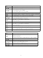
6.4
Parameters
GENERAL
data path
Name of the I/O directory (must end with a slash).
max ite par
Positive integer. Global iteration limit.
start module
Integer in [0,8]. Start module (if 0 clears the log.)
stop module
Integer in [0,8]. Last module.
max bad
In [0, 100]. Max percent of flagged samples allowed for a bolometer.
morpho sig thresh
Positive real. Threshold for signal detection in morpho analysis.
save eval data
Binary 0/1. If 1 saves evaluation data, if zero does not.
run mode
0: max speed/min disk; 1: max disk; 2: min ram; 3: min ram/max disk.
25
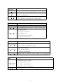
TOP
top use galactic
Binary (0/1). If 1 convert to galactic coord, if zero keep equatorial.
If 0 use no projection (CAR),
top use gnomonic
if 1 use gnomonic projection (TAN),
if 2 use cylindric equal area projection (CEA).
top bolo sub
Positive integer. Bolometers subsampling
top skip
Positive integer. Number of samples to discard at the beginning of each timeline.
top unit
If 0 output is MJy/sr. If 1 is Jy/pix. If 2 is Jy/beam (SPIRE)
top pixel size
top cva1
top cva2
top cpi1
top cpi2
top nax1
top nax2
Positive real. If 0 use the default pixel size,
otherwise this is the pixel size to use (arcsec).
Real. First coord of the map ref. point (degrees).
If Inf it is automatic.
Real. Second coord of the map reference point (degrees).
Real. First coord of the map ref. point (pixels).
If Inf it is automatic.
Real. Second coord of the map reference point (pixel).
Positive integer. Number of rows of the map.
If zero or negative the number of rows and cols is automatic.
Positive integer. Number of cols of the map.
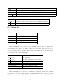
PRE
Positive real. If 0 suppress calibration blocks detection,
pre cal
if Inf use input flags
otherwise max/median len of turnarounds seqs to declare a candidate.
pre cal thresh
max/min pow of turnarounds seqs to confirm a candidate.
pre sath
min len of an input flag sequence to break into segments.
pre jump threshold
Positive real. If 0 suppress jump detection,
otherwise threshold for jump detection.
pre jump hf win
Half len of the jump search block (samples).
pre jump len
Number of samples to flag after a detected jump.
26
GLITCH
glitch hf win
Positive integer. Half len of the highpass filter (samples).
Positive integer. Subsampling for glitch search (pixels).
glitch sub
If zero it is automatic.
Positive real. Threshold to declare a readout a glitch,
glitch max dev
if zero threshold is automatic. If -1 skip deglitch.
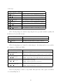
DRIFT
drif t poly order
Positive integer. Polynomial order.
drif t min delta
Real. Minimum improvement to continue iteration (dB).
If -1 skip dedrift,
if 0 dedrift by subarray,
drif t each bolo
if 1 dedrift by bolo
if 2 by subarray no cal blocks
if 3 by bolo no cal blocks.
Noise
If 0 use reconstructed values,
noise apply f lag
if 1 don’t use the flagged readouts.
If 0 use raw filters,
noise f ilter type
if 1 use fitted filters
if Inf set automatically.
noise f ilter hf len
Positive integer. Half len of the noise filter response (samples).
GLS
If 0 start from a zero image,
gls start image
if 1 start from the rebin
if 2 start from the mixture
if Inf select start automatically.
gls min delta
Real. Minimum variation to continue iteration (dB). Inf for auto select.
27
PGLS
pgls hf win
Positive integer. Half len of the pgls highpass filter (pixels). If 0 search for best.
pgls min delta
Real. Minimum variation to continue iteration (dB). If 0 use automatic selection.
pgls num ite
Integer. Number of iterations. If 0 select automatically.
WGLS
wgls dthresh
Positive real. Threshold to declare a readout an artifact. 0 is auto.
wgls gthresh
Positive real. Threshold to grow an artifact. 0 is auto.
6.5
Output files
• The following images are the main Unimap output.
MAPS
img rebin.f its
The naive (simple projection) map.
img gls.f its
The GLS map.
img pgls.f its
The PGLS map.
img wgls.f its
The WGLS map.
img noise.f its
The standard deviation of the naive map.
• The following images are obtained by projecting flag matrices. They are images where
each pixel has a value equal to the number of flagged readouts falling in it. Exception is the
f lag wgls.f its image that is one where WGLS detected an artifact and zero elsewhere. Other
exception is morphology (see the manual)
EVALUATION: FLAGS
f lag base.f its
The input flags.
f lag pre.f its
The PRE flags, jumps and cal blocks.
f lag glitch.f its
The Glitch flags.
f lag wgls.f its
The WGLS mask.
f lag morpho.f its
The morpho mask before GLS.
f lag dive.f its
Number of readouts from different bolos.
• The following images are obtained by rebinning (projecting) the matrix Φ after various
steps. In the projection no flags are applied. Also the standard deviation of the projection is
computed for each pixel and saved as ’noise’ image. These images are useful to check the results
28
of the steps.
EVALUATION: MAPS
top base.f its
The projection of the Φ matrix after TOP.
top base noise.f its
The standard deviation of the last projection.
top pre.f its
The projection of the Φ matrix after PRE.
top pre noise.f its
The standard deviation of the last projection.
top glitch.f its
The projection of the Φ matrix after Glitch.
top glitch noise.f its
The standard deviation of the last projection.
top drif t.f its
The projection of the Φ matrix after Drift.
top drif t noise.f its
The standard deviation of the last projection.
• The following images are useful for inspecting the noise spectrum estimation quality and
the filters used by the GLS module.
EVALUATION: NOISE
noise spec.f its
The estimated noise spectrum for each bolometer.
noise f ilt.f its
The filter response used for each bolometer.
• The following images are obtained by subtracting two other images and are very useful for
the evaluation of PGLS and WGLS.
EVALUATION: DELTA
delta gls pgls.f its
delta gls rebin.f its
delta pgls rebin.f its
delta wgls rebin.f its
GLS minus PGLS map.
This is the GLS distortion estimate made by the PGSL.
GLS minus rebin map.
Main components are the GLS distortion and 1/f noise.
PGLS minus rebin map.
Main component should be 1/f noise.
WGLS minus rebin map.
Main component should be 1/f noise.
• The following images contain coverage masks. Each pixel has a value equal to the number
of readouts falling into it.
29
EVALUATION: COVE
cove f ull.f its
The full coverage, with no flagging at all.
cove gls.f its
The GLS coverage, where the GLS flagging is considered.
• The following matlab files contain the matrix Φ after various steps and the pointing matrix.
TOP
poi.mat
The pointing matrix computed by the TOP module.
poi glitch.mat
The pointing matrix computed by the Glitch module.
poi noise.mat
The pointing matrix computed by the Noise module.
top base.mat
The Φ matrix after the TOP module.
top pre.mat
The Φ matrix after the PRE module.
top glitch.mat
The Φ matrix after the Gitch module.
top drif t.mat
The Φ matrix after the Drift module.
top noise.mat
The Φ matrix after the Noise module.
• The following matlab files are used to store flags and ancillary data.
WORK
f lag base.mat
Base flags.
f lag pre.mat
PRE (jump and cal blocks) flags.
f lag glitch.mat
Glitch flags.
data base.mat
Ancillary data from the TOP module.
data pre.mat
Ancillary data from the Pre module.
data glitch.mat
Ancillary data from the Glitch module.
data drif t.mat
Ancillary data from the Drift module.
data noise.mat
Ancillary data from the Noise module.
data gls.mat
Ancillary data from the GLS module.
data gls ite.mat
Ancillary data from the GLS module.
data pgls.mat
Ancillary data from the PGLS module.
data pgls ite.mat
Ancillary data from the PGLS module.
30
Bibliography
[1] A. Traficante et al., ”The data reduction pipeline for the Hi-GAL survey”, Monthly Notices
of the Royal Astronomical Society, Volume 416, Issue 4, pp. 2932-2943, Oct. 2011.
[2] M. Tegmark, ”How to make maps from cosmic microwave background data without losing
information”, The Astrophysical Journal, 480, pp. L87-L90, May 1997.
[3] C. M. Cantalupo, J. D. Borrill, A. H. Jaffe, T. S. Kisner, R. Stompor, ”MADmap: A
massively parallel maximum likelihood cosmic microwave background map-maker”, Astrophysical Journal, Supplement Series 187 (1), pp. 212-227, 2010.
[4] P. Natoli, G. De Gasperis, C. Gheller, N. Vittorio, ”A map-making algorithm for the Planck
surveyor”, Astronomy and Astrophysics 372 (1), pp. 346-356, 2001.
[5] L. Piazzo, D. Ikhenaode, P. Natoli, M. Pestalozzi, F. Piacentini, A. Traficante ”Artifact
Removal for GLS Map Makers by means of Post-Processing”, IEEE Trans. on Image Processing, Vol. 21, Issue 8, pp. 3687-3696, 2012.
[6] L. Piazzo, P. Panuzzo, M. Pestalozzi: ”Drift removal by means of alternating least squares
with application to Herschel data”, Signal Processing, vol. 108, pp. 430-439, 2015.
[7] L. Piazzo, L. Calzoletti, F. Faustini, M. Pestalozzi, S. Pezzuto, D. Elia, A. di Giorgio and S.
Molinari: ’Unimap: a Generalised Least Squares Map Maker for Herschel Data’, MNRAS,
2015, 447, pp. 1471-1483.
31