Download Chapter 1: The Basics

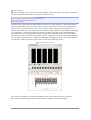
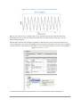
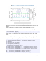
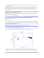
Chapter 1: The Basics
1 Introduction
This guide is an extract of a larger PACS data reduction guide that will be available by the end of the
summer, 2009. It has been provided for the Data Processing Workshop, taking place at ESAC in March,
2009. Please do not use this guide to reduce any science data you will get once Herschel has been
launched and is gathering data, because over the summer the details of the reduction of PACS data will
change, and what is here will be incomplete and may even be wrong.
On the help page, that you can access via HIPE, there are various other documents to read concerning
using HIPE and reducing and analysing data. The HowTo is particularly recommended for those starting
with HIPE for the first time. On the Help Page there is also a link to "PACS User Manual". Please be warned,
this manual has been written for use by internal PACS people, and will be very difficult for anybody else to
follow as it also concerns levels of data that you will almost never need to access. We do not recommend
you read that manual just yet.
This particular document that you are reading concerns PACS spectroscopy. For photometry other
documentation is being provided at the workshop.
Please note there is often more than one way to do something in HIPE and more that one syntax possible
within the commands. Hence, if there are differences between what is written here and the demo scripts
given out during the workshop, don't panic! The demo scripts have been written specifically for the
workshop and for the data there provided, and they should be followed first.
I would really appreciate any comments you have on this documentation. The more comments I get, the
better the final version will be! Email to Katrina Exter at [email protected].
2 PACS data structure
The PACS data structure is multi-layered and difficult to explain in a few words. Better documentation on
this is being written and will be available to you at a later date. But a quick explanation follows.
Bear in mind that during a single PACS observation you can have: chopper movements between two mirror
positions (for subtraction of rapid "sky" variations); nodding of the telescope between two fields (to subtract
the differential mirror+ background you get when in the two chop positions); moving over many fields to
make a bigger map; grating movements to sample the wavelengths closely around a line, a spectral region,
or to make an SED. All of these movements are synchronised so that at each field-of-view of each nod the
right (same) number of chops and right (same) wavelength range and sampling are included, and the right
(same) number of nods take place at each field-of-view. Usually the two chops, -l and +l for example, at
the two nod positions, A and B for example, are synchronised so that A(+l) and B(-l) are looking at the
exact same place on the sky. The grating moves in discrete steps, during which the chopper will be
chopping, and in most cases the grating moves up along the wavelength range and back down again (i.e.
you cover the wavelength range twice [or more]). Thus, moving along the time axis you are not just
gathering more and more photons but you will be looking at different telescope positions, different
wavelengths, and different focal plane positions. It is this instrument dance that the pipeline has to account
for.
During an observation the detector is read out at a frequency of 256Hz and these readouts are
non-destructive until a set (chosen) number have been done and the next cycle of readouts begins. Thus,
one "data-block", that is data taken during the time between destructive detector readouts, can contain
many individual data-points. These individual data-points are what you see when you inspect Level 0 data
if you look at the "raw ramps". Normally, however, you will look at the "averaged ramps" because the raw
ramps are too big to be sent from Herschel to the ground station and so on-board averaging is done, to
allow for fewer data-points per data-block. The slope these averaged ramps make over a single block is
/Users/kexter/WRK/PACS/PDRG/PDRG-Cookbook-HowTo/4DPWS.xml
page 1 of 14
allow for fewer data-points per data-block. The slope these averaged ramps make over a single block is
fit during the data reduction (and are called "fit ramps"), and is a measure of the photocurrent in the
detector, which is in turn related to the infalling FIR flux. After this fitting there is only one data-point per
original data-block.
Hopefully this clears up some of the terminology that you will encounter below.
3 Working with PACS spectroscopy
The demo script you will have been provided with explains how to load the data provided for the workshop
into HIPE. Here we give an overview of how it works more generally for data you will get from the Herschel
Science Archive (HSA). Extracting your observation from the HSA is explained in the HowTo and we do not
repeat that here.
The data reduction for a chop-nod point source, one field (no raster), AOT is explained here.
3.1 First: find your observation
When you get your data from the HSA you will have tar file with fits files therein; untar them. To access
these data from HIPE you will need to register them as a pool/store within HIPE (i.e. tell HIPE where the
data are). By default HIPE will assume that the data are in a directory located below your .hcss/lstore
directory (e.g. in /home/jane/.hcss/lstore/mydata), this being a directory structure automatically created
when you first installed HIPE. It will be possible to set your "lstore" to be somewhere else on your disc, if
you don't want to store all your data off of /.hcss/lsore, however the details of doing this with the user
version (i.e. the one you are probably working with) are still a little hazy. So for now, put the data in the
default location, which in the example here is "/.hcss/lstore/mydata".
Now start HIPE and go to the Full Work/Work Bench perspective (the little green or blue clapperboard icon
at top right). In the Console panel you define your data pool with the command:
mystore = ProductStorage("mydata")
Now you need to pull out your actual observation from all the other files/directories that may be in mydata.
You can do this using the Data Access viewer, gotten via the HIPE Welcome window (Access Data→Access
Data Products) or from the HIPE menu bar (Window→Show View→Data Access). For the latter you will run a
"Query" for your observation (remembering to specify "mystore" as the pool to search); in most cases just
hitting the search button is enough. When the search has finished the results will go as QUERY_RESULT to
the Variables panel (it will also be in the Outline panel but ignore that). Close the Data Access viewer. Select
QUERY_RESULT in the Variables panel (double click) and it will appear in the Editor panel. Search through
the listing to locate the exact observation held within that which you want to work on; when selected this will
also appear in the Variables panel with a name similar to "prod_2" (meaning that your observation was the
3rd file listed there).
Note that usually when you run a command via a click-selection the command is echoed in the Console. In
this case you will see
prod_2 = QUERY_RESULT[2].product
The advantage of this is that you now know the command syntax, and you can chose to run future
commands via the Console command line instead.
Tip Right click on a product in Variables/Editor gives you access to all viewers available for
that product, as well as "save" "delete" and other menu possibilities.
Note From now on, the various panels in HIPE will be referred to as e.g. "Variables", not "the
Variables panel". "Selecting" is always done with a double-click.
3.2 Next: extract the Level 0 product
/Users/kexter/WRK/PACS/PDRG/PDRG-Cookbook-HowTo/4DPWS.xml
page 2 of 14
3.2 Next: extract the Level 0 product
A recommendation: as you reduce your data you may want to experiment with writing your own mini script
to do things (e.g. plot results) and will not want to forget what it was you did when you next work on data. It
will save you time if, rather than typing your commands in the Console, you write them in a python script
text file in the Editor, running the commands directly from there.
Tip To write and run a script: From the HIPE menu and while in the Full/Work Bench
perspective select File→New→Jython script. This will open a blank page in the Editor.
You can write commands in here (remember at some point to save it!). As you are doing
so you will see at the top of the HIPE GUI 3 green arrows (run, run all, line-by-line).
Pressing these will cause lines of your script to run. With the big green arrow the current
line (indicated with a small dark blue arrow on the left-side frame of the script) runs. If
you highlight a block of text the green arrow will cause all highlighted to run. (If after
highlighting you jump to another line to run, make sure the text has been unhighlighted
or it will run again.) Double green arrow runs the entire file.
If a command in your script has caused error, the error message is reported in the
Console (and probably also spewed out in the xterm, if you started HIPE from an xterm)
and the guilty line is highlighted in red in your script. A full history of commands is found
in History, available underneath Console for the Full Work Bench perspective.
Now you can inspect prod_2 to see what this observation contains. Selecting it from Variables you can
inspect it as an active file in Editor. The Herschel data are a multi-layered product, each layer containing
different (types of) products, and sometimes you have to go through several layers to find what you want.
You can generally inspect these data either as data listings (tables) or as plots, where the different
methods of access are activated via a right-click on a product; what is possible to use will be available
there to select. For your data you should see a Summary, Meta data (similar to a fits header) which contains
various information about this observation, and below that Associated Products with entries such as: Level
0,1,2 auxiliary, calibration, quality.... The Level[0,1,2] entries are the products that contain your data:
Level 0 is unprocessed, Levels 1 and 2 have been processed through some or all of the pipeline. For PACS
spectroscopy the Level 2 product is a cube, the Level 1 product has had all corrections and calibrations
applied but the data have not yet been turned into a cube. The other entries are information that some
data reduction tasks call upon, and contain details about the spacecraft and instrument pointings,
temperatures, quality control, housekeeping...
Since we are tutoring you through reducing your data you will start with Level 0. Click on the + of "Level 0"
to get a listing of what is in there. You will see either a listing with green dots, in which case you need to
select the "product" to open a new window in Editor; or it will reveal "Named Products", which you select to
open another listing. Both methods will show a list of products including HPSAVGB, HPSFITB, HPSRAWB...
These are, respectively, the averaged, fit, and raw ramps of Level 0. Usually the raw ramps are incomplete
(the transmission rate from Herschel to the ground will limit how much raw data can be sent) in the actual
signal, although complete in the status information (see later). You will want to work with the averaged
ramps. To extract the averaged ramps for the blue part of the spectrum (red will also be available) from
prod_2 type in the Console:
mydata = prod_2.level["level0"].refs["HPSRAWB"].product.refs[0].product
"mydata" will now appear in Variables. If you hover the mouse over it the data type will be shown,
information you can also find with:
print mydata.class
print mydata.dimensions
Tip Mouse clicking in HIPE can be awkward. A hint: if you double click on a Variable and
nothing happens, try single clicking on something else and then going back to the
original Variable.
/Users/kexter/WRK/PACS/PDRG/PDRG-Cookbook-HowTo/4DPWS.xml
page 3 of 14
original Variable.
On a mac the right mouse selection in HIPE is very difficult without an actual mouse.
3.3 Level 0 to 0.5: ramp to frame
First we list the pipeline steps, then we tell you how to inspect the products just created. More information
about the tasks will be provided later in this guide.
Tip As you run tasks in HIPE you will see a small rotating circle at the bottom right of the
HIPE GUI indicating that "processing is occurring". HIPE task names, and most other
things you will type in HIPE while reducing your data, are case sensitive.
3.3.1 Pipeline steps
The first steps are to: get the calibration tree for your observation; decode the label (translate mechanism
position data into observing blocks and add to the "status" table for your ramp); apply various masks (flags
for bad data); convert the data to units of volt; and then fit the ramps when the units become v/s:
mycaltree = getCalTree()
ramp = decodeLabel(ramp)
ramp = specFlagBadPixelsRamps(ramp,caltree=mycalTree)
ramp = cleanPlateauRamps(ramp,calTree=mycaltree)
ramp = flagGratMoveRamps(ramp,calTree=mycaltree)
ramp = specFlagSaturationRamps(ramp,pacsCalTree=mycaltree)
ramp = specConvDigit2VoltsRamps(ramp,calTree=caltree)
frame = fitRamps(ramp)
The calibration tree comes with your data but does not include data from any actual observed
calibrators, rather it contains the information HIPE needs to e.g. translate grating position into
wavelength. You can have a look at it by selecting it from the Variables and working your way down the
various levels shown in the Editor, but at present the information there will not mean much to you. The
calibration tree also comes with HIPE itself, in fact the command here gets the calibration tree from
your HIPE installation rather than the data. This is because, as long as your HIPE is recent, this will be
the most recent, and thus most correct, calibration tree. If you wish to recreate the pipeline processed
products you will need to use the calibration tree that the pipeline used, i.e. that which comes with the
data. You can get this with the command:
mycaltree = prod_2.refs["calibration"].product
The masks applied work on automatic criteria. For example, detector readouts taken while the grating
is moving are flagged in flagGratMoveRamps. More details on how the masking is done will be
provided in the full data reduction guide when it is complete.
The Status table contains information about the status of Herschel and PACS during the observation,
and is added to as the data processing proceeds. You can look at these information (as a dataset or
plot) by selecting "ramp" from Variables and selecting the view the "Status". At present inspecting as a
plot only shows some columns, inspect as a dataset to see all.
With the next set of tasks you: convert digital chopper positions to angle on the sky; extract RA and Dec
from the pointing product for the central pixel; assign RA and Dec to every pixel (performs a spatial
calibration); add more information to the status table; and create a summary of the logical blocks in the
measurement (a logical block being a grouping of movements that are of a particular source or for a
particular reason, e.g. one block can be the calibration source and another the astronomical source):
frame
frame
frame
frame
frame
=
=
=
=
=
convertChopper2Angle(frame,calTree=calTree)
specAddInstantPointing(frame,prod_2.auxiliary.pointing,calTree=calTree)
specAssignRaDec(frame,calTree=calTree)
specExtendStatus(frame,calTree=calTree)
findBlocks(frame,calTree=calTree)
Tip In general, if you type "ramp = taskName(ramp)" then you are adding to/changing
/Users/kexter/WRK/PACS/PDRG/PDRG-Cookbook-HowTo/4DPWS.xml
page 4 of 14
something in ramp and you cannot reverse this process other than by starting again
from a much earlier stage, most safely from the stage where you first created ramp (or
"frame", or "cube"). Some tasks have to be run in a certain order, some can be run in
any order. If you are not sure and earlier you forgot a particular task, it is probably best
to start again from an earlier stage. Similarly, if you made a typo a few tasks previously,
it is best to start again from an earlier-still stage.
If you want to make a copy of a product and work on that copy be aware: if you type
"ramp2=ramp" thenone of the glories of jythonanything you do to "ramp2" will also
be done to "ramp". This is because the names are not actual objects, rather pointers to
objects. But you should be able to make a fully independent copy of ramp (or frame or
cube) with the command "ramp2=ramp.copy()".
3.3.2 Saving products
What if you want to save your data now? You can write the product out as a FITS file (right click on it in
Variables) or save into a local pool (the same type of pool that you read your HSA-given data from). To
save frame to a pool from the command line:
mylocalstore = ProductStorage("mylocalstoredirname")
mylocalstore.save(frame)
The directory is made if it doesn't already exist, and it should be located under .hcss/lstore. Note that this
process only saves "frame", it does not save any other variable at the same time. Therefore, if you were to
start HIPE again to work on your saved frame having been reduced to only this stage, you will also need to
recreate the calibration tree (as this is required by later pipeline stages).
It is a good idea to put a comment in the Meta data before you save your product out, as the filename that
frame is saved to bears little relation to the word "frame":
# store a comment in the meta header of frame. The first "" is the keyword you will
# use to refer to the comment (similar to "CPR" refers to chopper data) and the
# second "" is the comment itself
frame.meta["myComment"] = StringParameter("processed by me to level 0.5")
You can also write frame out by right clicking on it in the Variables panel. Reading that file in again is done
in the same way as explained for your archive data, or you can use the Navigator panel from the Full Work
Bench.
If you saved as FITS then to load the data back in type:
from herschel.ia.io.fits import FitsArchive
fits = FitsArchive()
frame = fits.load("/home/jane/somelongname.fits")
3.3.3 Inspecting the results
To see the size of your data, use:
print ramp.dimensions
# giving us something like: array([18, 25, 672, 4], int)
print frame.dimensions
# giving us something like: array([18, 25, 672], int)
The first 3 dimensions of frame should be the same as ramp (1st and 2nd are spatial, 3rd is spectral): the
"4" in the 4th dimension of ramp has been fit in frames (by the task fitRamps) and hence disappeared. "4"
here means there were 4 averaged ramps per destructive readout, and each set of 4 were fit by the task
fitRamps.
There are two approaches to looking at what is in your ramps and frames: use one of the viewer
applications, or plot out bits of the data.
/Users/kexter/WRK/PACS/PDRG/PDRG-Cookbook-HowTo/4DPWS.xml
page 5 of 14
3.3.3.1 Viewers
With the mask viewer you can see which data were flagged in the masking tasks and at the same time you
also get to see the data themselves. This works on frame and ramp.
# first you must have declared:
from herschel.pacs.signal import MaskViewer
# and to view the data/masks use
MaskViewer(ramp)
At the top of the mask viewer (see figure below) are shown the 5 PACS detectors, in which the individual
pixels are selectable for viewing as a plot, which is located at the bottom of the GUI. In between these is a
menu in which you can select which mask to look at; pixels subject to this mask are plotted in red, all
others in black. What you see in plotted is the actual detector signal time-line for the selected pixel, signal"
vs. "sample index", and for the example data we use here there are 4 lines of data-points following a
zig-zag pattern. In the beginning we were looking at the internal calibration sources (the messy block of
data) and then moved to observe a flat-spectrum source, moving back and forth in wavelength leading to a
up-down pattern in the data-line: 3 repeats of wavelength switching performed in nod position A (the first
3) B (second 3) B (third 3) and then again A (final 3). Your data should look similar.
The MaskViewer window
If you zoom in very tightly, and change the properties of the plot so that you see lines joining the
data-points, you will see that the data of these 4 lines are joined, from the top to bottom:
/Users/kexter/WRK/PACS/PDRG/PDRG-Cookbook-HowTo/4DPWS.xml
page 6 of 14
Zoom on a "spectrum" of a pixel of ramp in the MaskViewer
What we have here are the 4 averaged values (as we originally extracted out of the observation the
HPSAVGB data) of the original 64 readouts that PACS does as it observed this source with a 256 Hz
data-sampling frequency.
Note that data that have been flagged are plotted in a different "layer" to the rest and by default in red.
Thus if plotting with a line+points, the flagged data will be joined to themselves and not to the rest, leading
to a plot that looks a little different to this. But this is just a facet of the plotting, not of the data themselves.
Viewing products in HIPE
To view Status information for your observation you can use the Dataset Viewer, TablePlotter, or
/Users/kexter/WRK/PACS/PDRG/PDRG-Cookbook-HowTo/4DPWS.xml
page 7 of 14
OverPlotter (figure above) selectable for the Status entry of frame or ramp viewed in the Editor. The Status
table from frame contains the same as, and more columns than, ramp and is more useful to look at. We
recommend you use first the Dataset Viewer, which shows all columns (scroll down to access the left-right
scroller), and then the plotters (as they do not allow plotting of all the columns). Things you may wish to
look at are the movements of the chopper (CPR) and grating (GPR) with time, to see how they moved and if
they are synchronised with each other, and whether the chopping and nodding are synchronised.
You cannot inspect the "Signal" product of frame/ramp with Table/OverPlotter, nor can you overplot to see
two products whose axes ranges do not overlap. For these cases we can recommend PlotXY.
3.3.3.2 PlotXY
Straightforward plotting and overplotting of your data can be done with the task PlotXY; this allows for more
creativity that possible with the viewers described previously. Here we demonstrate how to plot certain
things with PlotXY, and at the same time introduce some of the syntax possible with the Herschel DP
language. (This is why doing the same thing is sometimes described in different ways.)
If you just want to plot the signal of ramp:
p=PlotXY(RESHAPE(ramp["Signal"].data[8,12,:,:]), titleText="your title")
p.xaxis.title.text="Readouts"
p.yaxis.title.text="Signal [Volt]"
You can plot the chopper throw for frame in arcminutes with:
# first, make things a little easier to write later on
blah = frame["Status"]["CHOPSKYANGLE"].data
# then plot
p=PlotXY(blah, titleText="your title")
p.xaxis.title.text="Frame number"
p.yaxis.title.text="Chopper throw [arcminutes]"
The following is an example of how to plot CPR, GPR and signal together for frame:
# first create the plot as a variable (p), so it can next be modified
p = PlotXY(titleText="our title")
# (you will see P appear in the Variables panel)
# add the first layer, that of the status CPR
l1 = LayerXY(RESHAPE(frame.getStatus("CPR")), line=1) # line=linestyle
l1.setName("Chopper position")
l1.setYrange([MIN(frame.getStatus("CPR")), MAX(frame.getStatus("CPR"))])
# note that MAX and MIN are the default ranges anyway
l1.setYtitle("Chopper position")
p.addLayer(l1)
# now add a new layer
l2 = LayerXY(RESHAPE(frame.getStatus("GPR")), line=0)
l2.setName("Grating position")
l2.setYrange([MIN(frame.getStatus("GPR")), MAX(frame.getStatus("GPR"))])
l2.setYtitle("Grating position")
p.addLayer(l2)
# and now Signal for pixel 8,12 and all (:) time-line points
# if plotting ramp you would use instead [8,12,:,:] as it has a 4th dimension
l3 = LayerXY(RESHAPE(frame["Signal"].data[8,12,:]), line=2)
l3.setName("Signal")
l3.setYrange([MIN(frame["Signal"].data[8,12,:]), MAX(frame["Signal"].data[8,12,:])])
l3.setYtitle("Signal")
p.addLayer(l3)
# x-title and legend
p.xaxis.title.text="Readouts"
p.getLegend().setVisible(True)
If you fiddle with the plot Properties (right click inside the plot) and zoom in tightly will look something like
this:
/Users/kexter/WRK/PACS/PDRG/PDRG-Cookbook-HowTo/4DPWS.xml
page 8 of 14
A zoom in on PlotXY of the grating and chopper movements for frame
(The full data reduction manual will explain how to interpret this plot.)
Using this as a base you will be able to overplot any other status parameters, at any stage of your data
reduction.
And you can use modify this to look at the behaviour of other parameters with sky position.
To plot the instrument boresight RA Dec movements (i.e. where was Herschel/PACS pointing?):
p = PlotXY(frame.getStatus("RaArray"),frame.getStatus("DecArray"),line=0,titleText="")
p.xaxis.title.text="RA [degrees]"
p.yaxis.title.text="Dec [degrees]"
And with a similar set of instructions you could plot various other parameters (signal, CPR,...) vs. sky
position.
The demo script you were provided with includes a nice example of how to plot the chop-nod sky
footprint, i.e. how to check that the nodding and chopping were synchronised. Repeating that example
here (and introducing some new PlotXY options) looks like:
# first, the instrument boresight
plot = PlotXY(titleText="Boresight and PACS footprint (nod A/B)")
l1 = LayerXY(frame.getStatus("RaArray"), frame.getStatus("DecArray"),line=0)
plot.addLayer(l1)
plot.xaxis.title.text="RA [degrees]"
plot.yaxis.title.text="Dec [degrees]"
plot.xaxis.getTick().setGridLines(1)
plot.yaxis.getTick().setGridLines(1)
# then the chop-nod, using status information to sort (check in the Status that
# these entries are there, that is, AbPosID
Aon=((frame.getStatus("CHOPPERPLATEAU")==1) & (frame.getStatus("AbPosId")==False))
Aoff=((frame.getStatus("CHOPPERPLATEAU")==2) & (frame.getStatus("AbPosId")==False))
Bon=((frame.getStatus("CHOPPERPLATEAU")==1) & (frame.getStatus("AbPosId")==True))
Boff=((frame.getStatus("CHOPPERPLATEAU")==2) & (frame.getStatus("AbPosId")==True))
wAon
wAof
wBon
wBof
=
=
=
=
frame.getStatus("CHOPPERPLATEAU").where(Aon).toInt1d()[1]
frame.getStatus("CHOPPERPLATEAU").where(Aoff).toInt1d()[1]
frame.getStatus("CHOPPERPLATEAU").where(Bon).toInt1d()[1]
frame.getStatus("CHOPPERPLATEAU").where(Boff).toInt1d()[1]
/Users/kexter/WRK/PACS/PDRG/PDRG-Cookbook-HowTo/4DPWS.xml
page 9 of 14
plot.addLayer(LayerXY(RESHAPE(frame.ra[:,:,wAon]),RESHAPE(frame.dec[:,:,wAon]),line=0))
plot.addLayer(LayerXY(RESHAPE(frame.ra[:,:,wAof]),RESHAPE(frame.dec[:,:,wAof]),line=0))
plot.addLayer(LayerXY(RESHAPE(frame.ra[:,:,wBon]),RESHAPE(frame.dec[:,:,wBon]),line=0))
plot.addLayer(LayerXY(RESHAPE(frame.ra[:,:,wBof]),RESHAPE(frame.dec[:,:,wBof]),line=0))
plot.setAutoAdjustChartSize(Boolean(0))
plot.setAutoAdjustWindowSize(Boolean(1))
plot.xaxis.inverted=True
plot.setPlotSize(5,5)
One final recipe is how to plot masked and unmasked signal data-point in different colours. This script is a
little unwieldy (the author herself is still learning!) and with experience you could probably make it
smoother. You can find the name of the masks (GRATMOVE here) by inspecting frame (select in Variables
to view in Editor).
# setting up proxy names
foo = frame.getMask("GRATMOVE")
msk=Double1d(foo[2,2,:])
sig=Double1d(frame.signal[2,2,:])
stat=Double1d(frame.getStatus("GPR"))
# defining on and off mask data using python syntax
on=msk.where(msk == 0.)
off=msk.where(msk > 0.)
# on and off are Selection types, so to work with them need to convert to 1D integers
onx=on.toInt1d()
offx=off.toInt1d()
# plot the first layer
p = PlotXY(titleText="ho ho ho")
l1 = LayerXY(onx,sig[on], line=1)
# setting my own X range to only plot some of the time-line, although one can
# also zoom in via the plot GUI
l1.setXrange([0,2776])
l1.setYrange([MIN(sig),MAX(sig)])
l1.yaxis.title.text="signal"
l1.setName("on signal")
p.addLayer(l1)
# the next layer
# setting the x range again is not necessary, the plot will have that of layer l1
# the y range also needs not be set here as by default it goes from max to min
l2 = LayerXY(offx,sig[off], line=1)
l2.setName("off signal")
p.addLayer(l2)
# the next layer
l3 = LayerXY(stat, line=0)
l3.setName("GPR")
l3.setXrange([0,2776])
l3.setYrange([MIN(stat),MAX(stat)])
l3.yaxis.title.text="GPR"
p.addLayer(l3)
p.xaxis.title.text="index"
p.getLegend().setVisible(True)
Tip There is often more than one way to point to the same product within your data. In the
examples given here the status RaArray is referred to differently that the status
CHOPSKYANGLE. Both methods are valid: this is one of the flexibilities of the HIPE DP
language.
The syntax p=PlotXY(X,Y) is used if you want to later modify p, the plot, for example by
adding in new layers as in the first example here. If you just want to make a single plot
without labelling anything, you can simply use the command PlotXY(X,Y).
3.3.3.3 Display
It is also possible to look at your frame in 2D, using a display tool. This is launched with:
/Users/kexter/WRK/PACS/PDRG/PDRG-Cookbook-HowTo/4DPWS.xml
page 10 of 14
Display(frame.signal,depthAxis=2)
and when you zoom in you will see a 2D image: we are looking at the signal part of frame. Compared to
what you see with the MaskViewer: all 5 detectors are shown now squashed together and the image is one
slice along the signal time-line (~wavelength) axis. Plotting "spectra" is not possible with Display; you can,
however, scroll through the signal time-line using the scroll bar at the bottom right of the image.
depthAxis=2 tells Display to show the whole detector on the (2D) image and scroll along the time-line axis.
depthAxis=0 and 1 are not useful to view with Display, showing you 1D "spectra" that are a single slice
looking down successively along each of the detector axes.
3.4 Level 0.5 to 2: frame to cube
3.4.1 Pipeline steps
The next set of tasks are to: assign the wavelength grid for each pixel; do a signal conversion; estimate the
pixels response and dark from the calibration block and create a product to later eliminate response
drifts; and average the signal on the chopper plateaux (which is data taken at times when the chopper and
grating are not moving):
frame = waveCalc(frame,calTree=calTree)
frame = convertSignal2StandardCap(frame,calTree=calTree)
csResponseAndDark = specDiffCs(frame, calTree = calTree)
responseDrift = specFitSignalDrift(frame, csResponseAndDark)
frame = specAvgPlateau(frame,ignoreUncleanChopMask=False,ignoreGratMoveMask=False)
After the last task the frame should have fewer spectral data points in it than before (because data have
been averaged).
Next create the differential signal from the chop pairs (to remove the sky background) and combine the
nods (to remove the background due to the different parts of the mirror the chop pairs are looking at),
after which the frame size is reduced again. This takes you to the end of Level 1. Level 2 starts with
applying the relative spectral response function, the RSRF, correcting for the (previously calculated)
response drift, and then turning the frame into a cube:
frame = specDiffChop(frame)
frame = specAddNod(frame) # but see below
frame = rsrfCal(frame,calTree=calTree)
frame = specRespCal(frame, responseDrift)
cube = specFrames2PacsCube(frame)
The task specAddNod may not, at the time of the workshop, be quite ready. A workaround is provided in
the demo script, and this includes something for doing a flat-fielding. We repeat this workaround here:
# nod subtract
frame_nodB = frame.select(frame.getStatus("IsBPosition") == True)
frame_nodA = frame.select(frame.getStatus("IsAPosition") == True)
# inspect the status table first, however, to make sure the columns
# IsA/BPosition are present
frame_addNod = frame_nodA.copy()
frame_addNod.signal = (frame_nodA.signal - frame_nodB.signal) / 2.
# the flat-fielding, to be done after the nod subtract
signal = frame_addNod.signal
for i in range(25):
for j in range(18):
medianPixel = MEDIAN(signal[j,i,:])
signal[j,i,:] = signal[j,i,:] - medianPixel
frame_addNod.signal = signal
Noting that after this workaround, frame_addNod will be the product you will continue working on, not
frame. Note also that the indentation is necessary; this is jython syntax.
/Users/kexter/WRK/PACS/PDRG/PDRG-Cookbook-HowTo/4DPWS.xml
page 11 of 14
The size of the cube's wavelength array (which is now the 1st of its 3 dimensions) should be 16x the size
of that of the frame.
Finally we need to rebin the cube to give it a uniform wavelength grid and combine multiple cubes (e.g. if
there is more than one raster position in the observation), rebinning again in the spatial domain with
proper sky projection. The waveGrid we are making here has 3 x Nyquist sampling at the instantaneous
PACS resolution:
waveGrid = wavelengthGrid(cube,calTree=calTree,oversample=6,upsample=1)
rebinnedCube = specWaveRebin(cube, waveGrid)
combinedCube = specProject(rebinnedCube)
This is the end of the data reduction (or at least as far as we are taking you here). You may inspect the
history attached to your final products(s):
print [frame,rebinnedCube,combinedCube].history.script
or, of course, you can inspect this in the Editor after selecting your product in Variables.
3.4.2 Inspecting the results
3.4.2.1 Plotting
You can plot the spectrum of a single pixel in the frame and a single spaxel (spatial pixel) in the cube with:
p = PlotXY(frame.getWave(8,12),frame.getSignal(8,12),titleText="your title",line=0)
p.xaxis.title.text="Wavelength [$\mu$m]"
p.yaxis.title.text="Signal [Jy]"
PlotXY(cube.wave[:,2,2],cube.flux[:,2,2],titleText="your title")
You can see here that for the cube the wavelength dimension is the first, not the last as it is for the frame.
From the cube you should get something that looks like this:
Spectrum of a single spaxel in the cube; the source spectrum is between 70 and 74 µm, the two small
lumps of data at 55 µm microns are the spectra of the two calibration sources
You can also make a "dot-cloud" - that is, plot every spectrum from the cube on the same plot. Bear in
mind that for "cube" the spectrum from each spaxel will be slightly different in spectral coverage, and in
each spectrum you will still have 16 spectra from the 16 pixels of the detector that are the spectral range.
/Users/kexter/WRK/PACS/PDRG/PDRG-Cookbook-HowTo/4DPWS.xml
page 12 of 14
each spectrum you will still have 16 spectra from the 16 pixels of the detector that are the spectral range.
The rebinned cube will have only one spectrum per spaxel because these 16 have been combined and
binned to the same dispersion. The dot cloud example has been taken from the demo script
(remembering that instead of "frame" here you maybe will have "frame_addNod"):
# Plot dot-cloud for central pixel [2,2] from the 5x5xNx16 cube
# Colours are rendered for the 16 spectral pixels of spatial module [2,2]
cubeLength = frame.signal.dimensions[2]
plotCube22 = PlotXY(titleText="Central [2,2] spaxel signal")
for i in range(16):
plotCube22.addLayer(LayerXY(cube.wave[i*cubeLength:(i+1)*cubeLength,2,2], \
cube.flux[i*cubeLength:(i+1)*cubeLength,2,2]))
plotCube22[i].line=0
plotCube22.xaxis.title.text="Wavelength [$\mu$m]"
plotCube22.yaxis.title.text="Relative flux"
plotCube22.xaxis.getTick().setGridLines(1)
plotCube22.yaxis.getTick().setGridLines(1)
# Plot dot-cloud for a rebinned cube (which is done differently to the "cube")
cubeWavegrid = rebinnedCube.wavegrid
cubeFlux = rebinnedCube.flux
count=0
p=PlotXY(titleText='Rebinned Cube 5x5=25 spaxels')
for n in range(5):
for m in range(5):
count=count+1
pixel=str(n)+' , '+str(m)
p[count]=LayerXY(cubeWavegrid,cubeFlux[:,n,m],name=pixel)
p.xaxis.title.text="Wavelength [$\mu$m]"
p.yaxis.title.text="Relative flux"
p.xaxis.getTick().setGridLines(1)
p.yaxis.getTick().setGridLines(1)
Plotting a single spectrum from the rebinned and combined cubes are done differentlyan inconsistency
that you will have to bear with for now:
# first check the dimensions to know how many spaxels can be plotted:
print rebinnedCube.dimensions
print combinedCube.dimensions
# BUT
print cube.flux.dimensions
# as print cube.dimensions will give you an error
# plot a single spaxel's spectrum as thus (valid for HIPE of Jan, 2009):
PlotXY(rebinnedCube.wavegrid,rebinnedCube.flux[:,2,2])
PlotXY(combinedCube["ImageIndex"]["DepthIndex"].data,combinedCube["image"].data[:,3,3]
# where the first axis is the wavelength, the second axis the flux
# the flux can also be referred to as combinedCube.image[:,3,3] but wavelength cannot
To see directly the particular products referred to in the exampleImageIndex etc.use the Product
viewer from right click on combinedCube in Variables.
3.4.2.2 Visualisation of the cube
It is also possible to inspect your data directly via GUIs, which may be easier than using the PlotXY
mini-scripts described previously: a cube visualiser (which is demonstrated in the workshop) and a
spectral analyser (also demonstrated in the workshop), and you could feed 2D extractions of your cube
also into the image analyser.
You can also use Display to see 2D slices of your data. You launch this with:
Display(cube.flux[1000:1100,:,:],depthAxis=0)
/Users/kexter/WRK/PACS/PDRG/PDRG-Cookbook-HowTo/4DPWS.xml
page 13 of 14
This time depthAxis=0 shows you a 2D image where you can scroll along the wavelength direction. The
cube's wavelength axis is probably very long ("print cube.flux.dimensions" to check), therefore we include
only positions 1000 to 1099 along the wavelength axis and all (:) of the x and y parts (each is 5 spaxels
wide, longer for the combinedCube).
The demo script includes details on some inspection and basic cleaning you can do of your spectra. We do
not repeat this here.
/Users/kexter/WRK/PACS/PDRG/PDRG-Cookbook-HowTo/4DPWS.xml
page 14 of 14