Download Intro to Stata - Austin Nichols

Intro to Stata
©2007 Austin Nichols
1. Basics................................................................................................................................................................................................................ 2
Getting Started................................................................................................................................................................................................ 2
Updating and Getting Help ............................................................................................................................................................................ 2
Syntax ............................................................................................................................................................................................................. 3
Stata Files ....................................................................................................................................................................................................... 3
Recordkeeping: do files and log files............................................................................................................................................................. 4
File environment commands .......................................................................................................................................................................... 4
Data................................................................................................................................................................................................................. 5
Annotating the Data ....................................................................................................................................................................................... 7
Seeing the Data............................................................................................................................................................................................... 7
Descriptive Statistics ...................................................................................................................................................................................... 8
Weights and Survey Data............................................................................................................................................................................... 8
Making new data ............................................................................................................................................................................................ 9
Data manipulation ........................................................................................................................................................................................ 12
Returned saved results, precision, scalars.................................................................................................................................................... 14
Display, Formats, Datatypes, and Precision ................................................................................................................................................ 14
The Stata Macro ........................................................................................................................................................................................... 15
2. Graphs............................................................................................................................................................................................................. 17
Scatter or Line Graphs.................................................................................................................................................................................. 18
Density and Local Polynomial Graphs ........................................................................................................................................................ 19
Bar Graphs.................................................................................................................................................................................................... 20
Area Graphs.................................................................................................................................................................................................. 21
Mapping........................................................................................................................................................................................................ 22
Adding Text and Lines................................................................................................................................................................................. 22
3. Looping, Programming, and Automating Output in Stata............................................................................................................................. 23
Good Programming Style............................................................................................................................................................................. 23
Looping ........................................................................................................................................................................................................ 23
Output: The file, estout, and xmlsave Commands .......................................................................................................................... 24
The program Command, and ado Files..................................................................................................................................................... 25
Automating Appendices............................................................................................................................................................................... 26
4. Estimators ....................................................................................................................................................................................................... 26
Regression and Testing Hypotheses ............................................................................................................................................................ 26
Panel regression............................................................................................................................................................................................ 29
More on clustering ....................................................................................................................................................................................... 29
Logit, Probit.................................................................................................................................................................................................. 30
Poisson/GLM................................................................................................................................................................................................ 31
IV Regression ............................................................................................................................................................................................... 32
Matching and RDD ...................................................................................................................................................................................... 33
Mixed models ............................................................................................................................................................................................... 33
5. Manual Bootstrap Estimates and Monte-Carlo Simulation........................................................................................................................... 33
6. Mata Programming......................................................................................................................................................................................... 34
Interactive Use.............................................................................................................................................................................................. 35
Defining New Mata Functions and Type Declarations ............................................................................................................................... 36
Void Functions ............................................................................................................................................................................................. 37
GMM Estimation Using Mata...................................................................................................................................................................... 37
Solving Functions......................................................................................................................................................................................... 41
1
1. Basics
If you're used to SAS, my condolences. Important differences: Stata commands are almost
always on a single line, perhaps with options after a comma, and can be issued interactively at a
command line or in a file of commands. A SAS program is a Stata do file. A SAS macro is a
Stata program. Roughly. Also, the data structure is a bit different, and handling data is very
different, primarily because Stata has all the data in memory at one time, whereas SAS has one
line at a time. The main difference between SAS and Stata is that you can see inside much of
Stata’s code and get good help very easily. Also, Stata is not an acronym, so it is not spelled in
all caps. For an alternative to these notes, see http://www.ats.ucla.edu/STAT/stata/.
Getting Started
Stata is an extremely flexible program for working with data, and the tradeoff for that
flexibility is that it is not the simplest program in the world to use, but it is easier than most.
There are few other programs that have comparable strengths: SAS is slightly less flexible, and R
is slightly more flexible than Stata, but both of these are much harder to use for beginners, and
there are easier programs for beginners to use (SPSS) which are not useful for doing statistical or
data manipulation work past a certain point.
As an example, consider running a basic OLS regression in Stata: you just type regress y
x to regress y on x and get a variety of related statistics. It’s not that easy in any other program.
To run an instrumental variables regression, you type ivreg y (x=z) and to run the same
regression getting statistics quoted in a paper that came out in 2002, but are not available in any
official Stata 9 program, you download a new program with ssc install ivreg2 then run
ivreg2 y (x=z) to get the output. This is the kind of flexibility and ease of use I am talking
about.
I'll assume you've just started Stata. There are four windows open, the big Results window,
and below it the small Command window where you type commands. On the left are the Review
window, showing commands you’ve already run, and the Variables window, showing variables
in the data you are using, both empty right now, of course. You can try moving around the
windows, and changing their size, etc.
Now click on Prefs, and choose General Prefs, and the Windowing tab. Let’s check “Lock
splitters,” and uncheck “Enable ability to dock, undock, pin, or tab windows” so we don’t
accidentally move a window to where we can’t see it anymore. If it ever happens that you
accidentally move a window to where you can’t see it anymore, you can restore the factory
defaults like so: in Stata 9 and earlier, click on Prefs, and choose Manage Prefs, and Load Prefs
and click on Factory Settings; in Stata 10, click on Edit, choose Prefs, choose Manage Prefs, and
Load Prefs and click on Factory Settings.
Updating and Getting Help
The command to get free updates is update and you can check if your Stata is up to date
with update qu.You shouldn’t ever have to update if you're using Stata on a network and your
network administrator is up to snuff, but if you update on your home computer, make sure you
do that last step of updating the executable—if Stata starts producing weird behavior, it is almost
certainly because you did a partial update. Let’s try query and just notice how many options you
can set with the set command. We’ll come back to some in a moment. Then type about. This is
the kind of info you will want to include if you ever send an email asking for help from Stata’s
2
Tech Support, and you should include the first half (not the license codes, but the version number
and “birthdate”) in an email to Statalist (http://www.stata.com/statalist/).
Speaking of help, most of your questions can be answered by typing help
some_command_name or findit some keywords so let’s try findit instrumental and scroll
down to see some of the relevant commands, both official and user-supplied, and FAQ files. You
could also be more specific: findit instrumental first-stage (the user-supplied program
ivreg2 is one of my favorite programs)
If help and findit don’t give you an answer, Google will (often from the archives of
stata.com or the Statalist; for example if you try to install Stata 10 on a Windows 2000 machine,
it will complain that you don’t have gdiplus.dll but a quick Google search turns up
http://www.stata.com/support/faqs/win/gdiplus.html with a fix). There is also a large collection
of FAQ’s at Stata’s website (http://www.stata.com/support/faqs).
As a last resort, you can subscribe to the Statalist (http://www.stata.com/statalist/) and ask
the experts, but be sure to read the Statalist FAQ first
(http://www.stata.com/support/faqs/res/statalist.html), and I would recommend reading some
posts and replies before you send your own post to the list. Make sure you specify your problem
carefully—if you alienate the experts on Statalist, you may ruin your best chance at an answer to
a difficult question. I say “last resort” only because 80% of the questions posted on Statalist can
be answered by looking at a help file, and another 15% by searching the Statalist archive.
Syntax
Let’s install my favorite: ssc install ivreg2, replace and read the help file: help
ivreg2. Like the basic regress command, the ivreg2 command operates on a list of variables—
click on varlist for help on how to specify a variable list. You can also specify weights—the
square brackets indicate that weights are optional. You can also specify restrictions with if or
in, which we will come back to. Then you can specify a variety of options after the comma (the
open square bracket and comma indicates that all the options are optional—not so surprising, I
guess). Some of the options, e..g. cueoptions() and robust have parts of the word
underlined. The underlined part is a minimal abbreviation of the option, i.e. you can just type
those letters and the meaning is the same as if you had typed the whole thing.
Let’s look at help su. Note the minimal abbreviation on the whole command. Now try
help sum. Stata tries to help you as much as it can here—do you mean the summarize
command or the sum() function?
The command varlist [weights] [if] [in] [, options] layout is one of the two most
common basic syntax diagrams—the other has a =exp part which we will see when we come to
generating variables. The if qualifier restricts any command to operate only on observations
where the statement is true, and the in qualifier restricts any command to the set of observation
numbers specified in a list of numbers (see help numlist). Weights are covered below.
Stata Files
Mostly, you need to know about 5 kinds of files to use Stata: do files (with the .do
extension), log files (usually with the .log or .smcl extension), .dta files, .dct files, and .ado files.
There are help files, too, with the .hlp extension up through Stata 9.2 and .sthlp for Stata 10 and
up (the main reason for the new extension is ongoing problems with Windows trying to open .hlp
files as if they were Microsoft Help Format files, after MS improperly appropriated the
3
extension). Only occasionally will you run into .mo or .mlib files (see help m1_first), or .exe
or .dll files (see help plugins). In short, a do file is a list of commands, a log file is a .dta file
is a Stata dataset, a .dct file is a dictionary (see help infile) that specifies how some raw file
can be turned into a Stata dataset, and an ado file is an “automatic do-file” that loads a program
(see Programming below).
Recordkeeping: do files and log files
Everything in this file you can do interactively, which means type stuff in one line at a time,
but the right way to do things is in a do-file. This is a text file of commands, all of which are
executed one after another, and provide a good way of making sure you can reproduce your
results, which is a basic requirement for good research. Once you’ve typed commands in a dofile called “profile.do”, you can run the do-file with the command “do profile” and see
everything run. You can open a do-file using the Window...Do-file editor...New file command
or type doedit or just hit Ctrl-8. Write set mem 100m and save the file as d:\ado\profile.do
(create the \ado folder if necessary). Then go back to the command window and type “cd /ado”
(makes c:\ado the current directory) and do profile (runs the do-file profile.do). The set mem
command increases the amount of memory available to Stata, which makes it happy.
File environment commands
Of course, you need to work with other files, too, so these may prove handy:
cd “c:\Program Files”
pwd
erase /ado/auto*
copy x y
!del auto*
change directory to “c:\Program Files”
shows your current directory (path)
erase the files in D:\ado whose names start with “auto”
copy file at location x (could be a URL or a path) to location y
The ! or shell command runs a program in the operating system
(like del)
winexec "C:\Program Files\Internet Explorer\IEXPLORE.EXE" http://google.com
type profile.do
Also runs a program in the operating system, but doesn’t wait for it
to finish before Stata goes on to the next thing.
Displays the contents of the text file “profile.do” in the Results
window.
You can use a text editor such as Textpad or Stata’s built-in editor (though Stata’s built in
editor only allows about 32KB of commands per file, that is really not a binding constraint, since
one do file can call another, e.g. myfile1.do can end with the line do myfile2.do) but don’t ever
use Word or another non-text editor to make your do-files—it’s too easy to introduce non-text
gibberish. See http://fmwww.bc.edu/repec/bocode/t/textEditors.html for more info on text editor
choices and configurations.
You should really start every do-file out by first stating what version of Stata you’re using
with e.g. version 9.2 (this ensures the do file will run the same way in a subsequent version,
and won’t accidentally run incorrectly in a prior version) and then making a log file, or a record
of everything run, with a command like log using myfile1, text replace and put the
about command right after it so you can see what version of Stata you ran in. I find it usually
helps to put the command capture log close right before opening a log with log using,
4
which closes any open log file (the capture command suppresses any error message that results
from no log file being open).
Another handy command, especially for when you first start up Stata, is cmdlog, which
opens a log file that just saves just the commands you type, not their output. If you like to just
type willy-nilly and see what happens, then write the real do-file later, the cmdlog command can
help you make your do-file easily. Just type whatever you want, then edit out the dross after the
fact. (I open a cmdlog at the beginning of every session using profile.do, just in case I need to
look up something I typed later).
Comments are a necessity in do-files and log files, so you will want to know that you can
put anything you want between /* and */ and the contents will be ignored. Any line that starts
with * will be ignored, and the rest of any line after /// will be ignored, too. So if you want to
put a long command on more than one line you can
set mem /*
*/ 100m
and Stata will read it all as one line or
set mem ///
100m
with the same result. You can change the end-of-line delimiter to a semi-colon or back to a
carriage return with the #delimit command on a line all by itself.
Useful commands for controlling the flow of output to the Results window include set more
on, more, and set more off. If a command produces more output than can be shown in the
Results window on the screen size you’re using, the command will pause until you hit a key—
sometimes you would prefer that Stata keep going through all the commands, rather than waiting
for you. The set more off command at the start of a do file will ensure that Stata doesn’t wait
for you to hit a key. Other times, you’d like Stata to pause until you’ve had a chance to review
output (after changing the data, as with a merge, for example), and the commands set more on,
more, and set more off in that order will make Stata pause.
The quietly command can preface any other command, and hide its output, which is often
handy. You can also enclose a block of commands inside qui { and } to suppress the output of
each command in the block. Inside the block, you can preface a command with noi to show
output for that command. If you want to see under Stata’s hood, and have Stata show everything
that a command does (including programs that it calls, and programs that the programs call), you
can set trace on. If you set traced 1, you will see only what the command does, and if you
set traced 2, you will see only what the command and any programs it call do. These
commands are especially useful when debugging programs and loops (q.v.). To turn off this
verbose output, you just set trace off.
Data
After you’ve got Stata up and running, and you’ve got some kind of record of your work in
place, you need to get some data. A lot of the time, you will be given data in Stata format, which
you can load with the use command. Sometimes you will be converting data from SAS or SPSS
format using StatTransfer (best) or DBMSCopy (lame, but available on the UI network) or
importing text files using infile or related commands. The infiling situations are often
idiosyncratic, and covered by help infiling, so I will just touch on two things that may be
helpful: insheet and dictionary files (see help infiling for more) . The command insheet
will import tab-delimited or comma-delimited files in one step, and if the first line is a bunch of
5
variable names, it’s pretty automatic, but you might wind up with text or string variables where
you wanted numeric—see help destring for a quick fix (also helpful are encode and decode,
which turn string variables into numeric variables and vice versa). More complicated situations
usually require two files—one is a dictionary file with format information, and the other a do-file
that uses the dictionary to import data via an infile using X command, and then does all the
data manipulation you need.
As an example of some really complicated infiling problems and how to easily address
them, you can check out the files provided at http://www.nber.org/data/cps_progs.html for
reading CPS supplements in raw text files, then assigning labels (see help label), and turning
household and family records into household and family variables attached to individuals.
We’ll skip over this, and use some data that comes with Stata: The sysuse command loads a
dataset that Stata finds on its search path, so if you type sysuse auto, you will load a commonly
used dataset. You can see the variables show up in the variables window. These little toy datasets
are good to know about (as are the datasets available via webuse), because if you ever have a
problem that you want to get help with, you should recast it as a problem on one of the little toy
datasets that ship with Stata, since most of the people who might answer your question will stop
paying attention if you spend the first paragraph describing the variables on the NSAF or SASS,
or whatever massive esoteric dataset you’re using that no one else cares about.
Try out another set command, to see what kinds of things you can do to your environment:
set varlabelpos 8
set varlabelpos 30
Did you see what happened in your variables window? This is especially handy when someone
else has made your data, and named the variables some really long names like
my_data_came_with_nice_short_names_but_I_made_these _vars_impossible_to_use.
The clear command gets rid of the data in memory, and is therefore a very dangerous
command—until you save your data to disk, it is all held in memory, and if your computer shuts
down unexpectedly or your clear when you didn’t mean to, you will lose your changes. No
different than using Word, I guess, but worth emphasizing more than once.
The save command is crucial, and often dangerous. Stata will not let you save over an
existing dataset, unless you specify the replace option—but this is very dangerous. It is all too
easy to change your data in some irrevocable way and then overwrite your good data with bad
data. It’s good practice to start every do file by using or infiling data, and do stuff to the data,
and save a different dataset under a new name at the end of the do-file. Note you can also screw
up the replicability goal by saving multiple different versions of your data under the same name
in different directories: try save auto and see: you saved auto.dta in the /ado folder, so now you
have two copies, and you could make changes to one, then open the other, and get incorrect
results.
Some of these problems can be avoided with naming conventions. I like to have a do-file
which saves the data at the end with the same name as the do-file. So you might have raw data
in cps.txt read in by cps05dropouts1.do which saves an analysis file cps05dropouts1.dta, then
cps05dropouts2.do makes some new variables and runs some tabs and saves cps05dropouts2.dta,
and then cps05dropouts3.do drops a bunch of data to make an estimation sample and saves
cps05dropouts3.dta.
6
Simple Naming Conventions Can Save You a Lot of Headache
auto1.do
version 9.2
set more off
cap log close
log using auto1
cd `c(sysdir_stata)'
use auto
g ngpm=-1/mpg
*etc.
save auto1, replace
auto1.dta
auto1.log
auto2.do
version 9.2
set more off
use auto1
cap log close
log using auto2
tabstat pr mpg ngpm, by(f) save
ssc inst tabstatmat, replace
tabstatmat A
matrix TAB=A'
xml_tab TAB, save(auto2.xls)
save auto2, replace
auto2.dta
auto2.log
auto2.xls
Annotating the Data
The label and note commands are invaluable. You should always label every variable,
describing what it measures, or when you open the data again in 5 years, or someone else does,
no one will have any idea.
la var rep78 "Repair Record, 1978"
You should also label the values of any categorical variable.
la def replab 1"Good" 5 "Bad", modify
la val rep78 replab
You can also add notes on any variable with
notes rep78: not sure if 1 is good or bad
and add notes to the whole dataset:
note: rep78 badly labeled
and list the notes by typing notes.
Seeing the Data
You can type list to list your data in the Results window, and I use this command with
various options often, to see what I’ve done to the data. But try typing browse to take a look at
the auto data in spreadsheet form. As you can see, the data is a big matrix with variables as
columns and observations as rows. Suppose we know that the AMC Pacer really has 10 cu ft of
trunk space. Click on the 11 under trunk on the AMC Pacer line and type 10, enter. Nothing
happens—this is the beauty of browse—you cannot accidentally screw up your data. Now type
edit and do the same thing—you’ve changed the value. Close the window—Stata asks you if all
the changes you made were actually intentional, and then records the commands that produce
those changes on the results screen (and your log file, if you’ve got one open, but nothing to your
7
cmdlog file, since you didn’t actually type the commands). But you have now changed only the
data in the computer’s memory—not the data on the hard drive. If you type sysuse auto, you
will be told NO, but type sysuse auto, clear to force Stata to lose the data it has in its head at
the moment, and brow to see that the value on the HDD is unchanged.
You can also see subsets of the data by typing edit varlist, e.g. edit make trunk or
edit if some condition, e.g. edit if trunk==11 (note two equal signs), or in some obs
numbers e.g. edit in 1/3. The list command will show the same info as browse in the
Results window (and therefore in the log file).
Note that the if qualifier restricts any command to operate where the statement is true, and
the in qualifier restricts any command to the set of observation numbers specified in a list of
numbers (see help numlist). There are two uses of the word if in Stata—we will talk about the
second later, but see help if and help ifcmd for details.
Descriptive Statistics
To get an overview of your data, the describe, codebook, inspect, and summarize
commands are quite handy. Type su to get summary stats on all the vars, or su trunk for just
one. You can get more detail with options, e.g. su trunk, d. Probably su is the one command I
use the most. Another most-commonly-used command is tabulate, abbreviated tab, which
(along with its, produces simple tabs, e.g. tab trunk (from which we see that the median is 14),
and crosstabs, e.g. tab trunk for. Cousins table and tabstat can produce more complicated
tables of summary statistics.
Weights and Survey Data
Weighted tabs can be produced by specifying a weight variable, e.g. tab trunk for
[aw=wei]. But you should be careful with weights, and remember that there are at least three
kinds of weights:
aweight Analytic weight capturing the precision with which data points are measured
pweight Probability weight measuring how many population units a data unit represents.
fweight Frequency weight measuring how many data points a data point represents.
Mostly, you will want to use pweights (common on surveys) and you will want to go one
step further: you will want to use the survey commands, which are regular commands prefixed
with svy: e.g. svy: tab region race. Read help svy for more detail, and help svyset for
how to specify the characteristics of your survey.
The consequences of using the wrong weight type are severe enough that Stata will not let
you produce a regular tab with pweights, e.g. try tab trunk for [pw=wei]. But it’s handy to
know that aweights produce the same point estimates as pweights, so if you don’t care about
variance or sd or std errors, you can pretend (tell Stata) that your pweight is an aweight and run
the non-survey command. In general, pweights equal aweights plus robust variance estimation
(see help _robust). When it comes time to construct a confidence interval, or do some
hypothesis testing, however, you will have to go back to svy. You can test the null hypothesis
that two cell proportions are the same using this syntax:
webuse nhanes2
svy: tab race highbp
test _b[p12] = _b[p22]
8
or test any linear combination of _b[p{row}{col}] more generally. You can test the null
hypothesis that two row or column proportions are the same using:
svy: tab race highbp, row se
test _b[p12] = _b[p22]
Note that you need to specify se or ci as an option to make the row or column proportions
overwrite the cell proportions.
Making new data
Most of the time, you have to make the variables before you run tab, right?
The generate command makes a new variable, and the replace command replaces values
in an existing variable. You specify gen (or replace), then a variable name, then a single equal
sign and an expression or function (see help functions, help exp, help operators, help
subscripting, and help _variables):
gen met=tru* (12*.0254)^3
su met tru
Variable |
Obs
Mean
Std. Dev.
Min
Max
-------------+-------------------------------------------------------met |
74
.3891653
.121417
.1415842
.6512875
trunk |
74
13.74324
4.2878
5
23
Now let’s make a dummy variable indicating trunk size at the median:
gen met=(trunk==14)
Whoops. We already have that variable. Let’s say we don’t care about the old met var and
drop it:
drop met
gen met=(trunk==14)
But the other thing we could do is just replace it like so:
replace met=(trunk==14)
Note that the single equal sign means “assign” in a command like gen y=x but the double
equal sign means a test of equality as is gen y=x if z==1.
Logical Statements and Missing Values
What is that replace met=(trunk==14) expression doing? It’s a logical statement, i.e. it is
true or false that trunk==14, so the statement (trunk==14) evaluates to one (true) or zero
(false). So it is doing the same thing as:
gen met2=1 if trunk==14
replace met2=0 if trunk!=14
which first makes met2 equal one whenever trunk equals 14, with a missing value shown as a
single period everywhere else, then puts zero whenever trunk doesn’t equal 14 –see help
operator for more operators. Note that != means “not equal to” (and see NOT below). You
could also
gen met3=1 if trunk==14
replace met3=0 if mi(met)
which first makes met2 equal one whenever trunk equals 14, then puts zero whenever the new
variable is missing (undefined), and seems like the same thing as
9
gen met4=1 if trunk==14
replace met4=0 if trunk<14 | trunk>14 & trunk<=23
su met*
where the | symbol means “or” and the & symbol means “and” but that’s not quite true—know
why?
Try the following:
tab rep78
gen medr=(rep 78==3)
gen medr2=1 if rep 78==3
gen medr2=0 if rep78==1 | rep78==2 | rep78==4 | rep78==5
su medr*
The problem is, “missing” is a value too. There are actually a variety of missing values (see
help missing), which are helpful if you want to code the reason something is missing (e.g. .a
means “Refused interview” and .b means “Not at home”), and they are all bigger than any real
number (i.e. they also represent infinity—a handy interpretation if you code gen undef=1/0 for
example). So
gen hir=(rep 78>=3)
will include all missing rep78 values in the hir “High Rep” category. The better way to code the
creation of the hirep dummy variable is
gen hirep=(rep 78>=3) if !mi(rep78)
which will put a missing value in every obs where rep78 is missing, though you could also
gen hirep=(rep 78>=3) if rep78<.
because the missing value . is bigger than any real number, and extended missing values are
bigger than the missing value . (and .a is smaller than .z).
You should always account for any potential missing values when you write a generate
or replace statement—failure to do so may result in incorrect calculations. This goes for any
statistical software, of course. You cannot simply put values in for some missing values (which
is what failing to account for missings will do) as that will bias your results—see findit
imputation for ways to fillin for missings).
On NOT: the NOT EQUAL operator says A does not equal B, e.g. trunk!=14 means trunk is
not 14 for a given observation and evaluates to one or zero. The NOT operator gives the
opposite of a true-or-false statement, so !(trunk==14) means the same as (trunk!=14).
System variables
What if you wanted not just the median value but the middle observation (or the first of two
middle observations)? Then you would need to reference the observation number directly, or
you could
gen med=1 in 37
replace med=0 if mi(med)
but it’s much more direct to use a built-in variable which is equal to the current observation
number and is always available on every dataset: _n
gen med2=(_n==37)
But what if you didn’t know how many observations you had in your dataset, and you didn’t
want to have to figure it out interactively before you wrote your do-file? Then you just use _N,
which is a built-in variable containing the number of the last observation:
gen med3=(_n==_N/2)
10
su med*
What if you want instead to change the value of some variable in that middle observation,
e.g. change medr2 to 2 in that observation? It’s just replace medr2=2 in _N/2 right? NO, you
can’t put calculations after the “in” qualifier. But you can use a trick to force calculations in
these kinds of spots that nominally don’t allow expressions, but only numbers: put the
expression inside a left single quote, equal sign and a right single quote.
replace medr2=2 in `=_N/2’
and Stata will calculate the thing inside `= and ’ before running the command. In this case,
you could also
replace medr2=2 if _n=_N/2
but the trick is handy when you have no alternative.
Subscripting and tsvarlist
Often, you want to refer to other observations when making a variable, e.g. the value before
or after the current one. This is when you want to use explicit subscripting (see help
subscripting) such as
gen med2lag=med2[_n-1]
edit med2 med2lag
You can even put a variable name in the brackets indicating which observation you want to
reference:
gen med2lag=med2[wave]
This set of tricks for looking at neighboring observations is one of the minor advantages of
keeping all the data in memory (as opposed to reading it in a line at a time as SAS does), but the
cost is that you have to have enough memory to keep all the data in memory. There is a whole
suite of functions (see help tsvarlist) for making lags and leads and differences without
subscripting, which is safer, since a one-period lag is not always the prior observation (if years
were 1989, 1990, 1992, 1993, the lag should only be defined in the second and fourth
observations).
Functions
When I wrote
gen medr2=0 if rep78==1 | rep78==2 | rep78==4 | rep78==5
above, I really should have used a handy function:
gen medr2=0 if inlist(rep78,1,2,4,5)
and of course there is a long list of handy functions at help functions organized into
categories: Mathematical functions, Probability distributions and density functions, Randomnumber functions, String functions, Programming functions, Date functions, Time-series
functions, and Matrix functions.
By groups
A lot of tricks in generating variables are used so much, they are coded in the “extensions to
generate” command egen and you can learn a lot just by reading help egen. Even more are
included in egenmore, which you can get by typing ssc install egenmore. But you should
11
know that none of these tricks are that complicated to write using the basic generate and
replace, possibly with a by command or loop thrown in (loops will be covered in detail later).
The by command steps through each unique value of a variable, and treats each set of
observations as a little separate dataset. The data must be sorted by values of the by-group
variable before using the by command (see help sort). Suppose we wanted to calculate the
minimum value of rep78 for foreign and domestic cars—we could:
sort for rep78
by for: gen minrep=rep78[1]
since the first line orders all the cars by repair record within for==0 or for==1 (Foreign) and the
second line looks only within each group, and assigns the value of rep78 in the first observation
to the new variable minrep.
Note that the _n variable which records the current observation number resets within each
by-group, i.e. each group is treated like its own little dataset.
You can combine these two steps with the bysort command (abbreviated bys):
bys for (rep78): gen minrep=rep78[1]
where the variables after bys but before the parentheses are the variables you want to perform
the command by, and the variables inside the parentheses specify the sort order of each little
dataset you are performing the command on.
For more, see: http://www.stata.com/support/faqs/data/group.html and many other related
FAQs on data management, or the Data Management manual.
Data manipulation
To destroy the data in memory, and turn it into useful summary statistics, and quickly, the
collapse command is invaluable. Of course, you may want to save a copy of your data to disk
before you destroy the copy in memory—if you want to save a temporary copy, you can use
preserve, then type restore when you want it back. If you wanted to calculate the weighted
mean of income at the family level, you could preserve, then collapse income [pw=finwt],
by(familyid) and save fminc to save the calculated means and then restore to get the full
dataset back, and merge the mean income back onto the main data.
The merge command matches two datasets, one in memory and on the hard drive, usually
using an identifier, such as family or person IDs. It is a relatively straightforward command,
with a good help file, but for some reason, people always seems to get something wrong in
merging. So be careful about checking the diagnostics that the command supplies, and always
look at a few observations to make sure it went like you thought it would.
The append command just adds data to the end of the existing data (like stacking one matrix
on top of another). If you had foreign auto data in for.dta and domestic in dom.dta, you could
use for, then append using dom, then save auto. It’s important to remember that if
variables are named differently, they will not be missing in half the data (well, not half, but you
get the idea). If variables that are named the same have different value labels (corresponding to
different coding), the appended data will lose its coding and use the master data’s coding. For
example, if gender is 1 for male in one year and 2 for female, and you have defined value labels
that reflect that in your data, and then you append the next year’s data where 0 is female and 1 is
male, you will see:
tab gender
12
gender |
Freq.
Percent
Cum.
------------+----------------------------------0 |
390,003
25.03
25.03
Male |
612,066
39.28
64.31
Female |
556,212
35.69
100.00
------------+----------------------------------Total | 1,558,281
100.00
The reshape command changes the shape of the data in very useful ways. If you have
panel data on earnings, but each year of data are saved as variables, such as e1951, e1952, etc.
then you will want to reshape the data to have observations as person-year data points (so you
can run regressions—which we will talk about later):
li persid e19??, noo
+--------------------------------+
| persid
e1951
e1952
e1953 |
|--------------------------------|
|
1
1800
1800
1900 |
|
2
2600
3100
3200 |
|
3
3000
3800
5500 |
|
4
4700
5400
6500 |
|
5
5900
6500
8200 |
+--------------------------------+
reshape long e, i(persid) j(year)
Data
wide
->
long
----------------------------------------------------------------------Number of obs.
5
->
15
Number of variables
4
->
3
j variable (3 values)
->
year
xij variables:
e1951 e1952 e1953
->
e
----------------------------------------------------------------------li persid e*, noo sepby(persid)
+---------------+
| persid
e |
|---------------|
|
1
1800 |
|
1
1800 |
|
1
1900 |
|---------------|
|
2
2600 |
|
2
3100 |
|
2
3200 |
|---------------|
|
3
3000 |
|
3
3800 |
|
3
5500 |
|---------------|
|
4
4700 |
|
4
5400 |
|
4
6500 |
|---------------|
|
5
5900 |
|
5
6500 |
|
5
8200 |
+---------------+
13
Returned saved results, precision, scalars
A lot of times, you want to use a value that appears on the screen, either to generate a new
variable, or to do some other kind of calculation. Returned saved results are the most useful way
to do that. After any command, you can type return list to see a list of items you might
want to use, e.g.
su trunk, d
ret li
gen mt=r(p50)
or sometimes you might get a number that way that doesn’t show up on the screen explicitly, e.g.
tab trunk
ret li
gen nvals=r(r)
where r(r) is the number of distinct values in the table.
There’s really no reason to generate a variable that takes on one value for every observation,
as I just did, especially on a big dataset (where space in memory is at a premium). If we want to
use a single number later in our do-file, we can save it as a scalar like so:
scalar nval=r(N)
which is just the number of observations summarized in the table, but you have to exercise some
caution referring to a scalar, thanks to Stata’s eagerness to interpret pieces of expressions as
variables:
gen test=nval
gen test2= scalar(nval)
su test* nvals
Here Stata wanted very badly to interpret the nval you typed as a variable, and there was a
variable named nvals that nval was a good abbreviation for, so Stata used that and bypassed
your scalar—a good reason to always use the scalar(name_of_scalar) construction, even
when it seems redundant.
Display, Formats, Datatypes, and Precision
If you just want to do a simple calculation, say average number of observations per cell,
which is r(N) divided by r(r), you can use the display command:
tab trunk
di r(N)/r(r)
which is very handy as a calculator, too:
di _pi, ln(_pi), tan(_pi/4), norm(1.96)
and you can change the display format of the numbers on the screen easily:
di %20.18f _pi
using the same kinds of formats available to assign to variables (see help format) which are
really helpful for variables mainly when it comes to displaying dates (see help dates) in my
experience. But the mention of display formats for variables brings up a related point that
always seems to trip people up:
gen tenth=_n/10
su tenth if tenth==6
su tenth if tenth==5.9
Stata finds no observation with tenth equal to 5.9 but we clearly think that observation 59
should have that value, and if we look:
list tenth in 58/60
14
it sure looks like it does. The problem here is that Stata thinks in double precision (see help
data_types) using 8 bytes per number, but variables are usually defined in float precision (4
bytes), and tenths have no exact representation in binary numbers. If you write out the value of
5.9 that was used in su tenth if tenth==5.9, and the value of tenth in observation number
59, you can see the source of the problem more clearly:
di %20.18f 5.9
5.900000000000000400
di %20.18f tenth[59]
5.900000095367431600
and these two numbers are not equal. You could create you variable as a double (with higher
precision):
gen double t2=_n/10
su t2 if t2==5.9
or you could round to float precision:
su tenth if tenth==float(5.9)
to get around this problem. It doesn’t come up that often, but it does seem to confuse people
when it does. If you always use integer values, you will never run into this problem.
The Stata Macro
What are called "variables" or "literals" in other programming languages are macros in
Stata. Before any command is run, all the macros in the command get interpreted.
Globals
Global macros (see help global) are defined as a number or string, with or without =
global test="seven"
global test "seven"
global test=7
Global macros are referenced using a dollar sign:
display $test
display ${test}
The brackets are better style, since display $test7 is interpreted as display ${test7} which is
evaluated as display which displays nothing, but display ${test}7 is interpreted as display 77
which displays the number you wanted.
Locals
Local macros (see help local) are
Defined as a number or string, with or without =
local test="eight"
local test "eight"
local test=8
Referenced using two kinds of single quotes:
display `test'
Make sure you get that first quote right—it’s on the same key as the tilde ~
What does the = do? The equal sign denotes immediate evaluation, instead of assignment,
i.e. Stata figures out what goes in the local now, rather than looking back to see what’s there
when you reference the macro later. Note that immediate evaluation limits length of a local to
15
about 245 characters, and immediate evaluation means the local won't change if other stuff
changes.
What's the difference between locals and globals? Globals stick around, and overwrite
existing globals (bad practice when avoidable). Locals disappear, and occupy a safe part of
memory (but can't be seen when your do-file or program is done).
Why use them? They don't just save retyping—they save making mistakes. There are also
many useful extended functions (see help extended_fcn, which is linked from help macro). In
particular, anything you can display, you can put in a macro with e.g. .
local t: display _pi " is the ratio in question"
which can come in handy for putting numbers in a given display format (rounding, significant
digits, dates, etc.).
Tricky: order of interpretation
If you have a local called test that contains 7 and a global called row7 that contains _pi, you
could display ${row`test'} As with expressions enclosed in parentheses in math operations,
macros are evaluated from the "insidemost" out.
Trickier:
All of the local macro extended functions are available without first defining a local macro:
local t: display _pi " is the ratio in question"
gen tvar="`t'"
is equivalent to
gen tvar="`: display _pi " is the ratio in question" '"
which is just a shortcut, but can really come in handy.
Scalars (similar to macros, but...)
Scalars are defined only with the = (evaluation, not assignment)
scalar test=7 scalar test="seven"
Scalars are best referenced using scalar(name): display scalar(test) Why? Try this:
clear
range test 0 1 2
display test
list test in 1
display scalar(test)
Again
The “trick” of condensing a local definition into a command turns out to be very handy, and
is especially important to understand when reading other people’s code. As an example,
consider the following:
sysuse auto, clear
ins rep
local n=r(N)
local u=r(N_unique)
local l: var lab rep
hist rep78, ti("`l’, `g' obs") bin(`u')
versus this:
sysuse auto, clear
16
ins rep
hist rep78, ti("`:var lab rep', `=r(N)' obs") bin(`=r(N_unique)')
both of which do the same thing. Sometimes only the first of these approaches will work,
but it’s often easier to use the latter approach.
Ifcmd
We saw the if qualifier already, which restricts the scope of a command like generate, but
there is another if which is a command in its own right (not a qualifier) with a help file at help
ifcmd. The if command executes a block of code (enclosed in curly brackets) once if the
condition that follows the command is true, or skips the block of code if it’s not. So it’s related
to while, except it only runs once. The related command else follows an if command, and
executes a block of code (enclosed in curly brackets) once if the previous if command failed to
execute its block.
This is particularly handy if you’re looping in a do-file, and want to execute some additional
code only for certain values, or if you want to use a returned result (the mean, say) and execute
code only if it falls in some range.
One thing that always seems to confuse people is the difference between the two uses of if
so make sure you know the help files at help if and at help ifcmd. What output do you think
sysuse auto, clear
if for==1 {
g dom==0
}
su dom
produces? I don’t exactly understand how people seem to get this wrong at the rates they do, but
I suspect if comes from some faux ami analogy to SAS or SPSS. It’s common enough to warrant
a FAQ: http://www.stata.com/support/faqs/lang/ifqualifier.html
2. Graphs
We’ve seen a plot produced by the inspect command, and a similar histogram can be
produced by the hist command. Most graphs are produced by the graph command, which has a
number of subcommands, including twoway, bar, box, pie and many others. The bulk of the
good graphs will be produced by twoway, a graph subcommand for graphing some variable(s)
on the y axis (ordinate) versus some variable on the x axis (abscissa), that has its own
subcommands, including:
scatter
line
area
bar
rarea
tsline
lowess
lfit
qfit
function
histogram
kdensity
scatterplot
line plot
line plot with shading
bar plot
range plot with area shading
time-series plot
LOWESS line plot
linear prediction plot
quadratic prediction plot
line plot of function
histogram plot
kernel density plot
all with their own very useful help files. Note that bar graphs can be produced by graph bar or
by graph twoway bar, the first with an easier syntax for some people, and the second with a lot
more powerful control over placement and look of bars.
17
Most of the examples we will see today are linked from help tw but if you read no other
graph help file, you should read help scatter at least. I also recommend reading help
schemes (I have set scheme s2mono, perm on my computer). If you want 3D graphics, you
will have to go to another program—it is one of the few gaps in Stata’s repertoire.
There are some nice FAQs at http://www.stata.com/support/faqs/graphics/ but to really see
what Stata can do, check out A Visual Guide to Stata Graphics by Michael Mitchell (a new
edition is slated to come out this year).
One alternative to the graph command is the Stata 7 graph command, now available as the
gr7 command. This command produces twoway graphs, including scatter and line graphs, but
very quickly, though they are not as pretty.
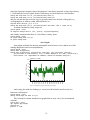
Scatter or Line Graphs
The scatter command, part of the twoway suite, is the workhorse of graph commands, and
really the workhorse of descriptive statistics (and regression diagnostics as well). Here’s a quick
example:
sysuse uslifeexp2, clear
scatter le year
where you can see immediately the impact of the Spanish Flu relative to various wars.
You can add options to pretty it up, if you like:
sysuse uslifeexp2, clear
scatter le year, subti("Life expectancy at birth, U.S.") note("1")
caption("Source: National Vital Statistics Report, Vol. 50 No. 6")
and there are a few hundred thousand ways you might modify that graph with options, so I won’t
go into detail. It’s all in the help files.
One of the common options on a scatter plot is to connect the dots:
sysuse uslifeexp2, clear
scatter le year, c(l)
and sometimes to suppress the dots after connecting them:
scatter le year, c(l) m(i)
40
45
life expectancy
50
55
60
65
Life expectancy at birth, U.S.
1900
1910
1920
Year
18
1930
1940
The last is so common, in fact, there is a separate command to make it easier to type:
sysuse uslifeexp2, clear
line le year
but note that the dots are graphed in the sort order of the data, which can result in some
unpleasant looking graphs unless you specify the sort option:
sysuse auto, clear
line mpg weight
line mpg weight, sort name(s)
The name option is handy when you want to have a number of graphs open at once for
comparison.
Density and Local Polynomial Graphs
The last graph (line mpg weight, sort) is getting close to specifying an empirical model:
mpg declines as weight increases. As useful as scatter/line plots and histograms are in small
datasets, they rapidly become untenable in large datasets. A good way to get sense of the
distribution of a variable (or a residual after a regression) or the functional relationships between
pairs of variables in a large dataset is to use kernel estimators like kdensity or lpoly. Kernel
estimators use subsets of the data and reweight to construct local estimates, for example of the
proportion of cars with mileage “near” 21 mpg (a kernel density estimator), or the effect of
another 100 pounds on mpg “near” 3000 lbs (a kernel regression estimator).
sysuse auto, clear
hist mpg, name(h)
kdensity mpg, name(k)
You can get the values that hist uses with the undocumented command
is handy for combining graphs:
0
.02
.04
.06
.08
.1
twoway__histogram_gen and then graph them with tw bar, which
twoway__histogram_gen mpg, bin(8) start(12) gen(f x)
tw bar f x || kdensity mpg
10
20
30
Density
40
kdensity mpg
The user-written kdens (ssc install kdens) offers even more flexibility than kdensity.
In Stata 10, local polynomial regression is performed with the command lpoly, but the nearequivalent command locpoly is available via findit (http://www.stata-journal.com/software/sj64) for prior versions.
net from http://www.stata-journal.com/software/sj6-4/
19
net inst st0053_3
line mpg wei, sort name(bumpy)
locpoly mpg wei, name(smooth)
Local polynomial smooth
10
Mileage (mpg)
20
30
40
Degree: 0
2,000
3,000
Weight (lbs.)
Mileage (mpg)
4,000
5,000
locpoly smooth: Mileage (mpg)
The lowess command is also available in Stata versions before Stata 10, but I’ve never liked
it as much, mainly because it does not offer the at() option with the generate() option, and does
not give the same control over kernels. The at() option and generate() option are especially
helpful if you want to overlay two smoothed graphs:
10
locpoly smooth: mpg
15
20
25
30
sysuse auto, clear
g m=(16+_n)*100 in 1/32
la var m "Weight"
locpoly mpg wei if for==1, nogr at(m) gen(mfor)
locpoly mpg wei if for==0, nogr at(m) gen(mdom)
line mfor mdom m, leg(lab(1 "Foreign") lab(2 "Domestic"))
1000
2000
3000
Weight
Foreign
4000
5000
Domestic
Bar Graphs
You can get simple bar graphs with graph
bar
but more flexibility with twoway
sysuse sp500, clear
gr bar high in 1/4, over(date)
20
bar:
where the legend on categories shows their numeric value (dates measured as days since January
1, 1960) instead of a more legible format. With twoway bar the defaults are a bit friendlier:
twoway bar high date in 1/4, yla(1300(20)1340) barw(.5)
twoway bar high date in 1/4, yla(1300(20)1340) barw(1.5)
and you can alter the data in clever ways to get total control over the look of the graph, e.g.
overlapping bars of arbitrary width, different labels, etc.:
replace date= date+(2-_n)/3 in 1/4
twoway bar high date in 1/4, yla(1300(20)1340) xla(14977 "Jan 2" 14979 Jan 5")
A related command is twoway
dropline:
sysuse sp500, clear
tw dropline change date in 1/57, yline(0, lstyle(foreground))
and a handy command when there is a lot of data is twoway
spike:
sysuse sp500, clear
tw spike change date in 1/57
tw spike change date
Area Graphs
Area graphs are handy for showing meaningful areas between a curve and an axis (if the
running integral has some real interpretation):
sysuse gnp96, clear
twoway area d.gnp96 date
twoway area d.gnp96 date, xla(36(8)164, angle(90)) yla(-100(50)200, angle(0))
yti("Billions of 1996 Dollars") xti("") subti("Change in U.S. GNP", position(11))
note("Source: U.S. Department of Commerce, Bureau of Economic Analysis")
Change in U.S. GNP
200
Billions of 1996 Dollars
150
100
50
0
-50
2001q1
1999q1
1997q1
1995q1
1993q1
1991q1
1989q1
1987q1
1985q1
1983q1
1981q1
1979q1
1977q1
1975q1
1973q1
1971q1
1969q1
-100
Source: U.S. Department of Commerce, Bureau of Economic Analysis
And a range plot with area shading (tw
functions is informative:
rarea)
is useful when the area between two
sysuse sp500, clear
twoway rarea high low date in 1/57
This is handy for custom standard error graphs (but see help
solution):
sysuse auto, clear
qui regress mpg weight
predict hat
predict s, stdf
21
lfitci
for an automated
0
10
20
30
40
gen low = hat - 1.96*s
gen hi = hat + 1.96*s
tw rarea low hi weight, sort color(gs14) || scatter mpg wei
2,000
3,000
Weight (lbs.)
low/hi
4,000
5,000
Mileage (mpg)
Note that we graphed the shaded area first and then the scatterplot. Typing
tw scatter mpg wei || rarea low hi weight, sort color(gs14)
would superimpose the shading on the scatter, obscuring the dots.
Mapping
There is a nice guide to mapping in Stata at
http://mysite.verizon.net/huebler/2005/20051106_tmap.html, and there are FAQs on the Stata
website (e.g. http://www.stata.com/support/faqs/graphics/tmap.html). The relevant commands
are tmap for Stata 8 and spmap for more recent Stata versions, both available from SSC.
cap ssc install tmap
cap copy http://pped.org/stata/uscoord.dta /uscoord.dta
use http://pped.org/stata/spop90.dta, clear
gen East=(LON>=-98)
tmap cho p if East==1, id(id) map(\uscoord.dta)
[0.56,2.46]
(2.46,4.58]
(4.58,6.55]
(6.55,17.99]
Adding Text and Lines
Many lines can be added with options xline() or yline(). See help added_line_options
and help added_text_options for more. Arrows can be added via tw pcarrow tricks.
22
The New Graph Editor
In Stata 10, you can click on a graph and add graphic elements such as text or lines
interactively, using the new Graph Editor, but there is no way to store those changes as
commands, so it behooves you to learn the command syntax approach. Otherwise, when you
change your graph, you’ll be stuck clicking and dragging and typing ad nauseam. I would
recommend you not use the new Graph Editor, unless there is no other way forward.
3. Looping, Programming, and Automating Output in Stata
Good Programming Style
Thm: Reproducibility, error reduction, ease of use, and portability all depend on good
programming style.
Cor 1: Don't type any parameter (a number or string of characters that you might later change)
more than 3 times in a program or do-file. If you do, you are inviting a situation where
you change 2 instances and forget the third, and never notice the output is flawed.
Cor 2: Comments are good, but clean code is better. Comments tell you what the programmer
intended, but might not help you fix or adapt the code easily. Clean code does both.
Cor 3: A little bit of programming sophistication goes a long way. If you are reformatting tables
of output more than once when the output changes, you would have been better off
programming the output (table layout and number display format) in the first place. If
you are doing the same thing over and over (similar regression, similar graphs, similar
paper topics), you are at risk of becoming a dull boy. Doing the same thing over and over
is what computers are for.
Looping
This is how you make the computer do your work for you, and save yourself some carpal
tunnel: Use foreach or forvalues, not for (note while and for still work, but are harder to
use, and the for command had some problems—just avoid it). foreach works beautifully, and is
simple:
foreach v in some list of stuff {
does this 4 times, for `v'="some" and `v'="list" etc.
presumably does something with `v' itself
}
Make sure the curly braces are as shown (no code after the first, and the second on a line by
itself).
Here's a fun example (though outdated, as tmap has been replaced by spmap):
qui ssc install tmap
cap copy http://pped.org/stata/uscoord.dta /uscoord.dta
use http://pped.org/stata/spop90.dta, clear
gen East=(LON>=-98)
gen West=(LON<-98 & id!=13 & id!=56)
foreach v in East West {
tmap cho p if `v'==1, id(id) map(\uscoord.dta)
graph rename `v', replace
*makes a popn map for the west, then the east
}
erase /uscoord.dta
The similar command forvalues steps through a numeric list:
23
forvalues v=1/10 {
does this 10 times, for `v'=1 and `v'=2 etc.
presumably does something with `v' itself
}
Note that forvalues v=1/10 { is equivalent to foreach v in 1 2 3 4 5 6 7 8 9
10 {
Perhaps handiest is the second syntax of foreach, i.e. one of the following:
foreach
foreach
foreach
foreach
foreach
lname
lname
lname
lname
lname
of
of
of
of
of
local lmacname {
global gmacname {
varlist varlist {
newlist newvarlist {
numlist numlist {
so you can store any list in a macro, or have Stata parse a variable list for you. Note also that
foreach v of numlist 1/10 {
is equivalent to
forvalues v=1/10 {
All of these loops can be nested: just make sure you use different names for the local macros
created:
foreach v of numlist 1/10 {
foreach v of numlist 1/10 {
di "Row `v' and Column `v' value is "
}
}
will obviously not work, but this is fine:
foreach r of numlist 1/10 {
foreach c of numlist 1/10 {
di "Row `r' and Column `c' value is "
}
}
See also the continue and break commands for exiting a loop prematurely or preventing
exit from a loop or program.
The levelsof command works very nicely with foreach to do something for every value
of a variable, e.g.
webuse nhanes, clear
levelsof race, local(r)
foreach v of local r {
svy, subpop(if race==`v’): tab sex higbp, row
}
Output: The file, estout, and xmlsave Commands
The file command allows you to read or write to text or binary files. This means that you
can write anything you can think of to a file. You could have a whole paper (text, tables,
graphics, etc.) written out by one do-file, in theory, or even write out a file that would be an
executable program (not that anyone would ever do that) and then run it.
In particular, you can write out in any format the output from tabulations or regressions
available via return or ereturn or built-in shortcuts like _b[var] (gives the coefficient on
var) or _se[var] (gives the SE on var). For example:
webuse nhanes2, clear
qui svy: tab race diab, row ci
mat rowpc=e(b)
file open d using /b.txt, write replace
24
file write d "Race" _tab "Percent Diabetic"
forv r=1/3 {
file write d _n "`: lab (race) `r''"
file write d _tab "`: di rowpc[1,`=`r'*2']'"
}
file close _all
type /b.txt
local excel="C:\Program Files\MSOffice2000\Office11\Excel.exe"
winexec `excel' \b.txt
And it would be easy to embed the preceding in a larger loop that stepped through a list of
diseases, and did tests of significance, etc., and then opened it all up in Excel, if you like that
kind of thing.
The estout command from SSC automates the creation of tables of coefficients from
estimation commands or of summary statistics, and is far better than crappy alternatives like
outreg. Install it with ssc install estout. This is a really useful command, and has myriad
options, so the command has its own website at http://fmwww.bc.edu/repec/bocode/e/estout/
with plentiful examples.
The xmlsave command allows you to save a Stata dataset in an XML file format: either
Stata's .dta or Microsoft Excel's SpreadsheetML format. So you can collapse your data into a
dataset of means by year, say, then save in Excel format.
A user-written command xml_tab (findit xml_tab) offers a way to write out various
formatted tables to Excel-type files. You may find it especially handy when used to create and
output a simple table of the means:
tabstat price mpg rep78 headroom trunk weight length, by(foreign) save
ssc inst tabstatmat, replace
tabstatmat A
matrix TAB=A'
xml_tab TAB, replace
where tabstat generates a table of means for the list of variables categorized by foreign.
tabstatmat saves the results to matrix A with three rows for Domestic, Foreign and Total. In
the columns of matrix A are the means for the listed variables. The transposed matrix A is the
matrix TAB, which xml_tab outputs into the default XML file. You can see more examples of
using xml_tab in xml_tab_example.do (findit xml_tab).
The program Command, and ado Files
Any bit of code you want to repeat should be coded as a program. So a bit of text, or a
number, should be coded as a macro, but some lines of code that, say, calculate convert some
amounts into real dollars, or write out a table of estimates, can be written as a program, and then
to run the code, you just type the name of the program:
cap program drop dtab
program dtab
syntax varname
webuse nhanes2, clear
qui svy: tab race `varlist', row ci
mat rowpc=e(b)
file open d using /b.txt, write replace
file write d "Race" _tab "Percent suffering from `varlist'"
forv r=1/3 {
file write d _n "`: lab (race) `r''"
file write d _tab "`: di rowpc[1,`=`r'*2']'"
}
file close _all
25
type /`varlist'.txt
end
Now you can type, e.g.
dtab diab
dtab heart
dtab highlead
ad infinitum. If you saved that bit of code in a file called dtab.ado, you could type those lines
(e.g. dtab diab) to get an instant table at the command prompt, or in an unrelated do-file. The
ado file loads a program automatically; that is how a lot of Stata's official commands are written
(and you can read their code, with the viewsource command, which is instructive, to say the
least). There's a lot more about program in the Programming manual, of course.
Automating Appendices
Michael Blasnick documented the MS Word trick of using a mail merge to put a series of
Stata output files into a Word document at http://www.stata.com/statalist/archive/200406/msg00301.html and http://ideas.repec.org/p/boc/asug05/14.html. I’ve used it in e.g. the
appendices of http://nber.org/papers/w13246, so I can attest that it can be quite handy in
circumstances where you have to produce a lot of pages of the same type of thing.
4. Estimators
We’ve followed the path of many stats courses, doing some tabs and some graphs as
exploratory data analysis, not worrying too much about standard errors or statistical significance.
However, a tab of y versus x or a graph of y versus x usually is designed to elicit information
about the “effect” of x on y. Thus, we don’t simply want to know what proportion of dropouts by
parent’s marital status, we want to know the effect of parent’s marital status on likelihood of
dropping out. Returning to our auto data, we don’t want to know the fuel efficiency by weight
class, we want to know what the effect of an extra 100 pounds is on fuel efficiency.
In fact, a tabulation is an estimator, in the same way that an OLS regression is, and you can
construct a confidence interval around a proportion (a tricky subject actually—see "Interval
Estimation for a Binomial Proportion" by Lawrence D. Brown, T. Tony Cai, and Anirban
DasGupta for details) from a tabulation, or test the equality of two proportions, using the tricks
shown in the answers to Day 1’s exercise 3.
There are various other programs to run hypothesis tests, including signrank, kwallis,
nptrend, ranksum, runtest, bitest, ttest, etc. For example to test equality of mean mpg
across foreign and domestic cars in the auto data, you can ttest mpg, by(for). If you want to
test the equality of means, however, the natural way to do that is in a regression, e.g. reg mpg
fore will test whether foreign cars get better gas mileage on average. See
http://www.ats.ucla.edu/stat/stata/webbooks/reg/default.htm for a gentle introduction to
regression models in Stata.
Regression and Testing Hypotheses
We’ve already run a regression by fitting a line on a graph.
sysuse auto, clear
tw lfitci mpg wei, by(for) || scatter mpg wei
is running a regression (actually two OLS regressions), and showing the results in a graphical
form. We could also
26
sysuse auto, clear
reg mpg wei if fore==1
est sto f1
reg mpg wei if fore==0
est sto f0
suest f0 f1
test [f0_mean]w=[f1_mean]w
or
gen forwei=fore*wei
reg mpg wei fore forw
test fore forw
both of which formally test that foreign and domestic cars exhibit the same relationship between
mpg and weight, but the first approach allows the estimated error variance (the variance of
residuals y-Xb) to vary across the two subsamples. See also
http://www.stata.com/statalist/archive/2007-07/msg00125.html
http://www.stata.com/statalist/archive/2006-12/msg00147.html
http://www.stata.com/statalist/archive/2006-12/msg00170.html
for more discussion.
The mfx command computes marginal effects, which for linear regression is just the
coefficient, so doesn’t have much effect until you run a nonlinear model. Note that to test the
marginal impact when you have interaction terms or powers (e.g. squares or cubes), you need to
do a little calculus before you specify a test command. The test command conducts a Wald
test of joint significance, or any combination of linear hypotheses (see help test for more) e.g.
test wei=forw
test for, accum
tests that the effect of weight is exactly twice as big among foreign cars. Nonlinear tests can be
done using nlcom.
To learn various techniques used to assess your model fit, you might want to read help
regress postestimation. and see the manual at [R] regress postestimation (particularly
helpful are scatterplots of residuals such as rvfplot and rvpplot).
To compare the importance of various coefficients, you might want to use the beta option
of regress, which asks that standardized beta coefficients be reported instead of confidence
intervals. The beta coefficients are the regression coefficients obtained by first standardizing all
variables to have a mean of 0 and a standard deviation of 1. Or you might want to get the SPost
commands from http://www.indiana.edu/~jslsoc/stata that allow you to do more. Type findit
spost9_ado in Stata to get a short list.
We could also graph various pieces of the regression output directly, if we wanted to:
tw function y=_b[_cons]+_b[wei]*x*2000, range(1000 5000) || scatter mpg wei if fore==0
or save the coefficients and standard errors in macros for later calculations. You can use all the
estimation results, though you may have to do some calculations yourself on the raw numbers
(see help ereturn).
For now, let’s focus on the first regression: the relationship between weight and (supposed)
fuel efficiency for foreign cars:
reg mpg wei if fore==1
tw lfit mpg wei if fore==1 || scatter mpg wei if fore==1
27
and note that the spread of errors is much larger for lower-weight cars, i.e. we see
heteroskedasticity, which results in incorrectly calculated standard errors—but it is a common
enough condition to have an easy solution: use the robust option (do not look for robust
regression—this is something else altogether).
reg mpg wei if fore==1, robust
Note that the standard errors are smaller when using robust here, which is unusual. Usually,
a model specified without using robust will have improperly small standard errors, and lead
researchers to find effects (reject the null of b=0) where there is no evidence of effects. Note the
use of “no evidence of effects” instead of “no effects,” which we cannot conclude when we fail
to reject the null.
In general, computing heteroskedasticity-robust standard errors does not absolve
misspecification (as I have committed above, since I know mpg is not a good measure of fuel
efficiency, since the inverse gallons per mile would be a better measure of energy consumption).
But it does seem to cover a multitude of misspecification-type sins in simulations, and its smallsample properties are surprisingly good.
The heteroskedasticity-robust standard errors calculated here are also called Huber-White
standard errors, and the estimator the Huber-White or “sandwich” estimator, after
Huber, P. J. 1967. The behavior of maximum likelihood estimates under nonstandard conditions. In
Proceedings of the Fifth Berkeley Symposium on Mathematical Statistics and Probability.
Berkeley, CA: University of California Press, vol. 1, 221–223.
White, H. 1980. A heteroskedasticity-consistent covariance matrix estimator and a direct test for
heteroskedasticity. Econometrica 48: 817–830.
or sometimes White standard errors, by folks who don’t know Huber published first.
It’s a good general rule to always use the robust option—if there is no heteroskedasticity,
you will get the same answer with or without the robust option.
One thing heteroskedasticity-robust standard errors don’t correct for is clustering of errors—
when the error on an individual observation is correlated with errors on other individual
observations. If multiple individuals are observed within households, there is almost always
clustering of errors at the household level. Think of an x variable like a tax incentive to work
more, and its effect on labor supply within a household—if it has an effect of increasing hours by
20% for a person living alone, it is almost certain not to increasing hours worked by each
individual in a large household by 20% (some of them won’t even be working), and may even
depress the labor supply response of another household member—the bigger response by one
person will be negatively correlated with a smaller (or opposite-signed) response by another.
Clustering also arises from survey design, and you can account for that type of clustering
using the svy commands, which also specify weights and stratification. A useful way to correct
for clustered error without using svy is to use the cluster( ) option to get cluster-robust
standard errors (this estimator is a direct result of Huber 1967 but sometimes called Rogers
standard errors because Rogers 1993 was the first to put the details in writing):
The cluster( ) option requires you to specify (by putting a variable name between the
parentheses) the level at which the clustering of errors occurs—a good rule of thumb is that you
need at least 50 clusters to get reliable estimates, but you want to cluster at the highest level
where clustering is likely. In a regression of individual data on state-level regressors, you
probably want to cluster at the state level.
28
The cluster-robust estimator of standard errors is also a “sandwich” estimator, but the
ingredients are a bit different. Essentially, you assume that errors are independent across clusters,
and use errors within each cluster to estimate the within-cluster correlations.
Panel regression
Longitudinal data or panel data, has single units observed at multiple points (in time,
usually) and allows you to control for all kinds of unobservable factors that don’t vary over time.
The suite of XT commands (see help xt and the XT manual) offer a whole panoply of
techniques, but we’ll see two today.
use http://fmwww.bc.edu/ec-p/data/macro/abdata.dta
loads some macro data on employment in Britain.
tsset id year
tells Stata that id identifies units, indexed i in textbooks, and year identifies the points at
which we observe them, indexed t in textbooks. Now regress industry output on capital stock and
employment:
xtreg ys k n, fe
xtreg ys k n, fe robust
and note that you have controlled using fixed effects for any firm characteristics that do not
change over time (a whole host of potential x variables spring to mind). If you wanted to
measure the effect of some fixed firm characteristic, you would have to use another estimator—
perhaps a random effects estimator like xtreg ys k n, re robust.
See http://www.ats.ucla.edu/stat/Stata/faq/revsfe.htm for a simple take on the fixed-effects,
between-effects, and random-effects estimators. For more, read a textbook by Wooldridge. Also
note that if you ever run a random-effects model, you MUST run a Hausman test (see help
hausman) to show that it is appropriate.
If you want to run a fixed-effects regression using pweights, use an equivalent command
called areg (see help areg for the syntax). As of Stata 10, xtreg also allows pweights, but
requires that they be constant within panel (areg does not).
areg ys k n, absorb(id) robust
More on clustering
In panel regressions, you should always cluster on the ID variable, or a higher (more
inclusive) level if you can (i.e. you’ve got at least 50 units), since the cluster-robust variance
estimator corrects for arbitrary serial correlation.
areg ys k n, absorb(id) robust
areg ys k n, absorb(id) cluster(id)
Some might hint that you should “always cluster your standard error on the same level on
which you would use fixed effects” or somesuch, which is not the case. For example, if you
observed individuals (who didn't move) over time, and you regressed their outcomes on countylevel variables, you might want to include fixed effects for individual people, but cluster on the
county level (accounting for the intra-county clustering of errors over time and people).
A useful treatment for the general case is “Robust Standard Error Estimation in FixedEffects Panel Models,” by Gábor Kézdi, originally published as a working paper in about 2001,
and usually cited that way, but now with a publication date of 2004, and a ridiculously long
URL, which shows that the cluster-robust estimator performs well even in the absence of
clustering (i.e. there is no real danger when specifying the cluster option).
29
Another frequently cited source is Arellano (1987). "Computing robust standard errors for
within-groups estimators." Oxford Bulletin of Economics and Statistics, 49(4): 431–434.
Quoting Mark Shaffer, “it's also worth adding that Stock and Watson, in an important little
paper that appeared earlier this year, showed that the standard heteroskedasticity-robust
estimator, available in Stata with the -robust- option, is inconsistent for the fixed effects
estimator. Interestingly, the problem does not extend to the cluster-robust estimator, which is
also heteroskedasticity-robust. Thus, if you are doing fixed effects and want your SEs to be
robust to heteroskedasticity, you should avoid robust and use cluster() instead, and get SEs
that are robust to both heteroskedasticity as well was intra-group correlation.” The reference
there is James H. Stock, Mark W. Watson (2006), "Heteroskedasticity-Robust Standard Errors
for Fixed Effects Panel Data Regression", NBER Technical Working Paper No. 323.
http://www.nber.org/papers/T0323
If you think clustering happens along more than one dimension, for example there is
autocorrelation within panel (my error today is related to my error yesterday) and across panels
at a point in time (my error today is related to my wife’s error today), you can try out a two-way
clustering approach by Cameron, Gelbach, and Miller:
http://www.nber.org/papers/t0327
http://glue.umd.edu/~gelbach/ado/cgmreg.ado
but this is an active research area, so you are unlikely to get much help if you run into trouble.
You can get nested clustering (households within counties within states, for example) using
svy but my impression is that nested clustering makes little difference if you are able to cluster at
the highest level (state in the example) and clusters are of roughly equal sizes.
Logit, Probit
You might also regress dropout on parent’s marital status, but that is a bad idea whenever
you have binary outcomes (two outcomes, usually 0 and 1 meaning false and true) since the
linear probability model (LPM):
reg dropout pmarr, r
produces predicted probabilities that lie outside the [0,1] interval, among other reasons.
Instead, use a logit or probit. Which? Well, it makes little difference, usually, but a logit
is usually faster and easier to interpret. You can get odds ratios by specifying the or option on
logit, or using the logistic command.
logit dropout pmarr, r
logit dropout pmarr, r or
logistic dropout pmarr, r
You can get marginal effects for probit using the dprobit command, though you will
probably want to use the mfx command to compute marginal effects for either logit or probit.
The marginal effects will likely be wrong if you have any indicators (dummy variables) or
interactions (see http://www.unc.edu/~enorton/NortonWangAi.pdf and its references for more
details). Here’s an old email on computing the marginal effect for a single indicator variable in a
probit model:
To compute the marginal effect (change in probability) for a probit or logit, most will just calculate f(xbar beta)
and multiply by the reported coef, but that is not right.
For a probit with
y* = b*X + g*D + e
30
y = 1 iff y*>0
where X is a matrix of regressors, and D is a dummy variable representing treatment, the marginal effect of D
is measured in a sample as
Ei [y|D=1, X=Ei [X]]- Ei [y|D=0, X=Ei [X]]
where the Ei[.] operator denotes the sample mean. This is equivalent to
Ei [Φ (b*Xi +g) - Φ(b*Xi )]
where Φ (.) is the cumulative normal. For g small, this can be approximated as
Ei [φ (b*Xi) ] g
but the quality of this approximation will vary with the size of g and the curvature of the function Φ (.) in the
vicinity of b*Xi or (b*Xi +g). This quantity is sometimes approximated as
φ (Ei [b*Xi ]) g
the expression in my prior email (which I called f(xbar beta) multiplied by the reported coef), but this is a very
rough approximation indeed. If b*Xi is uniformly distributed on [-1,1] the expectation of φ (b*Xi) is 0.68 and the
normal density evaluated at Ei [b*Xi ] is 0.4 (for other cases, e.g. a wider interval, the approximation might be
substantially worse).
But g need not be small. If the coefficient on the dummy variable is 5 or 10, the first step of the approximation
might be quite a poor one. If b*Xi is tightly distributed around zero, and g is large, the true marginal effect will be
close to one half. The first version of the approximation would give the marginal effect as 0.4 times g, so if g were
10 the marginal effect would be 4. In general, the first approximation might yield estimated marginal effects much
greater than one, which are obviously poor estimates.
In short, predict probabilities and graph them, don’t try to compute simplistic marginal
effects at the mean.
If your dependent variable has multiple values, you might want mlogit (if the categories are
not naturally ordered) or ologit (if they are), but see also gologit2 (findit gologit2). If
your model has binary outcomes measured multiple times for each unit, you may have panel data
(see help xtlogit) or choice data (see http://stata.com/help.cgi?asclogit).
Poisson/GLM
Using poisson sounds odd to lots of folks, but the idea is this: if you have a nonnegative
dependent variable that’s mostly small, but has a few big values, you might be tempted to take
the log and regress the log of y on X. But if there are any zeros, they are now missing. If you
assume E[y|X]=exp(Xb) as you just did when taking the log, then you should run poisson
regression, which does not drop zeros. The coefficients are interpreted just as if you had taken
the log of y: a one-percent change in x is associated with a b/100 percent change in y.
You would not want to use tobit in this situation (though you will see it done a lot) since
the assumptions are not satisfied: tobit is for the case when we don’t observe the true value of y
because it is censored, not because it is truly zero and we foolishly took the log of it.
The original idea of poisson is to model response variables that are counts (number of kids,
number of cigarettes, number of doctor visits, how many dollars, etc.) but the model works well
as long as E[y|X]=exp(Xb) which is true in a much broader class of problems. See Wooldridge
2002 (http://www.stata.com/bookstore/cspd.html) p.651 and surrounding text: “A nice property
of the Poisson QMLE is that it retains some efficiency for certain departures from the Poisson
assumption,” etc.
You can get the same answers as poisson (or logit or other related commands) using
Generalized Linear Models via the command glm, which estimates
31
E(y)=F(Xb)
for a variety of different functions F() and error distributions. The key point is that there is a
linear combination of x variables that F() is applied to.
When you have a bunch of zeros or variance substantially greater than the conditional mean,
you may want models in which poisson may be nested, such as nbreg zip or ztp.
IV Regression
The thing that is wrong with most of the regressions you will run is that the RHS variables
are endogenous. That is, they are correlated with the error term. Either you left an important
variable out, or y and x are simultaneously determined (as part of a system of supply and
demand, for example), or x is measured with error (that never happens, right?), or any of a large
number of other plausible conditions are met where your coefficient on x is biased. What now?
Well, you get $10 million to run a massive experiment, right? You want to do an experiment
because an experiment gives an unbiased estimate, but experiments are not only costly, they can
also be downright infeasible, so we turn to quasi-experimental methods (see
http://www.urban.org/toolkit/data-methods/quasi-experimental.cfm).
The most frequently used is instrumental variables (IV) regression, where you find
something that moves x around, but has no direct effect on y. This is your excluded instrument.
If you can find a few, you can conduct an overid test to see if they are any good at all (see
http://fmwww.bc.edu/ec-p/WP545.pdf for more details, and other tests you should run). Good
instruments are hard to come by, and even once you’ve got one, it may be weak (see
http://www.stata.com/meeting/5nasug/wiv.pdf for more). Note that the official Stata 9 command
ivreg does not offer the full range of diagnostics for IV regression—type findit ivreg2 to get
the good one, based on ivreg but augmented (Stata 10 has ivregress which offers weak
instrument diagnostics but still does not offer the full range of stuff that ivreg2 can). Even if
you can conclude you don’t have weak instruments, your estimates are still biased (though
consistent now), just a bit less than they were before, and the price you’ve paid is a large increase
in variability.
0
.02
.04
.06
.08
Estimated effect where true effect is 12
-10
0
10
20
30
40
50
Sampling Distrib of Coef
IV beta
OLS beta
The upside is, as you add more data, you will get closer to the true answer, which won’t
happen in the standard regression, and your inference will be approximately correct, if lowpowered, whereas tests after the standard regression may be way off.
32
There are also panel versions of the IV estimator—type findit xtivreg2 to get the good
one for fixed effects.
use http://fmwww.bc.edu/ec-p/data/macro/abdata.dta
xtivreg2 ys k (n=l2.n l3.n), fe small first cluster(id)
Dummy endogenous variables (endogenous indicator variables) are not a problem for the
consistency of IV though you can get improved efficiency using Procedure 18.1 of Wooldridge
2002 (http://www.stata.com/bookstore/cspd.html), pp.621-625. If you have a single endogenous
indicator variable and a binary outcome, you may want treatreg instead. If your outcome
variable is bounded or discrete, you may want the GLM equivalent of IV which is estimated by
qvf as described in Stata Journal Volume 3, Number 4 and at http://www.stata.com/merror/. Try
not to use ivtobit.
Matching and RDD
For more quasi-experimental methods, see findit psmatch2 (see also
http://www.stata.com/statalist/archive/2007-06/msg01026.html) and findit nnmatch (see also
http://www.stata.com/statalist/archive/2007-04/msg00011.html and
http://www.stata.com/meeting/5nasug/Imbens_stata_06july.pdf ) for matching methods, and see
http://www.urban.org/toolkit/data-methods/regression.cfm and http://nber.org/papers/t0334 and
http://www.nber.org/papers/t0337 for more on regression discontinuity methods.
Mixed models
Mixed models have a mixture of fixed and random effects, and are often called multi-level
models or hierarchical models (the software HLM is designed to just do these; UI has two copies
of this software, but they are not on the network). The command xtmixed is for multi-level
linear models, and has a more flexible but slower user-written analog gllamm (findit gllamm
and http://www.gllamm.org/) that will also do nonlinear models. There are a few books on using
these methods in Stata, including http://www.stata-press.com/books/mlmus.html, and a full
discussion would be another multi-day class. Stata 10 now offers some nonlinear mixed
models—see http://www.stata.com/help.cgi?xtmelogit,
http://www.stata.com/help.cgi?xtmepoisson
5. Manual Bootstrap Estimates and Monte-Carlo Simulation
33
6. Mata Programming
Introduced with Stata 9, Mata is a separate programming language within Stata that is
compiled, and runs with speed comparable to C and other high-level languages. Its syntax is
similar to C, and it offers a library of convenient matrix functions. As of 25 June 2007, Stata 10
offers a general optimize command in Mata, which is useful in a variety of ways. The entire
three-volume set of Mata manuals is online; just type help mata to get started. However, the help
files do not have many helpful examples. Below are two simple examples, demonstrating a
small fraction of Mata’s tremendous capacities: (1) writing out a GMM estimator, and (2)
solving a complicated function.
Mata is fast, because functions are compiled, rather than interpreted. I.e. if you look at what
Stata sees in the pre-Mata "ado language" version of a program, you see code like the text on the
left; if you look at what Stata sees in a Mata function, you see bytecode like on the right (zeros
and ones, really, but easier to read in this formatted hexadecimal way).
forvalues j = 1/`p' {
tempvar x`j'
2220 7b0d 0a09 0971 7569 2072 6570 6c61
qui gen double `x`j'' = .
6365 2060 6b61 7267 2720 3d20 302e 3520
local xs `xs' `x`j''
6966 2061 6273 2872 6f75 6e64 2860 6172
}
6727 2c31 652d 3829 293c 3120 2620 6074
qui gen double `arg' = .
qui gen double `karg' = .
forvalues i = 1/`n' {
6f75 7365 270d 0a09 7d0d 0a09 656c 7365
qui replace `arg'=(`x'-`xgrid'[`i'])/`h' if `touse'
207b 2009 0909 092f 2f20 6570 616e 6563
qui replace `karg' = .
686e 696b 6f76 0d0a 0909 6c6f 6361 6c20
if "`kern'" == "biweight" {
636f 6e31 203d 2033 2f28 342a 7371 7274
local con1 = .9375
qui replace `karg' = `con1'*(1-(`arg')^2)^2 /*
*/ if `touse' & abs(round(`arg',1e-8))<1
}
Of course there is a readable version of the Mata code, before it is compiled into “bytecode”
that is optimized for the computer to read. You write Mata in the readable version, and then
Stata compiles into the bytecode before running it. The first time you run your newly written
programs, there may be no speed advantage, but every subsequent time, it will run about 2 to 10
times faster.
The syntax of Mata is quite different from Stata's "ado language" but still fairly easy,
especially if you have used C or C++ before.
34
Interactive Use
You can enter Mata in several ways; essentially type mata and then type Mata commands
until you’re done in Mata, then type end.
For example, to multiply two matrices, you could type in Stata:
matrix a=(1,2,3)
matrix aa=a’*a
matrix list aa
or you could type:
mata
a=(1,2,3)
a'a
end
to get the same output from Mata. Note that to get the output of some calculation, you can just
type the calculation. To assign it to some named object, just type name=result. We could have
also typed:
mata
a=(1,2,3)
aa=a'a
aa
end
where we first assign the result to a named entity, then get Mata to display the named entity by
simply typing its name (the simplest form of calculation, if you will, is just the identity function).
Or we could type:
mata
a=(1,2,3)
aa=a'a
st_matrix("A", aa)
end
matrix list A
where we create a matrix A in Stata (from the Mata matrix aa), exit Mata, and then display
the resulting calculation in Stata. This suggests the basic procedure for most interactions—do all
the calculations you can in Mata, to improve speed, then return them in Stata.
Mata has all the matrix functions of Stata, plus a lot more. Importantly, there is no limit on
the size of matrices, and matrices can contain strings or real/complex numbers.
35
Defining New Mata Functions and Type Declarations
You make a new function in Mata like so:
type name(arguments)
{
contents
}
where type is the type of entity the function returns, such as a matrix, or the special type void,
meaning the function returns nothing. The type of a Mata variable has two pieces: the element
type and organizational type (choose any one from each column):
eltype
-----------transmorphic
numeric
real
complex
string
pointer
------------
orgtype
---------matrix
vector
rowvector
colvector
scalar
----------
The default is the most general type: a transmorphic matrix, where transmorphic means that
the matrix can be real, complex, string, or pointer; and matrix means that the organization is to
be r X c, r ≥ 0 and c ≥ 0. Here's an example function that swaps rows in a matrix:
real matrix swaprows(real matrix A, real scalar i1, real scalar i2)
{
B = A
v = B[i1, .]
B[i1, .] = B[i2, .]
B[i2, .] = v
return(B)
}
but all those type declarations are optional, so you could also write:
swaprows(A, i1, i2)
{
B = A
v = B[i1, .]
B[i1, .] = B[i2, .]
B[i2, .] = v
return(B)
}
All of those variables created within a Mata function can also be declared to have a
particular type. See help m2_declarations for more info.
36
Every variable created within a Mata function is "private" meaning its scope is just within
the function, like a local macro. You can also declare variables to be global by using the
external declaration, which is a useful but dangerous way of passing info back and forth
between programs. Useful because you don't have to pass arguments, dangerous because if you
accidentally modify a global variable, it's gone. For example, in a complex program, if you
create two globals with the same name, you will be replacing the first with the wrong values (the
values of the second), and may get some errors that are hard to track down to their source.
Void Functions
One common type of function is the void function, which returns nothing. For example,
void iv_pois(todo,b,crit,g,H)
{
external y,X,Z,W
m=((1/rows(Z)):*Z'((y:*exp(-X*b') :- 1)))'
crit=(m*W*m')
}
declares that the function iv_pois has five arguments (two of which are used inside the function,
but all must be well-defined for the function to operate without spitting out an error message).
Then it says there are four globals it's going to use, does some calculations to modify some
variable crit, and that's it.
That particular function calculates the value of a Generalized Method of Moments objective
function, also called a criterion function.
GMM Estimation Using Mata
The Generalized Method of Moments (GMM), briefly, supposes that there are some
population moments that we can try to match in our sample by a good choice of some parameter
vector, e.g. in OLS where the population model is
E(y) = Xβ
or with a mean-zero error term
y = Xβ + ε
the usual assumption is that E(X'ε) = 0 in the population. So we can try to make the sample
analog true via a good choice of b in an equation
y = Xb + e
i.e. we try to make the mean of the vector m = X'e as close to zero as possible. The justification
for this approach is given by Hansen (1982) 1 .
1 Hansen, Lars Peter. 1982. "Large sample properties of generalized method of moments
estimators." Econometrica 50(3): 1029-1054. See also for more accessible discussions Hansen,
Bruce E. 2000. "Econometrics. 1st ed." Madison, WI: [http://www.ssc.wisc.edu/
bhansen/notes/notes.htm] and Baum, C.F., M.E. Schaffer, and S. Stillman. 2002. "Instrumental
variables and GMM: Estimation and testing." [http://fmwww.bc.edu/ec-p/wp545.pdf] and 2007.
"Enhanced routines for instrumental variables/GMM estimation and testing."
[http://fmwww.bc.edu/ec-p/wp667.pdf], both published in the Stata Journal.
37
It's not always possible to make a vector equal to zero, so instead we try to make the sum of
squared deviations from zero as small as possible, i.e. instead of choosing b to set m=0 we
choose b to minimize (m'Wm) where W is some weight matrix. Each W defines a different
GMM estimator. Choosing a weight matrix to be the inverse variance estimate leads to the most
efficient GMM estimator.
The instrumental variables (IV) version is a population model
y = Xβ + ε
plus the assumption that E(Z'ε) = 0 in the population. We can try to make the sample analog true
via a good choice of b in an equation
y = Xb + e
i.e. we try to make the mean of m = Z'e = Z'(y-Xb) as close to zero as possible by minimizing the
real-valued function m'Wm with our choice of b.
As another example, consider the population model
E(y) = exp(Xβ)
which is the assumption in Poisson regression (like regressing the log of y on X, but y=0 is not a
problem). Usually we specify an error term with mean 1 like so:
y = exp(Xβ)ε
Note that if ν=exp(ε) then y = exp(Xβ)exp(ν) =exp(Xβ + ν) so ln(y) = Xβ + ν if y>0, which is
why I say Poisson regression is like regressing the log of y on X.
The assumption for an IV version of Poisson regression is that E(Z'υ) = 0 in the population,
where υ is the mean-zero error y/exp(Xβ)-1. So we can try to make the sample analog true via a
good choice of b in the equation
y = exp(Xb)e
i.e. we try to make the mean of m = Z'u = Z'(y/exp(Xb)-1) as close to zero as possible. Using a
weight matrix W = (Z'Z)-1, we minimize the real-valued function m'Wm by choosing b.
It turns out to be pretty easy in Mata to minimize or maximize some arbitrary function.
Having already defined a function iv_pois that takes a parameter b and calculates the real valued
function crit=(m'Wm) given b, we just need to tell Mata that we want to minimize crit with our
choice of b.
We need Z and X and y matrices: these are matrices of data, which we can form from the
variables on a Stata dataset like so:
clear all
use http://fmwww.bc.edu/ec-p/data/wooldridge/card
g tousename=!mi(wage,educ,nearc4)
mata
y = st_data(., "wage", "tousename")
X1 = st_data(., "educ", "tousename")
Z1 = st_data(., "nearc4", "tousename")
Then we can add a constant term to both the X and Z matrices like so:
cons=J(rows(X1),1,1)
X = X1, cons
38
Z = Z1, cons
and calculate the weight matrix W:
W=rows(Z)*cholinv(Z'Z)
Then pick some arbitrary starting vector, say a vector of zeros:
init=J(1,cols(X),0)
where the only real limitation on a starting vector in numerical optimization is that the objective
function has to be defined in a neighborhood of that starting value, and that is always true in this
problem for a zero vector, since exp(Xb)=1 for b=0 and exp(Xb) is smooth in b at b=0.
Then we declare a new variable to hold our optimization problem, and call a few functions
to set up the type of optimization we want. Then the function optimize() finds the optimum and
returns the vector b that optimizes the function. Let's just assign that to a new variable p. We
can report the result by just typing p in Mata.
S=optimize_init()
optimize_init_evaluator(S, &iv_pois())
optimize_init_which(S,"min")
optimize_init_evaluatortype(S,"d0")
optimize_init_params(S,init)
p=optimize(S)
The evaluator is designated as iv_pois in the second line, and we specify minimization in the
third line. The fourth line is more interesting. "d" type evaluators max/minimize a real-valued
function, and "v" type evaluators a vector-valued function.
evaluatortype
Description
-----------------------------------------------------------"d0"
function() returns scalar value
"d1"
same as "d0" and returns gradient rowvector
"d2"
same as "d1" and returns Hessian matrix
"v0"
function() returns colvector value
"v1"
same as "v0" and returns score matrix
"v2"
same as "v1" and returns Hessian matrix
In some statistical applications, "v" type evaluators are more convenient to code than "d"
type, particularly since one tends to think of a dataset of values arranged in matrix X, the rows of
which are observations. A function h(p, X[i,.]) of a parameter p can be calculated for each row i
separately, as with a log likelihood, and it is the sum of those resulting values that forms the
function f(p) that is to be maximized or minimized. All of Stata's maximum likelihood routines
are being rewritten in this way.
39
The previous optimization problem can all be wrapped in a function that can be called from
within Stata like so:
void i_pois(string scalar depvar, string scalar x, string scalar z, string
scalar tousename, string scalar beta)
{
external y,X,Z,W
y = st_data(., tokens(depvar), tousename)
X1 = st_data(., tokens(x), tousename)
Z1 = st_data(., tokens(z), tousename)
cons=J(rows(X1),1,1)
X = X1, cons
Z = Z1, cons
W=rows(Z)*cholinv(Z'Z)
init=J(1,cols(X),0)
b=init
S=optimize_init()
optimize_init_evaluator(S, &iv_pois())
optimize_init_which(S,"min")
optimize_init_evaluatortype(S,"d0")
optimize_init_params(S,init)
p=optimize(S)
st_replacematrix(beta,p)
}
where now we pass to the function i_pois the list of variables that form X, Z, and y, and an
indicator for which observations we want to include (tousename), then once the optimization is
done, we store the parameter vector in the Stata matrix designated "beta" (the name of which we
also passed as an argument to the function i_pois).
The above is most of the SSC program ivpois (ssc install ivpois). The remainder is a
matter of parsing options, error-checking, and returning results.
So a new GMM estimator that you read about in the econometrics literature is a matter of a
few hours to program, once you get the hang of the most common elements of the language (i.e.
the first program might take a matter of a day or two to write, but the second an hour or two).
40
Solving Functions
The foregoing GMM discussion also suggests a way to solve some complicated function,
e.g.
f(p) = g(q)
where f and g are real-valued functions of row vectors p and q, writing
h(r) = f(p) – g(q) = 0
where r = (p,q), and then we can find solutions (or near-solutions for insoluble problems) by
minimizing
h(r)2
with our choice of r.
Here's a silly example to calculate the solution to ln(r)=0
void obj(todo,b,crit,g,H)
{
crit=ln(b)^2
}
init=5
S=optimize_init()
optimize_init_evaluator(S, &obj())
optimize_init_which(S,"min")
optimize_init_evaluatortype(S,"d0")
optimize_init_params(S,init)
optimize(S)
Note in the above that if you started at 0 you would get an error in this case, since ln(0) is
undefined. Everything would look fine until the last command, when you would see:
: optimize(S)
initial values not feasible
r(1400);
In general, of course, there is no guarantee that an optimum is unique, so if it is possible that
there are multiple solutions to h(r) = 0 you would have to start the optimization at many
appropriately chosen starting points to see if the optimizer finds different optimal parameter
vectors.
41
Suppose you wanted to find the zeros in
y = x2 – 5x + 4
and you were too lazy to use the quadratic formula (I chose this problem, of course, because its
analytic solution is so easy, whereas the numerical methods are trickier). You could just type
void q(todo,b,crit,g,H)
{
crit=(b^2-5*b+4)^2
}
sol=J(1,0,0)
void grid(n1,n2)
{
external sol, p
for (i=n1; i<=n2; i++) {
init=i
S=optimize_init()
optimize_init_evaluator(S, &q())
optimize_init_which(S,"min")
optimize_init_evaluatortype(S,"d0")
optimize_init_params(S,init)
p=round(optimize(S),10e-4)
if (!anyof(sol, p)) {
sol=(sol,p)
}
}
sol
}
grid(-10,10)
The above code does the optimization for every starting value on a grid over the integers -10 to
10 (and saves any solutions that are new to a Mata variable sol, then reports its values). A
function that took a vector as an argument would be no harder to specify (though the appropriate
grid search might be harder to specify).
42