Download Learning Stata

Learning Stata
Timberlake Consultants
E. HENGEL & M. WEEKS
Faculty of Economics
University of Cambridge
Harley Mason Room
Corpus Christi College
25 March 2014
Contents
1
Stata
1.1
Interface . . . . . . . . . . . . . . . . . . . . . . . . . . . .
1.2
Help . . . . . . . . . . . . . . . . . . . . . . . . . . . . . .
1.3
Syntax . . . . . . . . . . . . . . . . . . . . . . . . . . . . .
2
Data
2.1
2.2
2.3
2.4
2.5
2.6
2.7
2.8
2.9
2.10
1
1
3
7
.
.
.
.
.
.
.
.
.
.
11
11
12
12
13
13
15
16
19
20
26
3
Analysis
3.1
Mean . . . . . . . . . . . . . . . . . . . . . . . . . . . . . .
3.2
Correlation . . . . . . . . . . . . . . . . . . . . . . . . . .
3.3
Regression . . . . . . . . . . . . . . . . . . . . . . . . . . .
29
29
31
32
4
Stored results
4.1
r-class commands . . . . . . . . . . . . . . . . . . . . . . .
4.2
e-class commands . . . . . . . . . . . . . . . . . . . . . .
4.3
The four flavours of saved results . . . . . . . . . . . . . .
37
37
38
39
5
Tables
5.1
Basic tables . . . . . . . . . . . . . . . . . . . . . . . . . .
5.2
Advanced tables . . . . . . . . . . . . . . . . . . . . . . .
43
43
45
6
Graphs
6.1
Histograms . . . . . . . . . . . . . . . . . . . . . . . . . .
6.2
Box plots . . . . . . . . . . . . . . . . . . . . . . . . . . .
6.3
Scatter plots . . . . . . . . . . . . . . . . . . . . . . . . . .
53
53
55
56
7
Automating tasks
61
Loading example data
Browsing data . . . . .
Saving data . . . . . .
Loading real data . . .
Importing data . . . .
Renaming data . . . .
Labelling data . . . . .
Ordering data . . . . .
Creating data . . . . .
Missing data . . . . . .
.
.
.
.
.
.
.
.
.
.
.
.
.
.
.
.
.
.
.
.
i
.
.
.
.
.
.
.
.
.
.
.
.
.
.
.
.
.
.
.
.
.
.
.
.
.
.
.
.
.
.
.
.
.
.
.
.
.
.
.
.
.
.
.
.
.
.
.
.
.
.
.
.
.
.
.
.
.
.
.
.
.
.
.
.
.
.
.
.
.
.
.
.
.
.
.
.
.
.
.
.
.
.
.
.
.
.
.
.
.
.
.
.
.
.
.
.
.
.
.
.
.
.
.
.
.
.
.
.
.
.
.
.
.
.
.
.
.
.
.
.
.
.
.
.
.
.
.
.
.
.
.
.
.
.
.
.
.
.
.
.
.
.
.
.
.
.
.
.
.
.
.
.
.
.
.
.
.
.
.
.
.
.
.
.
.
.
.
.
.
.
7.1
7.2
8
9
Do-files . . . . . . . . . . . . . . . . . . . . . . . . . . . .
profile.do . . . . . . . . . . . . . . . . . . . . . . . . . . .
Programming
8.1
Macros . . . . . . . . . . . . . . .
8.2
Compound double quotes . . . .
8.3
Looping, branching and indexing
8.4
Programs . . . . . . . . . . . . .
61
63
.
.
.
.
67
67
71
72
78
Appendix
9.1
Operators . . . . . . . . . . . . . . . . . . . . . . . . . . .
9.2
Expressions . . . . . . . . . . . . . . . . . . . . . . . . . .
9.3
Commands . . . . . . . . . . . . . . . . . . . . . . . . . .
81
81
81
82
.
.
.
.
.
.
.
.
.
.
.
.
.
.
.
.
.
.
.
.
.
.
.
.
.
.
.
.
.
.
.
.
.
.
.
.
.
.
.
.
.
.
.
.
.
.
.
.
.
.
.
.
Bibliography
85
List of Figures
1.1
1.2
Stata’s interface . . . . . . . . . . . . . . . . . . . . . . . . . . .
Syntax in the help files . . . . . . . . . . . . . . . . . . . . . . . .
2
4
2.1
2.2
2.3
Label definitions . . . . . . . . . . . . . . . . . . . . . . . . . . .
Errors creating data with missing values . . . . . . . . . . . . . .
The missing() expression . . . . . . . . . . . . . . . . . . . . .
18
22
23
3.1
Regression output . . . . . . . . . . . . . . . . . . . . . . . . . .
33
5.1
Customised tabout table . . . . . . . . . . . . . . . . . . . . . .
50
6.1
6.2
Advanced box and whiskers plot . . . . . . . . . . . . . . . . . .
Scatter plot with log scales . . . . . . . . . . . . . . . . . . . . .
56
58
ii
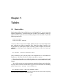
Chapter 1
Stata
Stata is a complete, integrated statistical software package that manages and
analyses data and provides a broad range of sophisticated tools to create attractive summary tables and graphics.Stata 13 adds many new features such as
treatment effects, multilevel GLM, power and sample size, forecasting, effect
sizes, Project Manager, and much more.
This document summarises Stata’s many key features, including its interface, data management and variable manipulation tools and methods for conducting statistical analyses and repeating tasks.
1.1
Interface
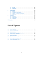
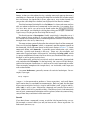
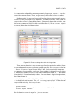
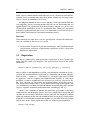
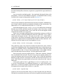
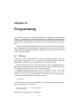
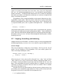
When you open Stata, you’ll see a screen like the one in Figure 1.1. There are
five panes: the Review window, which keeps a list of past commands you’ve
run; the Results window which displays the results of an executed command;
the Variables window which lists variables’ names and labels; the Properties
window which contains meta data on the dataset and its variables; and the
Command window, the prompt in which commands are typed.
There are two ways to input commands into Stata: selecting the command
from a menu at the top of the screen or typing it into the Console at the bottom.
The first option will initially feel most comfortable. This may be the way you
wish to start out using Stata.
However, I recommend migrating very quickly to inputting commands into
the Console. Why? It makes transitioning to programming far easier, since
Stata programming, by and large, involves aggregating many commands into a
single text file. You’ll also save both time finding each command in the menu
bar and energy remembering which sequence of commands you wanted to execute in the first place. The latter reason is particularly compelling for replicating commands – which you will eventually have to do – on the same or even a
different dataset.
However, if you do use the menus, Stata always inputs the corresponding
typed command in the Results window. Jot it down and use the Console next
1
2
CHAPTER 1. STATA
Figure 1.1: Stata’s interface
time.
Customising your view
Stata gives you a small amount of flexibility in customising your view.1 First,
getting rid of the Variables and Properties panes or the Review pane couldn’t
be easier. Simply drag the edge which abuts the Results pane until the window
disappears. You can easily get any pane back again by clicking on, e.g., Window
+ 4 ) in the menu bar.
Variables (
You can change the fonts and display style of Stata’s windows by clicking on
+ , ). Choose the tab of the pane
Preferences General Preferences (
you’d like to customise.
Stata 13.0
1
Increase the size of text in the Results pane to 18. While doing so, notice
that the colour scheme of the Results pane can be changed, and you can
even make your own. The default setting uses a white background and
dark text. My personal favourite is the Mountain scheme, which displays
results in dark green instead of black, making it easier to differentiate
them from commands.
This section is specific to Stata 13 for Mac, although customising your view in Stata works
roughly similarly on a Windows machine and earlier versions of the Mac software. Stata’s Getting
Started Guide (in the PDF documentation which installs with the software – see Section 1.2)
provides exact instructions.
1.2. HELP
3
Preferences are automatically saved when you quit Stata and are reloaded when
relaunched. However, if you rearrange Stata’s windows and alter the fonts and
colours, you can’t revert to any customised settings you had earlier. Get around
this by saving your settings to a named preference set via Stata 13.0 Preferences
Manage Preferences Save Preferences . Any changes you make thereafter do not affect the set; it remains untouched and can be reloaded unless you specifically
overwrite it.
Fool around a bit with the panes until they’re the width you’d
like, then save these preferences. Go back to Stata 13.0 Preferences
Manage Preferences , and you’ll see your newly saved window setup. Click
on it to restore it.
Stata 13.0 Preferences Manage Preferences Factory Window Settings restores the default view. This comes in handy if you’re using Stata on a public machine, and
someone before you already significantly altered the setup.
Current working directory
Look at Figure 1.1. The status bar at the base of the main window contains a
folder path, culminating with the current working directory, that is, the folder
that Stata is “in” – if you tell Stata to save anything this is where it will do
it; should you tell it to open something, here’s where it will look for it. Each
folder in the path is clickable – doing so is an easy way to change the working
directory, handy when you’re trying to find a dataset, do-file, whatever.
1.2
Help
Commands in Stata have syntax, options and prefixes which aren’t always identical. Unless you have a photographic memory, you’re unlikely to remember any
but the most commonly used commands, so don’t even bother. It’s far easier —
and more productive — to familiarise yourself early on with the Stata help files.
With that in mind, let’s make help our first command in Stata. Type the following into the Console:
help
You’ll see links to more information on basics, data management, statistics,
graphics and programming. Click
Basics
Utility commands [ . . .]
Commands everyone should know .2
2
This is true for Stata 12, but Stata 13 now brings up “Advice on finding help” when help
alone is typed in the Console. “Commands everyone should know” can be found in chapter 27 of
the User Guide in Stata 13’s PDF documentation.
4
CHAPTER 1. STATA
This document covers many of the commands listed here, but not all. I have
other hobbies besides writing long, technical documents that few people read.
However, information on every command is readily available each time you
open Stata. Just type help followed by the command of interest. For example,
let’s take a first look at what Stata’s help files have to say about the command
help. Type the following into your Console:
help help
A window pops up with information on the command help. Stata help files
are arranged in a similar order. There’s always a Title section at the top which
states the command. Clicking on the blue-highlighted text — [R] help — loads
the help page in the pdf of the Stata manual. Go ahead, try it3 .
User: Erin HENGEL
The Stata user manual is used even less often than its help file peer, but it includes an absolute wealth of information including extremely detailed descriptions of all commands along with added examples and discussions. The user
guide even starts off with a coherently written sample session. It’s followed by
aTitle
Getting Started Guide, which you’ll find is remarkably similar to this instruction manual. For anyone needing effective bedside reading material, here’s an
[R] help
Display online help
abundant source!
After the title, there’s occasionally information on other relevant commands
or
tutorials. Here, Stata links us to “Advice on getting help”. Take a look at it
Stata's help system
when you get a chance: 99% of learning Stata is just figuring out where to find
There are several kinds of help available to the Stata user. For more information,
the answer.
see Advice on getti
information below is technical details about Stata's help command.
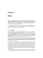
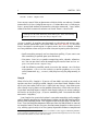
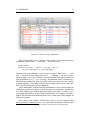
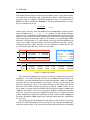
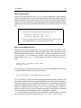
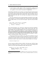
After the brief note on Stata’s help system comes Syntax, which I’ll describe
in more detail in the next section (Section 1.3). Nonetheless, let’s have a brief
look at help’s syntax
Syntax
Display help information in Viewer
Description of commands
help [command_or_topic_name] [, nonew name(viewername) marker(markername)]
Display help information in Results window
chelp [command_or_topic_name]
Syntax of commands
Figure 1.2: Syntax in the help files
Menu
Help
> Stata
Listed
first
is the Command...
syntax for help followed by that for a related command, chelp.
chelp displays help information in the command window. Interesting. To be
3
To load the Stata manual pdf by clicking on links from the help files, you must have Adobe
Description
Reader installed on your machine. For whatever reason, Stata doesn’t realise that other programs,
like
Preview
for Mac,
can also
read
pdf files, soabout
it insists
download
Reader.orIftopic.
you
The
help
command
displays
help
information
the you
specified
command
have a Windows machine, I’m sure Reader came pre-installed with your computer. If you have a
Mac, Stata
you many
download
yourself. and Stata for Windows:
forhave
Mac,toStata
for it
Unix(GUI),
help launches a new Viewer to display help for the specified command or topic. If help is not fol
command or a topic name, Stata launches the Viewer and displays help contents, the table of conten
online help.
Help may be accessed either by selecting Help > Stata Command... and filling in the desired comman
typing help followed by a command or topic name.
chelp will display help in the Results window.
1.2. HELP
5
honest, it does get a bit tedious having a window constantly pop up whenever I
need help on a command. Displaying the help files in the Results window would
be a nice change. Go ahead and try it out: type chelp help in the Console. Do
you get the same help file as before, but displayed in the Results window?
The third section of the help file is called Menu. It’s short and sweet and just
tells you where to find the help command in the menu bar. I’m running Stata
12.1 on a Mac, and it says help can be found under the Help Stata command .
And, sure enough, you should get a dialog box asking you to input a command.
Type in help. Do you get the Stata help-file for help?
The fourth section is Description. Hardly surprisingly, it describes help. I
make a note of always reading it. It’s never too long, and more often than not,
has alerted me to some previously unknown option or function. Go ahead, read
through what it has to say about help.
The next sections generally describe the technical details of the command.
They usually include Options, which, as expected, specifies options specific to
the command. We’ll talk more about in the syntax section (Section 1.3). Some
commands follow with Remarks. It provides more information, tips, tricks
and links. Quickly read through it for help. There are a few examples and
some other suggested topics and materials, including the help guide, which
is a pretty comprehensive tutorial of Stata basics you should meander your way
through as you’re getting used to Stata.
Many commands, particularly statistical analysis commands, also conclude
with some detailed Examples. In the beginning, the syntax will feel foreign,
and hard to interpret. Sometimes, it’s nice to see an actual command in action.
These examples (complete with sample data!) are invaluable, and I hope you
refer to them often.
Last come References, generally sources of statistical techniques. For example, if you type
help regress
(regress is the command to perform a linear regression), and scroll down,
you’ll notice they list two books on econometrics. Both are good, but for those
of you new to empirical analysis, Angrist and Pischke’s work (Angrist and Pischke, 2009) is truly a gem: informative, thorough and actually fun to read (I
know, I didn’t think it was possible, either). They discuss basic, and sometimes
not-so-basic, econometric techniques within a general, often very entertaining,
story of how they used them in their own work.
Search
If you don’t know a command’s name, search for it by keyword using search.
For example, assume I didn’t just tell you how to run a linear regression. To
find out on your own, try
6
CHAPTER 1. STATA
search linear regression
Stata returns several links to documents which it thinks are relevant. Number
two on the list is Stata’s help file on regress. Further down are is a link to gmm,
Stata’s generalised method of moments estimation command. Later, books,
videos even links to external websites are listed. There’s a lot of stuff.
If help can’t find the command you’re looking for, Stata automatically
executes search. Try it out with help regression.
search is useful. It matches your keywords to a database and returns com-
mands, online information and articles from the Stata Journal; it’s basically
Stata’s version of a search engine. It’s pretty smart, but it isn’t Google, so keep
to a few guidelines when using it to make sure you’re getting what you want.4
• Spell everything correctly and use American spelling. If you aren’t sure
how something is spelled, open your dictionary.
• Use nouns. Stata isn’t as good at recognising verbs, adverbs, adjectives,
etc. You can see what I mean by comparing the results from search regression and search regressing.
• Add the following modifier words to restrict the context: data for data
management, statistics for analysis, graph for graphing, utility for
utility commands (e.g., search!) and programming for programming in
Stata.
Google
When all else fails, Google it. If you’re still not 100% sure what you need, or
not clear on what it might be called, Google is your best friend. People ask me
all the time how to do stuff in Stata. Often (but not always), they come to me
after already wasting hours on the problem themselves. Nine times out of ten,
I type their emailed request verbatim into Google and get an answer amongst
the results on the first page. (If you’re wondering how I answered the other
one-tenth – help files).
I use Google a lot, particularly when I want to do something really complex
and I’m hoping someone has already done it before and felt like showing off by
posting their solution online. This happens more than you think. Let me illustrate. I use the World Development Indicators from the World Bank in some of
my empirical work. The data are great, but they come shaped in a rather unusual
way, making typical analysis in Stata pretty impossible without a complicated
4
These guidelines are adapted from Stata’s User Guide. It also suggests additional guidelines
such as using the singular form of a word instead of the plural and being brief, but I’ve never really
found either interfered very much with the results.
1.3. SYNTAX
7
(and tiresome) reshaping. Luckily, others have already figured out exactly how
to do it. By Googling the topic first, I could ride on the coattails of their hard
work. No point in reinventing the wheel.
1.3
Syntax
Let’s talk a bit about syntax. The Stata help files have a pretty good overview
(type help language) and links to more detailed information. Please do check
it out! In fact, just to test your new help skills, have a look at them right now.
You’ll find this page is the source of much of what I’m about to say. In fact, I’m
just going to rip the first line thing I say about syntax straight from it: with few
exceptions, the basic language syntax is
[prefix :] command [varlist] [=exp] [if] [in] [weight] ///
[using filename][, options]
The first time I saw this, I panicked. I don’t speak Greek. In fact, it turned me off
using the help files for about a year. That’s right. For an entire twelve months I
kept a gigantic handwritten list of commands that I had used at some point and
were proven to work. By the end of that first year using Stata, this list was over
100 pages long.
It got to the point that it took me longer to find a command in my list than
figure out the syntax again via trial and error. Since I was using Stata every
day, this was an enormous time suck. So, one morning, I took a deep breath,
launched help language and set out to decode Stata syntax. Ten minutes later
I threw the 100 page handwritten list of commands in the bin.
That’s right. It took me all of ten minutes to learn Stata syntax. Seriously.
It’s that easy. Which is actually terribly irritating: think of how much time I
would have saved had I simply invested 10 minutes upfront? One time, I spent
three hours of my life trying to display a four-way table with means and confidence intervals using survey data. Had I understood the syntax, it would have
been done in three minutes. Three hours of my life gone forever.
Anyway, I hope my little personal story motivates you to familiarise yourself with the syntax. The first thing I want you to note is that anything in square
brackets, [], is optional. Second, notice command. which obviously is a placeholder for an actual command, say, help. This is the only part of the syntax
not in brackets, because it’s usually the only required part of the command. To
illustrate, let’s look again at the help files for help. Under the syntax section,
you’ll see the following description of chelp’s syntax
chelp [command_or_topic_name]
chelp is the only thing required. Because square brackets indicate optional argument, this must mean that one can run the command chelp on its own. Try
it out!
8
CHAPTER 1. STATA
What does command_or_topic_name mean? First, it’s clearly a placeholder
for a command or a topic. Let’s try it out on the only other command we know:
help. Type
chelp help
You should get the help file on help in the Results winder. Now, try it out on
regress. Big surprise: it’s the help file on regress in the Results window.
If you take a look at the syntax for help, you’ll see a bit more “stuff” than
we have for chelp.
help [command_or_topic_name] [, nonew name(viewername) ///
marker(markername)]
help can run on its own, since everything but the actual command is in square
brackets. It’s followed by [command_or_topic_name] as chelp was. What is
that new part, [, nonew name(viewername) marker(markername)]? These
are called options and, because they’re in square brackets (and, uh, because
they’re called options), they are optional. Options are used to turbocharge your
command: they make a plain vanilla a banana split.
Options always come at the end of a command, and a comma must precede
the first option. That comma is very important! It tells Stata that everything
that follows is an option. Stata is stupid. It doesn’t “know what you mean”. If
you leave out the comma, it will think your option is actually part of the regular
command, get confused and throw up an error.
So, what are the options available to the help command? According to the
syntax, there are three: nonew, name(viewername) and marker(markername).
We can find out what they mean by looking at the help file. Check out what it
has to say on nonew:
nonew specifies that a new Viewer window not be opened for the help
topic if a Viewer window is already open. The default is for a new Viewer
window to be opened each time help is typed so that multiple help files
may be viewed at once. nonew causes the help file to be displayed in the
topmost open Viewer.
This option sounds pretty pointless, but let’s try it out, anyway.
help chelp, nonew
What about name(viewername)? What does this command do? How could you
open a help file in a window named Las Vegas? Do it. Can you figure out what the
option marker(markername) does? (Hint: try help regress, marker(Las
Vegas). What happens to the help window you just named Las Vegas?)
1.3. SYNTAX
9
Stata lets you shorten most commands. For example, you don’t actually
need to type help in full. hel or even h works just as well. If you look at the
syntax for help, you’ll see that the first letter is underlined — typing h is the
shortest abbreviation of help that Stata will recognise. If you check out the
syntax for chelp, the first two letters are underlined, meaning Stata recognises
ch as a valid abbreviation but not c. Now, check out the help files for regress.
What’s the shortest legal abbreviation allowed for that command?
When you’re just learning Stata, however, it’s best to type commands out in
full, at least for awhile. You’re learning many new commands, and committing
to memory a word with meaning is probably easier than remembering h brings
up the help files. But, hey, if you want to abbreviate right off the bat, be my
guest.
I’ll explain in more detail what the other parts of the basic language syntax
mean as we encounter more commands that actually use them. For reference,
here are short descriptions of what each are, which you may wish to refer back
to as you are learning Stata (Ródriguez, 2013).
prefix: most commands allow prefix commands, which come before the com-
mand and are followed by a colon. Basically, prefix commands are commands run on commands. There aren’t a lot of them (check out help
prefix to see a full list). The most common are by, svy, capture and
quietly. We’ll talk about by in depth. Check out the help files for information on the other three.
command: this is (usually) the only required element. It denotes the action you
wish Stata to take; hence, it’s almost always an action verb like regress
or summarize. In Stata, the names of commands are lowercase. This is
important, since Stata is case-sensitive! help is a valid command, but
Help, HELP or hElP will just throw up errors (try it!).
varlist: refers to a list of variable names. When varlist follows a command,
then the command is performed only on those variables. Telling a command to restrict itself to varlist is usually optional. Executing a command without varlist following it means the command command is executed on all variables. Like everywhere else in Stata, variable names are
case sensitive.
=exp: means “set equal to algebraic or string expression”. This is used when
generating new variables or replacing the values of existing variables. An
example of an algebraic expression would be log(variable), which says
“take the log of every observation of the variable variable”. A string
expression is just some text in double quotes, e.g. “this is a string expression”.
if: limits the command to only a subset of observations that satisfy some cri-
teria or expression, and is correspondingly called an expression qualifier.
10
CHAPTER 1. STATA
For example, including if variable > 3 tells Stata to execute a command only on those observations that have a value of variable greater
than three.
in: tells the command only to run on a subset of observations that fall within a
range, and is correspondingly called a range qualifier. For example, in 1/
10 tells Stata to execute the command only on the first ten observations.
weight: if your data is weighted, you’ll need to know more about this; check
out the Stata help files (help weights). We won’t bother with it in this
tutorial.
using filename: this is used only when you want to export Stata’s output to
some other file, say myfile.txt. Then, just tack on using myfile.txt and
Stata does it.
options: specified at the very end of the command and preceded by a comma.
Options are command-specific. Different commands take different options. Check out a command’s help files to figure out what they are and
how to include them.
Chapter 2
Data
Stata is pretty useless without data. Since you’re here, I’m sure you already have
a dataset in mind. Nonetheless, when just starting out, you may hesitate to put
it through Training Day. If you’re careful, there’s nothing to worry about —
Stata doesn’t actually make any permanent changes without your explicit sayso. In the interest of public safety however, let’s practice on a sample dataset
that came preinstalled with Stata.
2.1
Loading example data
To see what those sample data files are, type the following command
sysuse dir
sysuse tells Stata you’re interested in the example datasets which came preinstalled with your particular version of Stata; dir asks Stata to list their names.
Those of you familiar with Unix will already recognise dir: it tells Unix to list
the contents of a folder. It has the exact same functionality in Stata.1
For most of this document, we’ll use the auto.dta dataset. Load it up with
the following command:
sysuse auto.dta
Once the data is loaded, you’ll notice that your Variables and Properties windows have changed. For obvious reasons, the Variables window lists the variables in the dataset. The Properties window provides more detailed information
on the variable currently selected in the Variables window. It also has information on the dataset.
1
In fact, dir also works on its own. Test it out to see what it does.
11
12
CHAPTER 2. DATA
2.2
Browsing data
Wouldn’t it be great if you could see the data in a spreadsheet? Surprise, you
can! There are two ways to do this. If you just wish to browse, and not edit, use
the following command
browse
Up pops a spreadsheet of all data currently in Stata’s memory. Click on one of
the data cells. Try to change it. Can’t do it, can you? browse doesn’t let you
alter the data. Luckily, there’s another command, identical to browse in every
way, which does: edit. Type edit in the Console. The exact same spreadsheet
pops up, but now it’s possible to, say, change the price of the 19th observation
to 100,000. Try it. Did it work? Check the Results window. Stata ought to have
responded to your edit by running
replace price = 100000 in 19
Stata then returns a message indicating success: (1 real change made).
Never browse the data in edit mode. It’s too easy to accidentally make
changes. In fact, I never use the edit command for exactly this reason.
I prefer replace, since it’s much more difficult to make an unwanted
modification that way.
2.3
Saving data
Now that you’ve changed the data, let’s save it. This is a sample dataset, which
we’ll want to keep as-is so save it as a new dataset.2 the command for that is
save. Let’s call our dataset new_auto.dta, and save it like so:
save new_auto.dta
Stata saved the dataset in your current working directory, which, if you recall
from Section 1.1, can be found at the bottom of Stata’s main window. Jot it
down, and then navigate to it using your operating system. Is new_auto.dta
there?
With the edit command, change something else in the dataset, e.g., the
price of the 24th observation to 400,000, and save the data again. Did you get
the following error?
file new_auto.dta already exists
2
Stata won’t let us save changes to example datasets, anyway.
2.4. LOADING REAL DATA
13
Why? Because the previous version of new_auto.dta (i.e., the one without the
change to the 24th observation) is already saved under that name. Stata distinguishes between the dataset which you previously saved and the one which is
currently in its working memory. In Stata, you work with a copy of the data, not
the actual data itself. Saving these changes overwrites the original dataset.
In general, you won’t usually save changes to your dataset. Instead, you’ll
want to save the commands you used to make those changes (so you can replicate them) but preserve as much as possible the integrity of the original dataset.
We’ll talk about this more later. For now, let’s assume you really do want to overwrite the earlier version of new_auto.dta. You do so with the replace option
save new_auto.dta, replace
2.4
Loading real data
Verify Stata correctly saved the change made to the 24th observation. To do so,
you’ll first need to clear the data currently in memory and reload new_auto.dta.
The clear command obviously does the job.
As an exercise, use the Stata help files to figure out the syntax clear
needs (hint: it’s really easy). Seriously though, look at the help files. I
know it’s tedious, particularly if you’re the “learning by doing” type. I hear
you. But you also need to learn how to use the help files, so use them.
The command to reload new_auto.dta is use (obviously akin to sysuse):
use new_auto.dta
The data is nicely loaded into Stata’s interface. Check to make sure the changes
you made earlier are there. As a final exercise, reload the original dataset from
the example files. A Chevy Nova should never cost $100,000 and no reasonable
person would pay more than $5,000 for a Ford Fiesta. Adjust their prices.
2.5
Importing data
For many of you, your data isn’t currently in a .dta file. It’s probably in an Excel
file. Everybody’s data is in an Excel file. Raise your hand if it’s an absolute mess
with broken links and disruptive pivot tables. Thought so. Clean it up.
Don’t expect an easy import when you have a monster spreadsheet on your
hands. Stata interprets every cell as a piece of data, so, that total you made
at the end of the last column? Stata thinks it’s another data point: any row
with any kind of character in it (even a space) is interpreted as an additional
observation. Obviously, this could really affect your results; I recommend very
14
CHAPTER 2. DATA
carefully cleaning up your spreadsheet, making sure it contains raw data only
(no sums, weighted averages, whatever), and then export it as a .csv (commaseparated values) file.
Stata can actually import Excel spreadsheets directly. I don’t like to do it
that way, myself: I always get cleaner and more consistent results when
I import a .csv file. Importing Excel files was buggy in earlier versions of
Stata (recent releases work more smoothly). Also, the act of exporting to
.csv gets rid of formatting which is useless (and sometimes confusing) to
Stata and saves data from only one worksheet in a workbook, which is all
Stata can import, anyway.
How do you import the .csv file you just created? There’s a command for that:
import delimited. It grabs a text-delimited file, parses it and imports it into
memory. The original file must have one observation per line, and the values should be separated by a delimiter, e.g., a comma, a semi-colon or basically
anything which forms a boundary between one piece of data and another. Make
sure the first line of your data contains the variable names.
For really complicated imports, you should read Stata’s import help files
(help import). They’re massive, and I’m sure they cover the most obscure import needs. Another option is StatTransfer, external software
which, unfortunately, you’ll have to purchase. It is, however, simple to
use and has always done a fantastic job for me.
So, first thing, let’s take a quick peek at the command’s syntax in the help files.
I’m not kidding, and don’t skip this part.
import delimited [using] filename [, import_delimited_options]
Can you get away with just typing import delimited? No. Why? Because
there’s something that’s not in square brackets namely, filename. And, of
course, that makes total sense. You want Stata to import something. If you
just typed in import delimited, you’re basically saying “Stata, please import”.
Please import what?
using on the other hand, is optional. (Why? It’s in square brackets!) Also
optional are (obviously) import_delimited_options. rowrange(1:500) imports only the first 500 observations; colrange(1:6) imports just the first six
variables.
Anyway, let’s try it. We’ll need some data in .csv form: export the auto.dta
we’re already using as a .csv file, creating a new file, auto.csv, in our working
directory. After that, import it back in again.
2.6. RENAMING DATA
15
export delimited auto.csv
import delimited auto.csv
The import didn’t work, did it? Stata can only handle one dataset at a time,
and you already have one loaded. We learned in Section 2.4 to use clear first.
There’s actually an even easier way: tack clear onto import delimited as an
option, accomplishing everything in one step.
import delimited auto.csv, clear
Have you successfully imported the data? Good. Let’s play with a few options.
What if you only wanted to import the second through fifth variables?
import delimited auto.csv, clear colrange(2:5)
The notation 2:5 tells Stata to start importing at the second variable and end
at the fifth. What about importing only observations 20-300? Use rowrange().
import delimited auto.csv, clear rowrange(20:300)
2.6
Renaming data
Suppose you find the free market an oppressive capitalist construct and you
wish to rename price to reflect this. Fine. Whatever. We’ll use the rename
command for that:
rename price oppressive_cap_construct
Congratulations. You’ve renamed a variable. Now, take a moment to browse
the help files for rename. Does the command you just typed mimic the correct
syntax? While you’re at it, attempt a few of the examples Stata gives.
A few notes on naming variables. It’s good early on to establish some
sort of consistent naming convention. If you’re interested, here are a few
guidelines I tend to keep.
1. First, I like my variable names short. Although names can be
as long as 32 characters, the Variable window only shows the
first few. This is annoying when you have more than one variables starting alike — e.g., price_constantinople_1891 and
price_constantinople_1892. Short names are also faster:
typing thisisaninsanelylongvariablename gets old, fast.
16
CHAPTER 2. DATA
2. Second, I use lowercase. Stata is case-sensitive, so myVar and myvar are two different variables. If I don’t use all lowercase, then I
forget which letter I capitalised. Lowercase also obviates the need
to hit the shift key, which saves time and energy, but that may be
going overboard. Anyway, there are pluses and minuses to using all
lowercase (or all uppercase) or a combination. Lowercase is just my
personal preference.
3. Third, variable names must start with either a letter or an underscore (_), but may contain numbers (and letters and underscores)
thereafter. Names cannot begin with a number and forget about
including special characters like %, & and #.
Pop quiz. Which of the following variable names are legit: ghetto, 1superstar, _that_is, Wh@tUR, afar4353?
Exercises
This exercise is from the Stata help files for rename. An answer for this exercise
is available in the exercises.do file.
1. Load the dataset renamexmpl.dta from the web. Change the names of
exp to experience and inc to income. Describe the data to make sure
the name changes have been made.
2.7
Labelling data
There are numerous ways to label data in Stata. The first way, and the one you’ll
use most often, is to label variables. You can see variable labels directly in the
Variable window: just to the right of the variables themselves.
To define or change a variable’s label, use the label variable command
followed first by the name of the variable and then by the desired label, in double
quotes (single quotes will not work). If you wish to relabel the variable trunk
from “trunk space (cu ft.)” to “boot space (cu ft.)”, you’d type:
label variable trunk "boot space (cu ft.)"
You can also attach notes to specific variables via the notes command. I use
notes to store sources, methodology and any other random information I’m
loathe to forget. Since variable labels hold up to 80 characters (actually, I keep
them even shorter to make pretty labels on tables and charts — more on this
later (Section 5.2)), I save extraneous information with notes All The Time.
The syntax for notes differs from that for adding labels. Check out the syntax
in the help files: notes evarname: note. Do you see how to add the note “cu.
ft. refers to cubic feet” to the variable trunk? Like so.
2.7. LABELLING DATA
17
notes trunk: cu. ft. refers to cubic feet
Verify the note was made in the Properties window, making sure trunk is highlighted in the Variable window (you may need to click on the plus sign next to
Notes to expand it). You can actually add multiple notes to each variable: one
note for the source and another which mentions the methodology. To list the
notes associated to trunk, execute
char list trunk[]
(What happens if you omit trunk[]?) You’re probably wondering where char
came from. It stands for characteristics. A dataset and its variables have associated with them a set of characteristics, and notes are considered characteristics.
Hence, char must be called to list them. And, no, labels are not characteristics.
The only good practice I can give you for labelling your variables is to
do it early and do it often. I label my variables with as much detail as I
can as soon as I create them and change the labels whenever I change the
variable values (e.g., if I log a variable). This is a pain, and you won’t want
to do it. You’ll think “Oh, I’ll definitely remember what var34523 refers
to in three years time”. So you won’t label your variables. And then, three
years later, when you desperately need to rerun your results and the fate
of the universe is depending on knowing what var34523 actually is, you
won’t know. Unfortunately, this is one of those lessons you can only grasp
the hard way. So, while I recommend you assiduously label variables, I
know my advice will go unheeded. Sigh.
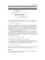
Besides labelling variables, you should also label their values. Consider the
categorical variable: foreign. Peruse it. You’ll see that foreign has numerical
values, but there are labels assigned to each value: 1 means a car is foreign; 0
means it’s domestic. To list all the value labels in a dataset, use
label list
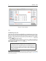
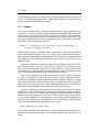
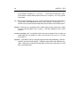
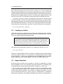
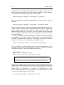
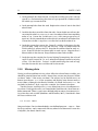
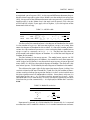
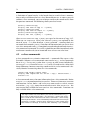
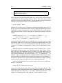
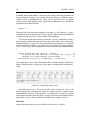
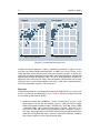
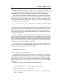
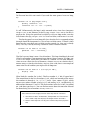
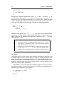
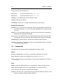
Our dataset has only one defined value label. It’s called origin. Type codebook
foreign and you’ll see origin is associated to foreign. It’s a bit difficult to
find, so pointed it out in the graphic below.
Stata has a two-step approach to setting value labels: first define, then assign. Let’s use it to define labels for rep78. Step one, define a set of labels.
origin is the set of labels assigning 1 to Foreign and 0 to Domestic. rep78
has five distinct values. Let’s create the set of labels repairs to describe each
of these five values.. Assuming a low value of rep78 is good, our set of labels
might look something like this
label define repairs 1 "Excellent" 2 "Strong" 3 "Okay" ///
4 "Poor" 5 "Weak"
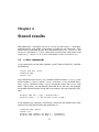
r(602);
17 . log using "/Users/erinhengel/Desktop/Untitled.smcl", replace
name:
log:
log type:
18opened on:
<unnamed>
/Users/erinhengel/Desktop/Untitled.smcl
smcl
24 Mar 2013, 00:52:54
CHAPTER 2. DATA
18 . codebook foreign
foreign
Car type
type:
label:
numeric (byte)
origin Name of the value
range:
unique values:
[0,1]
2
tabulation:
Freq.
52
22
19 .
label definition
Numeric
0
1
units:
missing .:
1
0/74
Label
Summary of the
Domestic value labels
Foreign
Figure 2.1: Label definitions
Step two, associate the label definition repairs with rep78. Use the label
values command, much as we earlier used the label variable command:
label values rep78 repairs
(Take a peek at the help files to make sure we got the syntax right.) Browse the
variables. Does rep78 show
blue?
how
Sunday,up
24 in
March
2013(Recall
00:55 Page
22 to do this? Check out the
section on viewing data (Section 2.2)). If it does, drumroll please, you’ve successfully added a label. You can, and, in fact, should, assign one label definition
to several variables. For example, if you had rep79, the repair record in 1979,
you could also assign the value label repairs to it.
You can label your entire dataset in much the same way you label individual variables: just type label followed by data and your chosen label, again in
double quotes. That’s it. Right now, if we check out the Properties window, we
see that the dataset is labelled 1978 Automobile Data. Let’s change the label
to 1492 Santa Maria Data:
label data "1492 Santa Maria Data"
Check your Properties window. Does it reflect the change?
Adding notes to your dataset is almost identical to adding notes to a particular variable. Just type notes: followed by the text of the note you wish to add
(again, without double quotes). Let’s label our dataset as follows:
notes: Roswell Files, FBI
The new note is in the Data panel of the Properties window. You may need to
expand the Notes section (again, click on the plus sign to the right).
Exercises
These exercises are from the Stata help files for label. Answers for these exercises are available in the exercises.do file.
2.8. ORDERING DATA
19
1. Load hbp4.dta from the web. Label the dataset “fictional blood pressure
data”.
2. Label the hbp variable “high blood pressure”.
3. Define the value label yesno.
4. List the names and contents of all value labels.
5. List the name and contents of only the value label yesno.
6. Make a copy of the value label yesno.
7. Add another value, 2, and label, maybe, to the value label yesno. Rename
it yesnomaybe.
8. List the name and contents of the value label yesnomaybe.
9. Modify the label for the value 2 in value label yesnomaybe.
10. List the name and contents of value label yesnomaybe.
11. Attach the value label yesnomaybe to the variable hbp.
12. Drop the value label sexlbl from the dataset.
2.8
Ordering data
Let’s start with ordering variables. Note the order of the variables in the Variable window. The first variable is make What if you wanted the variable price
first? Well, you might try dragging and dropping variables in the Variable window, but that’s fruitless. For whatever reason, the Stata developers haven’t yet
realised that this is the intuitive way to reorder variables. Fine. Luckily, it’s not
hard. Just type order followed by the variable (or variables) you wish to put at
the top, and then , first (note the comma before first), that is
order price, first
and lo and behold, price jumps to the front of the queue. If you wanted price
at the end, type
order price, last
order actually has a number of options that allow you to do all kinds of crazy
things to the order of your variables. Besides simply putting variables at the
top or the bottom of the list, one can also tell Stata to put, say, price before
turn or after rep78. You can even tell Stata to place the variables in alphabetic
order. As always, check out the help files!
20
CHAPTER 2. DATA
What if you wanted to sort the observations in, say, ascending order? sort
has you covered. Let’s try it out with the single variable price. First, browse
observations one through ten of price. Next, execute sort price, and browse
again. Not the same, are they?
One can also sort based on two or more variables. Execute sort foreign
price. All domestic cars are at the top; they are then ordered according to price.
All foreign cars come next, and they, too, are then in ascending order. String
variables are sorted, as one would expect, alphabetically. Test it out with sort
make.
Exercises
These exercises are from the Stata help files for order and sort. Answers for
these exercises are available in the exercises.do file.
1. Move make and mpg to the beginning of the dataset.
2. Make length the last variable in the dataset.
3. Make weight the third variable in the dataset.
4. Alphabetise the variables.
5. Arrange observations into ascending order based on the values of mpg.
6. List the 5 cars with the lowest mpg.
7. List the 5 cars with the highest mpg.
8. Arrange observations into ascending order based on the values of mpg,
and within each mpg category, arrange observations into ascending order
based on the values of weight.
9. List the 8 cars with the lowest mpg, and within each mpg category, those
cars with the lowest weight.
2.9
Creating data
generate is the go-to command for creating new variables. Let’s illustrate
with an example. Assume it’s really important to calculate the price-to-weight
ratio. I have no idea why one would need this statistic, but the world is full of
things I don’t understand. I deal with it. So I’ll create it and call it p2w:
generate p2w = price / weight
And, that’s it. In general, generate is followed first by the name of the new
variable you wish to create, then the equal sign, =, and ends with a data transformation which defines the new variable. Again, check out the help files. Is it
possible to assign value labels when creating variables?
2.9. CREATING DATA
21
What if you want to create a new dummy variable, equal to one if rep78 is
greater than 3 and zero otherwise? The syntax is the same as before, but you
add an if-qualifier at the end, like so
generate klunker = 0
replace klunker = 1 if rep78 > 3
This gives you the new variable klunker equal to one if the car needs to be
repaired more than three times a year, and zero otherwise. (Yes, I misspelled
klunker; it’s actually clunker; whoops! But, I can’t be bothered to change all of
the graphics, so I’m just letting the mistake stand. Sorry!)
Notice also how I surreptitiously snuck in the replace command. replace
modifies a variable. Its syntax is identical to that for generate. The only
difference, obviously, is that, while generate tells Stata to create a brand new
variable, replace tells Stata to replace the values of an already existing variable
with something else.
The if-qualifier at the end of the replace command is a logical expression:
it tells Stata to only replace the value of klunker with a 1 if the car has a high
repair record, i.e., rep78 > 3.
To get rid of a variable, use drop like so
drop klunker
and poof, it’s gone. Be careful, though! It’s gone forever, and Stata doesn’t give
you any helpful messages like “Are you sure you really want to do that?”.
Now is a good time to introduce another qualifier: the in-qualifier. Assume
you wanted to drop the first observation. You’d type
drop in 1
Browse the data. Is the first observation gone? What if you wanted to drop the
first ten observations? See the help files for in to show you how. After you’re
done, reload the dataset with
sysuse auto.dta, clear
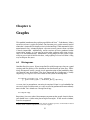
I now want to show you an even easier way to create klunker that uses a little
trick:
generate klunker = rep78 > 3
This one line generates exactly the same variable klunker that we created earlier. Stata evaluates the statement rep78 > 3 for each observation, and it returns true or false. Since the numerical value of true is one and false is zero (this
22
CHAPTER 2. DATA
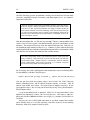
is a convention adopted by most programming languages), rep78 > 3 evaluates either to one or zero. Thus, you get exactly the same klunker as before.
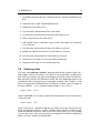
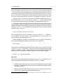
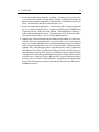
Unfortunately, I’m sorry to have to tell you that the way we created klunker
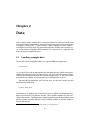
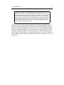
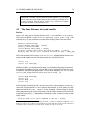
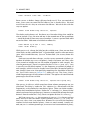
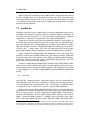
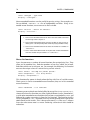
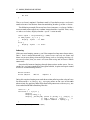
in the last few paragraphs was incorrect. To understand why, take a look at
rep78 and klunker in spreadsheet form. (To see only these two variables, use
the browse command and list both variables after it, like so: browse rep78
klunker.) Note the third observation:
Figure 2.2: Errors creating data with missing values
That . means there isn’t any data on rep78 for that particular vehicle. Since
klunker depends only on rep78, we would naturally wish klunker to also be
.. But no. klunker is equal to one! Why? Well, Stata technically interprets .
as some very large number, and a very large number is obviously greater than
1, hence Stata codes klunker as one when it should be coded as .. What does
Stata do this? I have absolutely no idea. I’m sure there’s a logical explanation,
but I don’t know it.
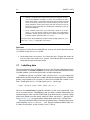
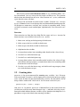
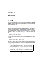
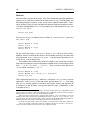
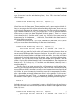
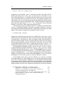
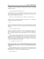
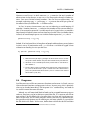
Luckily, it’s easy to fix: add the if-qualifier if !missing(rep78) at the end.
! is the logical not operator. Thus, if !missing(rep78) says “if the value of
rep78 is not missing”. Let’s try this out:
drop klunker
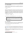
generate klunker = rep78 > 3 if !missing(rep78)
browse rep78 klunker
Ba-da-boom! klunker is equal to ., just as we want.
2.9. CREATING DATA
23
Figure 2.3: The missing() expression
What if we wanted klunker to have more nuance? Say we wanted it equal
to one only if both rep78 > 3 and mpg < 20 are true. Easy.
drop klunker
generate klunker = (rep78 > 3 & mpg < 20) ///
if(!missing(rep78) & !missing(mpg))
Here we have a new operator: &: for klunker to equal 1, both rep78 > 3 and
mpg < 20 must be true. Note that rep78 > 3 and mpg < 20 are in parentheses as both !missing(). Neither sets of parentheses are actually necessary
(the parentheses in, e.g., !missing(mpg), on the other hand, are necessary).
You could leave them off. They just make it clear to us humans what is being
grouped together. I find they make the line of code a bit easier to read. But
that’s just one of my own stylistic adoptions.
A final command I’d like to turn your attention to is egen, which stands for
extensions to generate in that it extends the generate command3 . Technically,
egen does nothing you couldn’t otherwise achieve with generate and replace.
It just does them better. It has a lot of functionality, and I suggest you take a
look at the help files for a full description. But I’ll show you a few examples to
illustrate its power.
First, what if you wanted a variable mean_mpg_by_foreign equal to the
mean of mpg of a subgroup of cars, say, those that are foreign and those that
3
This section is based on material from the blog the Stata-Project-Oriented-Guide.
24
CHAPTER 2. DATA
are domestic? I’m sure you could easily do this with generate and replace,
but it would take more than a few lines of code to achieve it. If you use egen,
instead, you can accomplish everything in one step with
egen mean_mpg_by_foreign = mean(mpg), by(foreign)
If you wanted the mean of subsets determined by foreign and rep78, egen can
handle it.
egen mean_mpg_by_foreign = mean(mpg), by(foreign rep78)
One isn’t limited to means, either. egen supports a number of functions. For example, rowmean() calculate the average of number of variables. Coupled with
the by() option, you’ll get group specific averages of several variables. This
could be useful if you have, say, rep78, rep79 and rep80, and you wanted to
create a variable to hold their average over subgroups of cars determined by
foreign and rep78.
total() creates a constant containing the sum of the variable (or variables)
in parentheses. On it’s own, I think it’s rather useless, but when used with the
by option, it becomes more attractive. For example, it can create a total of
rep78 for all foreign cars and another for all domestic, like so
egen tot_rep78_by_foreign = total(rep78) by(foreign)
total(), like mean(), treats missing values as zero. If the option missing is
specified, however, then if all observations are missing, all values in the new
variable are missing, as we can see when we do just that
generate missing = .
egen tot_zer = total(missing)
egen tot_missing = total(missing), missing
Distinguish carefully between Stata’s sum() function and egen’s total() function. Stata’s sum() function creates the running sum, whereas
egen’s total() function creates a constant equal to the overall sum.
The group() function takes a list of variables (usually categorical) and assigns a
number to each distinct group those variables make. For example, rep78 takes
on five values. foreign takes on two. There are therefore ten possible subgroups: rep78 == 1 and foreign == 0, rep78 == 1 and foreign == 1, etc.
It’d be rather tedious to create a variable like that using simply generate and
replace, but it couldn’t be easier with egen.
egen grp_rep_foreign = group(rep78 foreign)
2.9. CREATING DATA
25
If you investigate, you’ll note that egen actually only created eight categories
— turns out their aren’t any foreign cars with repair records of one or two. In
this example, egen ignores missing values in rep78: anytime rep78 isn’t there,
grp_rep_foreign is also missing. If you’d like egen to treat the missing values
in rep78 as their own category, use the missing option. Go ahead: try it out!
Anyway, egen is a time-saver, and very, very flexible. Other functions you
can use with it are min(), max(), median(), mode(), . . .. The list seriously goes
on. Check out the help files for more information and loads of examples.
Three more time-savers are tablulate with the generate option for creating dummy variables, encode for converting string variables into numbers
labeled with those strings and recode to create categorical variables. I discuss
recode in Section 5.2. Try the following example to see how to create dummy
variables using tabulate:
tabulate rep78, generate(repairs)
Stata created five new dummy variables, repairs1, repairs2, . . . where repairs1 equals 1 if rep78 equals 1 and zero otherwise, repairs2 equals 1 if
rep78 equals 2 and zero otherwise, etc.
Often, categorical variables save their information as strings. To see what I
mean, load the hbp2.dta example dataset from Stata’s website:4
webuse hbp2
browse the data and note that the variable sex stores its two values “male” and
“female” as strings. To perform a regression analysis controlling for gender
requires a numeric variable. encode handles this, even properly labelling the
numeric variable it generates with the strings from the original variable:
encode sex, generate(gender)
Exercises
These exercises are from the Stata help files for generate, drop and egen. Answers for these exercises are available in the exercises.do file.
1. Load genxmpl3.dta from the web. Create the variable age2 with a storage
type of int and containing the values of age. Replace the values in age2
with those of ageˆ2.
2. Load genxmpl2.dta from the web. List the name variable. Create the variable lastname containing the second word of name.
4
To load datasets from the Stata website use webuse. It functions very similarly to sysuse.
See the help files for more information.
26
CHAPTER 2. DATA
3. Load genxmpl3.dta from the web. Create the variable age2 with a storage
type of int and containing the values of age squared for all observations
for which age is more than 30.
4. Load genxmpl4.dta from the web. Replace the value of odd in the third
observation.
5. Load the database stan2.dta from the web. Create duplicates of every observation for which transplant is true. Sort observations into ascending
order of id. Create the variable posttran, with storage type of byte,
equal to 1 for the second observation of each id and equal to 0 otherwise.
Create the variable t1 equal to stime for the last observation of id.
6. Load the system data census.dta. Drop all variables with names that begin with pop. Drop marriage and divorce. Drop any observation for
which medage is greater than 32. Drop the first observation for each region. Drop all but the last observation in each region. Keep the first 2
observations in the dataset. Drop all observations and variables.
7. Load the auto.dta sample data.Create highrep78 containing the value of
rep78 if rep78 is equal to 3, 4, or 5, otherwise highrep78 contains missing
values. List the results. Create a variable containing the ranks of mpg.
Sort the data on this new variable and list the results
2.10
Missing data
Having just discussed how missing values affect the value of new variables, you
should be worried about how much a threat they are you your dataset. Where
are these “holes”? How many are there? The easiest way to find this out is to
browse your dataset. list is also an option, and displays your dataset much as
browse does, although in the Results window. Go ahead and try out list. See
any holes in the data? Yeah, rep78 has a couple. Let’s home in on them.
For this dataset, scrolling with list was enough to give us a handle on missing values. For bigger datasets, we’ll need either patience and a lot of time or a
better command. There’s a great user-defined program mdesc that counts missing values for each variable (Medeiros and Blancette, 2013). Download it from
the Stata archives with
ssc install mdesc
Congratulations! You just downloaded a user-defined program — mdesc — from
the Stata archives. mdesc now works like any other Stata command. It even has
a help file! (Go ahead, check it out.)
2.10. MISSING DATA
27
There are a wealth of user-defined programs out there for Stata — and
I use quite a few in my day-to-day work. You should too. To see the list
of all user-defined packages you’ve already installed, type ado dir in
the Console. To uninstall any of them, type ado uninstall PROGRAM
where you obviously replace the word PROGRAM for the name of whatever
actual program you wish to uninstall. (UCLA Institute for Digital Research
and Education, 2013) Go ahead, try it: uninstall mdesc. But then install it
again, because we’re about to use it.
Right. Let’s use this new command mdesc that we just installed ourselves. It
couldn’t be easier. Just type mdesc into the Console. You should get a table listing each variable, the number of missing values it’s missing and the percentage
they are of total observations. rep78 has five missing values: about 7% of observations. No other variable has any missing data. Frankly, for most datasets,
this is about all you need to get a handle on missing values; but, if you ever
want a better overview of their patterns and distribution, check out this FAQ
from UCLA.
Chapter 3
Analysis
3.1
Mean
The summarize command gives a good overview of a variable’s basic statistical
properties. To use it, type summarize followed by the variable (or variables) of
interest. For example, with
summarize price mpg
you’ll get a table containing the number of observations, the mean, the standard deviation, the minimum and the maximum of price and mpg in the Results
window. If you want more detail, such as percentiles (including the median —
i.e., the 50th percentile), variance, skewness and kurtosis, add , detail (note
the comma — detail is an option — see Section 1.3) after your variables, like
so
summarize price mpg, detail
If you only need summary statistics on price and mpg for foreign cars, add an
if-qualifier.
summarize price mpg if foreign == 1
Your table, of course, differs a bit from the earlier table. The means of both
price and mpg are slightly higher — foreign cars are more expensive and have
better gas mileage.
What’s the difference between = and ==? The = sign tells Stata to set
a variable equal to something. It is used to actually change the value of
a variable in the generate and replace commands. The == sign, on
the other hand, is a logical operator: it tells Stata to test a statement to
see if it is true. For example, Stata interprets 1==2 as “Is 1 equal to 2?”.
It obviously isn’t, so Stata returns false, i.e. 0. If, however, the statement
29
30
CHAPTER 3. ANALYSIS
read 1==1, Stata sees “Is 1 equal to 1?”, which is true, so Stata returns
true, i.e. 1.
Actually, now that I’m at it, how did I know that foreign == 1 if the car
is an import? First, recall that the numerical value of true is one. Thus,
since the variable is called “foreign”, one would assume that foreign
== 1 is true for cars that are, indeed, foreign. However, it’s never a good
idea to assume your fellow man is logical. Always double check with the
codebook command. Typing codebook foreign into the Console returns information on the values and value labels associated to the variable
foreign. Try it out. Does zero corresponds to Domestic and one to Foreign? It should.
Another neat way to disaggregate summary statistics uses by. by is a prefix command, which we talked about in Section 1.3. For certain commands, including
summarize, you can place by varlist: (recall, varlist refers to a list of variables, e.g., foreign rep78 price) before you run the command. Let’s try it:
by foreign: summarize price mpg
Thus, Stata runs summarize first on the subset of domestic cars (i.e., foreign
== 0), and then the subset of foreign cars (i.e., foreign == 1). How could you
use summarize with an if-qualifier at the end to achieve the same results?
The command mean is used in much the same way as summarize, although
it obviously only provides information on the mean of a particular variable (including its standard error and 95% confidence interval). Let’s test it out with
price and mpg
mean price mpg
Again, should you wish to restrict the data to only a subset you can use an ifqualifier exactly as we used it with summarize. Unfortunately, however, the by
command won’t work with mean (by works with most commands, but not all).
mean does come equipped with the over option, which does the same thing
mean price mpg, over(foreign)
I have no idea why by works with summarize but not with mean and why over
works with mean but not summarize. One of those quirks of Stata, I suppose.
Exercises
These exercises are from Stata’s summarize and mean help files. Answers for
these exercises are available in the exercises.do file.
3.2. CORRELATION
31
1. Load fuel.dta from the web. Estimate the average mileage of the cars without the fuel treatment (mpg1) and those with the fuel treatment (mpg2).
2. Load highschool.dta from the web. Estimate a population mean using survey data.
3. Estimate the mean of weight for each subpopulation identified by sex.
4. Load auto.dta. For each category of foreign, display summary statistics
for rep78.
5. For each category of rep78 within categories of foreign, display summary statistics.
3.2
Correlation
What about correlation? That is, to what degree are, say, price, mpg and rep78
correlated? For that we have two different commands: correlate and pwcorr
(pwcorr stands for pairwise correlation). Both are used in exactly the same way.
They only differ (and then only slightly) in how each calculates the correlation
matrix. correlate uses only those observations which have no missing values
in any of the variables of interest; pwcorr, on the other hand, uses as many
observations as it can to calculate each pair-wise correlation statistic.
This may be easier to understand with an example. Recall that rep78 has
a few missing values (type browse rep78 to verify). Let’s see how correlate
and pwcorr are affected by these missing values.
correlate price mpg rep78
pwcorr price mpg rep78
The correlations between mpg and rep78 and price and rep78 are identical
in both tables. This is because correlate and pwcorr use the same observations to calculate the correlations. However, the correlation between price and
mpg is –0.4559 in the first table, but –0.4686 in the second. Why? correlate
omits all observations where rep78 is missing, even when it’s only calculating
the correlation between price and mpg. pwcorr, on the other hand, cares only
whether observations of price or mpg are missing when calculating their pairwise correlation. It couldn’t care less if any values of rep78 are missing. Use
correlate to run the correlation matrix only on price and mpg. Does this correlation value correspond to what we got earlier using correlate or pwcorr on
all three variables? Why do you think that is?
Should you use correlate or pwcorr? If you don’t have a large number
of missing values in your data, then it doesn’t really matter. However, since
pwcorr uses at least as many observations as correlate to it to calculate its
correlation matrix, it produces more accurate pairwise results. On the other
32
CHAPTER 3. ANALYSIS
hand, regress deletes observations like correlate, so you may wish the correlation matrix to include only those data points without any missing values.
Also, it’s easier to remember correlate.
An additional benefit of pwcorr are its options, which you should check out
in its help files. pwcorr has more options than correlate, for example the sig
option displays the significance level for each entry and the star(0.05) stars
all correlation coefficients at the 5% significance level. There isn’t any option
to display significance levels for correlate. Nonetheless, I still use correlate
pretty often, if only because I can never remember pwcorr.
Exercises
These exercises are from Stata’s correlate help files. Answers for these exercises are available in the exercises.do file.
1. Load auto.dta. Estimate all pairwise correlations. Add significance levels
to each entry. Add stars to correlations significant at the 1% level after
Bonferroni adjustment.
3.3
Regression
The regress command is used to run linear regressions in Stata. Do the right
thing and take a look at its help files. The syntax mirrors many of our earlier
commands.
regress depvar [indepvars] [if] [in] [weight] [, options]
depvar refers to the dependent variable, also sometimes referred to as the y
variable, left-hand variable or regressand. It’s affected by one or more independent variables — indepvars — also known as x variables, right-hand variables
or regressors. regress supports the (hopefully now familiar) if- and rangequalifiers (if and in, respectively) just as generate, replace, summarize, etc.
do. Thus, you may run regressions on restricted subsets of the data that either satisfy some criteria (use if) or are within some range of data points (use
in). Additionally, just below the table of options in the help files you’ll see that
regress supports numerous prefix commands, including by and svy.
regress has a number of options for specifying your model, calculating
standard errors and displaying results. Let’s run a simple linear regression and
see how we can use them. Recall that weight measures the weight of a vehicle
while mpg accounts for the average number of miles it can go on a single gallon
of petrol. It’s reasonable to expect that lighter cars get more miles to a gallon;
heavier cars, fewer. Linear regression is one way of testing this hypothesis.
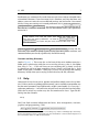
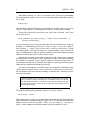
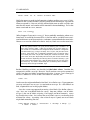
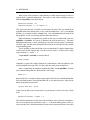
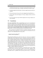
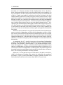
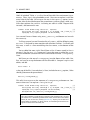
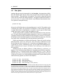
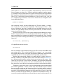
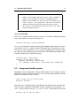
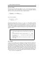
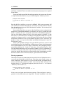
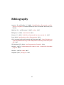
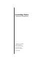
regress mpg weight
3.3. REGRESSION
33
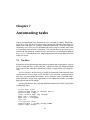
You should receive output in the Results window similar to the figure below.
Let’s look first at the lower table, highlighted in yellow. According to the regression, weight is indeed a significant predictor of mpg: it’s standard error is
User: Erin HENGEL
0.0005179 and its coefficient –0.0060087. Dividing the coefficient on weight
by its standard error we get
Residual
851.469256
−0.0060087
= −11.60
0.0005179
72 11.8259619
R-squared
= 0.6515
Adj R-squared = 0.6467
independent variable, the deRoot MSE
= 3.4389
which is the t-statistic. Since the model has one
Total
2443.45946
73 33.4720474
grees of freedom are N − p = (74 − 2 = 73, where N is the number of observations and p is the number of parameters (the coefficient on weight plus the
constant).mpg
You couldCoef.
have also
found
inP>|t|
the smaller
in Interval]
the upper
Std.
Err.this figure
t
[95%table
Conf.
right hand corner of the output under df. Assuming we’ve specified the model
wt000
-11.60assure
0.000
-7.041058
-4.976316
correctly,
a quick-6.008687
glance at a.5178782
t-table should
you that
the coefficient
on
_cons
39.44028
1.614003
24.44
0.000
36.22283
42.65774
weight has a 100% chance of being statistically different from zero. There’s
no need to refer to t-tables, however, as Stata calculates it automatically: the
comes
right after the t-statistic in the table.
8 p-value
. regress
mpg weight
Source
9 .
SS
df
MS
Model
Residual
1591.9902
851.469256
1
72
1591.9902
11.8259619
Total
2443.45946
73
33.4720474
mpg
Coef.
weight
_cons
-.0060087
39.44028
Std. Err.
.0005179
1.614003
t
-11.60
24.44
Number of obs
F( 1,
72)
Prob > F
R-squared
Adj R-squared
Root MSE
P>|t|
0.000
0.000
=
=
=
=
=
=
74
134.62
0.0000
0.6515
0.6467
3.4389
[95% Conf. Interval]
-.0070411
36.22283
-.0049763
42.65774
Figure 3.1: Regression output
The value of the coefficient on weight is negative, supporting our original
hypothesis. The right-hand side lists the 95% confidence interval band. We
can be 95% sure that the coefficient on weight lies between –0.007 and –0.005.
Note that the unit of measurements for weight and mpg are one pound and
one mile, respectively. Thus, a one pound increase in the weight of a vehicle
decreases the number of miles one gets per gallon by –0.006. Since cars are
heavy items, it’s more natural to think of increasing their weight in 100 or even
1,000 lbs. increments. To do so, just multiply –0.006 by whichever increment
you wish: increasing weight by 1,000 means one will get six fewer miles per
gallon. Another way to do this would be by creating a new variable wt000 equal
to weight divided by 1,000. Regressing it on mpg should give you a coefficient
of –6 (Try it!).
The table upper left (highlighted in red above) is the analysis of variance,
or ANOVA, table. The columns are sum of squares (SS), degrees of freedom (df)
and mean squares (MS). The first cell of the first column computes the model
34
CHAPTER 3. ANALYSIS
or explained sum of squares (ESS): its the squared difference between the predicted value of mpg and its mean value. Below it are the residual sum of squares
(RSS): the squares of the difference between what mpg actually is and what the
model predicts it to be. Below that is the total sum of squares (TSS): the sum
of ESS and RSS, which, if you apply a bit of algebra, is just the squares of the
demeaned values of mpg.
Table 3.1: ANOVA table
Source
Model
Error
Total
SS
Pn
ESS = i=1 (ŷi − ȳ)2
Pn
RSS = i=1 (yi − ŷi )2
Pn
TSS = ESS + RSS = i=1 (yi − ȳ)2
df
MS
nβ
N =ε−p
nT = nβ + nε
ESS
nβ
MSE =
TSS
nT
RSS
p
The first cell of the second column is the degrees of freedom for the model:
it’s the number of regressors. We have one regressor, weight, so it’s one. Next
comes the degrees of freedom for the residuals. It’s the total number of observations less the number of parameters: we’re estimating both a coefficient on
weight as well as a constant, so it’s 74 − 2 = 72. The total row lists the sum
of the model and residual degrees of freedom. It’s called the total degrees of
freedom for the model.
The final column is the mean squares. The model mean squares are ESS
divided by the model degrees of freedom. Our model has only one regressor,
so MS is equal to ESS. Below it are the residual mean squares, or mean squared
errors (MSE). It’s RSS less the residual degrees of freedom. The final cell is the
total mean squares: TSS divided by the total degrees of freedom in the model.
The table on the upper right of the regression output figure (in blue) lists
statistics related to the overall model fit. Listed first are the number of observations used to calculate the regression. Below it is the F-statistic which tests
the joint significance of all independent variables. Since there’s only one, it’s
equivalent to the t-test — it’s just the t-statistic squared (try it out!). Again,
you could look at an F-table to see if 134.62 is statistically significant, but Stata
calculates the p-value automatically — it’s displayed just below the F-statistic:
0.000.
Table 3.2: Model fit statistics
Statistic
Number of observations
F (nβ , nε )
R2
R̄2
Root MSE
Definition
N
MSM
M SE
ESS
TSS
n
β
R2 − (1 − R2 ) N −p
√
MSE
Next comes R-squared. It is ESS divided by TSS. Historically, R2 is assumed
to reflect how well a model fits the data. It’s a number between zero and one:
3.3. REGRESSION
35
the closer R2 is the one, the better the fit. Unfortunately it has a few drawbacks, the biggest of which is that it actually suffers from its own simplicity. It’s
easy to interpret. You don’t need much statistical training to understand that
a high R2 is good: your model is explaining a lot of the variation in the data!
You do, however, need at least some statistical training to realise that it’s only
good if your model is correctly specified. High R2 s may erroneously arise from
omitted variables, mis-specifying the functional form, and most overlooked of
all, from having too many regressors, since increasing the number of explanatory variables always increases (or, in rare cases, doesn’t decrease) the R2 . Misspecifying the functional form and omitted variables affect all regression statistics; they, however, are slightly more difficult to interpret and won’t “improve”
as you recklessly add more right-hand variables (in fact, they’ll probably get
worse). So, it’s less of a risk that one will draw quick and superficial conclusions
from them.
Moreover, micro-economists are generally interested in the relationship between a particular independent variable and the dependent variable; usually,
they are less interested in how well the overall model explains the data. Instead,
they care about correctly specifying the model’s functional form and including
appropriate controls so as to reduce bias on the regressor of interest. Macroeconomists, who often attempt to predict an outcome, are more concerned with
the statistic.
As mentioned, the R2 is (weakly) increasing in the number of independent
variables: the more controls you have, the more variation is “explained”, if only
by chance. The adjusted R2 , often written R̄2 . was created to account for this.
As its title suggests, R̄2 “adjusts” R2 for the ratio of regressors to observations
Adding an independent variable with no explanatory power will decrease it. It
increases only if the new independent variable improves the predictive power of
the model more than would otherwise be possible via chance alone. Of course,
that’s still assuming the model is correctly specified.
Below the R̄2 is the root mean-square-error (MSE). The MSE is the RSS divided by the degrees of freedom (the sample size reduced by the number of
parameters). Again, assuming the model is correctly specified, the MSE is an
unbiased estimate of the error variance. Root MSE is it’s square root.
Chapter 4
Stored results
Most commands – including summarize, correlate and regress – make their
reported results (and, often, much more) available to use afterwards. That
means they’re accessible by you after the command has run. summarize and
correlate are known as “r-class” commands, meaning they store those saved
results in r(). regress is an “e-class” command; it saves its results in e().
4.1
r-class commands
r-class commands are the most common, so we’ll look at them first. Consider
the following.
sysuse auto.dta, clear
summarize mpg
return list
Stata should list eight scalars: r(N) (number of observations), r(sum_w) (sum
of the weights), r(mean) (mean), r(Var) (variance), r(sd) (standard deviation), r(min) (minimum value), r(max) (maximum value) and r(sum) (sum
total). These scalars are now directly accessible by us, the user. For example,
the number of observations in mpg and its maximum value are displayed as follows.
display "mpg has " r(N) " observations."
display r(max) " is the maximum value in mpg."
If you needed mpg’s skewness and kurtosis, check out the stored results after
summarising mpg and including the option detail.
summarize mpg, detail
return list
display "The skewness of mpg is " r(skewness)
display "The kurtosis of mpg is " r(kurtosis)
37
38
CHAPTER 4. STORED RESULTS
A limitation of stored results is the length they’re saved in Stata’s memory:
they’re only available on the last r-class command you ran. As soon as you run
another r-class command, you can no longer retrieve the stored results from
the previous command. The following shows you what I mean.
quietly
display
quietly
display
quietly
display
summarize
"The mean
summarize
"The mean
correlate
"But now,
mpg
of mpg is " r(mean)
rep78
of rep78 is " r(mean)
mpg rep78
r(mean) = " r(mean)
After we ran summarize mpg, r(mean) was equal to the mean of mpg, 21.3.
When we ran summarize rep78, the value of r(mean) was replaced by the
mean of rep78 – 3.4. After correlate, r(mean) returned ., meaning there was
no stored result named r(mean). Since most of the commands you run in Stata
are r-class commands and r() is completely erased and replaced each time an rclass command is executed, it’s usually a good idea to either immediately refer
to whatever stored result you’re interested in or at least save it for later.
4.2
e-class commands
e-class commands are estimation commands — commands like regress that
fit models. Whereas r-class commands store results in r(), e-class commands
do so in e(). Use e(name) rather than r(name) to refer to one individually;
use ereturn list instead of return list to list all saved results. Other than
these differences, however, accessing stored results in e-class commands is basically identical to accessing those in r-class commands.
regress mpg weight length rep78
display "The regression was run on " e(N) " observations."
ereturn list
e-class commands store a lot more information than r-class commands. Notice
ereturn list returned more than just scalars. There are also macros, matrices
and functions. In fact, both r- and e-class may store results as scalars, macros
or matrices – e.g., r(C) stores the correlation matrix after correlate – but
you’re most likely to find the latter two in e-class commands. Functions are
only available after e-class commands.
You might wonder why Stata doesn’t just save all stored results in r(). I
don’t have an official explanation; I can’t find one. I suppose the distinction is made so that stored results for e-class commands – which usually
take longer to execute – aren’t immediately overwritten the next time you
summarise a variable. Imagine you’re estimating a probit model which
takes forever to converge, and shortly after executing it you carelessly
4.3. THE FOUR FLAVOURS OF SAVED RESULTS
4.3
39
summarise a variable. If e-class commands were stored in r(), all stored
results from your probit model would be gone, meaning you’d need to run
it again. However, because they’re stored in e(), they’re still available
even after another r-class command is run.
The four flavours of saved results
Scalars
Scalars are what you’re already familiar with — just numbers, as in r(mean).
The syntax to define a scalar is scalar [define] scalar_name = exp.1 For
instance let’s say we wanted to save the mean of mpg. Here’s how we’d do it.
quietly summarize mpg
scalar define mean_mpg = r(mean)
quietly summarize rep78
scalar define mean_rep78 = r(mean)
display "r(mean) now stores the mean of rep78: " r(mean)
display "But we can still retrieve the mean of mpg: " mean_mpg
To list the contents of all scalars, use scalar list. Append one or more scalar
names to the end to restrict the output only to a subset of scalars.
scalar list
scalar list mean_mpg
Unlike variables, you do not need to drop a scalar before changing its contents.
Just define the contents again, and the old value is replaced with the new one.
If, however, you do wish to eliminate a scalar from memory, use scalar drop
scalar_name; to get rid of all scalars, use scalar drop _all.
scalar
scalar
scalar
scalar
drop mean_mpg
list
drop _all
list
In the context of stored results, macros are strings. For example, e(cmdline)
stores the full command as it was typed in the console. e(cmd) stores just the
command which was run – regress in the example. Macros come in handy
when programming or if you’re creating a ton of tables automatically and need
to get the name of, e.g., a dependent variable for a title. Otherwise, they’re not
really useful.
display "The last e-class command I ran was " e(cmd)
1
Including the word define is entirely optional — results are identical, regardless. I use
define, however, since I find it conceptually more in line with the syntax used by other Stata
commands. This is obviously a personal choice. Include or omit as you see fit.
40
CHAPTER 4. STORED RESULTS
Matrices
Matrices refer to vectors or matrices. All e-class commands store the coefficient
vector in e(b) and the variance-covariance matrix in e(V). Manipulating and
describing matrices requires a new set of matrix-specific commands.2 Don’t
worry, though. They’re similar or identical to those used to manipulate scalars,
save they’re preceded by matrix. For example, to list the contents of e(b), use
matrix list e(b).3
matrix list e(b)
To save e(b) or e(V) as another matrix called mat_name use matrix [define]
mat_name = exp.4
matrix
matrix
matrix
matrix
define b = e(b)
list b
define V = e(V)
list V
To get rid of the vector b, use matrix drop b. As is the case with scalars,
however, there’s no need to first drop a matrix before creating a new one with
the same name; matrix define mat_name = exp overwrites whatever was already in mat_name to begin with.
Stata follows the standard rules of matrix algebra, so it’s relatively straightforward to manipulate a matrix to produce another matrix. For example, recall
that b = (X 0 X)−1 X 0 y and V = σ 2 (X 0 X)−1 . Thus, to extract only the matrix
X 0 y we would calculate (1/σ 2 )V −1 b.
matrix define b = e(b)'
matrix define xty = inv(V) * b / e(rmse)^2
matrix list xty
The single quote used in e(b)’ indicates a transpose, inv() is Stata’s inverse
command 5 and e(rmse) is the root mean squared error, i.e., σ 2 . Also note
that e(b) is actually stored as a three by one vector, whereas our equation of
b assumes it is one by three, so to get our formula right, I redefined b as the
transpose of e(b).
2
Stata actually has two matrix languages – an older one and a newer one, called Mata. Stored
matrix results are in Stata’s older matrix language; the commands we discuss here for manipulating matrices stored in e() are not valid commands in Mata.
3
One and only one matrix name is required after matrix list. Stata allows you to list
multiple scalars at the same time by appending their names to scalar list. scalar list
on its own lists all scalars held in memory. You do not have this flexibility while listing matrices.
Omitting the name of a matrix or including more than one results in an error.
4
As in the case with scalars, define is optional; you get the same result with or without it.
5
Since V is actually a symmetric matrix, it would have been more accurate to use the invsym() function, which creates the inverse of a symmetric matrix.
4.3. THE FOUR FLAVOURS OF SAVED RESULTS
41
After fitting a model, you may wish to access the scalars in the matrices e(b)
and e(V) – i.e., the coefficients and standard errors of your regression equation.
The syntax to refer to one directly is _b[varname] and _se[varname], respectively. _b[_cons] and _se[_cons] return the coefficient and standard error on
the constant value. For example, the following displays only the coefficients on
weight and the constant and their standard errors.
display
display
display
display
"The
"Its
"The
"Its
coefficient on
standard error
constant value
standard error
weight is: " _b[weight]
is: " _se[weight]
is: " _b[_cons]
is: " _se[_cons]
Using _b[varname], we can construct the predicted value of mpg for all observations in our dataset.6
generate mpghat = _b[_cons] + _b[weight] * weight + ///
_b[length] * length + _b[rep78] * rep78
browse mpg mpghat
If you first save e(b) as another matrix like we did earlier – we saved e(b) to
the matrix b – then you can actually access its individual elements by using
subscripts. Thus, b[i,j] returns the scalar in the ith row and jth column of
matrix b.7 The following gives us the exact same predicted values we calculated
earlier.
generate mpghat2 = b[4,1] + b[1,1] * weight + ///
b[2,1] * length +b[3,1] * rep78
browse mpg mpghat mpghat2
Functions
Functions are the final flavour of stored results. Functions are actually only
available with e-class commands. Type ereturn list again to get the entire
set of stored results from the regression we ran earlier. The sole function listed
is e(sample). e(sample) tells us whether a particular observation was used to
calculate the regression equation. That is, it equals one if an observation was
in the estimation sample and 0 if it was excluded, e.g. because one or more of
the variables in the regression equation was missing or because the regression
was restricted to only a sub-sample of observations satisfying some condition.
To see what I mean, run a new regression only on the sample of foreign cars,
and then using e(sample) generate a variable indicating whether a particular
observation was in that estimation sample or not.
6
However, you shouldn’t get the predicted values this way – Stata has its own inbuilt predict command. Whenever Stata already has a command to do something, it’s best to use it, since
it will automatically calculate other results you may be interested in and it’s likely to run more
efficiently, and therefore faster, than your DIY command. Finally, it’s obviously much easier to
make a typo or algebra mistake when you use your own commands.
7
For this to work, you need to save e(b) as another matrix. e(b)[i,j] isn’t valid.
42
CHAPTER 4. STORED RESULTS
regress mpg weight length rep78 if foreign == 1
generate insample = e(sample)
browse mpg weight length rep78 insample
Compare the value of insample with the values of the variables used in the estimation of the regression equation. It should equal one for all observations in
which no dependent or independent variables are missing and the car is foreign
and zero otherwise. e(sample) is actually a really handy function. For example, what if you wanted average mpg only on those cars which were included in
the estimation sample?
summarize mpg
summarize mpg if e(sample)
Chapter 5
Tables
5.1
Basic tables
Moving on to tables.Let’s tackle the tabulate function first1 . tabulate creates
tables of frequencies. If tabulate only one variable, Stata produces a one-way
table; should you give Stata two variables, you get a two-way table. Try out the
following commands
tabulate rep78
tabulate rep78 foreign
tabulate takes at most two variables, leading one to erroneously believe only
one- and two-way tables are possible. But, never fear, there’s actually a way
to get three-way (and higher) tables: use the by prefix. Suppose, for instance,
you’d like to investigate cross frequencies of headroom, rep78 and foreign.
Execute
by foreign: tabulate headroom rep78
Okay, technically you’ll get two tables: one for domestic cars and another for
foreign cars. But, that’s really all a three-way table is, anyway.
How do you do a four-way table, throwing, say, trunk into the mix? Add
trunk before the colon. You can add any number of variables before the colon,
I think.
But, uh oh, you get an error mentioning something about sorting the data.
To have more than one variable after by you must to sort them in ascending
order. Execute sort foreign trunk and then try
by foreign trunk: tabulate headroom rep78
1
This section is based on information from the Stata tutorial of the Social Science Computing
Cooperative at the University of Wisconsin, Madison.
43
44
CHAPTER 5. TABLES
Rerun the command. It should work just fine.
Actually, you can even combine these two commands using bysort. Check
to make sure the output of the following two sets of commands match.
sort foreign trunk
by foreign trunk: tabulate headroom rep78
bysort foreign trunk: tabulate headroom rep78
If you’d prefer to have percentages, add the row, column or cell options. Go
ahead, try it out. For this particular table, row asks “What percentage of the cars
with rep78 == 1 are domestic?”. column asks “What percentage of domestic
cars have rep78 == 1?”. cell asks “What percentage of all cars are both domestic and have rep78 == 1?”.
You can augment tabulate in other ways, e.g., adding an if-qualifier at the
end, ensures tabulate is executed only on those observations that satisfy it.
Tell Stata to tabulate rep78 and foreign if a car gets at least 25 miles to the
gallon.
Another neat tabulate option is summarize(variable). Tacking, for example, sum(mpg) on to the end of tabulate foreign rep78 produces tables
of means and standard deviations of miles per gallon broken down by import
status and repair record.
tabulate foreign rep78, summarize(mpg)
You give it a go. Find the mean value of weight for cars with mpg greater than
25.
The table command achieves much the same results as tabulate, but with
slightly different syntax and more flexibility in how the results are presented.
The following commands produce very similar tables, although I think table’s
are better looking.
table foreign rep78
tabulate foreign rep7
tabulate foreign rep78, summarize(mpg)
table foreign rep78, c(mean mpg sd mpg) format(%9.2f) ///
center row col
There are many, many ways to customise your tables using the table command.
Whatever you want, there’s probably a way to do it. Check out the Stata help
files for more details.
Exercises
The following exercises are from the Stata help files for table and tabulate.
Answers for these exercises are available in the exercises.do file.
5.2. ADVANCED TABLES
45
1. Load census.dta from the system files. Create a one-way table of frequencies. Show that same table in descending order of frequencies.
2. Load auto.dta from the system files. For each category of rep78, display
frequency counts of foreign.
3. Load citytemp2.dta from the web. Make a two-way table of frequencies.
Include row percentages, column percentages and cell percentages. Suppress frequency counts. Include a chi-squared test for independence of
rows and columns.
4. Load auto.dta. Create a one-way table showing the count of nonmissing
observations for mpg. Include multiple statistics on mpg. Add formatting.
5. Create a two-way table showing means of mpg for each cell. Add formatting. Add row and column totals.
5.2
Advanced tables
Most of us create tables not to enjoy them ourselves, but for our boss to admire.
Since Design Is Everything and most bosses prefer Excel, we now turn to a little
gem of a user-defined program: tabout (Watson, 2013b).
Before getting started, we need to install tabout. Easy enough. Recall how
we installed mdesc in Section 2.10? Installing tabout is no different:
ssc install tabout
tabout is actually a very intense program, capable of creating tables even Anna
Wintour would be proud of. The best output uses LATEX, a document formatting
language adored by economists, mathematicians and other scientists that use
lots of equations. However, don’t let that put you off — LATEX is just a really nice,
flexible language anyone can learn to make their documents pop. It’s pretty easy
to grasp — certainly easier than learning Stata. Seriously, within half an hour,
you’re up and running. Devote an hour and instant black belt. Nonetheless,
tabout is also awesome for producing Word and Excel tables with your Stata
data. And that’s how I’m going to assume you use it.
Right. So here’s what tabout does, straight from the author:
In essence, tabout allows a novice Stata user to produce multiple panels of cross-tabulations, and to lay out the data in a number of different
ways. The output can be one- or two-way tables of frequencies and/or
percentages, as well as summary statistics (means, medians, etc.). Standard errors and/or confidence intervals, based on Stata’s svy commands,
can also be included. Furthermore, a number of statistics (chi2, Gamma,
Cramer’s V, Kendall’s tau) can be placed at the bottom of each panel. Finally, formatting of cell contents is simple, and allows users to chose the
46
CHAPTER 5. TABLES
number of decimal places, and to insert percentage symbols and currency
symbols. (Watson, 2013a)
Since a picture is worth a thousand words, let’s jump in with a basic example
straight from the tabout tutorial (Watson, 2013a). This uses a new dataset,
cancer.dta, also pre-installed with Stata. So, clear the data you have in memory,
and load it up using that familiar sysuse command (Section 2.1)
sysuse cancer, clear
Define a new variable stime, a categorical variable created from studytime. To
do this, use a new command recode. recode is designed specifically to create
categorical variables (note, however, that we could use generate and replace
to do the same thing, and feel free to do so; recode just involves a bit less
typing):
recode studytime (1/9 = 1 "< 10 months") (10/19 = 2 ///
"10-19 months") (20/29 = 3 "20-29 months")
///
(30/39 = 4 "> 29 months"), generate(stime)
recode tells Stata to create a new variable equal to 1 if studytime is less than
ten months, equal to 2 if studytime is between ten and 20 months, etc. The
core of recode is in the rules which determine how the continuous variable
studytime, is broken up into categories. These rules are separated by paren-
theses.
Note that the range of numbers from one to nine is defined as 1/9 — a backslash separates the start value, one, from the end value, nine. This is, in fact,
how Stata deals with contiguous ranges. At first it may seem odd (I mean, it
looks like one-ninth), but you’ll get used to it soon enough. Also, note that
each range is followed by some text in quotes, e.g. 1/9 is followed by “< 10
months”. This is an awesome shortcut recode has built in. Basically, it allows
you to immediately label the value 1 instead of having to type it in tediously after the fact. (generate has a similar shortcut for labelling variables, although
it only lets you assign value labels that have already been defined.)
Right, so having done that, let’s test out tabout with a two-way table comparing stime to died
tabout stime died using table.txt
Once you’ve executed the command, go into Excel and open table.txt. You
should get a rather nicely formatted table. Nonetheless, there are a few things
I don’t like about this table. First, stime’s label: “RECODE of studytime. . .” I’d
rather it said something like “Mos. to death”. So let’s relabel it as such:
5.2. ADVANCED TABLES
47
label variable stime "Mos. to death"
Rerun tabout as before. Ooops, did you already run it? If so, you received an
error: Stata wants to create the file table.txt, but it already exists. We need
to tell Stata that it’s okay to write over the old one. We can do this with the
replace option.
tabout stime died using table.txt, replace
That looks much cleaner, no? But there are a few other things that would be
nice to include. First, the zero and one in the second row of the spreadsheet
— would be handy if those were actual numbers. 1 means a patient died and 0
means he didn’t. Add some value labels to reflect this.
label define ny 0 "No" 1 "Yes", modify
label values died ny
While you’re at it, change the label on the variable died. Since we now have
value labels, we don’t need the label “1 if patient died” to tell us what one means
(geez, what a morbid dataset). Just use “Patient died” (I’m so sorry about this
dataset).
Once you’ve made these changes, run the tabout command as before (remember to include replace as an option!). Looks a lot better, no? Okay, what
if we wanted to include not just the number of people in each category, but
also the percentages? There’s an option for that! It’s cells(freq col). freq
is actually just the default option: it’s the frequency, or number of people in
each category, which is what we already have in the table. We need to specify it
now, though, since we’re also specifying something else should be in the cell:
col. Just as with tabulate (Section 5.1), adding col says “Hey, Stata, also include the percentages of each column variable”. The option row would include
percentages of each row variable.
tabout stime died using table.txt, replace cells(freq col)
Now you try it with cum, which cumulates those column percentages we just
calculated. The thing is, under the “No.” columns (i.e., the columns with the
frequencies), each number has one decimal place. These are whole numbers,
so they don’t need decimal places. Under the “%” columns (i.e., those with the
column and cumulative percentages), however, we would like to keep the single
decimal. How do we do that? Easy, there’s an option for that! It’s format().
We’ll use format(0 1 1): the arguments in format() (i.e. the zero and two
ones) must be in the same order as the arguments in cells() (i.e., freq, col
then cum), thus, since freq comes first, 0 comes first (we want the frequency
numbers to have zero decimal places); since col comes second, 1 comes second, too (col is a column percentage, so we want it to have one decimal place);
48
CHAPTER 5. TABLES
finally, since cum comes third, 1 must also come third (again, cum is a percentage, so we want it to have one decimal place). Great. Let’s test it out and see
what happens:
tabout stime died using table.txt, replace ///
cells(freq col cum) format(0 1 1)
Nice! But we’re far from done. There’s another useful tabout option which allows us to change the labels of the column headings. Right now, there’s no way
to distinguish between the column percentages and the cumulative percentages. Both are labeled %. clab() can change this. To use it, enter the column
titles exactly as you want them displayed (without quotes). There is a caveat
(isn’t there always?): for titles with a space, e.g. My Title, that space must be
represented by an underscore, _. Otherwise, Stata thinks the second word is
the title of the next column.
Name our first column No., as it is now, second Col % and third, Cum % (Stata
will just repeat those three headings for the next six columns):
tabout stime died using table.txt, replace ///
cells(freq col cum) format(0 1 1) clab(No. Col_% Cum_%)
I’ll now teach you one final trick which will come in handy when you have to
create tons of different tables from one database. We can tell tabout to automate the inclusion of headers and footers with our tables. Our tables will then
automatically include information like source, notes, weighting information,
whatever. This can be really handy when you need to mass-produce a ton of
tables. Copying this information by hand is not only tedious, but also prone to
human error. As I always say: if a machine can do it better, then why isn’t a
machine doing it?
The first step is to create two text files, call one top.txt and the other bottom.txt. We want top.txt to contain the title. We’d also like it to be relevant for
many different tables, so we don’t actually want it to contain exactly the title of
this table. We want it to contain instead any text that is common to all tables,
plus a placeholder to include information that is table-specific. For this example, assume only the word “Title: ” is common to all tables. Everything else in
the header is table-specific. So type the following at the beginning of top.txt:
Table: #
Include topf(top.txt) as an option in tabout: this tells Stata that you have a
file, top.txt, which has information you’d like to include at the top of the table.
Now, try it out:
tabout stime died using table.txt, replace
///
cells(freq col cum) format(0 1 1) clab(No. Col_% Cum_%) ///
topf(top.txt)
5.2. ADVANCED TABLES
49
OMG! It included “Table: #” as a first line of the table! Your excitement is premature. The # sign is the placeholder mark. We want to replace it with the
actual title of the table. We can pass this on via the topstr() option, inserting the title of the table between the parentheses (without quotes, mind you).
Stata then replaces the # with it. Assuming our table is called “Prepare to Be
Amazed”, the command is now
tabout stime died using table.txt, replace
///
cells(freq col cum) format(0 1 1) clab(No. Col_% Cum_%) ///
topf(top.txt) topstr(Prepare to Be Amazed)
I am amazed. Insert a footer using botf(), botstr() and bottom.txt in much
the same way.
To illustrate one last cool functionality of tabout, add the following note
to stime: “Calculated in some complex and ridiculous fashion”. I will now add
this note, as well as a line mentioning the data source, at the bottom of the
table.
You’ve added the note, right? Recall how to list all notes stored in Stata’s
memory? Use the char list command. Locate the note we added for stime.
It’s near the bottom. Jot down the name associated to that note: stime[note1].
Great.
We’ll now pass the text of stime[note1] into the footer of our table. But,
first, we have to set up the bottom.txt file to handle it. So open it up in a text
editor, and add
Data notes: #
at the top of the file. Save and close it. Next, include the botf() option,. What
should go between the parentheses?
botstr(`stime[note1]')
This tells Stata to pass on the contents of stime[note1] to bottom.txt. bottom.txt then uses it to replace #. Let’s give it a go:
tabout stime died using table.txt, replace
///
cells(freq col cum) format(0 1 1) clab(No. Col_% Cum_%) ///
topf(top.txt) topstr(Prepare to Be Amazed)
///
botf(bottom.txt) botstr(`stime[note1]')
Why did I precede stime[note1] with front and and back ticks? I’m glad
you asked. This is something called a local macro, which we haven’t talked
about yet, but we will very shortly (Section 8.1). Anyway, all variable and
value labels are stored in as local macros, and enclosing them with ticks
signals to Stata what what they are.
50
CHAPTER 5. TABLES
It worked. We’re almost done. I now just want to add a final line to bottom.txt
that mentions the source. Let’s assume that each table has a different source
(which, frankly, is probably reality). Thus, I’ll use again the botstr() option
to pass on the table-specific source. Open back up bottom.txt in a text editor
and add the line below the first
Source: #
There must be a carriage return between “Data notes: #” and “Source: #”. Each #
symbol must be on a separate line. If you try to pass information to two different
# symbols in one line, Stata will just ignore the second one.
I’ll call the source of this dataset cancer.dta. I’m sure, somewhere, there’s
more complete information on where this data comes from, but I’m not going
to bother finding it. To pass this new information on to bottom.txt, I’ll need to
include cancer.dta in the botstr() option. But wait! There’s already something
in it: stime[note1]! Not a problem. Just separate them with a pipe delimiter,
|.
tabout stime died using table.txt, replace
///
cells(freq col cum) format(0 1 1) clab(No. Col_% Cum_%) ///
topf(top.txt) topstr(Prepare to Be Amazed)
///
botf(bottom.txt) botstr(`stime[note1]' | cancer.dta)
You should have a very nicely formatted table that looks roughly like the one
below. Check to make sure that the name, notes and source were inserted correctly.
Table: Prepare to Be Amazed
Patient died
Mos. to death No
No
No.
Col %
< 10 months
3
10-19 months
6
20-29 months
3
> 29 months
5
Total
17
No
Cum %
17.6
35.3
17.6
29.4
100.0
Yes
No.
17.6
52.9
70.6
100.0
Yes
Col %
14
9
7
1
31
Yes
Cum %
45.2
29.0
22.6
3.2
100.0
Total
No.
45.2
74.2
96.8
100.0
Total
Col %
17
15
10
6
48
Total
Cum %
35.4
31.2
20.8
12.5
100.0
35.4
66.7
87.5
100.0
Data notes: Calculated in some complex and ridiculous fashion
Source: cancer.dta
Figure 5.1: Customised tabout table
And there you have it. The basics of the tabout command. It has a lot
more functionality (including the ability to calculate means, standard errors
and confidence intervals using the Stata svy command), so if you ever spend
any of your time making tons of tables, I suggest you invest a bit of time learning
more about tabout. You can check out the files on its author’s website.
Exercises
Answers for these exercises are available in the exercises.do file.
5.2. ADVANCED TABLES
51
1. Load the Welsh Government survey data. Create a table with DvAgeGrpd2
as the row variable and GpAppEase as the column variable.
2. Add the number of observations as a final row. Change “N” to “Sample
size”.
3. Get rid of the final row total. Have Stata’s svy command estimate the
contents of the table. Turn it into percents.
4. Add confidence intervals. Label the first column “%” and the second and
third columns “CI”.
5. Create text below the table that automatically fills in the version of the
survey with information stored in notes on the dataset. Create the notes,
if necessary.
6. Define two notes for the dataset: one with the quarter the survey was conducted, another with the month it was released. Add them to the footer
of the table.
7. Clean up the labels, e.g. change “Don’t know/Can’t remember, etc.” to
simply “Don’t know”, and simplify DvAgeGrpd2’s to “Age group”. Add a
methodological note to GpAppEase and include it in the footer of the table.
8. Add a table title to the header.
9. Create a loop that applies the same tabout command you just made in exercises 1 to 8 to the 11 variables WbGetTo1, WbGetTo2, etc. using the new
file, loopedtables.txt. Make sure the tabout command appends looptables.txt!
Chapter 6
Graphs
This module introduces the graphing capabilities of Stata1 . To be honest, I don’t
actually use Stata’s graphs very often. For the most part, graphs are only useful
when one is interested in simple statistical relationships. Since economics lacks
experimental data, winnowing down a dataset to only two or three variables
is nearly impossible. Additionally, earlier versions of Stata produced rather
unattractive graphs, so I got used to using other software with nicer visuals,
such as R and Mathematica. Nonetheless, many people do like graphs, especially to get an initial feel for the data, and graphing in Stata has come a long
way in the past five years.
6.1
Histograms
Consider first histograms. If you’re not familiar with histograms, they are a good
starting tool for getting a first handle on the distribution of your data. Effectively, histograms create a rough visual approximation of the probability density function your data follow. The Stata command for a histogram is, hardly
surprising, histogram. Let’s take a look at the syntax in the help files.
histogram varname [if] [in] [weight] ///
[, [continuous_opts | discrete_opts] options]
varname isn’t in parentheses, meaning its required. Since it’s a placeholder for
an actual single variable name, histogram must be performed on one and only
one variable. Let’s check out a histogram of mpg.
histogram mpg
Be patient. Stata may take a few moments to generate the graph. Once it’s done,
you should have a rather nice plot of eight rectangles. In the results window,
Stata has outputted
1
This section is based on material from UCLA’s excellent repository of information related
to Stata. Check out their comprehensive overview of graphs.
53
54
CHAPTER 6. GRAPHS
(bin=8, start=12, width=3.625)
Look back at the help files. mpg is a continuous variable, and under the first
header after Syntax, continuous_opts, we see what bin, width and start refer to. We have eight bins, i.e. adjacent intervals, which start at 12 and are 3.625
wide. So the first interval runs from 12 to 15.625, the second runs from 19.25,
and so forth. The area of each rectangle equals the proportion of observations
that fall within its interval (Wikipedia, 2013). The first rectangle is about 0.04
high, and 3.625 wide. Since 0.04 × 3.625 = 0.145, around 14.5% of cars have mpg
between 12 and 15.625. What about the second interval?
Creating shorter intervals couldn’t be easier. According to the help files,
bin(#) is a continuous option (and, hence, an option in general), so we can
tack it onto the end of the command after a comma like we have for every other
option. For example, we could set the number of intervals to 20.
histogram mpg, bin(20)
Suppose you wished each interval to have a width of five, and to start at zero.
What would your graph look like then? Check out some of the other options
available to you. Test them out. Add, for example, labels with the height of
each rectangle to the plot. Throw in a normal density graph to visually inspect
to what extent mpg follows a normal distribution. If you wish, you can even add
a kernel density plot, which is just a smooth version of the histogram — it’s
the histogram plot you’d get if you made the width of each interval very tiny.
The last option mentioned is listed as twoway_options. It says histogram
is compatible with any options documents in [G-3] twoway_options. Cryptic.
Check out the help files for graph twoway. The Description says that twoway
is a family of plots which fit on the normal x y-axis you’re used to. Since histograms are plotted on an x y-axis, clearly they belong to this family of plots.
Indeed, if you look at the plottype table under Syntax, histogram is listed at
the bottom. So, all all twoway_options must be valid for histogram.
If you check out the twoway_options help file, axis_options are listed.
They apply labels, ticks, grids and log scales. Can you figure out how to relabel
the x-axis as “Miles per gallon”? While you’re at it, change the title of the graph
to “Histogram of mpg” and get rid of that terrible green colour. Can you think of
anything else you’re like to change? Here’s a graph I found I rather liked after
fooling around a bit with Stata and perusing the help files. What do you think?
histogram mpg, width(3) start(0) normal
///
normopts(lcolor(erose) lpattern(dash))
///
kdensity xtitle(Miles per gallon) ytitle("")
///
title(Transportation efficiency)
///
subtitle(Automobiles in 1978) caption(Dashed line: ///
normal density; solid line: kernel density)
///
scheme(economist)
6.2. BOX PLOTS
6.2
55
Box plots
Another plot you may be interested in is the box plot, also sometimes called a
box-and-whisker plot. The box shows the range of values within the upper and
lower quartiles2 . The solid line is the median. The whiskers show the range of
values that fall within the 95th percentiles. Any point outside the whiskers is
an extreme value. It’s a data value which is very different from the other data.
Let’s generate a box plot for mpg.
graph box mpg
We see that half of the data are clustered between 18 and 25. The median value
is 20 miles per gallon. 95% of the data lie between 14 and 34 miles per gallon.
A single observation is highlighted as an outlier. One car gets 41 miles to the
gallon, over twice as much as what the median car got.
The box plot provides a good first indication of whether our data were normal. If it were, then the plot would be symmetrical. Ours isn’t, confirming our
suspicions from our earlier rendition of the histogram. We have a large number of observations bunched together at the low end of the spectrum, and a few
very high values at the other end, skewing the mean to the right.
Check out the options available to the box plot. There are actually two box
plot commands: graph box and graph hbox; the latter is identical to graph
box but flips the axes around (try it!). According to the Syntax section, yvars
is required. It’s plural, so obviously graph box can take several different variables, in contrast to histogram. Go ahead. Try it with mpg, trunk and turn at
the same time.
Although graph box doesn’t allow by, it does allow by() and over() as
options. Save a few formatting differences, they produce exactly the same plots,
although over() is limited to only one variable while by() is not. You can
however use over() with more than one variable by simply tacking it on again
at the end. Give each a try with the following commands. Spruce them up with
some formatting options you find in the help files.
graph
graph
graph
graph
2
box
box
box
box
mpg,
mpg,
mpg,
mpg,
by(foreign)
over(foreign)
by(foreign rep78)
over(foreign) over(rep78)
Upper and lower quartiles together with the median split the data into four groups with
the same number of observations within each. Recall that a median groups an equal number of
observations above and below it. Take another median of only the data above the first median.
This is known as the upper quartile. Thus, a fourth of the data lie between the median and the
upper quartile and another fourth lie above the upper quartile. Similarly, the lower quartile is the
median of the set of the lower set of observations. Thus, a fourth of the data lie below the lower
quartile, another fourth between the lower quartile and the median, a third fourth between the
median and the upper quartile and a final fourth above the upper quartile.
56
CHAPTER 6. GRAPHS
Once you’re done, have a go at reproducing the following graph from the same
dataset nlsw88.dta. Note that it produces horizontal box and whiskers plots, so
be sure to use the correct command. If you get stuck, have a peek at the end of
the help file.
Hourly wage, 1988, woman aged 34-46
nonunion
union
Personal Services
Mining
Wholesale/Retail Trade
Personal Services
Ag/Forestry/Fisheries
Ag/Forestry/Fisheries
Business/Repair Svc
Business/Repair Svc
Manufacturing
Wholesale/Retail Trade
Professional Services
Manufacturing
Entertainment/Rec Svc
Finance/Ins/Real Estate
Finance/Ins/Real Estate
Professional Services
Construction
Public Administration
Public Administration
Construction
Mining
Transport/Comm/Utility
Transport/Comm/Utility
Entertainment/Rec Svc
0
5 10 15 20
excludes outside values
0
5 10 15 20
excludes outside values
Source: 1988 data from NLS, U.S. Dept. of Labor, Bureau of Labor Statistics
Figure 6.1: Advanced box and whiskers plot
6.3
Scatter plots
A scatter plot is useful to show a relationship between two variables. It places
one variable on the x-axis and the other on the y-axis. Let’s use it to show the
relationship between mpg and weight.
graph twoway scatter mpg weight
Stata places mpg on the y-axis and weight on the x-axis. From the plot, it appears that heavier cars get fewer miles to the gallon: an SUV will burn more
fuel than a Smart car. Can we see this relationship explicitly? That is, can we
get Stata to superimpose the regression line predicting mpg from weight? Of
course. One might expect that graph twoway scatter would have an option
to do just that. Unfortunately, if it exists, I couldn’t find it. Instead, we need
to make a separate graph using lfit. According to the help files, twoway lfit
plots the linear relationship predicted by regressing one variable on another.
They syntax is almost identical to twoway scatter, and I’ll leave it to you (with
6.3. SCATTER PLOTS
57
the aid of the help files, of course) to generate a graph of this regression line on
its own.
Stata can overlay multiple graphs. One need only distinguish them with
parentheses, similar to how different categories are identified when creating
variables with recode in the previous section (Section 5.1).
graph twoway (lfit mpg weight)(scatter mpg weight)
One can even turbocharge the fitted regression line to include a confidence interval band, handy for quickly grasping the reliability of the relationship. The
command is lfitci and works exactly like lfit. Try it out.
One handy option of graph twoway scatter is to define the relationship
between one variable and the logarithm of another, even if the latter variable
isn’t actually in logarithmic form. Stata scales the axis of the logged variable
automatically to show it in a log scale.
There aren’t any good, solid logarithmic relationships amongst variables in
auto.dta, so clear it and load lifeexp.dta from the system files. First, graph a
scatter plot with gnppc on the x-axis and lexp on the y-axis. It does look as
if they share a log-linear relationship: higher per capita income increases life
expectancy in poor countries much more than it does in richer countries. Let’s
change the scale of gnppc to see if our hypothesis is true.
graph twoway scatter lexp gnppc, xscale(log)
The graph logs gnppc, but maintains markers for their level values, which is
usually more comprehensible. The relationship looks linear, indicating our hypothesis was probably correct. The difference is even clearer when the graphs
are placed side-by-side, as I have in the graphic below. I also added a few options to make them easier on the eye. Can you replicate what I did?
You can actually save your graphs to Stata’s “short term” memory, although
they are deleted when you exit. Use the name(newname) option (replace newname with whatever you wish to call your graph). This is useful for combining
different graphs into the same output, but not actually overlaying one on another, like I did for the graph above on log scales using the graph combine
command.
Saving your graph in Stata’s .gph format is as easy as typing graph save
filename. If you’d prefer it in a different file format, e.g. .png, use the export
command. I assume you properly replicated the above graph? If so, then take
this opportunity to export your creation as a .png file.
graph export mygraph.png
Graphs in Stata have really come a long way since I started using the software.
The tools have evolved so that you can create truly publication quality graphics
58
CHAPTER 6. GRAPHS
Not logged
80
75
75
70
65
Life expectancy at birth
80
70
65
60
60
55
.5
2.5
10
20 3040
GNP per capita ('000 USD)
Life expectancy at birth
Logged
55
0 2.5
10
20
30
GNP per capita ('000 USD)
40
Figure 6.2: Scatter plot with log scales
without leaving the program. If this is something you need, I suggest you peruse the (very long and detailed) help files. A good start is help graph_intro
which presents to you the may ways your can customise graphs. It shows you
numerous examples complete with the code used to produce them and detailed
explanations of how to replicate them. If you’ve been producing graphics by
exporting data from Stata to Excel, these examples will convince you to stop.
Graphs in Stata are far better looking and, with a little time invested upfront,
far easier to produce. Anyway, I leave you to it.
Exercises
The following exercises are adapted from the Stata help files for histogram and
graph box and Germán Rodríguez’s Stata Tutorial. Answers to these exercises
are available in the exercise.do file.
1. Load the example data sp500.dta. Create a histogram of volume. Scale
the histogram so that the bar heights sum to 1, then let the bar height
reflect the number of observations. Add the title “S&P 500, January 2001
- December 2001” and a note with the source “Yahoo!”. Have the y-axis
ticks start at zero and increase by increments of ten. Include a second xaxis above the graph which ticks off the mean and two standard deviations
to the left and right of the mean. Overlay a normal distribution, and once
that’s done, replace it with a kernel density plot.
6.3. SCATTER PLOTS
59
2. Load the example data auto.dta. Produce a histogram of mpg but treat
it as a discrete variable. Change the bar height to reflect the number of
observations and print frequencies above the bars. Include horizontal grid
lines, and label only the even values on the x axis.
3. Load the sample data bplong.dta. Create a box plot of bp disaggregated
by sex and when using the over() option. Name the graph “Response to
Treatment by Sex” and give it the subtitle “(120 Preoperative Patients)”.
Add a note to indicate the source: “Fictional Drug Trial, StataCorp, 2003”.
Change the title of the y-axis to “Systolic blood pressure”.
4. Import http://data.princeton.edu/wws509/datasets/effort.raw into Stata.
Create a two-way scatter plot with setting on the x-axis and change on
the y axis. Include a fitted line first without confidence intervals and then
with. Change the title of the y-axis to “Fertility Decline” and get rid of the
legend. Next, label the data points with the country names. Reposition
the labels of Costa Rica, Trinidad and Tobago, Panama and Nicaragua so
that they don’t overlap. Hint: create a variable pos equal to how we’d like
each particular label to be positioned relative to a 12-hour clock and then
use the mlabv() option. Finally, add the title “Fertility Decline by Social
Setting”, the y-axis title “Fertility Decline” and position the legend in the
lower right hand corner and have it include the linear fit line and the 95%
confidence interval.
Chapter 7
Automating tasks
Typing one command after the other in Stata’s console is tedious. Remembering to start a log-file or navigating to the appropriate directory every time you
open Stata even more so. Luckily, it doesn’t need to be. With the right instructions, Stata will run a list of commands every time its started, every time
it’s shut down and any time in between. This section focuses on using Stata’s
in-built do-file editor to automate tasks and create a personalised profile.do
file. Chapter 8 introduces macros, loops and programs to create shorter do-files
which run faster.
7.1
Do-files
Rather than using the Console and typing each command as you need it, you can
create a single text file – called a do-file – which lists them all. When executed,
Stata runs all the individual commands within it sequentially and automatically.
So, let’s create a do-file listing a bunch of commands and then run them
simultaneously in Stata. Like I said, a do-file is just a text file, so you can create
one using any text editor you choose. Stata, however, comes installed with a
pretty good one. To pull it up, type doedit in the Command window. A window
pops up with the do-file editor.
Starting on the first line, type the following commands (which I stole from
random help files)
sysuse auto, clear
summarize mpg weight if foreign, detail
generate mpg2 = mpg^2
label variable mpg2 "mpg squared"
egen rank = rank(mpg)
egen rank2 = rank(mpg2)
sort rank
list mpg rank rank2
generate gpmw = ((1\mpg)\weight)*1000
regress gpmw foreign
61
62
CHAPTER 7. AUTOMATING TASKS
The colour of the text changes as you type. This is called syntax highlighting
– text colour depends on whether a word is a command, option, etc. It also
highlights the left and right parentheses to make sure you’ve closed them.
Now, click on the Do button in the do-file editor. Stata sequentially executes
the commands; the output appears in the Results window. It ran all of your
results in basically a nanosecond. Nice, huh? If you look at the Review pane,
the individual commands are not listed. Instead, it says the last command run
was something that looks like this
do "/var/folders/vq/8mr_4snd056mck1b_8y6z400gn/T/SD00535.0000"
do is the Stata command to execute a do-file. The long, complicated file name
is how Stata executes commands directly from the do-file editor. Stata saves
the commands to a temporary file and issues the do command to execute them.
In fact, if you click on this complicated command again in the Review pane, it
reruns the entire do-file.
Here’s a handy trick: run just one command or a group of commands in a
do-file straight from the editor. With your cursor, highlight the first three lines
and then click again on the Do button. Only the first three commands executed.
This is useful for bug-fixing, e.g., when trying to figure out why you’re getting
an error in a particular part of your code, and you don’t want to bother running
all the commands each time you test a solution.
You can also execute a do-file straight from the Command window. First,
save the do-file in your working directory making sure it has a .do ending (I
saved mine as random_commands.do),. Then run
do random_commands.do
et voilà. All commands were run again.
A good do-file includes comments. A do-file can get long, fast, and while it
may be perfectly clear to you today why you’ve run a command, it won’t be so
clear three years from now. Seriously, it’s my rigamarole on labelling variables,
values and your dataset, all over again, but even more so. If you think deciphering the name of a variable is difficult, try deciphering 150 lines of random
commands.
Commenting in Stata can be done in three different ways:
• begin the line with a *; Stata then ignores the entire line;
• Place the comment in /* */ delimiters;
• Place the comment after two forward slashes, that is, // and everything
after it is ignored.
7.2. PROFILE.DO
63
What if you had a really long line of code which is longer than the screen?
In Stata’s do-file editor, it just continues on in the same line. To continue the
same command on the next line so it’s easier read, use three forward slashes
(///) before hitting return. They Stata to ignore the carriage return and join
the line with the next one.
7.2
profile.do
Wouldn’t it be nice if Stata automatically ran certain commands every time it
launched? For example, manually starting a log file is tedious. So tedious, in
fact, that I bet you rarely do it. It’s just this type of command that’s ripe for
automation... and we can if we include it in our local profile.do file.1
Those of you familiar with Unix have probably heard of a .bash_profile. It
basically allows you to customise your bash session with, e.g. command short
cuts, cute messages that are displayed when you open a new terminal window,
your PATH variable, whatever. The profile.do does the same thing, just for Stata.
(If you’re like “?”, don’t worry. You, too, will soon extol the virtues of your
personal profile.do, talking in computer jargon and confusing your friends.)
Right, so the basic concept behind the profile.do is this: every time Stata
launches, it trolls certain folders looking for a file named, verbatim, profile.do.
If you don’t have one, Stata obviously can’t find it, so nothing special happens.
If, however, you’ve created and saved a profile.do in the right spot, Stata will
find it, run it and save you time. Smooth.
So what’s a good choice of command to include in your profile.do file? Well,
there are tons, and I’ll discuss those later. For the moment, tell Stata to automatically move to your favourite working directory. For simplicity, just assume
it’s the Desktop. In a text file named profile.do type the following command
exactly
cd ~/Desktop
cd stands for “change directory” and those familiar with any command line
tools (Windows, Mac, Unix, etc.) will know it. It directs Stata to a new directory.
~/Desktop follows cd. It’s the directory. The ~, also known as a tilde expansion,
is a shortcut in Stata – and all Unix systems – for your home directory.
Right, so let’s save our file in the right location. There are actually numerous
places where Stata hunts for profile.do, but I’ll have you save it where the Stata
gurus in Austin suggest: in Stata’s Application Support folder. Unfortunately,
starting with Mountain Lion (or maybe already Snow Leopard), your Library
folder – where this folder is found – is hidden to you, the regular user. Don’t
worry. A few ninja moves will get us there. Open the Finder. One of the menus
1
This section uses commands and file structures specific to the Mac, although they do not differ significantly on a Windows machine. For instructions specific to a Windows computer, please
see section B.1 of the Getting Started Guide for Windows in Stata’s preinstalled documentation.
64
CHAPTER 7. AUTOMATING TASKS
is labeled Go. Click on it and choose, amongst the menu items, Go to Folder
and type in, exactly
~/Library/Application Support/Stata
The folder pops up. Drag your profile.do into it et voilà. Instant joy. As a final
step, exit Stata and then start it up again. Underneath Stata’s header in the
Results window should be something like
running /usr/Library/Application Support/Stata/profile.do...
telling you that Stata found your profile.do and executed it. As a check, type
the following command in the Console
pwd
which returns the present working directory, exactly what we hope was changed
thanks to our automation script. Stata’s response should be something like the
following
/Users/erinhengel/Desktop
which is exactly where we wanted our current working directory to point (remember, although we wrote only cd ~/Desktop in profile.do, the tilde expansion ~ is actually a shortcut for your home directory, /Users/erinhengel in
my case).
I use Stata on my personal computer for small jobs, but I push big ones to
a copy of Stata MP on the Windows Server at my university. Because I want
profile.do to be the same on both machines, but also since it’s tedious to continually make changes twice anytime I wish to alter profile.do, I actually have
just one line in profile.do on each machine:
run ~/Dropbox/Stata/profile.do
Basically, this line tells Stata to run another profile.do which I have saved on
my Dropbox folder and is, hence, accessible by Stata on my home computer and
when I login to the remote server. Thus, I can have one profile.do file for both
computers!
Your next question is likely, “well, great, but what do I actually put in my
profile.do besides the command you just spoon-fed me?” Legitimate question.
My profile.do starts a log file. It also includes the command
capture update all
7.2. PROFILE.DO
65
where update all tells Stata to update itself (obviously) and capture tells
Stata to ignore any errors (i.e., if there’s nothing to update, running update
all produces an error and prevents Stata from running the rest of my profile.do
file). Another useful thing to have in profile.do are personal keyboard shortcuts.
The F1, F2, F7 and F8 keys are reserved for help advice, describe, save and
use, respectively (try each out). I use browse all the time, so I mapped it to F6
in my profile.do, like so
global F6 browse;
Now, whenever I hit F6, the data editor pops up. The semi-colon (;) is important. It tells Stata to execute the command — effectively, press Enter — after
browse. Without it, pressing F6 would lead Stata to indeed type browse in the
Console, but stop before actually executing the command; it would be left to
you to manually press Enter.
If you run Stata on a server, your system administrator probably has sysprofile.do saved somewhere. It acts exactly like profile.do but is run before it. Only
once sysprofile.do has run does Stata look for and run profile.do. Thus, although
you may try to adjust settings permanently, e.g., maybe you previously ran the
command
set more off, permanently
if sysprofile.do contains the line
set more on
then any attempts at permanently setting more off are always overridden when
you re-open Stata. This is where profile.do has its power – use it to override
the system administrator. Since your own personal profile.do is executed after
sysprofile.do, you can set your preferences back to how you like them.
Besides those commands, though, my profile.do file is highly, highly customised. I define a lot of global macros (we’ll talk about those in Section 8.1),
e.g., of important directories, making it easier to navigate my file system. Also,
since I do use Stata on a Mac and on a Windows, and since their commands
aren’t always the same, I have a few tests and (admittedly, not very elegant)
fixes that make sure a do file written on one machine is executable on another.
The point is, there really aren’t a set list of commands that everyone should
have in their profile.do – I mean, if there were, then wouldn’t Stata’s creators
have eventually caught on and incorporate them into their default settings?
In fact, a good example of this is set memory. It used to be that you had to
manually set the amount of memory that Stata could use. If you’re a data hog
like me, you liked to set the memory far higher than the default setting. Because every good sysprofile.do reset the memory to some baseline amount, this
66
CHAPTER 7. AUTOMATING TASKS
was the perfect command to have in any profile.do running on a server. Obviously, however, it was terribly inefficient, since selfish memory hogs like myself
maxed it out at some exorbitant amount (against Stata’s user guide advice and
general ethical considerations) in our profile.do, meaning we were taking up
all the server’s RAM. Stata fixed this in version 12; memory is now adjusted
automatically, and you’re allocated exactly the amount of RAM you need.
Chapter 8
Programming
Stata makes it easy to use a single block of code to accomplish a multitude of
tasks, e.g., generating or transforming numerous variables or running multiple
regressions differentiated by several cost drivers. In this section our focus is on
using macros, loops, indexing and branching as the principle tools for automation.
Others make the distinction between programming and simply automating
code. Nevertheless, their difference is mostly semantic, so we use the terms
interchangeably highlighting however whenever we venture into the realm of
real Stata programming.
8.1
Macros
A macro is a name associated with a string or a numerical value. There are
local macros and global macros. A local macro is wrapped with left and right
apostrophes; global macros are preceded by $, like Unix variables.
Local macros are just that: local, or temporary. They last the duration of a
command, a do file or a program. Use locals within loops and globals for issues
that apply to the entire script, such as the directory map.
To define a local macro, use local name text or local name = text. The
text is often enclosed in quotes, but they aren’t necessary: local name text
and local name "text" are equivalent. To evaluate a macro, encapsulate it
in a forward tick followed by a single quote, like so
`macroname'
As an example, in the code excerpt below we assign the directory holding data
files to a local we call `dataFiles'.
local dataFiles "~/ProjectX/Data"
cd `dataFiles'
Defining it as a global macro is analogous.
67
68
CHAPTER 8. PROGRAMMING
global dataFiles "~/ProjectX/Data"
cd $dataFiles
Macros are useful when estimating models that include a fixed set of control
variables, say mpg, rep78 and headroom. You could type these variables in each
equation, but that’s tedious (and prone to error). The smart way is to define a
macro.
local controls mpg rep78 headroom
Then regress price on `controls'.
regress price `controls'
If you were running several variations of this basic regression, you’ve just saved
yourself both time and guaranteed never to accidentally omit a control variable
or add one in you didn’t want. Also, if you log an independent variable, you
only need to redefine `controls' once as opposed to painstakingly modifying
each equation.
Using an equals sign to define a macro, i.e., local name = text, stores
results. Stata sees = text, realises it’s an expression, and evaluates it immediately. The local variable name therefore holds the result of that evaluation.
Let’s see this in action. Run the following:
summarize mpg
return list
return list shows local macros available to you after you run a command
(most commands store more calculations in memory than are actually shown).
Now, open up the do file editor in Stata, and type the following (Ródriguez,
2013)
local mean1 r(mean)
local mean2 = r(mean)
display "`mean1'"
display "`mean2'"
mean1 displays the equation, not the value. Obviously, we want Stata to evaluate the equation r(mean) immediately, so use the equal sign. Similarly, to
display the note we attached to trunk in the section on labelling (Section 2.7),
run char list trunk[] and jot down the name beside the note of interest:
trunk[note1]. To display only that note, type
display "`trunk[note1]'"
8.1. MACROS
69
Macro expressions
In fact, any expression in Stata, say =2+2, can be turned into a macro expression. Macro expressions are evaluated immediately, before any other part of the
code is executed. Certain commands (such as display) require input which is
already in its evaluated form; changing expressions into macro expressions by
enclosing the expression (including the equals sign) within macro ticks, does
this.
1. Compare and contrast the following commands in Stata:
a) display "Two plus two = 2 + 2"
b) display "Two plus two `=2+2’"
2. Summarise mpg and use a macro expression and r(mean) to display the following text: “The mean of mpg is 21.297”.
Macro extended functions
Besides macros that you define, there are also several that Stata defines. They
generally contain information about your operating system, the latest estimation command and your dataset. These macros, called extended macro functions,
are very useful, e.g., for accessing variables’ labels and notes while mass producing tables (see Section 5.2). For example, to see the variable label of trunk,
type
local tlab : variable label trunk
display "`tlab'"
The syntax for assigning your own macro name to an extended macro function
is slightly different than it is for normal macros.
local macroname : extended macro function
help extended_fcn and the accompanying pdf documentation provide a full
description of the syntax for every extended macro function (there are plenty);
many have slight syntax variations between them (e.g., some require macros are
enclosed in double quotes; others won’t allow it). In general, their definition
begins as it does for normal macros, local macroname; however, a colon replaces the equal sign or a space. Following the colon is the particular extended
macro function your interested in and any arguments it requires.
I use extended macro functions most often for extracting data attributes,
for example, to display the storage type (e.g., int, float, str8) of make.
70
CHAPTER 8. PROGRAMMING
local stortype : type make
display "`stortype'"
Macro extended functions are also useful for parsing strings. For example, earlier we defined `controls' as a list of independent variables. Using an extended macro function, we can extract its first variable.
local firstvar : word 1 of controls'
display "`firstvar'"
1. Use a macro extended function to return the value label associated
to foreign when it equals 1.
2. Use a macro extended function to display all files in your current directory (hint: use compound quotes when displaying the file names).
3. Use a macro extended function to count the number of variables in
`controls'.
4. Use a macro extended function to replace the variable headroom
with the variable displacement in `controls'.
Macro list functions
Stata also possesses a number of macro functions for manipulating lists. They
allow you to combine lists, find the members of two lists which are in both,
find those which are in only one, etc. For example, the following list function
extracts the unique values of a macro listing various animals.
local animals "cat dog cat parrot parrot"
local uniqanimals : list uniq animals
display "`uniqanimals'"
This functionality comes in handy when dealing with lists of variable names.
Their syntax is similar to extended macro functions (they are in fact extended
macro functions).
local macroname : list function
I encourage you to check out the help files for macro lists (help macrolists),
since each macro list function may take slightly different syntax. Nonetheless,
as with other extended macro functions their names are preceded by local and
followed by a colon separating it from the list function. The function itself is
always preceded by list. Also note that any macros placed to the right of the
colon should not be in ticks. This is because the word list, like local, informs
Stata that what comes next is a macro. Enclosing said macro in ticks would be
redundant.
8.2. COMPOUND DOUBLE QUOTES
71
1. Define a macro called groceries with pears, apples, strawberries,
yogurt, wine and cheese in it and put it in alphabetical order.
2. Define a macro called union which contains the members of the
macro `animals' and `groceries' and then use a macro extended list function to display the number of words it contains.
3. Sort `union' and display the position of the word “wine” using a
macro extended list function.
levelsof
function
The levelsof command lists distinct values of a variable. Adding the option
local stores them in a macro. The syntax is:
levelsof variable, local(macroname)
levelsof is frequently used to loop through subpopulations within a dataset.
In particular, Stata’s svy doesn’t permit the prefix by, but combining levelsof with a foreach loop lets us run a survey-weighted regression separately
for each race, thus recreating by’s functionality. The following example, taken
from UW-Madison SSCC (2014) illustrates.
levelsof race, local(races)
foreach race of local races {
display _newline(2) "Race=`race'"
svy, subpop(if race==race'): reg income age i.education
}
8.2
Compound double quotes
Sometimes macros themselves contain double quotes. For example, imagine
we defined a macro of potential answers to a survey question and then tried to
display its contents in Stata’s viewer.
local answers yes no "do not know"
display "`answers'"
Why the error? To understand it, consider the macro from Stata’s perspective.
Stata reads our command and before it does anything else substitutes `answers' with its literal value, yes no "do no know". That means it really sees
display "yes no "do not know""
72
CHAPTER 8. PROGRAMMING
Quotes are paired in the order Stata sees them; thus, Stata sees the quoted
text "yes no" and the unquoted text do not know and finally a pair of orphan
quotes at the end "". Without further information, Stata assumes all unquoted
text refers to variables, so it looks for variables do, not and know. It doesn’t find
them, so it throws up an error.
The problem is that an opening double straight quote is identical to a closing double straight quote. What we need is some sort of quote which looks
different when opening text then it does when closing. Stata’s solution to this
is compound double quotes, that is, quotes which open with `" and close with
'".
display `"`answers'"'
Compound double quotes match up in the same way parentheses do, meaning
Stata never pairs them prematurely (although you might — they’re difficult to
read). They are valid wherever double quotes are and can be nested within double quotes (and visa versa) and even more compound double quotes without
throwing Stata off.
8.3
Looping, branching and indexing
Looping through lists of numbers, variables or strings is what most people think
of when programming. foreach, forvalues and while get this done in Stata.
foreach
loops
The foreach loop lets us loop over a list of things. This list can be a list of
words, a list of variables or a list of numbers. First, let’s tackle a general list.
Here’s an example (Ródriguez, 2013):
foreach animal in cats and dogs {
display "`animal'"
}
What do you get? Stata spits out first the word “cats”, then “and” and then
“dogs”. Here, animal acts as a local macro. It doesn’t need to be called animal.
It’s simply a name you choose to give the macro that holds the list “cats and
dogs”. Also, notice how Stata treats and like it does cats and dogs. Stata has no
clue what an animal is, much less what isn’t one. So, it thinks “and” is another
item in the list called animal.
The next five lists are specialised lists for local macros, global macros, lists
of variables, new variable lists and number lists. Their syntax is close to that of
the general foreach list, buts differ in two important ways:
1. in is replaced with of;
8.3. LOOPING, BRANCHING AND INDEXING
73
2. the actual local variable, global variable, list of existing variables, list of
new variables or list of numbers is always preceded by the identifier local, global, varlist, newlist or numlist, respectively.
Each of these specialised foreach loops can also be achieved using the general
version of the foreach loop. They’re merely slightly quicker and/or make life
easier when working with particular types of lists. But, if you don’t want to
bother with them, that’s fine. You are more than welcome to stick with the
general loop.
Let’s start with the first two: the specialised local and global foreach loop.
They’re identical, save obviously the local one is for local macros and the global
one for global macros. Let’s see with an example. Type this into your do file
editor:
local money "Franc Dollar Lira Pound"
foreach currency of local money {
display "`currency'"
}
Nice. You could replace local with global and get the same result (although,
of course, you’d then be defining a global variable, which we don’t like). You
might wonder, what’s the point of doing it this way instead of the general way?
Well, it’s faster, although only slightly so. On this example, you wouldn’t be
able to tell the difference. If you needed to loop through millions of currencies
for whatever reason, the speed increase may be noticeable. But I don’t know.
I’ve never used a foreach loop on any list with more than 20 items, anyway.
Seems far fetched. Besides, millions of currencies?1
The next specialised foreach loop is very useful: the variable list. Let’s do
a test. Recall that we can refer to a list of variables that are next to one another
in order by just typing the first variable, then a dash, then the last variable. In
our dataset, weight, length and turn are next to one another. So, if we type
summarize weight-turn
we get a summary table for all three variables. Great time saver. Well, let’s loop
over the variables mpg, weight, length and turn and ask Stata to display the
summary statistics of only those observations above the mean:
foreach var of varlist mpg weight-turn {
quietly summarize `var'
summarize `var' if `var' > r(mean)
}
1
Actually, since macros can only be 165,200 characters long, and foreach is obviously looping through the contents of a macro, no single foreach loop could handle millions of currencies,
anyway.
74
CHAPTER 8. PROGRAMMING
To illustrate how this won’t work if you used the more general foreach loop,
try
foreach var in mpg weight-turn {
quietly summarize `var'
summarize var' if `var' > r(mean)
}
It’s off. Unfortunately, the loop is only executed twice, since Stata interprets
weight-turn as one element in the list mpg weight-turn, not as the four it
ought to be. Using the specialised variable list foreach loop makes sure that
Stata knows that mpg weight-turn is a list of variables, and to treat it as such.
The fourth type of foreach loop tells Stata that the list it’s supposed to loop
through should be interpreted as a list of new variable names. A check is then
done to make sure these new variables can be created (i.e., they can’t already
exist). Let’s try it out by creating a bunch of useless random variables.
foreach var of newlist z1-z20 {
generate `var' = runiform()
}
The final foreach loop is over a list of numbers. This loop should only be used
if the list of numbers is not consecutive or doesn’t form a pattern. If it does, use
a forvalues loops, which we’ll talk about in a second. It’s far more efficient,
since foreach stores the list of elements, whereas forvalues obtains the elements one at a time by calculation. Anyway, that aside, here’s an example of
some weird list of numbers you might wish to loop over
foreach num of numlist 1 4/8 13(2)21 103 {
display `num'
}
What kind of a number list is that? The first number is 1. We all agree here?
The second item in the list of numbers is 4/8, which we learned earlier means
the numbers 4 through 8, i.e., 4, 5, 6, 7 and 8. Next, comes 13(2)21, which
means every other number starting at 13 and ending at 21, so effectively all
odd numbers between 13 and 21. The final number in the list is 103. Just added
on. And there you have it. You can find out more about the notation allowed
for formulating lists of numbers at help numlist.
These exercises come largely from the Stata help files for foreach.
1. Consider the names “Annette Fett”, “Ashley Poole” and “Marsha Martinez”. Make a loop that displays the length of their characters.
2. Make a macro equal to a set of grains. Make a loop to display each
one.
8.3. LOOPING, BRANCHING AND INDEXING
forvalues
75
loops
The next loop is the forvalues loop. It’s easy. It basically loops through a
range of numbers. This is a good loop: it’s the fastest way to execute a block of
code. Let’s see it create even more useless random numbers.
forvalues i = 1(1)100 {
generate x`i' = runiform()
}
Sir can I have another?
forvalues k = 5/13 {
summarize x`k'
}
Note that for the first loop, we used first(step)last, which yields a sequence
from the first number, first to the last number, last, in steps of size step.
What would 15(5)50 yield? For the second loop, we used min/max, where min
is the smallest number in the sequence and max is the largest number in the
sequence, and we’d like the loop to go through this range in steps of one. What
would 1/3 yield?
These exercises come largely from the Stata help files for forvalues.
1. Create a loop to generate 20 new variables equal to a random number.
2. Generate 100 uniform random variables named x1, x2, ..., x100.
3. For variables x5, x6, ..., x13 output the number of observations
greater than 10.
4. Produce individual summarize commands for variables x5, x10,
ldots, x100.
while
loops
I rarely use while loops in Stata, although I use them all the time in other programming languages. Basically, everything while does, foreach and forvalues do better and faster. It does come in handy in programming Stata commands which have an indeterminate ending. This situation usually arises when
your code is run by people besides yourself on a wide variety of data and in many
different circumstances. Usually, however, your programs and do-files will be
specific to your work, where the data is known and the number of possible scenarios contained, so while’s extra flexibility won’t be worth its cost in speed.
while’s syntax is straightforward.
76
CHAPTER 8. PROGRAMMING
while exp {
do something
}
Replace exp with some expression such as `i’ < 20 or `statement’ == 0.
Presumably, at some point `i' won’t be less than 20 and `statement' won’t
be false (in Stata, the logical expression false evaluates to 0). When that time
comes, the loop ends. Otherwise, the loop won’t ever end; you’ll need to manually stop Stata from running the code. Consider the following example.
local i = 1
while `i' < 20 {
display `i'
local i = `i' + 1
}
Note the inclusion of local i = `i’ + 1. This tells Stata to increment the
counter `i' by one. (What would happen if we failed to include this in our
loop?) Effectively, it redefines itself equal to its previous value, `i' plus one.
After 20 times, it stops.
1. Using a while loop, create 100 variables named x1, x2, . . ., x100
each equal to a random draw from a standard normal distribution
(hint: use the function rnomral()).
2. Use while to display the numbers 1-20, but instead of incrementing by local i = `i’ + 1, use an expansion operator (hint:
check out the pdf documentation on macro expansion operators).
if
clauses
I have only used if clauses when error checking user input in ado-files used
by people who aren’t me. Similar to while, they are really only necessary in
programs with lots of unknown possibilities — i.e., programs for people I don’t
know. I can count on one hand how many times I’ve used them in my own Stata
programs, and even then it was only to address some structural problem in my
code I was too lazy to fix immediately.
Nevertheless, if you write programs for other people, if clauses are indispensable for making sure users input the information they’re supposed to when
executing your command. Their syntax is
if something is true {
do this
}
else {
8.3. LOOPING, BRANCHING AND INDEXING
}
77
do that
The else clause is optional. You don’t need it. If you do have an else clause it
needs to be on a line distinct from the concluding bracket (}) of the if clause.
The following example illustrates how Stata interprets if clauses. Define a
macro named mymac equal to a random integer between 1 and 99. Then, using
if and else clauses, display whether `mymac' is even or odd.
local mymac = int(runiform() * 100)
if mod(`mymac',2) == 1 {
display `mymac' " is odd"
}
else {
display `mymac' " is even"
}
Indexing
With your new looping prowess, you’ll be tempted to loop over observations.
Don’t. Stata’s vector commands (e.g., generate or replace) are faster and
there are so many things that could go wrong (such as assigning missing values actual values) that just aren’t an issue when using one of Stata’s inbuilt
commands.
Occasionally however looping through observations makes sense. For example, let’s say you wanted to list the type of vehicle, its price and repair record
of all cars in the following format:2
Buick Riviera
Price $10,374
MPG 16
Repairs 3
Doing this requires looping over each observation referring to the value of make
for observation i as make[i] (e.g., make[40] refers to the make of the 40th
observation). By applying some of the formatting constructs with display, our
Stata code should look something like this:
local N = _N
forvalues i = 1(1)`N' {
display
display make[`i']
display _column(10) "price $" price[`i'] _skip(5) /*
*/ "mpg " mpg[`i'] _skip(5)
/*
*/ "repair record " rep78[`i']
}
2
This example is adapted from Stata (2014).
78
CHAPTER 8. PROGRAMMING
Note our use of Stata’s in-built constant _N. _N contains the total number of
observations in the dataset, so my forvalues loop cycles through all observations. You aren’t limited to only numbers. You can also use expressions. For
example, replacing mpg[`i’] with mpg[`i’-1] returns the miles per gallon of
the observation just before the `i'th observation.
In fact, in many circumstances you can use indexing to avoid looping all
together. Another constant, _n, contains the number of the current observation. If we wanted to generate a variable equal to its lagged value, we wouldn’t
loop through all observations and set them equal to the value just before them;
instead, we would couple generate with the index expression _n-1, that is
generate blag = b[_n-1]
Indeed, if we had panel data in long form of people collected over several points
in time, use by in conjunction with _n-1 to create a variable of lagged values
without ever needing to reshape the data.
by person: generate blag = b[_n-1]
1. Redo the example looping through all observations of cars so that
the price instead reflects the price of the observation just before it.
2. Generate a new variable equal to the price of the car two observations before it.
3. Using indices, create a variable which reverses the values of price
(i.e., the last observation’s price is linked to the first observation’s
price, the penultimate observation’s price is linked to the second
observation’s price, etc.).
8.4
Programs
Just like you can use VBA to create new functions and macros3 in Excel, you can
also create new functions and programs in Stata. In many ways, this is precisely
what we’ve already been doing. The leap now is in “standardising” our code so
its useful in more than one situation.
Indeed, any self-contained block of code can be wrapped between program
and end. Programs can be in their own special do-file, in a separate ado-file or
even within a do-file filled with a lot more than just that one single program.
Most of the time, you’ll create programs which, not only are specific to you,
but specific to the project you’re working on and even specific to a particular
do-file which calls them. In that case, define them within that do-file and then
3
Note that macros in Excel are different from macros in Stata.
8.4. PROGRAMS
79
call them as needed. There’s no need to ever migrate your program to a special
file or folder.
To get our heads around the idea of programming, let’s create our first one:
a simple command called whatsmyname which displays “Hello my name is ”.
program whatsmyname
display "Hello, my name is "
end
Run the do-file in which whatsmyname is defined. Didn’t get any output, did
you? While you’ve defined the program, you haven’t actually called it. Do that
now, by typing whatsmyname within the console. Excellent. You’ve created and
run your first program.
Rerun the do-file with whatsmyname. You should get an error saying that the
program has already been defined. Just like you can’t give a variable the same
name as another, you can’t assign the same name to two different programs.
You see, Stata doesn’t know that this is the same program as before. It’s not
that smart. It just knows that it already has one program named whatsmyname
stored in its memory so this is an invalid name. We need to tell Stata to drop
the previous version of whatsmyname before we load it again. To do this, put
program drop whatsmyname just before you define the program in your dofile and run it again.
There’s still a problem, though. Save your do-file, quit Stata, restart it and
run the do-file again. You should get a different error saying that the program
hasn’t been defined so you can’t drop it (remember, you’re dropping the program before defining it). Catch-22? Not quite. Just preface program drop
with the prefix command capture and you’re golden. capture suppresses error codes, so that your code won’t stop running. Use them carefully — in most
cases you actually do want Stata to stop running when it encounters an error.
But for situations such as this one, they’re a great tool to have around.
Passing arguments
You can pass arguments to your program very easily in Stata. Notice that whatsmyname is ripe to include an actual name. Your name, your friend’s name, any
name. Effectively, after typing whatsmyname in the console, we expect the typical user to then type a name, say “Bob”. Stata reads in “Bob” and saves it in
the local macro `1'. Within your program, you can reference `1' so it returns
“Hello, my name is Bob”, i.e.,
capture program whatsmyname
display "Hello, my name is `1'"
end
In fact, users can input more than one argument. They can input as many arguments as they like unless you stop them. The only condition is that each
80
CHAPTER 8. PROGRAMMING
argument must be separated by a space. Stata assigns the macro `1' to the
first argument, `2' to the second, `3' to the third, and so on. If we modify
whatsmyname so that the user can also include his last name, we get
capture program whatsmyname
display "Hello, my name is `1' `2'"
end
What if the user doesn’t input a last name? Try it. If the user were Bob, Stata
would only output “Hello, my name is Bob ”. Because there is no second argument, the macro `2' exists, but it doesn’t contain anything. It’s empty.
This actually hits on a fundamental (and useful) property of macros. Unlike
variables, you can refer to macros which haven’t been assigned a value. Stata
always replaces such macros with nothing. This is really handy. Here, it means
our program works fine whether someone gives a last name or not (in fact, it
means our program works even if no first name is given).
Write a program which merges all .dta files within a folder using the key
variable passed to it as an argument. Use assert to confirm that every
observation in the master file was matched to every observation in the
using file and then drop the variable _merge each time (hint: use an extended macro function to get a list of all the files in a particular directory).
Chapter 9
Appendix
9.1
Operators
I’ve already introduced you to the >, ! and & operators. There are loads more;
the standard ones are listed in the following table (Ródriguez, 2013).
Table 9.1: Operators
Operator
Description
Operator
Description
+
*
/
ˆ
!
|
Add
Subtract
Multiply
Divide
Exponent
Not
Or
&
==
!=
<
<=
>
>=
And
Equal
Not equal
Less than
Less than or equal
Greater than
Greater than or equal
Can you generate klunker equal to one if either rep78 > 3 or mpg < 20 were
true?
9.2
Expressions
Stata also has quite a few built-in functions — many resemble Excel functions,
which I’m sure you’re already familiar with. The list below contains some that
are frequently used (Ródriguez, 2013). Type help mathfun for a complete list
of mathematical expressions and help density for a complete list of probability density functions.
Math functions
abs(x) The absolute value of x.
exp(x) The exponential function of x.
int(x) The integer part of x.
81
82
CHAPTER 9. APPENDIX
ln(x) The natural logarithm of x.
max(x1,x2,...,xn) The maximum of x1, x2, . . ., xn.
min(x1,x2,...,xn) The minimum of x1, x2, . . ., xn.
round(x) x rounded to the nearest whole number.
sqrt(x) The square root of x.
runiform() Generates a random number between zero and one.
Probability functions
binomial(n,k,p) Binomial distribution. Returns the probability of observing
k or fewer successes in n trials when the probability of a success on one
trial is p.
chi2(n,x) Chi-squared distribution. Returns the cumulative chi-squared distribution with n degrees of freedom.
F(n1,n2,f) F-distribution. Returns the probability density function for the F
distribution with n1 numerator and n2 denominator degrees of freedom.
normalden(z) Normal density. Returns the standard normal density.
tden(n,t) Student’s t distribution. Returns the probability density function
of Student’s t distribution.
9.3
Commands
The following list of commands are adapted from Simons (2013).
Basics
display expression use Stata as a calculator and display the results.
help varlist display Stata help files for variables in varlist.
chelp varlist display Stata help files in the Results window for variables in
varlist.
Data
browse varlist opens the data in a spreadsheet; cannot change the data.
edit varlist opens the data in a spreadsheet; can change the data.
list varlist lists the data in the Results window.
inspect varlist see a cute little histogram and break down of positive and
negative, integer and non integer numbers.
9.3. COMMANDS
83
codebook varlist information on label values and their frequencies, missing
values, variables’ ranges, etc.
describe varlist like codebook but with less information + display format.
compress varlist change the data to the most compact form possible, with-
out losing any information.
drop varlist drop variables.
keep varlist keep variables (drop the rest).
clear clears the data in memory.
clear all clear not only the data in memory, but also all of the matrices,
scalars, etc.
Analysis
summarize varlist gives the number of observations, mean, standard devi-
ation, minimum and maximum.
summarize varlist, detail all the information from summarize plus skew-
ness, kurtosis and percentiles.
return list show the detailed results available to you after running commands like summarize.
correlate varlist sample correlations between variables (omits observation if any value in varlist is missing).
pwcorr varlist pairwise correlation (only omits observation if value missing
in specific pair).
regress yvar xvarlist regress yvar (dependent variable) on xvarlist (in-
dependent variables).
regress yvar xvarlist, vce(robust) regression with White standard er-
rors.
predict yhatvar after a regression, save the predicted values as yhatvar.
predict rvar, residuals after a regression, save the residuals as rvar.
ereturn list display the results saved from the most recent regression you
ran.
matrix list e(b) display the coefficient estimates from your most recent re-
gression.
matrix list e(V) display the estimated variances and covariances of your
coefficient estimates from your most recent regression.
estimates store name store the results of your most recent regression as
name.
84
CHAPTER 9. APPENDIX
Graphs
histogram varname histogram (obviously).
kdensity varname, normal kernel density plot; the normal option overlays
a normal probability density function.
scatter yvar xvar scatter plot with yvar on the y-axis and xvar on the x-
axis.
graph box varlist box plot.
graph box varlist, by(var1) box plot broken down by the category var1
(must be a categorical variable).
Tables
tabulate varname one-way table.
tabulate var1 var2 two-way table.
by var3:
tabulate var1 var2 three-way table (requires var3 is properly
sorted).
Programming
quietly command execute command without any hoopla from the Results win-
dow.
capture ignore any error the command may produce; prefix command.
Bibliography
Angrist, J. D. and Pischke, J.-S. (2009). Mostly Harmless Econometrics: an Empiricist’s Companion. Princeton University Press, Princeton, New Jersey, first
edition.
Medeiros, R. A. and Blancette, D. (2013). mdesc. 2013.
Ródriguez, G. (2013). Stata Tutorial. 2013.
Simons, K. L. (2013). Useful Stata Commands (for Stata version 12). 2013.
Stata (2014). Introduction to Stata Programming. 2014.
UCLA Institute for Digital Research and Education (2013). Stata FAQ: how can
I see the number of missing values and patterns of missing values in my data
file? 2013.
UW-Madison SSCC (2014). Stata Programming Essentials. 2014.
Watson, I. (2013a). Publication quality tables in Stata: a tutorial for the tabout
program. 2013.
Watson, I. (2013b). tabout. 2013.
Wikipedia (2013). Histogram. 2013.
85