Download REGION I, EPA-NEW ENGLAND - CLU-IN

SOP #: X-MET 920
Rev. #:
0.0
Date:
10/29/96
Page:
1 of 39
REGION I, EPA-NEW ENGLAND
STANDARD OPERATING PROCEDURE
FOR ELEMENTAL ANALYSIS USING THE X-MET 920
FIELD X-RAY FLUORESCENCE ANALYZER
U.S. EPA-NEW ENGLAND
Region I
Quality Assurance Unit Staff
Office of Environmental Measurement and Evaluation
Prepared by:
Alan W Peterson
Date:
10/30/96
Reviewed by:
Moira M Lataille
Date:
10/30/96
Senior Technical Specialist
Approved by:
10/30/96
Nancy Barmakian
Date:
SOP #: X-MET 920
Rev. #:
0.0
Date:
10/29/96
Page:
2 of 39
Branch Chief
SOP #: X-MET 920
Rev. #:
0.0
Date:
10/29/96
Page:
3 of 39
Region I, EPA New England
Standard Operating Procedure for Elemental Analysis
Using the X-MET 920 Field X-ray Fluorescence Analyzer
Table of Contents
1.0
Scope and Application . . . . . . . . . . . . . . . . . . . . . . . . . . . . . . . . . . . . . . . . . . . . . . . . . . . . . . . .
1.1 Practical Planning for Projects Using Field XRF . . . . . . . . . . . . . . . . . . . . . . . . . . . . . . . . .
1.1.1
Project Scoping and Determination of Project Data Quality Objectives . . . . . . .
1.1.2
Ascertaining XRF Needs . . . . . . . . . . . . . . . . . . . . . . . . . . . . . . . . . . . . . . . . .
1.1.3
Developing the QAPP/SAP . . . . . . . . . . . . . . . . . . . . . . . . . . . . . . . . . . . . . . . .
4
4
6
6
6
2.0
Method Summary . . . . . . . . . . . . . . . . . . . . . . . . . . . . . . . . . . . . . . . . . . . . . . . . . . . . . . . . . . . 7
2.1 Principles of Operation . . . . . . . . . . . . . . . . . . . . . . . . . . . . . . . . . . . . . . . . . . . . . . . . . . . . 7
2.1.1
Fluorescent X-rays . . . . . . . . . . . . . . . . . . . . . . . . . . . . . . . . . . . . . . . . . . . . . . 8
2.1.2
Scattered X-rays . . . . . . . . . . . . . . . . . . . . . . . . . . . . . . . . . . . . . . . . . . . . . . . 10
2.2 X-MET 920 XRF Analyzer . . . . . . . . . . . . . . . . . . . . . . . . . . . . . . . . . . . . . . . . . . . . . . . . 10
2.2.1
Sample Preparation Summary . . . . . . . . . . . . . . . . . . . . . . . . . . . . . . . . . . . . . 10
2.2.2
Sample Analysis Summary . . . . . . . . . . . . . . . . . . . . . . . . . . . . . . . . . . . . . . . 10
3.0
Definitions . . . . . . . . . . . . . . . . . . . . . . . . . . . . . . . . . . . . . . . . . . . . . . . . . . . . . . . . . . . . . . . 12
4.0
Health and Safety . . . . . . . . . . . . . . . . . . . . . . . . . . . . . . . . . . . . . . . . . . . . . . . . . . . . . . . . . . 12
5.0
Interferences and Potential Problems . . . . . . . . . . . . . . . . . . . . . . . . . . . . . . . . . . . . . . . . . . . .
5.1 Sample Representativeness . . . . . . . . . . . . . . . . . . . . . . . . . . . . . . . . . . . . . . . . . . . . . . . .
5.2 Physical Matrix Effects . . . . . . . . . . . . . . . . . . . . . . . . . . . . . . . . . . . . . . . . . . . . . . . . . . .
5.3 Chemical Matrix Effects . . . . . . . . . . . . . . . . . . . . . . . . . . . . . . . . . . . . . . . . . . . . . . . . . .
5.4 X-ray Spectrum Overlap . . . . . . . . . . . . . . . . . . . . . . . . . . . . . . . . . . . . . . . . . . . . . . . . . .
5.5 Moisture Content . . . . . . . . . . . . . . . . . . . . . . . . . . . . . . . . . . . . . . . . . . . . . . . . . . . . . . .
6.0
Personnel Qualifications . . . . . . . . . . . . . . . . . . . . . . . . . . . . . . . . . . . . . . . . . . . . . . . . . . . . . 15
7.0
Equipment and Supplies . . . . . . . . . . . . . . . . . . . . . . . . . . . . . . . . . . . . . . . . . . . . . . . . . . . . . 15
7.1 Instrument Description . . . . . . . . . . . . . . . . . . . . . . . . . . . . . . . . . . . . . . . . . . . . . . . . . . . 15
7.2 Supplies . . . . . . . . . . . . . . . . . . . . . . . . . . . . . . . . . . . . . . . . . . . . . . . . . . . . . . . . . . . . . . 16
8.0
Calibration Standards . . . . . . . . . . . . . . . . . . . . . . . . . . . . . . . . . . . . . . . . . . . . . . . . . . . . . . .
8.1 Quantitative Analysis Using Site-Specific Calibration Standards . . . . . . . . . . . . . . . . . . . .
8.1.1
Site-Specific Calibration Standard Sampling . . . . . . . . . . . . . . . . . . . . . . . . . .
8.1.2
Site-Specific Calibration Standard Preparation . . . . . . . . . . . . . . . . . . . . . . . .
8.2 Semi-Quantitative Calibration Standards . . . . . . . . . . . . . . . . . . . . . . . . . . . . . . . . . . . . . .
8.2.1
Site Typical Calibration Standards (STCS) . . . . . . . . . . . . . . . . . . . . . . . . . . .
8.2.2
Laboratory Prepared Calibration Standards (LPCS) . . . . . . . . . . . . . . . . . . . .
8.2.3
Standard Reference Material (SRM) . . . . . . . . . . . . . . . . . . . . . . . . . . . . . . . .
13
13
13
14
14
15
16
17
17
18
19
19
19
20
SOP #: X-MET 920
Rev. #:
0.0
Date:
10/29/96
Page:
4 of 39
9.0
Calibration and Operation . . . . . . . . . . . . . . . . . . . . . . . . . . . . . . . . . . . . . . . . . . . . . . . . . . . .
9.1 Instrument Calibration . . . . . . . . . . . . . . . . . . . . . . . . . . . . . . . . . . . . . . . . . . . . . . . . . . .
9.1.1
Instrument Performance Check . . . . . . . . . . . . . . . . . . . . . . . . . . . . . . . . . . . .
9.1.2
Initial Calibration (ICAL) . . . . . . . . . . . . . . . . . . . . . . . . . . . . . . . . . . . . . . . .
9.1.3
Initial Calibration Verification (ICV) . . . . . . . . . . . . . . . . . . . . . . . . . . . . . . .
9.1.4
Continuing Calibration Verification (CCV) . . . . . . . . . . . . . . . . . . . . . . . . . .
9.2 Instrument Operation . . . . . . . . . . . . . . . . . . . . . . . . . . . . . . . . . . . . . . . . . . . . . . . . . . . .
9.2.1
Filling the Probe Dewar with Liquid Nitrogen . . . . . . . . . . . . . . . . . . . . . . . . .
9.2.2
Instrument Performance Check . . . . . . . . . . . . . . . . . . . . . . . . . . . . . . . . . . . .
9.2.3
Empirical Calibration and Method Development . . . . . . . . . . . . . . . . . . . . . . .
9.2.4
Checking and Updating an Existing Method . . . . . . . . . . . . . . . . . . . . . . . . . .
21
21
22
22
23
23
24
24
24
25
28
10.0
Quality Assurance and Quality Control . . . . . . . . . . . . . . . . . . . . . . . . . . . . . . . . . . . . . . . . . .
10.1
Instrument Performance Check . . . . . . . . . . . . . . . . . . . . . . . . . . . . . . . . . . . . . . . . . .
10.2
Sensitivity - Method Detection Limit and Practical Quantitation Limit . . . . . . . . . . . .
10.3
Precision . . . . . . . . . . . . . . . . . . . . . . . . . . . . . . . . . . . . . . . . . . . . . . . . . . . . . . . . . . .
10.3.1
Analytical Precision Test . . . . . . . . . . . . . . . . . . . . . . . . . . . . . . . . . . . . . . . .
10.3.2
Laboratory Duplicates . . . . . . . . . . . . . . . . . . . . . . . . . . . . . . . . . . . . . . . . . .
10.3.3
Field Duplicates . . . . . . . . . . . . . . . . . . . . . . . . . . . . . . . . . . . . . . . . . . . . . . .
10.4
Blanks . . . . . . . . . . . . . . . . . . . . . . . . . . . . . . . . . . . . . . . . . . . . . . . . . . . . . . . . . . . .
10.4.1
Instrument blank . . . . . . . . . . . . . . . . . . . . . . . . . . . . . . . . . . . . . . . . . . . . . .
10.4.2
Method blank . . . . . . . . . . . . . . . . . . . . . . . . . . . . . . . . . . . . . . . . . . . . . . . . .
10.4.3
Control Blank . . . . . . . . . . . . . . . . . . . . . . . . . . . . . . . . . . . . . . . . . . . . . . . . .
10.5
Confirmatory Sample Analyses . . . . . . . . . . . . . . . . . . . . . . . . . . . . . . . . . . . . . . . . . .
10.6
Performance Evaluation Samples . . . . . . . . . . . . . . . . . . . . . . . . . . . . . . . . . . . . . . . .
10.7
Data Verification and Validation . . . . . . . . . . . . . . . . . . . . . . . . . . . . . . . . . . . . . . . . .
10.8
Audits . . . . . . . . . . . . . . . . . . . . . . . . . . . . . . . . . . . . . . . . . . . . . . . . . . . . . . . . . . . . .
10.8.1
Internal Audits . . . . . . . . . . . . . . . . . . . . . . . . . . . . . . . . . . . . . . . . . . . . . . . .
10.8.2
External Audits . . . . . . . . . . . . . . . . . . . . . . . . . . . . . . . . . . . . . . . . . . . . . . .
28
28
28
29
29
30
31
31
31
31
32
32
32
33
33
33
33
11.0
Sample Collection, Preservation, and Storage . . . . . . . . . . . . . . . . . . . . . . . . . . . . . . . . . . . . . . 33
12.0
Sample Preparation and Analysis . . . . . . . . . . . . . . . . . . . . . . . . . . . . . . . . . . . . . . . . . . . . . . .
12.1
Sample Preparation . . . . . . . . . . . . . . . . . . . . . . . . . . . . . . . . . . . . . . . . . . . . . . . . . . .
12.1.1
Quantitative Analysis Preparation . . . . . . . . . . . . . . . . . . . . . . . . . . . . . . . . . .
12.1.2
Semi-Quantitative Screening Preparation . . . . . . . . . . . . . . . . . . . . . . . . . . . .
12.2
Sample Analysis . . . . . . . . . . . . . . . . . . . . . . . . . . . . . . . . . . . . . . . . . . . . . . . . . . . . .
12.3
Analysis sequence . . . . . . . . . . . . . . . . . . . . . . . . . . . . . . . . . . . . . . . . . . . . . . . . . . . .
34
34
34
34
35
35
13.0
Documentation, Reporting Results, and the Final Report . . . . . . . . . . . . . . . . . . . . . . . . . . . . .
13.1
Field XRF Final Report . . . . . . . . . . . . . . . . . . . . . . . . . . . . . . . . . . . . . . . . . . . . . . .
13.1.1
Report Narrative . . . . . . . . . . . . . . . . . . . . . . . . . . . . . . . . . . . . . . . . . . . . . .
13.1.2
Sample Results . . . . . . . . . . . . . . . . . . . . . . . . . . . . . . . . . . . . . . . . . . . . . . . .
13.1.3
Quality Control Results . . . . . . . . . . . . . . . . . . . . . . . . . . . . . . . . . . . . . . . . .
13.1.4
Raw Data . . . . . . . . . . . . . . . . . . . . . . . . . . . . . . . . . . . . . . . . . . . . . . . . . . . .
13.2
ICP/AA Confirmatory Data Package and Data Validation Report for SSCS . . . . . . . .
13.3
ICP/AA Confirmatory Data Package and Data Validation Report for Field Samples . .
36
36
36
36
37
37
38
38
SOP #: X-MET 920
Rev. #:
0.0
Date:
10/29/96
Page:
5 of 39
14.0
References . . . . . . . . . . . . . . . . . . . . . . . . . . . . . . . . . . . . . . . . . . . . . . . . . . . . . . . . . . . . . . . . 39
Region I, EPA New England
Standard Operating Procedure for Elemental Analysis
Using the X-MET 920 Field X-ray Fluorescence Analyzer
1.0
Scope and Application
The following Standard Operating Procedure (SOP) describes the procedures used to operate the EPA Region
I X-MET 920 portable X-ray Fluorescence (XRF) analyzer for the analysis of metals in soils and sediments.
The SOP describes two methods of calibration and analysis, quantitative analysis and semi-quantitative
screening, to be used depending on the data quality objectives (DQOs) of the project. For example, projects
involving comprehensive extent of contamination studies or site clean-up to a defined action level will require
the quantitative technique of analysis, while the semi-quantitative screening technique would be more
appropriate for site investigation work or initial delineation of site hot spots.
Whichever calibration technique is chosen, the analyst should always strive to prioritize the number of elements
under investigation (typically 1 - 3 elements are recommended). This strategy will not only simplify instrument
calibration, but will minimize the time, effort, and cost of the project. If the precision, accuracy, and detection
limits of the field XRF analyzer meet the project DQOs, then XRF is a fast, powerful, cost effective technology
for site characterization.
This SOP should be uses in conjunction with the X-MET 920 Reference Manual supplied by the instrument
manufacturer.
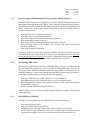
1.1
Practical Planning for Projects Using Field XRF
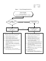
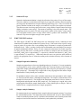
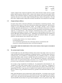
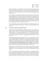
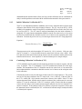
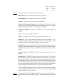
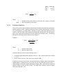
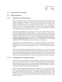
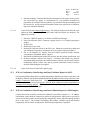
Figure 1 depicts a decision tree, which outlines the process that project planners should follow to plan
environmental projects utilizing XRF. There are three basic steps which must be followed when planning
projects that will utilize XRF analysis techniques:
1. Project scoping and determination of project DQOs
2. Ascertaining XRF needs
3. Developing the project Quality Assurance Project Plan/Sampling and Analysis Plan (QAPP/SAP)
Performing these three steps prior to sample collection will enable the project planner to ensure that the XRF
analyses are correctly executed on site and that the resultant XRF data are suitable for their intended use in site
decision making.
SOP #: X-MET 920
Rev. #:
0.0
Date:
10/29/96
Page:
6 of 39
Figure 1
Project Planning Decision Tree
Project Scoping
Review Site History
Determine Data Quality Objectives (DQOs)
Will
portable XRF analyses
achieve DQOs?
Perform full protocol
EPA methods
No
No
Yes
Will
Semi-Quantitative Screening
achieve DQOs?
Will
Quantitative Analysis
achieve DQOs?
No
Yes
Yes
SEMI-QUANTITATIVE SOP PROCESS
1)
2)
3)
4)
5)
6)
7)
Identify elements and areas of interest.
Prioritize elements of interest.
Establish possible interfering elements.
Create or modify calibration method.
Calibrate X-MET 920 with semi-quant stds.
Optimize calibration method for linearity.
Prep samples and provide splits for possible
confirmatory analysis.
8) Analyze all field samples, including blanks
and QC samples, within a valid calibration
sequence.
9) Submit confirmatory samples for lab analysis
by full protocol EPA Methods.
10) Validate results.
11) Assemble data package.
12) Write final report - Assess confirmatory
data comparability and achievement of DQOs.
QUANTITATIVE SOP PROCESS
1)
2)
3)
4)
5)
6)
7)
8)
9)
10)
11)
12)
13)
14)
Identify elements and areas of interest.
Prioritize elements of interest.
Establish possible interfering elements.
Collect SSCS spanning conc. ranges.
Provide SSCS for fixed lab analysis by
full protocol EPA Methods.
Create X-MET 920 calibration method.
Calibrate using fixed laboratory SSCS results.
Optimize calibration method for linearity.
Prep samples and provide splits for possible
confirmatory analysis.
Analyze all field samples, including blanks
and QC samples, within a valid calibration
sequence.
Submit confirmatory samples for lab analysis
by full protocol EPA Methods.
Validate results.
Assemble data package.
Write final report - Assess confirmatory
data comparability and achievement of DQOs.
SOP #: X-MET 920
Rev. #:
0.0
Date:
10/29/96
Page:
7 of 39
1.1.1
Project Scoping and Determination of Project Data Quality Objectives
Before Field XRF analysis can be integrated into a project's sampling and analysis scheme, the
project planner must establish the project DQOs. Prior to DQO development, the project planner
should obtain and evaluate as much historical information as possible about the site conditions and
history, including the results of any previous investigations at the site, so that the following
questions can be answered:
C
C
C
C
C
C
C
What and where is the contamination on the site?
What is the source of contamination on the site?
What is the purpose of sampling and analysis (data collection)?
What are the target elements of interest?
What are the Action Level concentrations for the elements of interest?
What non-target metals or site conditions may be present that could create possible
interference problems?
What is the intended use of the data?
If the project planner can answer these questions completely, then the project DQOs have been
developed properly and are understood. For assistance, refer to the Agency document Guidance
for the Data Quality Objective Process, EPA QA/G-4, which describes the informational needs
and critical decision processes that must be addressed during DQO development.
1.1.2
Ascertaining XRF Needs
Once the project target elements, action levels, and intended data uses have been established during
DQO development, the project planner can proceed with ascertaining XRF needs for the project.
The project planner should first determine whether the project DQOs can theoretically be met
using XRF techniques. If the project planner decides that XRF techniques may be applicable to
project DQOs, then the planner must answer the following questions:
C
C
C
C
What type of XRF data are required: quantitative or semi-quantitative?
What detection levels and/or action levels must be met for each target element?
What full protocol EPA methods will be used for confirmatory and/or site-specific calibration
standard (SSCS) analyses?
Will the resultant XRF data meet project objectives?
Section 2.0 discusses the basic principles of XRF analysis so that project planners will be familiar
with the technology.
1.1.3
Developing the QAPP/SAP
The XRF project planner must develop a QAPP/SAP that details the following:
C
C
C
C
Project description and DQOs,
Project personnel and their responsibilities,
Sampling protocols; sampling locations and numbers of samples to be collected,
Quality Assurance (QA) and Quality Control (QC) elements required, including frequency
requirements, acceptance criteria, and corrective actions (refer to Sections 8 and 10),
SOP #: X-MET 920
Rev. #:
0.0
Date:
10/29/96
Page:
8 of 39
C
C
C
C
SSCS analytical protocols for quantitative analysis, including frequency requirements, QC
acceptance criteria, and corrective action measures,
Confirmational analytical protocols with frequency requirements, QC acceptance criteria, and
corrective action measures (note, these protocols should be the same as the SSCS protocols
when quantitative analysis is performed),
Split sampling comparability acceptance criteria, and
How the QC and field sample data will be used to determine whether project DQOs have been
met (Data Quality Assessment).
The QAPP/SAP should reflect the complexity of the XRF project. It must sufficiently address all
of the relevant elements detailed in the Region I, EPA New England Quality Assurance Project
Plan Guidance, Draft October 1996.
Detailed standard operating procedures (SOPs) for the sampling and analysis protocols can be
referenced in the QAPP/SAP as long as the applicable SOPs are appended to that QAPP/SAP.
All SOPs that are pertinent to project operations should be developed in accordance with EPA
QA/G-6, Guidance for the Preparation of Standard Operating Procedures for Quality-related
Operations.
The QAPP/SAP must describe or reference documentation requirements for the resultant XRF and
split sample confirmation data. Documentation that all key QC elements were performed and met
project requirements is essential, regardless of intended data use. For XRF techniques, the
preparation and analysis of each batch of samples, including related standards, QC samples and
blanks, should be recorded in a field or laboratory notebook, run logs, and/or tabulated forms.
Section 13.0 of this SOP offers a detailed reporting format for XRF projects. For conventional
full protocol analytical methods, complete data packages should be produced in accordance with
the Region I, EPA-NE specifications contained in the Training Manual for Reviewing Laboratory
Data Package Completeness, dated June 1994.
Used properly, with the appropriate QC procedures and a definitive QA program, XRF can be a
very effective tool. Used without regard to QC requirements and QA process controls, the
resultant XRF data may be unusable or may not be able to be interpreted.
2.0
Method Summary
2.1
Principles of Operation
XRF is a nondestructive qualitative and quantitative analytical technique used to determine the
chemical composition of a sample. In an XRF analysis, primary X-rays emitted from an X-ray tube
or a sealed radioisotope source are utilized to irradiate a sample. The primary X-rays incident on the
sample cause the elements present in the sample to emit (that is, fluoresce) their characteristic X-ray
line spectra. The elements may be identified by the energies of the wavelengths of their spectral lines.
The unit of energy of an X-ray is the kilo electron volt (keV). The X-ray energy is proportional to the
frequency of the X-ray waves and is inversely proportional to the wavelength. Since it is a fluorescent
process, the energy of the fluorescent X-rays will always be of lower energy than the primary X-ray
energy. In addition to the fluorescent X-rays, there will be a backscattering of the primary X-rays.
Energies of the fluorescent and scattered X-rays are converted (within the detector) into a train of
electric pulses, the amplitudes of which are linearly proportional to the energy. An electronic
SOP #: X-MET 920
Rev. #:
0.0
Date:
10/29/96
Page:
9 of 39
multichannel analyzer measures the pulse amplitudes which is the basis of qualitative X-ray analysis.
The number of counts at a given energy per unit of time is representative of the element concentration
in a sample and is the basis for quantitative analysis.
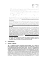
2.1.1
Fluorescent X-rays
During interaction of the primary source X-rays with samples, they may either undergo scattering
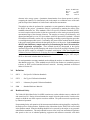
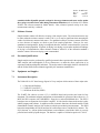
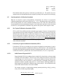
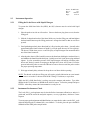
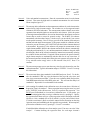
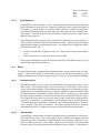
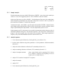
or absorption by sample atoms in a process known as the photoelectric effect. This latter
analytical phenomenon, illustrated in Figure 2, occurs when incident radiation knocks an electron
from the inner most shells of an atom. The atom, now in an excited state, releases its surplus
energy almost instantly by filling the vacancy created with an electron from one of the outer energy
shells. This rearrangement of electrons is associated with the emission of an X-ray with a
wavelength characteristic (in terms of energy) of the given atom.
Figure 2
Electron rearrangement in an atom exposed to Xray radiation generating a characteristic fluorescent
X-ray.
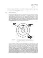
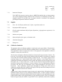
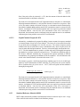
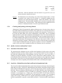
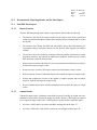
X-rays are created in the inner most shells of an atom, the K, L, and M atomic shells. Each
characteristic X-ray line is defined with the letter K, L, or M, which signifies which shell had the
original vacancy and by a subscript alpha (") or beta ($), which indicates the higher shell from
which an electron fell to fill the vacancy and produce the X-ray. For example, a K" line is
produced by a vacancy in the K shell filled by an L shell electron, whereas a K$ line is produced
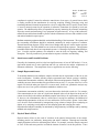
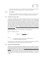
by a vacancy in the K shell filled by an M shell electron. Figure 3 is a schematic which illustrates
of the production of K and L X-rays. Since the electrons producing the fluorescent X-rays are
not valence (outer) shell electrons, the X-ray energy is not affected by the chemical or physical
form of the atom. Thus, elemental sulfur and CaSO4 give the same sulfur X-ray. Since there are
few allowed transitions, and thus relatively few X-ray lines, the X-rays for a specific element are
SOP #: X-MET 920
Rev. #:
0.0
Date:
10/29/96
Page:
10 of 39
Figure 3
Production of K and L X-rays
well defined. K lines have the shortest wavelengths and, therefore, the highest energies. L lines
have longer wavelengths and thus lower energies and M lines have very long wavelengths and thus
even lower energies.
An X-ray source can excite characteristic X-rays from an element only if the source energy is
greater than a threshold energy associated with a particular line group (K, L, or M). This energy
threshold, called the absorption edge (i.e., K absorption edge, L absorption edge, or M absorption
edge) is greater than the corresponding line energy. (Actually, the K absorption edge energy is
approximately equal to the sum of the K, L and M line energies. The L absorption
edge energy is approximately equal to the sum of the L and M line energies.) Also, the closer the
absorption edge energy of an element is to the source energy (but not greater than the source
energy), the more efficient is the excitation and the more sensitive is the element’s detection. For
example, if a source energy is sufficient enough to excite the K lines for both Zn (atomic number
30) and Ni (atomic number 28), then the Zn K lines will be more sensitive than the Ni K lines (i.e.,
the higher the atomic number, the higher the line energies, and the closer the line energy is to the
source energy). If the source energy is sufficient to excite the K lines, then they will always be
accompanied by the L and M lines of the same element. If there is insufficient energy to excite
the K lines, but enough to excite the L line, then just the L and M lines will appear. XRF
analyzers most commonly measure X-ray lines originating from the K and L shells; only elements
with an atomic number greater than 57 have measurable M shell emissions.
SOP #: X-MET 920
Rev. #:
0.0
Date:
10/29/96
Page:
11 of 39
SOP #: X-MET 920
Rev. #:
0.0
Date:
10/29/96
Page:
12 of 39
2.1.2
Scattered X-rays
Scattered or backscattered radiation is simply the reflection of the primary X-rays off the sample.
The source radiation is scattered from the sample by two physical reactions: coherent scattering
(no energy loss) and incoherent or Compton scattering (small energy loss). Thus, for each line of
primary radiation incident on the sample, two scattered X-ray lines close together are returned.
The coherent scatter lines being equal to the source energy and the Compton scatter lines being
slightly less than the source energy. The amount of scattering is due to the sample matrix. The
two primary factors are particle size and average atomic number of the sample. Larger particle
sizes and lighter matrices (lower average atomic number), produce more backscatter. The
scattered X-rays have the highest energies in the spectrum.
2.2
X-MET 920 XRF Analyzer
The EPA Region I X-MET 920 XRF analyzer has two radioisotope sources, Cadmium-109 and
Americium-241, available for the production of primary X-rays. Each source emits a specific energy
range of primary X-rays that cause a corresponding range of elements in a sample to produce their
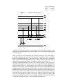
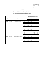
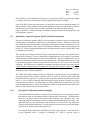
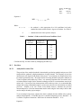
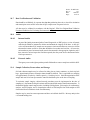
fluorescent X-rays. Table 1 provides a listing of the recommended source and analysis line energies
for typical environmental elements. The K" or L" line is always the most intense line in their respective
line group and, for that reason, is usually the line of choice for analysis (note, the intensity ratio
between K" and K$ lines is approximately 7:1, respectively, while the ratio between L" and L$ lines
is approximately 3:2, respectively). When more than one source can excite the same element of
interest, the appropriate source is selected according to the excitation efficiency of the elements of
interest.
2.2.1
Sample Preparation Summary
Samples are prepared in one of two ways depending on the type of analysis. For semi-quantitative
screening analysis, sticks, stones, and other matter that is non-representative of the sample are
removed, the sample is then thoroughly homogenized, and an aliquot is placed directly in a plastic
XRF sample cup. The sample cup is capped with a clear polypropylene film and the sample
identification is clearly labeled prior to analysis.
For quantitative analysis, sticks, stones, and other matter that is non-representative of the sample
are removed, and the sample is thoroughly homogenized. The sample is dried and then sieved
through a No. 60 mesh sieve. The fraction of the sample that passes the No. 60 sieve is then rehomogenized and aliquoted into the XRF sample cup. The sample cup is capped with a clear
polypropylene film and the sample identification is clearly labeled prior to analysis. Refer to
section 12.0 for a complete discussion of sample preparation.
2.2.2
Sample Analysis Summary
For measurement, the cup is positioned in the sample holder and exposed to primary X-rays from
the selected radiation source. The sample fluorescent and backscatter X-rays are detected and the
results are recorded by the data system. Qualitative determinations of the elements present in the
sample are based on the locations of characteristic peaks produced by individual
SOP #: X-MET 920
Rev. #:
0.0
Date:
10/29/96
Page:
13 of 39
Table 1
Recommended Source and X-ray Line Selection
for Typical Elements of Environmental Concern
Recommended Analysis Lines
Isotope
Cd-109
Am-241
Half Life
1.3 Years
433 Years
Primary Radiation
Ag K X-ray, 22.1 keV
Gamma Radiation, 59 keV
Element
K Line (keV)
K"
K$
Cr
5.41
5.95
Mn
5.89
6.49
Fe
6.40
7.06
Co
6.92
7.65
Ni
7.47
8.30
Cu
8.04
8.94
Zn
8.63
9.61
As
10.5
11.8
L Lines (keV)
L"
L$
Hg
9.98
11.9
Tl
10.3
12.3
Pb
10.5
12.6
Mo
17.4
19.8
Ag
22.1
25.2
Cd
23.1
26.4
Sn
25.2
28.8
Sb
26.2
30.1
Ba
32.0
36.8
SOP #: X-MET 920
Rev. #:
0.0
Date:
10/29/96
Page:
14 of 39
elements in the energy spectra. Quantitative determination of an element present is made by
comparing the intensity of a characteristic peak in the sample to a calibration curve of the same
peak developed from standards of similar matrix and known concentrations.
The analysis can either be performed in a quantitative or semi-quantitative fashion depending on
the DQOs of the project. Quantitative analysis is performed by matching the matrix of the
standards to that of the site. These standards, called “site specific calibration standards (SSCS)”
are actual samples taken from the site that are representative of the matrix present and span the
concentration range of the elements of interest. The samples are sent to a fixed laboratory, acid
digested, and analyzed by AA or ICP in accordance with a full protocol EPA methods. It should
be noted that confirmatory results will vary depending on whether a partial digestion procedure
or a total digestion procedure is used. Confirmatory full protocol EPA methods should be chosen
in the project scoping phase and meet the data quality objectives of the project. It is essential that
all SSCS and confirmatory sample analyses be performed using the same EPA methods for
sample preparation and analysis. These methods should be documented in the Quality
Assurance Project Plan (QAPP)/Sampling and Analysis Plan (SAP) and DQO Summary Form.
Once the SSCS results are validated in accordance with Region I, EPA New England Data
Validation Functional Guidelines for Evaluating Environmental Analyses and deemed usable, they
are considered the true values of the SSCS and can be used in calibrating the XRF analyzer.
SSCS are discussed in further detail in Section 8.1.
For semi-quantitative screening, standards used to calibrate the analyzer are obtained from sources
other than the project site. These standards may be SSCS from another site, standards prepared
in-house, or NIST certified standard reference materials. Screening standards are discussed
further in Section 8.2.
3.0
Definitions
3.1
SSCS -
Site Specific Calibration Standards
3.2
STCS -
Site Typical Calibration Standards
3.3
LPCS -
Laboratory Prepared Calibration Standards
3.4
SRM
Standard Reference Material
4.0
Health and Safety
-
The X-Met 920 Solid State Probe Set (SSPS) contains two nuclear radiation sources; cadmium 109
and Americium 241. During all measurements the sample lid on the probe must be closed over the
sample to shield the user from exposure to nuclear radiation. The probe must not be opened except
by authorized personnel.
Proper training for the safe operation of the instrument and radiation training should be completed by
the analyst prior to field operations. Radiation safety information for the X-MET 920 can be found
in the operators manual. Protective shielding should never be removed by the analyst or any personnel
other than the manufacturer. The analyst should be aware of the local, state and national regulations
that pertain to the use of radiation-producing equipment and radioactive materials with which
SOP #: X-MET 920
Rev. #:
0.0
Date:
10/29/96
Page:
15 of 39
compliance is required. Licenses for radioactive materials are of two types; (1) general license which
is usually provided by the manufacturer for receiving, acquiring, owning, possessing, using, and
transferring radioactive material incorporated in a device or equipment, and (2) specific license which
is issued to named persons for the operation of radioactive instruments as required by local state
agencies. The radiation safety officer is responsible for properly instructing all personnel, maintaining
inspection records and monitoring X-ray equipment at regular intervals. A copy of the radioactive
material license and leak tests should be present with the instrument at all times and available to local
and national authorities upon request.
Radiation monitoring equipment should be used with the handling of the instrument. The operator and
the surrounding environment should be monitored continually for analyst exposure to radiation.
Thermal luminescent detectors (TLD) in the form of badges and rings are used to monitor operator
radiation exposure. The TLDs should be worn in the area of most frequent exposure. The maximum
permissible whole-body dose from occupational exposure is 5 Roentgen Equivalent Man (REM) per
year. Possible exposure pathways for radiation to enter the body are ingestion, inhaling, and
absorption. The best precaution to prevent radiation exposure is distance and shielding.
5.0
Interferences and Potential Problems
Generally, the instrument precision is the least significant source of error in XRF analysis. User or
application related error is more significant and will vary with each site and the completeness of
instrument calibration. The components of user or application error are the following:
5.1
Sample Representativeness
To accurately characterize site conditions, samples collected must be representative of the site or area
under investigation. Variables affecting sample representativeness include: geologic variability,
contaminant concentration variability, and sample collection and preparation variability. Geologic
variability can occur when more than one type of matrix exists on site (i.e., one part of the site is a rich
organic soil while the other part of the site is a course sand). In this case, quantitative analysis may
require two sets of site-specific calibration standards to minimize error.
Contaminant concentration variability is an issue that must be dealt with at each site. For example,
if the contamination on site is due to a liquid waste dumped in the soil, the dispersion in the area of
concern is more likely to be uniform, and thus the samples more likely to be representative of the area.
If, however, the contamination is due to a solid waste of varying size and shape, the likelihood of
samples being representative of the area is lower and thus the error in results is greater. In this latter
case, the error can be minimized by homogenizing a large volume of sample prior to analyzing an
aliquot, or by analyzing several samples at each sampling point and averaging the results.
Preparation and analytical variability are minimized by using consistency in technique and by matching
standard and sample matrices.
5.2
Physical Matrix Effects
Physical matrix effects are the result of variations in the physical characteristics of the sample,
including particle size, uniformity, homogeneity and surface condition. Thorough and consistent
sample preparation is critical to minimizing these effects. For example, consider a sample composed
of a mix of fine and coarse particles in which the element of interest is in the fine particles. If two
SOP #: X-MET 920
Rev. #:
0.0
Date:
10/29/96
Page:
16 of 39
separate aliquots of the sample are prepared in such a manner that one sample receives a greater
portion of the fine particles, then the relative volume of the element of interest in each sample will be
different. Thus, when these samples are analyzed, a larger amount of the element of interest will be
exposed to the source X-rays in the sample containing the larger volume of fine particles. This will
then result in a higher intensity reading and a measured concentration in the sample that is biased high.
5.3
Chemical Matrix Effects
Chemical matrix effects result from differences in concentrations of interfering elements. These
interelement effects appear as either X-ray absorption or enhancement phenomena. Both effects are
common in soils contaminated with heavy metals. For example, consider a series of samples
containing nickel (Ni) and chromium (Cr). Ni in the sample will absorb the fluorescent X-ray of Cr.
If the concentration of Cr remained constant and the Ni concentration increased, then the detected
signal for Cr would decrease. Thus, basing the concentration solely on the Cr signal, the Cr
concentration would appear to decrease. In order to correct for this absorption effect on Cr, a term
must be added to the regression equation for Ni. (Information on developing regression equations for
instrument calibration is discussed at length in the X-MET 920 reference manual.) As a general
guideline, elements that may cause chemical matrix effects are:
1) near the target element (± 4 or 5 atomic numbers),
2) excited by the source,
3) at a concentration greater than 10% of the target element’s concentration, and
4) present in varying concentrations in the area under investigation.
It is essential to define the chemical matrix effects on the elements of interest prior to instrument
calibration.
5.4
X-ray Spectrum Overlap
Certain emitted X-ray lines from different elements, when present in the sample, can be very close in
energy and, therefore, interfere by producing an overlapping spectrum. Typical spectrum overlaps are
caused by the K$ line of element Z-1 overlapping the K" line of element Z, where Z = the atomic
number of the element. (Note, in heavier elements, the K$ line of elements Z-2 or Z-3 may create the
spectral overlap of the K" line of element Z.) This is called the K"/K$ interference. Since the K":K$
intensity ratio for a given element usually varies from 5:1 to 7:1, the interfering element must be
present at a large concentration to disturb the measurement of element Z.
For example, a large concentration of vanadium (Z = 23) could interfere with chromium (Z = 24).
Vanadium (V) has K" and K$ energies equal to 4.951 and 5.427 keV, respectively. Chromium (Cr)
has a K" energy equal to 5.41 keV. Since the resolution of the Si(Li) detector in the X-MET 920 is
approximately 0.170 keV, large amounts of vanadium in the sample will result in spectral overlap of
the V K$ with the Cr K" peak and the measured X-ray spectrum will include total counts for Cr plus
V lines.
Other spectral interferences can occur between K/L, K/M, and L/M lines. An example is the As K"/Pb
L" interference. In this case the lead can be measured from the Pb L$ line, and arsenic from either the
As K" or As K$ line; in this way the interference can be overcome. The X-MET 920 uses correction
factors obtained from the analysis of single element standards to correct for spectrum overlap. It is
SOP #: X-MET 920
Rev. #:
0.0
Date:
10/29/96
Page:
17 of 39
essential to define all possible spectral overlaps for the target elements and create and/or update
the overlap correction factor table during instrument calibration (refer to Section 9.2.3 and the
X-MET 920 reference manual for further details). Note, whenever spectral overlap is an issue,
measurement sensitivity is reduced.
5.5
Moisture Content
Sample moisture content will affect the accuracy of the sample results. The measurement error may
be minor when the moisture content is small (5-20 %), or it may be significant when measuring the
surface of soils that are saturated with water. For quantitative analysis, moisture content will not be
an issue because all samples are dried as part of the sample preparation. However, for semiquantitative screening analysis, drying is not required, therefore, moisture content should be a practical
concern in sample preparation. In general, air drying, oven drying, or some other mechanical technique
of drying is recommended to reduce moisture content to within 5% of the calibration standard’s
moisture content. Microwave drying is not recommended.
6.0
Personnel Qualifications
Sample analysis must be performed by qualified personnel either experienced in the operation of the
XRF analyzer and knowledgeable in X-ray fluorescence, or under the direct supervision of an
experienced and knowledgeable individual. The analyst must be thoroughly familiar with this SOP
and the X-Met 920 Reference Manual supplied by the instrument manufacturer.
7.0
Equipment and Supplies
7.1
Instrument Description
The X-Met 920 is a PC based energy dispersive X-ray analyzer which consists of three major units:
1.) Computer and Software
2.) X-Met PC Unit (XPCU)
3.) Solid State Probe Set (SSPS).
The X-MET 920 software (version 1.33), is MS-DOS based and provides total control of the
instrument. The minimum computer configuration recommended for operation of the software is a 33
MHZ 486 DX computer with 2 MB RAM, 1 floppy drive, and an 80 MB hard drive. The XPCU
board goes into an expansion slot inside the computer. It is the interface between the analysis probe
and the computer and software. In addition to other electronic functions, this board contains a 2048
channel Multi Channel Analyzer (MCA) that records the spectra during measurements. The SSPS
houses the sample holder, the Cd-109 and Am-241 radioisotope sources, and the Si(Li) detector. The
Si(Li) detector is a silicon (drifted with lithium) semi-conductor crystal diode which is reversely
polarized and cooled by liquid nitrogen. The detector is capable of resolution equal to 0.170 keV.
SOP #: X-MET 920
Rev. #:
0.0
Date:
10/29/96
Page:
18 of 39
7.1.1
Instrument Transport
The X-MET 920 (computer, monitor, probe etc.) MUST be handled with care during transport.
The original shipping containers should be used at all times to avoid damage in transit. The
shipping container for the SSPS must be properly labeled in accordance with regulations
governing the shipment of radioactive materials.
7.2
Supplies
7.2.1
Sieve: No. 60 (250 µm) stainless steel, Nylon, or equivalent mesh sieve
7.2.2
Polyethylene XRF sample cups
7.2.3
Film for sample containment: Mylar, Kapton, Spectrolene, polypropylene or equivalent; 2.5 or
6.0 µm thick
7.2.4
Stainless steel spoons
7.2.5
Mortar and pestle: glass, agate, or aluminum oxide
7.2.6
Aluminum drying pans
7.2.7
Drying oven
8.0
Calibration Standards
The appropriate choice of calibration standards is made based on the project DQOs. When definitive
quantitation is required, site-specific calibration standards must be used (refer to Section 8.1). When
semi-quantitative results are required, the choice of the appropriate semi-quantitative calibration
standards is made (refer to Section 8.2).
The first step in selecting the calibration standards is to determine the target elements of interest. The
basic rule is to prioritize the target elements and then reduce the number of elements to be analyzed
in the field to the minimum amount required to perform the task. For example, suppose the site
requiring cleanup was a metals plating facility which contained a waste lagoon known to be
contaminated with high concentration of several metals, and cadmium was the element present with
the highest risk (i.e., lowest action level). In this case, the amount of target elements required to
monitor the cleanup could be reduced to 1 element, cadmium. Here, by simplifying the calibration
procedures and using only one radioisotope source, sample throughput for the project can be
maximized. Note, confirmatory samples taken throughout the cleanup and a final round of
confirmatory sampling following completion of the project will help ensure that cleanup action levels
for all target elements of interest were obtained.
Another reason to reduce the number of target elements to be analyzed in the field applies directly to
quantitative analysis using site-specific calibration standards (SSCS). In order to properly model the
regression equation for an element, additional SSCS must be included for each element that may cause
possible chemical matrix effects (approximately five per interfering element). Thus, by reducing the
number of target elements, the number of required SSCS can be significantly reduced, the complexity
SOP #: X-MET 920
Rev. #:
0.0
Date:
10/29/96
Page:
19 of 39
of the calibration can be simplified, and a large cost savings can be realized by reducing the number
of samples that require fixed laboratory analysis using full protocol EPA methods.
Note, the X-MET 920 can only analyzed ten (10) elements at one time in a calibration method. Of
those 10 elements, only 6 elements may be reported quantitatively and of the remaining four elements,
one must always be the backscatter peak (the Compton K" peak from the source radiation).
Figure 1 (Section 1.1) illustrates the typical sampling and analysis scheme for both quantitative and
semi-quantitative analyses.
8.1
Quantitative Analysis Using Site-Specific Calibration Standards
Site-specific calibration standards (SSCS) are actual samples from the site under investigation that
span the range of concentrations found on site for the elements of interest. Elements of interest not
only include the target elements under investigation, but also those elements present that may create
possible interference effects. SSCS must be representative of the matrix under investigation (refer to
Section 5.1). If there are distinctly different matrices on site that require analysis, separate SSCS must
be sampled for each matrix.
The concentration of all target elements, and any elements present that may cause chemical matrix
effects (refer to Section 5.3), must be determined by independent AA or ICP analysis in accordance
with the full protocol EPA methods specified in the QAPP/SAP. (The same method must be used to
perform all confirmatory analyses to ensure data comparability.) Independent SSCS analyses must
be performed in triplicate and the average result for each element is to be used in the instrument
calibration. SSCS data must be validated in accordance with the most recent version of the Region
I, EPA-NE Data Validation Functional Guidelines for Evaluating Environmental Analyses prior to use
and all raw data and information must be provided with the data package to ensure the scientific
defensibility of the calibration standards.
The X-MET 920 reference manual uses the term “modeling” to describe the process of modifying the
regression equation of an element’s calibration curve to correct for chemical matrix effects and
backscatter from the X-ray source. To properly model a regression equation and compensate for these
effects, a series of SSCS, containing both interfering and target elements at known and varying
concentrations, are required. The total number of SSCS required increases significantly with each
target and interfering element. (Again, by reducing the number of target elements in the analysis, the
number of SSCS required may be greatly reduced.)
8.1.1
Site-Specific Calibration Standard Sampling
Collect sufficient SSCS to generate a minimum 5-point calibration curve for each target element,
that spans the range of concentrations found in the area under investigation. The high and low
SSCS for each target element will determine that element’s linear calibration range. The
remaining standard concentrations should be roughly distributed throughout this range. Note,
additional SSCS near the concentration range of interest or site action level will improve the
accuracy of the calibration at that level. For each interfering element present, increase the number
of SSCS for the element being interfered with, by 5.
For example, consider an analysis in which Pb and Cr are the target elements. To develop the two
5-point calibration curves, it required a combination of 7 SSCS to span the range of
SOP #: X-MET 920
Rev. #:
0.0
Date:
10/29/96
Page:
20 of 39
concentrations found on site. Unfortunately, Ni was also present in high enough concentrations
to cause a chemical matrix effect with the Cr X-ray. In order to improve the calibration model and
reduce the chemical matrix effects, 5 more Cr SSCS which contain Ni, are added to the Cr
calibration curve. Thus, a total of 12 SSCS are now needed to calibrate the instrument for the
two target elements.
SSCS collected for an interfering element should reflect the variability of that element’s
concentration found in relation to the concentration of the target element. (Note, mixing of high
and low concentration soils to provide a full range of target element concentrations is not
recommended because the ratio of the interfering element to the target element will remain the
same and the interelement effect in the calibration will be skewed in one direction.) All target and
interfering element concentrations, in each of the SSCS collected, should be included as calibration
points. Outliers can later be eliminated when the regression equations are being developed (refer
to “developing regression equations” in the reference manual).
To assist in determining appropriate SSCS for laboratory analysis, sample points may be prescreened with the instrument calibrated using semi-quantitative calibration standards (refer to
Section 8.2).
8.1.2
Site-Specific Calibration Standard Preparation
The SSCS samples collected in the field must be oven-dried at < 150EC for 2 to 4 hours to remove
moisture. The entire sample should be spread out in a drying pan and clumps broken up with a
stainless steel spoon. If mercury is to be analyzed, a separate sample must be air dried until the
moisture content is < 20 %, as heating may volatilize the mercury. After drying, all large organic
debris and non-representative material (sticks, twigs, leaves, roots, insects, asphalt, rocks, etc.)
are removed and the sample is transferred to a mortar and ground with a pestle to a uniform
consistency.
The dried and ground sample is then sieved through a No. 60 (250 µm) mesh stainless steel sieve.
At no time should the material be forced through the sieve. Pebbles and organic matter remaining
on the sieve should be discarded. The under-sieve fraction of the material constitutes the sample.
(Although a maximum final particle size of 60-mesh is normally recommended, a smaller sieve
size may be used if the physical characteristics of the sample or DQOs of the project dictate.
Note, the identical sieve size must be used to prepare all SSCS and samples. Deviations in the
sieve size and the reason for the change should be documented in an amendment to the QAPP/SAP
and must be recorded in the sample preparation log and noted in the final report.)
Homogenize the sieved sample by placing 150 - 200 grams of sample on a piece of kraft or
butcher paper about 1.5 by 1.5 feet in size. Each corner of the paper should be lifted alternately,
rolling the soil over on itself and toward the opposite corner. The soil should be rolled on itself
20 times.
Fill one or more XRF sample cups approximately 3/4 full with sample. Cut and tension (wrinklefree) a piece of polypropylene film over the top of the cup and seal using the plastic film securing
ring. Label the sample cups appropriately. The remainder of the sample is then split into two
portions and placed in clean labeled glass or plastic containers. One portion of the sample is
submitted to the approved laboratory for analysis of the requested element(s) by the full protocol
SOP #: X-MET 920
Rev. #:
0.0
Date:
10/29/96
Page:
21 of 39
EPA methods, and the other portion is archived for possible future use. The stainless steel sieve
and spoons must be decontaminated between samples by washing with soap and water and drying.
8.2
Semi-Quantitative Calibration Standards
When the site objectives require semi-quantitative measurements, the choice of an appropriate
calibration standard must be determined (Sections 8.2.1 - 8.2.3). Depending on the relative accuracy
of the screening desired, one or more calibration standards may be used. Note, due to the differences
in representativeness between standards and samples, as well as the other interference factors described
in Section 5.0, semi-quantitative calibrations may generate false positive and/or negative results.
8.2.1
Site Typical Calibration Standards (STCS)
STCS are SSCS from a different site that contain the target elements of interest in the approximate
range and matrix as the site under investigation. If possible, STCS should be chosen to reflect any
chemical matrix effects that may be present in the samples on site. A new instrument calibration
must be performed in accordance with Section 9.1 each time STCS are employed. STCS data
must be validated in accordance with the most recent version of the Region I, EPA-NE Data
Validation Functional Guidelines for Evaluating Environmental Analyses prior to use and all raw
data and information must be provided with the data package to ensure the scientific defensibility
of the calibration standards.
8.2.2
Laboratory Prepared Calibration Standards (LPCS)
If satisfactory STCS are not available for all elements at appropriate concentrations, it may be
necessary to prepare quantitative standards from laboratory stock chemicals. Such standards may
be prepared by mixing finely ground dry chemicals or liquid standards with a clean soil, silica sand
or other inert material (e.g. Somar Mix, from Somar Laboratories, NY, NY, or equivalent).
8.2.2.1
Solid Chemical Prepared LPCS
Prepare the high LPCS first, by adding a known weight of dry chemical(s) to a known weight
of clean dry soil or inert material. The clean soil or inert material must first be pre-dried and
sieved through a No. 60 (250 µm) sieve. Following the addition of the dry chemical, the
combined mixture must be ground in a mortar and pestle to thoroughly homogenize the
standard to a uniform consistency and particle size. Serial dilutions of the high standard may
then be prepared to establish the calibration range for the analysis. All serial dilutions must
mixed in the identical manner as the initial standard.
For example, to prepare a 10,000 mg/kg antimony standard, add 0.60 g of Sb2O3 to 49.4 g
of dry clean soil and mix/grind thoroughly.
(600 mg Sb2O3) (83.5 % Sb)
(0.050 kg)
' 10,000 mg/kg Sb
SOP #: X-MET 920
Rev. #:
0.0
Date:
10/29/96
Page:
22 of 39
Note, if the purity of the dry chemical is < 97%, then the amount of chemical added or final
concentration must be adjusted to reflect this.
The clean soil or inert material used in LPCS preparation must be analyzed as a control blank,
following instrument calibration, to verify that the elements of interest are not present. If the
soil or inert matrix contains an element of interest, its concentration must be determined by
the method of standard addition and the actual LPCS concentrations must be corrected for this
amount. A minimum of 3 LPCS and the unspiked matrix are required to perform the method
of standards addition. Once the base level concentration of the soil or inert matrix is
determined, the instrument must be recalibrated using the unspiked matrix as an additional
calibration point along with the corrected LPCS concentrations.
8.2.2.2
Liquid Chemical Prepared LPCS
Alternatively, a standard may be prepared by adding a known amount of an aqueous standard
to a known amount of clean soil or inert material. The clean soil or inert material must first
be pre-dried and sieved through a No. 60 (250 µm) sieve. The volume of aqueous metals
standard used must be sufficient to create a standard/soil slurry where all parts of the soil
come in contact with the liquid standard. The slurry is then thoroughly mixed and dried at #
105EC. The dried standard must be ground in a mortar and pestle to thoroughly homogenize
the standard to a uniform consistency and particle size. To establish a calibration range for
the analysis, additional standards may be prepared from aqueous standards of different
concentrations, or by preparing serial dilutions of the first standard. All serial dilutions must
mixed in the identical manner as described in Section 8.2.2.1.
For example, to prepare a 10,000 mg/kg antimony standard, pipet 10 mL of a 10,000 mg/L
antimony AA/ICP standard into a beaker containing 10 g of dry clean soil or inert material.
Mix to a uniform slurry, dry in an oven at # 105EC, and re-mix/grind until the standard is
thoroughly homogenized.
(10,000 mg/L Sb) (0.010 L)
' 10,000 mg/kg Sb
(0.010 kg)
The clean soil or inert material used in LPCS preparation must be analyzed as a control blank,
following instrument calibration, to verify that the elements of interest are not present. If the
soil or inert matrix contains an element of interest, its concentration must be determined by
the method of standard addition and the actual LPCS concentrations must be corrected for this
amount. A minimum of 3 LPCS and the unspiked matrix are required to perform the method
of standards addition. Once the base level concentration of the soil or inert matrix is
determined, the instrument must be recalibrated using the unspiked matrix as an additional
calibration point along with the corrected LPCS concentrations.
8.2.3
Standard Reference Material (SRM)
NIST or other commercially available certified standard reference materials may be used. A copy
of the certified results must be included in the final data package.
SOP #: X-MET 920
Rev. #:
0.0
Date:
10/29/96
Page:
23 of 39
SOP #: X-MET 920
Rev. #:
0.0
Date:
10/29/96
Page:
24 of 39
9.0
Calibration and Operation
9.1
Instrument Calibration
The X-MET 920 may be calibrated using one of several techniques available depending on the data
quality objectives of the project.
C
For quantitative field analysis, empirical calibration procedures must be used that incorporate sitespecific calibration standards.
C
For semi-quantitative screening, one of three calibration procedures, empirical calibration,
fundamental parameters calibration, or Compton peak normalization calibration, may be used to
calibrate the instrument depending on the standards and instrument software available.
Empirical Calibration - The standard software package supplied with the X-MET 920 supports the
empirical calibration technique. This calibration technique is used for all quantitative analyses and
for semi-quantitative analysis using a series of either site-typical calibration standards, laboratory
prepared calibration standards, or standard reference materials. Refer to Instrument Operation,
Section 9.2 of this SOP, and X-MET reference manual for information on performing an empirical
calibration.
Fundamental Parameters - Alternatively, an optional software package called ACES (Automated
Contaminant Evaluation Software), is available which uses a modified fundamental parameter
approach to generate a calibration. This calibration technique may only be used for semi-quantitative
screening analyses. This calibration relies on the ability of the liquid nitrogen cooled, Li(Si) solid state
detector to separate the coherent (Rayleigh) backscatter peaks from the incoherent (Compton)
backscatter peaks of primary radiation. These peak intensities are known to be a function of sample
composition, and the ratio of the Compton to Rayleigh peak is a function of the mass absorption of
the sample. The calibration procedure is explained in detail in the ACES user’s manual. The ACES
program is not presently available on the Region I X-MET 920, and thus, the fundamental parameters
calibration procedure is beyond the scope of this SOP and will not be addressed further.
Compton Peak Normalization - The last calibration technique, Compton peak normalization, is a
manual calibration technique used for semi-quantitative screening analyses. It is based on the analysis
of one or more certified standards, where the intensities of the lines of interest (i.e., target elements)
in the sample are ratioed against those in the standard, following normalization of the Compton peaks.
The Compton peak intensity changes with differing matrices. Generally, matrices dominated by lighter
elements produce a larger Compton peak, and those dominated by heavier elements produce a smaller
Compton peak. Normalizing to the Comptom peak is similar to using internal standard calibration and
can reduce the problems associated with varying sample matrices. Use Equation 5 to calculate
Compton peak normalized sample results.
SOP #: X-MET 920
Rev. #:
0.0
Date:
10/29/96
Page:
25 of 39
Equation 5
Sample Concentration (mg/Kg) '
(AI) (SK) (SC)
(AK) (SI)
Where:
AI
AK
SK
SI
SC
=
=
=
=
=
Baseline corrected sample intensity
Baseline corrected sample Compton K" intensity
Baseline corrected standard Compton K" intensity
Baseline corrected standard intensity
Standard concentration (mg/Kg)
Certified standards, used in Compton peak normalization calibrations, may include either SSCS,
STCS, LPCS, or SRM. For optimum results, the certified reference standards should be of similar
matrix as the samples and should contain the elements of interest at concentrations near those expected
in the samples. Although the X-MET 920 software can be adapted to supply the line intensities to
manually calculate Compton peak normalized results, it is not a routine procedure accommodated by
this instrument and will thus not be addressed further in this SOP.
9.1.1
Instrument Performance Check
Prior to the analysis of any standards or samples, the peak calibration of the X-MET 920 must
be verified. The channel for the Pb L$ line (on the multi-channel analyzer of the XPCU board)
must be verified at the beginning of the day (prior to the initial calibration) and at the end of the
analysis sequence or every 8 hours, whichever is more frequent. If the initial peak calibration
check at the beginning of the day for the Pb L$ line is not at 990 ± 2 channels, re-set the peak
calibration, verify that it is correct, and perform an initial calibration. If the peak calibration
check performed at the end of the analytical sequence (or after eight hours) does not meet the
above criteria, then re-set the peak calibration, re-perform the initial calibration and re-analyze all
samples since the last compliant peak calibration check. All samples must be analyzed within a
valid analytical sequence.
9.1.2
Initial Calibration (ICAL)
This SOP is specific to the use of empirical calibration. The other calibration techniques for semiquantitative analysis, fundamental parameters and Compton peak normalization, are acceptable
for use, but will require modifications to this SOP (Sections 9.1.2 and 9.2.3) and documentation
of these changes in the QAPP/SAP. All other procedures discussed in this SOP are valid for these
other calibration techniques and should remain implemented.
After the peak calibration check criteria are met, and prior to the analysis of any samples, the XMET 920 must be calibrated empirically for quantitative or semi-quantitative analysis. The
instrument must be calibrated at a minimum of once every seven (7) days for the Cd-109 source,
once every thirty (30) days for the Am-241 source, and any time the continuing calibration
verification criteria below are not met. The correlation coefficient of the calibration curve for each
target element must be $0.98. If the correlation coefficient is less than 0.98, the problem must be
identified and corrected prior to sample analysis. If a correlation coefficient of $ 0.98 is
SOP #: X-MET 920
Rev. #:
0.0
Date:
10/29/96
Page:
26 of 39
unattainable due the chemical matrix effects, the best possible calibration must be established for
analysis and the problems associated with the calibration documented in the report narrative.
9.1.3
Initial Calibration Verification (ICV)
The ICV is an independent standard (or standards), from a source other than that used in the initial
calibration, that contains all the target elements of interest. The ICV may be an STCS, LPCS,
or SRM, or for quantitative analysis using SSCS, an additional SSCS not used in the ICAL may
be used for the ICV. The ICV must be analyzed immediately after the initial calibration is
completed. ICV target element concentrations should be near the site action levels, or if no action
level has been determined, they should be near the level of interest or the mid-point of the initial
calibration. Calculate the percent recovery for each target element in the ICV using Equation 6.
Equation 6
Percent Recovery (%) '
Found Value
x 100
True Value
The percent recovery for each element in the ICV must be 50 - 150 %, inclusive. If the true value
of an ICV element is < 2 times the MDL, then the control limit is the true value ± MDL. If the
ICV does not meet the control limits, then the analysis must be terminated, and the problem must
identified and corrected. An acceptable ICV must be obtained prior to sample analysis.
9.1.4
Continuing Calibration Verification (CCV)
A CCV standard(s) must be analyzed at the beginning and end of an analysis sequence and after
every 10 samples. The CCV standard(s) is an ICAL standard that contains all of the target
elements. The concentration of the CCV should be near the site action level, or if no action level
has been determined, the concentration should be near the level of interest or the mid-point of the
initial calibration.
Calculate the percent recovery for each target element in the CCV using Equation 6. The percent
recovery for each target element in the CCV must be 80 - 120 %, inclusive. If the true value of
the CCV is $MDL and < PQL, then the control limit is the true value ±MDL. If the CCV does
not meet the control limits, then the analysis must be terminated, the problem must be corrected,
and the CCV must be reanalyzed. If the CCV reanalysis yields a result within the acceptance
criteria, then the analysis may continue and all samples analyzed since the last compliant CCV
must be re-analyzed. If the reanalysis of the CCV still does not meet the acceptance criteria, than
the instrument must be recalibrated, the ICV verified and all affected samples reanalyzed within
a valid analytical sequence.
SOP #: X-MET 920
Rev. #:
0.0
Date:
10/29/96
Page:
27 of 39
9.2
9.2.1
Instrument Operation
Filling the Probe Dewar with Liquid Nitrogen
To operate the Solid State Probe Set (SSPS), the Si(Li) detector must be cooled with liquid
nitrogen.
1. Place the probe on its side on a flat surface. Unscrew the dewar plug (brass screw) from the
filling port.
2. Slide the L-shaped outlet tube of the funnel all the way into the filling port and hand tighten
the brass knurled nut on top the filling port thread. Arrange the funnel so that its cone faces
upward.
3. Pour liquid nitrogen slowly into a funnel and let it flow into the probe dewar. It usually takes
approximately three funnel volumes of liquid N2 to fill the probe dewar (0.45 liter capacity).
The dewar is filled when you see a cone-like spray of liquid nitrogen from around the brass
nut of the funnel connector.
4. After the probe dewar is filled, carefully unscrew the funnel nut (holding the insulated sleeve)
and withdraw the funnel from the dewar port. Quickly screw back in the dewar plug and hand
tighten. In a few seconds the pressure of the liquid nitrogen will build up inside the probe
dewar and "hissing" sounds of escaping gas through relief valves will be heard. Press the
green switch on the probe to secure the radioactive sources from use until the probe reaches
the proper operating temperature.
5. Wait approximately thirty minutes for the probe to cool down before operating.
NOTE: The threads on the dewar filling port will require periodic lubrication on a semi-annual
basis or as needed. Lubricate with DOW Corning 33 Lubricant, or equivalent.
While the Si(Li) Solid State Probe is cooling, turn on the computer and monitor. Type either
SSPSA for the Cd-109 Source, or SSPSB for the AM-241 source. Follow the prompts and press
ENTER. After thirty minutes the instrumentation is ready for use.
9.2.2
Instrument Performance Check
The Lead (Pb) L$ peak optimum must be checked before instrument calibration or analysis is
performed, and at the end of the analytical sequence, or every eight hours, whichever is more
frequent.
To assure proper peak assignment and identifications, you must check to make sure the Pb L$ peak
(right side large Pb peak) is at channel 990 ± two channels. To do this, place the pure element Pb
standard into the SSPS probe sample holder.
SOP #: X-MET 920
Rev. #:
0.0
Date:
10/29/96
Page:
28 of 39
The Main Menu for X-Met 920 Software (Version 1.33, November 1994) consists of:
1.) ANALYSIS
2.) CALIBRATION
3.) MAINTENANCE
From the main menu of the computer, arrow down to MAINTENANCE and press ENTER.
Press F3 for Instrument
Press F3 for Test Measurement
Press F3 for Time
When in Time, type 30 (for 30 second analysis time) and press "ENTER".
The screen message says "Probe in Reference position. Press Start to begin"
On the base of the SSPS probe, push the red start button, and then Press F1 on the keyboard to
start acquisition. When acquisition is complete, check to see that Pb L$ peak is at channel 990 ±
two channels. To do this, move the yellow cursor to the Pb L$ peak (second large peak on screen
which is shaded) and read the channel number where the area count is at the maximum. If the Pb
L$ peak is at 990 + two channels, press F8 to quit. If not, press F8 again and type the letter “O”
to optimize. After optimization, repeat the above procedure to make sure the Pb L$ peak
assignment is proper.
The Instrument is now ready for use. In order to perform sample analysis using empirical
calibration, a new calibration method must be developed or an existing calibration method must
be updated.
9.2.3
Empirical Calibration and Method Development
Refer to the reference manual for more complete information on software operation. Particular
attention must be given to the calibration sections in the manual describing the setting of regression
terms to establish the best possible instrument calibration for analyzing field samples.
NOTE: Since sources decay, net count rates for elements will vary as time passes.
Therefore, calibration standards must be analyzed and the calibration updated at a minimum
of once every seven (7) days for the Cd-109 source and once every thirty (30) days for the
Am-241 source. Calibration records must be maintained during an ongoing project to insure that
the X-MET 920 is calibrated at the proper frequency.
To perform an empirical calibration for either quantitative analysis or semi-quantitative screening,
follow the steps below:
Screen 1:
To begin a new calibration, follow the prompts:
1. At the Main Menu arrow down to CALIBRATION and press “ENTER”
2. Press “F1" for New Method
SOP #: X-MET 920
Rev. #:
0.0
Date:
10/29/96
Page:
29 of 39
Screen 2:
Answer the questions at the prompt which are as follows:
Method Name: (Up to 8 alphanumeric characters) "ENTER"
Calibration Date: (Computer fills this in for you) “ENTER”
Operator: (Type the two initials of your name) “ENTER”
Number of Measurement Windows: (Type the number of elements you will be
analyzing for in this method and ADD one for the backscatter peak. For example,
if you were analyzing Pb and Cr, you would type 3) "ENTER"
Number of Standards: (Number of standards to be used in the calibration)
"ENTER"
Probe: (Arrow down to SSPS) "ENTER"
Window 1: (Computer automatically puts in BS [Backscatter] for you)
Window 2: (Type in one element symbol for an analyte of interest, i.e., Pb).
"ENTER" Continue entering the remaining elements of interest, both target elements
and matrix elements, in the additional window slots (up to 10 total).
Window Time: 60 (Leave at 60) "ENTER" This is the default analysis time used
to measure single element standards for setting each element’s measurement window.
From this information the software automatically calculates the overlap correction
factors.
Standard Time: 120 "ENTER" The default time for standard analysis is 120
seconds.
Analysis Time: 120 "ENTER" The default time for sample analysis is 120 seconds.
This time may be altered depending on the DQOs of the project. Analysis times
generally range from 60 - 300 seconds. Longer count times improve the precision
or reproducibility of the measurement, however increasing the count time by a factor
of 4 will provide only 2 times better precision, so there is a point of diminishing
returns. Increasing the count time also decreases the detection limit, and decreases
sample throughput. Standard and sample analysis times should be identical.
If you are satisfied with all entries press F7 to continue. If you need to make changes
to any entries, press Fl and arrow key down to the entries you need to change. When
you are satisfied, press F7 to continue.
Screen 3:
Analytes selection. Move the highlight bar with the arrow keys onto the elements you
wish to analyze and press “ENTER” each time. After the analytes are chosen press
F7.
SOP #: X-MET 920
Rev. #:
0.0
Date:
10/29/96
Page:
30 of 39
Screen 4:
Units and standard concentrations. Enter the concentration units for each element
selected. Then enter the high and low standard concentrations for each element.
When completed, press F7.
Screen 5:
The next step in the calibration sets the measurement windows for each element in the
method using single element samples. The windows are set for target and matrix
elements as well as for backscatter. The measurement windows identify areas in the
spectrum where analytical signals are measured for each element. (Note, the spectra
of the single element standards are also used to determine the interelement correction
factors that are used to correct for spectral overlap. The X-MET 920 software
automatically calculates these factors.) On the screen, you are asked if you want to
use the spectra in memory. Press F1 for yes (you will see the location of the analytes)
and then select the single element spectra. If all spectra needed for calibration are not
selected or present in memory, the X-MET 920 will then list the elements that need
to be measured. By pressing F1, the software will prompt for measurement of each
single element standard. Based on the element measured, the software automatically
selects the peak location (K", L", etc.) and the measurement window to the peak width
at half height. (Refer to the reference manual for instructions on manually selecting
the window location and limits, if required.) When measured, the spectra from the
single element samples are automatically stored to disk for use a at a later time. If
the measured spectrum is already in the library, the new spectrum will replace the old.
X-ray emission on the energy scale is in kilo electron Volts (keV). Press F7 to
continue.
Screen 6:
The next screen prompts you to enter the assay value for each element for your first
calibration standard . Type this information and press "ENTER". Press F1 to accept
this information.
Screen 7:
The next screen asks to place standard #1 in the SSPS and press “Start”. To do this,
take the standard #1 XRF cup, wipe the bottom of the cup with a dry tissue, and
place it over measurement window. Close the cover (radiation shield) and press the
small RED button at the base of the SSPS probe unit. This will start the analysis of
standard #1. Repeat this for each standard in the method.
Screen 8:
After running all standards in the calibration curve, the screen shows “Selection of
Regression Term(s) for Analytes”. Choose regression terms using the arrow keys and
press "ENTER" on the chosen terms. Press F1 to perform the regression. You
MUST press F4 (Residuals) to view and save calibration curve. If you need to, you
can delete outlying points when viewing a calibration curve by pressing F1. Ideally,
the regression term chosen will give a linear regression with a correlation coefficient
(R) close to 1.00, a standard error of fit (S) which is very low, and a Fisher's factor
(F) which is maximized. (Refer to reference manual for the discussion on choosing
regression terms and establishing the best possible assay method.) When complete,
print out the calibration curve by pressing F3. Press F7 to continue.
If satisfied with the calibration curve for an analyte, press F2 to move on to the "Next
Analyte”. Continue defining the regression terms for each target element’s
SOP #: X-MET 920
Rev. #:
0.0
Date:
10/29/96
Page:
31 of 39
calibration. After the calibration of the last element is set, press F2 to save it to
memory and move onto the next screen.
Screen 9:
9.2.4
The final element screen will prompt you to "Insert check sample number." Choose
a standard at the action level (if possible), or a mid-point standard from the
calibration curve and following the prompts. Analyze this standard. Note which
standard is used. This check sample (standard) can be used later to manually update
a calibration curve for source decay. After running the check standard, the screen
will show "Calibration Finished". Press F8 to quit calibration mode.
Checking and Updating an Existing Method
Although the X-Met 920 automatically updates calibration curves for source decay, there are
times when manual normalization may be needed. This could be the case if unexpected results are
obtained on a known sample used to measure the reliability of the instrument. To do this, go to
the X-Met 920 Main Menu, arrow down to Maintenance, and hit Enter. Hit F2 for Method
Update and arrow key down to the method to be checked/updated. Hit F7 for Check Standard and
follow the screen prompts. Place the Check Standard for the specific method into the probe, hit
F1 and the red button on the probe to run the check analysis. At the end of the analysis a table of
assay values and deviations will be displayed. If the difference in the results is within 3 standard
deviations, no correction is required. If the difference in results is within the range of greater than
3 but less than 20 standard deviations, the regression equation is corrected. If the difference in
results is off by more than 20 standard deviations, the instrument must be recalibrated.
10.0
Quality Assurance and Quality Control
10.1
Instrument Performance Check
The instrument peak calibration must be verified at the beginning of the day (prior to the initial
calibration) and at the end of the analysis sequence or every 8 hours, whichever is more frequent. If
the initial peak calibration check at the beginning of the day for the Pb L$ line is not at 990 ± 2
channels, re-set the peak calibration, verify that it is correct, and perform an initial calibration. If the
peak calibration check performed at the end of the analytical sequence (or after eight hours) does not
meet the above criteria, then re-set the peak calibration, perform an initial calibration and re-analyze
all samples since the last compliant peak calibration check within a valid analytical sequence.
10.2
Sensitivity - Method Detection Limit and Practical Quantitation Limit
The site-specific method and quantitation limits must be determined for each target element during the
initial stages of a project. Site-specific method detection limits (MDLs) and practical detection limits
(PQLs) must be determined for each project, and on long term projects, must be repeated quarterly
there after. If there are distinctly different matrices on site, MDLs and PQLs must be determined for
each matrix. For quantitative analysis, the MDLs are generated by preparing and analyzing a
minimum of seven aliquots (i.e., sample cups) of the lowest SSCS for each target element in
accordance with 40 CFR Part 136, Appendix B. For semi-quantitative screening, a low concentration
sample, STCS, LPCS, or SRM may be used. Element concentrations should be approximately 3 - 5
times the expected MDL to generate accurate MDLs and PQLs. Calculate the MDL using Equation
1.
SOP #: X-MET 920
Rev. #:
0.0
Date:
10/29/96
Page:
32 of 39
Equation 1
MDL ' t(n&1, 1&" '
0.99)
(S)
Where:
t(n-1, 1-" = 0.99)
S
Table 2
-
=
the students’ t value appropriate for a 99% confidence level and a
standard deviation estimate with n-1 degrees of freedom. See Table 2.
=
standard deviation of the replicate analyses.
Students’ t Values at the 99 Percent Confidence Level
Number of
replicates
Degrees of
freedom (n-1)
t(n-1, 1-" = 0.99)
7
6
3.143
8
7
2.998
9
8
2.896
10
9
2.821
11
10
2.764
16
15
2.602
Calculate the PQL for each element by multiplying the MDL by 3.
10.3
10.3.1
Precision
Analytical Precision Test
The precision of the analytical method is determined by performing multiple analyses on a field
sample with low, moderate, or high concentrations of target elements. The frequency of precision
measurements will depend on the DQOs of the project. At a minimum, one analytical precision
test must be performed per day. The sample chosen for testing should be analyzed a minimum of
7 times in replicate (same sample cup 7 times). It is extremely important if the site action level(s)
are known, that the sample used to determine method precision be at concentrations near the site
action levels. If several precision measurements will be made over time, it is recommended that
samples with varying concentration ranges be used to assess the effect of concentration on method
precision. Samples at the site’s action levels should, however, dominate the precision
measurement process. Precision measurements must be made using the same analysis time as that
used to analyze the other project samples.
To assess analytical precision, calculate the relative standard deviation (RSD) of the replicate
analyses using Equation 2. Field XRF data, to be considered adequately precise, should be # 20
% with the exception of chromium. RSD values for chromium should be # 30 %.
Equation 2
SOP #: X-MET 920
Rev. #:
0.0
Date:
10/29/96
Page:
33 of 39
RSD '
S
x 100
Mean
Where:
S
Mean
10.3.2
=
=
Standard deviation of the analyte concentration with n-1 degrees of freedom
Mean concentration of the analyte
Laboratory Duplicates
The precision of the sample preparation and analytical methods is determined by performing a
laboratory duplicate analysis Laboratory duplicates must be prepared and analyzed at a frequency
of 1 per 20 samples or 1 per sample matrix, whichever is greater. Laboratory duplicates are two
aliquots of the same sample that are prepared, homogenized and analyzed in the same manner.
Note, proper sample homogenization is critical in producing meaningful results. Calculate the
RPD between the sample and its duplicate using Equation 3.
Equation 3
RPD '
| (S & D) |
x 100
(S % D)
2
Where:
S =
D =
Original sample result
Duplicate sample result
Laboratory duplicates must meet the following criteria.
C
C
If both the original and laboratory duplicate values are $ PQL, then the control limit for RPD
is #35%,
If one or both values are < PQL, then do not assess the RPD.
If duplicate criteria are not met, then re-prepare and reanalyze both the original and laboratory
duplicate samples. If duplicate criteria are still not met, then flag that target element with an “*”
on the final report for both the original and duplicate samples. Note, report both the original and
duplicate analyses; do not report the average. The sample ID for laboratory duplicate samples
shall contain the suffix “LD”.
SOP #: X-MET 920
Rev. #:
0.0
Date:
10/29/96
Page:
34 of 39
10.3.3
Field Duplicates
Field duplicates measure cumulative effects of both the field and method precision and hence
provide an indicator of overall precision. Sample field duplicates must be prepared and analyzed
at a frequency of 1 per 20 samples or 1 per sample matrix, whichever is greater. Field duplicates
are samples collected adjacent to each other at the same sample location (not two aliquots of the
same sample). Calculate the Relative Percent Difference (RPD) between the sample and its
duplicate using Equation 3.
If the field duplicate criteria specified below are not met, then flag that target element with an “*”
on the final report for both the original and field duplicate samples. Note, report both the original
and field duplicate analyses; do not report the average. The sample ID for field duplicate samples
shall contain the suffix “FD”.
C
C
If both the original and field duplicate values are $ PQL, then the control limit for RPD is
#50%,
If one or both values are < PQL, then do not assess the RPD.
If more rigorous field duplicate criteria are needed to achieve the project DQOs, then the criteria
should be documented in the QAPP/SAP.
10.4
Blanks
Two types of blank samples, instrument blanks and method blanks, must be analyzed with every XRF
analysis. A third type of blank, the control blank used in the preparation of laboratory prepared
calibration standards (LPCS), must be analyzed whenever LPCS are used in instrument calibration.
10.4.1
Instrument blank
The instrument blank is used to verify that no contamination exists in the spectrometer or on the
probe window. The instrument blank can be silicon dioxide, a Teflon block, a quartz block,
“clean” sand, or lithium carbonate. This instrument must be analyzed on each working day before
and after analyses are conducted and once per 20 samples. In addition, an instrument blank should
be analyzed whenever contamination is suspected by the analyst. The analysis time must match
that of the other project samples. Element concentrations must be below their respective MDLs.
If concentrations exceed these limits, then the probe window and the check sample should be
checked for contamination. If contamination is not the problem, then the instrument must be
“zeroed” by following the manufacturer’s instructions. The instrument blank analyses must meet
criteria in order for the analysis to continue. All samples analyzed since the last compliant
instrument blank must be re-analyzed in an analysis sequence which meets blank criteria.
10.4.2
Method blank
A method blank is used to monitor for sample preparation-induced contaminants or interferences.
The method blank can be “clean” silica sand or lithium carbonate that undergoes the same
preparation procedure as the samples. Method blanks must be prepared at a frequency of 1 per
group of samples prepared or 1 per 20 samples, whichever is more frequent. The method blank
must not contain element concentrations greater than their respective MDLs. If concentrations
SOP #: X-MET 920
Rev. #:
0.0
Date:
10/29/96
Page:
35 of 39
exceed these limits, then the cause of the problem must be determined and corrected, and all
samples associated with that method blank must be re-prepared and reanalyzed.
10.4.3
Control Blank
The clean soil or inert material used in LPCS preparation must be analyzed as a control blank, in
accordance with Sections 8.2.2.1 and/or 8.2.2.2, immediately after the initial calibration.
10.5
Confirmatory Sample Analyses
Confirmation of XRF sample results using standard EPA method protocols is required and should
support the project’s data quality objectives. Confirmatory samples are splits of the thoroughly
homogenized material obtained following sample preparation. In general, a frequency of a minimum
of 1 per 20 samples or 1 per sample matrix, whichever is more frequent, is recommended. The
confirmatory samples should be selected to include samples with element concentrations at or near site
action levels. The choice of digestion and analysis methods, the frequency of confirmation sampling,
and the comparability criteria for confirmatory analyses should be established at the scoping phase of
the sampling and analysis event. Confirmation results should be validated in accordance with the
most recent revision of the Region I, EPA-NE Data Validation Functional Guidelines for Evaluating
Environmental Analyses and accompany the XRF final report upon their completion.
XRF field data shall be compared to the confirmatory results using Equation 4.
Equation 4 Confirmatory Analyses
% Difference '
*C1 & C2*
C1
x 100
Where:
C1 =
C2 =
Concentration determined by full protocol confirmatory analysis
Concentration determined by XRF analysis
Comparability criteria for confirmatory analysis must be established and documented in the QAPP or
SAP. Samples that exceed the criteria should be discussed in the final report.
10.6
Performance Evaluation Samples
Performance evaluation (PE) samples should be submitted for analysis on the X-MET 920 and to the
fixed laboratory performing the full protocol EPA methods to provide information on the quality of
the individual data packages in accordance with the EPA Region I Performance Evaluation Program
Guidance. PE samples are certified standard reference materials (SRMs) from a source other than that
used to calibrate the instrument. At least one PE sample should undergo both XRF analysis and
confirmatory full protocol EPA method analysis to facilitate data comparability. A copy of the
certified values for the SRM must be submitted with the final data packages to facilitate data
evaluation.
SOP #: X-MET 920
Rev. #:
0.0
Date:
10/29/96
Page:
36 of 39
10.7
Data Verification and Validation
Data should be verified daily, by a person other than that performing the work, to check for calculation
and transcription errors and to ensure that all QC samples meet acceptance criteria.
All data must be validated in accordance with the Region I, EPA New England Data Validation
Functional Guidelines for Evaluating Environmental Analyses.
10.8
10.8.1
Audits
Internal Audits
As part of the Quality Assurance/Quality Control Program for an XRF project, a series of internal
audit checks should be instituted to monitor and maintain the integrity of the data. A daily QC
review will insure that all QC samples met acceptance criteria and monitor any corrective actions
taken and/or institute corrective action that should have been taken and were not. All corrective
actions taken as part of an internal audit must be documented in the appropriate logbooks, and if
these corrective actions impact the final data reported, then they must also be documented in the
final report narrative.
10.8.2
External Audits
The Agency reserves the right to perform periodic field audits to ensure compliance with this SOP.
11.0
Sample Collection, Preservation, and Storage
Soil and sediment samples may be collected in either glass or plastic containers, or plastic zip-lock
bags. Approximately 8 ounces of sample volume should be collected. This is equivalent to a sampling
area approximately 4 inches by 4 inches square by 1 inch deep in size. Initial homogenization of the
sample and removal of non-representative material should take place at the time of sampling.
To maintain sample integrity, chain-of-custody procedures must be implemented at the time of
sampling to 1) document all sample locations and associated field sample identification numbers, 2)
document all quality control samples taken, including field duplicates, split samples for confirmatory
analyses, and PE samples, and 3) document the transfer of field samples from field sampler to field
chemist and from field chemist to the fixed laboratory.
Samples may be stored at room temperature and have an indefinite shelf life. Mercury analysis has
a six month holding time.
SOP #: X-MET 920
Rev. #:
0.0
Date:
10/29/96
Page:
37 of 39
12.0
Sample Preparation and Analysis
12.1
Sample Preparation
12.1.1
Quantitative Analysis Preparation
Samples for quantitative analysis must be prepared in the identical manner as the SSCS. Field
samples are spread out in a drying pan, clumps are broken up with a stainless steel spoon, and the
sample is oven-dried at < 150EC for 2 to 4 hours to remove moisture. If mercury is to be
analyzed, a separate sample must be air dried until the moisture content is < 20 %, as heating may
volatilize the mercury. After drying, all large organic debris and non-representative material
(sticks, twigs, leaves, roots, insects, asphalt, rocks, etc.) are removed and the sample is transferred
to a mortar and pestle and ground to a uniform consistency.
The dried and ground sample is then sieved through a No. 60 (250 µm) mesh stainless steel sieve.
At no time should the material be forced through the sieve. Pebbles and organic matter remaining
on the sieve should be discarded. The under-sieve fraction of the material constitutes the sample.
(Although a maximum final particle size of 60-mesh is normally recommended, a smaller sieve
size may be used if the DQOs of the project dictate. Note, the identical sieve size must be used
to prepare all samples and standards. Deviations in the sieve size and the reason for the change
must be recorded in the sample preparation log and noted in the final report.)
Homogenize the sieved sample by placing 150 - 200 grams of sample on a piece of kraft or
butcher paper about 1.5 by 1.5 feet in size. Each corner of the paper should be lifted alternately,
rolling the soil over on itself and toward the opposite corner. The soil should be rolled on itself
20 times.
Fill one or more XRF sample cups approximately 3/4 full with sample. Cut and tension (wrinklefree) a piece of polypropylene film over the top of the cup and seal using the plastic film securing
ring. Label the sample cups appropriately. Place the remaining sample in a clean labeled glass
or plastic container for archival and possible confirmation analysis. The stainless steel sieve and
spoons must be decontaminated between samples by washing with soap and water and drying.
12.1.2
Semi-Quantitative Screening Preparation
For semi-quantitative screening analysis, the collected sample is spread out in a pan, clumps are
broken up with a stainless steel spoon, and sticks, stones, and other matter non-representative
matter are removed from the sample. The sample is then thoroughly homogenized in the pan by
dividing it into quarters and physically mixing opposite quarters with a clean stainless steel spoon.
Re-composite and repeat the quartering process three times.
Fill one or more XRF sample cups approximately 3/4 full with sample. Cut and tension (wrinklefree) a piece of polypropylene film over the top of the cup and seal using the plastic film securing
ring. Label the sample cups appropriately. The remaining sample may be placed in a clean
labeled glass or plastic container to be archived or submitted for confirmatory analysis. The
stainless steel sieve and spoons must be decontaminated between samples by washing with soap
and water and drying.
SOP #: X-MET 920
Rev. #:
0.0
Date:
10/29/96
Page:
38 of 39
12.2
Sample Analysis
From the main menu, arrow up to ANALYSIS and press "ENTER". Arrow down to the method you
wish to use. Press F5 to toggle the printer on. Press "ENTER" to chose the method.
On the top of the screen you will see NAME >. Near the bottom of the screen is the method name
chosen, the probe type, the analysis time, and "print" if the printer is activated. At the very bottom of
the screen there are numbers 1-8 with soft key functions.
To analyze the sample, after NAME > type the sample name and then "ENTER". Wipe the bottom
of the sample cup to be analyzed with a tissue to remove any dirt, dust or moisture and place cleaned
sample cup into SSPS probe sample holder. Close the sample holder protective cover.
On the computer, press F1 to start (screen says set probe in measurement position), then press the red
start button on the base of the probe. This starts the acquisition. The screen shows "measurement in
progress" and in the top right corner is the analysis time countdown. When sample acquisition is
complete, assay results and standard deviations are shown on the screen.
12.3
Analysis sequence
1. Verify instrument peak calibration by checking the Pb L$ line (Section 9.2.2)
2. Perform initial calibration using either quantitative or semi-quantitative calibration standards
(Section 9.1).
3. Analyze the initial calibration verification (ICV) standard(s) (Section 9.1.2).
4. Analyze continuing calibration verification (CCV) standard(s) (Section 9.1.3).
5. Analyze 10 samples maximum.
(Note, control blanks used in preparing LPCS, Section
8.2.2, should be analyzed at the beginning of the run
sequence prior to sample analysis.)
6. Analyze CCV (continue 10 samples/CCV sequence)
7. Analyze last sample.
8. Analyze CCV
9. Verify instrument peak calibration by checking the Pb L$ line.
SOP #: X-MET 920
Rev. #:
0.0
Date:
10/29/96
Page:
39 of 39
13.0
Documentation, Reporting Results, and the Final Report
13.1
Field XRF Final Report
13.1.1
Report Narrative
The final XRF data package must contain a report narrative that includes the following:
13.1.2
C
The narrative must list all the sample numbers for the sample results being reported and
include any pertinent information related to their sampling location (sampling map or written
description).
C
The narrative must identify the SSCS and field samples sent to the fixed laboratory for
confirmation analysis and must reference the full protocol EPA digestion and analysis
methods.
C
The narrative must also include any comments related to problems encountered in sample
preparation or analysis, any technical or administrative problems, and the corrective actions
taken and/or the resolution of the problem.
C
Discuss precision in terms of the daily precision tests performed and field duplicate analyses.
Evaluate the impact on sample results.
C
Discuss accuracy in terms of PE samples analyzed and confirmatory analysis results.
C
Discuss sensitivity in terms of calibration response and evaluate the impact on sample results.
C
Discuss data completeness in terms of the number of samples analyzed and successfully
analyzed. Evaluate the impact on sample results.
C
Discuss contamination in terms of blank contamination and evaluate the impact on sample
results.
Sample Results
Tabulate all sample results. Quantitative results shall be reported in mg/Kg dry weight, and semiquantitative results shall be reported in mg/Kg wet weight. Results < 1000 mg/Kg are reported
to two significant figures and results $ 1000 mg/Kg are reported to three significant figures.
C
All values < MDL shall be reported as the MDL and flagged with the letter “U”.
C
All values $ MDL and < PQL shall be reported as is and flagged with the letter “B”.
SOP #: X-MET 920
Rev. #:
0.0
Date:
10/29/96
Page:
40 of 39
13.1.3
Quality Control Results
13.1.3.1
Tabulate the initial calibration data for each target element, including the linear regression
data indicating the correlation coefficient, standard error of fit, and the F-test value.
13.1.3.2
Tabulate all ICV and CCV percent recovery data. Include the true value, found value, %
recovery, and control limits.
13.1.3.3
Tabulate all instrument and method blank results.
13.3.3.4
Tabulate all field and laboratory duplicate results. Include the original result, the duplicate
result, the mean, the relative percent difference (RPD), the control limits, and the flag qualifier
“*” for those results not meeting the control limits. Note, report duplicate results as separate
field samples. The sample ID for the duplicate samples shall contain the suffix “FD” or “LD”
for field duplicate or laboratory duplicate, respectively. Element results not meeting the
control limits for duplicate analyses shall be flagged in the tabulated sample results, but only
for the original and duplicate data result.
13.1.3.5
Tabulate all PE sample results. Include the true value, found value, % recovery, and control
limits.
13.1.4
Raw Data
All raw data associated with the preparation and analysis of standards, QC samples, and field
samples analyzed on the X-MET 920 must be submitted with the final report. The raw data shall
include:
13.1.4.1
Instrument printouts from all standards, QC samples, blanks, and field samples analyzed.
Instrument printouts shall include:
1. Energy Spectra. The energy spectra must be labeled with the appropriate standard or
sample ID and be scaled appropriately such that the energy peaks of interest are easily
visible.
2. Data. The data printout must indicate the standard or sample ID, the analysis date, and
the peak energy information, including the associated target elements and intensity and/or
concentration readouts.
13.1.4.2
Copies of all relevant standard, QC, and field sample Preparation Logbook pages. The
logbook must include:
1. Site name, CERCLIS number (if available), and EPA Site Manager
2. Name and affiliation (EPA, Contractor company name, etc.) of analyst preparing the
samples,
3. Preparation date,
4. IDs of all standards, QC samples, and field samples prepared (correlating to field
location),
5. IDs of SSCS and field samples sent to a fixed laboratory for confirmation analysis, and
SOP #: X-MET 920
Rev. #:
0.0
Date:
10/29/96
Page:
41 of 39
6. Pertinent comments. Comments shall include a description of the samples (color, particle
size: course/fine/clay, organic vs. sand/sediment, etc.), any problems encountered in
preparation, the resolution of those problems, any deviations from the methodology and
the reasons why, and all pertinent information related to the preparation of Laboratory
Prepared Calibration Standards.
13.1.4.3
Copies of all relevant Analysis Logbook pages. The Analysis Logbook must detail the exact
sequence in which all standards, QC samples, blanks, and field samples were analyzed. The
logbook must include:
1. Site name, CERCLIS number (if available), and EPA Site Manager,
2. Name and affiliation (EPA, Contractor company name, etc.) of analyst preparing the
samples,
3. Analysis date,
4. Radioisotope source used,
5. Report peak calibration results for the Pb L$ line. Indicate the peak energy reading and
any recalibration steps taken, including a list of any samples requiring reanalysis.
6. IDs of all standards, QC samples, and field samples analyzed (include pertinent
concentrations of standards and QC samples),
7. Data file IDs (if different than samples IDs) and any data disk storage identification, and
8. Pertinent comments related to the analysis. Comments shall include any problems
encountered during the analysis, the resolution of those problems, any deviations from the
methodology and the reasons why, and all pertinent information related to analysis
decisions made during the run sequence.
13.1.4.4
13.2
Copies of all other relevant Field Logbook pages,
ICP/AA Confirmatory Data Package and Data Validation Report for SSCS
For full protocol EPA method analyses, complete data packages should be provided in accordance with
the Region I, EPA-NE specifications contained in the Training Manual for Reviewing Laboratory Data
Package Completeness, dated June 1994. Confirmation results should be validated in accordance
with the most recent revision of the Region I, EPA-NE Data Validation Functional Guidelines for
Evaluating Environmental Analyses. The complete confirmatory data package and validation report
should accompany the XRF final report.
13.3
ICP/AA Confirmatory Data Package and Data Validation Report for Field Samples
Confirmation results should be provided and validated as specified in Section 13.2. In addition,
confirmation results should be compared in tabular format against the XRF results as specified in
Section 8.5 and these results checked against the comparability criteria established during the DQO
phase of the project. The complete confirmatory data package, validation report and tabulated
comparability results should accompany the XRF final report upon their completion.
SOP #: X-MET 920
Rev. #:
0.0
Date:
10/29/96
Page:
42 of 39
14.0
References
1) Test Methods for Evaluating Solid Waste, Physical/Chemical Properties, SW-846, Method 6200,
Draft Revision, March 1996.
2) X-MET 920 User’s Manual, Metorex.
3) X-MET 880 Field Portable X-Ray Fluorescence Operating Procedures, U.S. EPA Environmental
Response Team, SOP # 1707, Rev. 0.0, December 1994.
4) McGraw Hill Encyclopedia of Science and Technology, X-ray Fluorescence Analysis, Volume 14,
1971.
5) Guidance for the Data Quality Objective Process, QA/G-4, EPA/600/R-96/055, September 1994.
6) Region I, EPA New England Quality Assurance Project Plan Guidance, Draft October 1996.
7) Guidance for the Preparation of Standard Operating Procedures for Quality-related Operations,
QA/G-6, EPA/600/R-96/027, November 1995.
8) Region I, EPA-New England Data Validation Functional Guidelines for Evaluating Environmental
Analyses, July 1996.
9) Training Manual for Reviewing Laboratory Data Package Completeness, June 1994.
10) EPA Region I Performance Evaluation Program Guidance, July 1996.
11) U.S. EPA Code of Federal Regulations, 40 CFR, Part 136, Appendix B, Revised as of July 1995.