1
PC-Sonar User Guide
Klaus von der Heide, DJ5HG
1. General
PC-Sonar is a program running on a PC with soundcard plus speaker and microphone. It allows
some simple sonar experiments without additional hardware. The program is written in Matlab. It is
compiled by the Matlab Compiler.
2. Requirements
(a)
(b)
(c)
(d)
To run the program pcsonar.exe the Matlab Compiler Rumtime (MCR) must be installed.
pcsonar.exe runs on all Windows systems later than Win98 and on 32 bit and 64 bit versions.
The soundcard must support the samplerate 48000.
The sampling of sound output and sound input must be coherent, i.e. the samplerates must
exactly be the same. If different soundcards are used for input and output, this is not the case.
But even the same soundcard sometimes uses different rates for input and output.
3. The Main Window
PC-Sonar starts with a simple window which allows selection of
the desired experiment. Pushing the help button to the right of an
option displays specific help.
4. The Sonar Types
PC-Sonar supports four different sonar experiments, which are explained in the following chapters.
All these experiments have one feature in common:
Unfortunately, the sound input and output usually cannot be started precisely enough. This leads to
a considerable uncertainty of the delay between outgoing and incoming samples. Therefore only
relative distances between detected targets are precise. The absolute distance must be calibrated
once after start of the program. This is done the same way in all experiments:
(a) Select the window of the desired sonar.
(b) Fix a target at a known distance from the left speaker, such that it causes a clear peak.
(c) Now click with the mouse on the peak, drag the mouse (while pressing the mouse) to the
correct position on the horizontal distance scale.
(d) Release the mouse button. The peak should move now to the new position. This procedure can
be repeated whenever you want, but a single calibration should be sufficient.
Also a basic control by key presses is common to all sonars:
A press of c or C clears the history of the averaging process.
A press of s or S stops the sonar application. The figures remain on the screen.
Distances measured by a
sonar are proportional to the
speed of the sound. It is
dependent on the air
temperature as shown here.
Therefore the parameter air
temperature should be
specified in the four
experiments to improve
precision.
Especially the CW-sonar
sees temperature differences
as low as 0.5°C over a
distance of 5 m.
4.1. Chirp Sonar
The chirp sonar determines the distance of targets from the microphone and the left speaker, which
are assumed to be at the same location. The range may arbitrarily be chosen. If there are targets
beyond the range, their distance is estimated to (real distance) modulo (actual range setting).
The speaker transmits a tone with raising frequency starting at f1 and ending at f2 . This is a
socalled chirp. The length of the chirp is twice the time the sound needs to reach the range. The
signal received by the microphone has a propagation delay proportional to the distance of the
reflecting target. Therefore the reflected signal has a lower frequency than the actual frequency of
the chirp. The frequency difference is proportional to the distance of the target.
The edge frequencies f1 and f2 should be chosen
as large as possible, because targets can be detected
only if they are larger than the wavelength of the
frequency, which is given by the quotient (speed of
sound in air)/(frequency). It is 3.5 cm at 10 kHz. On
the other hand, the resolution is proportional to the
difference of both edge frequencies.
The received signal is shifted to baseband using the chirp as the carrier. This maps the frequency
differences to absolute frequencies. The spectrum of the baseband signal is displayed using the
distance of the targets as the abscissa.
The chirp sonar scan to the left shows
the author's office. A door at about
5m distance is opened such that it
gives a good echo, and a small rule is
held at a distance of 1 m. The peak at
1.08m is the hand of the author, and
the peak at 0.8m is groundreflection
from the floor. All other smaller
echoes are from unknown sources.
Everything beyond 6m is from
multiple reflections.
In addition to the basic control by keypresses, a press of m or M toggles the display mode between
static display and dynamic display of changes.
The Mathematics of the Chirp Sonar
The Chirp
The phase of a constant carrier is a linear function of time t :
The phase of a linear chirp is a quadratic function of time t :
The generated complex signal is given by
φ=ωt
φ = ω t + q t2
x = exp(i φ)
The Transmitted and the Received Signal
Only the real part of the generated signal x is sent.
The signal propagates through the air at the soundspeed c.
The propagation path may be s.
Then the signal is received after a pathdelay of Δt=s/c.
The imaginary part of the received signal is reconstructed from the received real part, but with
negative sign. This complex signal is the complex conjugate of x(t – Δt):
y = conj( x(t – Δt) ).
The Chirp-Sonar Algorithm
z = x y = exp(i (ω t + q t2) ) exp(–i (ω (t – Δt) + q (t – Δt)2) ) = exp(i (ω Δt – q Δt2 + 2q Δt t ) ).
Separation of the constant factor
leads to
a = exp(i (ω Δt – q Δt2 ) ) and replacement of Δt by Δt=s/c
z = a exp(i Ω t ) with Ω = 2q s/c .
Thus z is a wave of angular velocity Ω, which is proportional to the length of the propagation path
s . Therefore, the spectrum of z indicates all targets by corresponding peaks. The angular velocities
of the spectrum only must be mapped to distances by s = c Ω / (2q) .
The Implementation
The signal processing loop of the Matlab program directly follows the above algorithm. But of
course, it adds some technical features for
(a) communication with the soundcard
(b) calibration of the timing between input and output
(c) noise reduction by a highpass filter
(d) noise reduction by a pulse-blanker
(e) graphical output
The main parts of the above algoritm are highlighted in the following signal processing loop of the
program by yellow background.
while run
cnt = cnt + 1;
rxsig = getdata(ai,n)';
putdata(ao,txdat);
% wait for n input samples
% output chirp data
% distance calibration
rxsig = rxsig([shiftindex:end 1:shiftindex-1]);
% high pass filter
[rxh,hps] = filter(hp,1,rxsig,hps);
% noise blanker
st = std(rxh);
if clr || cnt<10
mst = st;
clr = 0;
else
mst = relax*st + (1-relax)*mst;
end
rxh(abs(rxh)>3*mst) = 0;
% standard deviation of signal
% simple IIR filter for standard deviation
% blank all samples > 3*standard deviation
% Hilbert filter
[rxi,hst] = filter(bh,1,rxh,hst);
rxa = [rst rxh(1:nd)] - 1i*rxi;
rst = rxh(nd+1:n);
% Hilbert filter
% analytical signal
% state of real shift filter
% shift to baseband
v
= txa.*rxa;
% spectral rotation into baseband
% filter
[w,lps] = filter(b,a,v,lps);
% lowpass filter
% distance
sp = fft(w.*hgn);
yd = abs(sp(1:mi));
yr = abs(sp(end-mi+1:end));
if clr
ym = yd + yr;
clr = 0;
else
ym = relax*(yd+yr) + (1-relax)*ym;
end
% FFT
% echo of actual transmission
% echo of previous transmission
% actual echo
% mean echo
% scaling
scl = 1/mean(ym);
mxy = max(ym);
if scl*mxy>5
scl = 5/mxy;
end
% display
if mde
set(ls,'XData',(1:length(ym))*m_pro_bin,'YData',scl*(yd+yr-ym)) % update difference
else
set(ls,'XData',(1:length(ym))*m_pro_bin,'YData',scl*ym) % update mean echo
end
end
Colored words are:
while
key words of the Matlab languge
filter
standard functions of Matlab including the Signal Processing Toolbox
% FFT
comments
Program-specific objects and variables are in black. They are declared outside of this central loop.
4.2 Code Sonar
This sonar determines the distance of targets from the microphone and the left speaker, which are
assumed to be at the same location.
The speaker transmits a sequence of bits modulated on the carrier according to your choice. The
length of this sequence is determined from the parameter minrange. As in a radar system, it is
assumed here, that the receiver (the microphone) cannot listen at its intrinsic sensitivity, while the
transmitter is sending. Although, other than in a radar system, different antennas (the speaker and
the microphone are used, we introduce this parameter minrange to specify the length of the code
sequence.
The code is chosen such that it has small autocorrelation. If minrange=maxrange Hadamard codes
are used because of their optimal properties in that special case of permanent transmission.
The signal received by the microphone is correlated with the transmitted code. This correlation
signal is displayed over the distance of targets leading to peaks in this diagram.
To the left the
echo of two
buildings at a
distance slightly
larger than 150 m
from the author's
home.
In addition to the basic control by keypresses, a press of b or B pops up a display with the actual
binary code.
The signal processing loop of the Matlab program is as follows:
while run
% sampling
putdata(ao,txsig);
rxs = getdata(ai,cycl);
% output tx signal
% wait for cycle input samples
% Hilbert filter
[rxi,hst] = filter(bh,1,rxs,hst);% Hilbert filter
rxa = [rst; rxs(1:nd)] + 1i*rxi; % analytical signal
rst = rxs(nd+1:cycl);
% state of real shift filter
% shift to baseband
x = car.*rxa;
% spectral rotation into baseband
% decimation 1/4
[xl,lps] = filter(lp,1,x,lps);
xd = xl(1:4:end);
% decimation filter
% decimation
% correlation
if nbit>1
if mode==1
% case of PSK modulation
[y,crs] = filter(cdr,1,xd,crs); % correlation filter
yd = abs(y);
else
% case of ASK modulation
ax = abs(xd);
% signal amplitude
ax = ax - mean(ax);
% signal deviation from mean
[y,crs] = filter(cdr,1,ax,crs); % correlation filter
yd = abs(y);
end
else
yd = abs(xd);
% case of single pulse
end
% distance calibration
yd = yd([shiftindex:end 1:shiftindex-1]); % rotate vector by shiftindex
% graphic
if clr
ym = relax*yd;
% clear mean echo
clr = 0;
else
ym = relax*yd + (1-relax)*ym;% simple IIR filter
end
yym = max(ym);
set(lm,'YData',ym/yym)
% update graphic of echo
end % while run
Colored words are:
while
key words of the Matlab languge
filter
standard functions of Matlab including the Signal Processing Toolbox
% FFT
comments
Program-specific objects and variables are in black. They are declared outside of this central loop.
4.3. CW Sonar
This is a high-precision sonar which determines the distance of the mono-microphone from the left
speaker at an accuracy better than one millimeter.
The principle is simple: The speaker transmits a continuous wave of frequency f0. The phase
difference between transmitted and received waves is determined and transformed to distance.
The distance is displayed numerically and graphically by a rotating pointer.
The zero-distance must be calibrated. This is done by starting the program with the microphone at
position zero directly at the speaker.
The frame rate at which the phase is measured is 46.875 per second. The phase must not change by
more than π within one frame. This limits the allowed speed of the microphone to about
8000/(carrier frequency). Example: carrier 12000 Hz => maxspeed = 0.666 m/s. If this maximal
velocity is exceeded, the calibration of zero distance will be lost. Be aware that 0.67 m/s is a very
slow motion. If you want to tolerate higher speeds, the carrier frequency must be lower.
Multiple CW-sonars can be used simultaneously by setting the number of carriers to values larger
than 1. In this case the large pointer (and the numerical display) show the average distance
determined from all carriers. Additionally all individual distances are displayed by smaller colored
pointers. If these differ considerable, the zero calibration obviously is lost at least for one
of the carriers.
On the left side
a CW-sonar
with a single
carrier, on the
right side three
carriers are
used.
The Mathematics of the CW Sonar
The Chirp
The phase of a constant carrier is a linear function of time t :
The generated complex signal is given by
φ=ωt
x = exp(i φ)
The Transmitted and the Received Signal
Only the real part of the generated signal x is sent.
The signal propagates through the air at the soundspeed c.
The propagation path may be s.
Then the signal is received after a pathdelay of Δt=s/c.
The imaginary part of the received signal is reconstructed from the received real part, but with
negative sign. This complex signal is the complex conjugate of x(t – Δt):
y = conj( x(t – Δt) ).
The CW-Sonar Algorithm
z = x y = exp(i ω t) exp(–i ω (t – Δt) ) = exp(i ω Δt).
Thus the phase ψ = ω Δt = ω s/c of z is proportional to the length of the propagation path s .
Therefore, the distance can be computed by s = c ψ/ω . The main problem is that the phase only is
known modulo 2π. This makes it necessary to start at zero-distance and to move slowly to any
other distance such that the phase is a continuous function of time.
The Implementation
The signal processing loop of the Matlab program directly follows the above algorithm. But of
course, it adds some technical features for
(a) communication with the soundcard
(b) noise reduction by a multirate lowpass filter
(c) accumulating the phase
(d) graphical output
The main parts of the above algoritm are highlighted in the following signal processing loop of the
program by yellow background.
The signal processing loop of the Matlab program (one carrier) is as follows:
while run
rxs = getdata(ai,blk);
% wait for blk input samples
putdata(ao,txs);
% output chirp data
[rxi,hst] = filter(bh,1,rxs,hst);
% Hilbert filter
rxa = [rst; rxs(1:nd)] - 1i*rxi;
% analytical signal
rst = rxs(nd+1:blk);
% state of real shift filter
x{1} = txa.*rxa;
% spektral rotation into baseband
for k=1:n
% simple multirate lowpass filter
x{k+1} = 0.5*x{k}(1:2:end-1) + 0.25*([xs(k); x{k}(2:2:end-2)] + x{k}(2:2:end));
xs(k) = x{k}(end);
% save last sample for next loop cycle
end
p
= angle(xs(n));
% actual phase
if cnt<3
% 3 frames to set the starting position
sp = 0;
% start with zero phase sum
else
dp = p - lp;
% phase motion since last block
if dp>pi
% only -pi < dp < pi allowed
dp = dp - 2*pi;
elseif dp<-pi
dp = dp + 2*pi;
end
sp = sp + dp;
% sum of phase motions since program start
end
d
= -sp*cs/(2*pi*fc);
% actual distance between speaker and microphone
lp = p;
% save actual phase
cnt = cnt + 1;
% block counter
end
if get(ai,'SamplesAvailable')<blk
set(th,'String',[' ' num2str(d,' %8.4f m')]) % update distance
amp = max(abs(x{n+1}));
% scaling factor
set(lh,'XData',[0; real(x{n+1}/amp); 0],'YData',[0; -imag(x{n+1}/amp); 0]) % graphic
end
Colored words are:
while
key words of the Matlab languge
filter
standard functions of Matlab including the Signal Processing Toolbox
% FFT
comments
Program-specific objects and variables are in black. They are declared outside of this central loop.
4.4. Position Sonar
This sonar determines the position of the mono-microphone in the plane defined by the microphone
and the two stereo speakers.
Both speakers transmit different Hadamard codes modulated on the same carrier frequency. The
signal received by the microphone is correlated with both codes. These correlation signals are
displayed in the window named Correlation Signals. The red and green lines horizontally show the
distance between the microphone and the left resp. the right speaker.
The window named Position Sonar displays the spacial room of the experiment. There are two
markers at the top which correspond to the speakers. The white grid defines the room coordinates in
meters. All peaks of the other figure are shown here as arcs around the speakers with the
corresponding distance as their radius. The luminosity is the product of both correlation signals.
Possible positions of the microphone are colored red. A low base distance of the two speakers leads
to a considerable angular uncertainty while the radial distance is well defined (see upper figure).
The calibration of the distance as described above must be done individually for the left speaker and
the right speaker.
In addition to the basic control by keypresses, a press of b or B pops up displays with the actual
binary Hadamard codes.
The technical implementation is the same as in the code sonar. But two different codes with
similar lengths are used on the two speakers, and the receiver correlates with these two codes to get
the two different distances.