1
Enzo Documentation
Release 2.4
Enzo Developers
December 03, 2015
Contents
1
Enzo Public License
2
Getting Started with Enzo
2.1 Obtaining and Building Enzo . . . .
2.2 How to run an Enzo test problem . .
2.3 How to run a cosmology simulation .
2.4 Sample inits and Enzo parameter files
2.5 Writing Enzo Parameter Files . . . .
2.6 Data Analysis Basics . . . . . . . . .
2.7 Controlling Enzo data output . . . . .
3
4
3
.
.
.
.
.
.
.
.
.
.
.
.
.
.
.
.
.
.
.
.
.
.
.
.
.
.
.
.
.
.
.
.
.
.
.
.
.
.
.
.
.
.
.
.
.
.
.
.
.
.
.
.
.
.
.
.
.
.
.
.
.
.
.
.
.
.
.
.
.
.
.
.
.
.
.
.
.
.
.
.
.
.
.
.
.
.
.
.
.
.
.
.
.
.
.
.
.
.
.
.
.
.
.
.
.
.
.
.
.
.
.
.
.
.
.
.
.
.
.
.
.
.
.
.
.
.
.
.
.
.
.
.
.
.
.
.
.
.
.
.
.
.
.
.
.
.
.
.
.
.
.
.
.
.
.
.
.
.
.
.
.
.
.
.
.
.
.
.
.
.
.
.
.
.
.
.
.
.
.
.
.
.
.
.
.
.
.
.
.
.
.
.
.
.
.
.
5
5
10
12
16
17
24
27
User Guide
3.1 Executables, Arguments, and Outputs . . . . . . .
3.2 Running Enzo . . . . . . . . . . . . . . . . . . .
3.3 Measuring Simulation Progress . . . . . . . . . .
3.4 Running Enzo with CUDA . . . . . . . . . . . . .
3.5 Running Enzo with Grackle . . . . . . . . . . . .
3.6 Enzo Test Suite . . . . . . . . . . . . . . . . . . .
3.7 Creating Cosmological Initial Conditions . . . . .
3.8 Running Large Simulations . . . . . . . . . . . .
3.9 Enzo Output Formats . . . . . . . . . . . . . . . .
3.10 Analyzing With YT . . . . . . . . . . . . . . . .
3.11 Simulation Names and Identifiers . . . . . . . . .
3.12 Embedded Python . . . . . . . . . . . . . . . . .
3.13 The Enzo Hierarchy File - Explanation and Usage
3.14 Enzo Flow Chart, Source Browser . . . . . . . . .
3.15 Enzo Test Problem Parameters . . . . . . . . . . .
.
.
.
.
.
.
.
.
.
.
.
.
.
.
.
.
.
.
.
.
.
.
.
.
.
.
.
.
.
.
.
.
.
.
.
.
.
.
.
.
.
.
.
.
.
.
.
.
.
.
.
.
.
.
.
.
.
.
.
.
.
.
.
.
.
.
.
.
.
.
.
.
.
.
.
.
.
.
.
.
.
.
.
.
.
.
.
.
.
.
.
.
.
.
.
.
.
.
.
.
.
.
.
.
.
.
.
.
.
.
.
.
.
.
.
.
.
.
.
.
.
.
.
.
.
.
.
.
.
.
.
.
.
.
.
.
.
.
.
.
.
.
.
.
.
.
.
.
.
.
.
.
.
.
.
.
.
.
.
.
.
.
.
.
.
.
.
.
.
.
.
.
.
.
.
.
.
.
.
.
.
.
.
.
.
.
.
.
.
.
.
.
.
.
.
.
.
.
.
.
.
.
.
.
.
.
.
.
.
.
.
.
.
.
.
.
.
.
.
.
.
.
.
.
.
.
.
.
.
.
.
.
.
.
.
.
.
.
.
.
.
.
.
.
.
.
.
.
.
.
.
.
.
.
.
.
.
.
.
.
.
.
.
.
.
.
.
.
.
.
.
.
.
.
.
.
.
.
.
.
.
.
.
.
.
.
.
.
.
.
.
.
.
.
.
.
.
.
.
.
.
.
.
.
.
.
.
.
.
.
.
.
.
.
.
.
.
.
.
.
.
.
.
.
.
.
.
.
.
.
.
.
.
.
.
.
.
.
.
.
.
.
.
.
.
.
.
.
.
.
.
.
.
.
.
.
.
.
.
.
.
.
.
.
.
.
.
.
.
.
.
.
.
.
.
.
.
.
.
.
.
.
.
.
.
.
.
.
.
.
.
.
.
.
.
.
.
.
.
.
.
.
.
.
.
31
31
33
35
36
37
38
45
51
52
54
56
57
59
62
62
Enzo Parameter List
4.1 Initialization Parameters . . . . . . . . .
4.2 I/O Parameters . . . . . . . . . . . . . .
4.3 Hierarchy Control Parameters . . . . . .
4.4 Gravity Parameters . . . . . . . . . . . .
4.5 Hydrodynamics Parameters . . . . . . .
4.6 Cooling Parameters . . . . . . . . . . .
4.7 Particle Parameters . . . . . . . . . . . .
4.8 Star Formation and Feedback Parameters
4.9 Radiation Parameters . . . . . . . . . . .
.
.
.
.
.
.
.
.
.
.
.
.
.
.
.
.
.
.
.
.
.
.
.
.
.
.
.
.
.
.
.
.
.
.
.
.
.
.
.
.
.
.
.
.
.
.
.
.
.
.
.
.
.
.
.
.
.
.
.
.
.
.
.
.
.
.
.
.
.
.
.
.
.
.
.
.
.
.
.
.
.
.
.
.
.
.
.
.
.
.
.
.
.
.
.
.
.
.
.
.
.
.
.
.
.
.
.
.
.
.
.
.
.
.
.
.
.
.
.
.
.
.
.
.
.
.
.
.
.
.
.
.
.
.
.
.
.
.
.
.
.
.
.
.
.
.
.
.
.
.
.
.
.
.
.
.
.
.
.
.
.
.
.
.
.
.
.
.
.
.
.
.
.
.
.
.
.
.
.
.
.
.
.
.
.
.
.
.
.
.
.
.
.
.
.
.
.
.
.
.
.
.
.
.
.
.
.
.
.
.
.
.
.
.
.
.
.
.
.
.
.
.
.
.
.
.
.
.
.
.
.
.
.
.
.
.
.
.
.
.
.
.
.
67
67
69
73
79
81
86
89
90
95
.
.
.
.
.
.
.
.
.
.
.
.
.
.
.
.
.
.
.
.
.
.
.
.
.
.
.
.
.
.
.
.
.
.
.
.
.
.
.
.
.
.
.
.
.
.
.
.
.
.
.
.
.
.
.
.
.
.
.
.
.
.
.
.
.
.
.
.
.
.
.
.
.
.
.
.
.
.
.
.
.
.
.
.
.
.
.
i
4.10
4.11
4.12
4.13
4.14
4.15
4.16
5
6
7
ii
Cosmology Parameters . . . . . . . . .
Massive Black Hole Physics Parameters
Shock Finding Parameters . . . . . . .
Conduction . . . . . . . . . . . . . . .
Inline Analysis . . . . . . . . . . . . .
Other Parameters . . . . . . . . . . . .
Problem Type Parameters . . . . . . .
.
.
.
.
.
.
.
.
.
.
.
.
.
.
.
.
.
.
.
.
.
.
.
.
.
.
.
.
.
.
.
.
.
.
.
.
.
.
.
.
.
.
.
.
.
.
.
.
.
.
.
.
.
.
.
.
.
.
.
.
.
.
.
.
.
.
.
.
.
.
.
.
.
.
.
.
.
.
.
.
.
.
.
.
.
.
.
.
.
.
.
.
.
.
.
.
.
.
.
.
.
.
.
.
.
.
.
.
.
.
.
.
.
.
.
.
.
.
.
.
.
.
.
.
.
.
.
.
.
.
.
.
.
.
.
.
.
.
.
.
.
.
.
.
.
.
.
.
.
.
.
.
.
.
.
.
.
.
.
.
.
.
.
.
.
.
.
.
.
.
.
.
.
.
.
.
.
.
.
.
.
.
.
.
.
.
.
.
.
.
.
.
.
.
.
.
.
.
.
.
.
.
.
.
.
.
.
.
.
.
.
.
.
.
.
.
.
.
.
.
.
.
.
.
.
.
.
.
.
.
.
102
103
105
105
106
107
108
.
.
.
.
.
.
.
.
.
.
.
.
.
.
.
.
.
.
.
.
.
.
.
.
.
.
.
.
.
.
.
.
.
.
.
.
.
.
.
.
.
.
.
.
.
.
.
.
.
.
.
.
.
.
.
.
.
.
.
.
.
.
.
.
.
.
.
.
.
.
.
.
.
.
.
.
.
.
.
.
.
.
.
.
.
.
.
.
.
.
.
.
.
.
.
.
.
.
.
.
.
.
.
.
.
.
.
.
.
.
.
.
.
.
.
.
.
.
.
.
.
.
.
.
.
.
.
.
.
.
.
.
.
.
.
.
.
.
.
.
.
.
.
.
.
.
.
.
.
.
.
.
.
.
.
.
.
.
.
.
.
.
.
.
.
135
135
142
145
147
147
Developer’s Guide
6.1 Introduction to Enzo Modification . . . . . . .
6.2 Programming Guide . . . . . . . . . . . . . .
6.3 File naming conventions and routine locations
6.4 Debugging Enzo with GDB . . . . . . . . . .
6.5 Fine Grained Output . . . . . . . . . . . . . .
6.6 Adding a new parameter to Enzo . . . . . . .
6.7 How to add a new baryon field . . . . . . . . .
6.8 Variable precision in Enzo . . . . . . . . . . .
6.9 Adding new refinement criteria . . . . . . . .
6.10 Auto adjusting refine region . . . . . . . . . .
6.11 Accessing Data in BaryonField . . . . . . . .
6.12 Grid Field Arrays . . . . . . . . . . . . . . . .
6.13 Adding a new Local Operator. . . . . . . . . .
6.14 Adding a new Test Problem. . . . . . . . . . .
6.15 Using Parallel Root Grid IO . . . . . . . . . .
6.16 MHD Methods . . . . . . . . . . . . . . . . .
6.17 Use of Dedner . . . . . . . . . . . . . . . . .
6.18 Use of MHD-CT . . . . . . . . . . . . . . . .
6.19 Doing a Release . . . . . . . . . . . . . . . .
.
.
.
.
.
.
.
.
.
.
.
.
.
.
.
.
.
.
.
.
.
.
.
.
.
.
.
.
.
.
.
.
.
.
.
.
.
.
.
.
.
.
.
.
.
.
.
.
.
.
.
.
.
.
.
.
.
.
.
.
.
.
.
.
.
.
.
.
.
.
.
.
.
.
.
.
.
.
.
.
.
.
.
.
.
.
.
.
.
.
.
.
.
.
.
.
.
.
.
.
.
.
.
.
.
.
.
.
.
.
.
.
.
.
.
.
.
.
.
.
.
.
.
.
.
.
.
.
.
.
.
.
.
.
.
.
.
.
.
.
.
.
.
.
.
.
.
.
.
.
.
.
.
.
.
.
.
.
.
.
.
.
.
.
.
.
.
.
.
.
.
.
.
.
.
.
.
.
.
.
.
.
.
.
.
.
.
.
.
.
.
.
.
.
.
.
.
.
.
.
.
.
.
.
.
.
.
.
.
.
.
.
.
.
.
.
.
.
.
.
.
.
.
.
.
.
.
.
.
.
.
.
.
.
.
.
.
.
.
.
.
.
.
.
.
.
.
.
.
.
.
.
.
.
.
.
.
.
.
.
.
.
.
.
.
.
.
.
.
.
.
.
.
.
.
.
.
.
.
.
.
.
.
.
.
.
.
.
.
.
.
.
.
.
.
.
.
.
.
.
.
.
.
.
.
.
.
.
.
.
.
.
.
.
.
.
.
.
.
.
.
.
.
.
.
.
.
.
.
.
.
.
.
.
.
.
.
.
.
.
.
.
.
.
.
.
.
.
.
.
.
.
.
.
.
.
.
.
.
.
.
.
.
.
.
.
.
.
.
.
.
.
.
.
.
.
.
.
.
.
.
.
.
.
.
.
.
.
.
.
.
.
.
.
.
.
.
.
.
.
.
.
.
.
.
.
.
.
.
.
.
.
.
.
.
.
.
.
.
.
.
.
.
.
.
.
.
.
.
.
.
.
.
.
.
.
.
.
.
.
.
.
.
.
.
.
.
.
.
.
.
.
.
.
.
.
.
.
.
.
.
.
.
.
.
.
.
.
.
.
.
.
.
.
.
.
.
.
.
.
.
.
.
.
.
.
.
.
.
.
.
.
.
.
.
.
.
.
.
.
.
.
.
.
.
.
.
.
.
.
.
.
.
.
.
.
.
.
.
.
.
.
.
.
.
.
.
.
.
.
.
.
.
.
.
.
.
.
.
.
.
.
.
.
.
.
.
.
.
.
.
149
149
152
154
164
167
168
169
170
172
173
175
176
180
181
186
187
187
187
189
Reference Information
7.1 Enzo Primary References . . . . . . . . . . . . . .
7.2 Enzo Algorithms . . . . . . . . . . . . . . . . . . .
7.3 Enzo Internal Unit System . . . . . . . . . . . . . .
7.4 Enzo Particle Masses . . . . . . . . . . . . . . . . .
7.5 The Flux Object . . . . . . . . . . . . . . . . . . .
7.6 Header files in Enzo . . . . . . . . . . . . . . . . .
7.7 The Enzo Makefile System . . . . . . . . . . . . .
7.8 Parallel Root Grid IO . . . . . . . . . . . . . . . . .
7.9 Getting Around the Hierarchy: Linked Lists in Enzo
7.10 Machine Specific Notes . . . . . . . . . . . . . . .
7.11 Particles in Nested Grid Cosmology Simulations . .
7.12 Nested Grid Particle Storage in RebuildHierarchy . .
7.13 Estimated Simulation Resource Requirements . . .
7.14 SetAccelerationBoundary (SAB) . . . . . . . . . .
7.15 Star Particle Class . . . . . . . . . . . . . . . . . .
7.16 Building the Documentation . . . . . . . . . . . . .
7.17 Performance Measurement . . . . . . . . . . . . . .
.
.
.
.
.
.
.
.
.
.
.
.
.
.
.
.
.
.
.
.
.
.
.
.
.
.
.
.
.
.
.
.
.
.
.
.
.
.
.
.
.
.
.
.
.
.
.
.
.
.
.
.
.
.
.
.
.
.
.
.
.
.
.
.
.
.
.
.
.
.
.
.
.
.
.
.
.
.
.
.
.
.
.
.
.
.
.
.
.
.
.
.
.
.
.
.
.
.
.
.
.
.
.
.
.
.
.
.
.
.
.
.
.
.
.
.
.
.
.
.
.
.
.
.
.
.
.
.
.
.
.
.
.
.
.
.
.
.
.
.
.
.
.
.
.
.
.
.
.
.
.
.
.
.
.
.
.
.
.
.
.
.
.
.
.
.
.
.
.
.
.
.
.
.
.
.
.
.
.
.
.
.
.
.
.
.
.
.
.
.
.
.
.
.
.
.
.
.
.
.
.
.
.
.
.
.
.
.
.
.
.
.
.
.
.
.
.
.
.
.
.
.
.
.
.
.
.
.
.
.
.
.
.
.
.
.
.
.
.
.
.
.
.
.
.
.
.
.
.
.
.
.
.
.
.
.
.
.
.
.
.
.
.
.
.
.
.
.
.
.
.
.
.
.
.
.
.
.
.
.
.
.
.
.
.
.
.
.
.
.
.
.
.
.
.
.
.
.
.
.
.
.
.
.
.
.
.
.
.
.
.
.
.
.
.
.
.
.
.
.
.
.
.
.
.
.
.
.
.
.
.
.
.
.
.
.
.
.
.
.
.
.
.
.
.
.
.
.
.
.
.
.
.
.
.
.
.
.
.
.
.
.
.
.
.
.
.
.
.
.
.
.
.
.
.
.
.
.
.
.
.
.
.
.
.
.
.
.
.
.
.
.
.
.
.
.
.
.
.
.
.
.
.
.
.
.
.
.
.
.
.
.
.
.
.
.
.
.
.
.
.
.
.
.
.
.
.
.
.
.
.
.
.
.
.
.
.
.
.
.
.
.
191
191
192
196
197
197
201
203
208
210
214
215
216
218
219
220
222
223
Physics Modules in Enzo
5.1 Active Particles: Stars, BH, and Sinks
5.2 Hydro and MHD Methods . . . . . .
5.3 Cooling and Heating of Gas . . . . .
5.4 Radiative Transfer . . . . . . . . . .
5.5 Shock Finding . . . . . . . . . . . .
.
.
.
.
.
8
Presentations Given About Enzo
229
8.1 Halos and Halo Finding in yt . . . . . . . . . . . . . . . . . . . . . . . . . . . . . . . . . . . . . . . 229
9
Enzo Mailing Lists
247
9.1 enzo-users . . . . . . . . . . . . . . . . . . . . . . . . . . . . . . . . . . . . . . . . . . . . . . . . 247
9.2 enzo-dev . . . . . . . . . . . . . . . . . . . . . . . . . . . . . . . . . . . . . . . . . . . . . . . . . 247
10 Regression Tests
249
11 Citing Enzo
251
12 Search
253
iii
iv
Enzo Documentation, Release 2.4
This is the development site for Enzo, an adaptive mesh refinement (AMR), grid-based hybrid code (hydro + N-Body)
which is designed to do simulations of cosmological structure formation. Links to documentation and downloads for
all versions of Enzo from 1.0 on are available.
Enzo development is supported by grants AST-0808184 and OCI-0832662 from the National Science Foundation.
Contents
1
Enzo Documentation, Release 2.4
2
Contents
CHAPTER 1
Enzo Public License
University of Illinois/NCSA Open Source License
Copyright (c) 1993-2000 by Greg Bryan and the Laboratory for Computational Astrophysics and the Board of Trustees
of the University of Illinois in Urbana-Champaign. All rights reserved.
Developed by:
• Laboratory for Computational Astrophysics
• National Center for Supercomputing Applications
• University of Illinois in Urbana-Champaign
Permission is hereby granted, free of charge, to any person obtaining a copy of this software and associated documentation files (the “Software”), to deal with the Software without restriction, including without limitation the rights to
use, copy, modify, merge, publish, distribute, sublicense, and/or sell copies of the Software, and to permit persons to
whom the Software is furnished to do so, subject to the following conditions:
1. Redistributions of source code must retain the above copyright notice, this list of conditions and the following
disclaimers.
2. Redistributions in binary form must reproduce the above copyright notice, this list of conditions and the following disclaimers in the documentation and/or other materials provided with the distribution.
3. Neither the names of The Laboratory for Computational Astrophysics, The National Center for Supercomputing
Applications, The University of Illinois in Urbana-Champaign, nor the names of its contributors may be used to
endorse or promote products derived from this Software without specific prior written permission.
THE SOFTWARE IS PROVIDED “AS IS”, WITHOUT WARRANTY OF ANY KIND, EXPRESS OR IMPLIED,
INCLUDING BUT NOT LIMITED TO THE WARRANTIES OF MERCHANTABILITY, FITNESS FOR A PARTICULAR PURPOSE AND NONINFRINGEMENT. IN NO EVENT SHALL THE CONTRIBUTORS OR COPYRIGHT HOLDERS BE LIABLE FOR ANY CLAIM, DAMAGES OR OTHER LIABILITY, WHETHER IN AN
ACTION OF CONTRACT, TORT OR OTHERWISE, ARISING FROM, OUT OF OR IN CONNECTION WITH
THE SOFTWARE OR THE USE OR OTHER DEALINGS WITH THE SOFTWARE.
University of California/BSD License
Copyright (c) 2000-2008 by Greg Bryan and the Laboratory for Computational Astrophysics and the Regents of the
University of California.
All rights reserved.
Redistribution and use in source and binary forms, with or without modification, are permitted provided that the
following conditions are met:
1. Redistributions of source code must retain the above copyright notice, this list of conditions and the following
disclaimer.
3
Enzo Documentation, Release 2.4
2. Redistributions in binary form must reproduce the above copyright notice, this list of conditions and the following disclaimer in the documentation and/or other materials provided with the distribution.
3. Neither the name of the Laboratory for Computational Astrophysics, the University of California, nor the names
of its contributors may be used to endorse or promote products derived from this software without specific prior
written permission.
THIS SOFTWARE IS PROVIDED BY THE COPYRIGHT HOLDERS AND CONTRIBUTORS “AS IS” AND ANY
EXPRESS OR IMPLIED WARRANTIES, INCLUDING, BUT NOT LIMITED TO, THE IMPLIED WARRANTIES
OF MERCHANTABILITY AND FITNESS FOR A PARTICULAR PURPOSE ARE DISCLAIMED. IN NO EVENT
SHALL THE COPYRIGHT OWNER OR CONTRIBUTORS BE LIABLE FOR ANY DIRECT, INDIRECT, INCIDENTAL, SPECIAL, EXEMPLARY, OR CONSEQUENTIAL DAMAGES (INCLUDING, BUT NOT LIMITED
TO, PROCUREMENT OF SUBSTITUTE GOODS OR SERVICES; LOSS OF USE, DATA, OR PROFITS; OR BUSINESS INTERRUPTION) HOWEVER CAUSED AND ON ANY THEORY OF LIABILITY, WHETHER IN CONTRACT, STRICT LIABILITY, OR TORT (INCLUDING NEGLIGENCE OR OTHERWISE) ARISING IN ANY
WAY OUT OF THE USE OF THIS SOFTWARE, EVEN IF ADVISED OF THE POSSIBILITY OF SUCH DAMAGE.
4
Chapter 1. Enzo Public License
CHAPTER 2
Getting Started with Enzo
2.1 Obtaining and Building Enzo
2.1.1 Enzo Compilation Requirements
Enzo can be compiled on any POSIX-compatible operating system, such as Linux, BSD (including Mac OS X), and
AIX. In addition to a C/C++ and Fortran-90 compiler, the following libraries are necessary:
• HDF5, the hierarchical data format. Note that HDF5 also may require the szip and zlib libraries, which can be
found at the HDF5 website. Note that compiling with HDF5 1.8 or greater requires that the compiler directive
H5_USE_16_API be specified; typically this is done with -DH5_USE_16_API and it’s set in most of the
provided makefiles.
• MPI, for multi-processor parallel jobs. Note that Enzo will compile without MPI, but it’s fine to compile with
MPI and only run on a single processor.
• yt, the yt visualization and analysis suite. While it is not required to run enzo, yt enables the easiest analysis of
its outputs, as well as the ability to run the enzo testing tools. It also provides an easy way to download enzo as
part of its installation script. See the Enzo Project home page for more information.
2.1.2 Downloading Enzo
We encourage anyone who uses Enzo to sign up for the Enzo Users’ List, where one can ask questions to the community of enzo users and developers.
Please visit the Enzo Project home page to learn more about the code and different installation methods. To directly
access the source code, you can visit the Enzo Bitbucket page.
If you already have Fortran, C, C++ compilers, Mercurial, MPI, and HDF5 installed, then installation of Enzo should
be straightforward. Simply run the following at the command line to get the latest stable version of the Enzo source
using Mercurial. This command makes a copy of the existing enzo source code repository on your local computer in
the current directory:
~ $ hg clone https://bitbucket.org/enzo/enzo-dev ./enzo
Later on, if you want to update your code and get any additional modifications which may have occurred since you
originally cloned the source repository, you will have to pull them from the server and then update your local copy
(in this example, no new changes have occurred):
By default, after you clone enzo you will be on the stable branch. If you wish to use the latest development version,
you must update to the week-of-code branch:
5
Enzo Documentation, Release 2.4
~/enzo $ hg update week-of-code
~/enzo $ cd enzo
~/enzo $ hg pull
pulling from https://bitbucket.org/enzo/enzo-dev
searching for changes
no changes found
~/enzo $ hg update
0 files updated, 0 files merged, 0 files removed, 0 files unresolved
~/enzo $
This covers the basics, but for more information about interacting with the mercurial version control system please
peruse the Developer’s Guide, the Mercurial Documentation, and/or this entertaining tutorial on Mercurial.
2.1.3 Building Enzo
This is a quick, line by line example for building Enzo using the current build system. A comprehensive list of the
make system arguments can be found in The Enzo Makefile System.
This assumes that we’re working from a checkout (or download) of the source after following instructions on the Enzo
Project home page, or the instructions in the last section. For more detailed information about the structure of the Enzo
source control repository, see Introduction to Enzo Modification.
Initializing the Build System
This just clears any existing configurations left over from a previous machine, and creates a couple of files for building.
~ $ cd enzo/
~/enzo $ ./configure
Configure complete.
~/enzo $
This message just confirms that the build system has been initialized. To further confirm that it ran, there should be a
file called Make.config.machine in the src/enzo subdirectory.
Go to the Source Directory
The source code for the various Enzo components are laid out in the src/ directory.
~/enzo $ cd src
~/enzo/src $ ls
Makefile
P-GroupFinder
inits
lcaperf
TREECOOL
mpgrafic
anyl
enzo
performance_tools
enzohop
ring
~/enzo/src $
Right now, we’re just building the main executable (the one that does the simulations), so we need the enzo/ directory.
~/enzo/src $ cd enzo/
6
Chapter 2. Getting Started with Enzo
Enzo Documentation, Release 2.4
Find the Right Machine File
We’ve chosen to go with configurations files based on specific machines. This means we can provide configurations
files for most of the major NSF resources, and examples for many of the one-off (clusters, laptops, etc.).
These machine-specific configuration files are named Make.mach.machinename.
~/enzo/src/enzo $ ls Make.mach.*
Make.mach.arizona
Make.mach.darwin
Make.mach.hotfoot-condor
Make.mach.kolob
Make.mach.linux-gnu
Make.mach.nasa-discover
Make.mach.nasa-pleiades
Make.mach.ncsa-bluedrop
Make.mach.ncsa-bluewaters-gnu
Make.mach.ncsa-cobalt
Make.mach.nics-kraken
Make.mach.nics-kraken-gnu
Make.mach.nics-kraken-gnu-yt
Make.mach.nics-nautilus
Make.mach.orange
Make.mach.ornl-jaguar-pgi
Make.mach.scinet
Make.mach.sunnyvale
Make.mach.tacc-ranger
Make.mach.trestles
Make.mach.triton
Make.mach.triton-gnu
Make.mach.triton-intel
Make.mach.unknown
~/enzo/src/enzo $
In this example, we choose Make.mach.darwin, which is appropriate for Mac OS X machines.
Porting
If there’s no machine file for the machine you’re on, you will have to do a small amount of porting. However, we have
attempted to provide a wide base of Makefiles, so you should be able to find one that is close, if not identical, to the
machine you are attempting to run Enzo on. The basic steps are as follows:
1. Find a Make.mach file from a similar platform.
2. Copy it to Make.mach.site-machinename (site = sdsc or owner, machinename = hostname).
3. Edit the machine-specific settings (compilers, libraries, etc.).
4. Build and test.
If you expect that you will have multiple checkouts of the Enzo source code, you should feel free to create the directory
$HOME/.enzo/ and place your custom makefiles there, and Enzo’s build system will use any machine name-matching
Makefile in that directory to provide or override Make settings.
Make sure you save your configuration file! If you’re on a big system (multiple Enzo users), please post your file to
the Enzo mailing list, and it will be considered for inclusion with the base Enzo distribution.
HDF5 Versions
If your system uses a version of HDF5 greater than or equal to 1.8, you probably need to add a flag to your compile
settings, unless your HDF5 library was compiled using –with-default-api-version=v16. The simplest thing to do is to
find the line in your Make.mach file that sets up MACH_DEFINES, which may look like this
MACH_DEFINES
= -DLINUX # Defines for the architecture; e.g. -DSUN, -DLINUX, etc.
and change it to
MACH_DEFINES
= -DLINUX -DH5_USE_16_API # Defines for the architecture; e.g. -DSUN, -DLINUX, etc.
This will ensure that the HDF5 header files expose the correct API for Enzo.
2.1. Obtaining and Building Enzo
7
Enzo Documentation, Release 2.4
Build the Makefile
Now that you have your configuration file, tell the build system to use it (remember to make clean if you change
any previous settings):
~/enzo/src/enzo $ make machine-darwin
*** Execute 'gmake clean' before rebuilding executables ***
MACHINE: Darwin (OSX Leopard)
~/enzo/src/enzo $
You may also want to know the settings (precision, etc.) that are being use. You can find this out using make
show-config. For a detailed explanation of what these mean, see The Enzo Makefile System.
~/enzo/src/enzo $ make show-config
MACHINE: Darwin (OSX Leopard)
MACHINE-NAME: darwin
PARAMETER_MAX_SUBGRIDS [max-subgrids-###]
PARAMETER_MAX_BARYONS [max-baryons-###]
PARAMETER_MAX_TASKS_PER_NODE [max-tasks-per-node-###]
PARAMETER_MEMORY_POOL_SIZE [memory-pool-###]
:
:
:
:
100000
30
8
100000
CONFIG_PRECISION [precision-{32,64}]
: 64
CONFIG_PARTICLES [particles-{32,64,128}]
: 64
CONFIG_INTEGERS [integers-{32,64}]
: 64
CONFIG_PARTICLE_IDS [particle-id-{32,64}]
: 64
CONFIG_INITS [inits-{32,64}]
: 64
CONFIG_IO [io-{32,64}]
: 32
CONFIG_USE_MPI [use-mpi-{yes,no}]
: yes
CONFIG_OBJECT_MODE [object-mode-{32,64}]
: 64
CONFIG_TASKMAP [taskmap-{yes,no}]
: no
CONFIG_PACKED_AMR [packed-amr-{yes,no}]
: yes
CONFIG_PACKED_MEM [packed-mem-{yes,no}]
: no
CONFIG_LCAPERF [lcaperf-{yes,no}]
: no
CONFIG_PAPI [papi-{yes,no}]
: no
CONFIG_PYTHON [python-{yes,no}]
: no
CONFIG_NEW_PROBLEM_TYPES [new-problem-types-{yes,no}]
: no
CONFIG_ECUDA [cuda-{yes,no}]
: no
CONFIG_OOC_BOUNDARY [ooc-boundary-{yes,no}]
: no
CONFIG_ACCELERATION_BOUNDARY [acceleration-boundary-{yes,no}]
: yes
CONFIG_OPT [opt-{warn,debug,cudadebug,high,aggressive}] : debug
CONFIG_TESTING [testing-{yes,no}]
: no
CONFIG_TPVEL [tpvel-{yes,no}]]
: no
CONFIG_PHOTON [photon-{yes,no}]
: yes
CONFIG_HYPRE [hypre-{yes,no}]
: no
CONFIG_EMISSIVITY [emissivity-{yes,no}]
: no
CONFIG_USE_HDF4 [use-hdf4-{yes,no}]
: no
CONFIG_NEW_GRID_IO [newgridio-{yes,no}]
: yes
CONFIG_BITWISE_IDENTICALITY [bitwise-{yes,no}]
: no
CONFIG_FAST_SIB [fastsib-{yes,no}]
: yes
CONFIG_FLUX_FIX [fluxfix-{yes,no}]
: yes
CONFIG_GRAVITY_4S [gravity-4s-{yes,no}]
: no
CONFIG_ENZO_PERFORMANCE [enzo-performance-{yes,no}]
: yes
~/enzo/src/enzo $
8
Chapter 2. Getting Started with Enzo
Enzo Documentation, Release 2.4
Build Enzo
The default build target is the main executable, Enzo.
~/enzo/src/enzo $ make
Updating DEPEND
pdating DEPEND
Compiling enzo.C
Compiling acml_st1.src
... (skipping) ...
Compiling Zeus_zTransport.C
Linking
Success!
~/enzo/src/enzo $
After compiling, you will have enzo.exe in the current directory. If you have a failure during the compiler process,
you may get enough of an error message to track down what was responsible. If there is a failure during linking,
examine the compile.out file to learn more about what caused the problem. A common problem is that you forgot
to include the current location of the HDF5 libraries in your machine-specific makefile.
Building other Tools
Building other tools is typically very straightforward; they rely on the same Makefiles, and so should require no porting
or modifications to configuration.
Inits
~/enzo/src/ring $ cd ../inits/
~/enzo/src/inits $ make
Compiling enzo_module.src90
Updating DEPEND
Compiling acml_st1.src
...
Compiling XChunk_WriteIntField.C
Linking
Success!
This will produce inits.exe.
Ring
~/enzo/src/enzo $ cd ../ring/
~/enzo/src/ring $ make
Updating DEPEND
Compiling Ring_Decomp.C
Compiling Enzo_Dims_create.C
Compiling Mpich_V1_Dims_create.c
Linking
Success!
This will produce ring.exe.
2.1. Obtaining and Building Enzo
9
Enzo Documentation, Release 2.4
YT
To install yt, you can use the installation script provided with the yt source distribution. See the yt homepage for more
information.
2.2 How to run an Enzo test problem
Enzo comes with a set of pre-written parameter files which are used to test Enzo. This is useful when migrating to a
new machine with different compilers, or when new versions of compilers and libraries are introduced. Also, all the
test problems should run to completion, which is generally not a guarantee!
At the top of each Enzo parameter file is a line like ProblemType = 23, which tells Enzo the type of problem.
You can see how this affects Enzo by inspecting InitializeNew.C. In this example, this gets called:
if (ProblemType == 23)
ret = TestGravityInitialize(fptr, Outfptr, TopGrid, MetaData);
which then calls the routine in TestGravityInitialize.C, and so on. By inspecting the initializing routine for
each kind of problem, you can see what and how things are being included in the simulation.
The test problem parameter files are inside the run subdirectory. Please see Enzo Test Suite for a full list of test
problems. The files that end in .enzo are the Enzo parameter files, and .inits are inits parameter files. inits files are only
used for cosmology simulations, and you can see an example of how to run that in How to run a cosmology simulation.
Let’s try a couple of the non-cosmology test problems.
2.2.1 ShockPool3D test
The ShockPool3D is a purely hydrodynamical simulation testing a shock with non-periodic boundary conditions.
Once you’ve built enzo (Obtaining and Building Enzo), make a directory to run the test problem in. Copy enzo.exe
and ShockPool3D.enzo into that directory. This example test will be run using an interactive session. On Kraken, to
run in an interactive queue, type:
qsub -I -V -q debug -lwalltime=2:00:00,size=12
12 cores (one node) is requested for two hours. Of course, this procedure may differ on your machine. Once you’re in
the interactive session, inside your test run directory, enter:
aprun -n 12 ./enzo.exe -d ShockPool3D.enzo > 01.out
The test problem is run on 12 processors, the debug flag (-d) is on, and the standard output is piped to a file (01.out).
This took about an hour and twenty minutes to run on Kraken. When it’s finished, you should see Successful
run, exiting. printed to stderr. Note that if you use other supercomputers, aprun may be replaced by ‘mpirun’,
or possibly another command. Consult your computer’s documentation for the exact command needed.
If you want to keep track of the progress of the run, in another terminal type:
tail -f 01.out
tail -f 01.out | grep dt
The first command above gives too verbose output to keep track of the progress. The second one will show what’s
more interesting, like the current cycle number and how deep in the AMR hierarchy the run is going (look for Level[n]
where n is the zero-based AMR level number). This command is especially useful for batch queue jobs where the
standard out always goes to a file.
10
Chapter 2. Getting Started with Enzo
Enzo Documentation, Release 2.4
2.2.2 GravityTest test
The GravityTest.enzo problem only tests setting up the gravity field of 5000 particles. A successful run looks like this
and should take less than a second, even on one processor:
test2> aprun -n 1 ./enzo.exe GravityTest.enzo > 01.out
****** GetUnits: 1.000000e+00 1.000000e+00 1.000000e+00 1.000000e+00 *******
CWD test2
Global Dir set to test2
Successfully read in parameter file GravityTest.enzo.
INITIALIZATION TIME =
6.04104996e-03
Successful run, exiting.
2.2.3 Other Tests & Notes
All the outputs of the tests have been linked to on this page, below. Some of the tests were run using only one processor,
and others that take more time were run using 16. All tests were run with the debug flag turned on (which makes the
output log, 01.out more detailed). Enzo was compiled in debug mode without any optimization turned on (gmake
opt-debug). The tests that produce large data files have only the final data output saved. If you wish to do analysis
on these datasets, you will have to change the values of GlobalDir, BoundaryConditionName, BaryonFileName and
ParticleFileName in the restart, boundary and hierarchy files to match where you’ve saved the data.
PressurelessCollapse
The PressurelessCollapse test required isolated boundary conditions, so you need to compile Enzo with that turned on
(gmake isolated-bcs-yes). You will also need to turn off the top grid bookkeeping (gmake unigrid-transpose-no).
Input Files
A few of the test require some input files to be in the run directory. They are kept in input:
> ls input/
ATOMIC.DAT cool_rates.in
lookup_metal0.3.data
You can either copy the files into your run directory as a matter of habit, or copy them only if they’re needed.
2.2.4 Outputs
• AMRCollapseTest.tar.gz - 24 MB
• AMRShockPool2D.tar.gz - 35 KB
• AMRShockTube.tar.gz - 23 KB
• AMRZeldovichPancake.tar.gz - 72 KB
• AdiabaticExpansion.tar.gz - 31 KB
• CollapseTest.tar.gz - 5.4 MB
• CollideTest.tar.gz - 7.6 MB
• DoubleMachReflection.tar.gz - 2.1 MB
• ExtremeAdvectionTest.tar.gz - 430 KB
• GravityStripTest.tar.gz - 12 MB
2.2. How to run an Enzo test problem
11
Enzo Documentation, Release 2.4
• GravityTest.tar.gz - 99 KB
• GravityTestSphere.tar.gz - 4.6 MB
• Implosion.tar.gz - 5.6 MB
• ImplosionAMR.tar.gz - 3.5 MB
2.3 How to run a cosmology simulation
In order to run a cosmology simulation, you’ll need to build enzo.exe, inits.exe and ring.exe (see Obtaining and
Building Enzo) inits creates the initial conditions for your simulation, and ring splits up the root grid which is necessary
if you’re using parallel IO. Once you have built the three executables, put them in a common directory where you will
run your test simulation. You will also save the inits and param files (shown and discussed below) in this directory.
2.3.1 Creating initial conditions
The first step in preparing the simulation is to create the initial conditions. The file inits uses is a text file which
contains a list of parameters with their associated values. These values tell the initial conditions generator necessary
information like the simulation box size, the cosmological parameters and the size of the root grid. The code then
takes that information and creates a set of initial conditions. Here is an example inits file:
#
# Generates initial grid and particle fields for a
#
CDM simulation
#
# Cosmology Parameters
#
CosmologyOmegaBaryonNow
= 0.044
CosmologyOmegaMatterNow
= 0.27
CosmologyOmegaLambdaNow
= 0.73
CosmologyComovingBoxSize
= 10.0
// in Mpc/h
CosmologyHubbleConstantNow
= 0.71
// in units of 100 km/s/Mpc
CosmologyInitialRedshift
= 60
#
# Power spectrum Parameters
#
PowerSpectrumType
=
PowerSpectrumSigma8
=
PowerSpectrumPrimordialIndex =
PowerSpectrumRandomSeed
=
#
# Grid info
#
Rank
= 3
GridDims
= 32 32 32
InitializeGrids
= 1
GridRefinement
= 1
#
# Particle info
#
ParticleDims
= 32 32 32
InitializeParticles = 1
ParticleRefinement = 1
#
12
11
0.9
1.0
-584783758
Chapter 2. Getting Started with Enzo
Enzo Documentation, Release 2.4
# Overall field parameters
#
#
# Names
#
ParticlePositionName = ParticlePositions
ParticleVelocityName = ParticleVelocities
GridDensityName
= GridDensity
GridVelocityName
= GridVelocities
inits is run by typing this command:
./inits.exe -d Example_Cosmology_Sim.inits
inits will produce some output to the screen to tell you what it is doing, and will write five files: GridDensity,
GridVelocities, ParticlePositions, ParticleVelocities and PowerSpectrum.out. The first
four files contain information on initial conditions for the baryon and dark matter componenets of the simulation, and
are HDF5 files. The last file is an ascii file which contains information on the power spectrum used to generate the
initial conditions.
It is also possible to run cosmology simulations using initial nested subgrids.
2.3.2 Parallel IO - the ring tool
This simulation is quite small. The root grid is only 32 cells on a side and we allow a maximum of three levels of
mesh refinement. Still, we will use the ring tool, since it is important for larger simulations of sizes typically used for
doing science. Additionally, if you wish to run with 64 or more processors, you should use ParallelRootGridIO,
described in Parallel Root Grid IO.
The ring tool is part of the Enzo parallel IO (input-output) scheme. Examine the last section of the parameter file (see
below) for this example simulation and you will see:
#
# IO parameters
#
ParallelRootGridIO = 1
ParallelParticleIO = 1
These two parameters turn on parallel IO for both grids and particles. In a serial IO simulation where multiple
processors are being used, the master processor reads in all of the grid and particle initial condition information and
parcels out portions of the data to the other processors. Similarly, all simulation output goes through the master
processor as well. This is fine for relatively small simulations using only a few processors, but slows down the code
considerably when a huge simulation is being run on hundreds of processors. Turning on the parallel IO options allows
each processor to perform its own IO, which greatly decreases the amount of time the code spends performing IO.
The process for parallelizing grid and particle information is quite different. Since it is known exactly where every grid
cell in a structured Eulerian grid is in space, and these cells are stored in a regular and predictable order in the initial
conditions files, turning on ParallelRootGridIO simply tells each processor to figure out which portions of the
arrays in the GridDensity and GridVelocities belong to it, and then read in only that part of the file. The particle
files (ParticlePositions and ParticleVelocities) store the particle information in no particular order.
In order to efficiently parallelize the particle IO the ring tool is used. ring is run on the same number of processors
as the simulation that you intend to run, and is typically run just before Enzo is called for this reason. In ring, each
processor reads in an equal fraction of the particle position and velocity information into a list, flags the particles that
belong in its simulation spatial domain, and then passes its portion of the total list on to another processor. After each
portion of the list has made its way to every processor, each processor then collects all of the particle and velocity
information that belongs to it and writes them out into files called PPos.nnnn and PVel.nnnn, where nnnn is the
2.3. How to run a cosmology simulation
13
Enzo Documentation, Release 2.4
processor number. Turning on the ParallelParticleIO flag in the Enzo parameter file instructs Enzo to look for
these files.
For the purpose of this example, you’re going to run ring and Enzo on 4 processors (this is a fixed requirement). The
number of processors used in an MPI job is set differently on each machine, so you’ll have to figure out how that
works for you. On some machines, you can request an ‘interactive queue’ to run small MPI jobs. On others, you may
have to submit a job to the batch queue, and wait for it to run.
To start an interactive run, it might look something like this:
qsub -I -V -l walltime=00:30:00,size=4
This tells the queuing system that you want four processors total for a half hour of wall clock time. You may have to
wait a bit until nodes become available, and then you will probably start out back in your home directory. You then
run ring on the particle files by typing something like this:
mpirun -n 4 ./ring.exe pv ParticlePositions ParticleVelocities
This will then produce some output to your screen, and will generate 8 files: PPos.0000 through PPos.0003 and
PVel.0000 through PVel.0003. Note that the ‘mpirun’ command may actually be ‘aprun’ or something similar.
Consult your supercomputer’s documentation to figure out what this command should really be.
Congratulations, you’re now ready to run your cosmology simulation!
2.3.3 Running an Enzo cosmology simulation
After all of this preparation, running the simulation itself should be straightforward. First, you need to have an Enzo
parameter file. Here is an example compatible with the inits file above:
#
# AMR PROBLEM DEFINITION FILE: Cosmology Simulation (AMR version)
#
# define problem
#
ProblemType
= 30
// cosmology simulation
TopGridRank
= 3
TopGridDimensions
= 32 32 32
SelfGravity
= 1
// gravity on
TopGridGravityBoundary
= 0
// Periodic BC for gravity
LeftFaceBoundaryCondition = 3 3 3
// same for fluid
RightFaceBoundaryCondition = 3 3 3
#
# problem parameters
#
CosmologySimulationOmegaBaryonNow
= 0.044
CosmologySimulationOmegaCDMNow
= 0.226
CosmologyOmegaMatterNow
= 0.27
CosmologyOmegaLambdaNow
= 0.73
CosmologySimulationDensityName
= GridDensity
CosmologySimulationVelocity1Name
= GridVelocities
CosmologySimulationVelocity2Name
= GridVelocities
CosmologySimulationVelocity3Name
= GridVelocities
CosmologySimulationParticlePositionName = ParticlePositions
CosmologySimulationParticleVelocityName = ParticleVelocities
CosmologySimulationNumberOfInitialGrids = 1
#
# define cosmology parameters
#
14
Chapter 2. Getting Started with Enzo
Enzo Documentation, Release 2.4
ComovingCoordinates
= 1
// Expansion ON
CosmologyHubbleConstantNow = 0.71
// in km/s/Mpc
CosmologyComovingBoxSize
= 10.0 // in Mpc/h
CosmologyMaxExpansionRate = 0.015
// maximum allowed delta(a)/a
CosmologyInitialRedshift
= 60.0
//
CosmologyFinalRedshift
= 3.0
//
GravitationalConstant
= 1
// this must be true for cosmology
#
# set I/O and stop/start parameters
#
CosmologyOutputRedshift[0] = 25.0
CosmologyOutputRedshift[1] = 10.0
CosmologyOutputRedshift[2] = 5.0
CosmologyOutputRedshift[3] = 3.0
#
# set hydro parameters
#
Gamma
= 1.6667
PPMDiffusionParameter = 0
// diffusion off
DualEnergyFormalism
= 1
// use total & internal energy
InterpolationMethod
= 1
// SecondOrderA
CourantSafetyNumber
= 0.5
ParticleCourantSafetyNumber = 0.8
FluxCorrection
= 1
ConservativeInterpolation = 0
HydroMethod
= 0
#
# set cooling parameters
#
RadiativeCooling
= 0
MultiSpecies
= 0
RadiationFieldType
= 0
StarParticleCreation
= 0
StarParticleFeedback
= 0
#
# set grid refinement parameters
#
StaticHierarchy
= 0
// AMR turned on!
MaximumRefinementLevel
= 3
MaximumGravityRefinementLevel = 3
RefineBy
= 2
CellFlaggingMethod
= 2 4
MinimumEfficiency
= 0.35
MinimumOverDensityForRefinement = 4.0 4.0
MinimumMassForRefinementLevelExponent = -0.1
MinimumEnergyRatioForRefinement = 0.4
#
# set some global parameters
#
GreensFunctionMaxNumber
= 100
// # of greens function at any one time
#
# IO parameters
#
ParallelRootGridIO = 1
2.3. How to run a cosmology simulation
15
Enzo Documentation, Release 2.4
ParallelParticleIO = 1
Once you’ve saved this, you start Enzo by typing:
mpirun -n 4 ./enzo.exe -d Example_Cosmology_Sim.param >& output.log
The simulation will now run. The -d flag ensures a great deal of output, so you may redirect it into a log file called
output.log for later examination. This particular simulation shouldn’t take too long, so you can run this in the
same 30 minute interactive job you started when you ran inits. When the simulation is done, Enzo will display the
message “Successful run, exiting.”
Congratulations! If you’ve made it this far, you have now successfully run a cosmology simulation using Enzo!
2.4 Sample inits and Enzo parameter files
This page contains a large number of example inits and Enzo parameter files that should cover any possible kind of
Enzo cosmology simulation that you are interested in doing. All should run with minimal tinkering. They can be
downloaded separately below, or as a single tarball.
Note: unless otherwise specified, inits is run by calling
inits -d <name of inits parameter file>
and Enzo is run by calling
[mpirun ...] enzo -d <name of enzo parameter file>
In both cases, the -d flag displays debugging information, and can be omitted. Leaving out the -d flag can significantly
speed up Enzo calculations. Also note that Enzo is an MPI-parallel program, whereas inits is not.
Unigrid dark matter-only cosmology simulation. This is the simplest possible Enzo cosmology simulation - a dark
matter-only calculation (so no baryons at all) and no adaptive mesh. See the inits parameter file and Enzo
parameter file.
AMR dark matter-only cosmology simulation. This is a dark matter-only cosmology calculation (using the same
initial conditions as the previous dm-only run) but with adaptive mesh refinement turned on. See the inits
parameter file and Enzo parameter file.
Unigrid hydro+dark matter cosmology simulation (adiabatic). This is a dark matter plus hydro cosmology calculation without adaptive mesh refinement and no additional physics. See the inits parameter file and Enzo
parameter file.
AMR hydro+dark matter cosmology simulation (adiabatic). This is a dark matter plus hydro cosmology calculation (using the same initial conditions as the previous dm+hydro run)**with** adaptive mesh refinement (refining
everywhere in the simulation volume) and no additional physics. See the inits parameter file and Enzo
parameter file.
AMR hydro+dark matter cosmology simulation (lots of physics). This is a dark matter plus hydro cosmology
calculation (using the same initial conditions as the previous two dm+hydro runs) with adaptive mesh refinement
(refining everywhere in the simulation volume) and including radiative cooling, six species primordial chemistry,
a uniform metagalactic radiation background, and prescriptions for star formation and feedback. See the inits
parameter file and Enzo parameter file.
AMR hydro+dark matter nested-grid cosmology simulation (lots of physics). This is a dark matter plus hydro
cosmology calculation with two static nested grids providing excellent spatial and dark matter mass resolution for a
single Local Group-sized halo and its progenitors. This simulation only refines in a small subvolume of the calculation,
and includes radiative cooling, six species primordial chemistry, a uniform metagalactic radiation background, and
prescriptions for star formation and feedback. All parameter files can be downloaded in one single tarball.
16
Chapter 2. Getting Started with Enzo
Enzo Documentation, Release 2.4
Note that inits works differently for multi-grid setups. Instead of calling inits one time, it is called N times, where N
is the number of grids. For this example, where there are three grids total (one root grid and two nested subgrids), the
procedure would be:
inits -d -s SubGridFile.inits TopGridFile.inits
inits -d -s SubSubGridFile.inits SubGridFile.inits
inits -d SubSubGridFile.inits
(but note that there is now an easier way to do multiple-grid initialization with inits – see Using inits).
2.5 Writing Enzo Parameter Files
Putting together a parameter file for Enzo is possibly the most critical step when setting up a simulation, and is certainly
the step which is most fraught with peril. There are over 200 parameters that one can set - see Enzo Parameter List for
a complete listing. For the most part, defaults are set to be sane values for cosmological simulations, and most physics
packages are turned off by default, so that you have to explicitly turn on modules. All physics packages are compiled
into Enzo (unlike codes such as ZEUS-MP 1.0, where you have to recompile the code in order to enable new physics).
It is inadvisable for a novice to put together a parameter file from scratch. Several parameter files are available for
download at Sample inits and Enzo parameter files. The simulations include:
• dark matter-only unigrid and AMR simulations,
• dark matter + hydro unigrid and AMR simulations,
• an AMR dm + hydro simulation with multiple nested grids and a limited refinement region.
In order to make the most of this tutorial it is advisable to have one or more of these parameter files open while reading
this page. For the purposes of this tutorial we assume that the user is putting together a cosmology simulation and has
already generated the initial conditions files using inits.
All parameters are put into a plain text file (one parameter per line), the name of which is fed into Enzo at execution
time at the command line. Typically, a parameter is set by writing the parameter name, an equals sign, and then the
parameter value or values, like this:
NumberOfBufferZones = 3
You must leave at least one space between the parameter, the equals sign, and the parameter value. It’s fine if you use
more than one space - after the first space, whitespace is unimportant. All lines which start with a # (pound sign) are
treated as comments and ignored. In addition, you can have inline comments by using the same pound sign, or two
forward slashes // after the parameter line.
NumberOfBufferZones = 3 // More may be needed depending on physics used.
2.5.1 Initialization parameters
Complete descriptions of all initialization parameters are given here. The most fundamental initialization parameter
you have to set is ProblemType, which specifies the type of problem to be run, and therefore the way that Enzo
initiates the data. A cosmology simulation is problem type 30. As started before, for the purposes of this introduction
I’m assuming that you are generating a cosmology simulation, so you would put this line in the parameter file:
ProblemType = 30
TopGridRank specifies the spatial dimensionality of your problem (1, 2 or 3 dimensions), and must be set.
TopGridDimensions specifies the number of root grid cells along each axis. For a 3D simulation with 128 grid
cells along each axis on the root grid, put this in the parameter file:
2.5. Writing Enzo Parameter Files
17
Enzo Documentation, Release 2.4
TopGridRank = 3
TopGridDimensions = 128 128 128
Additionally, you must specify the names of the initial conditions files with contain the baryon density and velocity information and the dark matter particle positions and velocities. These are controlled via the parameters
CosmologySimulationDensityName, CosmologySimulationVelocity[123]Name (where 1, 2 and
3 correspond to the x, y and z directions, respectively), CosmologySimulationParticlePositionName and
CosmologySimulationParticleVelocityName. Assuming that the baryon velocity information is all in
a single file, and that the baryon density and velocity file names are GridDensity and GridVelocities, and
that the particle position and velocity files are named ParticlePositions and ParticleVelocities, these
parameters would be set as follows:
CosmologySimulationDensityName = GridDensity
CosmologySimulationVelocity1Name = GridVelocities
CosmologySimulationVelocity2Name = GridVelocities
CosmologySimulationVelocity3Name = GridVelocities
CosmologySimulationParticlePositionName = ParticlePositions
CosmologySimulationParticleVelocityName = ParticleVelocities
Some more advanced are parameters in the Initialization Parameters section control domain and boundary value specifications. These should NOT be altered unless you really, really know what you’re doing!
2.5.2 Cosmology
Complete descriptions of all cosmology parameters are given here and here. ComovingCoordinates determines whether comoving coordinates are used or not. In practice, turning this off turns off all of the cosmology
machinery, so you want to leave it set to 1 for a cosmology simulation. CosmologyInitialRedshift
and CosmologyFinalRedshift control the start and end times of the simulation, respectively.
CosmologyHubbleConstantNow sets the Hubble parameter, and is specified at z=0 in units of 100
km/s/Mpc. CosmologyComovingBoxSize sets the size of the box to be simulated (in units of Mpc/h)
at z=0.
CosmologySimulationOmegaBaryonNow,
CosmologySimulationOmegaCDMNow,
CosmologyOmegaMatterNow, and CosmologyOmegaLambdaNow set the amounts of baryons,
dark matter, total matter, and vacuum energy (in units of the critical density at z=0).
Setting
CosmologySimulationUseMetallicityField to 1 will create an additional tracer field for following
metals. This is handy for simulations with star formation and feedback (described below). For example, in a
cosmology simulation with box size 100 Mpc/h with approximately the cosmological parameters determined by
WMAP, which starts at z=50 and ends at z=2, and has a metal tracer field, we put the following into the parameter file:
ComovingCoordinates = 1
CosmologyInitialRedshift = 50.0
CosmologyFinalRedshift = 2.0
CosmologyHubbleConstantNow = 0.7
CosmologyComovingBoxSize = 100.0
CosmologyOmegaMatterNow = 0.3
CosmologyOmegaLambdaNow = 0.7
CosmologySimulationOmegaBaryonNow = 0.04
CosmologySimulationOmegaCDMNow = 0.26
CosmologySimulationUseMetallicityField = 1
2.5.3 Gravity and Particle Parameters
The parameter list sections on gravity particle positions are here and here, respectively. The significant gravity-related
parameters are SelfGravity, which turns gravity on (1) or off (0) and GravitationalConstant, which must
be 1 in cosmological simulations. BaryonSelfGravityApproximation controls whether gravity for baryons
18
Chapter 2. Getting Started with Enzo
Enzo Documentation, Release 2.4
is determined by a quick and reasonable approximation. It should be left on (1) in most cases. For a cosmological
simulation with self gravity, we would put the following parameters into the startup file:
SelfGravity = 1
GravitationalConstant = 1
BaryonSelfGravityApproximation = 1
We discuss some AMR and parallelization-related particle parameters in later sections.
2.5.4 Adiabatic hydrodynamics parameters
The parameter listing section on hydro parameters can be found here. The most fundamental hydro parameter that
you can set is HydroMethod, which lets you decide between the Piecewise Parabolic Method (aka PPM; option
0), or the finite-difference method used in the Zeus astrophysics code (option 2). PPM is the more advanced and
optimized method. The Zeus method uses an artificial viscosity-based scheme and may not be suited for some types
of work. When using PPM in a cosmological simulation, it is important to turn DualEnergyFormalism on (1),
which makes total-energy schemes such as PPM stable in a regime where there are hypersonic fluid flows, which is
quite common in cosmology. The final parameter that one must set is Gamma, the ratio of specific heats for an ideal
gas. If MultiSpecies (discussed later in Radiative Cooling and UV Physics Parameters) is on, this is ignored. For
a cosmological simulation where we wish to use PPM and have Gamma = 5/3, we use the following parameters:
HydroMethod = 0
DualEnergyFormalism = 1
Gamma = 1.66667
In addition to these three parameters, there are several others which control more subtle aspects of the two hydro
methods. See the parameter file listing of hydro parameters for more information on these.
One final note: If you are interested in performing simulations where the gas has an isothermal equation of state
(gamma = 1), this can be approximated without crashing the code by setting the parameter Gamma equal to a number
which is reasonably close to one, such as 1.001.
2.5.5 AMR Hierarchy Control Parameters
These parameters can be found in the parameter list page here. They control whether or not the simulation uses
adaptive mesh refinement, and if so, the characteristics of the adaptive meshing grid creation and refinement criteria.
We’ll concentrate on a simulation with only a single initial grid first, and then discuss multiple levels of initial grids in
a subsection.
The most fundamental AMR parameter is StaticHierarchy. When this is on (1), the code is a unigrid code.
When it is off (0), adaptive mesh is turned on. RefineBy controls the refinement factor - for example, a value
of 2 means that a child grid is twice as highly refined as its parent grid. It is important to set RefineBy to
2 when using cosmology simulations - this is because if you set it to a larger number (say 4), the ratio of particle mass to gas mass in a cell grows by a factor of eight during each refinement, causing extremely unphysical effects. MaximumRefinementLevel determines how many possible levels of refinement a given simulation can attain, and MaximumGravityRefinementLevel defines the maximum level at which gravitational
accelerations are computed. More highly refined levels have their gravitational accelerations interpolated from
this level, which effectively provides smoothing of the gravitational force on the spatial resolution of the grids at
MaximumGravityRefinementLevel. A simulation with AMR turned on, where there are 6 levels of refinement
(with gravity being smoothed on level 4) and where each child grid is twice as highly resolved as its parent grid would
have these parameters set as follows:
StaticHierarchy = 0
RefineBy = 2
2.5. Writing Enzo Parameter Files
19
Enzo Documentation, Release 2.4
MaximumRefinementLevel = 6
MaximumGravityRefinementLevel = 4
Once the AMR is turned on, you must specify how and where the hierarchy refines.
The parameter
CellFlaggingMethod controls the method in which cells are flagged, and can be set with multiple values.
We find that refining by baryon and dark matter mass (options 2 and 4) are typically useful in cosmological simulations. The parameter MinimumOverDensityForRefinement allows you to control the overdensity at
which a given grid is refined, and can is set with multiple values as well. Another very useful parameter is
MinimumMassForRefinementLevelExponent, which modifies the cell masses/overdensities used for refining grid cells. See the parameter page for a more detailed explanation. Leaving this with a value of 0.0 ensures that
gas mass resolution in dense regions remains more-or-less Lagrangian in nature. Negative values make the refinement
super-Lagrangian (ie, each level has less gas mass per cell on average than the coarser level above it) and positive
values make the refinement sub-lagrangian. In an AMR simulation where the AMR triggers on baryon and dark matter overdensities in a given cell of 4.0 and 8.0, respectively, where the refinement is slightly super-Lagrangian, these
paramaters would be set as follows:
CellFlaggingMethod = 2 4
MinimumOverDensityForRefinement = 4.0 8.0
MinimumMassForRefinementLevelExponent = -0.1
At times it is very useful to constrain your simulation such that only a small region is adaptively refined (the default
is to refine over an entire simulation volume). For example, if you wish to study the formation of a particular galaxy
in a very large volume, you may wish to only refine in the small region around where that galaxy forms in your
simulation in order to save on computational expense and dataset size. Two parameters, RefineRegionLeftEdge
and RefineRegionRightEdge allow control of this. For example, if we only want to refine in the inner half of
the volume (0.25 - 0.75 along each axis), we would set these parameters as follows:
RefineRegionLeftEdge = 0.25 0.25 0.25
RefineRegionRightEdge = 0.75 0.75 0.75
This pair of parameters can be combined with the use of nested initial grids (discussed in the next subsection) to get
simulations with extremely high dark matter mass and spatial resolution in a small volume at reasonable computational
cost.
Multiple nested grids
At times it is highly advantageous to use multiple nested grids. This is extremely useful in a situation where you
are interested in a relatively small region of space where you need very good dark matter mass resolution and spatial
resolution while at the same time still resolving large scale structure in order to preserve gravitational tidal forces. An
excellent example of this is formation of the first generation of objects in the universe, where we are interested in a
relatively small (106 solar mass) halo which is strongly tidally influenced by the large-scale structure around it. It is
important to resolve this halo with a large number of dark matter particles in order to reduce frictional heating, but
the substructure of the distant large-scale structure is not necessarily interesting, so it can be resolved by very massive
particles. One could avoid the complication of multiple grids by using a single very large grid - however, this would
be far more computationally expensive.
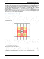
Let us assume for the purpose of this example that in addition to the initial root grid grids (having 128 grid cells along
each axis) there are two subgrids, each of which is half the size of the one above it in each spatial direction (so subgrid
1 spans from 0.25-0.75 in units of the box size and subgrid 2 goes from 0.375-0.625 in each direction). If each grid
is twice as highly refined spatially as the one above it, the dark matter particles on that level are 8 times smaller, so
the dark matter mass resolution on grid #2 is 64 times better than on the root grid, while the total number of initial
grid cells only increases by a factor of three (since each grid is half the size, but twice as highly refined as the one
above it, the total number of grid cells remains the same). Note: See the page on generating initial conditions for more
information on creating this sort of set of nested grids.
20
Chapter 2. Getting Started with Enzo
Enzo Documentation, Release 2.4
When a simulation with more than one initial grid is run, the total number of initial grids
is specified by setting CosmologySimulationNumberOfInitialGrids.
The parameter CosmologySimulationGridDimension[#] is an array of three integers setting the
grid dimensions of each nested grid,
and CosmologySimulationGridLeftEdge[#] and
CosmologySimulationGridRightEdge[#] specify the left and right edges of the grid spatially, in
units of the box size. In the last three parameters, “#” is replaced with the grid number. The root grid is grid 0. None
of the previous three parameters need to be set for the root grid. For the setup described above, the parameter file
would be set as follows:
CosmologySimulationNumberOfInitialGrids = 3
CosmologySimulationGridDimension[1] = 128 128 128
CosmologySimulationGridLeftEdge[1] = 0.25 0.25 0.25
CosmologySimulationGridRightEdge[1] = 0.75 0.75 0.75
CosmologySimulationGridLevel[1] = 1
CosmologySimulationGridDimension[2] = 128 128 128
CosmologySimulationGridLeftEdge[2] = 0.375 0.375 0.375
CosmologySimulationGridRightEdge[2] = 0.625 0.625 0.625
CosmologySimulationGridLevel[2] = 2
Multiple initial grids can be used with or without AMR being turned on. If AMR is used, the parameter
MinimumOverDensityForRefinement must be modified as well. It is advisable to carefully read the entry
for this parameter in the parameter list (in this section). The minimum overdensity needs to be divided by r(d*l) , where
r is the refinement factor, d is the dimensionality, and l is the zero-based highest level of the initial grids. So if we
wish for the same values for MinimumOverDensityForRefinement used previous to apply on the most highly
refined grid, we must divide the set values by 2(3*2) = 64. In addition, one should only refine on the highest level, so
we must reset RefineRegionLeftEdge and RefineRegionRightEdge. The parameters would be reset as
follows:
RefineRegionLeftEdge = 0.375 0.375 0.375
RefineRegionRightEdge = 0.625 0.625 0.625
MinimumOverDensityForRefinement = 0.0625 0.125
A note: When creating multi-level intial conditions, make sure that the initial conditions files for all levels have
the same file name (ie, GridDensity), but that each file has an extension which is an integer corresponding to
its level. For example, the root grid GridDensity file would be GridDensity.0, the level 1 file would be
GridDensity.1, and so forth. The parameters which describe file names (discussed above in the section on initialization parameters) should only have the file name to the left of the period the period (as in a simulation with a single
initial grid), ie,
CosmologySimulationDensityName = GridDensity
Nested Grids and Particles
When initializing a nested grid problem, there can arise an issue of lost particles as a result of running ring. Please see
Particles in Nested Grid Cosmology Simulations for more information.
2.5.6 I/O Parameters
These parameters, defined in more detail in Controlling Enzo data output, control all aspects of Enzo’s data output. One
can output data in a cosmological simulation in both a time-based and redshift-based manner. To output data regularly
in time, one sets dtDataDump to a value greater than zero. The size of this number, which is in units of Enzo’s internal time variable, controls the output frequency. See the Enzo user’s manual section on output format for more information on physical units. Data can be output at specific redshifts as controlled by CosmologyOutputRedshift[#],
where # is the number of the output dump (with a maximum of 10,000 zero-based numbers). The name of the timebased output files are controlled by the parameter DataDumpName and the redshift-based output files have filenames
2.5. Writing Enzo Parameter Files
21
Enzo Documentation, Release 2.4
controlled by RedshiftDumpName. For example, if we want to output data every time the code advances by dt=2.0
(in code units) with file hierarchiess named time_0000, time_0001, etc., and ALSO output explicitly at redshifts
10, 5, 3 and 1 with file hierarchy names RedshiftOutput0000, RedshiftOutput0001, etc., we would set
these parameters as follows:
dtDataDump = 2.0
DataDumpName = time_
RedshiftDumpName = RedshiftOutput
CosmologyOutputRedshift[0] = 10.0
CosmologyOutputRedshift[1] = 5.0
CosmologyOutputRedshift[2] = 3.0
CosmologyOutputRedshift[3] = 1.0
Note that Enzo always outputs outputs data at the end of the simulation, regardless of the settings of dtDataDump
and CosmologyOutputRedshift.
2.5.7 Radiative Cooling and UV Physics Parameters
Enzo comes with multiple ways to calculate baryon cooling and a metagalactic UV background, as described in detail
here. The parameter RadiativeCooling controls whether or not a radiative cooling module is called for each grid.
The cooling is calculated either by assuming equilibrium cooling and reading in a cooling curve, or by computing the
cooling directly from the species abundances. The parameter MultiSpecies controls which cooling module is
called - if MultiSpecies is off (0) the equilibrium model is assumed, and if it is on (1 or 2) then nonequilibrium
cooling is calculated using either 6 or 9 ionization states of hydrogen and helium (corresponding to MultiSpecies
= 1 or 2, respectively). The UV background is controlled using the parameter RadiationFieldType. Currently
there are roughly a dozen backgrounds to choose from. RadiationFieldType is turned off by default, and can
only be used when Multispecies = 1. For example, if we wish to use a nonequilibrium cooling model with a
Haardt and Madau background with qalpha = -1.8, we would set these parameters as follows:
RadiativeCooling = 1
MultiSpecies = 1
RadiationFieldType = 2
2.5.8 Star Formation and Feedback Physics Parameters
Enzo has multiple routines for star formation and feedback. Star particle formation and feedback are controlled
separately, by the parameters StarParticleCreation and StarParticleFeedback. Multiple types of star
formation and feedback can be used, e.g. models for Pop III stars for metal-free gas and models for Pop II stars for
metal-enriched gas. These routines are disabled when these parameters are set equal to 0. These parameters are bitwise
to allow multiple types of star formation routines can be used in a single simulation. For example if methods 1 and 3
are desired, the user would specify 10 (21 + 23 ), or if methods 0, 1 and 4 are wanted, this would be 19 (20 + 21 + 24 ).
See Star Formation and Feedback Parameters for more details.
They are turned on when the i-th bit is flagged. The value of 2 is the recommended value. The most commonly used
routines (2) are based upon an algorithm by Cen & Ostriker, and there are a number of free parameters. Note that it is
possible to turn star particle formation on while leaving feedback off, but not the other way around.
For the star particle creation algorithm, stars are allowed to form only in cells where a minimum overdensity is reached,
as defined by StarMakerOverDensityThreshold. Additionally, gas can only turn into stars with an efficiency
controlled by StarMakerMassEfficiency and at a rate limited by StarMakerMinimumDynamicalTime,
and the minimum mass of any given particle is controlled by the parameter StarMakerMinimumStarMass, which
serves to limit the number of star particles. For example, if we wish to use the “standard” star formation scenario where
stars can only form in cells which are at least 100 times the mean density, with a minimum dynamical time of 106
years and a minimum mass of 107 solar masses, and where only 10% of the baryon gas in a cell can be converted into
stars in any given timestep, we would set these parameters as follows:
22
Chapter 2. Getting Started with Enzo
Enzo Documentation, Release 2.4
StarParticleCreation = 2
StarMakerOverDensityThreshold = 100.0
StarMakerMassEfficiency = 0.1
StarMakerMinimumDynamicalTime = 1.0e6
StarMakerMinimumStarMass = 1.0e7
Star particles can provide feedback into the Inter-Galactic Medium via stellar winds, thermal energy and metal pollution. The parameter StarMassEjectionFraction controls the fraction of the total initial mass of the star particle
which is eventually returned to the gas phase. StarMetalYield controls the mass fraction of metals produced by
each star particle that forms, and StarEnergyToThermalFeedback controls the fraction of the rest-mass energy of the stars created which is returned to the gas phase as thermal energy. Note that the latter two parameters are
somewhat constrained by theory and observation to be somewhere around 0.02 and 1.0e-5, respectively. The ejection
fraction is poorly constrained as of right now. Also, metal feedback only takes place if the metallicity field is turned on
(CosmologySimulationUseMetallicityField = 1). As an example, if we wish to use the ‘standard’ star
feedback where 25% of the total stellar mass is returned to the gas phase, the yield is 0.02 and 10-5 of the rest mass is
returned as thermal energy, we set our parameters as follows:
StarParticleFeedback = 2
StarMassEjectionFraction = 0.25
StarMetalYield = 0.02
StarEnergyToThermalFeedback = 1.0e-5
CosmologySimulationUseMetallicityField = 1
When using the star formation and feedback algorithms it is important to consider the regime of validity of our
assumptions. Each “star particle” is supposed to represent an ensemble of stars, which we can characterize with the
free parameters described above. This purely phenomenological model is only reasonable as long as the typical mass
of the star particles is much greater than the mass of the heaviest stars so that the assumption of averaging over a large
population is valid. When the typical star particle mass drops to the point where it is comparable to the mass of a large
star, these assumptions must be reexamined and our algorithms reformulated.
2.5.9 IO Parallelization Options
One of Enzo’s great strengths is that it is possible to do extremely large simulations on distributed memory machines.
For example, it is possible to intialize a 10243 root grid simulation on a linux cluster where any individual node has
1 or 2 GB of memory, which is on the order of 200 times less than the total dataset size! This is possible because
the reading of initial conditions and writing out of data dumps is fully parallelized - at startup, when the parameter
ParallelRootGridIO is turned on each processor only reads the portion of the root grid which is within its
computational domain, and when ParallelParticleIO is turned on each processor only reads in the particles
within its domain (though preprocessing is needed - see below). Additionally, the parameter Unigrid should be
turned on for simulations without AMR, as it saves roughly a factor of two in memory on startup, allowing the code to
perform even larger simulations for a given computer size. If we wish to perform an extremely large unigrid simulation
with parallel root grid and particle IO, we would set the following parameters:
ParallelParticleIO = 1
ParallelRootGridIO = 1
Unigrid = 1
AMR simulations can be run with ParallelRootGridIO and ParallelParticleIO on, though you must
be careful to turn off the Unigrid parameter. In addition, it is important to note that in the current version
of Enzo you must run the program called “ring” on the particle position and velocity files before Enzo is started
in order to take advantage of the parallel particle IO. Assuming the particle position and velocity files are named
ParticlePositions and ParticleVelocities, respectively, this is done by running:
mpirun -np [N] ring ParticlePositions ParticleVelocities
2.5. Writing Enzo Parameter Files
23
Enzo Documentation, Release 2.4
Where mpirun is the executable responsible for running MPI programs and “-np [N]” tells the machine that there are
[N] processors. This number of processors must be the same as the number which Enzo will be run with!
2.5.10 Notes
This page is intended to help novice Enzo users put together parameter files for their first simulation and therefore is
not intended to be an exhaustive list of parameters nor a complete description of each parameter mentioned. It would
be wise to refer to the Enzo user guide’s Enzo Parameter List for a more-or-less complete list of AMR parameters,
some of which may be extremely useful for your specific application.
2.6 Data Analysis Basics
Data analysis in Enzo can be complicated. There are excellent premade packages available for doing Enzo data
analysis. However, it is likely that your data analysis needs will grow beyond these tools.
2.6.1 HDF5 Tools
Enzo reads in initial conditions files and outputs simulation data using the HDF5 structured data format (created and
maintained by the NCSA HDF group). Though this format takes a bit more effort to code than pure C/C++ binary
output, we find that the advantages are worth it. Unlike raw binary, HDF5 is completely machine-portable and the
HDF5 library takes care of error checking. There are many useful standalone utilities included in the HDF5 package
that allow a user to examine the contents and structure of a dataset. In addition, there are several visualization and data
analysis packages that are HDF5-compatible. See the page on Data Vizualization for more information about this. The
NCSA HDF group has an excellent tutorial on working with HDF5.
Note that as of the Enzo 2.0 code release, Enzo still supports reading the HDF4 data format, but not writing to it.
We strongly suggest that new users completely avoid this and use the HDF5 version instead. Enzo’s parallel IO only
works with HDF5, and we are encouraging users migrate as soon as is feasible.
2.6.2 Using YT to Analyze Data
If you have installed YT along with Enzo (as suggested in the build instructions Obtaining and Building Enzo), you
should be able to use it to find halos, examine profiles, prepare plots and handle data directly via physically meaningful
objects. Documentation, a wiki and a mailing list are available for support and assistance with installation and usage
as well as a brief introduction in these documents Analyzing With YT
2.6.3 Analysis with VisIt
Another tool that has a native reader for Enzo data is VisIt, a parallel VTK-based visualization and analysis tool.
From the VisIt Users website:
VisIt is a free interactive parallel visualization and graphical analysis tool for viewing scientific data
on Unix and PC platforms. Users can quickly generate visualizations from their data, animate them
through time, manipulate them, and save the resulting images for presentations. VisIt contains a rich set
of visualization features so that you can view your data in a variety of ways. It can be used to visualize
scalar and vector fields defined on two- and three-dimensional (2D and 3D) structured and unstructured
meshes. VisIt was designed to handle very large data set sizes in the tera- to peta-scale range and yet can
also handle small data sets in the kilobyte range.
24
Chapter 2. Getting Started with Enzo
Enzo Documentation, Release 2.4
The caveat is that as of version 1.11.2, VisIt only understands the original unpacked AMR format. However, the
packed-AMR is in the VisIt development version, and will be included in the next release (1.12). If would like this
functionality sooner, it’s not too much work. Here’s how to begin:
1. Download the following:
• The 1.11.2 source distribution
• The 1.11.2 build_visit script
• An updated avtEnzoFileFormat.C
• An updated avtEnzoFileFormat.h
2. Untar the source tar file,
3. replace the two files named avtEnzo* in visit1.11.2/src/databases/Enzo/ with the ones you’ve just downloaded,
and
4. retar the file, keeping the same directory structure.
(You can do this without untarring and retarring, but this is a bit clearer for those not familiar with tar.) From this
point, you can build and install VisIt using the build_visit script. When you do this, remember to do two things:
• Use the TARBALL option to specify the tar file for the script to unpack. Failing to do this will cause the script
to download a new tar file, without the changes that you need.
• Select both HDF5 and HDF4 as optional third-party libraries. This may not strictly be necessary, if you
already have HDF5 and HDF4 installed on your system, but the script isn’t clear on how to specify which HDF5
installation to use. (HDF4 needs to be available to satisfy a dependency check for building the Enzo reader.
We’ll ask to have this updated in future versions of VisIt.)
2.6.4 Writing your own tools, I - the Enzo Grid Hierarchy
Enzo outputs each individual adaptive mesh block as its own grid file. Each of these files is completely self-contained,
and has information about all of the grid cells that are within that volume of space. Information on the size and spatial
location of a given grid file can be obtained from the hierarchy file, which has the file extension ”.hierarchy”. This
ascii file has a listing for each grid that looks something like this:
Grid = 26
GridRank
= 3
GridDimension
= 34 22 28
GridStartIndex
= 3 3 3
GridEndIndex
= 30 18 24
GridLeftEdge
= 0.5 0.28125 0.078125
GridRightEdge
= 0.71875 0.40625 0.25
Time
= 101.45392321467
SubgridsAreStatic = 0
NumberOfBaryonFields = 5
FieldType = 0 1 4 5 6
BaryonFileName = RedshiftOutput0011.grid0026
CourantSafetyNumber
= 0.600000
PPMFlatteningParameter = 0
PPMDiffusionParameter = 0
PPMSteepeningParameter = 0
NumberOfParticles
= 804
ParticleFileName = RedshiftOutput0011.grid0026
GravityBoundaryType = 2
Pointer: Grid[26]->NextGridThisLevel = 27
2.6. Data Analysis Basics
25
Enzo Documentation, Release 2.4
GridRank gives the dimensionality of the grid (this one is 3D), GridDimension gives the grid size in grid
cells, including ghost zones. GridStartIndex and GridEndIndex give the starting and ending indices of
the non-ghost zone cells, respectively. The total size of the baryon datasets in each grid along dimension i is (1+
GridEndIndex[i] - GridStartIndex[i]). GridLeftEdge and GridRightEdge give the physical edges
of the grids (without ghost zones) in each dimension. NumberOfParticles gives the number of dark matter particles (and/or star particles, for simulations containing star particles) in a given grid. Note that when there are multiple
grids covering a given region of space at various levels of resolution, particles are stored in the most highly refined
grid. BaryonFileName is the name of the actual grid file, and should be the same as ParticleFileName.
Time is the simulation time, and should be the same as InitialTime in the parameter file for the same data dump.
The other parameters for each entry are more advanced and probably not relevant for simple data analysis.
Possibly the greatest source of potential confusion in Enzo’s datasets is the overlap of grid cells. In a simulation, when
a given grid is further refined, the coarse cells which have not been refined are still kept. The solution to the hydro
and gravity equations are still calculated on that level, but are updated with information from more highly refined
levels. What this is means is that a volume of space which has been refined beyond the root grid is covered by multiple
grid patches at different levels of resolution. Typically, when doing analysis you only want the most highly refined
information for a given region of space (or the most highly refined up to a certain level) so that you don’t double-count
(or worse) the gas in a given cell. Look at this example analysis code.
2.6.5 Writing your own tools, II - Enzo Physical Units
Yet another significant source of confusion is the units that Enzo uses. When doing a cosmology simulation, the code
uses a set of units that make most quantities on the order of unity (in principle). The Enzo manual section on the
code output format Enzo Output Formats explains how to convert code units to cgs units. However, there are some
subtleties:
Density fields All density fields are in the units described in the AMR guide except electron density. Electron density
is only output when MultiSpecies is turned on, and in order to convert the electron density to cgs it must
be multiplied by the code density conversion factor and then (m:sub:e/m:sub:p), where m:sub:eand m:sub:pare
the electron and proton rest masses (making electron density units different from the other fields by a factor of
m:sub:e/m:sub:p). The reason this is done is so that in the code the electron density can be computed directly
from the abundances of the ionized species.
Energy fields There are two possible energy fields that appear in the code - Gas energy and total energy. Both are in
units of specific energy, ie, energy per unit mass. When Zeus hydro is being used (HydroMethod = 2, there
should be only one energy field - “total energy”. This is a misnomer - the Zeus hydro method only follows the
specific internal (ie, thermal) energy of the gas explicitly. When the total energy is needed, it is calculated from
the velocities. When PPM is used (HydroMethod = 0) the number of energy fields depends on whether or
not DualEnergyFormalism is turned on or off. If it is ON (1), there is a “gas energy” field and a “total
energy” field, where “gas energy” is the specific internal energy and “total energy” is “gas energy” plus the
specific kinetic energy of the gas in that cell. If DualEnergyFormalism is OFF (0), there should only be
“total energy”, which is kinetic+internal specific energies. Confused yet?
Particle mass field Particle “masses” are actually stored as densities. This is to facilitate calculation of the gravitational potential. The net result of this is that, in order to calculate the stored particle “mass” to a physical mass,
you must first multiply this field by the volume of a cell in which the particle resides. Remember that particle
data is only stored in the most refined grid that covers that portion of the simulational volume.
When the simulation is done, Enzo will display the message “Successful run, exiting.” Enzo is a complicated code,
with a similarly complicated output format. See the Enzo User Guide page on the Enzo output format Enzo Output
Formats for more information on the data outputs.
Congratulations! If you’ve made it this far, you have now successfully run a simulation using Enzo!
26
Chapter 2. Getting Started with Enzo
Enzo Documentation, Release 2.4
2.6.6 Example Data and Analysis
The sample data generated by this simulation is available online. You can use it as sample data for the the YT tutorial.
2.7 Controlling Enzo data output
How and when Enzo outputs data is described below. There are five ways to control when data is output, two output
formats, and two pitfalls when determining how to output data from your Enzo simulation.
2.7.1 Data Formats and Files
There are two output formats for Enzo data. In both cases, each data dump gets its own directory.
Each data dump writes several key files. NNNN denotes the dump number (i.e. 0001) and basename is something like
RedshiftOutput or data or DD}.
All output files are also restart files. It’s not necessarily wise to write in 32 bit format if you’re computing in 64,
though, as you’ll lose all the extra precision when you restart. (These are makefile flags.)
basenameNNNN:
The parameter file. This contains general simulation parameters,
dump time, cycle, and all the parameters defined here. It's worth
your time to be familiar with what's in this file.
basenameNNNN.hierarchy:
The hierarchy file in text format. Contains a description of the hierarchy. One
entry for each grid, including information like the Grid Size, the
position in the volume, it's position in the hierarchy.
basenameNNNN.boundary:
A description of the boundary (plain text.) Basically a meta
description and filename for the next file
basenameNNNN.boundary.hdf5:
Actually contains the boundary information.
basenameNNNN.harrays:
The hierarchy of grids stored in HDF5 binary format.
Packed AMR
This is the default output format. Each processor outputs all the grids it owns. In addition to the parameter, hierarchy, and boundary files which may or may not be described elsewhere, data is output in one basenameNNNN.taskmapCCCC} file for each processor, which contains a map between grid number and HDF5 file, and
one basenameNNNN.cpuCCCC for each processor NNNN and CCCC are the dump number and cpu number, respectively.
basenameNNNN.cpuCCCC is an HDF5 file which contains an HDF5 group for each grid. Each grid in turn contains
a dataset for each of the fields in the simulation.
2.7. Controlling Enzo data output
27
Enzo Documentation, Release 2.4
~/DD0100>h5ls data0100.cpu0003
Grid00000002
Group
Grid00000026
Group
~/DD0100>h5ls data0100.cpu0003/Grid00000002
Density
Dataset {16, 16, 32}
z-velocity
Dataset {16, 16, 32}
2.7.2 Pathnames
In previous versions of Enzo, the fully-qualified path to each file was output in the .hierarchy file, which requires
modifying the .hierarchy file every time the data was moved. This has changed to be only the relative path to each
data file, which largely eliminates the problem. To restore the old behavior, examine the parameters GlobalDir and
LocalDir.
2.7.3 Timing Methods
There are 6 ways to trigger output from Enzo.
Cycle Based Output
CycleSkipDataDump = N
CycleLastDataDump = W
DataDumpName = data
One can trigger output every N cycles starting with cycle W using CycleSkipDataDump and CycleLastDataDump.
Outputs are put in the directory DD0000 (or DD0001, etc.) and the basename is determined by DataDumpName.
CycleSkipDataDump <= 0 means cycle based output is skipped. The default is 0.
Pitfall 2: CycleLastDataDump defaults to zero and is incremented by CycleSkipDataDump every time output is done.
If you change the value of CycleSkipDataDump and neglect to change CycleLastDataDump, Enzo will dump as long
as CycleNumber >= CycleSkipDataDump + CycleLastDataDump. (So if you change CycleSkipDataDump from 0 to
10 from a Redshift dump at n=70, you’ll get an output every timestep for 7 timesteps.)
Time Based Output
TimeLastDataDump = V
dtDataDump = W
Exactly like Cycle based output, but triggered whenever time >= TimeLastDataDump + dtDataDump. The same pitfall
applies.
Redshift Based Output
CosmologyOutputRedshift[ 0 ] = 12
CosmologyOutputRedshiftName[ 0 ] = Redshift12
RedshiftDumpName
= RedshiftOutput
Outputs at the specified redshift. Any number of these can be specified.
CosmologyOutputRedshift[ i ] is the only necessary parameter, and is the ith redshift to output.
28
Chapter 2. Getting Started with Enzo
Enzo Documentation, Release 2.4
Any outputs with CosmologyOutputRedshiftName[ i ] specified has that name used for the output, and no number is
appended. (so if CosmologyOutputRedshiftName[ 6 ] = BaconHat, the outputs will be BaconHat, BaconHat.hierarchy,
etc.)
If CosmologyOutputRedshiftName[ i ] is omitted, RedshiftDumpName is used for the basename, and the output
number is taken from the array index. (So CosmologyOutputRedshift[19] = 2.34 and RedshiftDumpName = MonkeyOnFire, at dump will be made at z=2.34 with files called MonkeyOnFire0019.hierarchy, etc.)
Force Output Now
The following two options are run time driven. These are especially useful for very deep simulations that spend the
majority of their time on lower levels. Note that unless you have the parameter FileDirectedOutput turned on,
these will not be available.
To force an output as soon as the simulation finished the next step on the finest resolution, make a file called outputNow:
touch outputNow
This will remove the file as soon as the output has finished.
Sub Cycle Based Output
To get the simulation to output every 10 subsycles (again at the finest level of resolution) put the number of subcycles
to skip in a file called subcycleCount:
echo 10 > subcycleCount
Time Based Interpolated Output
Even when you are running simulations with a long dtDataDump, sometimes you may want to see or analyze the
interim datadumps. Using dtInterpolatedDataDump, you can control Enzo to check if it should start outputting interpolated data based on the time passed (dtInterpolatedDataDump < dtDataDump).
dtDataDump = 1e-4
dtInterpolatedDataDump = 1e-5
This is mostly for making movies or looking at the interim data where the TopGrid dt is too long, and in principle, this
output shouldn’t be used for restart.
2.7.4 Friendly Note on Data Output
Enzo is content to output enough data to fill up a hard drive – for instance, your home directory. This should be
noted before output parameters are set, particularly the Sub Cycle outputs, as Enzo has no prohibition against causing
problems with quotas and file system size.
2.7. Controlling Enzo data output
29
Enzo Documentation, Release 2.4
30
Chapter 2. Getting Started with Enzo
CHAPTER 3
User Guide
This document provides a brief description of the compilation and operation of Enzo, a structured Adaptive Mesh
Refinement (SAMR, or more loosely AMR) code which is primarily intended for use in astrophysics and cosmology.
The User’s Guide is intended to explain how to compile and run Enzo, the initial conditions generation code and the
various analysis tools bundled with Enzo. The instructions on actually running the code are not comprehensive in
that they are not machine or platform-specific. Arguably the most useful and important piece of this guide is Enzo
Parameter List, which contains descriptions of all of the roughly 300 possible input parameters (as of September
2008). For more detailed information on the Enzo algorithms and on running Enzo on different platforms, you should
refer to the Getting Started with Enzo. Detailed information on the algorithms used in Enzo will be available in the
method paper (unreleased as of September 2008). In the meantime, see the Enzo Primary References for more concrete
Enzo information.
This guide (and Enzo itself) was originally written by Greg Bryan. Since the original writing of both the simulation
code and the User’s Guide, the maintenance of Enzo and its associated tools and documentation was for some time
largely driven by the Laboratory for Computational Astrophysics at The University of California, San Diego, but it
is now a fully open source community with developers from Stanford, Columbia, Princeton, UCSD, University of
Colorado, Michigan State, UC Berkeley, and many other universities. Your input in improving both the code and the
User’s Guide is appreciated – developement of the code is driven by working researchers, and we encourage everyone
who has made useful changes to contribute those changes back to the community and to participate in the collaborative
development of the code. Email inquiries and comments should be directed to the Enzo Users’ List. Thank you!
3.1 Executables, Arguments, and Outputs
This page is a summary of all of the binaries that are created after make; make install is run in the Enzo code
bundle. They should be located in the bin directory. Links to the various pages of the manual that describe a particular
binary are also included.
3.1.1 enzo
This is the main simulation code executable. See Running Enzo for more detailed information.
When an Enzo simulation is run, at every datastep several files are output, inserted into subdirectories. The most
important of these are the files with no extension and those ending in .hierarchy, of which there will be one of
each for each datadump. For more information on the format of Enzo output, see Enzo Output Formats.
usage: ./enzo.exe [options] param_file
options are:
-d(ebug)
-r(estart)
31
Enzo Documentation, Release 2.4
-x(extract)
-l(evel_of_extract) level
-p(roject_to_plane) dimension
-P(roject_to_plane version 2) dimension
-m(smooth projection)
-o(utput as particle data)
-g (Write Potential field only)
-M (Write smoothed DM field only)
-F(riends-of-friends halo finder only)
-C(ooling time write only)
-h(elp)
-i(nformation output)
-V (show compiler options and flags)
-s(tart index region) dim0 [dim1] [dim2]
-e(nd
index region) dim0 [dim1] [dim2]
-b(egin coordinate region) dim0 [dim1] [dim2]
-f(inish coordinate region) dim0 [dim1] [dim2]
The -g, -M, and -C flags will read in the dataset given on the command line and write additional data fields to the same
data files. When running with these flags (or the -F flag), the -r flag must also be given so that the code knows to read
in a dataset. For example, to write out the cooling time to the output DD0001, do the following:
enzo.exe -r -C DD0001/DD0001
3.1.2 inits
This is the initial conditions generator. See Using inits for more detailed information. Initial conditions with a single
initial grid or multiple nested grids can be created with this executable. Output file names are user-specified, but in a
standard cosmology simulation with a single initial grid there should be a file containing baryon density information,
another containing baryon velocity information, and two more files containing particle position and velocity information. Simulations with multiple grids will have a set of these files for each level, appended with numbers to make them
unique.
usage: inits [options] param_file
options are:
-d(ebug)
-s(ubgrid) param_file
3.1.3 ring
ring must be run on the simulation particle position and velocity information before a simulation is executed when
the Enzo runtime parameter ParallelParticleIO is set to 1. Running ring generates files called PPos.nnnn
PVel.nnnn where nnnn goes from 0001 to the total number of processors that are used for the simulation. These
files contain the particle position and velocity information for particles that belong to each processor individually, and will be read into the code instead of the monolithic particle position and velocity files. Note that if
ParallelParticleIO is on and ring is NOT run, the simulation will crash.
usage:
ring [string] <particle position file> <particle velocity file>
[string] can be one of the following: pv, pvm, pvt, or pvmt. p, v, m and t correspond to position, velocity, mass, and
type, respectively. The most common [string] choice is ‘pv’. In that case, and if you use the default names for the
particle position and velocity files, your usage will look like:
ring pv ParticlePositions ParticleVelocities
32
Chapter 3. User Guide
Enzo Documentation, Release 2.4
3.1.4 enzohop
The second (and generally favored) method used for finding density peaks in an Enzo simulation. More information
can be found here. A file called HopAnalysis.out is output which contains halo position and mass information.
enzohop [-b #] [-f #] [-t #] [-g] [-d] amr_file
-b)egin region
-f)inish region
-t)hreshold for hop (default 160)
-g)as particles also used (normally just dm)
-d)ebug
3.1.5 anyl
anyl is the analysis package written in C, previously known as enzo_anyl. Although the analysis toolkit for enzo
that’s being constantly updated is YT, anyl has its own value for some users. It creates radial, disk, vertical profiles
for baryon (each species), dark matter, and star particles. Works with all AMR formats including HDF4 and packed
HDF5.
usage: anyl.exe <amr file> <anyl parameter file>
3.2 Running Enzo
Once the code is compiled and a parameter file is prepared, starting the simulation is easy:
mpirun -np 1 enzo [-d] parameter_file
The syntax of the mpirun varies between mpi implementations. The example given here comes from a machine using
a standard MPI implementation that is initiated by the ‘mpirun’ command, and implies the use of a single processors
(the argument after the -np flag indicates the number of processors).
The -d flag triggers a debug option that produces a substantial amount of output. See Getting Started with Enzo for
more detailed information on running simulations. You may also need to use ring if you are using parallel I/O.
3.2.1 Restarting
During a run, there are a number of forms of output. The largest will probably be the output of the full dataset as
specified by parameters such as dtDataDump and the CosmologyOutputRedshift. Such outputs contain a
number of different files (sometimes many files if there are a large number of grids) and are explained elsewhere. It
is useful to have a fairly large number of such outputs if the run is a long one, both to provide more information to
analyze, but also in case of an unintended interruption (crash). Fortunately, any full output can be used to restart the
simulation:
mpirun -np 1 enzo [-d] -r output_name
3.2.2 Monitoring information
As the simulation runs, at every top grid timestep, it outputs a line of information to the ascii file OutputLevelInformation (which is overwritten on restart). The amount of information on this line can be quite extensive, but here the
format is briefly summarized. The first number is the problem time, while the next 6 relate to general information
about the entire run. Within these six numbers, the first is the maximum level currently in use, the second is the
3.2. Running Enzo
33
Enzo Documentation, Release 2.4
number of grids, the third is a number proportional to the memory used, the fourth is the mean axis ratio of all grids,
and the last two are reserved for future use. Then, there are three spaces, and another group of numbers, all providing
information about the first (top grid) level. This pattern of three spaces and six numbers is repeated for every level. An
example of this file is provided below.
Cycle 151 Time 20.241365 MaxDepth 4 Grids 412 Memory(MB) 53.3117 Ratio 2.22582
Level 0 Grids 2 Memory(MB) 13.8452 Coverage 1 Ratio 2 Flagged 0 Active 262144
Level 1 Grids 304 Memory(MB) 31.4977 Coverage 0.166855 Ratio 2.43768 Flagged 0 Active 349920
Level 2 Grids 76 Memory(MB) 5.81878 Coverage 0.00329208 Ratio 1.66118 Flagged 0 Active 55232
Level 3 Grids 22 Memory(MB) 1.74578 Coverage 0.000125825 Ratio 1.63561 Flagged 0 Active 1688
Level 4 Grids 8 Memory(MB) 0.404286 Coverage 2.5034e-06 Ratio 1.21875 Flagged 0 Active 2688
The information for each level is:
1. number of grids on the level
2. memory usage (minus overhead). Actual memory usage is usually a factor of 10 higher.
3. the volume fraction of the entire region covered by grids on this level,
4. the mean axis ratio of grids on this level
5. the fraction of cells on this level which need refinement (unused)
6. the number of active cells on this level.
3.2.3 Debugging information
It is often useful to run with the debug flag turned on, particularly if the code is crashing for unknown reasons.
However, the amount of output is quite large so it is useful to redirect this to a log file, such as:
mpirun -np 1 enzo -d -r output_name >& log_file
Some modules (the cooling unit is particularly bad for this), produce their own debugging logs in the form of fort.??
files. These can be ignored unless problems occur.
3.2.4 Test Problems
There are a number of built-in tests, which can be used to debug the system or characterize how well it solves a particular problem. (see Enzo Test Suite for a complete list.) Note that Enzo can run any problem after compilation, since no
compilation flags affect simulation parameters. To run a particular test, cd to the [browser:public/trunk/doc/examples
doc/examples] subdirectory of the Enzo source distribution (after compiling enzo) and use the following commandline:
mpirun -np 1 enzo [-d] test_name
The syntax of the mpirun various from mpi implementation. The example given here comes from the Origin2000 and
implies a single processor (the argument after the -np flag indicates the number of processors).
The parameter test_name corresponds to the parameter file that specifies the type of test and the test particulars. This
file is ascii, and can be edited. It consists of a series of lines (and optional comments) each of which specifies the value
of one parameter. The parameters are discussed in more detail in Enzo Parameter List.
If you just type enzo without any arguments, or if the number of arguments is incorrect, the program should respond
with a summary of the command-line usage.
The -d flag turns on a rather verbose debug option.
For example, to run the shock tube test, use:
34
Chapter 3. User Guide
Enzo Documentation, Release 2.4
mpirun -np 1 enzo ShockTube
or
enzo ShockTube
The response should be:
Successfully read in parameter file ShockTube.
Successful completion...
How do you know if the results are correct? New for v2.0, we have added more regression tests and answer tests, using
LCAtest. We hope to add more answer tests, especially for large production-type simulations, e.g. a 5123 cosmology
simulation.
3.3 Measuring Simulation Progress
Measuring the progress of an Enzo simulation can be tricky as each level of the hierarchy has its own timestep and a lot
of information is printed. Fortunately, the Enzo source comes with its own progress meter which provides a great deal
of useful information on the state of a simulation. The progress meter is called np and is located in the bin directory
of the Enzo source.
3.3.1 Running Enzo with the Progress Meter
To get the most out of the progress meter, simulations should be run with the -d flag (for debug output) and have both
the standard output and standard error piped into a single file. Note, running Enzo with -d will not slow down the
simulation. In a bash environment, the standard output and error can be piped into the same file in the following way:
[mpirun ...] ./enzo.exe -d AMRCosmology.enzo >& estd.out
3.3.2 Using the Progress Meter
To use the progress meter, simply run it from within the simulation directory.
~ ./np -t "AMRCosmology" -l 5
+----------------------------------------- AMRCosmology -----------------------------------------+
| Sat Oct 26 01:20:00 1985
Status: 30.996% complete.
|
+------------------- Time ------------------+ +-------------------- Output ----------------------+
| Initial | Current |
Final
| Units | |
|
Time
| Redshift | Name | Completed |
+-----------+-----------+-----------+-------+ +------+-----------+----------+--------+-----------|
| 8.163e-01 | 7.175e+01 | 2.297e+02 | code | | Last | 7.082e+01 | 1.558275 | DD0014 | ------- |
| 4.911e+07 | 4.316e+09 | 1.382e+10 | years | | Next | 7.582e+01 | 1.438446 | DD0015 | 18.61270% |
+-------------------------------------------+ +--------------------------------------------------+
+--------------------------- Hierarchy --------------------------+ +--------- Redshift ----------+
| L | Grids | Volume
|
dt
| Sub | Completed | Iter |R| | Initial | Current | Final |
+---+-------+-----------+-----------+-------+-----------+------+-+ +---------+---------+---------+
| 0 |
4 | 1.000e+00 | 2.021e+00 | 1.000 | 1.0000000 | 159 | | | 50.0000 | 1.53496 | 0.00000 |
| 1 |
49 | 1.500e-01 | 6.820e-01 | 0.688 | 0.6879505 |
54 | | +-----------------------------+
| 2 |
16 | 4.997e-03 | 2.297e-01 | 0.337 | 0.4641940 |
67 | |
| 3 |
9 | 1.779e-04 | 9.501e-02 | 1.000 | 0.4641943 | 150 | |
| 4 |
4 | 3.755e-06 | 9.501e-02 | 1.000 | 0.4641941 | 271 | |
| 5 |
1 | 2.012e-07 | 2.852e-02 | 0.919 | 0.4603860 | 457 |<|
+----------------------------------------------------------------+
+---------------------------------------------
3.3. Measuring Simulation Progress
35
Enzo Documentation, Release 2.4
| TransferSubgridParticles[5]: Moved 0 particles, 0 stars.
| DetermineSGSize: MaxSubgridSize = 2000, MinSubgridEdge = 4, ncells = 216
| RebuildHierarchy[5]: Flagged 0/1 grids. 0 flagged cells
| Level[5]: dt = 0.0285228 0.0285228 (0.0873183/0.0950141)
| RebuildHierarchy: level = 5
+---------------------------------------------
The progress meter will continue to update automatically as more information is written to the log file.
3.3.3 Progress Meter Output
The progress meter has four section: time, output, hierarchy, and redshift (if a cosmology simulation.) The time section
gives the initial, current, and final time in both code units and years. The redshift section gives the initial, current, and
final redshift of the simulation. The output section gives the time, redshift, and names of the previous and next data
dump as well as the percentage that the simulation is to reaching the next output. The hierarchy section displays, for
each level of the hierarchy, the number of grids, the total volume of grids, the current timestep, the completion fraction
of the level above, the completion fraction of the root grid timestep, and the number of iterations taken. The far right
column shows what level is being computed and the current status. See below for an explanation of the symbols. If
the -l flag is given, an additional section will appear with the last lines written to the log file.
3.3.4 Additional Options
Additional options can be seen by running the progress meter with the -h flag.
~ ./np -h
np:
-h: print this help output.
-d <directory>: simulation directory (default: .).
-hf <filename>: hierarchy file (default: OutputLevelInformation.out).
-l <number of output lines>: print enzo standard out lines (default: 0).
-of <filename>: enzo standard out file (default: estd.out).
-ol <filename>: enzo output log file (default: OutputLog).
-pf <filename>: parameter file (default: amr.out).
-t <title>: title of simulation.
-w <seconds>: change number of seconds between output (default: 1).
Status:
E: Evolve Level
R: Rebuild Hierarchy
W: Writing Data
.: Evolve Level Complete
3.4 Running Enzo with CUDA
Enzo contains CUDA version of PPM and MHD solver. Supported parameters include
• PPM: TwoShock, HLL, HLLC, PPMFlatteningParameter, PPMSteepeningParameter, DualEnergyFormalism,
RiemannSolverFallback
• MHD: HLL-PLM
• Gravity
• Color fields: chemistry, etc
• Driving field
36
Chapter 3. User Guide
Enzo Documentation, Release 2.4
• Comoving coordinates
• EOSType: 0
3.4.1 How to compile with CUDA
In order to make Enzo compatible with CUDA, a few changes need to be made in the settings.
Currently Enzo CUDA is only compatible with 32-bit precision. In order to correctly set this, make sure that in
src/enzo/ you run the following configuration commands:
:: make cuda-yes make integers-32 make precision-32 make particles-32 make particle-id-32 make inits-32 make
io-32
Then locate your machine specific Makefile, e.g. Make.mach.mymach, and then set the following variables:
MACH_OPT_CUDA = -arch=sm_20 -03
MACH_LIBS_CUDA = -L/your/cuda/install/dir/lib64 -lcudart
If using the Kepler K20 GPU, then
MACH_OPT_CUDA = -arch=sm_35 -03
Last thing to note is that the CUDA solver is single precision only. Check to make sure that all the precision flags are
set correctly. For example,
MACH_FFLAGS_INTEGER_32 =
MACH_FFLAGS_INTEGER_64 = -i8
MACH_FFLAGS_REAL_32 =
MACH_FFLAGS_REAL_64 = -r8
3.4.2 How to run with CUDA
The only thing to do is to set UseCUDA=1 in whichever parameter file. That’s all!
Be sure that each node has at least 1 NVIDIA GPU. Also note that each GPU can be running multiple MPI processes,
the performance will typically increase with mulitple MPI processes per GPU. So it’s recommended to set the number
of MPI processes per node to be the number of CPU cores to fully use both the CPU and GPU resources. Furthermore,
on Kepler K20 GPU, it’s recommended to turn on CUDA MPS (Multi-Process Service), which enables concurrent
running of multiple MPI processes on the GPU.
3.5 Running Enzo with Grackle
The Grackle is an external chemistry and cooling library originally derived from Enzo’s MultiSpecies chemistry and
Cloudy cooling modules. The non-equilibrium primordial chemistry and cooling functionality is essentially identical to the MultiSpecies network. However, significant updates have been made to the treatment of metals and UV
backgrounds that may make using the Grackle a more attactive option, such as:
• UV backgrounds are treated via interpolating from data tables loaded from disk rather than piece-wise polynomial functions, making it somewhat easier to add support for new background models.
• UV background and cooling data are contained within the same input file and are more consistent than the
currently available Cloudy cooling data and Enzo UV background models. Currently, the Grackle distribution
comes with UV background and cooling data for two different models:
1. Faucher-Giguere et al. (2009).
3.5. Running Enzo with Grackle
37
Enzo Documentation, Release 2.4
2. Haardt & Madau (2012).
• Unlike the original Cloudy cooling which required separate input files for cooling before the UV background
turns on and after, all data is contained in a single table. This means one no longer has to run with one input file
to the redshift where the UV background starts, stop the simulation, and restart with another input file.
• Also unlike the original Cloudy cooling module, Grackle supports the option to also solve the primordial cooling
via interpolation from a table. Thus, one is no longer required to run with the MultiSpecies functionality in order
to calculate the primordial component. This simplified method is somewhat faster and requires fewer baryon
fields to be stored, lowering the ram and disk footprint.
For more information on the Grackle library, see the Grackle documentation.
3.5.1 Obtaining and Building the Grackle
See the Grackle documentation for complete instruction on how to obtain, compile, and install the Grackle library.
3.5.2 Compiling Enzo with Grackle
In order to compile Enzo with support for Grackle, the following lines need to be added to your machine make file in
the appropriate places:
LOCAL_GRACKLE_INSTALL = PATH/TO/GRACKLE
LOCAL_INCLUDES_GRACKLE = -I$(LOCAL_GRACKLE_INSTALL)/include
MACH_INCLUDES_GRACKLE = $(LOCAL_INCLUDES_GRACKLE)
LOCAL_LIBS_GRACKLE = -L$(LOCAL_GRACKLE_INSTALL)/lib -lgrackle
MACH_LIBS_GRACKLE = $(LOCAL_LIBS_GRACKLE)
See the example make file, Make.mach.unkown, in the Enzo source for an example.
To configuration Enzo to build with Grackle support, do the following before typing “make”:
make grackle-yes
3.5.3 Running with the Grackle
Grackle parameters should be given in the same parameter file as the rest of the Enzo parameters. Since the Grackle
is based on Enzo’s MultiSpecies, many of the parameter names are the same. For a full list of Grackle parameters, see
here.
3.6 Enzo Test Suite
The Enzo test suite is a set of tools whose purpose is to perform regression tests on the Enzo codebase, in order to
help developers discover bugs that they have introduced, to verify that the code is producing correct results on new
computer systems and/or compilers, and, more generally, to demonstrate that Enzo is behaving as expected under a
wide variety of conditions.
3.6.1 What’s in the test suite?
The suite is composed of a large number of individual test problems that are designed to span the range of physics and
dimensionalities that are accessible using the Enzo code, both separately and in various permutations. Tests can be
selected based on a variety of criteria, including (but not limited to) the physics included, the estimated runtime of the
38
Chapter 3. User Guide
Enzo Documentation, Release 2.4
test, and the dimensionality. The testing suite runs enzo on each selected test problem, produces a series of outputs,
and then uses yt to process these outputs in a variety of different ways (making projections, looking at fields, etc.). The
results of these yt analyses are then compared against similarly generated results from an earlier “good” version of the
enzo code run on the same problems. In test problems where we have them, analytical solutions are compared against
the test results (e.g. shocktubes). Lastly, a summary of these test results are returned to the user for interpretation.
One can run individual tests or groups of tests using the various run time flags. For convenience, three pre-created,
overlapping sets of tests are provided. For each set of tests, one must generate their own standard locally against which
she can compare different builds of the code.
1. The “quick suite” (--suite=quick). This is composed of small calculations that test critical physics packages
both alone and in combination. The intent of this package is to be run automatically and relatively frequently (multiple
times a day) on a remote server to ensure that bugs have not been introduced during the code development process.
All runs in the quick suite use no more than a single processor. The total run time should be about 15 minutes on the
default lowest level of optimization..
2. The “push suite” (--suite=push). This is a slightly large set of tests, encompassing all of the quick suite and
some additional larger simulations that test a wider variety of physics modules. The intent of this package is to provide
a thorough validation of the code prior to changes being pushed to the main repository. The total run time is roughly
60 minutes for default optimization, and all simulations use only a single processor.
3. The “full suite” (--suite=full). This encompasses essentially all of test simulations contained within the
run directory. This suite provides the most rigorous possible validation of the code in many different situations, and is
intended to be run prior to major changes being pushed to the stable branch of the code. A small number of simulations
in the full suite are designed to be run on 2 processors and will take multiple hours to complete. The total run time is
roughly 60 hours for the default lowest level of optimization.
3.6.2 How to run the test suite
1. Compile Enzo. If you have already built enzo, you can skip this step and the test will use your existing enzo
executable. To compile enzo with the standard settings, complete these commands:
$
$
$
$
cd <enzo_root>/src/enzo
make default
make clean
make
Note that you need not copy the resulting enzo executable to your path, since the enzo.exe will be symbolically linked
from the src/enzo directory into each test problem directory before tests are run.
2. Get the correct yt version The enzo tests are generated and compared using the yt analysis suite. You must be
using yt 2.6.3 in order for the test suite to work. The test suite has not yet been updated to work with yt 3.0 and newer
releases. If you do not yet have yt, visit http://yt-project.org/#getyt for installation instructions. If you already have yt
and yt is in your path, make sure you’re using yt 2.6.3 by running the following commands:
$ cd /path/to/yt_mercurial_repository
$ hg update yt-2.x
$ python setup.py develop
3. Generate answers to test with. Run the test suite with these flags within the run/ subdirectory in the enzo source
hierarchy:
$ cd <enzo_root>/run
$ ./test_runner.py --suite=quick -o <output_dir> --answer-store
--answer-name=<test_name> --local
Note that we’re creating test answers in this example with the quick suite, but we could just as well create a reference
from any number of test problems using other test problem flags.
3.6. Enzo Test Suite
39
Enzo Documentation, Release 2.4
Here, we are storing the results from our tests locally in a file called <test_name> which will now reside inside of the
<output_dir>. If you want to, you can leave off --answer-name and get a sensible default.
$ ls <output_dir>
fe7d4e298cb2
<test_name>
$ ls <output_dir>/<test_name>
<test_name>.db
When we inspect this directory, we now see that in addition to the subdirectory containing the simulation results, we
also have a <test_name> subdirectory which contains python-readable shelve files, in this case a dbm file. These are
the files which actually contain the reference standard. You may have a different set of files or extensions depending
on which OS you are using, but don’t worry Python can read this no problem. Congratulations, you just produced
your own reference standard. Feel free to test against this reference standard or tar and gzip it up and send it to another
machine for testing.
4. Run the test suite using your local answers. The testing suite operates by running a series of enzo test files
throughout the run subdirectory. Note that if you want to test a specific enzo changeset, you must update to it and
recompile enzo. You can initiate the quicksuite test simulations and their comparison against your locally generated
answers by running the following commands:
$ cd <enzo_root>/run
$ ./test_runner.py --suite=quick -o <output_dir> --answer-name=<test_name>
--local --clobber
In this command, --output-dir=<output_dir> instructs the test runner to output its results to a userspecified directory (preferably outside of the enzo file hierarchy). Make sure this directory is created before you
call test_runner.py, or it will fail. The default behavior is to use the quick suite, but you can specify any set of tests
using the --suite or --name flags. We are comparing the simulation results against a local (--local) reference standard which is named <test_name> also located in the <output_dir> directory. Note, we included the
--clobber flag to rerun any simulations that may have been present in the <output_dir> under the existing enzo
version’s files, since the default behavior is to not rerun simulations if their output files are already present. Because
we didn’t set the --answer-store flag, the default behavior is to compare against the <test_name>.
5. Review the results. While the test_runner is executing, you should see the results coming up at the terminal in real
time, but you can review these results in a file output at the end of the run. The test_runner creates a subdirectory in
the output directory you provided it, as shown in the example below.
$ ls <output_dir>
fe7d4e298cb2
$ ls <output_dir>/fe7d4e298cb2
Cooling
GravitySolver
Cosmology
Hydro
MHD
RadiationTransport
test_results.txt
version.txt
The name of this directory will be the unique hash of the version of enzo you chose to run with the testing suite. In this
case it is fe7d4298cb2, but yours will likely be different, but equally unintelligible. You can specify an optional
additional suffix to be appended to this directory name using --run-suffix=<suffix>. This may be useful to
distinguish multiple runs of a given version of enzo, for example with different levels of optimization. Within this
directory are all of the test problems that you ran along with their simulation outputs, organized based on test type
(e.g. Cooling, AMR, Hydro, etc.) Additionally, you should see a file called test_results.txt, which contains
a summary of the test runs and which ones failed and why.
3.6.3 My tests are failing and I don’t know why
A variety of things cause tests to fail: differences in compiler, optimization level, operating system, MPI submission method, and of course, your modifications to the code. Go through your test_results.txt file for more
40
Chapter 3. User Guide
Enzo Documentation, Release 2.4
information about which tests failed and why. You could try playing with the relative tolerance for error using the
--tolerance flag as described in the flags section. For more information regarding the failures of a specific test,
examine the estd.out file in that test problem’s subdirectory within the <output_dir> directory structure, as it
contains the STDERR and STDOUT for that test simulation.
If you are receiving EnzoTestOutputFileNonExistent errors, it means that your simulation is not completing.
This may be due to the fact that you are trying to run enzo with MPI which your system doesn’t allow you to initiate
from the command line. (e.g. it expects you to submit mpirun jobs to the queue). You can solve this problem by
recompiling your enzo executable with MPI turned off (i.e. make use-mpi-no), and then just pass the local_nompi
machine flag (i.e. -m local_nompi) to your test_runner.py call to run the executable directly without MPI support.
Currently, only a few tests use multiple cores, so this is not a problem in the quick or push suites.
If you see a lot of YTNoOldAnswer errors, it may mean that your simulation is running to a different output than
what was reached for your locally generated answers does, and the test suite is trying to compare your last output file
against a non-existent file in the answers. Look carefully at the results of your simulation for this test problem using
the provided python file to determine what is happening. Or it may simply mean that you specified the wrong answer
name.
3.6.4 Descriptions of all the testing suite flags
You can type ./test_runner.py --help to get a quick summary of all of the command line options for the
testing suite. Here is a more thorough explanation of each.
General flags
-h, --help list all of the flags and their argument types (e.g. int, str, etc.)
-o str, --output-dir=str default: None Where to output the simulation and results file hierarchy. Recommended to specify outside of the enzo source hierarchy.
-m str, --machine=str default: local Specify the machine on which you’re running your tests. This loads up
a machine-specific method for running your tests. For instance, it might load qsub or mpirun in order to start the
enzo executable for the individual test simulations. You can only use machine names of machines which have
a corresponding machine file in the run/run_templates subdirectory (e.g. nics-kraken). N.B. the default,
local, will attempt to run the test simulations using mpirun, so if you are required to queue on a machine
to execute mpirun, test_runner.py will silently fail before finishing your simulation. You can avoid this
behavior by compiling enzo without MPI and then setting the machine flag to local_nompi.
--repo=str default: current directory Path to repository being tested.
--interleave default: False Interleaves preparation, running, and testing of each individual test problem as opposed to default batch behavior.
--clobber default: False Rerun enzo on test problems which already have results in the destination directory
--tolerance=int default: see --strict Sets the tolerance of the relative error in the comparison tests in powers of 10.
Ex: Setting --tolerance=3 means that test results are compared against the standard and fail if they are off
by more than 1e-3 in relative error.
--bitwise default: see --strict Declares whether or not bitwise comparison tests are included to assure that
the values in output fields exactly match those in the reference standard.
--strict=[high, medium, low] default: low This flag automatically sets the --tolerance and
--bitwise flags to some arbitrary level of strictness for the tests. If one sets --bitwise or --tolerance
explicitly, they trump the value set by --strict. When testing enzo general functionality after an installation, --strict=low is recommended, whereas --strict=high is suggested when testing modified code
against a local reference standard.
3.6. Enzo Test Suite
41
Enzo Documentation, Release 2.4
high: tolerance = 13, bitwise = True medium: tolerance = 6, bitwise = False low: tolerance = 3, bitwise =
False
--sim-only default: False Only run simulations, do not store the tests or compare them against a standard.
--test-only default: False Only perform tests on existing simulation outputs, do not rerun the simulations.
--time-multiplier=int default: 1 Multiply simulation time limit by this factor. Useful if you’re on a slow
machine or you cannot finish the specified tests in their allocated time.
--run-suffix=str default: None An optional suffix to append to the test run directory. Useful to distinguish
multiple runs of a given changeset.
-v, --verbose default: False Verbose output in the testing sequence. Very good for tracking down specific test
failures.
--pdb default: False When a test fails a pdb session is triggered. Allows interactive inspection of failed test data.
Flags for storing, comparing against different standards
--answer-store default: False Should we store the results as a reference or just compare against an existing
reference?
--answer-name=str default: latest gold standard The name of the file where we will store our reference results, or if --answer-store is false, the name of the reference against which we will compare our results.
--local default: False Store/Compare the reference standard locally (i.e. not on the cloud)
Bisection flags
-b, --bisect default: False Run bisection on test. Requires revisions --good and --bad. Best if --repo is
different from location of test_runner.py runs --problematic suite.
--good=str default: None For bisection, most recent good revision
--bad=str default: None For bisection, most recent bad revision
-j int, --jcompile=int default: 1 number of processors with which to compile when running bisect
--changeset=str default: latest Changeset to use in simulation repo. If supplied, make clean && make is also
run
Flags not used
--with-answer-testing default: False DO NOT USE. This flag is used in the internal yt answer testing and
has no purpose in the enzo testing infrastructure.
--answer-big-data default: False DO NOT USE. This flag is used in the internal yt answer testing and has no
purpose in the enzo testing infrastructure.
Flags for specifying test problems
These are the various means of specifying which test problems you want to include in a particular run of the testing
suite.
--suite=[quick, push, full] default: None A precompiled collection of several different test problems.
quick: 37 tests in ~15 minutes, push: 48 tests in ~30 minutes, full: 96 tests in ~60 hours.
--answer_testing_script=str default: None
--AMR=bool default: False Test problems which include AMR
--author=str default: None Test problems authored by a specific person
--chemistry=bool default: False Test problems which include chemistry
--cooling=bool default: False Test problems which include cooling
42
Chapter 3. User Guide
Enzo Documentation, Release 2.4
--cosmology=bool default: False Test problems which include cosmology
--dimensionality=[1, 2, 3] Test problems in a particular dimension
--gravity=bool default: False Test problems which include gravity
--hydro=bool default: False Test problems which include hydro
--max_time_minutes=float Test problems which finish under a certain time limit
--mhd=bool default: False Test problems which include MHD
--name=str default: None A test problem specified by name
--nprocs=int default: 1 Test problems which use a certain number of processors
--problematic=bool default: False Test problems which are deemed problematic
--radiation=[None, fld, ray] default: None Test problems which include radiation
--runtime=[short, medium, long] default: None Test problems which are deemed to have a certain predicted runtime
3.6.5 How to track down which changeset caused your test failure
In order to identify changesets that caused problems, we have provided the --bisect flag. This runs hg bisect on
revisions between those which are marked as –good and –bad.
hg bisect automatically manipulates the repository as it runs its course, updating it to various past versions of the code
and rebuilding. In order to keep the tests that get run consistent through the course of the bisection, we recommend
having two separate enzo installations, so that the specified repository (using --repo) where this rebuilding occurs
remains distinct from the repository where the testing is run.
To minimize the number of tests run, bisection is only run on tests for which problematic=True. This must be
set by hand by the user before running bisect. It is best that this is a single test problem, though if multiple tests match
that flag, failures are combined with “or”
An example of using this method is as follows:
$ echo "problematic = True" >> Cosmology/Hydro/AdiabaticExpansion/AdiabaticExpansion.enzotest
$ ./test_runner.py --output-dir=/scratch/dcollins/TESTS --repo=/SOMEWHERE_ELSE
--answer-compare-name=$mylar/ac7a5dacd12b --bisect --good=ac7a5dacd12b
--bad=30cb5ff3c074 -j 8
To run preliminary tests before bisection, we have also supplied the --changeset flag. If supplied, --repo is
updated to --changeset and compiled. Compile errors cause test_runner.py to return that error, otherwise
the tests/bisector is run.
3.6.6 How to add a new test to the library
It is hoped that any newly-created or revised physics module will be accompanied by one or more test problems, which
will ensure the continued correctness of the code. This sub-section explains the structure of the test problem system
as well as how to add a new test problem to the library.
Test problems are contained within the run/ directory in the Enzo repository. This subdirectory contains a tree
of directories where test problems are arranged by the primary physics used in that problem (e.g., Cooling, Hydro,
MHD). These directories may be further broken down into sub-directories (Hydro is broken into Hydro-1D, Hydro2D, and Hydro-3D), and finally into individual directories containing single problems. A given directory contains,
at minimum, the Enzo parameter file (having extension .enzo, described in detail elsewhere in the manual) and the
Enzo test suite parameter file (with extension .enzotest). The latter contains a set of parameters that specify the
3.6. Enzo Test Suite
43
Enzo Documentation, Release 2.4
properties of the test. Consider the test suite parameter file for InteractingBlastWaves, which can be found in the
run/Hydro/Hydro-1D/InteractingBlastWaves directory:
name = 'InteractingBlastWaves'
answer_testing_script = None
nprocs = 1
runtime = 'short'
hydro = True
gravity = False
AMR = True
dimensionality = 1
max_time_minutes = 1
fullsuite = True
pushsuite = True
quicksuite = True
This allows the user to specify the dimensionality, physics used, the runtime (both in terms of ‘short’, ‘medium’, and
‘long’ calculations, and also in terms of an actual wall clock time). A general rule for choosing the runtime value is
‘short’ for runs taking less than 5 minutes, ‘medium’ for run taking between 5 and 30 minutes, and ‘long’ for runs
taking more than 30 minutes. If the test problem runs successfully in any amount of time, it should be in the full suite,
selected by setting fullsuite=True. If the test runs in a time that falls under ‘medium’ or ‘short’, it can be added
to the push suite (pushsuite=True). If the test is ‘short’ and critical to testing the functionality of the code, add it
to the quick suite (quicksuite=True).
Once you have created a new problem type in Enzo and thoroughly documented the parameters in the Enzo parameter
list, you should follow these steps to add it as a test problem:
1. Create a fork of Enzo.
2. Create a new subdirectory in the appropriate place in the run/ directory. If your test problem uses multiple pieces
of physics, put it under the most relevant one.
3. Add an Enzo parameter file, ending in the extension .enzo, for your test problem to that subdirectory.
4. Add an Enzo test suite parameter file, ending in the extension .enzotest. In that file, add any relevant parameters
as described above.
5. By default, the final output of any test problem will be tested by comparing the min, max, and mean of a set
of fields. If you want to have additional tests performed, create a script in the problem type directory and set the
answer_testing_script parameter in the .enzotest file to point to your test script. For an example of
writing custom tests, see run/Hydro/Hydro-3D/RotatingCylinder/test_rotating_cylinder.py.
6. Submit a Pull Request with your changes and indicate that you have created a new test to be added to the testing
suites.
Congratulations, you’ve created a new test problem!
3.6.7 What to do if you fix a bug in Enzo
It’s inevitable that bugs will be found in Enzo, and that some of those bugs will affect the actual simulation results
(and thus the test problems used in the problem suite). Here is the procedure for doing so:
1. Run the “push suite” of test problems (--pushsuite=True) for your newly-revised version of Enzo, and
determine which test problems now fail.
2. Visually inspect the failed solutions, to ensure that your new version is actually producing the correct results!
3. Email the enzo-developers mailing list at [email protected] to explain your bug fix, and to show the
results of the now-failing test problems.
4. Create a pull request for your fix.
44
Chapter 3. User Guide
Enzo Documentation, Release 2.4
3.7 Creating Cosmological Initial Conditions
There are two mechanisms for creating cosmological initial conditions with Enzo. The original mechanism, inits,
has long been distributed with Enzo. It is exclusively serial. We also now distribute mpgrafic with modifications to
support Enzo data formats.
3.7.1 Using inits
The inits program uses one or more ASCII input files to set parameters, including the details of the power spectrum,
the grid size, and output file names. Each line of the parameter file is interpreted independently and can contain only
a single parameter. Parameters are specified in the form:
ParameterName = VALUE
Spaces are ignored, and a parameter statement must be contained on a single line. Lines which begin with the pound
symbol (#) are assumed to be comments and ignored.
First, set the parameters in the file. There are a large number of parameters, but many don’t need to be set since
reasonable default values are provided. Modifying a provided example (see Sample inits and Enzo parameter files) is
probably the easiest route, but for reference there is a list of the parameters, their meanings, and their default values.
Generating a single grid initialization (for simple Enzo runs) is relatively straightforward. Generating a multi-grid
initialization for Enzo is somewhat more complicated, and we only sketch the full procedure here.
Single Grid Initialization
To run a single grid initialization, you must set at least the following parameters: Rank, GridDims, ParticleDims,
as well as the appropriate Cosmology and Power Spectrum parameters. A sample parameter file is available, which
sets up a small, single grid cosmology simulation (that is, single grid for the initial conditions, once Enzo is used,
additional grids will be created).
After creating or modifying a parameter file, and compiling inits, run the code with:
inits [-d] parameter_file
Where parameter_file is the name of your modified parameter file (the -d turns on a debug option). This will produce
a number of HDF files containing the initial grids and particles, which are in the correct units for use in Enzo.
Multiple-grid Initialization
New in version 2.1.
The multi-grid (or nested) initialization can be used to refine in a specific region, such as the Lagrangian sphere of
a halo. We assume that you have first run a single-grid simulation and identified a region out of which a halo will
form and can put this in the form of the left and right corners of a box which describes the region. Then you add the
following parameters to the single-grid initialization code:
MaximumInitialRefinementLevel
RefineRegionLeftEdge
RefineRegionRightEdge
NewCenterFloat
AutomaticSubgridBuffer
=
=
=
=
=
2
0.15523 0.14551 0.30074
0.38523 0.37551 0.53074
0.270230055 0.260508984 0.415739357
4
3.7. Creating Cosmological Initial Conditions
45
Enzo Documentation, Release 2.4
MaximumInitialRefinementLevel indicates how many extra levels you want to generate (in this case two additional
levels, or 3 in total, including the root grid). The next two parameters (RefineRegionLeftEdge and RefineRegionRightEdge) describe the region to be refined. The fourth (optional) parameter re-centers the grid on the halo to be
resimulated. The fifth parameter (AutomaticSubgridBuffer) indicates how many course cells should be added around
each refined region.
Once you have added these parameters, run inits once on the new parameter file in the standard way:
inits [-d] MultiGridParameterFile
It will give you a progress report as it runs (note that if MaximumInitialRefinementLevel is large, this can take a long
time), and generate all of the necessary files (e.g. GridDensity.0, GridDensity.1, etc.).
It will also generate a file called EnzoMultigridParameters which you can then copy directly into the enzo parameter
file, and it specifies the positions of the new grids. You will still need to set a few other parameters in the enzo
parameter file, including RefineRegionLeftEdge and RefineRegionRightEdge so that it only refines in the specified
region (typically this should match the most refined initial grid). Also set the MaximumRefinementLevel parameter
and the parameter controlling the density to be refined (MinimumOverDensityForRefinement – this also applies to the
root grid, so it needs to be divided by 8^l where l is the value of MaximumInitialRefinementLevel).
Note that it is also possible to generate each level of initial conditions manually. This should not really be necessary,
but a rough guideline is given here. To do this, prepare multiple parameter file describing the individual parameter
regions, and then top grid can be generated with:
inits [-d] -s SubGridParameterFile TopGridParameterFile
The -s flag provides the name of the sub-grid parameter file, which is required by inits so that the particles are not
replicated in the sub-grid region. The sub-grids are made with the usual command line:
inits [-d] SubGridParameterFile
!Subgrids with MaxDims of 512 or larger will take some time and require a fair amount of memory since the entire
region is generated and then the desired section extracted.
Inits Parameter List
Cosmology Parameters
CosmologyOmegaMatterNow This is the contribution of all non-relativistic matter (including HDM) to the energy
density at the current epoch (z=0), relative to the value required to marginally close the universe. It includes
dark and baryonic matter. Default: 1.0
CosmologyOmegaLambdaNow This is the contribution of the cosmological constant to the energy density at the
current epoch, in the same units as above. Default: 0.0
CosmologyOmegaWDMNow This is the contribution due to warm dark matter alone. Ignored unless PowerSpectrumType = 13 or 14. Default: 0.0
CosmologyOmegaHDMNow This is the contribution due to hot dark matter alone. Default: 0.0
CosmologyOmegaBaryonNow The baryonic contribution alone. Default: 0.06
CosmologyComovingBoxSize The size of the volume to be simulated in Mpc/h (at z=0). Default: 64.0
CosmologyHubbleConstantNow The Hubble constant at z=0, in units of 100 km/s/Mpc. Default: 0.5
CosmologyInitialRedshift The redshift for which the initial conditions are to be generated. Default: 20.0
46
Chapter 3. User Guide
Enzo Documentation, Release 2.4
Power Spectrum Parameters
PowerSpectrumType This integer parameter indicates the routine to be used for generating the power spectrum.
Default: 1 The following are currently available:
• 1 - CDM approximation from BBKS (Bardeen et al 1986) as modified by Peacock and Dodds (1994),
to include, very roughly, the effect of baryons. This should not be used for high baryon universes or for
simulations in which precision in the PS is important.
• 2 - CHDM approximate PS from Ma (1996). Roughly good for hot fractions from 0.05 to 0.3.
• 3 - Power-law (scale-free) spectra.
• 4 - Reads in a power-spectrum from a file (not working).
• 5 - CHDM approximate PS from Ma (1996), modified for 2 equal mass neutrinos.
• 6 - A CDM-like Power spectrum with a shape parameter (Gamma), that is specified by the parameter
PowerSpectrumGamma.
• 11 - The Eisenstein and Hu fitting functions for low and moderate baryon fraction, including the case of
one massive neutrino.
• 12 - The Eisenstein and Hu fitting functions for low and moderate baryon fraction, for the case of two
massive neutrinos.
• 13 - A Warm Dark Matter (WDM) power spectrum based on the formulae of Bode et al. (2001 ApJ 556,
93). The WDM equivalent of the Eisenstein & Hu fitting function with one massive neutrino (so a WDM
version of #11).
• 14 - A Warm Dark Matter (WDM) power spectrum based on the formulae of Bode et al. (2001 ApJ 556,
93). The WDM equivalent of the CDM BBKS approximation of Bardeen et al 1986 (the WDM version of
#1).
• 20 - A transfer function from CMBFast is input for this option, based on the filenames described below.
PowerSpectrumSigma8 The amplitude of the linear power spectrum at z=0 as specified by the rms amplitude of
mass-fluctuations in a top-hat sphere of radius 8 Mpc/h. Default: 0.6
PowerSpectrumPrimordialIndex This is the index of the mass power spectrum before modification by the transfer
function. A value of 1 corresponds to the scale-free primordial spectrum. Default: 1.0.
PowerSpectrumRandomSeed This is the initial seed for all random number generation, which should be negative.
The random number generator (Numerical Recipes RAN3) is machine-independent, so the same seed will produce the same results (with other parameters unchanged). Note also that because the spectrum is sampled strictly
in order of increasing k-amplitude, the large-scale power will be the same even if you increase or decrease the
grid size. Default: -123456789
PowerSpectrumkcutoff The spectrum is set to zero above this wavenumber (i.e. smaller scales are set to zero), which
is in units of 1/Mpc. It only works for power spectrum types 1-6. A value of 0 means no cutoff. Default: 0.0
PowerSpectrumkmin/kmax These two parameters control the range of the internal lookup table in wavenumber
(units 1/Mpc). Reasonably sized grids will not require changes in these parameters. Defaults: kmin = 1e-3,
kmax = 1e+4.
PowerSpectrumNumberOfkPoints This sets the number of points in the PS look-up table that is generated for
efficiency purposes. It should not require changing. Default: 10000.
PowerSpectrumFileNameRedshiftZero For input power spectra, such as those from CMBFAST, two transfer functions are required: one at z=0 to fix the amplitude (via Sigma8) and the other at the initial redshift to give the
shape and amplitude relative to z=0. No default.
PowerSpectrumFileNameInitialRedshift see above.
3.7. Creating Cosmological Initial Conditions
47
Enzo Documentation, Release 2.4
PowerSpectrumGamma The shape parameter (Omega*h); ignored unless PowerSpectrumType = 6.
PowerSpectrumWDMParticleMass The mass of the dark matter particle in KeV for the Bode et al. warm dark
matter (WDM) case. Ignored unless PowerSpectrumType = 13 or 14. Default: 1.0.
PowerSpectrumWDMDegreesOfFreedom The number of degrees of freedom of the warm dark matter particles for
the Bode et al. warm dark matter model. Ignored unless PowerSpectrumType = 13 or 14. Default: 1.5.
PowerSpectrumGamma The shape parameter (Omega*h); ignored unless PowerSpectrumType = 6.
Grid Parameters: Basic
Rank Dimensionality of the problem, 1 to 3 (warning: not recently tested for Rank !=2). Default: 3
GridDims This sets the actual dimensions of the baryon grid that is to be created (and so it may be smaller than
MaxDims in some cases). Example: 64 64 64 No default.
ParticleDims Dimensions of the particle grid that is to be created. No default.
InitializeGrids Flag indicating if the baryon grids should be produced (set to 0 if inits is being run to generate particles
only). Default: 1
InitializeParticles Flag indicating if the particles should be produced (set to 0 if inits is being run to generate baryons
only). Default: 1
ParticlePositionName This is the name of the particle position output file. This HDF file contains one to three
Scientific Data Sets (SDS), one for dimensional component. Default: ParticlePositions
ParticleVelocityName The particle velocity file name, which must(!) be different from the one above, otherwise the
order of the SDS’s will be incorrect. Default: ParticleVelocities
ParticleMassName This is the name of the particle mass file, which is generally not needed (enzo generates its own
masses if not provided). Default: None
GridDensityName The name of the HDF file which contains the grid density SDS. Default: GridDensity
GridVelocityName The name of the HDF file which contains the SDS’s for the baryonic velocity (may be the same
as GridDensityName). Default: GridVelocity
Grid Parameters: Advanced
MaximumInitialRefinementLevel Used for multi-grid (nested) initial code generation. This parameter speciesi the
level (0-based) that the initial conditions should be generated to. So, for example, setting it to 1 generates the
top grid and one additional level of refinement. Note that the additional levels are nested, keeping at least one
coarse cell between the edge of a coarse grid and its refined grid. Default: 0
RefineRegionLeftEdge, RefineRegionRightEdge Species the left and right corners of the region that should be refined using the AutomaticSubgridGeneration method (see above parameter). Default: 0 0 0 - 1 1 1
NewCenterFloat Indicates that the final grid should be recenter so that this point is the new center (0.5 0.5 0.5) of
the grid.
AutomaticSubgridBuffer For multi-grid (nested) initial code generation (with the above parameters). This parameter
controls how many coarse cells are added around each refined region as buffer zones. The value of 1 is probably
ok, but larger values (4?) are probably safer. Default: 1
MaxDims All dimensions are specified as one to three numbers deliminated by spaces (and for those familiar with
the KRONOS or ZEUS method of specifying dimensions, the ones here do not include ghost zones). An
example is: 64 64 64. MaxDims are the dimensions of the conceptual high-resolution grid that covers the
entire computational domain. For a single-grid initialization this is just the dimension of the grid (or of the
48
Chapter 3. User Guide
Enzo Documentation, Release 2.4
particle grid if there are more particles than grid points). For multi-grid initializations, this is the dimensions
of the grid that would cover the region at the highest resolution that will be used. It must be identical across
all parameter files (for multi-grid initializations). The default is the maximum of GridDims or ParticleDims,
whichever is larger (in other words unless you are using a multi-grid initialization, this parameter does not need
to be set). Confused yet?
GridRefinement This integer is the sampling, for the baryon grid, in each dimension, relative to MaxDims. For
single-grid initializations, this is generally 1. For multi-grids, it is the refinement factor relative to the finest
level. In other words, if the grid covered the entire computational region, then each value in MaxDims would
equal GridDims times the GridRefinement factor. Default: 1
ParticleRefinement Similar function as above, but for the particles. Note that it can also be used to generate fewer
particles than grids (i.e. the GridRefinement and ParticleRefinement factors do not have to be the same). Default:
1
StartIndex For single-grid initializations, this should be the zero vector. For multi-grid initializations it specifies the
index (a triplet of integers in 3D) of the left-hand corner of the grid to be generated. It is specified in terms
of the finest conceptual grid and so ranges from 0 to MaxDims-1. Note also that for AMR, the start and end
of a sub-grid must lie on the cell-boundary of it’s parent. That means that this number must be divisible by
the Refinement factor. The end of the sub-grid will be at index: StartIndex + GridRefinement*GridDims. The
co-ordinate system used by this parameter is always the unshifted one (i.e. it does not change if NewCenter is
set).
3.7.2 Using mpgrafic
New in version 2.0.
This version of mpgrafic is a modified version of the public version of mpgrafic, found at
http://www2.iap.fr/users/pichon/mpgrafic.html
to produce files readable by Enzo. It has been modified to write HDF5 files in parallel.
Dependencies
• HDF5 with parallel and FORTRAN support (flags –enable-parallel –enable-fortran)
• FFTW v2 with MPI support and different single and double precision versions. It must be compiled once for
single precision and another time for double precision. For the former, use the flags –enable-mpi –enable-typeprefix –enable-float. For double precision, use –enable-mpi –enable-type-prefix.
Approach
Non-nested initial conditions are created only using mpgrafic. However if the user wants nested initial conditions, a
full-resolution grid (e.g. 2563 grid for a 643 top grid with 2 nested grids) must be created first and then post-processed
with degraf to create a degraded top-level grid and cropped (and degraded if not the finest level) grids for the nested
grids.
As with the original inits Enzo package, the baryon density and velocities are written in a 3 dimensional array. The
original inits writes the particle data in 1-d arrays. In mpgrafic, only the particle velocities are written in a 3-d array.
Enzo has been modified to create the particle positions from the Zel’dovich approximation from these velocities, so it
is not needed to write the positions anymore. Also it does not create particles that are represented by a finer grid at the
same position.
One big benefit of writing the particle velocities in a 3-d array is avoiding the use of the RingIO tool because each
processor knows which subvolume to read within the velocity data.
3.7. Creating Cosmological Initial Conditions
49
Enzo Documentation, Release 2.4
As of HDF5 version 1.8.2, there exists a bug that creates corrupted datasets when writing very large (e.g. >20483 )
datasets with multiple components (4-d arrays). The HDF5 I/O in mpgrafic works around this bug by creating one file
per velocity component for both the baryons and particles.
How to run
First the user needs to compile both mpgrafic and degraf. The configure / make systems are set up similarly.
Configure flags:
--enable-enzo
turns on I/O for Enzo
--enable-double
creates files in double precision
--enable-onedim
creates one file per velocity component
--with-hdf=HDF5_DIR sets directory for parallel HDF5
If FFTW is not present in the user’s library path, the following variables must be also set
CFLAGS="-I ${FFTW_DIR}/include"
FCFLAGS="-I ${FFTW_DIR}/include"
LDFLAGS="-L ${FFTW_DIR}/lib"
To run in parallel, you can use FC=mpif90 and LD=h5pfc, which the compiler wrapper for parallel HDF5.
Example configure (for Mac OSX):
./configure LD="-bind_at_load" FC=mpif90 CC=mpicc --enable-enzo \
--enable-double --enable-onedim --with-hdf=/usr/local/hdf5/1.8.2p
Example configure scripts can be found in mpgrafic/mpgrafic-0.2/conf.*. After a successful configure, you can make
mpgrafic or degraf by typing ‘make’.
After the programs are compiled, you make the initial conditions by using a python script, make_ic.py, in the top
directory that simplifies the user input into mpgrafic and degraf and the moving of files.
make_ic.py parameters
nprocs number of processors
boxsize box size in comoving Mpc (not Mpc/h)
resolution top-level grid resolution
n_levels level of the finest nested grid
inner_width width of the finest nested grid
buffer_cells number of cells separating nested grids
seed random seed (must be 9 digits)
name name of the data directory (saved in mpgrafic/data/name/)
center how much to shift the data in order to center on a particular region.
LargeScaleCorrection whether to use a noise file from a lower-resolution run
LargeScaleFile noise file from that lower-resolution run
OneDimPerFile whether we’re using one file per velocity component
omega_m Omega matter
50
Chapter 3. User Guide
Enzo Documentation, Release 2.4
omega_v Omega lambda
omega_b Omega baryon
h0 Hubble constant in units of [km/s/Mpc]
sigma8 sigma_8
n_plawslope slope of power spectrum
After you set your parameters, run this script with
python make_ic.py
and it will re-compile mpgrafic and (for nested grids) degraf. Then it will run mpgrafic for the full-resolution box. If
the user wants nested grids, it will copy the data files to mpgrafic/degraf and create the set of nested grid files.
The user cannot specify the initial redshift because mpgrafic determines it from the parameter sigstart that is the
maximum initial density fluctuation. From this, mpgrafic calculates the initial redshift. This file is overwritten by the
python script, so if you want to change this parameter, change it in the python script (routine write_grafic1inc).
The noise file is always kept in mpgrafic/mpgrafic-0.2/src and is named $seed_$resolution.dat, where $resolution is
the top-level grid resolution. It can be re-used with LargeScaleFile if the user wants to re-simulate the volume at a
higher resolution.
The data files are moved to mpgrafic/data/$name. If nested grids were created, degraf writes a set of parameters in
enzo.params for copy-pasting into an Enzo parameter file. Now you can move the files to the simulation directory and
start your Enzo cosmology simulation!
3.8 Running Large Simulations
Here we describe how to efficiently run a large simulation on a high number of processors, such as particular parameters to set and suggested number of MPI tasks for a given problem size. For a problem to be scalable, most of the code
must be parallel to achieve high performance numbers on large MPI process counts (see Amdahl’s Law). In general,
the user wants to pick the number of processors so that computation is still dominant over communication time. If the
processor count is too high, communication time will become too large and might even slow down the simulation!
For picking the number of processors for an Enzo run, a good starting point is putting a 643 box on each processor
for both AMR and unigrid setups. For example, a 2563 simulation would run well on (256/64)3 = 64 processors.
For nested grid simulations, the outer boxes usually require little computation compared to the “zoom-in” region, so
the processor count should be based on the inner-most nested grid size. The user can experiment with increasing
the processor count from this suggestion, but strong scaling (i.e. linear speedup with processor count) is not to be
expected. Little performance gains (as of v2.0) can be expected beyond assigning a 323 cube per processor.
Note: The level-0 grid is only partitioned during the problem initialization. It will never be re-partitioned if the user
restarts with a different number of processors. However, some performance gains can be expected even if a processor
does not contain a level-0 grid because of the work on finer levels.
3.8.1 Important Parameters
• LoadBalancing: Default is 1, which moves work from overloaded to underutilized processes, regardless of
the grid position. New for v2.1: In some cases but not always, speedups can be found in load balancing on a
space filling curve (LoadBalancing = 4). Here the grids on each processor will be continuous on the space
filling curve. This results in a grouped set of grids, requiring less communication from other processors (and
even other compute nodes).
3.8. Running Large Simulations
51
Enzo Documentation, Release 2.4
• SubgridSizeAutoAdjust and OptimalSubgridsPerProcessor: New for v2.1 Default is ON and
16, respectively. The maximum subgrid size and edge length will be dynamically adjusted on each AMR level
according to the number of cells on the level and number of processors. The basic idea behind increasing the
subgrid sizes (i.e. coalescing grids) is to reduce communication between grids.
• MinimumSubgridEdge and MaximumSubgridSize: Unused if SubgridAutoAdjust is ON. Increase both
of these parameters to increase the average subgrid size, which might reduce communication and speedup the
simulation.
• UnigridTranspose: Default is 0, which is employs blocking MPI communication to transpose the root grid
before and after the FFT. In level-0 grids >= 10243 , this becomes the most expense part of the calculation. In
these types of large runs, Option 2 is recommended, which uses non-blocking MPI calls; however it has some
additional memory overhead, which is the reason it is not used by default.
3.8.2 Compile-time options
• max-subgrids: If the number of subgrids in a single AMR level exceeds this value, then the simulation will
crash. Increase as necessary. Default: 100,000
• ooc-boundary-yes: Stores the boundary conditions out of core, i.e. on disk. Otherwise, each processor
contains a complete copy of the external boundary conditions. This becomes useful in runs with large level-0
grids. For instance in a 10243 simulation with 16 baryon fields, each processor will contain a set of boundary
conditions on 6 faces of 10242 with 16 baryon fields. In single precision, this requires 402MB! Default: OFF
• fastsib-yes: Uses a chaining mesh to help locate sibling grids when constructing the boundary conditions.
Default: ON
3.9 Enzo Output Formats
Although there are a number of ways of specifying when (and how often) Enzo outputs information, there is only one
type of output ‘dump’ (well, not quite – there are now movie dumps, see below), which can also be used to restart
the simulation. The output format uses the following files, each of which begins with the output name, here we use
the example base_name, and are then followed by the output number, ranging from 0000 to 9999 (if more than 10000
grids are generated then the number goes to 10000, etc.). When restarting, or other times when an output filename
needs to be specified, use the name without any extension (e.g. enzo -r base_name0000).
3.9.1 Summary of Files
base_name0000 This ascii file contains a complete listing of all the parameter settings, both those specified in the
initial parameter file, as well as all those for which default values were assumed. The parameters (see Enzo
Parameter List) are in the same format as that used in the input file: parameter_name = value. This file is
modifiable if you would like to restart from a certain point with different parameter values.
base_name0000.hierarchy This ascii file specifies the hierarchy structure as well as the names of the grid files, their
sizes, and what they contain. It should not be modified.
base_name0000.cpu00001 The field information for each cpu (padded with zeros) is contained in separate files with
a root ‘Node’ for each grid, padded with zeros to be eight digits. The format is the Hierarchy Data Format (HDF)
version 5, a self-describing machine-independent data format developed and supported by the National Center
for Supercomputing Applications (NCSA). More information can be found on their home page. Most scientific
visualization packages support this format. Each field is stored as it’s own one-, two- or three-dimensional
Scientific Data Set (SDS), and is named for identification. Particles (if any) are included with a set of onedimensional datasets under the top ‘grid’ node.
52
Chapter 3. User Guide
Enzo Documentation, Release 2.4
base_name0000.boundary An ascii file which specifies boundary information. It is not generally useful to modify.
base_name0000.boundary.hdf Contains field-specific boundary information, in HDF format.
base_name0000.radiation This ascii file is only generated if using the self-consistent radiation field.
3.9.2 Output Units
The units of the physical quantities in the grid SDS’s are depend on the problem being run. For most test problems
there is no physical length or time specified, so they can be be simply scaled. For cosmology there are a set of units
designed to make most quantities of order unity (so single precision variables can be used). These units are defined
below (rho0 = 3*OmegaMatterNow*(100*HubbleConstantNow km/s/Mpc)2 /(8*Pi*G)).
• length: ComovingBoxSize/HubbleConstantNow * Mpc / (1+z)
• density: rho0 * (1+z)3
• time: 1/sqrt(4*Pi*G*rho0*(1+InitialRedshift)3 )
• temperature: K
• velocity: (length/time)*(1+z)/(1+InitialRedshift) (this is z independent)
The conversion factor is also given in the ascii output file (base_name0000):
search for
DataCGSConversionFactor. Each field has its own conversation factor, which converts that field to cgs
units. Users can also set completely arbitrary internal units, as long as they are self-consistent: to see how to do this,
go to Enzo Internal Unit System.
3.9.3 Streaming Data Format
Purpose: To provide data on every N-th timestep of each AMR level.
Method
We keep track of the elapsed timesteps on every AMR level. Every N-th timestep on a particular level L, all grids
on levels >= L are written for the baryon fields (specified by the user in MovieDataField) and particles. The
integers in MovieDataField correspond to the field element in BaryonField, i.e. 0 = Density, 7 = HII density.
Temperature has a special value of 1000.
See Streaming Data Format for a full description of the streaming data format parameters.
File format
All files are written in HDF5 with one file per processor per top-level timestep. The filename is named AmiraDataXXXX_PYYY.hdf5 where XXXX is the file counter, which should equal the cycle number, and YYY is the
processor number. Each file has a header indicating
• whether the data are cell-centered (1) or vertex-centered (0) [int]
• number of baryon fields written [int]
• number of particle fields written [int]
• field names with the baryon fields first, followed by the particle fields [array of variable-length strings]
The group names (grid-%d) are unique only in the file. Unique grids are identified by their timestep number attribute
and position. Each grid has the following attributes:
3.9. Enzo Output Formats
53
Enzo Documentation, Release 2.4
• AMR level [int]
• Timestep [int]
• Code time [double]
• Redshift [double]
• Ghost zones flag for each grid face [6 x int]
• Number of ghost zones in each dimension [3 x int]
• Cell width [3 x double]
• Grid origin in code units [3 x double]
• Grid origin in units of cell widths [3 x long long]
In addition to the HDF5 files, a binary index file is created for fast I/O in post-processing. The filenames of the these
files are the same as the main data files but with the extension .idx. The header consists of
• pi (to indicate endianness) [float]
• cell width on the top level [float]
• number of fields [char]
• cell-centered (1) or vertex-centered (0) [char]
• field names [number of fields x (64 char)]
For every grid written, an index entry is created with
• grid ID [int]
• code time [double]
• timestep [int]
• redshift [double]
• level [char]
• grid origin in units of cell widths [long long]
• grid dimensions [short]
• number of particles [int]
Lastly, we output an ASCII file with the code times and redshifts of every top level timestep for convenience when
choosing files to read afterwards.
3.10 Analyzing With YT
3.10.1 What is YT?
YT is a python-based tool designed for analyzing and visualizing Adaptive Mesh Refinement data, specifically as
output from Enzo. YT is completely free and open source, with an active and expanding development community,
and it presents to the user both high-level and low-level APIs. The documentation contains a tutorial as well as an
API reference, but here we will step through some simple steps toward creating script to make simple plots of a
cosmological simulation.
This brief tutorial presupposes that you have run the installation script and are comfortable launching python. (The
install script will tell you how!) It’s also encouraged to launch the special YT-enhanced IPython shell via the command
54
Chapter 3. User Guide
Enzo Documentation, Release 2.4
iyt, which (thanks to IPython!) features filesystem navigation and tab completion, along with interactive plotting
capabilities.
3.10.2 Making Slices
Here is a sample script that will make a set of slices centered on the maximum density location, with a width of 100
kpc.
from yt.mods import *
pf = EnzoStaticOutput("RedshiftOutput0035.dir/RedshiftOutput0035")
pc = raven.PlotCollection(pf)
pc.add_slice("Density",0)
pc.add_slice("Density",1)
pc.add_slice("Density",2)
pc.set_width(100.0,'kpc')
pc.save("z35_100kpc")
If you put this into a file called my_script.py, you can execute it with python2.5 my_script.py and it will
save out a set of images prefixed with z35_100kpc in PNG format.
3.10.3 Making Simple Radial Profiles
If you want to make radial profiles, you can generate and plot them very easily with YT. Here is a sample script to do
so.
from yt.mods import *
pf = EnzoStaticOutput("RedshiftOutput0035.dir/RedshiftOutput0035")
pc = PlotCollection(pf)
pc.add_profile_sphere(100.0, 'kpc', ["Density", "Temperature"])
pc.save("z35_100kpc")
pc.switch_z("VelocityMagnitude")
pc.save("z35_100kpc")
To show the mass distribution in the Density-Temperature plane, we would make a phase diagram.
from yt.mods import *
pf = EnzoStaticOutput("RedshiftOutput0035.dir/RedshiftOutput0035")
pc = PlotCollection(pf)
pc.add_phase_sphere(100.0, 'kpc', ["Density", "Temperature", "CellMassMsun"], weight=None)
pc.save("z35_100kpc")
3.10.4 More Information
For more information on yt, see the yt website, where you will find mailing lists, documentation, API documentation,
a cookbook and even a gallery of images.
3.10. Analyzing With YT
55
Enzo Documentation, Release 2.4
3.11 Simulation Names and Identifiers
To help track and identify simulations and datasets, a few new lines have been added to the parameter file:
MetaDataIdentifier short string persisted across datasets
MetaDataSimulationUUID uuid persisted across datasets
MetaDataDatasetUUID unique dataset uuid
MetaDataRestartDatasetUUID input dataset uuid
MetaDataInitialConditionsUUID initial conditions uuid
The parameters stored during a run are members of the TopGridData struct.
3.11.1 MetaDataIdentifier
This is a character string without spaces (specifically, something that can be picked by “%s”), that can be defined in a
parameter file, and will be written out in every following output. It’s intended to be a human-friendly way of tracking
datasets. For example
Example:
MetaDataIdentifier = Cosmology512_Mpc_run4
3.11.2 MetaDataSimulationUUID
The MetaDataSimulationUUID is a globally unique identifier for a collection of datasets. Universally Unique Identifiers (UUIDs) are opaque identifiers using random 128-bit numbers, with an extremely low chance of collision.
Therefore, they are very useful when trying to label data coming from multiple remote resources (say, computers
distributed around the world).
Example:
MetaDataSimulationUUID = e5f72b77-5258-45ba-a376-ffe11907fae1
Like the MetaDataIdentifier, the MetaDataSimulationUUID is read in at the beginning of a run, and then
re-written with each output. However, if one is not found initially, a new one will be generated, using code from the
ooid library included in Enzo.
UUIDs can be generated with a variety of tools, including the python standard library.
3.11.3 MetaDataDatasetUUID
A MetaDataDatasetUUID is created at each output.
Example:
MetaDataDatasetUUID = b9d78cc7-2ecf-4d66-a23c-a1dcd40e7955
MetaDataRestartDatasetUUID
While reading the parameter file, if a MetaDataDatasetUUID line is found, it is stored, and re-written as MetaDataRestartDatasetUUID. The intention of this is help track datasets across restarts and parameter tweaks.
Example:
56
Chapter 3. User Guide
Enzo Documentation, Release 2.4
MetaDataRestartDatasetUUID = b9d78cc7-2ecf-4d66-a23c-a1dcd40e7955
3.11.4 MetaDataInitialConditionsUUID
This is similar to MetaDataRestartDatasetUUID, except it’s intended for tracking which initial conditions
were used for a simulation.
Example:
MetaDataInitialConditionsUUID
= 99f71bdf-e56d-4daf-88f6-1ecd988cbc9f
3.11.5 Still to be done
• Add UUID generation to inits store it in the HDF5 output.
• Preserve the UUID when using ring.
• Have Enzo check for the UUID in both cases.
3.12 Embedded Python
Python can now be embedded inside Enzo, for inline analysis as well as interaction. This comes with several shortcomings, but some compelling strong points.
3.12.1 How To Compile
The configure option that controls compilation of the Python code can be toggled with
make python-yes
or to turn it off,
make python-no
This will look for the following variables in the machine-specific Makefile:
MACH_INCLUDES_PYTHON
MACH_LIBS_PYTHON
for an example of how to define these variables, see Make.mach.orange in the source repository.
3.12.2 How it Works
On Enzo startup, the Python interface will be initialized. This constitutes the creation of an interpreter within the
memory-space of each Enzo process, as well as import and construct the NumPy function table. Several Enzo-global
data objects for storing grid parameters and simulation parameters will be initialized and the Enzo module will be
created and filled with those data objects.
Once the Python interface and interpreter have finished initializing, the module user_script will be imported – typically this means that a script named user_script.py in the current directory will be imported, but it will
search the entire import path as well. Every PythonSubcycleSkip subcycles, at the bottom of the hierarchy
in EvolveLevel.C the entire grid hierarchy and the current set of parameters will be exported to the Enzo module
and then user_script.main() will be called.
3.12. Embedded Python
57
Enzo Documentation, Release 2.4
3.12.3 How to Run
By constructing a script inside user_script.py, the Enzo hierarchy can be accessed and modified. The analysis
toolkit yt has functionality that can abstract much of the data-access and handling. Currently several different plotting
methods – profiles, phase plots, slices and cutting planes – along with all derived quantities can be accessed and
calculated. Projections cannot yet be made, but halo finding can be performed with Parallel HOP only. The following
script is an example of a script that will save a slice as well as print some information about the simulation. Note that,
other than the instantiation of lagos.EnzoStaticOutputInMemory, this script is identical to one that would
be run on an output located on disk.
Recipes and convenience functions are being created to make every aspect of this simpler.
from yt.mods import *
def main():
pf = lagos.EnzoStaticOutputInMemory()
pc = PlotCollection(pf)
pc.add_slice("Density", 0)
pc.save("%s" % pf)
v, c = pf.h.find_max("Density")
sp = pf.h.sphere(c, 1.0/pf['mpc'])
totals = sp.quantities["TotalQuantity"](["CellMassMsun","Ones"], lazy_reader=True)
print "Total mass within 1 mpc: %0.3e total cells: %0.3e" % (totals[0], totals[1])
3.12.4 Which Operations Work
The following operations in yt work:
• Derived quantities
• Slices
• Cutting planes
• Fixed Resolution Projections (i.e., non-adaptive)
• 1-, 2-, 3-D Profiles
This should enable substantial analysis to be conducted in-line. Unfortunate adaptive projections require a domain
decomposition as they currently stand (as of yt-1.7) but this will be eliminated with a quad-tree projection method
slated to come online in yt-2.0. In future versions of yt the volume rendering approach will be parallelized using
kD-tree decomposition and it will also become available for inline processing.
Please drop a line to the yt or Enzo mailing lists for help with any of this!
3.12.5 Things Not Yet Done
• Adaptive Projections do not work.
• Particles are not yet exported correctly
• Speed could be improved, but should be extremely efficient for a small number of grids. Future versions will
utilize intercommunicators in MPI to allow for asynchronous analysis.
58
Chapter 3. User Guide
Enzo Documentation, Release 2.4
3.13 The Enzo Hierarchy File - Explanation and Usage
The Enzo Hierarchy file is a representation of the internal memory state of the entire hierarchy of grids. As such, its
format – while somewhat obtuse at first – reflects that context. Each grid entry has a set number of fields that describe
its position in space, as well as the fields that are affiliated with that grid:
Note: We are in the process of transitioning to an HDF5-formatted Hierarchy File.
Grid = 1
Task
= 4
GridRank
= 3
GridDimension
= 38 22 22
GridStartIndex
= 3 3 3
GridEndIndex
= 34 18 18
GridLeftEdge
= 0 0 0
GridRightEdge
= 1 0.5 0.5
Time
= 646.75066015177
SubgridsAreStatic = 0
NumberOfBaryonFields = 8
FieldType = 0 1 4 5 6 19 20 21
BaryonFileName = ./RD0005/RedshiftOutput0005.cpu0000
CourantSafetyNumber
= 0.300000
PPMFlatteningParameter = 0
PPMDiffusionParameter = 0
PPMSteepeningParameter = 0
NumberOfParticles
= 20
ParticleFileName = ./RD0005/RedshiftOutput0005.cpu0000
GravityBoundaryType = 0
Pointer: Grid[1]->NextGridThisLevel = 2
The final field, starting with “Pointer”, is slightly more complicated and will be discussed below.
Grid = 1
This is the ID of the grid. Enzo grids are indexed internally starting at 1.
Task = 3
This grid was written by processor 3 and will be read in by it if restarting more than 4 processors.
GridRank = 3
This is the dimensionality of the grid.
GridDimension = 38 22 22
Dimensions, including ghost zones.
GridStartIndex = 3 3 3
The first index of data values owned by this grid.
GridEndIndex = 34 18 18
The final index owned by this grid. The active zones have dimensionality of GridEndIndex - GridStartIndex + 1.
GridLeftEdge = 0 0 0
In code units, between DomainLeftEdge and DomainRightEdge, the origin of this grid.
GridRightEdge = 1 0.5 0.5
3.13. The Enzo Hierarchy File - Explanation and Usage
59
Enzo Documentation, Release 2.4
In code units, between DomainLeftEdge and DomainRightEdge, the right-edge of this grid. dx
= (GridRightEdge - GridLeftEdge)/(GridEndIndex - GridStartIndex + 1).
Time = 646.75066015177
The current time to which the baryon values in this grid have been evolved.
SubgridsAreStatic = 0
Whether refinement can occur in the subgrids.
NumberOfBaryonFields = 8
The number of data fields associated with this grid.
FieldType = 0 1 4 5 6 19 20 21
The integer identifiers of each field, in order, inside this grid.
BaryonFileName = ./RD0005/RedshiftOutput0005.cpu0000
The HDF5 file in which the baryons fields are stored.
CourantSafetyNumber = 0.300000
Courant safety number for this grid (governs timestepping.)
PPMFlatteningParameter = 0
Flattening parameter for this grid (governs PPM hydro.)
PPMDiffusionParameter = 0
Diffusion parameter for this grid (governs PPM hydro.)
PPMSteepeningParameter = 0
Steepening parameter for this grid (governs PPM hydro.)
NumberOfParticles = 20
How many particles are located in this grid at this timestep.
ParticleFileName = ./RD0005/RedshiftOutput0005.cpu0000
The HDF5 file in which the baryon fields and particle data are stored. This field will not exist if there
aren’t any particles in the grid.
GravityBoundaryType = 0
Boundary type inside gravity solver.
3.13.1 HDF5-formatted Hierarchy File
We are transitioning to an HDF5-formatted hierarchy file. This is an improvement because reading a large (many
thousand grid) ASCII hierarchy file take a long time. [Other improvements?]
The structure of the file:
Although HDF5 tools like ‘h5ls’ and ‘h5dump’ can be used to explore the structure of the file, it’s
probably easiest to use python and h5py.
This is how to open an example hierarchy file (from
run/Cosmology/Hydro/AMRCosmologySimulation) in python.
>>> import h5py
>>> f = h5py.File('RD0007/RedshiftOutput0007.hierarchy.hdf5','r')
60
Chapter 3. User Guide
Enzo Documentation, Release 2.4
The root group (‘/’) contains a number of attributes.
>>> f.attrs.keys()
['Redshift', 'NumberOfProcessors', 'TotalNumberOfGrids']
>>> f.attrs['Redshift']
0.0
>>> f.attrs['NumberOfProcessors']
1
>>> f.attrs['TotalNumberOfGrids']
44
So we see that this is a z=0 output from a simulation run on a single core and it contains a total of 44 grids.
Now let’s look at the groups contained in this file.
>>> f.keys()
['Level0', 'Level1', 'Level2', 'LevelLookupTable']
The simulation has two levels of refinement, so there are a total of three HDF5 groups that contain information about
the grids at each level. Additionally, there is one more dataset (‘LevelLookupTable’) that is useful for finding which
level a given grid belongs to. Let’s have a closer look.
>>> level_lookup = f['LevelLookupTable']
>>> level_lookup.shape
(44,)
>>> level_lookup[:]
array([0, 1, 2, 2, 2, 2, 2, 2, 2, 2, 2, 2, 2, 2, 2, 2, 2, 2, 2, 2, 2, 2, 2,
2, 2, 2, 2, 2, 2, 2, 2, 2, 2, 2, 2, 2, 2, 2, 2, 2, 2, 2, 2, 2])
This shows you that the first grid is on level 0, the second on level 1, and all the remaining grids on level 2. Let’s have
a look at the ‘Level2’ group.
>>> g = f['Level2']
>>> g.keys()
['Grid00000003', 'Grid00000004', 'Grid00000005', ..., 'Grid00000043', 'Grid00000044']
Each level group also has one attribute, ‘NumberOfGrids’.
>>> g.attrs['NumberOfGrids']
42
The hierarchy information about each of the grids is stored as both attributes and datasets.
>>> grid = g['Grid00000003']
>>> grid.attrs.keys()
['Task', 'GridRank', 'Time', 'OldTime', 'SubgridsAreStatic', 'NumberOfBaryonFields', 'FieldType',
'BaryonFileName', 'CourantSafetyNumber', 'PPMFlatteningParameter', 'PPMDiffusionParameter',
'PPMSteepeningParameter', 'ParticleFileName', 'GravityBoundaryType', 'NumberOfDaughterGrids',
'NextGridThisLevelID', 'NextGridNextLevelID']
>>> grid.keys()
['GridDimension', 'GridEndIndex', 'GridGlobalPosition',
'GridLeftEdge', 'GridRightEdge', 'GridStartIndex', 'NumberOfParticles']
Besides the parameters that have been described above, there are few new elements:
GridGlobalPosition is LeftGridEdge[] expressed in integer indices of this level, i.e. running from 0 to RootGridDimension[] * RefinementFactors[]**level - 1. This may be useful for re-calculating positions in long double
precision (which is not universally supported by HDF5) at runtime.
NumberOfDaughterGrids gives you the number of daughter grids.
DaughterGrids is a group that contains HDF5-internal soft links to the daugher datasets. Example:
3.13. The Enzo Hierarchy File - Explanation and Usage
61
Enzo Documentation, Release 2.4
>>> daughters = grid['DaughterGrids']
>>> daughters.keys()
['DaughterGrid0000', 'DaughterGrid0001', 'DaughterGrid0002', ..., 'DaughterGrid0041']
>>> daughters.get('DaughterGrid0000', getlink=True)
<SoftLink to "/Level2/Grid00000003">
In this case there are 42 daughter grids.
ParentGrids is a group that contains HDF5-internal soft links to parent grids on all levels above the present grid’s
level. Example for a level 2 grid:
>>> grid = f['Level2']['Grid00000044']
>>> parents = grid['ParentGrids']
>>> parents.keys()
['ParentGrid_Level0', 'ParentGrid_Level1']
>>> parents.get('ParentGrid_Level0', getlink=True)
<SoftLink to "/Level0/Grid00000001">
Lastly, there’s one additional (experimental) feature that is available only if you’ve compiled with verson 1.8+ of
HDF5. In that case you can set ‘#define HAVE_HDF5_18’ in Grid_WriteHierarchyInformationHDF5.C [perhaps this
should become a Makefile configuration option?], and then there will be an external HDF5 link to the HDF5 file
containing the actual data for that grid. Example:
>>> grid.get('GridData', getlink=True)
>>> <ExternalLink to "Grid00000002" in file "./RD0007/RedshiftOutput0007.cpu0000"
3.13.2 Controlling the Hierarchy File Output Format
There are two new parameters governing the format of the hierarchy format:
[OutputControl.]HierarchyFileInputFormat = 0, 1
This specifies the format of the hierarchy file to be read in: 0 = ASCII, 1 = HDF5. Default set to 0 for
now, but will change to 1 in the future.
[OutputControl.]HierarchyFileOutputFormat = 0, 1, 2
trol.HierarchyFileOutputFormat in new-config]
[OutputCon-
This specifies the format of the hierarchy file to be written out: 0 = ASCII, 1 = HDF5, 2 = both. Default
set to 2 for now, but will change to 1 in the future.
3.14 Enzo Flow Chart, Source Browser
Here’s a cartoon of Enzo. This was written as a first look as the details of how enzo works. Black arrows indicate
further flow charts. Grey boxes (usually) indicate direct links to the source code.
No guarantees are made regarding the correctness of this flowchart – it’s meant to help get a basic understanding of
the flow of Enzo before extensive code modifications. Also see the Enzo Source Browser. This is a second attempt at
the same thing in a more dynamic way. It allows one to (in principle) see all the routines called from a function, in
order, and jump to the source showing the call. It also allows you to see a reverse call stack of every routine that calls
a particular function.
3.15 Enzo Test Problem Parameters
62
Chapter 3. User Guide
Enzo Documentation, Release 2.4
Directory
Parameter File
Source
GravitySolver/BinaryCollapse
BinaryCollapse.enzo
X
GravitySolver/GravityTest
GravityTest.enzo
X
GravitySolver/GravityStripTest
GravityStripTest.enzo
X
GravitySolver/GravityTestSphere
GravityTestSphere.enzo
X
GravitySolver/TestOrbit
TestOrbit.enzo
X
Cosmology/Hydro/AdiabaticExpansion.
AdiabaticExpansion.enzo
X
Cosmology/Hydro/AMRCosmologySimu...
AMRCosmologySimulation.enzo
X
Cosmology/Hydro/AMRZeldovichPancake
AMRZeldovichPancake.enzo
X
Cosmology/Hydro/SphericalInfall
SphericalInfall.enzo
X
Cosmology/Hydro/ZeldovichPancake
ZeldovichPancake.enzo
X
DrivenTurbulence3D
DrivenTurbulence3D.enzo
X
FLD/Cosmology/Hydro/SphericalInfall
SphericalInfall.enzo
X
FLD
FLDPhotonTest.enzo
X
FLD
FLD_LWRadParameters.enzo
X
Cooling/CoolingTest
CoolingTest_Cloudy.enzo
X
Cooling/CoolingTest
CoolingTest_JHW.enzo
X
Cooling/CoolingTest
CoolingTest_MS1.enzo
X
Hydro/Hydro-1D/Toro-3-ShockTube
Toro-3-ShockTube.enzo
X
Hydro/Hydro-1D/Toro-3-ShockTube
Toro-3-ShockTubeAMR.enzo
X
Hydro/Hydro-1D/PressurelessCollapse
PressurelessCollapse.enzo
X
Hydro/Hydro-1D/SodShockTube
SodShockTube.enzo
X
Hydro/Hydro-1D/SodShockTube
SodShockTubeAMR.enzo
X
Hydro/Hydro-1D/Toro-1-ShockTube
Toro-1-ShockTubeAMR.enzo
X
Hydro/Hydro-1D/Toro-1-ShockTube
Toro-1-ShockTube.enzo
X
Hydro/Hydro-1D/Toro-2-ShockTube
Toro-2-ShockTubeAMR.enzo
X
Hydro/Hydro-1D/Toro-2-ShockTube
Toro-2-ShockTube.enzo
X
Hydro/Hydro-1D/FreeExpansion
FreeExpansion.enzo
X
Hydro/Hydro-1D/Toro-4-ShockTube
Toro-4-ShockTubeAMR.enzo
X
Hydro/Hydro-1D/Toro-4-ShockTube
Toro-4-ShockTube.enzo
X
Hydro/Hydro-1D/Toro-5-ShockTube
Toro-5-ShockTubeAMR.enzo
X
Hydro/Hydro-1D/Toro-5-ShockTube
Toro-5-ShockTube.enzo
X
Hydro/Hydro-1D/Toro-6-ShockTube
Toro-6-ShockTube.enzo
X
Hydro/Hydro-1D/Toro-7-ShockTube
Toro-7-ShockTube.enzo
X
Hydro/Hydro-1D/WavePool
WavePool.enzo
X
Hydro/Hydro-2D/NohProblem2D
NohProblem2D.enzo
X
Hydro/Hydro-2D/Athena-RayleighTa...
Athena-RayleighTaylor.enzo
X
Hydro/Hydro-2D/DoubleMachReflection
DoubleMachReflection.enzo
X
Hydro/Hydro-2D/FreeExpansionAMR
FreeExpansionAMR.enzo
X
Hydro/Hydro-2D/HDMHD2DCheckOddEv... HDMHD2DCheckOddEvenCouplingOfRie... X
Hydro/Hydro-2D/Implosion
Implosion.enzo
X
Hydro/Hydro-2D/ImplosionAMR
ImplosionAMR.enzo
X
Hydro/Hydro-2D/NohProblem2DAMR
NohProblem2DAMR.enzo
X
Hydro/Hydro-2D/AMRShockPool2D
AMRShockPool2D.enzo
X
Hydro/Hydro-2D/RadiatingShockWave..
RadiatingShockWave.enzo
X
Hydro/Hydro-2D/RampedKelvinHelmh...
RampedKelvinHelmholtz2D.enzo
X
Hydro/Hydro-2D/SedovBlast-MHD-2D...
SedovBlast-MHD-2D-Gardiner.enzo
X
Hydro/Hydro-2D/SedovBlast
SedovBlast.enzo
X
Hydro/Hydro-2D/SedovBlast-MHD-2D...
SedovBlast-MHD-2D-Fryxell.enzo
X
Hydro/Hydro-2D/SedovBlastAMR
SedovBlastAMR.enzo
X
Hydro/Hydro-2D/ShockPool2D
ShockPool2D.enzo
X
Continued on next page
3.15. Enzo Test Problem Parameters
63
Enzo Documentation, Release 2.4
Table 3.1 – continued from previous page
Directory
Parameter File
Source
Hydro/Hydro-3D/ProtostellarColla...
ProtostellarCollapse_Std.enzo
X
Hydro/Hydro-3D/CollideTest
CollideTest.enzo
X
Hydro/Hydro-3D/ExtremeAdvectionTest
ExtremeAdvectionTest.enzo
X
Hydro/Hydro-3D/NohProblem3D
NohProblem3D.enzo
X
Hydro/Hydro-3D/NohProblem3DAMR
NohProblem3DAMR.enzo
X
Hydro/Hydro-3D/CollapseTestNonCo...
CollapseTestNonCosmological.enzo
X
Hydro/Hydro-3D/RotatingCylinder
RotatingCylinder.enzo
X
Hydro/Hydro-3D/ShearingBox
ShearingBox.enzo
X
Hydro/Hydro-3D/ShockPool3D
ShockPool3D.enzo
X
Hydro/Hydro-3D/StripTest
StripTest.enzo
X
MHD/1D/BrioWu-MHD-1D
BrioWu-MHD-1D.enzo
X
MHD/2D/MHD2DRotorTest
MHD2DRotorTest.enzo
X
RadiationTransportFLD/RadStreamY0..
RadiationStreamY0.enzo
X
RadiationTransportFLD/IlievEtAl1_sp
RHIonization1_sp.enzo
X
RadiationTransportFLD/IlievEtAl2_sp
RHIonization2_sp.enzo
X
RadiationTransportFLD/IlievEtAl1
RHIonization1.enzo
X
RadiationTransportFLD/IlievEtAl2
RHIonization2.enzo
X
RadiationTransportFLD/RadShockLa...
RadiatingShockLab1D_sp.enzo
X
RadiationTransportFLD/RadShockLab1D
RadiatingShockLab1D.enzo
X
RadiationTransportFLD/RadShockLa...
RadiatingShockLab_sp.enzo
X
RadiationTransportFLD/RadShockLab..
RadiatingShockLab.enzo
X
RadiationTransportFLD/RadStream1...
RadiationStream1D_sp.enzo
X
RadiationTransportFLD/RadStreamZ0..
RadiationStreamZ0.enzo
X
RadiationTransportFLD/RadStreamZ...
RadiationStreamZ1_sp.enzo
X
RadiationTransportFLD/RadStreamX1..
RadiationStreamX1.enzo
X
RadiationTransportFLD/RadStreamY1..
RadiationStreamY1.enzo
X
RadiationTransportFLD/RadStream1D..
RadiationStream1D.enzo
X
RadiationTransportFLD/RadStreamX...
RadiationStreamX1_sp.enzo
X
RadiationTransportFLD/RadStreamZ1..
RadiationStreamZ1.enzo
X
RadiationTransportFLD/CosmologyF...
CosmologyFLD_RT.enzo
X
RadiationTransportFLD/RadStreamX0..
RadiationStreamX0.enzo
X
RadiationTransportFLD/RadStreamZ...
RadiationStreamZ0_sp.enzo
X
RadiationTransportFLD/RadStreamX...
RadiationStreamX0_sp.enzo
X
RadiationTransportFLD/SG_q05z4_sp..
CosmoIonization_q05z4_sp.enzo
X
RadiationTransportFLD/RadStreamY...
RadiationStreamY0_sp.enzo
X
RadiationTransportFLD/RadStreamY...
RadiationStreamY1_sp.enzo
X
RadiationTransportFLD/SG_q05z10
CosmoIonization_q05z10.enzo
X
RadiationTransportFLD/SG_q05z10_sp.
CosmoIonization_q05z10_sp.enzo
X
RadiationTransportFLD/SG_q05z4
CosmoIonization_q05z4.enzo
X
RadiationTransportFLD/SG_q5z10
CosmoIonization_q5z10.enzo
X
RadiationTransportFLD/SG_q5z10_sp..
CosmoIonization_q5z10_sp.enzo
X
RadiationTransportFLD/SG_q5z4
CosmoIonization_q5z4.enzo
X
RadiationTransportFLD/SG_q5z4_sp
CosmoIonization_q5z4_sp.enzo
X
RadiationTransportFLD/TS1
TurnerStoneEquil1.enzo
X
RadiationTransportFLD/TS1_sp
TurnerStoneEquil1_sp.enzo
X
RadiationTransportFLD/TS2
TurnerStoneEquil2.enzo
X
RadiationTransportFLD/TS2_sp
TurnerStoneEquil2_sp.enzo
X
RadiationTransport/PhotonTestAMR
PhotonTestAMR.enzo
X
RadiationTransport/PhotonShadowing.
PhotonShadowing.enzo
X
Continued on next page
64
Chapter 3. User Guide
Enzo Documentation, Release 2.4
Table 3.1 – continued from previous page
Directory
Parameter File
RadiationTransport/PhotonTest
PhotonTest.enzo
3.15. Enzo Test Problem Parameters
Source
X
65
Enzo Documentation, Release 2.4
66
Chapter 3. User Guide
CHAPTER 4
Enzo Parameter List
The following is a largely complete list of the parameters that Enzo understands, and a brief description of what they
mean. They are grouped roughly by meaning; an alphabetical list is also available. Parameters for individual test
problems are also listed here.
This parameter list has two purposes. The first is to describe and explain the parameters that can be put into the initial
parameter file that begins a run. The second is to provide a comprehensive list of all parameters that the code uses,
including those that go into an output file (which contains a complete list of all parameters), so that users can better
understand these output files.
The parameters fall into a number of categories:
external These are user parameters in the sense that they can be set in the parameter file, and provide the primary
means of communication between Enzo and the user.
internal These are mostly not set in the parameter file (although strictly speaking they can be) and are generally used
for program to communicate with itself (via the restart of output files).
obsolete No longer used.
reserved To be used later.
Generally the external parameters are the only ones that are modified or set, but the internal parameters can provide
useful information and can sometimes be modified so I list them here as well. Some parameters are true/false or on/off
boolean flags. Eventually, these may be parsed, but in the meantime, we use the common convention of 0 meaning
false or off and 1 for true or on.
This list includes parameters for the Enzo 2.3 release.
4.1 Initialization Parameters
TopGridRank (external) This specifies the dimensionality of the root grid and by extension the entire hierarchy. It
should be 1,2 or 3. Default: none
TopGridDimensions (external) This is the dimension of the top or root grid. It should consist of 1, 2 or 3
integers separated by spaces. For those familiar with the KRONOS or ZEUS method of specifying dimensions,
these values do not include ghost or boundary zones. A dimension cannot be less than 3 zones wide and more
than MAX_ANY_SINGLE_DIRECTION - NumberOfGhostZones*2. MAX_ANY_SINGLE_DIRECTION
is defined in fortran.def. Default: none
DomainLeftEdge, DomainRightEdge (external) These float values specify the two corners of the problem
domain (in code units). The defaults are: 0 0 0 for the left edge and 1 1 1 for the right edge.
67
Enzo Documentation, Release 2.4
LeftFaceBoundaryCondition, RightFaceBoundaryCondition (external) These two parameters each
consist of vectors of integers (of length TopGridRank). They specify the boundary conditions for the top grid
(and hence the entire hierarchy). The first integer corresponds to the x-direction, the second to the y-direction
and the third, the z-direction. The possible values are: 0 - reflecting, 1 - outflow, 2 - inflow, 3 - periodic,
4 - shearing. For inflow, the inflow values can be set through the next parameter, or more commonly are
controlled by problem-specific code triggered by the ProblemType. For shearing boundaries, the boundary
pair in another direction must be periodic. Note that self gravity will not be consistent with shearing boundary
conditions. Default: 0 0 0
BoundaryConditionName (external) While the above parameters provide an easy way to set an entire side of
grid to a given boundary value, the possibility exists to set the boundary conditions on an individual cell basis.
This is most often done with problem specific code, but it can also be set by specifying a file which contains the
information in the appropriate format. This is too involved to go into here. Default: none
InitialTime (internal) The time, in code units, of the current step. For cosmology the units are in free-fall times
at the initial epoch (see Enzo Output Formats). Default: generally 0, depending on problem
Initialdt (internal) The timestep, in code units, for the current step. For cosmology the units are in free-fall
times at the initial epoch (see Enzo Output Formats). Default: generally 0, depending on problem
Unigrid (external) This parameter should be set to 1 (TRUE) for large cases–AMR as well as non-AMR–where
the root grid is 5123 or larger. This prevents initialization under subgrids at start up, which is unnecessary in
cases with simple non-nested initial conditions. Unigrid must be set to 0 (FALSE) for cases with nested initial
conditions. Default: 0 (FALSE). See also ParallelRootGridIO in I/O Parameters.
UnigridTranspose (external) This parameter governs the fast FFT bookkeeping for Unigrid runs. Does not
work with isolated gravity. Default: 0 (FALSE). See also Unigrid above.
MaximumTopGridTimeStep (external) This parameter limits the maximum timestep on the root grid. Default:
huge_number.
ShearingVelocityDirection (external) Select direction of shearing boundary. Default is x direction. Changing this is probably not a good idea.
AngularVelocity (external) The value of the angular velocity in the shearing boundary. Default: 0.001
VelocityGradient (external) The value of the per code length gradient in the angular velocity in the shearing
boundary. Default: 1.0
GridVelocity (external) The whole computational domain will have this velocity. Experimental. Default: 0 0 0
StringKick (external) While this parameter was initially designed to describe the kick by cosmic strings in CosmologySimulation, it can be used to model the velocity (in km/s) that the baryons should move relative to
dark matter at the initial redshift, in order to study the effect discussed by Tseliakhovich & Hirata (astroph:1005.2416). Default: 0
StringKickDimension (external) This parameter is used to control the orthogonal direction of the flow. Default:
0 (x-axis)
MemoryLimit (external) If the memory usage on a single MPI process exceeds this number, then the simulation
will halt after outputting. Only used when the compile-time define MEM_TRACE is used. Default: 4e9
HydrogenFractionByMass (external) This parameter is used to set up initial conditions in some test problems.
Default: 0.76
DeuteriumToHydrogenRatio (external) This parameter is used to set up initial conditions in some test problems. Default: 2.0*3.4e-5 (Burles & Tytler 1998, the parameter here is by mass, so multiply by 2)
SolarMetalFractionByMass (external) This parameter is used to set up initial conditions in some test problems. Do NOT change this parameter unless you know exactly what you are doing. Default: 0.02041
68
Chapter 4. Enzo Parameter List
Enzo Documentation, Release 2.4
CoolDataIh2co (external) Whether to include molecular hydrogen cooling. Do NOT change this parameter unless you know exactly what you are doing. Default: 1
CoolDataIpiht (external) Whether to include photoionization heating. Do NOT change this parameter unless
you know exactly what you are doing. Default: 1
CoolDataCompXray (external) Do NOT change this parameter unless you know exactly what you are doing.
Saved to CoolData.comp_xray. Default: 0
CoolDataTempXray (external) Do NOT change this parameter unless you know exactly what you are doing.
Saved to CoolData.temp_xray. Default: 0
NumberOfTemperatureBins (external) Do NOT change this parameter unless you know exactly what you are
doing. Default: 600
TemperatureStart (external) Do NOT change this parameter unless you know exactly what you are doing.
Default: 10
TemperatureEnd (external) Do NOT change this parameter unless you know exactly what you are doing. Default:
1e8
ExternalBoundaryIO (external) not recommended for use at this point.
ooc-boundary-yes. Default: 0
Only works if compiled with
ExternalBoundaryTypeIO (external) not recommended for use at this point. Default: 0
ExternalBoundaryValueIO (external) not recommended for use at this point. Default: 0
SimpleConstantBoundary (external) not recommended for use at this point. Default: 0
4.2 I/O Parameters
4.2.1 General
There are three ways to specify the frequency of outputs: time-based, cycle-based (a cycle is a top-grid timestep), and,
for cosmology simulations, redshift-based. There is also a shortened output format intended for visualization (movie
format). Please have a look at Controlling Enzo data output for more information.
dtDataDump (external) The time interval, in code units, between time-based outputs. A value of 0 turns off the
time-based outputs. Default: 0
dtInterpolatedDataDump (external) The time interval, in code units, between time-based interpolated outputs. A value of 0 turns off the time-based outputs. Default: 0
CycleSkipDataDump (external) The number of cycles (top grid timesteps) between cycle-based outputs. Zero
turns off the cycle-based outputs. Default: 0
SubcycleSkipDataDump (external) The number of subcycles between subcycle-based outputs. Zero turns off
the subcycle-based outputs. Default: 0
dtTracerParticleDump (external) The time interval, in code units, between time-based tracer particle outputs
(defined in ComputeRandomForcingNormalization.C). A value of 0 turns off this output. Default: 0
DataDumpName (external) The base file name used for both time and cycle based outputs. Default: data
RedshiftDumpName (external) The base file name used for redshift-based outputs (this can be overridden by the
CosmologyOutputRedshiftName parameter). Normally a four digit identification number is appended
to the end of this name, starting from 0000 and incrementing by one for every output. This can be over-ridden
by including four consecutive R’s in the name (e.g. RedshiftRRRR) in which case the an identification number
4.2. I/O Parameters
69
Enzo Documentation, Release 2.4
will not be appended but the four R’s will be converted to a redshift with an implied decimal point in the middle
(i.e. z=1.24 becomes 0124). Default: RedshiftOutput
TracerParticleDumpName (external) The base file name used for tracer particle outputs. Default:
TracerParticleDumpDir (external) The dir name used for tracer particle outputs. Default:
dtRestartDump Reserved for future use.
dtHistoryDump Reserved for future use.
CycleSkipRestartDump Reserved for future use.
CycleSkipHistoryDump Reserved for future use.
RestartDumpName Reserved for future use.
HistoryDumpName Reserved for future use.
CosmologyOutputRedshift[NNNN] (external) The time and cycle-based outputs occur regularly at constant
intervals, but the redshift outputs are specified individually. This is done by the use of this statement, which
sets the output redshift for a specific identification number (this integer is between 0000 and 9999 and is used in
forming the name). So the statement CosmologyOutputRedshift[1] = 4.0 will cause an output to be
written out at z=4 with the name RedshiftOutput0001 (unless the base name is changed either with the previous
parameter or the next one). This parameter can be repeated with different values for the number (NNNN)
Default: none
CosmologyOutputRedshiftName[NNNN] (external) This
parameter
overrides
the
parameter
RedshiftOutputName for this (only only this) redshift output. Can be used repeatedly in the same
manner as the previous parameter. Default: none
FileDirectedOutput If this parameter is set to 1, whenever the finest level has finished evolving Enzo will
check for new signal files to output. (See Force Output Now.) Default 1.
TracerParticleOn This parameter is used to set the velocities of the tracer particles equal to the gas velocities
in the current cells. Tracer particles are massless and can be used to output values of the gas as they advect with
the fluid. Default: 0
TracerParticleOutputVelocity This parameter is used to output tracer particle velocity as well as position,
density, and temperature. Default: 0
OutputFirstTimeAtLevel (external) This forces Enzo to output when a given level is reached, and at every
level thereafter. Default is 0 (off). User can usefully specify anything up to the maximum number of levels in a
given simulation.
ParallelRootGridIO (external) Normally for the mpi version, the root grid is read into the root processor and
then partitioned to separate processors using communication. However, for very large root grids (e.g. 5123 ),
the root processor may not have enough memory. If this toggle switch is set on (i.e. to the value 1), then each
processor reads its own section of the root grid. More I/O is required (to split up the grids and particles), but
it is more balanced in terms of memory. ParallelRootGridIO and ParallelParticleIO MUST be
set to 1 (TRUE) for runs involving > 64 cpus! Default: 0 (FALSE). See ParallelParticleIO in Particle
Parameters. See also Unigrid in Initialization Parameters.
OutputTemperature (external) Set to 1 if you want to output a temperature field in the datasets. Always 1 for
cosmology simulations. Default: 0.
OutputCoolingTime (external) Set to 1 if you want to output the cooling time in the datasets. Default: 0.
OutputSmoothedDarkMatter (external) Set to 1 if you want to output a dark matter density field, smoothed by
an SPH kernel. Set to 2 to also output smoothed dark matter velocities and velocity dispersion. Set to 0 to turn
off. Default: 0.
70
Chapter 4. Enzo Parameter List
Enzo Documentation, Release 2.4
SmoothedDarkMatterNeighbors (external) Number of nearest neighbors to smooth dark matter quantities
over. Default: 32.
OutputGriddedStarParticle (external) Set to 1 or 2 to write out star particle data gridded onto mesh.
This will be useful e.g. if you have lots of star particles in a galactic scale simulation. 1 will output
just star_particle_density; and 2 will dump actively_forming_stellar_mass_density,
SFR_density, etc. Default: 0.
PopIIIOutputOnFeedback (external) Writes an interpolated output when a Pop III is formed or goes supernova. Default: 0
OutputOnDensity (external) Should interpolated outputs be generated at varying peak density? Default: 0
StartDensityOutput (external) The first density (in log g/cc) at which to output.
CurrentDensityOutput (internal) The most recent density at which output was generated.
IncrementDensityOutput (external) After a density-directed output, how much should the density be increased by? Default: 999
ComputePotential (external) When turned on, the gravitational potential is computed and stored in memory.
Always done when SelfGravity is on. Default: 0
WritePotential (external) When turned on, the gravitational potential is written to file. Default: 0
WriteGhostZones (external) Should ghost zones be written to disk? Default: 0
ReadGhostZones (external) Are ghost zones present in the files on disk? Default: 0
VelAnyl (external) Set to 1 if you want to output the divergence and vorticity of velocity. Works in 2D and 3D.
BAnyl (external) Set to 1 if you want to output the divergence and vorticity of Bfield. Works in 2D and 3D.
ExtractFieldsOnly (external) Used for extractions (enzo -x ...) when only field data are needed instead of field
+ particle data. Default is 1 (TRUE).
XrayLowerCutoffkeV, XrayUpperCutoffkeV, XrayTableFileName (external) These parameters are
used in 2D projections (enzo -p ...). The first two specify the X-ray band (observed at z=0) to
be used, and the last gives the name of an ascii file that contains the X-ray spectral information. A
gzipped version of this file good for bands within the 0.1 - 20 keV range is provided in the distribution in
input/lookup_metal0.3.data. If these parameters are specified, then the second field is replaced with
integrated emissivity along the line of sight in units of 10-23 erg/cm2 /s. Default: XrayLowerCutoffkeV =
0.5, XrayUpperCutoffkeV = 2.5.
ParticleTypeInFile (external) Output ParticleType to disk? Default: 1
OutputParticleTypeGrouping (external) In the grid HDF5 groups, particles are sorted by type, and a reference is created to indicate which particle index range corresponds to each type. Default: 0
HierarchyFileInputFormat (external) See Controlling the Hierarchy File Output Format.
HierarchyFileOutputFormat (external) See Controlling the Hierarchy File Output Format.
TimingCycleSkip (external) Controls how many cycles to skip when timing information is collected, reduced,
and written out to performance.out. Default: 1
DatabaseLocation (external) (Not recommended for use at this point) Where should the SQLite database of
outputs be placed?
CubeDumpEnabled (external) not recommended for use at this point. Default: 0
CubeDump[] (external) not recommended for use at this point
LocalDir (external) See Controlling Enzo data output.
GlobalDir (external) See Controlling Enzo data output.
4.2. I/O Parameters
71
Enzo Documentation, Release 2.4
4.2.2 Stopping Parameters
StopTime (external) This parameter specifies the time (in code units) when the calculation will halt. For cosmology
simulations, this variable is automatically set by CosmologyFinalRedshift. No default.
StopCycle (external) The cycle (top grid timestep) at which the calculation stops. A value of zero indicates that
this criterion is not be used. Default: 100,000
StopFirstTimeAtLevel (external) Causes the simulation to immediately stop when a specified level is reached.
Default value 0 (off), possible values are levels 1 through maximum number of levels in a given simulation.
StopFirstTimeAtDensity (external) Causes the simulation to immediately stop when the maximum gas density reaches this value. In units of proper g/cm^3. Not used if less than or equal to zero. Default: 0.0
StopFirstTimeAtMetalEnrichedDensity (external) Causes the simulation to immediately stop when the
maximum gas density with above some metallicity, specified by EnrichedMetalFraction, is reached. In
units of g/cm^3. Not used if less than or equal to zero. Default: 0.0
EnrichedMetalFraction (external) See StopFirstTimeAtMetalEnrichedDensity. In units of absolute metal fraction. Default: 1e-8
NumberOfOutputsBeforeExit (external) After this many datadumps have been written, the code will exit. If
set to 0 (default), this option will not be used. Default: 0.
StopCPUTime (external) Causes the simulation to stop if the wall time exceeds StopCPUTime. The simulation
will output if the wall time after the next top-level timestep will exceed StopCPUTime, assuming that the wall
time elapsed during a top-level timestep the same as the previous timestep. In units of seconds. Default: 2.592e6
(30 days)
ResubmitOn (external) If set to 1, the simulation will stop if the wall time will exceed StopCPUTime within the
next top-level timestep and run a shell script defined in ResubmitCommand that should resubmit the job for
the user. Default: 0.
ResubmitCommand (external) Filename of a shell script that creates a queuing (e.g. PBS) script from two arguments, the number of processors and parameter file. This script is run by the root processor when stopping with
ResubmitOn. An example script can be found in input/resubmit.sh. Default: (null)
4.2.3 Streaming Data Format
NewMovieLeftEdge, NewMovieRightEdge (external) These two parameters control the region for which the
streaming data are written. Default: DomainLeftEdge and DomainRightEdge.
MovieSkipTimestep (external) Controls how many timesteps on a level are skipped between outputs in the
streaming data. Streaming format is off if this equals INT_UNDEFINED. Default: INT_UNDEFINED
Movie3DVolume (external) Set to 1 to write streaming data as 3-D arrays. This should always be set to 1 if using
the streaming format. A previous version had 2D maximum intensity projections, which now defunct. Default:
0.
MovieVertexCentered (external) Set to 1 to write the streaming data interpolated to vertices. Set to 0 for cellcentered data. Default: 0.
NewMovieDumpNumber (internal) Counter for streaming data files. This should equal the cycle number.
MovieTimestepCounter (internal) Timestep counter for the streaming data files.
MovieDataField (external) A maximum of 6 data fields can be written in the streaming format. The data fields
are specified by the array element of BaryonField, i.e. 0 = Density, 7 = HII Density. For writing temperature, a
special value of 1000 is used. This should be improved to be more transparent in which fields will be written.
Any element that equals INT_UNDEFINED indicates no field will be written. Default: INT_UNDEFINED x 6
72
Chapter 4. Enzo Parameter List
Enzo Documentation, Release 2.4
NewMovieParticleOn (external) Set to 1 to write all particles in the grids. Set to 2 to write ONLY particles that
aren’t dark matter, e.g. stars. Set to 3/4 to write ONLY particles that aren’t dark matter into a file separate from
the grid info. (For example, MoviePackParticle_P000.hdf5, etc. will be the file name; this will be very
helpful in speeding up the access to the star particle data, especially for the visualization or for the star particle.
See AMRH5writer.C) Set to 0 for no particle output. Default: 0.
4.2.4 Simulation Identifiers and UUIDs
These parameters help to track, identify and group datasets. For reference, Universally Unique Identifiers (UUIDs) are
opaque identifiers using random 128-bit numbers, with an extremely low chance of collision. (See Simulation Names
and Identifiers for a longer description of these parameters.)
MetaDataIdentifier (external) This is a character string without spaces (specifically, something that can be
picked by “%s”), that can be defined in a parameter file, and will be written out in every following output, if it
is found.
MetaDataSimulationUUID (internal) A UUID that will be written out in all of the following outputs. Like
MetaDataIdentifier, an existing UUID will be kept, but if one is not found, and new one will be generated.
MetaDataDatasetUUID (internal) A UUID created for each specific output.
MetaDataRestartDatasetUUID (internal) If a MetaDataDatasetUUID UUID is found when the parameter file is read in, it will written to the following datasets. This is used to track simulations across restarts and
parameter adjustments.
MetaDataInitialConditionsUUID (internal) This is similar to MetaDataRestartDatasetUUID, except it’s used to track which initial conditions were used.
4.3 Hierarchy Control Parameters
StaticHierarchy (external) A flag which indicates if the hierarchy is static (1) or dynamic (0). In other words,
a value of 1 takes the A out of AMR. Default: 1
RefineBy (external) This is the refinement factor between a grid and its subgrid. For cosmology simulations, we
have found a ratio of 2 to be most useful. Default: 4
MaximumRefinementLevel (external) This is the lowest (most refined) depth that the code will produce. It is
zero based, so the total number of levels (including the root grid) is one more than this value. Default: 2
CellFlaggingMethod (external) The method(s) used to specify when a cell should be refined. This is a list of
integers, up to 9, as described by the following table. The methods combine in an “OR” fashion: if any of
them indicate that a cell should be refined, then it is flagged. For cosmology simulations, methods 2 and 4 are
probably most useful. Note that some methods have additional parameters which are described below. For more
information about specific methods, see the method paper. Default: 1
4.3. Hierarchy Control Parameters
73
Enzo Documentation, Release 2.4
CellFlaggingMethod
1
2
3
4
5
6
7
8
9
10
11
12
13
14
15
16
19
100
101
Description
Refine by slope
Refine by baryon mass
Refine by shocks
Refine by particle mass
Refine by baryon overdensity
Refine by Jeans length
Refine if (cooling time < cell width/sound speed)
Refine by must-refine particles
Refine by shear
Refine by optical depth (in RT calculation)
Refine by resistive length (in MHD calculation)
Refine by defined region “MustRefineRegion”
Refine by metallicity
Refine by shockwaves (found w/shock finder)
Refine by normalized second derivative
Refine by Jeans length from the inertial tensor
Refine by metal mass
Avoid refinement based on ForbiddenRefinement field
Avoid refinement in regions defined in “AvoidRefineRegion”
RefineRegionLeftEdge, RefineRegionRightEdge (external) These two parameters control the region in
which refinement is permitted. Each is a vector of floats (of length given by the problem rank) and they specify
the two corners of a volume. Default: set equal to DomainLeftEdge and DomainRightEdge.
RefineRegionAutoAdjust (external) This is useful for multiresolution simulations with particles in which the
particles have varying mass. Set to 1 to automatically adjust the refine region at root grid timesteps to only
contain high-resolution particles. This makes sure that the fine regions do not contain more massive particles
which may lead to small particles orbiting them or other undesired outcomes. Setting to any integer (for example,
3) will make AdjustRefineRegion to work at (RefineRegionAutoAdjust-1)th level timesteps because sometimes
the heavy particles are coming into the fine regions too fast that you need more frequent protection. Default: 0.
RefineRegionTimeType (external) If set, this controls how the first column of a refinement region evolution file
(see below) is interpreted, 0 for code time, 1 for redshift. Default: -1, which is equivalent to ‘off’.
RefineRegionFile (external) The name of a text file containing the corners of the time-evolving refinement
region. The lines in the file change the values of RefineRegionLeft/RightEdge during the course of
the simulation, and the lines are ordered in the file from early times to late times. The first column of data is the
time index (in code units or redshift, see the parameter above) for the next six columns, which are the values
of RefineRegionLeft/RightEdge. For example, this might be two lines from the text file when time is
indexed by redshift:
0.60 0.530 0.612 0.185 0.591 0.667 0.208
0.55 0.520 0.607 0.181 0.584 0.653 0.201
In this case, the refinement region stays at the z=0.60 value until z=0.55, when the box moves slightly closer to
the (0,0,0) corner. There is a maximum of 300 lines in the file and there is no comment header line. Default:
None.
MinimumOverDensityForRefinement (external) These float values (up to 9) are used if the
CellFlaggingMethod is 2, 4 or 5. For method 2 and 4, the value is the density (baryon or particle), in code units, above which refinement occurs. When using method 5, it becomes rho [code] - 1. The
elements in this array must match those in CellFlaggingMethod. Therefore, if CellFlaggingMethod
= 1 4 9 10, MinimumOverDensityForRefinement = 0 8.0 0 0.
In practice, this value is converted into a mass by multiplying it by the volume of the top grid cell. The result
is then stored in the next parameter (unless that is set directly in which case this parameter is ignored), and
74
Chapter 4. Enzo Parameter List
Enzo Documentation, Release 2.4
this defines the mass resolution of the simulation. Note that the volume is of a top grid cell, so if you are
doing a multi-grid initialization, you must divide this number by r(d*l) where r is the refinement factor, d is the
dimensionality and l is the (zero-based) lowest level. For example, for a two grid cosmology setup where a cell
should be refined whenever the mass exceeds 4 times the mean density of the subgrid, this value should be 4 /
(2(3*1) ) = 4 / 8 = 0.5. Keep in mind that this parameter has no effect if it is changed in a restart output; if you
want to change the refinement mid-run you will have to modify the next parameter. Up to 9 numbers may be
specified here, each corresponding to the respective CellFlaggingMethod. Default: 1.5
MinimumMassForRefinement (internal) This float is usually set by the parameter above and so is labeled internal, but it can be set by hand. For non-cosmological simulations, it can be the easier refinement criteria to
specify. It is the mass above which a refinement occurs if the CellFlaggingMethod is appropriately set.
For cosmological simulations, it is specified in units such that the entire mass in the computational volume is
1.0, otherwise it is in code units. There are 9 numbers here again, as per the above parameter. Default: none
MinimumMassForRefinementLevelExponent (external). This parameter modifies the behaviour of the
above parameter. As it stands, the refinement based on the MinimumMassForRefinement (hereafter
Mmin) parameter is complete Lagrangian. However, this can be modified. The actual mass used is
Mmin*r(l*alpha) where r is the refinement factor, l is the level and alpha is the value of this parameter
(MinimumMassForRefinementLevelExponent). Therefore a negative value makes the refinement
super-Lagrangian, while positive values are sub-Lagrangian. There are up to 9 values specified here, as per
the above two parameters. Default: 0.0
SlopeFlaggingFields (external) If CellFlaggingMethod is 1, and you only want to refine on the slopes
of certain fields then you can enter the Field Type IDs of the fields you want, separating the IDs with a space.
Up to 7 Field Type IDs can be specified. Default: Refine on slopes of all fields.
MinimumSlopeForRefinement (external) If CellFlaggingMethod is 1, then local gradients are used as
the refinement criteria. All variables are examined and the relative slope is computed: abs(q(i+1)-q(i-1))/q(i).
Where this value exceeds this parameter, the cell is marked for refinement. This causes problems if q(i) is near
zero. This is a single integer (as opposed to the list of five for the above parameters). Entering multiple numbers
here correspond to the fields listed in SlopeFlaggingFields. Default: 0.3
MinimumPressureJumpForRefinement (external) If refinement is done by shocks, then this is the minimum
(relative) pressure jump in one-dimension to qualify for a shock. The definition is rather standard (see Colella
and Woodward’s PPM paper for example) Default: 0.33
MinimumEnergyRatioForRefinement (external) For the dual energy formalism, and cell flagging by shockdetection, this is an extra filter which removes weak shocks (or noise in the dual energy fields) from triggering
the shock detection. Default: 0.1
MinimumShearForRefinement (external) It is the minimum shear above which a refinement occurs if the
CellFlaggingMethod is appropriately set. Default: 0
OldShearMethod (external) If using the shear refinement criterion, setting this variable to 1 enables the old
method for calculating the shear criterion, which actually calculates it based on shear and vorticity and makes
some assumptions about the simulations (c_s=1, etc.). However, this is necessary if you want to reproduce some
of the old enzo results (e.g. Kritsuk et al. 2006). Default: 0
MetallicityRefinementMinMetallicity (external) For method 13 (metallicity refinement), this is the
threshold metallicity (in units of solar metallicity) above which cells must be refined to a minimum level of
MetallicityRefinementMinLevel. For method 19 (metal mass), this flags cells for refinement when
the metal mass is above the necessary baryon mass (method 2) for refinement multiplied by this parameter. Behaves similarly to refinement by baryon mass but focuses on metal-enriched regions. In units of solar metallicity.
Default: 1.0e-5
MetallicityRefinementMinLevel (external) Sets the minimum level (maximum cell size) to which a cell
enriched with metal above a level set by MetallicityRefinementMinMetallicity will be refined.
This can be set to any level up to and including MaximumRefinementLevel. (No default setting)
4.3. Hierarchy Control Parameters
75
Enzo Documentation, Release 2.4
MetallicityRefinementMinDensity (external) It is the minimum density above which a refinement occurs
when the cells are refined on metallicity. Default: FLOAT_UNDEFINED
ShockwaveRefinementMinMach (external) The minimum Mach number required to refine a level when using
ShockwaveRefinement. Default: 1.3
ShockwaveRefinementMinVelocity (external) The minimum shock velocity required to refine a level when
using ShockwaveRefinement. Default: 1.0e7 (cm/s)
ShockwaveRefinementMaxLevel (external) The maximum level to refine to using the ShockwaveRefinement
criteria. Default: 0 (not used)
SecondDerivativeFlaggingFields (external) The field indices (list of up to 7) that are used for the normalized second derivative refinement criteria. Default: INT_UNDEFINED
MinimumSecondDerivativeForRefinement (external) The value of the second derivative above which a
cell will be flagged for refinement. Each value in this list (of up to 7 values) should be between 0.0 and 1.0.
Values between 0.3-0.8 are recommended. Default: 0.3
SecondDerivativeEpsilon (external) Used to avoid refining around oscillations/fluctuations in the normalized second derivative refinement method. The higher the value, the more it will filter out. For fluid instability
simulations, a value of ~0.01 is good. For full-physics simulations, values around ~0.2 are recommended. Be
aware that fluctuations on this scale in initial conditions may cause immediate refinement to the maximum level.
Default: 1.0e-2
RefineByJeansLengthSafetyFactor (external) If the Jeans length refinement criterion (see
CellFlaggingMethod) is being used, then this parameter specifies the number of cells which must
cover one Jeans length. Default: 4
JeansRefinementColdTemperature (external) If the Jeans length refinement criterion (see
CellFlaggingMethod) is being used, and this parameter is greater than zero, this temperature will
be used in all cells when calculating the Jeans length. If it is less than or equal to zero, it will be used as a
temperature floor when calculating the Jeans length. Default: -1.0
RefineByResistiveLengthSafetyFactor (external) Resistive length is defined as the curl of the magnetic
field over the magnitude of the magnetic field. We make sure this length is covered by this number of cells. i.w.
The resistive length in a MHD simulation should not be smaller than CellWidth * RefineByResistiveLengthSafetyFactor. Default: 2.0
MustRefineParticlesRefineToLevel (external) The
maximum
level
on
which
MustRefineParticles are required to refine to. Currently sink particles and MBH particles are
required to be sitting at this level at all times. Default: 0
MustRefineParticlesRefineToLevelAutoAdjust (external) The parameter above might not be handy
in cosmological simulations if you want your MustRefineParticles to be refined to a certain physical
length, not to a level whose cell size keeps changing. This parameter (positive integer in pc) allows you to
do just that. For example, if you set MustRefineParticlesRefineToLevelAutoAdjust = 128 (pc),
then the code will automatically calculate MustRefineParticlesRefineToLevel using the boxsize and
redshift information. Default: 0 (FALSE)
MustRefineParticlesMinimumMass (external) This was an experimental parameter to set a minimum for
MustRefineParticles. Default: 0.0
MustRefineRegionMinRefinementLevel (external) Minimum level to which the rectangular solid volume
defined by MustRefineRegionLeftEdge and MustRefineRegionRightEdge will be refined to at
all times. (No default setting)
MustRefineRegionLeftEdge (external) Bottom-left corner of refinement region. Must be within the overall
refinement region. Default: 0.0 0.0 0.0
76
Chapter 4. Enzo Parameter List
Enzo Documentation, Release 2.4
MustRefineRegionRightEdge (external) Top-right corner of refinement region. Must be within the overall
refinement region. Default: 1.0 1.0 1.0
StaticRefineRegionLevel[#] (external) This parameter is used to specify regions of the problem that are
to be statically refined, regardless of other parameters. This is mostly used as an internal mechanism to keep
the initial grid hierarchy in place, but can be specified by the user. Up to 20 static regions may be defined (this
number set in macros_and_parameters.h), and each static region is labeled starting from zero. For each
static refined region, two pieces of information are required: (1) the region (see the next two parameters), and
(2) the level at which the refinement is to occurs (0 implies a level 1 region will always exist). Default: none
StaticRefineRegionLeftEdge[#], StaticRefineRegionRightEdge[#] (external) These two parameters specify the two corners of a statically refined region (see the previous parameter). Default: none
AvoidRefineRegionLevel[#] (external) This parameter is used to limit the refinement to this level in a rectangular region. Up to MAX_STATIC_REGIONS regions can be used.
AvoidRefineRegionLeftEdge[#], AvoidRefineRegionRightEdge[#] (external) These two parameters specify the two corners of a region that limits refinement to a certain level (see the previous parameter).
Default: none
MultiRefineRegionGeometry[#] (external) This parameter (and the ones following) describe a physical
region of the simulation box for which an independent refinement maximum and minimum (separate from
MaximumRefinementLevel) can be specified.
MultiRefineRegionGeometry[#] controls the geometry of the refined volume. Currently implemented
geometries are: (0) a rectangular region, (1) a ring of infinite height and (2) a cylinder of infinite height. Up
to 20 multi-refined regions may be defined (number the same as for StaticRefineRegion) and each
multi-refined region is labelled starting from zero. Default: -1 (no multi-regions)
MultiRefineRegionLeftEdge[#], MultiRefineRegionRightEdge[#] (external) Used
when
MultiRefineRegionGeometry[#] = 0 and specifies the two corners in code units of a rectagular
multi-region with a given maximum and minimum refinement level. Default: none.
MultiRefineRegionCenter[#] (external) Used when MultiRefineRegionGeometry[#] = 1 or
2 and specifies the center of the ring or cylinder in code units. Default: none
MultiRefineRegionRadius[#] (external) Used when MultiRefineRegionGeometry[#] = 1 or
2 and specifies the radius of the ring or cylinder in code units. In the case of the ring, this marks the distance to the middle of the ring’s thickness. The thickness is specified with MultiRefineRegionWidth.
Default: none
MultiRefineRegionWidth[#] (external) Used when MultiRefineRegionGeometry[#] = 1 and
specifies the width (thickness) of the ring in code units. Default: none
MultiRefineRegionOrientation[#] (external) Used when MultiRefineRegionGeometry[#] =
1 or 2 and is a unit vector pointing along the vertical direction of the ring or cylinder. Default: none.
MultiRefineRegionStaggeredRefinement[#] (external) Used when MultiRefineRegionGeometry[#]
= 1 or 2.
To avoid a sharp change in refinement at the edge of the ring or cylinder,
the allowed refinement is staggered from the maximum allowed value outside the region,
MultiRefineRegionOuterMaximumLevel, to the maximum allowed refinement inside the region, MultiRefineRegionMaximumLevel. This parameter is the length over which that staggering
occurs in code units. Default: 0.0 (no staggering)
MultiRefineRegionMaximumLevel[#], MultiRefineRegionMinimumLevel[#] (external)
Maximum and minimum allowed refinement inside the region. Default: MaximumRefinementLevel, 0
MultiRefineRegionMaximumOuterLevel, MultiRefineRegionMinimumOuterLevel (external)
Maximum and minimum allowed refinement outside all regions. Default: MaximumRefinementLevel, 0
4.3. Hierarchy Control Parameters
77
Enzo Documentation, Release 2.4
MinimumEfficiency (external) When new grids are created during the rebuilding process, each grid is split up
by a recursive bisection process that continues until a subgrid is either of a minimum size or has an efficiency
higher than this value. The efficiency is the ratio of flagged zones (those requiring refinement) to the total
number of zones in the grid. This is a number between 0 and 1 and should probably by around 0.4 for standard
three-dimensional runs. Default: 0.2
NumberOfBufferZones (external) Each flagged cell, during the regridding process, is surrounded by a number
of zones to prevent the phenomenon of interest from leaving the refined region before the next regrid. This
integer parameter controls the number required, which should almost always be one. Default: 1
MinimumSubgridEdge (external) The minimum length of the edge of a subgrid. See Running Large Simulations.
Default: 6
MaximumSubgridSize (external) The maximum size (volume) of a subgrid. See Running Large Simulations.
Default: 32768
SubgridSizeAutoAdjust (external) See Running Large Simulations. Default: 1 (TRUE)
OptimalSubgridsPerProcessor (external) See Running Large Simulations. Default: 16
LoadBalancing (external) Set to 0 to keep child grids on the same processor as their parents. Set to 1 to balance
the work on one level over all processors. Set to 2 or 3 to load balance the grids but keep them on the same
node. Option 2 assumes grouped scheduling, i.e. proc # = (01234567) reside on node (00112233) if there are 4
nodes. Option 3 assumes round-robin scheduling (proc = (01234567) -> node = (01230123)). Set to 4 for load
balancing along a Hilbert space-filling curve on each level. See Running Large Simulations. Default: 1
LoadBalancingCycleSkip (external) This sets how many cycles pass before we load balance the root grids.
Only works with LoadBalancing set to 2 or 3. NOT RECOMMENDED for nested grid calculations. Default:
10
LoadBalancingMinLevel (external) Load balance the grids in levels greater than this parameter. Default: 0
LoadBalancingMaxLevel (external) Load balance the grids in levels less than this parameter.
MAX_DEPTH_OF_HIERARCHY
Default:
ResetLoadBalancing (external) When restarting a simulation, this parameter resets the processor number of
each root grid to be sequential. All child grids are assigned to the processor of their parent grid. Only implemented for LoadBalancing = 1. Default = 0
NumberOfRootGridTilesPerDimensionPerProcessor (external) Splits the root grid into 2^(dimensions*this parameter) grids per MPI process. Default: 1
UserDefinedRootGridLayout (external) A three element array. Splits the root grid into N subgrids where N is
the product of the supplied values. The first entry corresponds to the number of root grid decompositions along
the x axis of the simulation, the second element the number of decompositions along the y axis, and the third
the number of decompositions along the z axis.
This parameter is only used if all three elements of the array are set to a value different from the dummy
default value. If that is the case the root grid will be manually decomposed and the value supplied for
NumberOfRootGridTilesPerDimensionPerProcessor will be ignored. This is most useful when
an automatic root grid decomposition is inefficient (for example, in a deeply nested isolated galaxy simulation).
This parameter should be used with caution since it is possible to get into a situation where there are fewer grids
than CPU cores. Normally this can never happen since there will always be at least one root grid tile for every
CPU. Most simulations assume you will be running with as many root grid tiles as CPUs - if you instead opt
to reduce the number of root grid tiles per CPU to a number less than one, Enzo might break in unpredictable
ways. Default: -99999 -99999 -99999
FastSiblingLocatorEntireDomain (external) In zoom-in calculations, the fast sibling locator doesn’t need
to search the entire domain. Turning this parameter on restricts the finder to the inner nested grid. Currently
broken. Default: 0
78
Chapter 4. Enzo Parameter List
Enzo Documentation, Release 2.4
MoveParticlesBetweenSiblings (external) During RebuildHierarchy, particles that have moved beyond the
grid boundaries are moved to the correct grid. Default: 1
RebuildHierarchyCycleSkip (external) Set the number of cycles at a given level before rebuilding the hierarchy. Example: RebuildHierarchyCycleSkip[1] = 4
4.4 Gravity Parameters
4.4.1 General
TopGridGravityBoundary (external) A single integer which specified the type of gravitational boundary conditions for the top grid. Possible values are 0 for periodic and 1 for isolated (for all dimensions). The isolated
boundary conditions have not been tested recently, so caveat emptor. Default: 0
SelfGravity (external) This flag (1 - on, 0 - off) indicates if the baryons and particles undergo self-gravity.
SelfGravityGasOff (external) This parameter is used in conjuction with SelfGravity so that only particles contribute to potential, not gas. Default = False (i.e. gas does contribute)
GravitationalConstant (external) This is the gravitational constant to be used in code units. For cgs units it
should be 4*pi*G. For cosmology, this value must be 1 for the standard units to hold. A more detailed decription
can be found at Enzo Internal Unit System. Default: 4*pi.
GreensFunctionMaxNumber (external) The Green’s functions for the gravitational potential depend on the grid
size, so they are calculated on a as-needed basis. Since they are often re-used, they can be cached. This integer
indicates the number that can be stored. They don’t take much memory (only the real part is stored), so a
reasonable number is 100. [Ignored in current version]. Default: 1
GreensFunctionMaxSize Reserved for future use.
S2ParticleSize (external) This is the gravitational softening radius, in cell widths, in terms of the S2 particle
described by Hockney and Eastwood in their book Computer Simulation Using Particles. A reasonable value is
3.0. [Ignored in current version]. Default: 3.0
GravityResolution (external) This was a mis-guided attempt to provide the capability to increase the resolution
of the gravitational mesh. In theory it still works, but has not been recently tested. Besides, it’s just not a good
idea. The value (a float) indicates the ratio of the gravitational cell width to the baryon cell width. [Ignored in
current version]. Default: 1
PotentialIterations (external) Number of iterations to solve the potential on the subgrids. Values less than
4 sometimes will result in slight overdensities on grid boundaries. Default: 4.
MaximumGravityRefinementLevel (external) This is the lowest (most refined) depth that a gravitational acceleration field is computed. More refined levels interpolate from this level, provided a mechanism for instituting
a minimum gravitational smoothing length. Default: MaximumRefinementLevel (unless HydroMethod
is ZEUS and radiative cooling is on, in which case it is MaximumRefinementLevel - 3).
MaximumParticleRefinementLevel (external) This is the level at which the dark matter particle contribution
to the gravity is smoothed. This works in an inefficient way (it actually smoothes the particle density onto the
grid), and so is only intended for highly refined regions which are nearly completely baryon dominated. It is
used to remove the discreteness effects of the few remaining dark matter particles. Not used if set to a value less
than 0. Default: -1
ParticleSubgridDepositMode (external) This parameter controls how particles stored in subgrid are deposited into the current grid. Options are:
0 (CIC_DEPOSIT) - This is a second-order, cloud-in-cell deposition method in which
the cloud size is equal to the cell size in the target grid (particles are in source grid,
4.4. Gravity Parameters
79
Enzo Documentation, Release 2.4
deposited into target grid). This method preserves the correct center-of-mass for a
single particle but smears out boundaries and can result in small artifacts for smooth
particle distributions (e.g. nested cosmological simulations with low perturbations).
1 (CIC_DEPOSIT_SMALL) - This is also a CIC method, but the cloud size is taken
to be the cell size in the source grid, so for subgrids, the cloud is smaller than the
grid size. This is an attempt to compromise between the other two methods.
2 (NGP_DEPOSIT) - This uses a first order, nearest-grid-point method to deposit particle mass. It does not preserve center- of mass position and so for single particle results
in noisy accelerations. However, it does correctly treat nested cosmology simulations
with low initial perturbations.
Default: 1
BaryonSelfGravityApproximation (external) This flag indicates if baryon density is derived in a strange,
expensive but self-consistent way (0 - off), or by a completely reasonable and much faster approximation (1 on). This is an experiment gone wrong; leave on. Well, actually, it’s important for very dense structures as when
radiative cooling is turned on, so set to 0 if using many levels and radiative cooling is on [ignored in current
version]. Default: 1
4.4.2 External Gravity Source
These parameters set up an external static background gravity source that is added to the acceleration field for the
baryons and particles.
PointSourceGravity (external) This parameter indicates that there is to be a (constant) gravitational field with a
point source profile (PointSourceGravity = 1) or NFW profile (PointSourceGravity = 2). Default:
0
PointSourceGravityConstant (external) If PointSourceGravity = 1, this is the magnitude of the point
source acceleration at a distance of 1 length unit (i.e. GM in code units). If PointSourceGravity
= 2, then it takes the mass of the dark matter halo in CGS units.
ProblemType = 31
(galaxy disk simulation) automatically calculates values for PointSourceGravityConstant and
PointSourceGravityCoreRadius. Default: 1
PointSourceGravityCoreRadius (external) For PointSourceGravity = 1, this is the radius inside
which the acceleration field is smoothed in code units. With PointSourceGravity = 2, it is the scale
radius, rs, in CGS units (see Navarro, Frank & White, 1997). Default: 0
PointSourceGravityPosition (external) If the PointSourceGravity flag is turned on, this parameter
specifies the center of the point-source gravitational field in code units. Default: 0 0 0
ExternalGravity (external) This fulfills the same purpose as PointSourceGravity but is more aptly
named. ExternalGravity = 1 turns on an alternative implementation of the NFW profile with properties
defined via the parameters HaloCentralDensity, HaloConcentration and HaloVirialRadius.
Boxsize is assumed to be 1.0 in this case. ExternalGravity = 10 gives a gravitational field defined by the
logarithmic potential in Binney & Tremaine, corresponding to a disk with constant circular velocity. Default: 0
ExternalGravityConstant (external) If ExternalGravity = 10, this is the circular velocity of the disk
in code units. Default: 0.0
ExternalGravityDensity Reserved for future use.
ExternalGravityPosition (external) If ExternalGravity = 10, this parameter specifies the center of
the gravitational field in code units. Default: 0 0 0
ExternalGravityOrientation (external) For ExternalGravity = 10, this is the unit vector of the
disk’s angular momentum (e.g. a disk whose face-on view is oriented in the x-y plane would have
ExternalGravityOrientation = 0 0 1). Default: 0 0 0
80
Chapter 4. Enzo Parameter List
Enzo Documentation, Release 2.4
ExternalGravityRadius (external) If ExternalGravity = 10, this marks the inner radius of the disk in
code units within which the velocity drops to zero. Default: 0.0
UniformGravity (external) This flag (1 - on, 0 - off) indicates if there is to be a uniform gravitational field.
Default: 0
UniformGravityDirection (external) This integer is the direction of the uniform gravitational field: 0 - along
the x axis, 1 - y axis, 2 - z axis. Default: 0
UniformGravityConstant (external) Magnitude (and sign) of the uniform gravitational acceleration. Default:
1
4.5 Hydrodynamics Parameters
4.5.1 General
UseHydro (external) This flag (1 - on, 0 - off) controls whether a hydro solver is used. Default: 1
HydroMethod (external) This integer specifies the hydrodynamics method that will be used. Currently implemented are
Hydro
method
0
1
2
3
4
5
6
Description
PPM DE (a direct-Eulerian version of PPM)
[reserved]
ZEUS (a Cartesian, 3D version of Stone & Norman). Note that if ZEUS is selected, it
automatically turns off ConservativeInterpolation and the
DualEnergyFormalism flags.
Runge Kutta second-order based MUSCL solvers.
Same as 3 but including Dedner MHD (Wang & Abel 2008). For 3 and 4 there are the
additional parameters RiemannSolver and ReconstructionMethod you want to set.
No Hydro (Testing only)
MHD with Constrained Transport.
Default: 0
More details on each of the above methods can be found at Hydro and MHD Methods.
FluxCorrection (external) This flag indicates if the flux fix-up step should be carried out around the boundaries
of the sub-grid to preserve conservation (1 - on, 0 - off). Strictly speaking this should always be used, but we
have found it to lead to a less accurate solution for cosmological simulations because of the relatively sharp
density gradients involved. However, it does appear to be important when radiative cooling is turned on and
very dense structures are created. It does work with the ZEUS hydro method, but since velocity is face-centered,
momentum flux is not corrected. Species quantities are not flux corrected directly but are modified to keep the
fraction constant based on the density change. Default: 1
InterpolationMethod (external) There should be a whole section devoted to the interpolation method, which
is used to generate new sub-grids and to fill in the boundary zones of old sub-grids, but a brief summary must
suffice. The possible values of this integer flag are shown in the table below. The names specify (in at least a
rough sense) the order of the leading error term for a spatial Taylor expansion, as well as a letter for possible
variants within that order. The basic problem is that you would like your interpolation method to be: multidimensional, accurate, monotonic and conservative. There doesn’t appear to be much literature on this, so I’ve
had to experiment. The first one (ThirdOrderA) is time-consuming and probably not all that accurate. The
second one (SecondOrderA) is the workhorse: it’s only problem is that it is not always symmetric. The next one
(SecondOrderB) is a failed experiment, and SecondOrderC is not conservative. FirstOrderA is everything except
4.5. Hydrodynamics Parameters
81
Enzo Documentation, Release 2.4
for accurate. If HydroMethod = 2 (ZEUS), this flag is ignored, and the code automatically uses SecondOrderC
for velocities and FirstOrderA for cell-centered quantities. Default: 1
0 - ThirdOrderA
1 - SecondOrderA
2 - SecondOrderB
3 - SecondOrderC
4 - FirstOrderA
ConservativeInterpolation (external) This flag (1 - on, 0 - off) indicates if the interpolation should be
done in the conserved quantities (e.g. momentum rather than velocity). Ideally, this should be done, but it can
cause problems when strong density gradients occur. This must(!) be set off for ZEUS hydro (the code does it
automatically). Default: 1
RiemannSolver (external) This integer specifies the Riemann solver. Solver options, and the relevant hydro
method, are summarized as follows:
Riemann
solver
0
1
2
3
4
5
6
HyDescription
droMethod
–
[reserved]
0,3,4
HLL (Harten-Lax-van Leer) a two-wave, three-state solver with no resolution
of contact waves
[reserved]
3,4
LLF (Local Lax-Friedrichs)
0,3
HLLC (Harten-Lax-van Leer with Contact) a three-wave, four-state solver
with better resolution of contacts
0
TwoShock
4,6
HLLD
Default: 1 (HLL) for HydroMethod = 3; 5 (TwoShock) for HydroMethod = 0; 6 (HLLD) for
HydroMethod = 6
RiemannSolverFallback (external; only if HydroMethod is 0, 3 or 4) If the euler update results in a negative density or energy, the solver will fallback to the HLL Riemann solver that is more diffusive only for the
failing cell. Only active when using the HLLC or TwoShock Riemann solver. Default: OFF.
ReconstructionMethod (external; only if HydroMethod is 3 or 4) This integer specifies the reconstruction
method for the MUSCL solver. Choice of
Reconstruction Method
0
1
2
3
4
6
HydroMethod
0,3,4,6
0
6
Description
PLM (piecewise linear)
PPM (piecwise parabolic)
[reserved]
[reserved]
[reserved]
MUSCL-Hancock (Non Runge-Kutta)
Default: 0 (PLM) for HydroMethod = 3; 1 (PPM) for HydroMethod = 0
ConservativeReconstruction (external; only if HydroMethod is 3 or 4) Experimental. This option turns
on the reconstruction of the left/right interfaces in the Riemann problem in the conserved variables (density,
momentum, and energy) instead of the primitive variables (density, velocity, and pressure). This generally gives
better results in constant-mesh problems has been problematic in AMR simulations. Default: OFF
PositiveReconstruction (external; only if HydroMethod is 3 or 4) Experimental and not working. This
forces the Riemann solver to restrict the fluxes to always give positive pressure. Attempts to use the Waagan
(2009), JCP, 228, 8609 method. Default: OFF
Gamma (external) The ratio of specific heats for an ideal gas (used by all hydro methods). If using multiple species
(i.e. MultiSpecies > 0), then this value is ignored in favor of a direct calculation (except for PPM LR)
Default: 5/3.
82
Chapter 4. Enzo Parameter List
Enzo Documentation, Release 2.4
Mu (external) The molecular weight. Default: 0.6.
CourantSafetyNumber (external) This is the maximum fraction of the CFL-implied timestep that will be used
to advance any grid. A value greater than 1 is unstable (for all explicit methods). The recommended value is
0.4. Default: 0.6.
RootGridCourantSafetyNumber (external) This is the maximum fraction of the CFL-implied timestep that
will be used to advance ONLY the root grid. When using simulations with star particle creation turned on,
this should be set to a value of approximately 0.01-0.02 to keep star particles from flying all over the place.
Otherwise, this does not need to be set, and in any case should never be set to a value greater than 1.0. Default:
1.0.
UseCoolingTimestep (external) This parameter will limit the timestep on each level by some fraction of the
minimum cooling time on the level, where this fraction is set by CoolingTimestepSafetyFactor. In
most cases, this will substantially decrease the timesteps, depending on the local cooling time, and thus increase
the run time of any simulation. Default: OFF
CoolingTimestepSafetyFactor (external) Described in UseCoolingTime. Default: 0.1
DualEnergyFormalism (external) The dual energy formalism is needed to make total energy schemes such as
PPM DE and PPM LR stable and accurate in the “hyper-Machian” regime (i.e. where the ratio of thermal energy
to total energy < ~0.001). Turn on for cosmology runs with PPM DE and PPM LR. Automatically turned off
when used with the hydro method ZEUS. Integer flag (0 - off, 1 - on). When turned on, there are two energy
fields: total energy and thermal energy. Default: 0
DualEnergyFormalismEta1, DualEnergyFormalismEta2 (external) These two parameters are part of
the dual energy formalism and should probably not be changed. Defaults: 0.001 and 0.1 respectively.
PressureFree (external) A flag that is interpreted by the PPM DE hydro method as an indicator that it should try
and mimic a pressure-free fluid. A flag: 1 is on, 0 is off. Default: 0
PPMFlatteningParameter (external) This is a PPM parameter to control noise for slowly-moving shocks. It is
either on (1) or off (0). Default: 0
PPMDiffusionParameter (external) This is the PPM diffusion parameter (see the Colella and Woodward
method paper for more details). It is either on (1) or off (0). Default: 1 [Currently disabled (set to 0)]
PPMSteepeningParameter (external) A PPM modification designed to sharpen contact discontinuities. It is
either on (1) or off (0). Default: 0
ZEUSQuadraticArtificialViscosity (external) This is the quadratic artificial viscosity parameter C2 of
Stone & Norman, and corresponds (roughly) to the number of zones over which a shock is spread. Default: 2.0
ZEUSLinearArtificialViscosity (external) This is the linear artificial viscosity parameter C1 of Stone &
Norman. Default: 0.0
4.5.2 Minimum Pressure Support Parameters
UseMinimumPressureSupport (external) When radiative cooling is turned on, and objects are allowed to collapse to very small sizes so that their Jeans length is no longer resolved, then they may undergo artificial
fragmentation and angular momentum non-conservation. To alleviate this problem, as discussed in more detail in Machacek, Bryan & Abel (2001), a very simple fudge was introduced: if this flag is turned on, then
a minimum temperature is applied to grids with level == MaximumRefinementLevel. This minimum
temperature is that required to make each cell Jeans stable multiplied by the parameter below. More precisely, the temperature of a cell is set such that the resulting Jeans length is the square-root of the parameter
MinimumPressureSupportParameter. So, for the default value of 100 (see below), this insures that the
ratio of the Jeans length/cell size is at least 10. Default: 0
MinimumPressureSupportParameter (external) This is the numerical parameter discussed above. Default:
100
4.5. Hydrodynamics Parameters
83
Enzo Documentation, Release 2.4
4.5.3 Magnetohydrodynamics (CT) Parameters
MHD_CT_Method (external) Method for computing the electric field from the Riemann fluxes
CT
Method
0
1
2
3
Description
None (only for debugging)
Balsara and Spicer 1999. First order average.
Gardiner and Stone 2005. Second order Lax-Friedrichs type reconstruction. Uses
CT_AthenaDissipation flag.
Gardiner and Stone 2005. Second order reconstruction using upwind switches
Default: 3
CT_AthenaDissipation (external) For the Lax-Friedrichs CT method, this is the maximum wave speed. (𝛼 in
Gardiner & Stone 2005 eqn. 46). Default: 0.1
EquationOfState (external, ct only) 0: standard adiabatic 1: Exactly isothermal equation of state. This flag
removes the total energy term completely, instead computing pressure as 𝑝 = 𝑐2 𝜌. This option only works with
HydroMethod = 6 and RiemannSolver = 6 (HLLD) as this is the only purely isothermal Riemann
solver in Enzo. Default: 0
IsothermalSoundSpeed (external, ct only) When EquationOfState = 1, this is the sound speed used for
computation of pressure. Default: 1
MHDCTSlopeLimiter (external, ct only) For computing derivatives for the reconstruction, this switches between
zero slope (0), minmod (1), VanLeer (2), and characteristic (3) characteristic with primitive limiting (4). Default:
1
ReconstructionMethod (external) There are two reconstruction methods that work with MHDCT: Piecewise
Linear Method (PLM) (0) and MUSCL-Hancock (6). This formuation of MUSCL-Hancock is different from
the 2nd order Runga Kutta used for HydroMethod = 3,4.
RiemannSolver (external) As with HydroMethod=4, the prefered solver is HLLD (RiemannSolver=6).
Other solvers may be released if the DOE approves them.
MHDCTUseSpecificEnergy (external) Either specific energy is used internally (1) or conserved energy is used
internally (0). Minor difference in boundary condition update, included for comparison to old solutions. Default:
1
MHDCTDualEnergyMethod (external) When DualEnergyFormalism = 1, this switches between a method
that solves an additional equation for the internal energy, as in the rest of Enzo, and method that updates the
entropy.
MHD_WriteElectric (external) Include the electric field in the output. Default: 0
MHD_ProjectB (internal) Project magnetic fields from fine to coarse. Should not be done in general, only used for
initialization.
MHD_ProjectE (internal) Project Electric fields from fine to coarse. Used for the time evolution of the fields.
4.5.4 Magnetohydrodynamics (Dedner) Parameters
The following parameters are considered only when HydroMethod is 3 or 4 (and occasionally only in some test problems). Because many of the following parameters are not actively being tested and maintained, users are encouraged
to carefully examine the code before using it.
UseDivergenceCleaning (external) Method 1 and 2 are a failed experiment to do divergence cleaning using
successive over relaxation. Method 3 uses conjugate gradient with a 2 cell stencil and Method 4 uses a 4 cell
stencil. 4 is more accurate but can lead to aliasing effects. Default: 0
84
Chapter 4. Enzo Parameter List
Enzo Documentation, Release 2.4
DivergenceCleaningBoundaryBuffer (external) Choose to not correct in the active zone of a grid by a
boundary of cells this thick. Default: 0
DivergenceCleaningThreshold (external) Calls divergence cleaning on a grid when magnetic field divergence is above this threshold. Default: 0.001
PoissonApproximateThreshold (external) Controls the accuracy of the resulting solution for divergence
cleaning Poisson solver. Default: 0.001
UseDrivingField (external) This parameter is used to add external driving force as a source term in some test
problems; see hydro_rk/Grid_(MHD)SourceTerms.C. Default: 0
DrivingEfficiency (external) This parameter is used to define the efficiency of such driving force; see hydro_rk/Grid_(MHD)SourceTerms.C. Default: 1.0
UseConstantAcceleration (external) This parameter is used to add constant acceleration as a source term in
some set-ups; see hydro_rk/Grid_(MHD)SourceTerms.C. Default: 0
ConstantAcceleration[] (external) This parameter is used to define the value of such acceleration; see hydro_rk/Grid_(MHD)SourceTerms.C.
UseViscosity (external) This parameter is used to add viscosity and thereby update velocity in some set-ups (1 constant viscosity, 2 - alpha viscosity); see ComputeViscosity in hydro_rk/Grid_AddViscosity.C. Default: 0
ViscosityCoefficient (external) This parameter is used to define the value of such viscosity for UseViscosity
= 1; see ComputeViscosity in hydro_rk/Grid_AddViscosity.C. Default: 0.0
UseGasDrag (external) This parameter is used to calculate velocity decrease caused by gas drag as a source term
in some set-ups; see hydro_rk/Grid_(MHD)SourceTerms.C. Default: 0
GasDragCoefficient (external) This parameter is used to define the value of such gas drag; see hydro_rk/Grid_(MHD)SourceTerms.C. Default: 0.0
UseFloor (external) This parameter is used to impose the minimum energy based on MaximumAlvenSpeed in
some set-ups; see hydro_rk/Grid_SetFloor.C. Default: 0
MaximumAlvenSpeed (external) This parameter is used to define the value of such minimum; see hydro_rk/Grid_SetFloor.C. Default: 1e30
UseAmbipolarDiffusion (external) This parameter is used to update magnetic fields by ambipolar diffusion in
some set-ups; see hydro_rk/Grid_AddAmbipolarDiffusion.C. Default: 0
UseResistivity (external) This parameter is used to add resistivity and thereby update magnetic fields in some
set-ups; see ComputeResistivity in hydro_rk/Grid_AddResistivity.C. Default: 0
UsePhysicalUnit (external) For some test problems (mostly in hydro_rk), the relevant parameters could be defined in physical CGS units. Default: 0
SmallRho (external) Minimum value for density in hydro_rk/EvolveLevel_RK.C. Default: 1e-30 (note that the
default value assumes UsePhysicalUnit = 1)
SmallT (external) Minimum value for temperature in hydro_rk/EvolveLevel_RK.C. Default: 1e-10 (note that the
default value assumes UsePhysicalUnit = 1)
SmallP [not used]
RKOrder [not used]
Theta_Limiter (external) Flux limiter in the minmod Van Leer formulation. Must be between 1 (most dissipative) and 2 (least dissipative). Default: 1.5
Coordinate (external) Coordinate systems to be used in hydro_rk/EvolveLevel_RK.C. Currently implemented are Cartesian and Spherical for HD_RK, and Cartesian and Cylindrical for MHD_RK. See
Grid_(MHD)SourceTerms.C. Default: Cartesian
4.5. Hydrodynamics Parameters
85
Enzo Documentation, Release 2.4
EOSType (external) Types of Equation of State used in hydro_rk/EvolveLevel_RK.C (0 - ideal gas, 1 - polytropic
EOS, 2 - another polytropic EOS, 3 - isothermal, 4 - pseudo cooling, 5 - another pseudo cooling, 6 - minimum
pressure); see hydro_rk/EOS.h. Default: 0
EOSSoundSpeed (external) Sound speed to be used in EOS.h for EOSType = 1, 2, 3, 4, 5. Default: 2.65e4
EOSCriticalDensity (external) Critical density to be used in EOS.h for EOSType = 1, 2, 4, 6. Default: 1e-13
EOSGamma (external) Polytropic gamma to be used in EOS.h for EOSType = 1. Default: 1.667
DivBDampingLength (external) From C_h (the Dedner wave speeds at which the div*B error is isotropically
transferred; as defined in e.g. Matsumoto, PASJ, 2007, 59, 905) and this parameter, C_p (the decay rate of the
wave) is calculated; see ComputeDednerWaveSpeeds.C Default: 1.0
UseCUDA (external) Set to 1 to use the CUDA-accelerated (M)HD solver. Only works if compiled with cuda-yes.
Default: 0
ResetMagneticField (external) Set to 1 to reset the magnetic field in the regions that are denser than the critical
matter density. Very handy when you want to re-simulate or restart the dumps with MHD. Default: 0
ResetMagneticFieldAmplitude (external) The magnetic field values (in Gauss) that will be used for the
above parameter. Default: 0.0 0.0 0.0
CoolingCutOffDensity1 Reserved for future use
CoolingCutOffDensity2 Reserved for future use
CoolingCutOffTemperature Reserved for future use
CoolingPowerCutOffDensity1 Reserved for future use
CoolingPowerCutOffDensity2 Reserved for future use
4.6 Cooling Parameters
4.6.1 Simple Cooling Options
RadiativeCooling (external) This flag (1 - on, 0 - off) controls whether or not a radiative cooling module is
called for each grid. There are currently several possibilities, controlled by the value of another flag. See
Radiative Cooling and UV Physics Parameters for more information on the various cooling methods. Default:
0
• If the MultiSpecies flag is off, then equilibrium cooling is assumed and one of the following two will
happen. If the parameter GadgetCooling is set to 1, the primordial equilibrium code is called (see
below). If GadgetCooling is set to 0, a file called cool_rates.in is read to set a cooling curve.
This file consists of a set of temperature and the associated cgs cooling rate; a sample compute with a
metallicity Z=0.3 Raymond-Smith code is provided in input/cool_rates.in. This has a cutoff at
10000 K (Sarazin & White 1987). Another choice will be input/cool_rates.in_300K which goes
further down to 300 K (Rosen & Bregman 1995).
• If the MultiSpecies flag is on, then the cooling rate is computed directly by the species abundances.
This routine (which uses a backward differenced multi-step algorithm) is borrowed from the Hercules
code written by Peter Anninos and Yu Zhang, featuring rates from Tom Abel. Other varieties of cooling
are controlled by the MetalCooling parameter, as discused below.
RadiativeCoolingModel (external) This switches between the tabular look up cooling that is standard (RadiativeCoolingModel=1) and an analytic fit to the Wolfire et al 2003, ApJ, 587, 278 made by Koyama and Inutsuka
2006 (RadiativeCoolingModel = 3, arXiv:astro-ph/0605528). Default: 1
86
Chapter 4. Enzo Parameter List
Enzo Documentation, Release 2.4
GadgetCooling (external) This flag (1 - on, 0 - off) turns on (when set to 1) a set of routines that calculate cooling
rates based on the assumption of a six-species primordial gas (H, He, no H2 or D) in equilibrium, and is valid
for temperatures greater than 10,000 K. This requires the file TREECOOL to execute. Default: 0
GadgetEquilibriumCooling (external) An implementation of the ionization equilibrium cooling code used in
the GADGET code which includes both radiative cooling and a uniform metagalactic UV background specified
by the TREECOOL file (in the amr_mpi/exe directory). When this parameter is turned on, MultiSpecies
and RadiationFieldType are forced to 0 and RadiativeCooling is forced to 1. [Not in public release
version]
MetalCooling (external) This flag (0 - off, 1 - metal cooling from Glover & Jappsen 2007, 2 - Cen et al (1995), 3
- Cloudy cooling from Smith, Sigurdsson, & Abel 2008) turns on metal cooling for runs that track metallicity.
Option 1 is valid for temperatures between 100 K and 108 K because it considers fine-structure line emission from
carbon, oxygen, and silicon and includes the additional metal cooling rates from Sutherland & Dopita (1993).
Option 2 is only valid for temperatures above 104 K. Option 3 uses multi-dimensional tables of heating/cooling
values created with Cloudy and optionally coupled to the MultiSpecies chemistry/cooling solver. This
method is valid from 10 K to 108 K. See the Cloudy Cooling parameters below. Default: 0.
MetalCoolingTable (internal) This field contains the metal cooling table required for MetalCooling option
1. In the top level directory input/, there are two files metal_cool.dat and metal_cool_pop3.dat
that consider metal cooling for solar abundance and abundances from pair-instability supernovae, respectively.
In the same directory, one can find an IDL routine (make_Zcool_table.pro) that generates these tables.
Default: metal_cool.dat
MultiSpecies (external) If this flag (1, 2, 3- on, 0 - off) is on, then the code follows not just the total density, but
also the ionization states of Hydrogen and Helium. If set to 2, then a nine-species model (including H2, H2+
and H-) will be computed, otherwise only six species are followed (H, H+, He, He+, He++, e-). If set to 3, then
a 12 species model is followed, including D, D+ and HD. This routine, like the last one, is based on work done
by Abel, Zhang and Anninos. Default: 0
MultiMetals (external) This was added so that the user could turn on or off additional metal fields - currently
there is the standard metallicity field (Metal_Density) and two additional metal fields (Z_Field1 and Z_Field2).
Acceptable values are 1 or 0, Default: 0 (off).
ThreeBodyRate (external) Which Three Body rate should be used for H2 formation?: 0 = Abel, Bryan, Norman
2002, 1 = PSS83, 2= CW83, 3 = FH07, 4= G08. (Turk et al 2011 covers these)
CIECooling (external) Should CIE (Ripamonti & Abel 2004) cooling be included at high densities?
H2OpticalDepthApproximation (external) Should the H2 cooling be attenuated (RA04)?
H2FormationOnDust (external) Turns on H2 formation on dust grains and gas-grain heat transfer following
Omukai (2000). Default: 0 (OFF)
NumberOfDustTemperatureBins (external) Number of dust temperature bins for the dust cooling and H2
formation rates. Default: 250
DustTemperatureStart (external) Minimum dust temperature for dust rates. Default: 1.0
DustTemperatureEnd (external) Maximum dust temperature for dust rates. Default: 1500
OutputDustTemperature (external) Flag to write out the dust temperature field. Default: 0
PhotoelectricHeating (external) If set to be 1, the following parameter will be added uniformly to the gas
without any shielding (Tasker & Bryan 2008). Default: 0
PhotoelectricHeatingRate (external) This is the parameter used as Gamma_pe for uniform photoelectric
heating. Default: 8.5e-26 erg s^-1 cm^-3
4.6. Cooling Parameters
87
Enzo Documentation, Release 2.4
4.6.2 Cloudy Cooling
Cloudy cooling from Smith, Sigurdsson, & Abel (2008) interpolates over tables of precomputed cooling data. Cloudy
cooling is turned on by setting MetalCooling to 3. RadiativeCooling must also be set to 1. Depending on
the cooling data used, it can be coupled with MultiSpecies = 1, 2, or 3 so that the metal-free cooling comes from
the MultiSpecies machinery and the Cloudy tables provide only the metal cooling. Datasets range in dimension
from 1 to 5. Dim 1: interpolate over temperature. Dim 2: density and temperature. Dim 3: density, metallicity, and
temperature. Dim 4: density, metallicity, electron fraction, and temperature. Dim 5: density, metallicity, electron
fraction, spectral strength, and temperature. See Smith, Sigurdsson, & Abel (2008) for more information on creating
Cloudy datasets.
CloudyCoolingGridFile (external) A string specifying the path to the Cloudy cooling dataset.
IncludeCloudyHeating (external) An integer (0 or 1) specifying whether the heating rates are to be included
in the calculation of the cooling. Some Cloudy datasets are made with the intention that only the cooling rates
are to be used. Default: 0 (off).
CMBTemperatureFloor (external) An integer (0 or 1) specifying whether a temperature floor is created at the
temperature of the cosmic microwave background (TCMB = 2.72 (1 + z) K). This is accomplished in the code by
subtracting the cooling rate at TCMB such that Cooling = Cooling(T) - Cooling(TCMB ). Default: 1 (on).
CloudyElectronFractionFactor (external) A float value to account for additional electrons contributed by
metals. This is only used with Cloudy datasets with dimension greater than or equal to 4. The value of this factor
is calculated as the sum of (Ai * i) over all elements i heavier than He, where Ai is the solar number abundance
relative to H. For the solar abundance pattern from the latest version of Cloudy, using all metals through Zn, this
value is 9.153959e-3. Default: 9.153959e-3.
4.6.3 The Grackle
The Grackle is an external chemistry and cooling library originally derived from Enzo’s MultiSpecies chemistry and
Cloudy cooling modules. See here for a full description, including why you might use this over Enzo’s internal
chemistry and cooling. For more information on Grackle parameter, see also the Grackle documentation. Note, some
Grackle parameters have been mapped to Enzo parameters for simplicity.
use_grackle (int) Flag to use the Grackle machinery (1 - on, 0 - off). Default: 0.
with_radiative_cooling (int) Flag to include radiative cooling and actually update the thermal energy during
the chemistry solver. If off, the chemistry species will still be updated. The most common reason to set this to
off is to iterate the chemistry network to an equilibrium state (1 - on, 0 - off). Default: 1.
MultiSpecies (int) [mapped to Grackle parameter primordial_chemistry] Flag to control which primordial chemistry network is used. Default: 0.
• 0: no chemistry network. Radiative cooling for primordial species is solved by interpolating from lookup
tables calculated with Cloudy.
• 1: 6-species atomic H and He. Active species: H, H+ , He, He+ , ++ , e- .
• 2: 9-species network including atomic species above and species for molecular hydrogen formation. This
network includes formation from the H- and H2 + channels, three-body formation (H+H+H and H+H+H2 ),
H2 rotational transitions, chemical heating, and collision-induced emission (optional). Active species:
above + H- , H2 , H2 + .
• 3: 12-species network include all above plus HD rotation cooling. Active species: above plus D, D+ , HD.
H2FormationOnDust (int) [mapped to Grackle parameter h2_on_dust] See Enzo equivalent above. Default: 0.
88
Chapter 4. Enzo Parameter List
Enzo Documentation, Release 2.4
MetalCooling (int) [mapped to Grackle parameter metal_cooling] Flag to enable metal cooling using the
Cloudy tables. If enabled, the cooling table to be used must be specified with the grackle_data_file
parameter (1 - on, 0 - off). Default: 0.
CMBTemperatureFloor (int) [mapped to Grackle parameter cmb_temperature_floor] See
equivalent above. Default: 1.
Enzo
UVbackground (int) Flag to enable a UV background. If enabled, the cooling table to be used must be specified
with the grackle_data_file parameter (1 - on, 0 - off). Default: 0.
grackle_data_file (string) Path to the data file containing the metal cooling and UV background tables. Default: “”.
Gamma (float) See Enzo equivalent above. Default: 5/3.
ThreeBodyRate (int) [mapped to Grackle parameter three_body_rate] See Enzo equivalent above. Default: 0.
CIECooling (int) [mapped to Grackle parameter cie_cooling] See Enzo equivalent above. Default: 0.
H2OpticalDepthApproximation (int) [mapped to Grackle parameter h2_optical_depth_approximation]
See Enzo equivalent above. Default: 0.
PhotoelectricHeating (int) [mapped to Grackle parameter photoelectric_heating] See
equivalent above. Default: 0.
Enzo
PhotoelectricHeatingRate (float) [mapped to Grackle parameter photoelectric_heating_rate]
See Enzo equivalent above. Default: 8.5e-26.
Compton_xray_heating (int) Flag to enable Compton heating from an X-ray background following Madau &
Efstathiou (1999). Default: 0.
LWbackground_intensity (float) Intensity of a constant Lyman-Werner H2 photo-dissociating radiation field
in units of 10-21 erg s-1 cm-2 Hz-1 sr-1 . Default: 0.
LWbackground_sawtooth_suppression (int) Flag to enable suppression of Lyman-Werner flux due to
Lyman-series absorption (giving a sawtooth pattern), taken from Haiman & Abel, & Rees (2000). Default:
0.
4.7 Particle Parameters
ParticleBoundaryType (external) The boundary condition imposed on particles. At the moment, this parameter is largely ceremonial as there is only one type implemented: periodic, indicated by a 0 value. Default:
0
ParticleCourantSafetyNumber (external) This somewhat strangely named parameter is the maximum fraction of a cell width that a particle is allowed to travel per timestep (i.e. it is a constant on the timestep somewhat
along the lines of it’s hydrodynamic brother). Default: 0.5
NumberOfParticles (obsolete) Currently ignored by all initializers, except for TestGravity and TestGravitySphere where it is the number of test points. Default: 0
NumberOfParticleAttributes (internal) It is set to 3 if either StarParticleCreation or
StarParticleFeedback is set to 1 (TRUE). Default: 0
ParallelParticleIO (external) Normally, for the mpi version, the particle data are read into the root processor
and then distributed to separate processors. However, for very large number of particles, the root processor may
not have enough memory. If this toggle switch is set on (i.e. to the value 1), then Ring i/o is turned on and
each processor reads its own part of the particle data. More I/O is required, but it is more balanced in terms of
4.7. Particle Parameters
89
Enzo Documentation, Release 2.4
memory. ParallelRootGridIO and ParallelParticleIO MUST be set for runs involving > 64 cpus!
See also ParallelRootGridIO in I/O Parameters. Default: 0 (FALSE).
ParticleSplitterIterations (external) Set to 1 to split particles into 13 particles (= 12 children+1 parent,
Kitsionas & Whitworth (2002)). This should be ideal for setting up an low-resolution initial condition for a
relatively low computational cost, running it for a while, and then restarting it for an extremely high-resolution
simulation in a focused region. Currently it implicitly assumes that only DM (type=1) and conventional star particles (type=2) inside the RefineRegion get split. Other particles, which usually become Star class objects,
seem to have no reason to be split. Default: 0
ParticleSplitterChildrenParticleSeparation (external) This is the spacing between the child particles placed on a hexagonal close-packed (HCP) array. In the unit of a cell size which the parent particle resides
in. Default: 1.0
4.8 Star Formation and Feedback Parameters
For details on each of the different star formation methods available in Enzo see Active Particles: Stars, BH, and Sinks.
4.8.1 General
StarParticleCreation (external) This parameter is bitwise so that multiple types of star formation routines
can be used in a single simulation. For example if methods 1 and 3 are desired, the user would specify 10 (21 +
23 ), or if methods 1, 4 and 7 are wanted, this would be 146 (21 + 24 + 27 ). Default: 0
0
1
2
3
4
-
5
6
7
8
9
10
11
13
-
Cen & Ostriker (1992)
Cen & Ostriker (1992) with stocastic star formation
Global Schmidt Law / Kravstov et al. (2003)
Population III stars / Abel, Wise & Bryan (2007)
Sink particles: Pure sink particle or star particle with wind feedback depending on
choice for HydroMethod / Wang et al. (2009)
Radiative star clusters / Wise & Cen (2009)
[reserved for future use]
Cen & Ostriker (1992) with no delay in formation
Springel & Hernquist (2003)
Massive Black Hole (MBH) particles insertion by hand / Kim et al. (2010)
Population III stellar tracers
Molecular hydrogen regulated star formation
Distributed stellar feedback model (So et al. 2014)
StarParticleFeedback (external) This parameter works the same way as StarParticleCreation but
only is valid for StarParticleCreation method = 0, 1, 2, 7 and 8 because methods 3, 5 and 9 use the
radiation transport module and Star_*.C routines to calculate the feedback, 4 has explicit feedback and 10
does not use feedback. Default: 0.
StarFeedbackDistRadius (external) If this parameter is greater than zero, stellar feedback will be deposited
into the host cell and neighboring cells within this radius. This results in feedback being distributed to
a cube with a side of StarFeedbackDistRadius+1. It is in units of cell widths of the finest grid
which hosts the star particle. Only implemented for StarParticleCreation method = 0 or 1 with
StarParticleFeedback method = 1. (If StarParticleFeedback = 0, stellar feedback is only deposited into the cell in which the star particle lives). Default: 0.
StarFeedbackDistCellStep (external) In essence, this parameter controls the shape of the volume where the feedback is applied, cropping the original cube.
This volume that are within
StarFeedbackDistCellSteps cells from the host cell, counted in steps in Cartesian directions, are injected with stellar feedback. Its maximum value is StarFeedbackDistRadius * TopGridRank. Only
90
Chapter 4. Enzo Parameter List
Enzo Documentation, Release 2.4
implemented for StarParticleCreation method = 0 or 1 with StarParticleFeedback method =
1. See Distributed Stellar Feedback for an illustration. Default: 0.
StarMakerTypeIaSNe (external) This parameter turns on thermal and chemical feedback from Type Ia supernovae. The mass loss and luminosity of the supernovae are determined from fits of K. Nagamine. The ejecta are
traced in a separate species field, MetalSNIa_Density. The metallicity of star particles that comes from this
ejecta is stored in the particle attribute typeia_fraction. Can be used with StarParticleCreation
method = 0, 1, 2, 5, 7, 8, and 13. Default: 0.
StarMakerPlanetaryNebulae (external) This parameter turns on thermal and chemical feedback from planetary nebulae. The mass loss and luminosity are taken from the same fits from K. Nagamine. The chemical
feedback injects gas with the same metallicity as the star particle, and the thermal feedback equates to a 10 km/s
wind. The ejecta are not stored in its own species field. Can be used with StarParticleCreation method
= 0, 1, 2, 5, 7, 8, and 13. Default: 0.
StarParticleRadiativeFeedback (external) By setting this parameter to 1, star particles created with methods (0, 1, 2, 5, 7, 8, 13) will become radiation sources with the UV luminosity being determined with the
parameter StarEnergyToStellarUV. Default: OFF
4.8.2 Normal Star Formation
The parameters below are considered in StarParticleCreation method 0, 1, 2, 7, 8, and 13
StarMakerOverDensityThreshold (external) The overdensity threshold in code units (for cosmological simulations, note that code units are relative to the total mean density, not just the dark matter mean density) before
star formation will be considered. For StarParticleCreation method = 7 in cosmological simulations,
however, StarMakerOverDensityThreshold should be in particles/cc, so it is not the ratio with respect
to the DensityUnits (unlike most other star_makers). This way one correctly represents the Jeans collapse
and molecular cloud scale physics even in cosmological simulations. Default: 100
StarMakerSHDensityThreshold (external) The critical density of gas used in Springel & Hernquist star formation ( \rho_{th} in the paper) used to determine the star formation timescale in units of g cm-3 . Only valid
for StarParticleCreation method = 8. Default: 7e-26.
StarMakerMassEfficiency (external) The fraction of identified baryonic mass in a cell (Mass*dt/t_dyn) that
is converted into a star particle. Default: 1
StarMakerMinimumMass (external) The minimum mass of star particle, in solar masses. Note however, the
star maker algorithm 2 has a (default off) “stochastic” star formation algorithm that will, in a pseudo-random
fashion, allow star formation even for very low star formation rates. It attempts to do so (relatively successfully
according to tests) in a fashion that conserves the global average star formation rate. Default: 1e9
StarMakerMinimumDynamicalTime (external) When the star formation rate is computed, the rate is proportional to M_baryon * dt/max(t_dyn, t_max) where t_max is this parameter. This effectively sets a limit on the
rate of star formation based on the idea that stars have a non-negligible formation and life-time. The unit is
years. Default: 1e6
StarMakerTimeIndependentFormation (external) When used, the factor of dt / t_dyn is removed from
the calculation of the star particle mass above. Instead of the local dynamical time, the timescale over which
feedback occurs is a constant set by the parameter StarMakerMinimumDynamicalTime. This is necessary
when running with conduction as the timesteps can be very short, which causes the calculated star particle mass
to never exceed reasonable values for StarMakerMinimumMass. This prevents cold, star-forming gas from
actually forming stars, and when combined with conduction, results in too much heat being transferred out of hot
gas. When running a cosmological simulation with conduction and star formation, one must use this otherwise
bad things will happen. (1 - ON; 0 - OFF) Default: 0.
StarMassEjectionFraction (external) The mass fraction of created stars which is returned to the gas phase.
Default: 0.25
4.8. Star Formation and Feedback Parameters
91
Enzo Documentation, Release 2.4
StarMetalYield (external) The mass fraction of metals produced by each unit mass of stars created (i.e. it is
multiplied by mstar, not ejected). Default: 0.02
StarEnergyToThermalFeedback (external) The fraction of the rest-mass energy of the stars created which is
returned to the gas phase as thermal energy. Default: 1e-5
StarEnergyToStellarUV (external) The fraction of the rest-mass energy of the stars created which is returned
as UV radiation with a young star spectrum. This is used when calculating the radiation background. Default:
3e-6
StarEnergyToQuasarUV (external) The fraction of the rest-mass energy of the stars created which is returned
as UV radiation with a quasar spectrum. This is used when calculating the radiation background. Default: 5e-6
4.8.3 Molecular Hydrogen Regulated Star Formation
The parameters below are considered in StarParticleCreation method 11.
H2StarMakerEfficiency (external) See Method 11: Molecular Hydrogen Regulated Star Formation.
H2StarMakerNumberDensityThreshold (external) See Method 11: Molecular Hydrogen Regulated Star
Formation.
H2StarMakerMinimumMass (external) See Method 11: Molecular Hydrogen Regulated Star Formation.
H2StarMakerMinimumH2FractionForStarFormation (external) See Method 11: Molecular Hydrogen
Regulated Star Formation.
H2StarMakerStochastic (external) See Method 11: Molecular Hydrogen Regulated Star Formation.
H2StarMakerUseSobolevColumn (external) See Method 11: Molecular Hydrogen Regulated Star Formation.
H2StarMakerSigmaOverR (external) See Method 11: Molecular Hydrogen Regulated Star Formation.
H2StarMakerAssumeColdWarmPressureBalance (external) See Method 11: Molecular Hydrogen Regulated Star Formation.
H2StarMakerH2DissociationFlux_MW (external) See Method 11: Molecular Hydrogen Regulated Star Formation.
H2StarMakerH2FloorInColdGas (external) See Method 11: Molecular Hydrogen Regulated Star Formation.
H2StarMakerColdGasTemperature (external) See Method 11: Molecular Hydrogen Regulated Star Formation.
StarFormationOncePerRootGridTimeStep (external) See Method 11: Molecular Hydrogen Regulated
Star Formation.
4.8.4 Population III Star Formation
The parameters below are considered in StarParticleCreation method 3.
PopIIIStarMass (external) Stellar mass of Population III stars created in StarParticleCreation method
3. Units of solar masses. The luminosities and supernova energies are calculated from Schaerer (2002) and
Heger & Woosley (2002), respectively.
PopIIIBlackHoles (external) Set to 1 to create black hole particles that radiate in X-rays for stars that do not go
supernova (< 140 solar masses and > 260 solar masses). Default: 0.
PopIIIBHLuminosityEfficiency (external) The radiative efficiency in which the black holes convert accretion to luminosity. Default: 0.1.
92
Chapter 4. Enzo Parameter List
Enzo Documentation, Release 2.4
PopIIIOverDensityThreshold (external) The overdensity threshold (relative to the total mean density) before Pop III star formation will be considered. Default: 1e6.
PopIIIH2CriticalFraction (external) The H_2 fraction threshold before Pop III star formation will be considered. Default: 5e-4.
PopIIIMetalCriticalFraction (external) The metallicity threshold (relative to gas density, not solar) before
Pop III star formation will be considered. Note: this should be changed to be relative to solar! Default: 1e-4.
PopIIISupernovaRadius (external) If the Population III star will go supernova (140<M<260 solar masses),
this is the radius of the sphere to inject the supernova thermal energy at the end of the star’s life. Units are in
parsecs. Default: 1.
PopIIISupernovaUseColour (external) Set to 1 to trace the metals expelled from supernovae. Default: 0.
PopIIIUseHypernovae (external) Set to 1 to use the hypernova energies and metal ejecta masses from Nomoto
et al. (2006). If set to 0, then the supernova energies are always 1e51 erg but use the supernova metal ejecta
masses from Nomoto et al. (2006). Default: 1
PopIIISupernovaExplosions (external) Set to 1 to consider supernovae from Pop III stars. Set to 0 to neglect
all Pop III supernovae, regardless of their masses. Default: 1
PopIIIInitialMassFunction (external) When turned on, each Pop III stellar mass is randomly drawn from
an IMF that is Salpeter above some characteristic mass and exponentially cutoff below this mass. Default: 0
PopIIIInitialMassFunctionSeed (external) Random initial seed for the Pop III stellar mass randomizer.
Default: INT_UNDEFINED
PopIIILowerMassCutoff (external) Lower limit of the Pop III IMF. Default: 1
PopIIIUpperMassCutoff (external) Upper limit of the Pop III IMF. Default: 300
PopIIIInitialMassFunctionSlope (external) Slope of the Salpeter (high-mass) portion of the Pop III IMF.
Default: -1.3
PopIIIInitialMassFunctionCalls (internal) Number of times a Pop III mass has been drawn from the
IMF. Used for restarts and reproducibility. Default: 0
PopIIISupernovaMustRefine (external) When turned on, the region around a star about to go supernova is
refined to the maximum AMR level. Experimental. Default: 0
PopIIISupernovaMustRefineResolution (external) Used with PopIIISupernovaMustRefine. Minimum
number of cells across the blastwave. Default: 32
PopIIIHeliumIonization (external) When turned on, Pop III stars will emit helium singly- and doublyionizing radiation. Default: 0
PopIIIColorDensityThreshold (external) Above this density, a Pop III “color” particle forms, and it will
populate the surrounding region with a color field. Units: mean density. Default: 1e6
PopIIIColorMass (external) A Pop III “color” particle will populate the surrounding region with a mass of PopIIIColorMass. Units: solar masses. Default: 1e6
4.8.5 Radiative Star Cluster Formation
The parameters below are considered in StarParticleCreation method 5.
StarClusterMinDynamicalTime (external) When determining the size of a star forming region, one method
is to look for the sphere with an enclosed average density that corresponds to some minimum dynamical time.
Observations hint that this value should be a few million years. Units are in years. Default: 1e7.
StarClusterIonizingLuminosity (external) The specific luminosity of the stellar clusters. In units of ionizing photons per solar mass. Default: 1e47.
4.8. Star Formation and Feedback Parameters
93
Enzo Documentation, Release 2.4
StarClusterSNEnergy (external) The specific energy injected into the gas from supernovae in the stellar clusters. In units of ergs per solar mass. Default: 6.8e48 (Woosley & Weaver 1986).
StarClusterSNRadius (external) This is the radius of the sphere to inject the supernova thermal energy in
stellar clusters. Units are in parsecs. Default: 10.
StarClusterFormEfficiency (external) Fraction of gas in the sphere to transfer from the grid to the star
particle. Recall that this sphere has a minimum dynamical time set by StarClusterMinDynamicalTime.
Default: 0.1.
StarClusterMinimumMass (external) The minimum mass of a star cluster particle before the formation is considered. Units in solar masses. Default: 1000.
StarClusterCombineRadius (external) It is possible to merge star cluster particles together within this specified radius. Units in parsecs. This is probably not necessary if ray merging is used. Originally this was developed
to reduce the amount of ray tracing involved from galaxies with hundreds of these radiating particles. Default:
10.
StarClusterUseMetalField (external) Set to 1 to trace ejecta from supernovae. Default: 0.
StarClusterHeliumIonization (external) When turned on, stellar clusters will emit helium singly- and
doubly-ionizing radiation. Default: 0
StarClusterRegionLeftEdge (external) Can restrict the region in which star clusters can form. Origin of this
region. Default: 0 0 0
StarClusterRegionRightEdge (external) Can restrict the region in which star clusters can form. Right corner
of this region. Default: 1 1 1
StarClusterUnresolvedModel (external) Regular star clusters live for 20 Myr, but this is only valid when
molecular clouds are resolved. When this parameter is on, the star formation rate is the same as the Cen &
Ostriker exponential rate. Default: 0
4.8.6 Massive Black Hole Particle Formation
The parameters below are considered in StarParticleCreation method 9.
MBHInsertLocationFilename (external) The mass and location of the MBH particle that has to be inserted.
For example, the content of the file should be in the following form. For details, see mbh_maker.src. Default:
mbh_insert_location.in
#order: MBH mass (in Ms), MBH location[3], MBH creation time
100000.0
0.48530579
0.51455688
0.51467896
0.0
4.8.7 Sink Formation and Feedback
The parameters below are considered in sink creation routines: sink_maker, star_maker8, star_maker9 (and occasionally only in certain set-ups). Because many of the following parameters are not actively being tested and maintained,
users are encouraged to carefully examine the code before using it.
AccretionKernal (external) While this parameter is used to determine the accretion kernel in star_maker8.C,
there is no choice other than 1 at the moment: Ruffert, ApJ (1994) 427 342 (a typo in the parameter name...).
Default: 0
StellarWindFeedback (external) This parameter is used to turn on sink particle creation by star_maker8.C and
also its feedback. Currently implemented are: 1 - protostellar jets along the magnetic fields, 2 - protostellar jets
along random directions, 3 - isotropic main sequence stellar wind, 4 - not implemented, 5 - not implemented, 6
- methods 2 and 3 combined. Default: 0
94
Chapter 4. Enzo Parameter List
Enzo Documentation, Release 2.4
StellarWindTurnOnMass (external) This parameter is used to decide whether mass increase reached the ejection threshold for StellarWindFeedback=1, 2, or 6 in star_maker8.C. Default: 0.1
MSStellarWindTurnOnMass (external) This parameter is used to decide whether mass increase reached the
ejection threshold for StellarWindFeedback = 3 or 6 in star_maker8.C. Default: 10.0
BigStarFormation (external) This parameter is used to turn on sink particle creation by star_maker9.C.
BigStarFormationDone (external) In star_maker9.C, this parameter is used when we do not want to form
BigStars any more.
BigStarSeparation (external) In star_maker[89].C, if the newly-created sink particle is within a certain distance from the closest pre-existing sink, then add to it rather than creating a new one.
SinkMergeDistance [not used]
SinkMergeMass [not used]
4.9 Radiation Parameters
4.9.1 Background Radiation Parameters
RadiationFieldType (external)
This integer parameter specifies the type of radiation field that is to be used. Except for
RadiationFieldType = 9, which should be used with MultiSpecies = 2, UV backgrounds
can currently only be used with MultiSpecies = 1 (i.e. no molecular H support). The following
values are used. For field type 15, see Table 3 in Haardt & Madau (2012). Default: 0
1
2
3
4
9
10
11
12
15
- Haardt & Madau spectrum with q_alpha = 1.5
- Haardt & Madau spectrum with q_alpha = 1.8
- Modified Haardt & Madau spectrum to match observations
(Kirkman & Tytler 2005).
- Haardt & Madau spectrum with q_alpha = 1.5 supplemented with an X-ray Compton heating
background from Madau & Efstathiou (see astro-ph/9902080)
- Constant molecular H2 photo-dissociation rate
- Internally computed radiation field using the algorithm of Cen & Ostriker
- Same as previous, but with very, very simple optical shielding fudge
- Haardt & Madau spectrum with q_alpha = 1.57
- Haardt & Madau 2012.
RadiationFieldLevelRecompute (external) This integer parameter is used only if the previous parameter is
set to 10 or 11. It controls how often (i.e. the level at which) the internal radiation field is recomputed. Default:
0
RadiationSpectrumNormalization (external) This parameter was initially used to normalize the photoionization and photo-heating rates computed in the function RadiationFieldCalculateRates()
and then passed on to the calc_photo_rates(), calc_rad() and calc_rates() routines.
Later, the normalization as a separate input parameter was dropped for all cases by using the rates
computed in RadiationFieldCalculateRates() with one exception: The molecular hydrogen (H2) dissociation rate. There a normalization is performed on the rate by multiplying it with
RadiationSpectrumNormalization. Default: 1e-21
RadiationShield (external) This parameter specifies whether the user wants to employ approximate radiativeshielding. This parameter will be automatically turned on when RadiationFieldType is set to 11. When set to 1,
it calculates shielding for H/He. See calc_photo_rates.src for more details. When set to 2, it shields
only H2 with the Sobolev-like approximation from Wolcott-Green et al. (2011). Default: 0
4.9. Radiation Parameters
95
Enzo Documentation, Release 2.4
RadiationFieldRedshift (external) This parameter specifies the redshift at which the radiation field is calculated. If a UV radiation background is used in a non-cosmological simulation, this needs to be defined. Default:
(undefined)
RadiationRedshiftOn (external) The redshift at which the UV background turns on. Default: 7.0.
RadiationRedshiftFullOn (external) The redshift at which the UV background is at full strength. Between z
= RadiationRedshiftOn and z = RadiationRedshiftFullOn, the background is gradually ramped
up to full strength. Default: 6.0.
RadiationRedshiftDropOff (external) The redshift at which the strength of the UV background is begins to
gradually reduce, reaching zero by RadiationRedshiftOff. Default: 0.0.
RadiationRedshiftOff (external) The redshift at which the UV background is fully off. Default: 0.0.
TabulatedLWBackground (external) When on, the amplitude of the Lyman-Werner background is read from
the file LW_J21.in as a function of redshift. Each line should have the redshift and LW background in units of
1e-21 erg/cm^3/s/Hz/sr. Default: 0
AdjustUVBackground (external) Add description. Default: 1.
AdjustUVBackgroundHighRedshift (external) Add description. Default: 0.
SetUVAmplitude (external) Add description. Default: 1.0.
SetHeIIHeatingScale (external) Add description. Default: 1.8.
RadiationSpectrumSlope (external) Add description. Default: 1.5.
4.9.2 Radiative Transfer (Ray Tracing) Parameters
RadiativeTransfer (external) Set to 1 to turn on the adaptive ray tracing following Abel, Wise & Bryan 2007.
Note that Enzo must be first recompiled after setting make photon-yes. Default: 0.
RadiativeTransferRadiationPressure (external) Set to 1 to turn on radiation pressure created from absorbed photon packages. Default: 0
RadiativeTransferInitialHEALPixLevel (external) Chooses how many rays are emitted from radiation
sources. The number of rays in Healpix are given through # = 12x4level . Default: 3.
RadiativeTransferRaysPerCell (external) Determines the accuracy of the scheme by giving the minimum
number of rays to cross cells. The more the better (slower). Default: 5.1.
RadiativeTransferSourceRadius (external) The radius at which the photons originate from the radiation
source. A positive value results in a radiating sphere. Default: 0.
RadiativeTransferPropagationRadius (external) The maximum distance a photon package can travel in
one timestep. Currently unused. Default: 0.
RadiativeTransferPropagationSpeed (external) The fraction of the speed of light at which the photons
travel. Default: 1.
RadiativeTransferCoupledRateSolver (external) Set to 1 to calculate the new ionization fractions and
gas energies after every radiative transfer timestep. This option is highly recommended to be kept on. If not,
ionization fronts will propagate too slowly. Default: 1.
RadiativeTransferOpticallyThinH2 (external) Set to 1 to include an optically-thin H_2 dissociating
(Lyman-Werner) radiation field. Only used if MultiSpecies > 1. If MultiSpecies > 1 and this option is
off, the Lyman-Werner radiation field will be calculated with ray tracing. Default: 1.
RadiativeTransferSplitPhotonPackage (external) Once photons are past this radius, they can no
longer split. In units of kpc. If this value is negative (by default), photons can always split. Default:
FLOAT_UNDEFINED.
96
Chapter 4. Enzo Parameter List
Enzo Documentation, Release 2.4
RadiativeTransferHubbleTimeFraction (external) Photon packages are deleted when its associated
photo-ionization timescale, considering the limit when all photons are absorbed in one cell, drops below a
fraction (this parameter) of a Hubble time. This parameter can be safely set to 0.01 when ray merging is used.
Default: 0.1
RadiativeTransferFluxBackgroundLimit (external) When the flux of a photon package drops below a
fraction (this parameter) of the background radiation field, the ray is deleted. Only used with ray merging.
Default: 0.01
RadiativeTransferPhotonEscapeRadius (external) The number of photons that pass this distance from
its source are summed into the global variable EscapedPhotonCount[]. This variable also keeps track of
the number of photons passing this radius multiplied by 0.5, 1, and 2. Units are in kpc. Not used if set to 0.
Default: 0.
RadiativeTransferSourceClustering (external) Set to 1 to turn on ray merging from combined virtual
sources on a binary tree. Default: 0.
RadiativeTransferPhotonMergeRadius (external) The radius at which the rays will merge from their SuperSource, which is the luminosity weighted center of two sources. This radius is in units of the separation of
two sources associated with one SuperSource. If set too small, there will be angular artifacts in the radiation
field. Default: 2.5
RadiativeTransferSourceBeamAngle (external) Rays will be emitted within this angle in degrees of the
poles from sources with “Beamed” types. Default: 30
RadiativeTransferPeriodicBoundary (external) Set to 1 to turn on periodic boundary conditions for photon packages. Default: 0.
RadiativeTransferTimestepVelocityLimit (external) Limits the radiative transfer timestep to a minimum value that is determined by the cell width at the finest level divided by this velocity. Units are in km/s.
Default: 100.
RadiativeTransferTimestepVelocityLevel (external) Limit the ray tracing timestep by a sound crossing time (see RadiativeTransferTimestepVelocityLimit) across a cell on the level specified with
this parameter. Not used if equal to INT_UNDEFINED (-99999). Default: INT_UNDEFINED
RadiativeTransferHIIRestrictedTimestep (external) Adaptive ray tracing timesteps will be restricted
by a maximum change of 10% in neutral fraction if this parameter is set to 1. If set to 2, then the incident flux
can change by a maximum of 0.5 between cells. See Wise & Abel (2011) in Sections 3.4.1 and 3.4.4 for more
details. Default: 0
RadiativeTransferAdaptiveTimestep (external) Must be 1 when RadiativeTransferHIIRestrictedTimestep is non-zero. When RadiativeTransferHIIRestrictedTimestep is 0, then the radiative transfer timestep
is set to the timestep of the finest AMR level. Default: 0
RadiativeTransferLoadBalance (external) When turned on, the grids are load balanced based on the number of ray segments traced. The grids are moved to different processors only for the radiative transfer solver.
Default: 0
RadiativeTransferHydrogenOnly (external) When turned on, the photo-ionization fields are only created
for hydrogen. Default: 0
RadiationXRaySecondaryIon (external) Set to 1 to turn on secondary ionizations and reduce heating from
X-ray radiation (Shull & van Steenberg 1985). Currently only BH and MBH particles emit X-rays. Default: 0.
RadiationXRayComptonHeating (external) Set to 1 to turn on Compton heating on electrons from X-ray
radiation (Ciotti & Ostriker 2001). Currently only BH and MBH particles emit X-rays. Default: 0.
RadiativeTransferInterpolateField (obsolete) A failed experiment in which we evaluate the density at
the midpoint of the ray segment in each cell to calculate the optical depth. To interpolate, we need to calculate
the vertex interpolated density fields. Default: 0.
4.9. Radiation Parameters
97
Enzo Documentation, Release 2.4
SimpleQ (external) Ionizing photon luminosity of a “simple radiating source” that is independent of mass. In units
of photons per second. Default: 1e50
SimpleRampTime (external) Time to exponential ramp up the luminosity of a simple radiating source. In units of
1e6 years. Default: 0.1
RadiativeTransferTraceSpectrum (reserved) reserved for future experimentation. Default: 0.
RadiativeTransferTraceSpectrumTable (reserved) reserved for future experimentation.
spectrum_table.dat
Default:
4.9.3 Radiative Transfer (FLD) Parameters
RadiativeTransferFLD (external) Set to 2 to turn on the fld-based radiation solvers following Reynolds,
Hayes, Paschos & Norman, 2009. Note that you also have to compile the source using make photon-yes
and a make hypre-yes. Note that if FLD is turned on, it will force RadiativeCooling = 0,
GadgetEquilibriumCooling = 0, and RadiationFieldType = 0 to prevent conflicts. Default:
0.
IMPORTANT: Set RadiativeTransfer = 0 to avoid conflicts with the ray tracing solver above. Set
RadiativeTransferOpticallyThinH2 = 0 to avoid conflicts with the built-in optically-thin H_2 dissociating field from the ray-tracing solver.
ImplicitProblem (external) Set to 1 to turn on the implicit FLD solver, or 3 to turn on the split FLD solver.
Default: 0.
RadHydroParamfile (external) Names the (possibly-different) input parameter file containing solver options for
the FLD-based solvers. These are described in the relevant User Guides, located in doc/implicit_fld and
doc/split_fld. Default: NULL.
RadiativeTransferFLDCallOnLevel (reserved) The level in the static AMR hierarchy where the unigrid
FLD solver should be called. Currently only works for 0 (the root grid). Default: 0.
StarMakerEmissivityField (external) When compiled with the FLD radiation transfer >make emissivityyes; make hypre-yes, setting this to 1 turns on the emissivity field to source the gray radiation. Default: 0
uv_param (external) When using the FLD radiation transfer and StarMakerEmissivityFIeld = 1, this is the efficiency of mass to UV light ratio. Default: 0
4.9.4 Radiative Transfer (FLD) Implicit Solver Parameters
These parameters should be placed within the file named in RadHydroParamfile in the main parameter file. All are described in detail in the User Guide in doc/implicit_fld.
RadHydroESpectrum (external)
Type of assumed radiation spectrum for radiation field, Default: 1.
-1 - monochromatic spectrum at frequency h nu_{HI} = 13.6 eV
0 - power law spectrum, (nu / nu_{HI} )^(-1.5)
1 - T = 1e5 blackbody spectrum
RadHydroChemistry (external) Use of hydrogen chemistry in ionization model, set to 1 to turn on the hydrogen
chemistry, 0 otherwise. Default: 1.
RadHydroHFraction (external) Fraction of baryonic matter comprised of hydrogen. Default: 1.0.
RadHydroModel (external)
Determines which set of equations to use within the solver. Default: 1.
98
Chapter 4. Enzo Parameter List
Enzo Documentation, Release 2.4
1
2
4
- chemistry-dependent model, with case-B hydrogen II recombination coefficient.
- chemistry-dependent model, with case-A hydrogen II recombination coefficient.
- chemistry-dependent model, with case-A hydrogen II
recombination coefficient, but assumes an isothermal gas energy.
10 - no chemistry, instead uses a model of local thermodynamic
equilibrium to couple radiation to gas energy.
RadHydroMaxDt (external) maximum time step to use in the FLD solver. Default: 1e20 (no limit).
RadHydroMinDt (external) minimum time step to use in the FLD solver. Default: 0.0 (no limit).
RadHydroInitDt (external) initial time step to use in the FLD solver. Default: 1e20 (uses hydro time step).
RadHydroDtNorm (external)
type of p-norm to use in estimating time-accuracy for predicting next time step. Default: 2.0.
0 - use the max-norm.
>0 - use the specified p-norm.
<0 - illegal.
RadHydroDtRadFac (external) Desired time accuracy tolerance for the radiation field. Default: 1e20 (unused).
RadHydroDtGasFac (external) Desired time accuracy tolerance for the gas energy field. Default: 1e20 (unused).
RadHydroDtChemFac (external) Desired time accuracy tolerance for the hydrogen I number density. Default:
1e20 (unused).
RadiationScaling (external) Scaling factor for the radiation field, in case standard non-dimensionalization
fails. Default: 1.0.
EnergyCorrectionScaling (external) Scaling factor for the gas energy correction, in case standard nondimensionalization fails. Default: 1.0.
ChemistryScaling (external) Scaling factor for the hydrogen I number density, in case standard nondimensionalization fails. Default: 1.0.
RadiationBoundaryX0Faces (external)
Boundary condition types to use on the x0 faces of the radiation field. Default: [0 0].
0 - Periodic.
1 - Dirichlet.
2 - Neumann.
RadiationBoundaryX1Faces (external) Boundary condition types to use on the x1 faces of the radiation field.
Default: [0 0].
RadiationBoundaryX2Faces (external) Boundary condition types to use on the x2 faces of the radiation field.
Default: [0 0].
RadHydroLimiterType (external)
Type of flux limiter to use in the FLD approximation. Default: 4.
0
1
2
3
4
-
original Levermore-Pomraning limiter, à la Levermore & Pomraning, 1981 and Levermore, 1984.
rational approximation to LP limiter.
new approximation to LP limiter (to reduce floating-point cancellation error).
no limiter.
ZEUS limiter (limiter 2, but with no "effective albedo").
RadHydroTheta (external) Time-discretization parameter to use, 0 gives explicit Euler, 1 gives implicit Euler, 0.5
gives trapezoidal. Default: 1.0.
4.9. Radiation Parameters
99
Enzo Documentation, Release 2.4
RadHydroAnalyticChem (external)
Type of time approximation to use on gas energy and chemistry equations. Default: 1 (if possible for
model).
0 - use a standard theta-method.
1 - use an implicit quasi-steady state (IQSS) approximation.
RadHydroInitialGuess (external)
Type of algorithm to use in computing the initial guess for the time-evolved solution. Default: 0.
0
1
2
5
- use the solution from the previous time step (safest).
- use explicit Euler with only spatially-local physics (heating & cooling).
- use explicit Euler with all physics.
- use an analytic predictor based on IQSS approximation of
spatially-local physics.
RadHydroNewtTolerance (external) Desired accuracy for solution to satisfy nonlinear residual (measured in
the RMS norm). Default: 1e-6.
RadHydroNewtIters (external) Allowed number of Inexact Newton iterations to achieve tolerance before returning with FAIL. Default: 20.
RadHydroINConst (external) Inexact Newton constant used in specifying tolerances for inner linear solver. Default: 1e-8.
RadHydroMaxMGIters (external) Allowed number of iterations for the inner linear solver (geometric multigrid).
Default: 50.
RadHydroMGRelaxType (external) Relaxation method used by the multigrid solver. Default: 1.
:: 1 - Jacobi. 2 - Weighted Jacobi. 3 - Red/Black Gauss-Seidel (symmetric). 4 - Red/Black Gauss-Seidel
(non-symmetric).
RadHydroMGPreRelax (external) Number of pre-relaxation sweeps used by the multigrid solver. Default: 1.
RadHydroMGPostRelax (external) Number of post-relaxation sweeps used by the multigrid solver. Default: 1.
EnergyOpacityC0, EnergyOpacityC1, EnergyOpacityC2, EnergyOpacityC3, EnergyOpacityC4 (external)
Parameters used in defining the energy-mean opacity used with RadHydroModel 10. Default: [1 1 0 1 0].
PlanckOpacityC0, PlanckOpacityC1, PlanckOpacityC2, PlanckOpacityC3, PlanckOpacityC4 (external)
Parameters used in defining the Planck-mean opacity used with RadHydroModel 10. Default: [1 1 0 1 0].
4.9.5 Radiative Transfer (FLD) Split Solver Parameters
These parameters should be placed within the file named in RadHydroParamfile in the main parameter file. All are described in detail in the User Guide in doc/split_fld.
RadHydroESpectrum (external)
Type of assumed radiation spectrum for radiation field, Default: 1.
1
0
-1
-2
-3
-
T=1e5 blackbody spectrum
power law spectrum, ( nu / nu_{HI})^(-1.5)`
monochromatic spectrum at frequency h nu_{HI}= 13.6 eV
monochromatic spectrum at frequency h nu_{HeI}= 24.6 eV
monochromatic spectrum at frequency h nu_{HeII}= 54.4 eV
RadHydroChemistry (external)
Use of primordial chemistry in computing opacities and photo-heating/photo-ionization. Default: 1.
100
Chapter 4. Enzo Parameter List
Enzo Documentation, Release 2.4
0 no chemistry
1 hydrogen chemistry
3 hydrogen and helium chemistry
RadHydroHFraction (external) Fraction of baryonic matter comprised of hydrogen. Default: 1.0.
RadHydroModel (external)
Determines which set of equations to use within the solver. Default: 1.
1
- chemistry-dependent model, with case-B hydrogen II recombination
coefficient.
4 - chemistry-dependent model, with case-A hydrogen II recombination
coefficient, but assumes an isothermal gas energy.
10 - no chemistry, instead uses a model of local thermodynamic
equilibrium to couple radiation to gas energy.
RadHydroMaxDt (external) maximum time step to use in the FLD solver. Default: 1e20 (no limit).
RadHydroMinDt (external) minimum time step to use in the FLD solver. Default: 0.0 (no limit).
RadHydroInitDt (external) initial time step to use in the FLD solver. Default: 1e20 (uses hydro time step).
RadHydroMaxSubcycles (external) desired number of FLD time steps per hydrodynamics time step (must be
greater than or equal to 1). This is only recommended if the FLD solver is performing chemistry and heating
internally, since it will only synchronize with the ionization state at each hydrodynamic time step. When using
Enzo’s chemistry and cooling solvers this parameter should be set to 1 to avoid overly decoupling radiation and
chemistry. Default: 1.0.
RadHydroMaxChemSubcycles (external) desired number of chemistry time steps per FLD time step. This only
applies if the FLD solver is performing chemistry and heating internally, instead of using Enzo’s built-in routines
for this task. Default: 1.0.
RadHydroDtNorm (external)
type of p-norm to use in estimating time-accuracy for predicting next time step. Default: 2.0.
0 - use the max-norm.
>0 - use the specified p-norm.
<0 - illegal.
RadHydroDtGrowth (external) Maximum growth factor in the FLD time step between successive iterations. Default: 1.1 (10% growth).
RadHydroDtRadFac (external) Desired time accuracy tolerance for the radiation field. Default: 1e20 (unused).
RadHydroDtGasFac (external) Desired time accuracy tolerance for the gas energy field. Only used if the FLD
solver is performing heating internally. Default: 1e20 (unused).
RadHydroDtChemFac (external) Desired time accuracy tolerance for the hydrogen I number density. Only used
if the FLD solver is performing chemistry internally. Default: 1e20 (unused).
RadiationScaling (external) Scaling factor for the radiation field, in case standard non-dimensionalization
fails. Default: 1.0.
EnergyCorrectionScaling (external) Scaling factor for the gas energy correction, in case standard nondimensionalization fails. Default: 1.0.
ChemistryScaling (external) Scaling factor for the hydrogen I number density, in case standard nondimensionalization fails. Default: 1.0.
4.9. Radiation Parameters
101
Enzo Documentation, Release 2.4
AutomaticScaling (external) Enables an heuristic approach in the FLD solver to update the above scaling factors internally. Works well for reioniztaion calculations, but is not recommended for problems in which the
optimal unit scaling factor is known a-priori. Default: 1.0.
RadiationBoundaryX0Faces (external) Boundary condition types to use on the x0 faces of the radiation field.
Default: [0 0].
0 - Periodic.
1 - Dirichlet.
2 - Neumann.
RadiationBoundaryX1Faces (external) Boundary condition types to use on the x1 faces of the radiation field.
Default: [0 0].
RadiationBoundaryX2Faces (external) Boundary condition types to use on the x2 faces of the radiation field.
Default: [0 0].
RadHydroTheta (external) Time-discretization parameter to use, 0 gives explicit Euler, 1 gives implicit Euler, 0.5
gives trapezoidal. Default: 1.0.
RadHydroKrylovMethod (external) Desired outer linear solver algorithm to use. Default: 1.
0 - Preconditioned Conjugate Gradient (PCG)
1 - Stabilized Bi-Conjugate Gradient (BiCGStab)
2 - Generalized Minimum Residual (GMRES)
RadHydroSolTolerance (external) Desired accuracy for solution to satisfy linear residual (measured in the 2norm). Default: 1e-8.
RadHydroMaxMGIters (external) Allowed number of iterations for the inner linear solver (geometric multigrid).
Default: 50.
RadHydroMGRelaxType (external) Relaxation method used by the multigrid solver. Default: 1.
0
1
2
3
-
Jacobi
Weighted Jacobi
Red/Black Gauss-Seidel (symmetric)
Red/Black Gauss-Seidel (non-symmetric)
RadHydroMGPreRelax (external) Number of pre-relaxation sweeps used by the multigrid solver. Default: 1.
RadHydroMGPostRelax (external) Number of post-relaxation sweeps used by the multigrid solver. Default: 1.
EnergyOpacityC0, EnergyOpacityC1, EnergyOpacityC2 (external) Parameters used in defining the
energy-mean opacity used with RadHydroModel 10. Default: [1 1 0].
4.10 Cosmology Parameters
ComovingCoordinates (external) Flag (1 - on, 0 - off) that determines if comoving coordinates are used or not.
In practice this turns on or off the entire cosmology machinery. Default: 0
CosmologyFinalRedshift (external) This parameter specifies the redshift when the calculation will halt. Default: 0.0
CosmologyOmegaMatterNow (external) This is the contribution of all non-relativistic matter (including HDM)
to the energy density at the current epoch (z=0), relative to the value required to marginally close the universe.
It includes dark and baryonic matter. Default: 0.279
CosmologyOmegaLambdaNow (external) This is the contribution of the cosmological constant to the energy density at the current epoch, in the same units as above. Default: 0.721
102
Chapter 4. Enzo Parameter List
Enzo Documentation, Release 2.4
CosmologyHubbleConstantNow (external) The Hubble constant at z=0, in units of 100 km/s/Mpc. Default:
0.701
CosmologyComovingBoxSize (external) The size of the volume to be simulated in Mpc/h (at z=0). Default:
64.0
CosmologyInitialRedshift (external) The redshift for which the initial conditions are to be generated. Default: 20.0
CosmologyMaxExpansionRate (external) This float controls the timestep so that cosmological terms are accurate followed. The timestep is constrained so that the relative change in the expansion factor in a step is less
than this value. Default: 0.01
CosmologyCurrentRedshift (information only) This is not strictly speaking a parameter since it is never interpreted and is only meant to provide information to the user. Default: n/a
4.11 Massive Black Hole Physics Parameters
Following parameters are for the accretion and feedback from the massive black hole particle
(PARTICLE_TYPE_MBH). Details are described in Kim, Wise, Alvarez, and Abel (2011).
4.11.1 Accretion Physics
MBHAccretion (external) Set to 1 to turn on accretion based on the Eddington-limited spherical Bondi-Hoyle
formula (Bondi 1952). Set to 2 to turn on accretion based on the Bondi-Hoyle formula but with fixed temperature
defined below. Set to 3 to turn on accretion with a fixed rate defined below. Set to 4 to to turn on accretion based
on the Eddington-limited spherical Bondi-Hoyle formula, but without v_rel in the denominator. Set to 5 to turn
on accretion based on Krumholz et al.(2006) which takes vorticity into account. Set to 6 to turn on alpha disk
formalism based on DeBuhr et al.(2010). 7 and 8 are still failed experiment. Add 10 to each of these options
(i.e. 11, 12, 13, 14) to ignore the Eddington limit. See Star_CalculateMassAccretion.C. Default: 0
(FALSE)
MBHAccretionRadius (external) This is the radius (in pc) of a gas sphere from which the accreting mass is subtracted out at every timestep. Instead, you may want to try set this parameter to -1, in which case an approximate
Bondi radius is calculated and used (from DEFAULT_MU and MBHAccretionFixedTemperature). If set
to -N, it will use N*(Bondi radius). See CalculateSubtractionParameters.C. Default: 50.0
MBHAccretingMassRatio (external) There are three different scenarios you can utilize this parameter. (1) In
principle this parameter is a nondimensional factor multiplied to the Bondi-Hoyle accretion rate; so 1.0 should
give the plain Bondi rate. (2) However, if the Bondi radius is resolved around the MBH, the local density used
to calculate Mdot can be higher than what was supposed to be used (density at the Bondi radius!), resulting
in the overestimation of Mdot. 0.0 < MBHAccretingMassRatio < 1.0 can be used to fix this. (3) Or, one
might try using the density profile of R-1.5 to estimate the density at the Bondi radius, which is utilized when
MBHAccretingMassRatio is set to -1. See Star_CalculateMassAccretion.C. Default: 1.0
MBHAccretionFixedTemperature (external) This parameter (in K) is used when MBHAccretion = 2. A
fixed gas temperature that goes into the Bondi-Hoyle accretion rate estimation formula. Default: 3e5
MBHAccretionFixedRate (external) This parameter (in Msun/yr) is used when MBHAccretion = 3. Default: 1e-3
MBHTurnOffStarFormation (external) Set to 1 to turn off star formation (only for StarParicleCreation
method 7) in the cells where MBH particles reside. Default: 0 (FALSE)
MBHCombineRadius (external) The distance (in pc) between two MBH particles in which two energeticallybound MBH particles merge to form one particle. Default: 50.0
4.11. Massive Black Hole Physics Parameters
103
Enzo Documentation, Release 2.4
MBHMinDynamicalTime (external) Minimum dynamical time (in yr) for a MBH particle. Default: 1e7
MBHMinimumMass (external) Minimum mass (in Msun) for a MBH particle. Default: 1e3
4.11.2 Feedback Physics
MBHFeedback (external)
Set to 1 to turn on thermal feedback of MBH particles (MBH_THERMAL - not fully tested). Set to
2 to turn on mechanical feedback of MBH particles (MBH_JETS, bipolar jets along the total angular momentum of gas accreted onto the MBH particle so far). Set to 3 to turn on another version
of mechanical feedback of MBH particles (MBH_JETS, always directed along z-axis). Set to 4 to
turn on experimental version of mechanical feedback (MBH_JETS, bipolar jets along the total angular momentum of gas accreted onto the MBH particle so far + 10 degree random noise). Set to
5 to turn on experimental version of mechanical feedback (MBH_JETS, launched at random direction). Note that, even when this parameter is set to 0, MBH particles still can be radiation sources if
RadiativeTransfer is on. See Grid_AddFeedbackSphere.C. Default: 0 (FALSE)
``RadiativeTransfer = 0`` & ``MBHFeedback = 0`` : no feedback at all
``RadiativeTransfer = 0`` & ``MBHFeedback = 1`` : purely thermal feedback
``RadiativeTransfer = 0`` & ``MBHFeedback = 2`` : purely mechanical feedback
``RadiativeTransfer = 1`` & ``MBHFeedback = 0`` : purely radiative feedback
``RadiativeTransfer = 1`` & ``MBHFeedback = 2`` : radiative and
mechanical feedback combined (one has to change the following
``MBHFeedbackRadiativeEfficiency`` parameter accordingly, say from 0.1
to 0.05, to keep the same total energy across different modes of
feedback)
MBHFeedbackRadiativeEfficiency (external) The radiative efficiency of a black hole. 10% is the widely
accepted value for the conversion rate from the rest-mass energy of the accreting material to the feedback energy,
at the innermost stable orbit of a non-spinning Schwarzschild black hole (Shakura & Sunyaev 1973, Booth &
Schaye 2009). Default: 0.1
MBHFeedbackEnergyCoupling (external) The fraction of feedback energy that is thermodynamically (for
MBH_THERMAL) or mechanically (for MBH_JETS) coupled to the gas. 0.05 is widely used for thermal feedback
(Springel et al. 2005, Di Matteo et al. 2005), whereas 0.0001 or less is recommended for mechanical feedback
depending on the resolution of the simulation (Ciotti et al. 2009). Default: 0.05
MBHFeedbackMassEjectionFraction (external) The fraction of accreting mass that is returning to the gas
phase. For either MBH_THERMAL or MBH_JETS. Default: 0.1
MBHFeedbackMetalYield (external) The mass fraction of metal in the ejected mass. Default: 0.02
MBHFeedbackThermalRadius (external) The radius (in pc) of a sphere in which the energy from
MBH_THERMAL feedback is deposited. If set to a negative value, the radius of a sphere gets bigger in a way that
the sphere encloses the constant mass (= 4/3*pi*(-MBHFeedbackThermalRadius)3 Msun). The latter is at
the moment very experimental; see Star_FindFeedbackSphere.C. Default: 50.0
MBHFeedbackJetsThresholdMass (external) The bipolar jets by MBH_JETS feedback are injected every time
the accumulated ejecta mass surpasses MBHFeedbackJetsThresholdMass (in Msun). Although continuously injecting jets into the gas cells might sound great, unless the gas cells around the MBH are resolved down to Mdot, the jets make little or no dynamical impact on the surrounding gas. By imposing
MBHFeedbackJetsThresholdMass, the jets from MBH particles are rendered intermittent, yet dynamically important. Default: 10.0
MBHParticleIO (external) Set to 1 to print out basic information about MBH particles. Will be automatically
turned on if MBHFeedback is set to 2 or 3. Default: 0 (FALSE)
104
Chapter 4. Enzo Parameter List
Enzo Documentation, Release 2.4
MBHParticleIOFilename (external) The name of the file used for the parameter above.
mbh_particle_io.dat
Default:
4.12 Shock Finding Parameters
For details on shock finding in Enzo see Shock Finding.
ShockMethod (external) This parameter controls the use and type of shock finding. Default: 0
0
1
2
1
2
-
Off
Temperature Dimensionally Unsplit Jumps
Temperature Dimensionally Split Jumps
Velocity Dimensionally Unsplit Jumps
Velocity Dimensionally Split Jumps
ShockTemperatureFloor (external) When calculating the mach number using temperature jumps, set the temperature floor in the calculation to this value.
StorePreShockFields (external) Optionally store the Pre-shock Density and Temperature during data output.
FindShocksOnlyOnOutput (external) 0: Finds shocks during Evolve Level and just before writing out data. 1:
Only find shocks just before writing out data. 2: Only find shocks during EvolveLevel. Default: 0
4.13 Conduction
Isotropic and anisotropic thermal conduction are implemented using the method of Parrish and Stone: namely, using
an explicit, forward time-centered algorithm. In the anisotropic conduction, heat can only conduct along magnetic
field lines. One can turn on the two types of conduction independently, since there are situations where one might
want to use both. The Spitzer fraction can be also set independently for the isotropic and anisotropic conduction.
Running a cosmological simulation with conduction on can be tricky as the timesteps can become very short. It is
recommended that you look carefully at all the available conduction parameters. Additionally, if you intend to run with
star particles, it is highly recommended that you set the parameter, StarMakerTimeIndependentFormation.
See the description in Star Formation and Feedback Parameters for more information.
IsotropicConduction (external) Turns on isotropic thermal conduction using Spitzer conduction. Default: 0
(FALSE)
AnisotropicConduction (external) Turns on anisotropic thermal conduction using Spitzer conduction. Can
only be used if MHD is turned on (HydroMethod = 4). Default: 0 (FALSE)
IsotropicConductionSpitzerFraction (external) Prefactor that goes in front of the isotropic Spitzer conduction coefficient. Should be a value between 0 and 1. Default: 1.0
AnisotropicConductionSpitzerFraction (external) Prefactor that goes in front of the anisotropic
Spitzer conduction coefficient. Should be a value between 0 and 1. Default: 1.0
ConductionCourantSafetyNumber (external) This is a prefactor that controls the stability of the conduction
algorithm. In its current explicit formulation, it must be set to a value of 0.5 or less. Default: 0.5
SpeedOfLightTimeStepLimit (external) When used, this sets a floor for the conduction timestep to be the
local light crossing time (dx / c). This prevents the conduction machinery from prescribing extremely small
timesteps. While this can technically violate the conduction stability criterion, testing has shown that this does
not result in notable differences. (1 - ON; 0 - OFF) Default: 0 (OFF).
ConductionDynamicRebuildHierarchy (external) Using conduction can often result in the code taking extremely short timesteps. Since the hierarchy is rebuilt each timestep, this can exacerbate memory fragmentation
4.12. Shock Finding Parameters
105
Enzo Documentation, Release 2.4
issues and slow the simulation. In the case where the conduction timestep is the limiter, the hierarchy should
not need to be rebuilt every timestep since conduction mostly does not alter the fields which control refinement.
When this option is used, the timestep calculation is carried out as usual, but the hierarchy is only rebuilt on a
timescale that is calculated neglecting the conduction timestep. This results in a decent speedup and reduced
memory fragmentation when running with conduction. (1 - ON; 0 - OFF) Default: 0 (OFF).
ConductionDynamicRebuildMinLevel (external) The minimum level on which the dynamic hierarcy rebuild is performed. Default: 0.
4.14 Inline Analysis
4.14.1 Inline Halo Finding
Enzo can find dark matter (sub)halos on the fly with a friends-of-friends (FOF) halo finder and a subfind method,
originally written by Volker Springel. All output files will be written in the directory FOF/.
InlineHaloFinder (external) Set to 1 to turn on the inline halo finder. Default: 0.
HaloFinderSubfind (external) Set to 1 to find subhalos inside each dark matter halo found in the friends-offriends method. Default: 0.
HaloFinderOutputParticleList (external) Set to 1 to output a list of particle positions and IDs for each
(sub)halo. Written in HDF5. Default: 0.
HaloFinderMinimumSize (external) Minimum number of particles to be considered a halo. Default: 50.
HaloFinderLinkingLength (external) Linking length of particles when finding FOF groups. In units of cell
width of the finest static grid, e.g. unigrid -> root cell width. Default: 0.1.
HaloFinderCycleSkip (external) Find halos every Nth top-level timestep, where N is this parameter. Not used
if set to 0. Default: 3.
HaloFinderTimestep (external) Find halos every dt = (this parameter). Only evaluated at each top-level
timestep. Not used if negative. Default: -99999.0
HaloFinderRunAfterOutput (external) When turned on, the inline halo finder is run after an output is written.
Default: 0
HaloFinderLastTime (internal) Last time of a halo find. Default: 0.
4.14.2 Inline Python
PythonTopGridSkip (external) How many top grid cycles should we skip between calling python at the top of
the hierarchy? Only works with python-yes in compile settings.
PythonSubcycleSkip (external) How many subgrid cycles should we skip between calling python at the bottom
of the hierarchy?
PythonReloadScript (external) Should “user_script.py” be reloaded in between Python calls?
NumberOfPythonCalls (internal) Internal parameter tracked by Enzo
NumberOfPythonTopGridCalls (internal) Internal parameter tracked by Enzo
NumberOfPythonSubcycleCalls (internal) Internal parameter tracked by Enzo
106
Chapter 4. Enzo Parameter List
Enzo Documentation, Release 2.4
4.15 Other Parameters
4.15.1 Other External Parameters
huge_number (external) The largest reasonable number. Rarely used. Default: 1e+20
tiny_number (external) A number which is smaller than all physically reasonable numbers. Used to prevent
divergences and divide-by-zero in C++ functions. Modify with caution! Default: 1e-20.
An independent analog, tiny, defined in fortran.def, does the same job for a large family of FORTRAN
routines. Modification of tiny must be done with caution and currently requires recompiling the code, since
tiny is not a runtime parameter.
TimeActionParameter[#] Reserved for future use.
TimeActionRedshift[#] Reserved for future use.
TimeActionTime[#] Reserved for future use.
TimeActionType[#] Reserved for future use.
StopSteps Reserved for future use
CoolDataf0to3 Reserved for future use
StageInput Reserved for future use
LocalPath Reserved for future use
GlobalPath Reserved for future use
4.15.2 Other Internal Parameters
TimeLastDataDump (internal) The code time at which the last time-based output occurred.
TimeLastInterpolatedDataDump (internal) The code time at which the last interpolated data dump occurred.
CycleLastDataDump (internal) The last cycle on which a cycle dump was made
SubcycleLastDataDump (internal) The last cycle on which a subcycle dump was made
TimeLastMovieDump (internal) The code time at which the last movie dump occurred.
TimeLastTracerParticleDump (internal) The code time at which the last tracer particle dump occurred.
TimeLastRestartDump Reserved for future use.
TimeLastHistoryDump Reserved for future use.
CycleLastRestartDump Reserved for future use.
CycleLastHistoryDump Reserved for future use.
InitialCPUTime Reserved for future use.
InitialCycleNumber (internal) The current cycle
SubcycleNumber (internal) The current subcycle
DataDumpNumber (internal) The identification number of the next output file (the 0000 part of the output name).
This is used and incremented by both the cycle based and time based outputs. Default: 0
MovieDumpNumber (internal) The identification number of the next movie output file. Default: 0
4.15. Other Parameters
107
Enzo Documentation, Release 2.4
TracerParticleDumpNumber (internal) The identification number of the next tracer particle output file. Default: 0
RestartDumpNumber Reserved for future use.
HistoryDumpNumber Reserved for future use.
DataLabel[#] (internal) These are printed out into the restart dump parameter file. One Label is produced per
baryon field with the name of that baryon field. The same labels are used to name data sets in HDF files.
DataUnits[#] Reserved for future use.
VersionNumber (internal) Sets the version number of the code which is written out to restart dumps.
4.16 Problem Type Parameters
ProblemType (external) This integer specifies the type of problem to be run. Its value causes the correct problem
initializer to be called to set up the grid, and also may trigger certain boundary conditions or other problemdependent routines to be called. The possible values are listed below. Default: none.
For other problem-specific parameters follow the links below. The problems marked with “hydro_rk” originate from
the MUSCL solver package in the enzo installation directory src/enzo/hydro_rk. For the 4xx radiation hydrodynamics problem types, see the user guides in the installation directory doc/implicit_fld and doc/split_fld.
4.16.1 Shock Tube (1: unigrid and AMR)
Riemann problem or arbitrary discontinuity breakup problem. The discontinuity initially separates two
arbitrary constant states: Left and Right. Default values correspond to the so called Sod Shock Tube
setup (test 1.1). A table below contains a series of recommended 1D tests for hydrodynamic method,
specifically designed to test the performance of the Riemann solver, the treatment of shock waves, contact
discontinuities, and rarefaction waves in a variety of situations (Toro 1999, p. 129).
It is also possible to set up a second discontinuity, creating three initial regions, rather than the two regions
of the original Sod Shock Tube.
Test
1.1
1.2
1.3
1.4
1.5
LeftDensity
1.0
1.0
1.0
1.0
5.99924
LeftVelocity
0.0
-2.0
0.0
0.0
19.5975
LeftPressure
1.0
0.4
1000.0
0.01
460.894
RightDensity
0.125
1.0
1.0
1.0
5.99242
RightVelocity
0.0
2.0
0.0
0.0
-6.19633
RightPressure
0.1
0.4
0.01
100.0
46.0950
HydroShockTubesInitialDiscontinuity (external) The position of the initial discontinuity. Default: 0.5
HydroShockTubesSecondDiscontinuity (external) The position of the second discontinuity, if a second
discontinuity is desired. Default: FLOAT_UNDEFINED, i.e. no second discontinuity.
HydroShockTubesLeftDensity, HydroShockTubesRightDensity, HydroShockTubesCenterDensity (external)
The initial gas density to the left and right of the discontinuity, and between the discontinuities if a second
discontinuity has been specified with HydroShockTubesSecondDiscontinuity. Default: 1.0 for each value.
HydroShockTubesLeftPressure, HydroShockTubesRightPressure, HydroShockTubesCenterPressure (extern
The initial gas density to the left and right of the discontinuity, and between the discontinuities if a second
discontinuity has been specified with HydroShockTubesSecondDiscontinuity. Default: 1.0 for each of the left,
right, and center regions.
108
Chapter 4. Enzo Parameter List
Enzo Documentation, Release 2.4
HydroShockTubesLeftVelocityX, HydroShockTubesLeftVelocityY, HydroShockTubesLeftVelocityZ (extern
The initial gas velocity, in the x-, y-, and z-directions to the left of the discontinuity. Default: 0.0 for all
directions.
HydroShockTubesRightVelocityX, HydroShockTubesRightVelocityY, HydroShockTubesRightVelocityZ (e
The initial gas velocity, in the x-, y-, and z-directions to the right of the discontinuity. Default: 0.0 for all
directions.
HydroShockTubesCenterVelocityX, HydroShockTubesCenterVelocityY, HydroShockTubesCenterVelocity
The initial gas velocity, in the x-, y-, and z-directions between the discontinuities, used if a second discontinuity
has been specified with HydroShockTubesSecondDiscontinuity. Default: 1.0 for all directions.
4.16.2 Wave Pool (2)
Wave Pool sets up a simulation with a 1D sinusoidal wave entering from the left boundary. The initial
active region is uniform and the wave is entered via inflow boundary conditions.
WavePoolAmplitude (external) The amplitude of the wave. Default: 0.01 - a linear wave.
WavePoolAngle (external) Direction of wave propagation with respect to x-axis. Default: 0.0
WavePoolDensity (external) Uniform gas density in the pool. Default: 1.0
WavePoolNumberOfWaves (external) The test initialization will work for one wave only. Default: 1
WavePoolPressure (external) Uniform gas pressure in the pool. Default: 1.0
WavePoolSubgridLeft, WavePoolSubgridRight (external) Start and end positions of the subgrid. Default: 0.0 and 0.0 (no subgrids)
WavePoolVelocity1(2,3) (external) x-,y-, and z-velocities. Default: 0.0 (for all)
WavePoolWavelength (external) The wavelength. Default: 0.1 (one-tenth of the box)
4.16.3 Shock Pool (3: unigrid 2D, AMR 2D and unigrid 3D)
The Shock Pool test sets up a system which introduces a shock from the left boundary. The initial active region is uniform, and the shock wave enters via inflow boundary conditions. 2D and 3D versions
available. (D. Mihalas & B.W. Mihalas, Foundations of Radiation Hydrodynamics, 1984, p. 236, eq.
56-40.)
ShockPoolAngle (external) Direction of the shock wave propagation with respect to x-axis. Default: 0.0
ShockPoolDensity (external) Uniform gas density in the preshock region. Default: 1.0
ShockPoolPressure (external) Uniform gas pressure in the preshock region. Default: 1.0
ShockPoolMachNumber (external) The ratio of the shock velocity and the preshock sound speed. Default: 2.0
ShockPoolSubgridLeft, ShockPoolSubgridRight (external) Start and end positions of the subgrid. Default: 0.0 and 0.0 (no subgrids)
ShockPoolVelocity1(2,3) (external) Preshock gas velocity (the Mach number definition above assumes a
zero velocity in the laboratory reference frame. Default: 0.0 (for all components)
4.16.4 Double Mach Reflection (4)
A test for double Mach reflection of a strong shock (Woodward & Colella 1984). Most of the parameters
are “hardwired”: d0 = 8.0, e0 = 291.25, u0 = 8.25*sqrt(3.0)/2.0, v0 = -8.25*0.5, w0 = 0.0
4.16. Problem Type Parameters
109
Enzo Documentation, Release 2.4
DoubleMachSubgridLeft (external) Start position of the subgrid. Default: 0.0
DoubleMachSubgridRight (external) End positions of the subgrid. Default: 0.0
4.16.5 Shock in a Box (5)
A stationary shock front in a static 3D subgrid (Anninos et al. 1994). Initialization is done as in the Shock
Tube test.
ShockInABoxBoundary (external) Position of the shock. Default: 0.5
ShockInABoxLeftDensity, ShockInABoxRightDensity (external) Densities to the right and to the left
of the shock front. Default: dL=1.0 and dR = dL*((Gamma+1)*m^2)/((Gamma-1)*m^2 + 2),
where m=2.0 and speed=0.9*sqrt(Gamma*pL/dL)*m.
ShockInABoxLeftVelocity, ShockInABoxRightVelocity (external) Velocities
to
the right and to the left of the shock front.
Default:
vL=shockspeed
and
vR=shockspeed-m*sqrt(Gamma*pL/dL)*(1-dL/dR),
where
m=2.0,
shockspeed=0.9*sqrt(Gamma*pL/dL)*m.
ShockInABoxLeftPressure, ShockInABoxRightPressure (external) Pressures to the Right and to the
Left of the shock front. Default: pL=1.0 and pR=pL*(2.0*Gamma*m^2 - (Gamma-1))/(Gamma+1), where
m=2.0.
ShockInABoxSubgridLeft, ShockInABoxSubgridRight (external) Start and end positions of the subgrid. Default: 0.0 (for both)
4.16.6 Implosion (6)
The implosion test sets up a converging shock problem in a square domain (x,y) in (0, 0.3)x(0, 0.3)
with gas initially at rest. Initial pressure and density is 1 everywhere except for a triangular region
(0.15,0)(0.15,0) where d=0.125 and p=0.14. Reflecting boundary conditions at all boundaries. Adiabatic
index gamma=1.4.
If AMR is used, a hierarchy of subgrids (one per level) will be generated at start-up to properly resolve
the initial discontinuity.
REFERENCE: Hui Li and Z. Li, JCP 153, 596, 1999. Chang et al. JCP 160, 89, 1999.
ImplosionDensity (external) Initial density. Default: 1.0
ImplosionPressure (external) Initial pressure. Default: 1.0
ImplosionDimaondDensity (external) Initial density within diamond. Default: 0.125
ImplosionDimaondPressure (external) Initial pressure within diamond. Default: 0.14
ImplosionSubgridLeft, ImplosionSubgridRight (external) Start and position of the subgrid. Default:
0.0 (for both)
4.16.7 Sedov Blast (7)
Self-similar solution: L.I. Sedov (1946); see also: Sedov (1959), Similarity and Dimensional Methods in
Mechanics, pp. 210, 219, 228; see also: Landau & Lifshitz, Fluid Dynamics, Sect. 99 “The Propagation
of Strong Shock Waves” (1959). Experiments, terrestrial/numerical: Taylor (1941, 1949).
SedovBlastFullBox (external) Full box or one quadrant. Default: 0
SedovBlastType (external) 2D. Default: 0
110
Chapter 4. Enzo Parameter List
Enzo Documentation, Release 2.4
SedovBlastInitialTime (external) Initial time. Default: 0
SedovBlastDensity (external) Initial density. Default: 1.0
SedovBlastPressure (external) Initial pressure. Default: 1e-5
SedovBlastInputEnergy (external) Energy input into system. Default: 1.0
SedovBlastEnergyZones (external) Default: 3.5
SedovBlastSubGridLeft, SedovBlastSubGridRight (external) Start and end position of the subgrid.
Default: 0.0 (for both)
4.16.8 Kelvin-Helmholtz Instability (8)
This problem sets up a 2D box with periodic boundary conditions containing two fluids (inner fluid and
outer fluid). The inner fluid has a positive velocity and the outer fluid has a negative velocity with a
difference of KHVelocityJump. The two fluids typically have different densities. The result is the
build up of KH instabilities along the interface between the two fluids.
Setting KHRamp to 0, creates the standard KH test problem where there is a discontinuous jump between
the two fluids in x-velocity and density. Random perturbations in y-velocity are the seeds to the KH
instability resulting in growth of multiple modes of the KHI.
Setting KHRamp to 1 modifies the ICs so that there is a smooth ramp connecting the two fluids in xvelocity and density of width KHRampWidth. A sinusoidal perturbation in y-velocity is the seed to the
KH instability resulting in only growth of k=2 modes. These results converge in behavior as resolution is
increased, whereas the standard ICs do not. The ramped ICs are based on Robertson, Kravtsov, Gnedin,
Abel & Rudd 2010, but that work has a typo in the ramp equation, and this implementation matches
Robertson’s actual ICs.
KHInnerDensity, KHOuterDensity (external) Initial density. Default: 2.0 (inner) and 1.0 (outer)
KHInnerPressure, KHOuterPressure (external) Initial pressure. Default: 2.5 (for both)
KHBulkVelocity (external) The bulk velocity of both fluids relative to the grid. Default: 0.0
KHVelocityJump (external) The difference in velocity between the outer fluid and the inner fluid. Inner fluid will
have half this value and move to the right (positive), whereas outer fluid will have have this value and move to
the left (negative). Total fluid velocities will combine this jump with KHBulkVelocity. Default: 1.0
KHPerturbationAmplitude (external) Default: 0.1
KHRamp (external) Whether to use ramped ICs or not. Default: 1
KHRampWidth (external) The width in y-space of the transition ramp. Default: 0.05
KHRandomSeed (external) The seed for the Mersennes random number generator. This is only used in the case of
the KHRamp=0 ICs. By using the same seed from one run to the next, one can reproduce previous behavior
with identical parameter files. Default: 123456789
4.16.9 2D/3D Noh Problem (9)
Liska & Wendroff, 2003, SIAM J. Sci. Comput. 25, 995, Section 4.5, Fig. 4.4.
NohProblemFullBox (external) Default: 0
NohSubgridLeft, NohSubgridRight (external) Start and end positon of the subgrid. Default: 0.0 (for both)
4.16. Problem Type Parameters
111
Enzo Documentation, Release 2.4
4.16.10 Rotating Cylinder (10)
A test for the angular momentum conservation of a collapsing cylinder of gas in an AMR simulation.
Written by Brian O’Shea ([email protected]).
RotatingCylinderOverdensity (external) Density of the rotating cylinder with respect to the background.
Default: 20.0
RotatingCylinderSubgridLeft, RotatingCylinderSubgridRight (external) This pair of floating
point numbers creates a subgrid region at the beginning of the simulation that will be refined to
MaximumRefinementLevel. It should probably encompass the whole cylinder. Positions are in units of
the box, and it always creates a cube. No default value (meaning off).
RotatingCylinderLambda (external) Angular momentum of the cylinder as a dimensionless quantity. This is
identical to the angular momentum parameter lambda that is commonly used to describe cosmological halos. A
value of 0.0 is non-rotating, and 1.0 means that the gas is already approximately rotating at the Keplerian value.
Default: 0.05
RotatingCylinderTotalEnergy (external) Sets the default gas energy of the ambient medium, in Enzo internal units. Default: 1.0
RotatingCylinderRadius (external) Radius of the rotating cylinder in units of the box size. Note that the
height of the cylinder is equal to the diameter. Default: 0.3
RotatingCylinderCenterPosition (external) Position of the center of the cylinder as a vector of floats.
Default: (0.5, 0.5, 0.5)
4.16.11 Radiating Shock (11)
This is a test problem similar to the Sedov test problem documented elsewhere, but with radiative cooling
turned on (and the ability to use MultiSpecies and all other forms of cooling). The main difference
is that there are quite a few extras thrown in, including the ability to initialize with random density fluctuations outside of the explosion region, use a Sedov blast wave instead of just thermal energy, and some
other goodies (as documented below).
RadiatingShockInnerDensity (external) Density inside the energy deposition area (Enzo internal units).
Default: 1.0
RadiatingShockOuterDensity (external) Density outside the energy deposition area (Enzo internal units).
Default: 1.0
RadiatingShockPressure (external) Pressure outside the energy deposition area (Enzo internal units). Default: 1.0e-5
RadiatingShockEnergy (external) Total energy deposited (in units of 1e51 ergs). Default: 1.0
RadiatingShockSubgridLeft, RadiatingShockSubgridRight (external) Pair of floats that defines
the edges of the region where the initial conditions are refined to MaximumRefinementLevel. No default value.
RadiatingShockUseDensityFluctuation (external) Initialize external medium with random density fluctuations. Default: 0
RadiatingShockRandomSeed (external) Seed for random number geneator (currently using Mersenne
Twister). Default: 123456789
RadiatingShockDensityFluctuationLevel (external) Maximum fractional fluctuation in the density
level. Default: 0.1
RadiatingShockInitializeWithKE (external) Initializes the simulation with some initial kinetic energy if
turned on (0 - off, 1 - on). Whether this is a simple sawtooth or a Sedov profile is controlled by the parameter
RadiatingShockUseSedovProfile. Default: 0
112
Chapter 4. Enzo Parameter List
Enzo Documentation, Release 2.4
RadiatingShockUseSedovProfile (external) If set to 1, initializes simulation with a Sedov blast wave profile (thermal and kinetic energy components). If this is set to 1, it overrides all other kinetic energy-related
parameters. Default: 0
RadiatingShockSedovBlastRadius (external) Maximum radius of the Sedov blast, in units of the box size.
Default: 0.05
RadiatingShockKineticEnergyFraction (external) Fraction of the total supernova energy that is deposited as kinetic energy. This only is used if RadiatingShockInitializeWithKE is set to 1. Default:
0.0
RadiatingShockCenterPosition (external) Vector of floats that defines the center of the explosion. Default:
(0.5, 0.5, 0.5)
RadiatingShockSpreadOverNumZones (external) Number of cells that the shock is spread over. This corresponds to a radius of approximately N * dx, where N is the number of cells and dx is the resolution of the
highest level of refinement. This does not have to be an integer value. Default: 3.5
4.16.12 Free Expansion (12)
This test sets up a blast wave in the free expansion stage. There is only kinetic energy in the sphere with the radial
velocity proportional to radius. If let evolve for long enough, the problem should turn into a Sedov-Taylor blast wave.
FreeExpansionFullBox (external) Set to 0 to have the blast wave start at the origin with reflecting boundaries.
Set to 1 to center the problem at the domain center with periodic boundaries. Default: 0
FreeExpansionMass (external) Mass of the ejecta in the blast wave in solar masses. Default: 1
FreeExpansionRadius (external) Initial radius of the blast wave. Default: 0.1
FreeExpansionDensity (external) Ambient density of the problem. Default: 1
FreeExpansionEnergy (external) Total energy of the blast wave in ergs. Default: 1e51
FreeExpansionMaxVelocity (external) Maximum initial velocity of the blast wave (at the outer radius). If not
set, a proper value is calculated using the formula in Draine & Woods (1991). Default: FLOAT_UNDEFINED
FreeExpansionTemperature (external) Ambient temperature of the problem in K. Default: 100
FreeExapnsionBField (external) Initial uniform magnetic field. Default: 0 0 0
FreeExpansionVelocity (external) Initial velocity of the ambient medium. Default: 0 0 0
FreeExpansionSubgridLeft (external) Leftmost edge of the region to set the initial refinement. Default: 0
FreeExpansionSubgridRight (external) Rightmost edge of the region to set the initial refinement. Default: 0
4.16.13 Rotating Sphere (14)
A test originally created to study star formation. Sets up a rotating, turbulent sphere of gas within an NFW halo. For
details of the setup process, see Meece (2014).
RotatingSphereNFWMass (external) The mass of the NFW halo within R200 in solar masses. Default: 1.0e+7
M_sun
RotatingSphereNFWConcentration (external) The NFW Concentration parameter, defined as virial radius
over scale radius (R200/Rs). Default: 2.0
RotatingSphereCoreRadius (external) Radius of the core region in code units. The core radius is used as the
break in the density profile. Gas within the core is set up in HSE, while outside the core temperature increases
adiabatically with density. Default: 16 pc
4.16. Problem Type Parameters
113
Enzo Documentation, Release 2.4
RotatingSphereCentralDensity (external) This is the scaling density for the density profile in code units.
The density profile is defined as rho(r) = rho_center * (r/Rc)^-alpha * (1+r/Rc)^(alpha-beta) where rho_center
is this parameters, Rc is the core radius, alpha is the core exponent (below) and beta is the outer exponent (also
below). Default: 1
RotatingSphereCoreDensityExponent (external) The density scaling exponent in the core. Within the
core, density approximately goes as (r/Rc)^-alpha, were alpha is this parameter. Default: 0.1
RotatingSphereOuterDensityExponent (external) The density scaling exponent in the outer regions. Outside of the core, density approximately goes as (r/Rc)^-beta, were alpha is this parameter. Default: 2.5
RotatingSphereExteriorTemperature (external) This is the temperature in K of gas outside the sphere,
defined as the region where density would drop below the critical density. Default: 200.0
RotatingSphereSpinParameter (external) The Baryonic spin parameter, defined as Lambda = (J *
abs(E)^(1/2)) / (G M^(5/2)), where J is the total (gas) angular momentum, E is the binding energy of the gas
due to the gas and dark matter, M is the gas mas, and G is the gravitational constant. All quantities are defined
relative to the edge of the sphere defined above. Default: 0.05
RotatingSphereAngularMomentumExponent (external) This is the power law index of the scaling relation
for specific angular momentum as a function of mass enclosed. l scales as (M/M_T)^chi where chi is this
parameter. Default: 0.9
RotatingSphereUseTurbulence (external) 0 = No Turbulence, 1 = Use Turbulence. If using turbulence, you
need a file called turbulence.in, which can be generated using the file turbulence_generator.py in the RotatingSphere problem in the run directory. Default: 0
RotatingSphereTurbulenceRMS (external) The RMS velocity of the turbulence is normalized to some fraction of the virial sound speed of the halo, as determined from the virial temperature of the halo. This parameter
is that fraction. If RotatingSphereUseTurbulence == 0, this parameters is ignored. Default: 0.01
RotatingSphereRedshift (external) The redshift is mainly used to determine the critical density of the universe. The problem generator assumes a cosmology with Omega_L=0.7, Omega_M = 0.3, and H0 = 70
km/s/mpc. Small variations in cosmology should not have a large effect on the properties of the sphere. Default:
20.0
4.16.14 Zeldovich Pancake (20)
A test for gas dynamics, expansion terms and self-gravity in both linear and non-linear regimes [Bryan
thesis (1996), Sect. 3.3.4-3.3.5; Norman & Bryan (1998), Sect. 4]
ZeldovichPancakeCentralOffset (external) Offset of the pancake plane. Default: 0.0 (no offset)
ZeldovichPancakeCollapseRedshift (external) A free parameter which determines the epoch of caustic
formation. Default: 1.0
ZeldovichPancakeDirection (external) Orientation of the pancake. Type: integer. Default: 0 (along the
x-axis)
ZeldovichPancakeInitialTemperature (external) Initial gas temperature. Units: degrees Kelvin. Default: 100
ZeldovichPancakeOmegaBaryonNow (external) Omega Baryon at redshift z=0; standard setting. Default: 1.0
ZeldovichPancakeOmegaCDMNow (external) Omega CDM at redshift z=0. Default: 0 (assumes no dark matter)
114
Chapter 4. Enzo Parameter List
Enzo Documentation, Release 2.4
4.16.15 Pressureless Collapse (21)
An 1D AMR test for the gravity solver and advection routines: the two-sided one-dimensional collapse of
a homogeneous plane parallel cloud in Cartesian coordinates. Isolated boundary conditions. Gravitational
constant G=1; free fall time 0.399. The expansion terms are not used in this test. (Bryan thesis 1996, Sect.
3.3.1).
PressurelessCollapseDirection (external) Coordinate direction. Default: 0 (along the x-axis).
PressurelessCollapseInitialDensity (external) Initial density (the fluid starts at rest). Default: 1.0
4.16.16 Adiabatic Expansion (22)
A test for time-integration accuracy of the expansion terms (Bryan thesis 1996, Sect. 3.3.3).
AdiabaticExpansionInitialTemperature (external) Initial temperature for Adiabatic Expansion test;
test example assumes 1000 K. Default: 200. Units: degrees Kelvin
AdiabaticExpansionInitialVelocity (external) Initial expansion velocity. Default: 100. Units: km/s
AdiabaticExpansionOmegaBaryonNow (external) Omega Baryon at redshift z=0; standard value 1.0. Default: 1.0
AdiabaticExpansionOmegaCDMNow (external) Omega CDM at redshift z=0; default setting assumes no dark
matter. Default: 0.0
4.16.17 Test Gravity (23)
We set up a system in which there is one grid point with mass in order to see the resulting acceleration
field. If finer grids are specified, the mass is one grid point on the subgrid as well. Periodic boundary
conditions are imposed (gravity).
TestGravityDensity (external) Density of the central peak. Default: 1.0
TestGravityMotionParticleVelocity (external) Initial velocity of test particle(s) in x-direction. Default:
1.0
TestGravityNumberOfParticles (external) The number of test particles of a unit mass. Default: 0
TestGravitySubgridLeft, TestGravitySubgridRight (external) Start and end positions of the subgrid. Default: 0.0 and 0.0 (no subgrids)
TestGravityUseBaryons (external) Boolean switch. Type: integer. Default: 0 (FALSE)
4.16.18 Spherical Infall (24)
A test based on Bertschinger’s (1985) 3D self-similar spherical infall solution onto an initially overdense
perturbation in an Einstein-de Sitter universe.
SphericalInfallCenter (external) Coordinate(s) for the accretion center. Default: top grid center
SphericalInfallFixedAcceleration (external) Boolean flag. Type: integer. Default: 0 (FALSE)
SphericalInfallFixedMass (external) Mass used to calculate the acceleration from spherical infall (GM/(4*pi*r^3*a)).
Default:
If SphericalInfallFixedMass is undefined and
SphericalInfallFixedAcceleration == TRUE, then SphericalInfallFixedMass =
SphericalInfallInitialPerturbation * TopGridVolume
SphericalInfallInitialPerturbation (external) The perturbation of initial mass density. Default: 0.1
4.16. Problem Type Parameters
115
Enzo Documentation, Release 2.4
SphericalInfallOmegaBaryonNow (external) Omega Baryon at redshift z=0; standard setting. Default: 1.0
SphericalInfallOmegaCDMNow (external) Omega CDM at redshift z=0. Default: 0.0 (assumes no dark matter) Default: 0.0
SphericalInfallSubgridIsStatic (external) Boolean flag. Type: integer. Default: 0 (FALSE)
SphericalInfallSubgridLeft, SphericalInfallSubgridRight (external) Start and end positions
of the subgrid. Default: 0.0 and 0.0 (no subgrids)
SphericalInfallUseBaryons (external) Boolean flag. Type: integer. Default: 1 (TRUE)
4.16.19 Test Gravity: Sphere (25)
Sets up a 3D spherical mass distribution and follows its evolution to test the gravity solver.
TestGravitySphereCenter (external) The position of the sphere center. Default: at the center of the domain
TestGravitySphereExteriorDensity (external) The mass density outside the sphere.
tiny_number
Default:
TestGravitySphereInteriorDensity (external) The mass density at the sphere center. Default: 1.0
TestGravitySphereRadius (external) Radius of self-gravitating sphere. Default: 0.1
TestGravitySphereRefineAtStart (external) Boolean flag. Type: integer. Default: 0 (FALSE)
TestGravitySphereSubgridLeft, TestGravitySphereSubgridRight (external) Start and end positions of the subgrid. Default: 0.0 and 0.0 (no subgrids)
TestGravitySphereType (external) Type of mass density distribution within the sphere. Options include:
(0) uniform density distrubution within the sphere radius; (1) a power law with an index -2.0; (2) a
power law with an index -2.25 (the exact power law form is, e.g., r-2.25 , where r is measured in units of
TestGravitySphereRadius). Default: 0 (uniform density)
TestGravitySphereUseBaryons (external) Boolean flag. Type: integer . Default: 1 (TRUE)
4.16.20 Gravity Equilibrium Test (26)
Sets up a hydrostatic exponential atmosphere with the pressure=1.0 and density=1.0 at the bottom. Assumes constant gravitational acceleration (uniform gravity field).
GravityEquilibriumTestScaleHeight (external) The scale height for the exponential atmosphere . Default: 0.1
4.16.21 Collapse Test (27)
A self-gravity test.
CollapseTestInitialTemperature (external) Initial gas temperature. Default: 1000 K. Units: degrees
Kelvin
CollapseTestInitialFractionHII (external) Initial HII fraction in the domain except for the spheres. Default: 1.2e-5
CollapseTestInitialFractionHeII (external) Initial HeII fraction in the domain except for the spheres.
Default: 1e-14
CollapseTestInitialFractionHeIII (external) Initial HeIII fraction in the domain except for the spheres.
Default: 1e-17
116
Chapter 4. Enzo Parameter List
Enzo Documentation, Release 2.4
CollapseTestInitialFractionHM (external) Initial H- fraction in the domain except for the spheres. Default: 2e-9
CollapseTestInitialFractionH2I (external) Initial H2I fraction in the domain except for the spheres. Default: 2e-20
CollapseTestInitialFractionH2II (external) Initial H2II fraction in the domain except for the spheres.
Default: 3e-14
CollapseTestNumberOfSpheres (external) Number of spheres to collapse; must be <= MAX_SPHERES=10
(see Grid.h for definition). Default: 1
CollapseTestRefineAtStart (external) Boolean flag. Type: integer. If TRUE, then initializing routine refines the grid to the desired level. Default: 1 (TRUE)
CollapseTestUseColour (external) Boolean flag. Type: integer. Default: 0 (FALSE)
CollapseTestUseParticles (external) Boolean flag. Type: integer. Default: 0 (FALSE)
CollapseTestSphereCoreRadius (external) An array of core radii for collapsing spheres. Default: 0.1 (for
all spheres)
CollapseTestSphereDensity (external) An array of density values for collapsing spheres. Default: 1.0 (for
all spheres)
CollapseTestSpherePosition (external) A two-dimensional array of coordinates for sphere centers. Type:
float[MAX_SPHERES][MAX_DIMENSION]. Default for all spheres: 0.5*(DomainLeftEdge[dim] +
DomainRightEdge[dim])
CollapseTestSphereRadius (external) An array of radii for collapsing spheres. Default: 1.0 (for all spheres)
CollapseTestSphereTemperature (external) An array of temperatures for collapsing spheres. Default: 1.0.
Units: degrees Kelvin
CollapseTestSphereType (external) An integer array of sphere types. Default: 0
CollapseTestSphereVelocity (external) A two-dimensional array of sphere velocities.
float[MAX_SPHERES][MAX_DIMENSION]. Default: 0.0
Type:
CollapseTestUniformVelocity (external) Uniform velocity. Type: float[MAX_DIMENSION]. Default: 0
(for all dimensions)
CollapseTestSphereMetallicity (external) Metallicity of the sphere in solar metallicity. Default: 0.
CollapseTestFracKeplerianRot (external) Rotational velocity of the sphere in units of Keplerian velocity,
i.e. 1 is rotationally supported. Default: 0.
CollapseTestSphereTurbulence (external) Turbulent velocity field sampled from a Maxwellian distribution with the temperature specified in CollapseTestSphereTemperature This parameter multiplies the
turbulent velocities by its value. Default: 0.
CollapseTestSphereDispersion (external) If using particles, this parameter multiplies the velocity dispersion of the particles by its value. Only valid in sphere type 8 (cosmological collapsing sphere from a uniform
density). Default: 0.
CollapseTestSphereCutOff (external) At what radius to terminate a Bonner-Ebert sphere. Units? Default:
6.5
CollapseTestSphereAng1 (external) Controls the initial offset (at r=0) of the rotational axis. Units in radians.
Default: 0.
CollapseTestSphereAng2 (external) Controls the outer offset (at r=SphereRadius of the rotational axis.
In both CollapseTestSphereAng1 and CollapseTestSphereAng2 are set, the rotational axis lin-
4.16. Problem Type Parameters
117
Enzo Documentation, Release 2.4
early changes with radius between CollapseTestSphereAng1 and CollapseTestSphereAng2.
Units in radians. Default: 0.
CollapseTestSphereConstantPressure (external) Constant pressure inside the sphere that is equal to the
pressure at the outer radius. Default: 0
CollapseTestSphereSmoothSurface (external) The density interface between the ambient and sphere
medium is smoothed with a hyperbolic tangent. Default: 0
CollapseTestSmoothRadius (external) The outer radius of the smoothed interface. This parameter is in units
of the sphere radius. Default: 1.2
CollapseTestSphereHIIFraction (external) Initial HII fraction of the sphere. Default: 1.2e-5
CollapseTestSphereHeIIFraction (external) Initial HeII fraction of the sphere. Default: 1e-14
CollapseTestSphereHeIIIFraction (external) Initial HeIII fraction of the sphere. Default: 1e-17
CollapseTestSphereHMFraction (external) Initial H- fraction of the sphere. Default: 2e-9
CollapseTestSphereH2IFraction (external) Initial H2I fraction of the sphere. Default: 2e-20
CollapseTestSphereH2IIFraction (external) Initial H2II fraction of the sphere. Default: 3e-14
CollapseTestSphereInitialLevel (external) Failed experiment to try to force refinement to a specified
level. Not working. Default: 0.
4.16.22 Test Gravity Motion (28)
TestGravityMotionParticleVelocity (external) Initial velocity for particle. Default: 1.0
4.16.23 Test Orbit (29)
TestOrbitNumberOfParticles (external) Number of test particles. Default: 1
TestOrbitRadius (external) Initial radius of orbit. Default: 0.2
TestOrbitCentralMass (external) Central mass. Default: 1.0
TestOrbitTestMass (external) Mass of the test particle. Default: 1.0e-6
TestOrbitUseBaryons (external Boolean flag. (not implemented) Default: FALSE
4.16.24 Cosmology Simulation (30)
A sample cosmology simulation.
CosmologySimulationDensityName (external) This is the name of the file which contains initial data for
baryon density. Type: string. Example: GridDensity. Default: none
CosmologySimulationTotalEnergyName (external) This is the name of the file which contains initial data
for total energy. Default: none
CosmologySimulationGasEnergyName (external) This is the name of the file which contains initial data for
gas energy. Default: none
CosmologySimulationVelocity[123]Name (external) These are the names of the files which contain initial data for gas velocities. Velocity1 - x-component; Velocity2 - y-component; Velocity3 - zcomponent. Default: none
118
Chapter 4. Enzo Parameter List
Enzo Documentation, Release 2.4
CosmologySimulationParticleMassName (external) This is the name of the file which contains initial data
for particle masses. Default: none
CosmologySimulationParticlePositionName (external) This is the name of the file which contains initial data for particle positions. Default: none
CosmologySimulationParticleVelocityName (external) This is the name of the file which contains initial data for particle velocities. Default: none
CosmologySimulationParticleVelocity[123]Name (external) This is the name of the file which contains initial data for particle velocities but only has one component per file.
This is more useful with very large (>=20483 ) datasets.
Currently one can only use this in conjunction with
CosmologySimulationCalculatePositions. because it expects a 3D grid structure instead of a 1D
list of particles. Default: None.
CosmologySimulationCalculatePositions (external) If set to 1, Enzo will calculate the particle positions in one of two ways: 1) By using a linear Zeldo’vich approximation based on the particle velocities and a
displacement factor [dln(growth factor) / dtau, where tau is the conformal time], which is stored as an attribute
in the initial condition files, or 2) if the user has also defined either CosmologySimulationParticleDisplacementName or CosmologySimulationParticleDisplacement[123]Name, by reading in particle displacements from an
external code and applying those directly. The latter allows the use of non-linear displacements. Default: 0.
CosmologySimulationParticleDisplacementName (external) This is the name of the file which contains initial data for particle displacements. Default: none
CosmologySimulationParticleDisplacement[123]Name (external) This is the name of the file which
contains initial data for particle displacements but only has one component per file. This is more
useful with very large (>=20483 ) datasets.
Currently one can only use this in conjunction with
CosmologySimulationCalculatePositions. because it expects a 3D grid structure instead of a 1D
list of particles. Default: None.
CosmologySimulationNumberOfInitialGrids (external) The number of grids at startup. 1 means top
grid only. If >1, then nested grids are to be defined by the following parameters. Default: 1
CosmologySimulationSubgridsAreStatic (external) Boolean flag, defines whether the subgrids introduced at the startup are static or not. Type: integer. Default: 1 (TRUE)
CosmologySimulationGridLevel (external) An array of integers setting the level(s) of nested subgrids. Max
dimension MAX_INITIAL_GRIDS is defined in CosmologySimulationInitialize.C as 10. Default
for all subgrids: 1, 0 - for the top grid (grid #0)
CosmologySimulationGridDimension[#] (external) An array (arrays) of 3 integers setting the dimensions of nested grids. Index starts from 1. Max number of subgrids MAX_INITIAL_GRIDS is defined in
CosmologySimulationInitialize.C as 10. Default: none
CosmologySimulationGridLeftEdge[#] (external) An array (arrays) of 3 floats setting the left edge(s)
of nested subgrids. Index starts from 1. Max number of subgrids MAX_INITIAL_GRIDS is defined in
CosmologySimulationInitialize.C as 10. Default: none
CosmologySimulationGridRightEdge[#] (external) An array (arrays) of 3 floats setting the right edge(s)
of nested subgrids. Index starts from 1. Max number of subgrids MAX_INITIAL_GRIDS is defined in
CosmologySimulationInitialize.C as 10. Default: none
CosmologySimulationUseMetallicityField (external) Boolean flag. Type: integer. Default: 0 (FALSE)
CosmologySimulationInitialFractionH2I (external) The fraction of molecular hydrogen (H_2) at
InitialRedshift. This and the following chemistry parameters are used if MultiSpecies is defined as
1 (TRUE). Default: 2.0e-20
CosmologySimulationInitialFractionH2II (external) The fraction of singly ionized molecular hydrogen (H2+) at InitialRedshift. Default: 3.0e-14
4.16. Problem Type Parameters
119
Enzo Documentation, Release 2.4
CosmologySimulationInitialFractionHeII (external) The fraction of singly ionized helium at
InitialRedshift. Default: 1.0e-14
CosmologySimulationInitialFractionHeIII (external) The fraction of doubly ionized helium at
InitialRedshift. Default: 1.0e-17
CosmologySimulationInitialFractionHII (external) The
InitialRedshift. Default: 1.2e-5
fraction
of
ionized
hydrogen
at
CosmologySimulationInitialFractionHM (external) The fraction of negatively charged hydrogen (H-) at
InitialRedshift. Default: 2.0e-9
CosmologySimulationInitialFractionMetal (external) The
InitialRedshift. Default: 1.0e-10
fraction
of
metals
at
CosmologySimulationInitialTemperature (external) A
uniform
temperature
value
at
InitialRedshift (needed if the initial gas energy field is not supplied). Default: 550*((1.0 +
InitialRedshift)/201)2
CosmologySimulationOmegaBaryonNow (external) This is the contribution of baryonic matter to the energy
density at the current epoch (z=0), relative to the value required to marginally close the universe. Typical value
0.06. Default: 1.0
CosmologySimulationOmegaCDMNow (external) This is the contribution of CDM to the energy density at the
current epoch (z=0), relative to the value required to marginally close the universe. Typical value 0.24. Default:
0.0 (no dark matter)
CosmologySimulationManuallySetParticleMassRatio (external) This binary flag (0 - off, 1 - on) allows the user to manually set the particle mass ratio in a cosmology simulation. Default: 0 (Enzo automatically
sets its own particle mass)
CosmologySimulationManualParticleMassRatio (external) This manually controls the particle mass
in a cosmology simulation, when CosmologySimulationManuallySetParticleMassRatio is set
to 1. In a standard Enzo simulation with equal numbers of particles and cells, the mass of a particle is set to
CosmologySimulationOmegaCDMNow/CosmologySimulationOmegaMatterNow, or somewhere
around 0.85 in a WMAP-type cosmology. When a different number of particles and cells are used (128 particles
along an edge and 256 cells along an edge, for example) Enzo attempts to calculate the appropriate particle mass.
This breaks down when ParallelRootGridIO and/or ParallelParticleIO are turned on, however,
so the user must set this by hand. If you have the ratio described above (2 cells per particle along each edge of a
3D simulation) the appropriate value would be 8.0 (in other words, this should be set to (number of cells along
an edge) / (number of particles along an edge) cubed. Default: 1.0.
4.16.25 Isolated Galaxy Evolution (31)
Initializes an isolated galaxy, as per the Tasker & Bryan series of papers.
GalaxySimulationRefineAtStart (external) Controls whether or not the simulation is refined beyond the
root grid at initialization. (0 - off, 1 - on). Default: 1
GalaxySimulationInitialRefinementLevel (external) Level to which the simulation is refined at initialization, assuming GalaxySimulationRefineAtStart is set to 1. Default: 0
GalaxySimulationSubgridLeft, GalaxySimulationSubgridRight (external) Vectors
defining the edges of the volume which is refined at start. No default value.
of
floats
GalaxySimulationUseMetallicityField (external) Turns on (1) or off (0) the metallicity field. Default:
0
GalaxySimulationInitialTemperature (external) Initial temperature that the gas in the simulation is set
to. Default: 1000.0
120
Chapter 4. Enzo Parameter List
Enzo Documentation, Release 2.4
GalaxySimulationUniformVelocity (external) Vector that gives the galaxy a uniform velocity in the ambient medium. Default: (0.0, 0.0, 0.0)
GalaxySimulationDiskRadius (external) Radius (in Mpc) of the galax disk. Default: 0.2
GalaxySimulationGalaxyMass (external) Dark matter mass of the galaxy, in Msun. Needed to initialize the
NFW gravitational potential. Default: 1.0e+12
GalaxySimulationGasMass (external) Amount of gas in the galaxy, in Msun. Used to initialize the density
field in the galactic disk. Default: 4.0e+10
GalaxySimulationDiskPosition (external) Vector of floats defining the center of the galaxy, in units of the
box size. Default: (0.5, 0.5, 0.5)
GalaxySimulationDiskScaleHeightz (external) Disk scale height, in Mpc. Default: 325e-6
GalaxySimulationDiskScaleHeightR (external) Disk scale radius, in Mpc. Default: 3500e-6
GalaxySimulationDarkMatterConcentrationParameter (external) NFW dark matter concentration
parameter. Default: 12.0
GalaxySimulationDiskTemperature (external) Temperature of the gas in the galactic disk. Default: 1.0e+4
GalaxySimulationInflowTime (external) Controls inflow of gas into the box. It is strongly suggested that
you leave this off. Default: -1 (off)
GalaxySimulationInflowDensity (external) Controls inflow of gas into the box. It is strongly suggested
that you leave this off. Default: 0.0
GalaxySimulationAngularMomentum (external) Unit vector that defines the angular momentum vector of
the galaxy (in other words, this and the center position define the plane of the galaxy). This _MUST_ be set!
Default: (0.0, 0.0, 0.0)
4.16.26 Shearing Box Simulation (35)
ShearingBoxProblemType (external) Value of 0 starts a sphere advection through the shearing box test. Value
of 1 starts a standard Balbus & Hawley shearing box simulation. Default: 0
ShearingBoxRefineAtStart (external) Refine the simulation at start. Default: 1.0
ThermalMagneticRatio (external) Plasma beta (Pressure/Magnetic Field Energy) Default: 400.0
FluctuationAmplitudeFraction (external) The magnitude of the sinusoidal velocity perturbations as a fraction of the angular velocity. Default: 0.1
ShearingBoxGeometry (external) Defines the radius of the sphere for ShearingBoxProblemType = 0, and
the frequency of the velocity fluctuations (in units of 2pi) for ShearingBoxProblemType = 1. Default: 2.0
4.16.27 Supernova Restart Simulation (40)
All of the supernova parameters are to be put into a restart dump parameter file. Note that ProblemType
must be reset to 40, otherwise these are ignored.
SupernovaRestartEjectaCenter[#] (external) Input is a trio of coordinates in code units where the supernova’s energy and mass ejecta will be centered. Default: FLOAT_UNDEFINED
SupernovaRestartEjectaEnergy (external) The amount of energy instantaneously output in the simulated
supernova, in units of 1e51 ergs. Default: 1.0
SupernovaRestartEjectaMass (external) The mass of ejecta in the supernova, in units of solar masses. Default: 1.0
4.16. Problem Type Parameters
121
Enzo Documentation, Release 2.4
SupernovaRestartEjectaRadius (external) The radius over which the above two parameters are spread.
This is important because if it’s too small the timesteps basically go to zero and the simulation takes forever, but
if it’s too big then you loose information. Units are parsecs. Default: 1.0 pc
SupernovaRestartName (external) This is the name of the restart data dump that the supernova problem is
initializing from.
SupernovaRestartColourField Reserved for future use.
4.16.28 Photon Test (50)
This test problem is modeled after Collapse Test (27), and thus borrows all of its parameters that control
the setup of spheres. Replace CollapseTest with PhotonTest in the sphere parameters, and it will be recognized. However there are parameters that control radiation sources, which makes this problem unique
from collapse test. The radiation sources are fixed in space.
PhotonTestNumberOfSources (external) Sets the number of radiation sources. Default: 1.
PhotonTestSourceType (external) Sets the source type. No different types at the moment. Default: 0.
PhotonTestSourcePosition (external) Sets the source position.
DomainRightEdge)
Default: 0.5*(DomainLeftEdge +
PhotonTestSourceLuminosity (external) Sets the source luminosity in units of photons per seconds. Default:
0.
PhotonTestSourceLifeTime (external) Sets the lifetime of the source in units of code time. Default: 0.
PhotonTestSourceRampTime (external) If non-zero, the source will exponentially increase its luminosity until
it reaches the full luminosity when the age of the source equals this parameter. Default: 0.
PhotonTestSourceEnergyBins (external) Sets the number of energy bins in which the photons are emitted
from the source. Default: 4.
PhotonTestSourceSED (external) An array with the fractional luminosity in each energy bin. The sum of this
array must equal to one. Default: 1 0 0 0
PhotonTestSourceEnergy (external) An array with the mean energy in each energy bin. Units are in eV.
Default: 14.6 25.6 56.4 12.0 (i.e. HI ionizing, HeI ionizing, HeII ionizing, Lyman-Werner)
PhotonTestSourceType (external) Indicates what radiation type (1 = isotropic, -2 = Beamed, -3 = Episodic).
Default: 0
PhotonTestSourceOrientation (external) Normal direction in Cartesian axes of beamed radiation (type =
-2). Default = 0 0 1
PhotonTestInitialFractionHII (external) Sets the initial ionized fraction of hydrogen. Default: 1.2e-5
PhotonTestInitialFractionHeII (external) Sets the initial singly-ionized fraction of helium. Default: 1e14
PhotonTestInitialFractionHeIII (external) Sets the initial doubly-ionized fraction of helium. Default:
1e-17
PhotonTestInitialFractionHM (external) Sets the initial fraction of H- . Default: 2e-9
PhotonTestInitialFractionH2I (external) Sets the initial neutral fraction of H2. Default: 2e-20
PhotonTestInitialFractionH2II (external) Sets the initial ionized fraction of H2. Default: 3e-14
PhotonTestOmegaBaryonNow (obsolete) Default: 0.05.
PhotonTestDensityFilename (external) Filename of an external density field in HDF5 format. The file
should only have one dataset. Default: (undefined)
122
Chapter 4. Enzo Parameter List
Enzo Documentation, Release 2.4
PhotonTestHIIFractionFilename (external) Filename of an external HII fraction field in its own HDF5
format. The file should only have one dataset. Default: (undefined)
PhotonTestHeIIFractionFilename (external) Filename of an external HeII fraction field in its own HDF5
format. The file should only have one dataset. Default: (undefined)
PhotonTestHeIIIFractionFilename (external) Filename of an external HeIII fraction field in its own
HDF5 format. The file should only have one dataset. Default: (undefined)
PhotonTestTemperatureFilename (external) Filename of an external temperature field in its own HDF5
format. The file should only have one dataset. Default: (undefined)
4.16.29 Turbulence Simulation with Stochastic Forcing (59)
Typical quasi-isothermal “turbulence-in-a-box” problem with non-static driving field. For details
on stochastic forcing, see Schmidt et al. 2009 A&A 494, 127-145 http://dx.doi.org/10.1051/00046361:200809967
3D simulations with MUSCL hydro and MHD solver are tested. PPM, ZEUS and MHDCT unsupported
at this time.
Remember that in addition to the problem specific parameters below UseDrivingField = 1 has to be turned
on!
DrivenFlowProfile (external) Shape of forcing power spectrum (1: delta peak, 2: band, 3: parabolic window).
DrivenFlowAlpha (external) Ratio of domain length to integral length for each dimension (L = X/alpha).
DrivenFlowBandWidth (external) Determines band width of the forcing spectrum relative to alpha (maximal
value = 1).
DrivenFlowMach (external) Characteristic velocity scale for each dimension (charcteristic force per unit mass F
= V*V/L).
DrivenFlowAutoCorrl (external) Determines autocorrelation time of the stochastic force in units of the integral
time scale T = L/V.
DrivenFlowWeight (external) Determines weight of solenoidal relative to dilatational modes (1 = purely
solenoidal, 0 = purely dilatational).
DrivenFlowSeed (external) Seed of random number generator.
DrivenFlowDensity (external) Initial uniform density.
DrivenFlowPressure (external) Initial uniform pressure.
DrivenFlowMagField (external) Initial uniform magnetic field (x-direction)
4.16.30 Turbulence Simulation (60)
Quasi-isothermal forced turbulence.
TurbulenceSimulationsDensityName (external)
TurbulenceSimulationTotalEnergyName (external)
TurbulenceSimulationGasPressureName (external)
TurbulenceSimulationGasEnergyName (external)
TurbulenceSimulationVelocityName (external)
TurbulenceSimulationRandomForcingName (external)
4.16. Problem Type Parameters
123
Enzo Documentation, Release 2.4
TurbulenceSimulationMagneticName (external)
TurbulenceSimulationInitialTemperature (external)
TurbulenceSimulationInitialDensity (external)
TurbulenceSimulationSoundSpeed (external)
TurbulenceSimulationInitialPressure (external)
TurbulenceSimulationInitialDensityPerturbationAmplitude (external)
TurbulenceSimulationNumberOfInitialGrids (external) Default: 1
TurbulenceSimulationSubgridsAreStatic (external) Boolean flag. Default: 1
TurbulenceSimulationGridLeftEdge[] (external) TBD
TurbulenceSimulationGridRightEdge[] (external) TBD
TurbulenceSimulationGridDimension[] (external) TBD
TurbulenceSimulationGridLevel[] (external) TBD
TurbulenceSimulationInitialMagneticField[i] (external) Initial magnetic field strength in the ith
direction. Default: 5.0 (all)
RandomForcing (external) This parameter is used to add random forcing field to create turbulence; see Mac Low
1999, ApJ 524, 169. Default: 0
RandomForcingEdot (external) This parameter is used to define the value of such field; see TurbulenceSimulationInitialize.C and ComputeRandomForcingNormalization.C. Default: -1.0
RandomForcingMachNumber (external) This parameter is used to define the value of such field; see
Grid_TurbulenceSimulationInitialize.C and Grid_ComputeRandomForcingFields.C. Default: 0.0
CycleSkipGlobalDataDump (external) Cycles to skip before global data (defined in ComputeRandomForcingNormalization.C) is dumped.
4.16.31 Protostellar Collapse (61)
Bate 1998, ApJL 508, L95-L98
ProtostellarCollapseCoreRadius (external) Radius of the core. Default: 0.005
ProtostellarCollapseOuterDensity (external) Initial density. Default: 1.0
ProtostellarCollapseAngularVelocity (external) Initial angular velocity. Default: 0
ProtostellarCollapseSubgridLeft, ProtostellarCollapseSubgridRight (external) Start and
end position of subgrid. Default: 0 (for both)
4.16.32 Cooling Test (62)
This test problem sets up a 3D grid varying smoothly in log-space in H number density (x dimension),
metallicity (y-dimension), and temperature (z-dimension). The hydro solver is turned off. By varying the RadiativeCooling and CoolingTestResetEnergies parameters, two different cooling tests can be run. 1) Keep temperature constant, but iterate chemistry to allow species to converge.
This will allow you to make plots of Cooling rate vs. T. For this, set RadiativeCooling to 0 and
CoolingTestResetEnergies to 1. 2) Allow gas to cool, allowing one to plot Temperature vs. time.
For this, set RadiativeCooling to 1 and CoolingTestResetEnergies to 0.
124
Chapter 4. Enzo Parameter List
Enzo Documentation, Release 2.4
CoolingTestMinimumHNumberDensity (external) The minimum density in code units at x=0. Default: 1
[cm-3 ].
CoolingTestMaximumHNumberDensity (external) The
x=‘‘DomainRightEdge[0]‘‘. Default: 1e6 [cm-3 ].
maximum
density
in
code
units
at
CoolingTestMinimumMetallicity (external) The minimum metallicity at y=0. Default: 1e-6 [Zsun ].
CoolingTestMaximumMetallicity (external) The maximum metallicity at y=‘‘DomainRightEdge[1]‘‘. Default: 1 [Zsun ].
CoolingTestMinimumTemperature (external) The minimum temperature in Kelvin at z=0. Default: 10.0
[K].
CoolingTestMaximumTemperature (external) The
z=‘‘DomainRightEdge[2]‘‘. Default: 1e7 [K].
maximum
temperature
in
Kelvin
at
CoolingTestResetEnergies (external) An integer flag (0 or 1) to determine whether the grid energies should
be continually reset after every iteration of the chemistry solver such that the temperature remains constant as
the mean molecular weight varies slightly. Default: 1.
4.16.33 3D Collapse Test (101)
NumberOfSpheres (external) RefineAtStart UseParticles MediumDensity MediumPressure
UniformVelocity SphereType[] SphereRadius[] SphereCoreRadius[] SphereDensity[]
SpherePressure[]
SphereSoundVelocity[]
SpherePosition[]
SphereVelocity[]
SphereAngVel[] SphereTurbulence[] SphereCutOff[] SphereAng1[] SphereAng2[]
SphereNumShells[]
4.16.34 1D Spherical Collapse Test (102)
RefineAtStart (external) Boolean flag. Default: TRUE
UseParticles (external) Boolean flag. Default: False
MediumDensity (external) Initial density of the medium. Default: 1.0
MediumPressure (external) Initial pressure of the medium. Default: 1.0
SphereType (external) Default: 0
SphereRadius (external) Radius of the sphere. Default: 1.0
SphereCoreRadius (external) Radius of the core. Default: 0
SphereDensity (external) Initial density of the sphere. Default: 1.0
SpherePressure (external) Initial pressure of the sphere. Default: 1.0
SphereSoundVelocity (external) Velocity of sound. Default: 1.0
SphereAngVel (external) Angular velocity of the sphere. Default: 0.0
4.16.35 Hydro and MHD Turbulence Simulation (106)
RefineAtStart (external) Boolean flag. Default: TRUE
PutSink (external) Boolean flag. Default: FALSE
Density (external) Boolean flag. Default: TRUE
4.16. Problem Type Parameters
125
Enzo Documentation, Release 2.4
SoundVelocity (external) Velocity of sound. Default: 1.0
MachNumber (external) Default: 1.0
AngularVelocity (external) Default: 0
CloudRadius (external) Initial radius of the cloud. Default: 0.05
SetTurbulence (external) Boolean flag. Default: TRUE
InitialBfield (external) Initial magnetic field strength. Default: 0
RandomSeed (external) Default: 52761
CloudType (external) Default: 1
4.16.36 Put Sink from Restart (107)
PutSinkRestartName (external) Filename to restart from.
4.16.37 Cluster Cooling Flow (108)
ClusterSMBHFeedback (external) Boolean flag. Default: FALSE
ClusterSMBHJetMdot (external) Mdot of one Jet. Units: Solar mass per year. Default: 3.0
ClusterSMBHJetVelocity (external) Units:km/s. Default: 10000.0
ClusterSMBHJetRadius (external) The radius of the jet launching region. Units: cell width. Default: 6.0
ClusterSMBHJetLaunchOffset (external) The distance of the jet launching plane to the center of the cluster.
Units: cell width. Default: 10.0
ClusterSMBHStartTime (external) The time to start feedback in code unit. Default: 1.0
ClusterSMBHTramp (external) The ramp time in Myr. Default: 0.1
ClusterSMBHJetOpenAngleRadius (external) Default: 0.0
ClusterSMBHFastJetRadius (external) Default: 0.1
ClusterSMBHFastJetVelocity (external) Unit: km/s. Default: 10000.0
ClusterSMBHJetEdot (external) Unit: 10^44 ergs/s. Default: 1.0
ClusterSMBHKineticFraction (external) The fraction of kinetic energy feedback; the rest is thermal feedback. Default: 1.0
ClusterSMBHJetAngleTheta (external) The angle of the jet direction with respect to z-axis. Default: 0.0
(along the axis)
ClusterSMBHJetAnglePhi (external) Default: 0.0
ClusterSMBHJetPrecessionPeriod (external) Unit: Myr. Default: 0.0 (not precessing)
ClusterSMBHCalculateGasMass (external) Type: integer. 1–Calculate the amount of cold gas around the
SMBH and remove it at the rate of 2*Mdot; 2–Calculate Mdot based on the amount of cold gas around the
SMBH; 0–off (do not remove cold gas). Default: 1.
ClusterSMBHFeedbackSwitch (external) Boolean flag. When ClusterSMBHCalculateGasMass=1, ClusterSMBHFeedbackSwitch is turned on when there is enough cold gas (ClusterSMBHEnoughColdGas) around
the SMBH. Default: FALSE
ClusterSMBHEnoughColdGas (external) Unit: Solar mass. Default: 1.0e7
126
Chapter 4. Enzo Parameter List
Enzo Documentation, Release 2.4
ClusterSMBHAccretionTime (external) When
ClusterSMBHCalculateGasMass
Mcold/ClusterSMBHAccretionTime. Default: 5.0 (Myr)
=
2,
Mdot
=
ClusterSMBHJetDim (external) 0–x; 1–y; 2–z. Default: 2
ClusterSMBHAccretionEpsilon (external) Jet Edot = ClusterSMBHAccretionEpsilon * Mdot * c^2. Default: 0.001
4.16.38 1D MHD Test (200)
RefineAtStart (external) Boolean flag. Default: TRUE
LeftVelocityX, RightVelocityX (external) Initial velocity x-direction. Default: 0 (for both)
LeftVelocityY, RightVelocityY (external) Initial velocity y-direction. Default: 0 (for both)
LeftVelocityZ, RightVelocityZ (external) Initial velocity z-direction. Default: 0 (for both)
LeftPressure, RightPressure (external) Initial pressure. Default: 1.0 (for both)
LeftDensity, RightDensity (external) Initial density. Default: 1.0 (for both)
LeftBx, RightBx (external) Initial magnetic field x-direction. Default: 0 (for both)
LeftBy, RightBy (external) Initial magnetic field y-direction. Default: 0 (for both)
LeftBz, RightBz (external) Initial magnetic field z-direction. Default: 0 (for both)
4.16.39 2D MHD Test (201)
RefineAtStart (external) Boolean flag. Default: TRUE
LowerVelocityX, UpperVelocityX (external) Initial velocity x-direction. Default: 0 (for both)
LowerVelocityY, UpperVelocityY (external) Initial velocity y-direction. Default: 0 (for both)
LowerPressure, UpperPressure (external) Initial pressure. Default: 1.0 (for both)
LowerDensity, UpperDensity (external) Initial density. Default: 1.0 (for both)
LowerBx, UpperBx (external) Initial magnetic field x-direction. Default: 0 (for both)
LowerBy, UpperBy (external) Initial magnetic field y-direction. Default: 0 (for both)
MHD2DProblemType (external) Default: 0
RampWidth (external) Default: 0.05
UserColour (external) Boolean flag. Default: FALSE
4.16.40 3D MHD Collapse Test (202)
RefineAtStart (external) Boolean flag. Default: FALSE
LowerVelocityX, UpperVelocityX (external) Initial velocity x-direction. Default: 0 (for both)
LowerVelocityY, UpperVelocityY (external) Initial velocity y-direction. Default: 0 (for both)
LowerPressure, UpperPressure (external) Initial pressure. Default: 1.0 (for both)
LowerDensity, UpperDensity (external) Initial density. Default: 1.0 (for both)
LowerBx, UpperBx (external) Initial magnetic field x-direction. Default: 0 (for both)
4.16. Problem Type Parameters
127
Enzo Documentation, Release 2.4
LowerBy, UpperBy (external) Initial magnetic field y-direction. Default: 0 (for both)
MHD3DProblemType (external) Default: 0
4.16.41 MHD Turbulent Collapse Test (203)
RefineAtStart (external) Boolean flag. Default: TRUE
Density (external) Initial density. Default: 1.0
SoundVelocity (external) Speed of sound. Default: 1.0
MachNumber (external) Default: 1.0
InitialBfield (external) Initial magnetic field strength. Default: 0
RandomSeed (external) Default: 0
4.16.42 Galaxy Disk (207)
NumberOfHalos (external) Number of Halos simulated. Default: 1
RefineAtStart (external) Boolean flag. Default: TRUE
UseParticles (external) Boolean flag. Default: FALSE
UseGas (external) Boolean flag. Default: TRUE
MediumTemperature (external) Temperature of the medium. Default: 1000
MediumDensity (external) Density of the medium. Default: 1.0
HaloMagneticField (external) Magnetic Field Strength. Default: 0
UniformVelocity[i] (external) Velocity in all 3 dimensions. Default: 0 (all)
GalaxyType[i] (external) Sppecifying galaxy type for the ith sphere. Default: 0 (all)
HaloRadius[i] (external) Radius of the halo for the ith sphere. Default: 1 (all)
HaloCoreRadius[i] (external) Core radius for the ith sphere. Default: 0.1 (all)
HaloDensity[i] (external) Density of the halo for the ith sphere. Default: 1 (all)
HaloTemperature[i] (external) Temperature of the halo for the ith sphere. Default: 1 (all)
HaloAngVel[i] (external) TBD
HaloSpin[i] (external) TBD
HaloPosition[i][j] (external) Position of the Halo.
HaloVelocity[i][j] (external) Velocity of the Halo.
DiskRadius[i] (external) TBD
DiskHeight[i] (external) TBD
DiskDensity[i] (external) TBD
DiskTemperature[i] (external) TBD
DiskMassFraction[i] (external) Default: 0 (all)
DiskFlaringParameter[i] (external) Default: 10 (all)
128
Chapter 4. Enzo Parameter List
Enzo Documentation, Release 2.4
4.16.43 AGN Disk (207)
DiskType (external) Default: 1
RefineAtStart (external) Boolean flag. Default: 0
BlackHoleMass (external) Initial mass of black hole. Default: 0
UseGas (external) Boolean flag. Default: 1
DiskDensity (external) Initial density of the disk. Default: 1
DiskTemperature (external) Initial temperature of the disk. Default: 1
DiskRadius (external) Initial radius of the disk. Default: 1
DiskHeight (external) Initial height of the disk. Default: 1
4.16.44 Poisson Solver Test (300)
PoissonSolverTestType (external) Default: 0
PoissonSolverTestGeometryControl (external) Default: 1
PoissonSolverTestRefineAtStart (external) Boolean flag. Default: 0
4.16.45 Radiation-Hydrodynamics Test 1 - Constant Fields (400)
Basic FLD radiation problem initializer, allowing setup of uniform fields throughout the computational
domain, which are useful for testing radiation/material couplings. Test problem used for problem 4.2 in
(Reynolds et al., “Self-consistent solution of cosmological radiation-hydrodynamics and chemical ionization,” JCP, 2009).
RadHydroVelocity (external) Initialize velocity of ambient gas in the x,y,z directions. Default: 0 (all). Example
RadHydroVelocity = 0.1 0.1 0.1
RadHydroChemistry (external) Number of chemical species. 1 implies hydrogen only, 3 implies hydrogen and
helium. Default: 1.
RadHydroModel (external) Type of radiation/matter coupling: 1 implies a standard chemistry-dependent model, 4
implies an isothermal chemistry-dependent model, 10 implies a chemistry-independent model in thermodynamic
equilibrium. Default: 1
RadHydroDensity (external) Ambient density. Default: 10
RadHydroTemperature (external) Ambient temperature. Default: 1
RadHydroIEnergy (external) Ambient internal energy (replaces temperature, if specified). Default: -1
RadHydroRadiationEnergy (external) Ambient radiation energy. Default: 10
RadHydroInitialFractionHII (external) Initial fraction of ionized hydrogen (in relation to all hydrogen).
Default: 0
RadHydroHFraction (external) Initial fraction of hydrogen (in relation to the total density). Default: 1
RadHydroInitialFractionHeII (external) Initial fraction of helium II (in relation to the total helium). Default: 0
RadHydroInitialFractionHeIII (external) Initial fraction of helium III (in relation to the total helium).
Default: 0
4.16. Problem Type Parameters
129
Enzo Documentation, Release 2.4
4.16.46 Radiation-Hydrodynamics Test 2 - Streams (401)
Streaming radiation tests. The problem utilizes a uniform density and a constant opacity, setting one face
of the domain to have a radiation energy density of 1. The radiation front propagates through the domain
at the speed of light. The sharpness of the radiation front is determined by the spatial resolution. Test
problem used for problem 4.1 in (Reynolds et al., “Self-consistent solution of cosmological radiationhydrodynamics and chemical ionization,” JCP, 2009).
RadHydroDensity (external) Ambient density. Default: 1.0
RadHydroRadEnergy (external) Ambient radiation energy. Default 1.0e-10
RadStreamDim (external) Dimension to test {0,1,2}. Default: 0
RadStreamDir (external) Direction for streaming radiation. 0 for left to right. 1 for right to left. Default: 0
4.16.47 Radiation-Hydrodynamics Test 3 - Pulse (402)
RadHydroDensity (external) Ambient density. Default: 1.0
RadHydroRadEnergy (external) Ambient radiation energy. Default 1.0e-10
RadPulseDim (external) Dimension to test {0,1,2}. Default: 0
4.16.48 Radiation-Hydrodynamics Test 4 - Grey Marshak Test (403)
Test problem used for problem 4.3 in (Reynolds et al., “Self-consistent solution of cosmological radiationhydrodynamics and chemical ionization,” JCP, 2009).
RadHydroDensity (external) Ambient density. Default: 1.0
RadHydroRadEnergy (external) Ambient radiation energy. Default 1.0
RadHydroGasEnergy (external) Ambient gas energy. Default: 1.0
GreyMarshDir (external) Propagation coordinate for Marshak problem. {0,1,2}. Default: 0
4.16.49 Radiation-Hydrodynamics Test 5 - Radiating Shock (404/405)
Test problem used for problem 4.4 in (Reynolds et al., “Self-consistent solution of cosmological radiationhydrodynamics and chemical ionization,” JCP, 2009).
DensityConstant (external) Ambient density. Default: 1.0
GasTempConstant (external) Ambient gas temperature. Default: 1.0
RadTempConstant (external) Ambient radiation temperature. Default: 1.0
VelocityConstant (external) Imposed fluid velocity. Default: 1.0
ShockDir (external) Propagation coordinate for shock. {0,1,2}. Default: 0
CGSType (external) 1 = Astrophysical Setup Parameters; 2 = “lab” setup parameters, after Lowrie; Default: 1
130
Chapter 4. Enzo Parameter List
Enzo Documentation, Release 2.4
4.16.50 Radiation-Hydrodynamics Tests 10 and 11 - I-Front Tests (410/411)
Uniform density ionization front test problems. These tests are used to replicate the isothermal and
temperature-dependent I-front tests 1 and 2 from (Iliev et al., “Cosmological Radiative Transfer Codes
Comparison Project I: The Static Density Field Tests,” MNRAS, 2006). This test problem was used for
problem 4.5 in (Reynolds et al., “Self-consistent solution of cosmological radiation-hydrodynamics and
chemical ionization,” JCP, 2009).
RadHydroVelocity (external) Initial velocity of ambient gas in the x,y,z directions. Default: 0 (all). Example
RadHydroVelocity = 0.1 0.1 0.1
RadHydroChemistry (external) Number of chemical species. 1 implies hydrogen only, 3 implies hydrogen and
helium. Default: 1.
RadHydroModel (external) Type of radiation/matter coupling: 1 implies a standard chemistry-dependent model, 4
implies an isothermal chemistry-dependent model. Default: 1
RadHydroDensity (external) Ambient density. Default: 10
RadHydroTemperature (external) Ambient temperature. Default: 1
RadHydroIEnergy (external) Ambient internal energy (replaces temperature, if specified). Default: -1
RadHydroRadiationEnergy (external) Ambient radiation energy. Default: 10
RadHydroInitialFractionHII (external) Initial fraction of ionized hydrogen (in relation to all hydrogen).
Default: 0
RadHydroHFraction (external) Initial fraction of hydrogen (in relation to the total density). Default: 1
RadHydroInitialFractionHeII (external) Initial fraction of helium II (in relation to the total helium). Default: 0
RadHydroInitialFractionHeIII (external) Initial fraction of helium III (in relation to the total helium).
Default: 0
NGammaDot (external) Strength of ionization source, in number of photons per second. Default: 0
EtaRadius (external) Radius of ionization source, in cells (0 implies a single-cell source). Default: 0
EtaCenter (external) Location of ionization source, in scaled length units, in the x,y,z directions. Default: 0 (all).
Example EtaCenter = 0.5 0.5 0.5
4.16.51 Radiation-Hydrodynamics Test 12 - HI ionization of a clump (412)
Ionization of a hydrogen clump, used to investigate I-front trapping in a dense clump, and the formation
of a shadow. This test replicates the test 3.4 from (Iliev et al., “Cosmological Radiative Transfer Codes
Comparison Project I: The Static Density Field Tests,” MNRAS, 2006).
RadHydroVelocity (external) Initial velocity of ambient gas in the x,y,z directions. Default: 0 (all). Example
RadHydroVelocity = 0.1 0.1 0.1
RadHydroChemistry (external) Number of chemical species. 1 implies hydrogen only, 3 implies hydrogen and
helium. Default: 1.
RadHydroModel (external) Type of radiation/matter coupling: 1 implies a standard chemistry-dependent model, 4
implies an isothermal chemistry-dependent model. Default: 1
RadHydroNumDensityIn (external) Number density inside the clump. Default: 0.04
RadHydroNumDensityOut (external) Number density outside the clump. Default: 0.0002
RadHydroTemperatureIn (external) Temperature inside the clump. Default: 40
4.16. Problem Type Parameters
131
Enzo Documentation, Release 2.4
RadHydroTemperatureOut (external) Temperature outside the clump. Default: 8000
RadHydroRadiationEnergy (external) Ambient radiation energy. Default: 10
RadHydroInitialFractionHII (external) Initial fraction of ionized hydrogen (in relation to all hydrogen).
Default: 0
ClumpCenter (external) Location of clump center, in cm, in the x,y,z directions.
1.018281e22 1.018281e22
Default: 1.54285e22
ClumpRadius (external) Radius of clump, in cm. Default: 2.46856e21
NGammaDot (external) Strength of ionization source along left wall, in number of photons per second. Default: 0
4.16.52 Radiation-Hydrodynamics Test 13 - HI ionization of a steep region (413)
Ionization of a steep density gradient, used to investigate HII region expansion along a 1/r^2 density
profile. This test replicates the test 3.2 from (Iliev et al., “Cosmological Radiative Transfer Comparison
Project II: The Radiation-Hydrodynamic Tests,” MNRAS, 2009).
RadHydroVelocity (external) Initial velocity of ambient gas in the x,y,z directions. Default: 0 (all). Example
RadHydroVelocity = 0.1 0.1 0.1
RadHydroChemistry (external) Number of chemical species. 1 implies hydrogen only, 3 implies hydrogen and
helium. Default: 1.
RadHydroModel (external) Type of radiation/matter coupling: 1 implies a standard chemistry-dependent model, 4
implies an isothermal chemistry-dependent model. Default: 1
RadHydroNumDensity (external) Number density inside the core of the dense region. Default: 3.2
RadHydroDensityRadius (external) Radius of the dense region, in cm. Default: 2.8234155e+20
RadHydroTemperature (external) Ambient temperature. Default: 100
RadHydroRadiationEnergy (external) Ambient radiation energy. Default: 1e-20
RadHydroInitialFractionHII (external) Initial fraction of ionized hydrogen (in relation to all hydrogen).
Default: 0
EtaCenter (external) Center of the dense region (and ionization source), in cm, in the x,y,z directions. Default: 0
00
NGammaDot (external) Strength of ionization source, in number of photons per second. Default: 0
4.16.53 Radiation-Hydrodynamics Tests 14/15 - Cosmological HI ionization
(414/415)
HI ionization in a uniform density field. This test problem was used for problems 4.6 and 4.8 in (Reynolds
et al., “Self-consistent solution of cosmological radiation-hydrodynamics and chemical ionization,” JCP,
2009). Test 4.6 utilized a single ionization source (test 415), whereas 4.8 replicated the test to the center
of every processor for performing weak-scaling tests (test 414).
RadHydroVelocity (external) Initial velocity of ambient gas in the x,y,z directions. Default: 0 (all). Example
RadHydroVelocity = 0.1 0.1 0.1
RadHydroChemistry (external) Number of chemical species. 1 implies hydrogen only, 3 implies hydrogen and
helium. Default: 1.
RadHydroModel (external) Type of radiation/matter coupling: 1 implies a standard chemistry-dependent model, 4
implies an isothermal chemistry-dependent model. Default: 1
132
Chapter 4. Enzo Parameter List
Enzo Documentation, Release 2.4
RadHydroTemperature (external) Ambient temperature in K. Default: 10000
RadHydroRadiationEnergy (external) Ambient radiation energy in erg/cm^3. Default: 1.0e-32
RadHydroInitialFractionHII (external) Initial fraction of ionized hydrogen (in relation to all hydrogen).
Default: 0
RadHydroOmegaBaryonNow (external) Default: 0.2
NGammaDot (external) Strength of ionization source, in number of photons per second. Default: 0
EtaRadius (external) Radius of ionization source for test 415, in cells (0 implies a single-cell source). Default: 0
EtaCenter (external) Location of ionization source for test 415, in scaled length units, in the x,y,z directions.
Default: 0 (all). Example EtaCenter = 0.5 0.5 0.5
4.16. Problem Type Parameters
133
Enzo Documentation, Release 2.4
134
Chapter 4. Enzo Parameter List
CHAPTER 5
Physics Modules in Enzo
Here we will present an overview of the numerical techniques in Enzo’s physics modules.
5.1 Active Particles: Stars, BH, and Sinks
There are many different subgrid models of star formation and feedback in the astrophysical literature, and we have
included several of them in Enzo. There are also methods that include routines for black hole, sink, and Pop III stellar
tracer formation. Here we give the details of each implementation and the parameters that control them. For relevant
parameters please also see Star Formation and Feedback Parameters.
5.1.1 Method 0: Cen & Ostriker
Select this method by setting StarParticleCreation = 1.
Source: star_maker2.F
This routine uses the algorithm from Cen & Ostriker (1992, ApJL 399, 113) that creates star particles when the
following six criteria are met
1. The gas density is greater than the threshold set in the parameter StarMakerOverDensityThreshold.
This parameter is in code units (i.e. overdensity with respect to the mean matter density)
2. The divergence is negative
3. The dynamical time is less than the cooling time or the temperature is less than 11,000 K. The minimum
dynamical time considered is given by the parameter StarMakerMinimumDynamicalTime in units of
years.
4. The cell is Jeans unstable.
5. The star particle mass is greater than StarMakerMinimumMass, which is in units of solar masses.
6. The cell does not have finer refinement underneath it.
These particles add thermal and momentum feedback to the grid cell that contains it until 12 dynamical times after its
creation. In each timestep,
𝑀form = 𝑀0 [(1 + 𝑥1 ) exp(−𝑥1 ) − (1 + 𝑥2 ) exp(−𝑥2 )]
𝑥1 = (𝑡 − 𝑡0 )/𝑡dyn
𝑥2 = (𝑡 + 𝑑𝑡 − 𝑡0 )/𝑡dyn
of stars are formed, where M0 and t0 are the initial star particle mass and creation time, respectively.
135
Enzo Documentation, Release 2.4
• Mej = Mform * StarMassEjectionFraction of gas are returned to the grid and removed from the particle.
• Mej * vparticle of momentum are added to the cell.
• Mform * c2 * StarEnergyToThermalFeedback of energy is deposited into the cell.
• Mform * ((1 - Zstar ) * StarMetalYield + StarMassEjectionFraction * Zstar ) of metals are added to
the cell, where Zstar is the star particle metallicity. This formulation accounts for gas recycling back into the
stars.
5.1.2 Method 1: Cen & Ostriker with Stochastic Star Formation
Select this method by setting StarParticleCreation = 2.
Source: star_maker3.F
This method is suitable for unigrid calculations. It behaves in the same manner as Method 1 except
• No Jeans unstable check
• Stochastic star formation: Keeps a global sum of “unfulfilled” star formation that were not previously formed
because the star particle masses were under StarMakerMinimumMass. When this running sum exceeds the
minimum mass, it forms a star particle.
• Initial star particle velocities are zero instead of the gas velocity as in Method 1.
• Support for multiple metal fields.
5.1.3 Method 2: Global Schmidt Law
Select this method by setting StarParticleCreation = 4.
Source: star_maker4.F
This method is based on the Kratsov (2003, ApJL 590, 1) paper that forms star particles that result in a global Schmidt
law. This generally occurs when the gas consumption time depends on the local dynamical time.
A star particle is created if a cell has an overdensity greater than StarMakerOverDensityThreshold. The
fraction of gas that is deposited into the star particle is dt/StarMakerMinimumDynamicalTime up to a maximum
of 90% of the gas mass. Here the dynamical time is in units of years.
Stellar feedback is accomplished in the same way as Method 1 (Cen & Ostriker) but Mform =
StarMakerEjectionFraction * (star particle mass).
5.1.4 Method 3: Population III Stars
Select this method by setting StarParticleCreation = 8.
Source: pop3_maker.F
This method is based on the Abel et al. (2007, ApJL 659, 87) paper that forms star particles that represents single
metal-free stars. The criteria for star formation are the same as Method 1 (Cen & Ostriker) with the expection of the
Jeans unstable check. It makes two additional checks,
1. The H2 fraction exceeds the parameter PopIIIH2CriticalFraction. This is necessary because the cooling and collapse is dependent on molecular hydrogen and local radiative feedback in the Lyman-Werner bands
may prevent this collapse.
2. If the simulation tracks metal species, the gas metallicity in an absolute fraction must be below
PopIIIMetalCriticalFraction.
136
Chapter 5. Physics Modules in Enzo
Enzo Documentation, Release 2.4
Stellar radiative feedback is handled by the Radiative Transfer module. By default, only hydrogen ionizing radiation
is considered. To include helium ionizing radiation, set PopIIIHeliumIonization to 1. Supernova feedback
through thermal energy injection is done by the Star Particle Class. The explosion energy is computed from the stellar
mass and is deposited in a sphere with radius PopIIISupernovaRadius in units of pc. To track metal enrichment,
turn on the parameter PopIIISupernovaUseColour.
5.1.5 Method 4: Sink particles
Select this method by setting StarParticleCreation = 16.
Source: sink_maker.C
A couple of variations on this method exist but are not being actively maintained. They require a completely different set of parameters to turn on such as BigStarFormation; see Grid_StarParticleHandler.C and Star Formation and
Feedback Parameters.
Source: star_maker8.C, star_maker9.C
5.1.6 Method 5: Radiative Stellar Clusters
Select this method by setting StarParticleCreation = 32.
Source: cluster_maker.F
This method is based on method 1 (Cen & Ostriker) with the Jeans unstable requirement relaxed. It is described in
Wise & Cen (2009, ApJ 693, 984). The star particles created with this method use the adaptive ray tracing to model
stellar radiative feedback. It considers both cases of Jeans-resolved and Jeans unresolved simulations. The additional
criteria are
• The cell must have a minimum temperature of 10,000 K if the 6-species chemistry model (MultiSpecies
== 1) is used and 1,000 K if the 9-species chemistry model is used.
• The metallicity must be above a critical metallicity (PopIIIMetalCriticalFraction) in absolute fraction.
When the simulation is Jeans resolved, the stellar mass is instantaneously created and returns its luminosity for 20
Myr. In the case when it’s Jeans unresolved, the stellar mass follows the Cen & Ostriker prescription.
5.1.7 Method 6: Reserved for future use
Reserved for future use.
Source:
5.1.8 Method 7: Cen & Ostriker with no delay in formation
Select this method by setting StarParticleCreation = 128.
Source: star_maker7.F
This method relaxes the following criteria from the original Cen & Ostriker prescription. See Kim et al. (2011, ApJ
738, 54) for more details. It can be used to represent single molecular clouds.
• No Jeans unstable check
• No Stochastic star formation prescription that is implemented in Method 1.
5.1. Active Particles: Stars, BH, and Sinks
137
Enzo Documentation, Release 2.4
• If there is a massive black hole particle in the same cell, the star particle will not be created.
The StarMakerOverDensity is in units of particles/cm3 and not in overdensity like the other methods.
5.1.9 Method 8: Springel & Hernquist
Select this method by setting StarParticleCreation = 256.
Source: star_maker5.F
This method is based on the Springel & Hernquist method of star formation described in MNRAS, 339, 289, 2003. A
star may be formed from a cell of gas if all of the following conditions are met:
1. The cell is the most-refined cell at that point in space.
2. The density of the cell is above a threshold.
3. The cell of gas is in the region of refinement. For unigrid, or AMR-everywhere simulations, this corresponds to
the whole volume. But for zoom-in simulations, this prevents star particles from forming in areas that are not
being simulated at high resolution.
If a cell has met these conditions, then these quantities are calculated for the cell:
• Cell star formation timescale (Eqn 21 from Springel & Hernquist). 𝑡*0 and 𝜌th are inputs to the model, and
are the star formation time scale and density scaling value, respectively. Note that 𝜌th is not the same as
the critical density for star formation listed above. 𝜌 is the gas density of the cell.
𝑡* (𝜌) =
𝑡*0
(︂
𝜌
𝜌th
)︂−1/2
• Mass fraction in cold clouds, 𝑥 (see Eqns. 16 and 18). 𝑦 is a dimensionless quantity calculated as part of the
formulation; 𝑢SN ≡ (1 − 𝛽)𝛽 −1 𝜖SN is the energy released from supernovae back into the gas (note that
whether or not the energy is actually returned to the gas depends on if StarFormationFeedback
is turned on or not); 𝛽 is the fraction of stars that go supernova soon after formation; 𝜖SN is the energy
released from a nominal supernova and is set to 4e48 ergs; and finally Λ(𝜌, 𝑇, 𝑧) is the cooling rate of the
cell of gas.
𝑡* Λ(𝜌, 𝑇, 𝑧)
𝜌[𝛽𝑢SN − (1 − 𝛽)𝑢SN ]
√︂
1
1
1
𝑥=1+
−
+
2𝑦
𝑦 4𝑦 2
𝑦≡
Finally, a star particle of mass 𝑚* is created with probability 𝑝* (see Eqn. 39). For a cell, the quantity 𝑝* is calculated
(below) and compared to a random number 𝑝 drawn evenly from [0, 1). If 𝑝* > 𝑝, a star is created. 𝑚* is a parameter
of the model and is the minimum and only star mass allowed; 𝑚 is the mass of gas in the cell; ∆𝑡 is the size of the
simulation time step that is operative for the cell (which changes over AMR levels, of course).
{︂
[︂
]︂}︂
𝑚
(1 − 𝛽)𝑥∆𝑡
𝑝* =
1 − exp −
𝑚*
𝑡*
If this star formula is used with AMR, some caution is required. Primarily, the AMR refinement can not be too
aggressive. Values of OverDensityThreshold below 8 are not recommended. This is because if refinement is
more aggressive than 8 (i.e. smaller), the most-refined cells, where star formation should happen, can have less mass
than a root-grid cell, and for a deep AMR hierarchy the most refined cells can have mass below 𝑚* . Put another way,
with aggressive refinement the densest cells where stars should form may be prevented from forming stars simply
because their total mass is too low. Keeping OverDensityThreshold at 8 or above ensures that refined cells have
at least a mass similar to a root-grid cell.
138
Chapter 5. Physics Modules in Enzo
Enzo Documentation, Release 2.4
Another reason for concern is in AMR, ∆𝑡 changes with AMR level. Adding a level of AMR generally halves the value
of ∆𝑡, which affects the probability of making a star. In a similar way, a small value of CourantSafetyFactor
can also negatively affect the function of this star formula.
5.1.10 Method 9: Massive Black Holes
Select this method by setting StarParticleCreation = 512.
This simply insert a MBH particle based on the information given by an external file (MBHInsertLocationFilename).
See Massive Black Hole Particle Formation in Star Formation and Feedback Parameters.
Source: mbh_maker.C
5.1.11 Method 10: Population III stellar tracers
Select this method by setting StarParticleCreation = 1024.
Source: pop3_color_maker.F
5.1.12 Method 11: Molecular Hydrogen Regulated Star Formation
Select this method by setting StarParticleCreation = 2048.
Source: star_maker_h2reg.F
This SF recipe incorporates ideas from Krumholz & Tan (2007) (KT07), Krumholz, McKee, & Tumlinson (2009)
(KMT09) and McKee & Krumholz (2010) (MK10). The star formation rate density is given by:
𝜌
𝑑𝜌⋆
= 𝜖⋆ 𝑓H2 .
𝑑𝑡
𝑡ff
The SF time scale is the gas free fall time (𝑡ff ∼ 𝜌−1/2 ), and thus the SFR density is effectively proportional to
𝜌3/2 . 𝜖⋆ (H2StarMakerEfficiency) is the specific star formation efficiency per free-fall time, which typically
is around 1% (KT07). The SFR is proportional to the molecular hydrogen density, not the total gas density. The H2
fraction (𝑓H2 ) is estimated using the prescription given by KMT09 and MK10, which is based on 1D radiative transfer
calculations and depends on the neutral hydrogen number density, the metallicity, and the H2 dissociating flux. The
prescription can be written down in four lines:
(︂
𝜒 = 71
𝜎𝑑,−21
𝑅−16.5
)︂
𝜏𝑐 = 0.067 𝑍 ′ Σ𝐻 ;
𝐺′0
;
𝑛𝐻
[MK10 Eq.(9)]
[KMT09 Eq.(22)]
ln(1 + 0.6 𝜒 + 0.01 𝜒2 )
;
[MK10 Eq.(91)]
0.6𝜏𝑐
0.75 𝑠
≃1−
[MK10 Eq.(93)]
1 + 0.25𝑠
𝑠=
𝑓H2
•
(︁
)︁
𝜎𝑑,−21
is the ratio of the dust cross section per H nucleus to 1000 Angstroem radiation normalized to 10-21
𝑅−16.5
cm2 (𝜎𝑑,−21 ) to the rate coefficient for H2 formation on dust grains normalized to the Milky Way value of 10-16.5
cm3 s-1 (𝑅−16.5 ). Both are linearly proportional to the dust-to-gas ratio and hence the ratio is likely independent
of metallicity. Although its value is probably close to unity in nature (see discussion in KMT09), Krumholz
5.1. Active Particles: Stars, BH, and Sinks
139
Enzo Documentation, Release 2.4
& Gnedin (2011) argue that in simulations with spatial resolution of ~50 pc, the value of 𝑅−16.5 should be
increased by a factor of ~30 in order to account for the subgrid clumping of the gas. The value of this ratio can
be controlled with the parameter H2StarMakerSigmaOverR.
• 𝐺′0 is the H2 dissociating radiation field in units of the typical value in the Milky Way (7.5x10⁻⁴ cm3 s-1 , Draine
1978). At the moment only a spatially uniform and time-independent radiation field is supported, and its strength
is controlled by the parameter H2StarMakerH2DissociationFlux_MW.
• 𝑍 ′ is the gas phase metallicity normalized to the solar neighborhood, which is assumed to be equal to solar
metallicity: Z’ = Z/0.02.
• Σ𝐻 is the column density of the gas on the scale of a giant atomic-molecular cloud complexes, so ~50100 pc. This column density is calculated on the MaximumRefinementLevel grid cells, and it implies
that this star formation method can only safely be used in simulations with sub-100pc resolution. If
H2StarMakerUseSobolev is set, the column density is calculated through a Sobolev-like approximation,
Σ ∼ 𝜌 × (𝜌/∇𝜌), otherwise it’s simply Σ = 𝜌 × 𝑑𝑥, which introduces an undesirable explicit resolution
dependence.
• If H2StarMakerAssumeColdWarmPressureBalance == 1, then the additional assumption of pressure balance between the Cold Neutral Medium (CNM) and the Warm Neutral Medium (WNM) removes the
dependence on the H2 dissociating flux (KMT09). In this case
(︂
𝜒 = 2.3
𝜎𝑑,−21
𝑅−16.5
)︂
1 + 3.1 𝑍 ′0.365
,
𝜑CNM
[KMT09 Eq.(7)]
where 𝜑CNM is the ratio of the typical CNM density to the minimum density at which CNM can exist in pressure
balance with WNM. Currently 𝜑CNM is hard-coded to the value of 3.
It is possible to impose an H2 floor in cold gas, which might be applicable for some low density situations in which the
KMT09 equilibrium assumption may not hold. The parameter H2StarMakerH2FloorInColdGas can be used to
enforce such a floor for all cells that have temperature less than H2StarMakerColdGasTemperature. This has
not been extensively tested, so caveat emptor.
Optionally, a proper number density threshold (H2StarMakerNumberDensityThreshold) and/or an H2 fraction threshold (H2StarMakerMinimumH2FractionForStarFormation) is applied, below which no star formation occurs.
Typically this method is used with StarFormationOncePerRootGridTimeStep, in which case SF occurs
only at the beginning of the root grid step and only for grids on MaximumRefinementLevel, but with a star particle mass that is proportial to the root grid time step (as opposed to the much smaller time step of the maximally refined grid). This results in fewer and more massive star particles, which improves computational efficiency. Even so, it may be desirable to enforce a lower limit to the star particle mass in some cases. This can
be done with the parameter H2StarMakerMinimumMass, below which star particles are not created. However, with H2StarMakerStochastic, if the stellar mass is less than H2StarMakerMinimumMass, then a
star particle of mass equal to H2StarMakerMinimumMass is formed stochastically with a probability of (stellar
mass)/H2StarMakerMinimumMass.
Important Note: There is no feedback scheme corresponding to this star maker, so don’t set StarParticleFeedback =
2048. Instead the user should select one of the feedback schemes associated with the other star makers (StarParticleFeedback = 4 comes to mind).
5.1.13 Restarting a Simulation With Star Formation or Feedback
Sometimes it is convenient to run a simulation for a while until it comes to some sort of equilibrium before turning on
star formation.
140
Chapter 5. Physics Modules in Enzo
Enzo Documentation, Release 2.4
If a simulation is initialized with star formation and feedback turned off, particles in the simulation will not have the
necessary particle attribute fields Enzo uses to track data like the formation time, dynamical time, and metallicity.
To restart a simulation including star formation or feedback, simply edit the parameter file written to disk in the
data dump folder (i.e. for a dataset named DD0100, the parameter file will typically be named DD0100/DD0100.
Change the parameters StarParticleCreation or StarParticleFeedback to the values needed for your
simulation, and restart the simulation. Enzo will detect that it needs to create particle attribute fields and allocate the
necessary memory above what is needed to read in the dataset.
5.1.14 Distributed Stellar Feedback
The following applies to Methods 0 (Cen & Ostriker) and 1 (+ stochastic star formation).
The stellar feedback can be evenly distributed over the neighboring cells if StarFeedbackDistRadius > 0. The
cells are within a cube with a side StarFeedbackDistRadius+1. This cube can be cropped to the cells that
are StarFeedbackDistCellStep cells away from the center cell, counted only in steps in Cartesian directions.
Below we show a couple of two-dimensional examples. The number on the cells indicates the number cell steps each
is from the central cell.
• StarFeedbackDistRadius = 1
Only cells with a step number <= StarFeedbackDistCellStep have feedback applied to them. So,
StarFeedbackDistCellStep = 1 would result in only the cells marked with a “1” receiving energy. In threedimensions, the eight corner cells in a 3x3x3 cube would be removed by setting StarFeebackDistCellStep =
2.
• StarFeedbackDistRadius = 2
Same as the figure above but with a radius of 2.
Feedback regions cannot extend past the host grid boundaries. If the region specified will extend beyond the edge of
the grid, it is recentered to lie within the grid’s active dimensions. This conserves the energy injected during feedback
but results in the feedback sphere no longer being centered on the star particle it originates from. Due to the finite size
of each grid, we do not recommend using a StarFeedbackDistRadius of more than a few cells.
Also see Star Formation and Feedback Parameters.
5.1. Active Particles: Stars, BH, and Sinks
141
Enzo Documentation, Release 2.4
5.1.15 Notes
The routines included in star_maker1.F are obsolete and not compiled into the executable. For a more stable
version of the algorithm, use Method 1.
5.2 Hydro and MHD Methods
There are four available methods in Enzo for calculating the evolution of the gas with and without magnetic fields.
Below is a brief description of each method, including the parameters associated with each one and a link to further
reading. For relevant parameters please also see Hydrodynamics Parameters.
Additionally, there are two MHD methods, which are described in detail in MHD Methods
5.2.1 Method 0: Piecewise Parabolic Method (PPM)
Source: Grid_SolvePPM_DE.C
The PPM scheme uses a parabolic function to estimate the left and states of the Godunov problem. This more accurately represents both smooth gradients and discontinuities over linear interpolation, i.e. PLM.
Parameters
Main call: HydroMethod = 0
RiemannSolver: specifies the type of solver, where the following only works with the PPM solver.
1. HLL (Harten-Lax-van Leer) a two-wave, three-state solver with no resolution of contact waves. This is the most
diffusive of the available three solvers in PPM. New for version 2.1
4. HLLC (Harten-Lax-van Leer with Contact) a three-wave, four-state solver with better resolution of contacts.
The most resilient to rarefaction waves (e.g. blastwave interiors). New for version 2.1
5. Default Two-shock approximation. Iterative solver.
142
Chapter 5. Physics Modules in Enzo
Enzo Documentation, Release 2.4
RiemannSolverFallback: allows for the Riemann solver to “fallback” to the more diffusive HLL solver when
negative energies or densities are computed. Only applicable when using the HLLC and Two-shock solvers. The
fluxes in the failing cell are recomputed and used in the Euler update of the gas quantities. New for version 2.1
ConservativeReconstruction: When interpolating (PPM) to the left and right states, interpolation occurs
in the conserved variables (density, momentum, and energy) instead of the primitive variables (density, velocity, and
pressure). This results in more accurate results in unigrid simulations but can cause errors with AMR. See Section
4.2.2 (steps 1-5) and Appendices A1 and B1 in Stone et al. (2008, ApJS 178, 137). New for version 2.1
DualEnergyFormalism: allows the total and thermal energy to be followed seperately during the simulation.
Helpful when the velocities are high such that Etotal >> Ethermal .
PPMFlatteningParameter
PPMSteepeningParameter
Links
P. R. Woodward and P. Colella. “A piecewise parabolic method for gas dynamical simulations,” J. Comp. Phys,
54:174, 1984 link
5.2.2 Method 2: ZEUS
Source: ZeusSource.C, Zeus_xTransport.C, Zeus_yTransport.C, Zeus_zTransport.C, Grid_ZeusSolver.C, ZeusUtilities.C
ZEUS is a finite-difference method of solving hyperbolic PDEs instead of solving the Godunov problem. It is a very
robust but relatively diffusive scheme.
Parameters
Main call: HydroMethod = 2
ZEUSQuadraticArtificialViscosity
ZEUSLinearArtificialViscosity
Links
J. M. Stone and M. L. Norman. “Zeus-2D: A radiation magnetohydrodynamics code for astrophysical flows in two
space dimensions. I. The hydrodynamics algorithms and tests.” The Astrophysical Journal Supplement, 80:753, 1992
link
J. M. Stone and M. L. Norman. “Zeus-2D: A radiation magnetohydrodynamics code for astrophysical flows in two
space dimensions. II. The magnetohydrodynamic algorithms and tests.” The Astrophysical Journal Supplement,
80:791, 1992 link
5.2.3 Method 3: MUSCL
New in version 2.0.
The MUSCL 1 scheme is a second-order accurate extensive of Godunov’s method for solving the hydrodynamics in
one dimension. The implementation in Enzo uses second-order Runge-Kutta time integration. In principle, it can
1
Monotone Upstream-centered Schemes for Conservation Laws
5.2. Hydro and MHD Methods
143
Enzo Documentation, Release 2.4
use any number of Riemann solvers and interpolation schemes. Here we list the compatible ones that are currently
implemented.
Parameters
Parameter file call: HydroMethod = 3
RiemannSolver: specifies the type of solver, where the following only works with the MUSCL solver.
1. HLL (Harten-Lax-van Leer): a two-wave, three-state solver with no resolution of contact waves.
3. LLF (Local Lax-Friedrichs) is based on central differences instead of a Riemann problem. It requires no characteristic information. This is the most diffusive of the available three solvers in MUSCL.
4. HLLC (Harten-Lax-van Leer with Contact): a three-wave, four-state solver with better resolution of contacts.
The most resilient to rarefaction waves (e.g. blastwave interiors).
If negative energies or densities are computed, the solution is corrected using a more diffusive solver, where the order
in decreasing accuracy is HLLC -> HLL -> LLF.
ReconstructionMethod: specifies the type of interpolation scheme used for the left and right states in the Riemann problem.
0. PLM: default
1. PPM: Currently being developed.
5.2.4 Method 4: MHD with Hyperbolic Cleaning (Dedner)
The two MHD methods in Enzo differ primarily in the mechanism for maintaining ∇ · 𝐵 = 0. These are described in
more detail in MHD Methods
HydroMethod = 4 uses the hyperbolic cleaning method of Dedner et al. (2002, JCP 175, 645). The basic integration is the MUSCL 2nd order Runga Kutta method described above. As HydroMethod = 3, there are three
Riemann solver options, though instead of HLLC, HLLD is available
1. HLL (Harten-Lax-van Leer): a two-wave, three-state solver with no resolution of contact waves.
3. LLF (Local Lax-Friedrichs) is based on central differences instead of a Riemann problem. It requires no characteristic information. This is the most diffusive of the available three solvers in MUSCL.
6. HLLD (Harten-Lax-van Leer with Discontinuities): a 5-wave, six-state solver. HLLD includes two fast waves,
two Alfven waves, and one contact discontinuity.
ReconstructionMethod: specifies the type of interpolation scheme used for the left and right states in the Riemann problem.
0. PLM: default
1. PPM: Currently being developed.
Parameters
Parameter file call: HydroMethod = 4
5.2.5 Method 6: MHD with Constrained Transport (CT)
HydroMethod = 6 uses the CT method, which computes an electric field from the Riemann solver, then uses that
electric field to update the magnetic field.
144
Chapter 5. Physics Modules in Enzo
Enzo Documentation, Release 2.4
Parameters
Parameter file call: HydroMethod = 6
5.2.6 Method 5: No Hydro
New in version 2.0.
For testing non-hydro machinery in Enzo, one can turn hydro off.
Parameters
Parameter file call: HydroMethod = 5
5.2.7 Notes
HydroMethod = 1 was an experimental implementation that is now obsolete, which is why it is skipped in the
above notes.
5.3 Cooling and Heating of Gas
Enzo features a number of different methods for including radiative cooling. These range from simple tabulated,
analytical approximations to very sophisticated non-equilibrium primoridal chemistry. All of these methods require
the parameter RadiativeCooling be set to 1. Other parameters are required for using the various methods, which
are described below. For relevant parameters, please also see Cooling Parameters.
5.3.1 MultiSpecies = 0: Sarazin & White
Source: solve_cool.F, cool1d.F
RadiativeCooling = 1
MultiSpecies = 0
This method uses an analytical approximation from Sarazin & White (1987, ApJ, 320, 32) for a fully ionized gas with
metallicity of 0.5 solar. This cooling curve is valid over the temperature range from 10,000 K to 109 K. Since this
assumes a fully ionized gas, the cooling rate is effectively zero below 10,000 K.
Note: In order use this cooling method, you must copy the file, cool_rates.in, from the input directory into your
simulation directory.
5.3.2 MultiSpecies = 1, 2, or 3: Primordial Chemistry and Cooling
Source: multi_cool.F, cool1d_multi.F
This method follows the nonequilibrium evolution of primordial (metal-free) gas. The chemical rate equations are
solved using a semi-implicit backward differencing scheme described by Abel et al. (1997, New Astronomy, 181)
and Anninos et al. (1997, New Astronomy, 209). Heating and cooling processes include atomic line excitation,
recombination, collisional excitation, free-free transitions, Compton scattering of the cosmic microwave background
and photoionization from a variety of metagalactic UV backgrounds. For MultiSpecies > 1, molecular cooling
is also included and UV backgrounds that include photodissociation may also be used. Numerous chemistry and
5.3. Cooling and Heating of Gas
145
Enzo Documentation, Release 2.4
cooling rates have been added or updated. For the exact reference for any given rate, users are encouraged to consult
calc_rates.F.
1. Atomic
RadiativeCooling = 1
MultiSpecies = 1
Only atomic species, H, H+ , He, He+ , He++ , and e- are followed. Since molecular species are not treated, the
cooling is effectively zero for temperatures below roughly 10,000 K.
2. Molecular Hydrogen
RadiativeCooling = 1
MultiSpecies = 2
Along with the six species above, H2 , H2 + , and H- are also followed. In addition to the rates described in Abel
et al. (1997) and Anninos et al. (1997), H2 formation via three-body reactions as described by Abel, Bryan,
and Norman (2002, Science, 295, 93) is also included. This method is valid in the temperature range of 1 K to
108 K and up to number densities of roughly 109 cm-3 . Additionally, three-body heating (4.48eV per molecule
formed or dissociated) is added as appropriate.
3. Deuterium
RadiativeCooling = 1
MultiSpecies = 3
In addition to the nine species solved with MultiSpecies = 2, D, D+ , and HD are also followed. The range
of validity is the same as for MultiSpecies = 2.
5.3.3 Metal Cooling
Three distinct methods to calculate the cooling from elements heavier than He exist. These are selected by setting the
MetalCooling parameter to 1, 2, or 3.
1. John Wise’s metal cooling.
RadiativeCooling = 1
MetalCooling = 1
2. Cen et al (1995) cooling. This uses output from a Raymond-Smith code to determine cooling rates from T >
104 K. No ionizing background is used in computing cooling rates. This method has not been extensively tested
in the context of Enzo.
RadiativeCooling = 1
MetalCooling = 2
3. Cloudy cooling.
Source: cool1d_cloudy.F
RadiativeCooling = 1
MetalCooling = 3
MultiSpeces = 1, 2, or 3
Cloudy cooling operates in conjunction with the primordial chemistry and cooling from MultiSpecies set
to 1, 2, or 3. As described in Smith, Sigurdsson, & Abel (2008), Cloudy cooling interpolates over tables
of precomputed cooling data using the Cloudy photoionization software (Ferland et al. 1998, PASP, 110, 761,
146
Chapter 5. Physics Modules in Enzo
Enzo Documentation, Release 2.4
http://nublado.org). The cooling datasets can be from one to five dimensional. The range of validity will depends
on the dataset used.
(a) Temperature
(b) Density and temperature.
(c) Density, metallicity, and temperature.
(d) Density, metallicity, electron fraction, and temperature.
(e) Density, metallicity, electron fraction, redshift of UV background, and temperature.
See Cloudy Cooling for additional parameters that control the behavior of the Cloudy cooling. For more information on obtaining or creating Cloudy cooling datasets, contact Britton Smith ([email protected]).
5.3.4 UV Meta-galactic Backgrounds
Source: RadiationFieldCalculateRates.C
A variety of spatially uniform photoionizing and photodissociating backgrounds are available, mainly by setting the
parameter RadiationFieldType. These radiation backgrounds are redshift dependent and work by setting the
photoionization and photoheating coeffiecients for H, He, and He+ . See Background Radiation Parameters for the
additional parameters that control the UV backgrounds.
5.4 Radiative Transfer
New in version 2.0.
For relevant parameters, please also see Radiative Transfer (Ray Tracing) Parameters and Radiative Transfer (FLD)
Parameters.
5.4.1 Adaptive Ray Tracing
Solving the radiative transfer equation can be computed with adaptive ray tracing that is fully coupled with the hydrodynamics and energy / rate solvers. The adaptive ray tracing uses the algorithm of Abel & Wandelt (2002) that is
based on the HEALPix framework.
For the time being, a detailed description and test suite can be found in the paper Wise & Abel (2011, MNRAS 414,
3458).
5.4.2 Flux Limited Diffusion
More details can be found in the paper Reynolds et al. (2009, Journal of Computational Physics 228, 6833).
5.5 Shock Finding
New in version 2.1.
For relevant parameters, please also see Shock Finding Parameters.
Source: Grid_FindShocks.C
5.4. Radiative Transfer
147
Enzo Documentation, Release 2.4
Shock finding is accomplished using one of four methods. The primary method uses a coordinate-unsplit temperature
jump (method 1), as described in Skillman et. al. 2008 with the exception that instead of searching across multiple
grids for the pre- and post-shock cells, we terminate the search at the edge of the ghost zones within each grid.
Shock finding is controlled by the ShockMethod parameter, which can take the following values:
0 - Off
1 - Unsplit Temperature Jumps
2 - Dimensionally Split Temperature Jumps
3 - Unsplit Velocity Jumps
4 - Dimensionally Split Velocity Jumps
When ShockMethod nonzero, this will create a “Mach” field in the output files.
Note: Method 1 has been used the most by the developer, and therefore is the primary method. Method 2 has been
tested quite a bit, but the downsides of using a dimensionally split method are outlined in the above paper. Methods 3
and 4 are more experimental and will run, but results may vary.
Additional Shock Finding Parameters:
ShockTemperatureFloor - When calculating the mach number using temperature jumps, set the temperature
floor in the calculation to this value.
StorePreShockFields - Optionally store the Pre-shock Density and Temperature during data output.
148
Chapter 5. Physics Modules in Enzo
CHAPTER 6
Developer’s Guide
Here we will document some of the actual code details in Enzo, and how to perform basic (and not so basic) tasks
in Enzo. Before tackling any modification, please read the Enzo Primary References a basic knowledge of AMR and
numerical methods is assumed throughout this documentation.
6.1 Introduction to Enzo Modification
Note: This is not a comprehensive document, but it does cover some of the grounds of modifying Enzo. Please don’t
hesitate to email the users’ mailing list with any further questions about Enzo, Mercurial, or how to write and execute
new test problems.
If this is the first time you’ve opened the hood to Enzo, welcome. If you’re an old hand and have already added new
physics to it, welcome back.
Enzo is an extremely powerful piece of software, but by no means a complete representation of the observable universe.
It’s quite likely that there will be some piece of physics that you’ll want to model, and these span a broad range of
software complexities. In all cases, whether it’s a mildly invasive change such as a new background heating model
or extremely invasive like adding relativistic non-neutral multi-fluid plasma physics, we strongly recommend taking
advantage of some basic tools. These are outlined in the sections that follow. These tools prevent the developer from
breaking existing features (which is far easier than one would expect), keeping track of your changes, and sharing those
changes with others. We strongly recommend you start with getting LCATest running before you start programming,
so mistakes can be caught early.
Additionally in the Tutorials section you’ll see a pair of flow chart tools that are intended as educational tools, and
several descriptions on how to actually add various components to the code. It is intended that these will be at least
read in order, as doing complex things with the code require the ability to do the simpler things.
We are very happy to accept patches, features, and bugfixes from any member of the community! Enzo is developed
using mercurial, primarily because it enables very easy and straightforward submission of changesets. We’re eager to
hear from you, and if you are developing Enzo, please subscribe to the users’ mailing list:
http://groups.google.com/group/enzo-users
This document describes how to use Mercurial to make changes to Enzo, how to send those changes upstream, and
how to navigate the Enzo source tree.
6.1.1 Mercurial Introduction
If you’re new to Mercurial, these three resources are pretty great for learning the ins and outs:
149
Enzo Documentation, Release 2.4
• http://hginit.com
• http://hgbook.red-bean.com/read/
• http://mercurial.selenic.com/
The major difference between Mercurial (and other distributed version control systems) and centralized version control
systems (like CVS, RCS, SVN) is that of the directed acyclic graph (DAG). Rather than having a single timeline of
modifications, Mercurial (or “hg”) can have multiple, independent streams of development.
There are a few concepts in Mercurial to take note of:
Changesets Every point in the history of the code is referred to as a changeset. These are specific states of the code,
which can be recovered at any time in any checkout of the repository. These are analagous to revisions in
Subversion.
Children If a changeset has changesets that were created from its state, those are called children. A changeset can
have many children; this is how the graph of development branches.
Heads Every changeset that has no children is called a head.
Branches Every time the DAG branches, these are branches. Enzo also uses “named branches,” where the branches
have specific identifiers that refer to the feature under development or some other characteristic of a line of
development.
When you check out the Enzo repository, you receive a full and complete copy of the entire history of that repository;
you can update between revisions at will without ever touching the network again. This allows not only for networkdisconnected development, but it also means that if you are creating some new feature on top of Enzo you can (and
should!) conduct local version control on your development. Until you choose explicitly to share changes, they will
remain private to your checkout of the repository.
6.1.2 Enzo Source Trees
Enzo has two primary repositories, the “stable” repository which is curated and carefully modified, and the “development” repository which is where active development occurs. Please note that while we test and verify the results
of the “stable” repository, the “unstable” repository is not guaranteed to be tested, verified, or even to provide correct
answers.
Note: The “stable” Enzo source tree is not for general development. If you want to contribute to Enzo, make your
changes to a fork of the development repository!
To conceptually – and technically! – separate these two repositories, they also live in different places. We keep both
the stable repository and the development repository at BitBucket. Enzo is (as of 2.4) developed in a relatively simple
fashion:
1. On BitBucket, developers “fork” the primary development repository.
2. When a piece of work is ready to be shared, a “pull request” is issued. This notifies the current set of Enzo
curators that a new feature has been suggested for inclusion.
3. After these features have been accepted, they are pulled into the development branch. New features will be
aggregated into patch releases on the “stable” branch.
4. When a new patch release is issued, the current development branch is pushed to the “enzo-dev” repository on
Bitbucket.
The idea here is that there is a double firewall: the development branch is very high-cadence and with high-turnover,
but the stable branch is much slower, more carefully curated, and inclusions in it are well-tested.
• code lives at: http://bitbucket.org/enzo/enzo-dev
150
Chapter 6. Developer’s Guide
Enzo Documentation, Release 2.4
6.1.3 How To Share Changes
Sharing your changes to Enzo is easy with Mercurial and the BitBucket repository.
Go here:
http://bitbucket.org/enzo/enzo-dev/fork
Now, clone your new repository. Make your changes there. Now go back and issue a pull request. For instance, you
might do something like this:
1. Clone Enzo, make a few changes, commit them, and decide you want to share.
2. Fork the main enzo repository at that link.
3. Now, edit .hg/hgrc to add a new path, and push to that path.
4. Go to the BitBucket URL for your new repository and click “Pull Request”. Fill it out, including a summary of
your changes, and then submit. It will get evaluted – and it might not get accepted right away, but the response
will definitely include comments and suggestions.
That’s it! If you run into any problems, drop us a line on the Enzo Users’ Mailing List.
6.1.4 How To Use Branching
Warning: In most cases, you do not need to make a new named branch! Do so with care, as it lives forever.
If you are planning on making a large change to the code base that may not be ready for many, many commits, or if
you are planning on breaking some functionality and rewriting it, you can create a new named branch. You can mark
the current repository as a new named branch by executing:
$ hg branch new_feature_name
To merge changes in from another branch, you would execute:
$ hg merge some_other_branch
Note also that you can use revision specifiers instead of “some_other_branch”. When you are ready to merge back
into the main branch, execute this process:
$
$
$
$
$
hg
hg
hg
hg
hg
merge name_of_main_branch
commit --close-branch
up -C name_of_main_branch
merge name_of_feature_branch
commit
When you execute the merge you may have to resolve conflicts. Once you resolve conflicts in a file, you can mark it
as resolved by doing:
$ hg resolve -m path/to/conflicting/file.py
Please be careful when resolving conflicts in files.
Once your branch has been merged in, mark it as closed on the wiki page.
6.1. Introduction to Enzo Modification
151
Enzo Documentation, Release 2.4
6.1.5 The Patch Directory
If you are experimenting with a code change or just debugging, then the patch directory, found in the top level
of your Enzo directory, may be of use. Files put in here are compiled in preference to those in /src/enzo,
so you can implement changes without overwriting the original code. To use this feature, run make from inside
/patch. You may need to add -I../src/enzo to the MACH_INCLUDES line of your machine makefile (e.g.
Make.mach.triton) to ensure the .h files are found when compiling.
As an example, suppose you wish to check the first few values of the acceleration field as Enzo runs through
EvolveLevel.C. Copy EvolveLevel.C from /src/enzo into /patch and put the appropriate print statements throughout that copy of the routine. Then recompile Enzo from inside the patch directory. When you no longer
want those changes, simply delete EvolveLevel.C from /patch and the next compile of the code will revert to using
the original /src/enzo/EvolveLevel.C. If you make adjustments you wish to keep, just copy the patch version
of the code into /src/enzo to replace the original.
6.1.6 How To Include Tests
If you have added any new functionality, you should add it as a test in the directory tree run/ under the (possibly
new!) appropriate directory. Your test file should consist of:
• A parameter file, ending in the extension .enzo
• A file of notes.txt, describing the problem file, the expected results, and how to verify correctness
• A test file, using the yt extension enzo_test, which verifies correctness. (For more information on this, see
some of the example test files.)
• (optional) Scripts to plot the output of the new parameter file.
Please drop a line to the mailing list if you run into any problems!
6.2 Programming Guide
There are several coding practices that we should adhere to when programing for Enzo. Some are style, some are more
important for the health of the code (and other Enzo users’ projects/sanity).
6.2.1 Remember that other programmers will read your code
“Everyone knows that debugging is twice as hard as writing a program in the first place. So if you’re as
clever as you can be when you write it, how will you ever debug it?” –Brian Kernighan “The Elements of
Programming Style”, 2nd edition, chapter 2
6.2.2 Comments
At the very least, put the following in things at the top of each of your functions:
• Your name
• The date you wrote it. If you modified it in a significant way, note the date and modification.
• Effects on global or class member variables.
• Variable names that are not obvious. As a rule of thumb, the name is not obvious.
• Primary references where applicable.
152
Chapter 6. Developer’s Guide
Enzo Documentation, Release 2.4
Two more rules:
• Write your comments now. You will not have time to come back and clean it up later.
• If you change something, change the comments. Now. Wrong comments are worse than no comments.
6.2.3 float is double
One must constantly be wary of the possibility of built in C types to be re-defined to higher precision types. This is
outlined in Variable precision in Enzo.
6.2.4 Fortran types
Unlike Enzo’s C and C++ routines, Fortran files (.F and .F90) do not re-define the built-in ‘integer’ and ‘real’ types,
so all variables and constants must be defined with the appropriate precision. There are pre-defined type specifiers
that will match Enzo’s C and C++ precision re-definitions, which should be used for all variables that pass through the
C/Fortran interface. This is discussed in detail in Variable precision in Enzo.
6.2.5 Header Files
Header files must be included in the correct order. This is due, among other things, to the redefinition of float which is
done in macros_and_parameters.h. This must be done before Enzo headers, but after external libraries. The
order should be as follows:
#include
#include
#include
#include
#include
#include
#include
#include
#include
#include
#include
#include
#include
#include
#include
#include
#include
#include
"ErrorExceptions.h"
"svn_version.def"
"EnzoTiming.h"
"performance.h"
"macros_and_parameters.h"
"typedefs.h"
"global_data.h"
"units.h"
"flowdefs.h"
"Fluxes.h"
"GridList.h"
"ExternalBoundary.h"
"Grid.h"
"Hierarchy.h"
"LevelHierarchy.h"
"TopGridData.h"
"communication.h"
"CommunicationUtilities.h"
6.2.6 Accessing BaryonField
Access data in the BaryonField array as is described in the page on Accessing Data in BaryonField.
6.2.7 Accessing the Hierarchy
The hierarchy should be traversed as described in Getting Around the Hierarchy: Linked Lists in Enzo.
6.2. Programming Guide
153
Enzo Documentation, Release 2.4
6.2.8 enum
The enum construct in C has no standardized size, which can cause problems when using 64 bit integers. Direct integer
assignment should be used instead. This also has the added advantage of making explicit the values of parameters that
are also used in parameter files. The typical idiom should be:
#ifdef SMALL_INTS
typedef int hydro_method;
#endif
#ifdef LARGE_INTS
typedef long_int hydro_method;
#endif
const hydro_method
PPM_DirectEuler
= 0,
PPM_LagrangeRemap
= 1,
Zeus_Hydro
= 2,
HD_RK
= 3,
MHD_RK
= 4,
HydroMethodUndefined = 5;
6.3 File naming conventions and routine locations
The large number of source files can be intimidating even to the experienced Enzo developer, and this page describes
some of the naming conventions. Familiarity with grep or ack and pipes like ls -1 | grep are essential. Also
routines with a similar functionality are grouped together with a common name.
Here are some file naming rules that are used.
1. Internal capitalization is used for C files, all lowercase with underscores for fortran files and header files. All
Fortran files end with .F.
2. With very few exceptions, Enzo has a one function per file layout, with the file name being the function name.
3. Object methods have the object name prepended to the beginning, such as the member of the grid class
SolveHydroEquations lives in the file Grid_SolveHydroEquations.C.
Below we list some examples of filenames, grouped by functionality. This is not a complete list of files in Enzo.
154
Chapter 6. Developer’s Guide
Enzo Documentation, Release 2.4
Contents
• File naming conventions and routine locations
– Grid methods
* Initializers
* Particles
* Solvers
* Gravity and acceleration
* Hierarchy control
* Utilities
* Conduction
* Radiation
* I/O
* Communcation
* Feedback
* Analysis
* Turbulence
– Communication methods
– Core methods
– External boundary methods
– Halo finder methods
– Hydrodynamics methods
– Chemistry and energy solvers
– Gravity methods
– Hierarchy methods
– Radiation methods
* Flux limited diffusion
* Adaptive ray tracing
– I/O
– Star formation methods
– Utilities
6.3.1 Grid methods
Initializers
Grid_NohInitializeGrid.C
Grid_OneZoneFreefallTestInitializeGrid.C
Grid_NestedCosmologySimulationInitializeGrid.C
Grid_RHIonizationTestInitializeGrid.C
Grid_RadHydroStreamTestInitializeGrid.C
Grid_RadiatingShockInitializeGrid.C
Particles
Grid_AddParticlesFromList.C
Grid_MoveAllParticles.C
Grid_MoveSubgridParticlesFast.C
Grid_TracerParticleCreateParticles.C
Grid_TracerParticleOutputData.C
Grid_TracerParticleSetVelocity.C
Grid_TransferSubgridParticles.C
6.3. File naming conventions and routine locations
155
Enzo Documentation, Release 2.4
Grid_TransferSubgridStars.C
Grid_UpdateParticlePosition.C
Grid_UpdateParticleVelocity.C
Solvers
Grid_ComputeCoolingTime.C
Grid_ComputeDustTemperatureField.C
Grid_ComputeGammaField.C
Grid_ComputePressure.C
Grid_MultiSpeciesHandler.C
Grid_SolveHydroEquations.C
Grid_SolvePPM_DE.C
Grid_SolvePrimordialChemistryCVODE.C
Grid_SolveRadiativeCooling.C
Grid_SolveRateAndCoolEquations.C
Grid_SolveRateEquations.C
Grid_ZeusSolver.C
Grid_xEulerSweep.C
Grid_yEulerSweep.C
Grid_zEulerSweep.C
Gravity and acceleration
Grid_AddBaryonsToGravitatingMassField.C
Grid_AddExternalAcceleration.C
Grid_AddExternalPotentialField.C
Grid_ComputeAccelerationField.C
Grid_ComputeAccelerationFieldExternal.C
Grid_ComputeAccelerations.C
Grid_ComputeAccelerationsFromExternalPotential.C
Grid_DepositBaryons.C
Grid_DepositMustRefineParticles.C
Grid_DepositParticlePositions.C
Grid_PrepareFFT.C
Grid_PrepareGreensFunction.C
Grid_PreparePotentialField.C
Grid_SolveForPotential.C
Hierarchy control
Grid_AddFieldMassToMassFlaggingField.C
Grid_AddOverlappingParticleMassField.C
Grid_AllocateGrids.C
Grid_CopyZonesFromGrid.C
Grid_FlagCellsToAvoidRefinement.C
Grid_FlagCellsToAvoidRefinementRegion.C
Grid_FlagCellsToBeRefinedByCoolingTime.C
Grid_FlagCellsToBeRefinedByJeansLength.C
Grid_FlagCellsToBeRefinedByMass.C
Grid_SetFlaggingField.C
Grid_SetFlaggingFieldStaticRegions.C
156
Chapter 6. Developer’s Guide
Enzo Documentation, Release 2.4
Utilities
Grid_AccessBaryonFields.C
Grid_ComputeTemperatureField.C
Grid_IdentifyColourFields.C
Grid_IdentifyGloverSpeciesFields.C
Grid_IdentifyNewSubgrids.C
Grid_IdentifyNewSubgridsSmall.C
Grid_IdentifyPhysicalQuantities.C
Grid_IdentifyRadiationPressureFields.C
Grid_IdentifyRadiativeTransferFields.C
Grid_IdentifyShockSpeciesFields.C
Grid_IdentifySpeciesFields.C
Conduction
Grid_ConductHeat.C
Grid_ConductionBubbleInitialize.C
Grid_ConductionCloudInitialize.C
Grid_ConductionTestInitialize.C
Radiation
Grid_AddH2Dissociation.C
Grid_AddRadiationImpulse.C
Grid_AddRadiationPressureAcceleration.C
Grid_AllocateInterpolatedRadiation.C
Grid_ComputePhotonTimestep.C
Grid_ComputePhotonTimestepHII.C
Grid_ComputePhotonTimestepTau.C
Grid_FinalizeRadiationFields.C
Grid_PhotonPeriodicBoundary.C
Grid_PhotonSortLinkedLists.C
Grid_SetSubgridMarkerFromParent.C
Grid_SetSubgridMarkerFromSibling.C
Grid_SetSubgridMarkerFromSubgrid.C
Grid_Shine.C
I/O
New_Grid_ReadGrid.C
New_Grid_WriteGrid.C
Grid_WriteNewMovieData.C
Grid_WriteNewMovieDataSeparateParticles.C
Communcation
Grid_CommunicationMoveGrid.C
Grid_CommunicationReceiveRegion.C
Grid_CommunicationSendParticles.C
Grid_CommunicationSendPhotonPackages.C
Grid_CommunicationSendRegion.C
6.3. File naming conventions and routine locations
157
Enzo Documentation, Release 2.4
Grid_CommunicationSendStars.C
Grid_CommunicationTransferParticlesOpt.C
Grid_CommunicationTransferStarsOpt.C
Feedback
Grid_ChangeParticleTypeBeforeSN.C
Grid_AddFeedbackSphere.C
Grid_FindNewStarParticles.C
Analysis
Grid_CalculateAngularMomentum.C
Grid_ConvertToNumpy.C
Turbulence
Grid_AddRandomForcing.C
Grid_AppendForcingToBaryonFields.C
Grid_ComputeRandomForcingFields.C
Grid_DetachForcingFromBaryonFields.C
Grid_PrepareRandomForcingNormalization.C
Grid_ReadRandomForcingFields.C
Grid_RemoveForcingFromBaryonFields.C
6.3.2 Communication methods
CommunicationBroadcastValue.C
CommunicationBufferedSend.C
CommunicationCollectParticles.C
CommunicationCombineGrids.C
CommunicationInitialize.C
CommunicationLoadBalanceGrids.C
CommunicationLoadBalancePhotonGrids.C
CommunicationLoadBalanceRootGrids.C
CommunicationMergeStarParticle.C
CommunicationNonblockingRoutines.C
CommunicationParallelFFT.C
CommunicationPartitionGrid.C
CommunicationReceiveFluxes.C
CommunicationReceiveHandler.C
CommunicationReceiverPhotons.C
CommunicationSendFluxes.C
CommunicationShareGrids.C
CommunicationShareParticles.C
CommunicationShareStars.C
CommunicationSyncNumberOfParticles.C
CommunicationSyncNumberOfPhotons.C
CommunicationTransferParticlesOpt.C
CommunicationTransferPhotons.C
CommunicationTransferStarsOpt.C
CommunicationTransferSubgridParticles.C
158
Chapter 6. Developer’s Guide
Enzo Documentation, Release 2.4
CommunicationTranspose.C
CommunicationUpdateStarParticleCount.C
CommunicationUtilities.C
6.3.3 Core methods
EvolveLevel.C
EvolveHierarchy.C
enzo.C
6.3.4 External boundary methods
ExternalBoundary_AddField.C
ExternalBoundary_AppendForcingToBaryonFields.C
ExternalBoundary_DeleteObsoleteFields.C
ExternalBoundary_DetachForcingFromBaryonFields.C
ExternalBoundary_IdentifyPhysicalQuantities.C
ExternalBoundary_InitializeExternalBoundaryFaceIO.C
ExternalBoundary_Prepare.C
ExternalBoundary_ReadExternalBoundary.C
ExternalBoundary_SetDoubleMachBoundary.C
ExternalBoundary_SetExternalBoundary.C
ExternalBoundary_SetExternalBoundaryIO.C
ExternalBoundary_SetExternalBoundaryParticles.C
ExternalBoundary_SetShockPoolBoundary.C
ExternalBoundary_SetWavePoolBoundary.C
ExternalBoundary_SetWengenCollidingFlowBoundary.C
ExternalBoundary_WriteExternalBoundary.C
6.3.5 Halo finder methods
FOF.C
FOF_Finalize.C
FOF_Initialize.C
FOF_allocate.C
FOF_cmpfunc.C
FOF_density.C
FOF_forcetree.C
FOF_iindexx.C
FOF_indexx.C
FOF_ngbtree.C
FOF_nrutil.C
FOF_potential.C
FOF_properties.C
FOF_selectb.C
FOF_sort2_flt_int.C
FOF_sort2_int.C
FOF_sort_int.C
FOF_subfind.C
FOF_subgroups.C
FOF_unbind.C
6.3. File naming conventions and routine locations
159
Enzo Documentation, Release 2.4
6.3.6 Hydrodynamics methods
pgas2d.F
pgas2d_dual.F
twoshock.F
inteuler.F
intlgrg.F
intpos.F
intprim.F
intrmp.F
intvar.F
calc_eigen.F
calcdiss.F
euler.F
flux_hll.F
flux_hllc.F
flux_twoshock.F
6.3.7 Chemistry and energy solvers
solve_cool.F
solve_rate.F
solve_rate_cool.F
calc_photo_rates.F
calc_rad.F
calc_rates.F
calc_tdust_1d.F
calc_tdust_3d.F
cool1d.F
cool1d_cloudy.F
cool1d_koyama.F
cool1d_multi.F
cool1d_sep.F
cool_multi_lum.F
cool_multi_time.F
cool_time.F
6.3.8 Gravity methods
mg_calc_defect.F
mg_prolong.F
mg_prolong2.F
mg_relax.F
mg_restrict.F
FastFourierTransform.C
FastFourierTransformPrepareComplex.C
FastFourierTransformSGIMATH.C
PrepareDensityField.C
PrepareGravitatingMassField.C
PrepareIsolatedGreensFunction.C
160
Chapter 6. Developer’s Guide
Enzo Documentation, Release 2.4
6.3.9 Hierarchy methods
RebuildHierarchy.C
CopyZonesFromOldGrids.C
CreateSUBlingList.C
CreateSiblingList.C
DepositParticleMassFlaggingField.C
FastSiblingLocatorFinalize.C
FastSiblingLocatorInitialize.C
FastSiblingLocatorInitializeStaticChainingMesh.C
FindSubgrids.C
HilbertCurve3D.C
LoadBalanceHilbertCurve.C
LoadBalanceHilbertCurveRootGrids.C
LoadBalanceSimulatedAnnealing.C
TransposeRegionOverlap.C
UpdateFromFinerGrids.C
6.3.10 Radiation methods
Flux limited diffusion
RadiativeTransferCallFLD.C
RHIonizationClumpInitialize.C
RHIonizationSteepInitialize.C
RHIonizationTestInitialize.C
RadHydroConstTestInitialize.C
RadHydroGreyMarshakWaveInitialize.C
RadHydroPulseTestInitialize.C
RadHydroRadShockInitialize.C
RadHydroStreamTestInitialize.C
gFLDProblem_ComputeRHS.C
gFLDProblem_ComputeRadiationIntegrals.C
gFLDProblem_ComputeTemperature.C
gFLDProblem_ComputeTimeStep.C
gFLDProblem_CrossSections.C
gFLDProblem_Dump.C
gFLDProblem_EnforceBoundary.C
gFLDProblem_Evolve.C
gFLDProblem_FInterface.C
gFLDProblem_InitialGuess.C
gFLDProblem_Initialize.C
gFLDProblem_LocRHS.C
gFLDProblem_RadiationSpectrum.C
gFLDProblem_SetupBoundary.C
gFLDProblem_UpdateBoundary.C
gFLDProblem_WriteParameters.C
gFLDProblem_constructor.C
gFLDProblem_destructor.C
gFLDProblem_lsetup.C
gFLDProblem_lsolve.C
gFLDProblem_nlresid.C
gFLDSplit_ComputeRadiationIntegrals.C
gFLDSplit_ComputeTemperature.C
gFLDSplit_ComputeTimeStep.C
gFLDSplit_CrossSections.C
6.3. File naming conventions and routine locations
161
Enzo Documentation, Release 2.4
gFLDSplit_Dump.C
gFLDSplit_EnforceBoundary.C
gFLDSplit_Evolve.C
gFLDSplit_FInterface.C
gFLDSplit_InitialGuess.C
gFLDSplit_Initialize.C
gFLDSplit_RadiationSpectrum.C
gFLDSplit_SetupBoundary.C
gFLDSplit_WriteParameters.C
gFLDSplit_constructor.C
gFLDSplit_destructor.C
Adaptive ray tracing
EvolvePhotons.C
RadiativeTransferComputeTimestep.C
RadiativeTransferHealpixRoutines.C
RadiativeTransferInitialize.C
RadiativeTransferLoadBalanceRevert.C
RadiativeTransferMoveLocalPhotons.C
RadiativeTransferPrepare.C
RadiativeTransferReadParameters.C
RadiativeTransferWriteParameters.C
SetSubgridMarker.C
FindSuperSource.C
FindSuperSourceByPosition.C
6.3.11 I/O
OutputAsParticleData.C
OutputCoolingTimeOnly.C
OutputFromEvolveLevel.C
OutputLevelInformation.C
OutputPotentialFieldOnly.C
OutputSmoothedDarkMatterOnly.C
ReadAllData.C
ReadAttr.C
ReadDataHierarchy.C
ReadEvolveRefineFile.C
ReadFile.C
ReadGridFile.C
ReadIntFile.C
ReadMetalCoolingRates.C
ReadMetalCoolingRatios.C
ReadParameterFile.C
ReadPhotonSources.C
ReadRadiationData.C
ReadRadiativeTransferSpectrumTable.C
ReadStarParticleData.C
ReadUnits.C
WriteAllData.C
WriteAllDataCubes.C
WriteConfigure.C
WriteDataCubes.C
WriteDataHierarchy.C
162
Chapter 6. Developer’s Guide
Enzo Documentation, Release 2.4
WriteHDF5HierarchyFile.C
WriteMemoryMap.C
WriteParameterFile.C
WritePhotonSources.C
WriteRadiationData.C
WriteStarParticleData.C
WriteStreamData.C
WriteStringAttr.C
WriteTaskMap.C
WriteTracerParticleData.C
WriteUnits.C
6.3.12 Star formation methods
StarParticleAccretion.C
StarParticleAddFeedback.C
StarParticleCountOnly.C
StarParticleDeath.C
StarParticleFinalize.C
StarParticleFindAll.C
StarParticleInitialize.C
StarParticleMergeMBH.C
StarParticleMergeNew.C
StarParticlePopIII_IMFInitialize.C
StarParticleRadTransfer.C
StarParticleSetRefinementLevel.C
StarParticleSubtractAccretedMass.C
StarRoutines.C
Star_Accrete.C
Star_AccreteAngularMomentum.C
Star_ActivateNewStar.C
Star_ApplyFeedbackTrue.C
Star_AssignAccretedAngularMomentum.C
Star_AssignFinalMassFromIMF.C
Star_CalculateFeedbackParameters.C
Star_CalculateMassAccretion.C
Star_ComputePhotonRates.C
Star_DeleteCopyInGridGlobal.C
Star_DeleteParticle.C
Star_DisableParticle.C
Star_FindFeedbackSphere.C
Star_HitEndpoint.C
Star_IsARadiationSource.C
Star_MirrorToParticle.C
Star_MultiplyAccretionRate.C
Star_RemoveMassFromStarAfterFeedback.C
Star_SetFeedbackFlag.C
Star_SphereContained.C
Star_SubtractAccretedMassFromCell.C
cluster_maker.F
star_feedback_pn_snia.F
star_maker1.F
star_maker2.F
star_maker3.F
star_maker4.F
star_maker5.F
star_maker7.F
6.3. File naming conventions and routine locations
163
Enzo Documentation, Release 2.4
star_maker8.C
star_maker9.C
star_maker_h2reg.F
sink_maker.C
pop3_color_maker.F
pop3_maker.F
pop3_properties.F
6.3.13 Utilities
cic_deposit.F
cic_flag.F
cic_interp.F
cicinterp.F
smooth.F
smooth_deposit.F
rotate2d.F
rotate3d.F
int_lin3d.F
int_spline.F
interp1d.F
interp2d.F
interp3d.F
interpolate.F
utilities.F
MemoryAllocationRoutines.C
MemoryPoolRoutines.C
SortCompareFunctions.C
6.4 Debugging Enzo with GDB
While it is relatively straightforward to debug enzo in parallel with a commercial parallel debugger like Totalview or
DDT, it is not quite as straightforward to debug enzo with a free, open source serial debugger like GDB. This method
works well if you do not have access to a supercomputer or cluster with a commercial parallel debugger installed, if
you would like to run and debug enzo on a small workstation, or if you prefer to use free and open source software in
your programming life.
There are two general approaches for parallel debugging of Enzo within GDB, running multiple GDB processes that
each run Enzo, or attaching GDB to an existing Enzo process.
6.4.1 I. Running multiple GDB processes that each run Enzo
This option works best when running on a single workstation, or on a cluster to which you have direct access. The
method works best when running with only a few processors (as will be seen below).
First, build Enzo with debugging symbols enabled and with compiler optimizations turned off. This can be accomplished on most systems by setting make opt-debug at the command line (see The Enzo Makefile System).
Second, launch a number of xterms using mpirun or mpiexec that each internally launch GDB on the Enzo executable:
18:16:32 [dreynolds@zeno ~]$
164
mpirun -np 4 xterm -e gdb ./enzo.exe
Chapter 6. Developer’s Guide
Enzo Documentation, Release 2.4
This will launch 4 xterms, each of which is running a separate gdb process, that in turn is set to run Enzo.
Within each of these xterms, enter the remaining command-line arguments needed to run enzo, e.g.:
(gdb) run -d -r DD0096/DD0096
Once you have hit [enter] in each terminal Enzo will start, with all process-specific output displayed in it’s own xterm.
If you wish to set breakpoints, these GDB commands should be entered at the various GDB prompts prior to issuing
the run command.
NOTE: It is possible to insert all of your GDB commands into a GDB script file, and then have each process run the
same script, eliminating the need to type the commands separately within each xterm. To do this, create a file with all
of your GDB commands (in order, one command per line); let’s call this file gdb.in. Then when you start mpirun,
you can specify this script to the GDB processes:
18:16:32 [dreynolds@zeno ~]$
mpirun -np 4 xterm -e gdb -x gdb.in ./enzo.exe
6.4.2 II. Attaching GDB to existing Enzo processes
6.4.3 Modify Enzo to allow GDB to attach to a running Enzo process
Open enzo.C, located in the main Enzo source directory, and modify the beginning of the MAIN_NAME function (the
main function where execution begins) so it looks like the following:
Eint32 MAIN_NAME(Eint32 argc, char *argv[])
{
int i;
// Initialize Communications
CommunicationInitialize(&argc, &argv);
#define DEBUG_MPI
#ifdef DEBUG_MPI
if (MyProcessorNumber == ROOT_PROCESSOR) {
int impi = 0;
char hostname[256];
gethostname(hostname, sizeof(hostname));
printf("PID %d on %s ready for debugger attach\n", getpid(), hostname);
fflush(stdout);
while (impi == 0)
sleep(5);
}
#endif
All you should need to do is uncomment the #define DEBUG_MPI line. This code block will make Enzo print the
name of the host its being run on and the process ID number. You will need both of these pieces of information when
you try to attach to Enzo with GDB.
Once you’ve modified enzo.C, you will need to rebuild Enzo. If you haven’t done so already, you should make sure
Enzo is built with debugging symbols and with compiler optimizations turned off. This can be accomplished on most
systems by setting make opt-debug at the command line (see The Enzo Makefile System).
6.4.4 Run Enzo
Now you’re ready to run a test simulation. This method works best when using only a few processors, so don’t start a
simulation with hundreds of processors and try to attach to it with GDB unless you know what you’re doing. If you’re
6.4. Debugging Enzo with GDB
165
Enzo Documentation, Release 2.4
running Enzo on a cluster, make sure that you can SSH into the compute nodes. If not then this debugging method
will not work. Start Enzo normally using mpirun, Enzo should print something like:
humperdinck:GDB_test goldbaum$ mpirun -np 4 ./enzo.exe -d -r DD0096/DD0096
MPI_Init: NumberOfProcessors = 4
PID 34352 on humperdinck.ucolick.org ready for debugger attach
This says that Enzo is running on four cores and has a process ID number of 34352 on the host
humperdinck.ucolick.org.
6.4.5 Attach and Debug With GDB
Next, in a new terminal window, you should ssh into the appropriate host. If you’re running on your local workstation
there is no need to ssh. Next, start a GDB session and attach to the appropriate PID number:
humperdinck:enzo goldbaum$ gdb
GNU gdb 6.3.50-20050815 (Apple version gdb-1515) (Sat Jan 15 08:33:48 UTC 2011)
Copyright 2004 Free Software Foundation, Inc.
GDB is free software, covered by the GNU General Public License, and you are
welcome to change it and/or distribute copies of it under certain conditions.
Type "show copying" to see the conditions.
There is absolutely no warranty for GDB. Type "show warranty" for details.
This GDB was configured as "x86_64-apple-darwin".
(gdb) attach 34398
GDB should report a long list of warning messages about code in libraries that enzo links against that was not compiled
with debugging symbols. It’s safe to ignore these errors since we will only be debugging the enzo source. GDB is now
attached to enzo’s process and is probably stuck somewhere in your system’s implimentation of the sleep() function.
To see the execution stack, tell GDB to print a stack trace:
0x00007fff8730da6a in __semwait_signal ()
(gdb) backtrace
#0 0x00007fff8730da6a in __semwait_signal ()
#1 0x00007fff8730d8f9 in nanosleep ()
#2 0x00007fff8735a9ac in sleep ()
#3 0x0000000100008cee in main (argc=4, argv=0x7fff5fbfef70) at enzo.C:259
(gdb)
In this example GDB is stuck three levels down from where we want to be inside enzo.C. Move up the stack:
(gdb) up 3
#3 0x0000000100008cee in main (argc=4, argv=0x7fff5fbfef70) at enzo.C:259
259
sleep(5);
Current language: auto; currently c++
(gdb) l
254
char hostname[256];
255
gethostname(hostname, sizeof(hostname));
256
printf("PID %d on %s ready for debugger attach\n", getpid(), hostname);
257
fflush(stdout);
258
while (impi == 0)
259
sleep(5);
260 }
261#endif
262
263
(gdb)
166
Chapter 6. Developer’s Guide
Enzo Documentation, Release 2.4
Now GDB is at line 259 of Enzo.C. To break the infinite loop, you will need to modify impi so that it is no longer
zero:
(gdb) set var impi = 7
At this point you can continue execution by typing continue or c. If you want you can also optionally set a
breakpoint elsewhere in the enzo source tree:
(gdb) break EvolveLevel.C:738
This will pause execution right before Enzo enters RebuildHierarchy for the first time.
That should be enough to get you going. It’s also possible to start multiple GDB processes so you can attach to all of
the parallel MPI processes. See the GDB docs and the openmpi FAQ page for more information.
6.5 Fine Grained Output
When making significant changes to Enzo that have non-local impact, such as adding a new accretion mechanism
for sink particles or face centered magnetic fields, there are many places to introduce errors. In order to examine the
effect of changes at specific points in the code, one can use ExtraOutputs. This run time parameter makes a call
to WriteAllData at various points in EvolveLevel. For instance, putting:
ExtraOutput = 1
StopCycle = 2
MaximumRefinementLevel = 0
will cause:
ED01_0000
ED01_0001
to be written, along with your regular outputs. With one level of refinement, six outputs will be written. The relation
between output number and position is below. Up to 10 output points can be specified.
Unraveling what output gets written when can be a challenge. One technique is to run with -d, and use the following
command:
egrep "^Level||ExtraOutput" output.log
on the output log, which will show what output gets called on which level, and a string indicating at which point in
EvolveLevel it was called.
It should be noted that ExtraOutputs is not written into parameter files on data dumps, though it can be added
to restart parameter files. This is to prevent absurd amounts of data being written to disk. By design, this technique
outputs many data dumps for each root grid timestep, following the W cycle. This has the added disadvantage of
making the code slower, as disk access is rarely the fastest part of any machine.
In the code, overhead is minimized by wrapping the full function signature in a macro. New calls can be added with:
EXTRA_OUTPUT_MACRO(42, "After My Special Purpose")
where, of course, 42 is replaced by an integer not used by another output, and the string represents the location in the
code. It is often instructive to include this output mechanism in EvolveHierarchy as well, though this has not
been done in the current checkin.
Here’s a table of output number vs. position in EvolveLevel. Please refer to the Enzo Flow Chart, Source Browser
to understand each entry. The non-continuity represents some outputs that will be introduced when MHDCT is merged,
but not relevant for pure hydro.
6.5. Fine Grained Output
167
Enzo Documentation, Release 2.4
Index
1
2
25
3
4
6
Position in EvolveLevel
Before time loop
After SolveHydroEquations grid loop
After SetBoundaryConditions
Before UpdateFromFinerGrids
After UpdateFromFinerGrids
After the time loop
6.6 Adding a new parameter to Enzo
If your parameter is only used for a problem initialization, this page is not relevant for you. You should just read it in
during ProblemInitialize.C where Problem is replaced by the name of the problem type.
If you’re extending Enzo for any reason, you’ll probably need to add a new switch or parameter to the code. Currently,
this page describes the simplest, most brute force method. There are four files you’ll need to edit to make this happen.
• global_data.h holds all the global data. It’s included in almost all Enzo files. Your parameter should be
added like this:
EXTERN int MyInt;
EXTERN float MyFloat;
EXTERN is a macro that either maps to extern if USE_STORAGE is defined, or nothing if USE_STORAGE is
not defined. USE_STORAGE is defined in enzo.C before the inclusion of global_data.h, and undefined
after.
• SetDefaultGlobalValues.C sets the default global values. Set your value here.
• ReadParameterFile.C reads the parameter file. In this routine, each line is read from the file and is
compared to the given parameters with sscanf(). Your line should look like this:
ret += sscanf(line, "MyFloat
ret += sscanf(line, "MyInt
= %"FSYM, &MyFloat);
= %"ISYM, &MyInteger);
and should be inserted somewhere in the loop where line is relevant. Note that ISYM and FSYM are the generalized integer and float I/O macro, which exist to take care of the dynamic hijacking of ‘float’. See this page
for more information: Variable precision in Enzo. The ret += controls whether the line has been read, or if
Enzo should issue a warning about the line. Note also that sscanf() is neutral to the amount of consecutive
whitespace in the format string argument.
• WriteParameterFile.C writes the restart parameter file. Somewhere before the end of the routine, you
should add something that looks like
fprintf(fptr, "MyFloat
fprintf(fptr, "MyInt
= %"GSYM"\n", MyFloat);
= %"ISYM"\n", MyInt);
Note the use of quotes here and in the previous code snippet. This is correct.
For testing purposes you can verify that your new parameter is being correctly read in by adding a line like this at the
bottom of ReadParameterFile.C:
fprintf(stdout, "MyFloat %f MyInt %d\n", MyFloat, MyInt);
return SUCCESS;
}
168
Chapter 6. Developer’s Guide
Enzo Documentation, Release 2.4
6.7 How to add a new baryon field
If you wish to add a new field to Enzo, there are a few files that you will need to modify:
1. Add the field to typedefs.h in the field_type data structure. To do this, look for the last field in the
list before FieldUndefined. Give your problem a new number and increment FieldUndefined. For
example, let’s say you wanted to add a new field called SodiumDensity. If the last field in field_types is
FieldUndefined = 96, you would add your field as
SodiumDensity = 96,
FieldUndefined = 97;
2. Next, you need to add your field to Grid_InitializeUniformGrid.C. At the top of the file you need
to declare an int to hold the number which is used to reference the field, for example NaNum for the
SodiumDensity example. Further down, you need to add your field to the FieldType list. After the other
fields have been added, add the line
FieldType[NaNum
= NumberOfBaryonFields++] = SodiumDensity;
In theory, you could add the fields and allocate the fields in your problem initializer code (as some test problems
currently in Enzo do), but it is cleaner and simpler to have your problem initializer call InitializeUniformGrid
before doing the setup for your problem type. For more details, see Adding a new Test Problem..
3. Finally, you need to modify the initializer of problem types using your new field to make sure that the field is
written out. Add the lines
char* SodiumName = "Sodium_Density";
...
DataLabel[i++] = SodiumName;
after the other DataLabels are set. Note that you need to set the Data Labels in the same order that the fields were
added in Grid_InitializeUniformGrid.C or the fields will be written incorrectly.
4. You can access the field in your problem initializer or elsewhere using the FindField function. To get the
field number, you would use
int NaNum;
NaNum = FindField(SodiumDensity, FieldType, NumberOfBaryonFields);
Now you can access the field as BaryonField[NaNum]. For example, to set the value to 0 everywhere,
for (int i = 0; i < size; i++)
BaryonField[NaNum][i] = 0.0;
For a more detailed discussion of how data in BaryonFields is accessed, see Accessing Data in BaryonField.
6.7.1 Conservation
For the purpose of advection and interpolation, Enzo assumes that all fields are densities unless told otherwise. If your
field is not a density field, you will need to make some adjustments to make sure that the field is properly conserved.
To do this, you can modify the macros in typedefs.h under FieldTypeIsDensity. Non-density fields will
be multiplied by density prior to flux correction and converted back afterwards. This process will make the field be
conserved in the same way as density fields. To see how Enzo decides whether a field needs to be multiplied by density,
take a look at the file MakeFieldConservative.C. The actual manipulation is done in the flux correction and
interpolation routines, and should not need to be modified.
6.7. How to add a new baryon field
169
Enzo Documentation, Release 2.4
6.8 Variable precision in Enzo
In order to provide some global control over variable precision, Enzo uses a set of macros that control how the code
treats integer and floating-point precision by overriding the float and int data types, and by introducing the FLOAT
macro. This is a major sticking point for new users to the code, and this page is an attempt to clarify the issue as much
as possible.
6.8.1 Floating-point precision
There are two different kinds of floating-point quantities in Enzo, those that explicitly deal with positional information
(grid edges/locations, cell sizes, particle positions, and so on), and those that deal with non-position information
(baryon density, temperature, velocity, etc.) Any variables that deal with position information should be declared as
the FLOAT data type. For example:
FLOAT xpos, ypos, zpos;
A quantity that deals with non-positional information would be declared using the float data type:
float cell_HI_density, cell_H2I_density, cell_temperature;
The actual precision of float and FLOAT are controlled by the Makefile system (see Obtaining and Building Enzo.)
To set the non-positional precision to 64-bit (double), you would issue this command:
make precision-64
before compiling the code. Similarly, to set the positional precision to 64-bit (double), you would issue this command:
make particles-64
The allowable values for non-positional precision are 32 and 64 bits, and for positional precision are 32, 64, and 128
bits. It is not recommended that you use particles-128 unless you need more than 30 or so levels of AMR, since long
double arithmetic generally requires software libraries and can be very slow. Also note that the 128-bit precision
code is not terribly stable, and only works on some systems (and with some sets of compilers). Use this with extreme
caution.
Mixing ‘‘float‘‘ and ‘‘FLOAT‘‘: One can mix the float and FLOAT data types, but some care is required since the
two are not necessarily the same precision. Compilers will generally promote the variables to the higher precision of
the two, but this is not always true. The Enzo developers have chosen to make the assumption that the precision of
FLOAT is always the same as, or greater than, the precision of float. So, when precision is critical or when mixing
float and FLOAT, we recommend that you always promote all variables to FLOAT. Regardless, it is a good idea to
check that your code is producing sensible results.
6.8.2 Integer precision
There is only one commonly-used type of integer in Enzo, which is int. This is controlled by the the integersmakefile command. For example,
make integers-64
would force all ints to be 64-bit integers (long int). The allowable integer values are 32 and 64 bit. In general, the
only time one would need 64-bit ints is if you are using more than 231 particles, since signed integers are used for the
particle index numbers, and chaos will ensue if you have duplicate (or, worse, negative) particle indices.
170
Chapter 6. Developer’s Guide
Enzo Documentation, Release 2.4
6.8.3 Precision macros and printf/scanf
In order to keep the printf family of commands happy, Enzo uses several macros. ISYM is used for integers, FSYM
and ESYM for float, and PSYM and GSYM for FLOAT (the latter of each pair outputs floats in exponential notation).
Additionally, when writing FLOAT data to a file that will be read back in by Enzo (such as to the parameter or hierarchy
file), it is wise to use GOUTSYM. In a printf or scanf statement, this macro will be replaced with the actual string literal
statement.
An example of this usage macro in a printf statement to write out a float is:
printf("Hello there, your float value is %"FSYM".\n", some_float);
and to read in a set of three position coordinates using scanf out of a string named line:
sscanf(line,"PartPos
= %"PSYM" %"PSYM" %"PSYM, &XPOS, &YPOS, &ZPOS);
Note the somewhat counterintuitive use of quotation marks after the 3rd PSYM. For a large number of examples of
how to use these macros, please refer to the files ReadParameterFile.C and WriteParameterFile.C in the
Enzo source code.
6.8.4 The Fortran-C++ interface
It is critical to make sure that if you are interfacing Fortran and C/C++ code, the variable precision agrees between
the two languages. Compilers do not attempt to ensure that calls from C/C++ to Fortran make any sense, so the user
is manifestly on their own. To this end, when writing Fortran code you must ensure that your variables are declared
with the correct type. Unlike Enzo’s C/C++ routines that overwrite the default float and int types with their
single/double precision equivalents, Enzo’s Fortran routines do not overwrite the basic data types. Hence, we have
created unique type identifiers for the Fortran routines that map to Enzo’s float, FLOAT and int types, as specified
below:
Enzo C/C++
float
int
FLOAT
Enzo F/F90
R_PREC
INTG_PREC
P_PREC
In addition, Fortran allows additional data types for both logical and complex variables. In Enzo, the precision of these variables may be chosen to match Enzo’s int and float values from C/C++ using the F/F90 types
LOGIC_PREC and CMPLX_PREC respectively.
Moreover, unlike C/C++, hard-coded constants in Fortran routines default to single-precision values. This can be
especially troublesome when calling a Fortran subroutine or function with constants as their inputs, or when writing
complicated formulas using constants that must be of higher precision. To this end, we have defined four type-modifier
Fortran suffixes, that can be used to declare constants of differing precision:
Variable Type
R_PREC
INTG_PREC
P_PREC
LOGIC_PREC
Suffix
RKIND
IKIND
PKIND
LKIND
Note: since a complex number in Fortran is defined through a pair of real numbers, to create a complex constant of
type CMPLX_PREC you would use the RKIND suffix on both components.
For example, the type specifiers and constant suffixes could be used in the following ways:
c
Declarations
R_PREC
third, tenth
INTG_PREC one
6.8. Variable precision in Enzo
171
Enzo Documentation, Release 2.4
P_PREC
fifth
CMPLX_PREC two_i
LOGIC_PREC test
c
Calculations
third = 1._RKIND / 3._RKIND
tenth = 1.e-1_RKIND
one
= 1_IKIND
fifth = real(1, PKIND) / 5._PKIND
two_i = (0._RKIND, 2._RKIND)
test = .true._LKIND
All of these type definitions are supplied in the file fortran_types.def and should be included within a Fortran
routine within the scope of the function, after any implicit none declaration, and before declaring any variables,
e.g.
subroutine foo(a)
implicit none
#include "fortran_types.def"
R_PREC a
The Enzo build system will preprocess this file to include fortran_types.def at the specified location in the file,
prior to compilation. Moreover, the spacing in this file is usable using either fixed-source-form or free-source-form
Fortran files.
A word of warning: mismatching the data types between C/C++ and Fortran codes can cause misalignment in the
data, and will often result in nonsense values that will break Enzo elsewhere in the code. This can be particularly
tricky to debug if the values are not used immediately after they are modified!
6.8.5 If you need more details. . .
If you need more detailed information on this particular subject, there is no substitute for looking at the source code.
All of these macros are defined in the Enzo source code file macros_and_parameters.h. Just look for this
comment:
/* Precision-dependent definitions */
There are many examples of using the IO macros in ReadParameterFile.C and WriteParameterFile.C.
Also, please note that this set of macros may be replaced with a more robust set of macros in future versions.
6.9 Adding new refinement criteria
1. Add any new parameters you might need. (See Adding a new parameter to Enzo.)
2. Write your code to flag the cells
3. Call your method.
The first point has been discussed elsewhere.
6.9.1 Writing your code to flag cells
Your code needs to do a couple things:
1. Be named FlagCellsToBeRefinedByXXXXXX, where XXXXXX is your criterion.
172
Chapter 6. Developer’s Guide
Enzo Documentation, Release 2.4
2. Increment FlaggingField[i]
3. Count and return the number of flaggged cells.
4. Return -1 on error.
Your code to do the cell flagging can be a grid method.
A minimal code should look like this:
int grid::FlagCellsToBeRefinedByDensityOverTwelve(){
int NumberOfFlaggedCells = 0;
for( int i = 0; i< GridDimension[0]*GridDimension[1]*GridDimension[2]; i++ ){
if( BaryonField[0][i] > 12 ){
FlaggingField[i] ++;
NumberOfFlaggedCells ++;
}
}
return NumberOfFlaggedCells;
}
6.9.2 Call your method
Edit the file Grid_SetFlaggingField.C In this routine, there’s a loop over the CellFlaggingMethod array.
In this loop, you’ll see code like this:
/* ==== METHOD 47: By Density over 12 ==== */
case 47:
NumberOfFlaggedCells = this->FlagCellsToBeRefinedByDensityOverTwelve();
if (NumberOfFlaggedCells < 0) {
fprintf(stderr, "Error in grid->FlagCellsToBeRefinedByDensityOverTwelve.\n");
return FAIL;
}
break;
So we need to add a few things.
• Add a new case statement to the switch construct.
• Set NumberOfFlaggedCells via the method described above.
• Don’t forget the break; statement.
• Check for errors.
6.10 Auto adjusting refine region
6.10.1 Problem
In nested grid simulations, massive particles from outside the finest nested initial grid can migrate into the refine
region. This may cause artifical collapses in halos whose potential is dominated by one or more massive particle. To
avoid this in the past, the refine region was set to the Lagrangian volume of the halos of interest at the final redshift.
6.10. Auto adjusting refine region
173
Enzo Documentation, Release 2.4
6.10.2 Solution
On every top-level timestep, we can search for these massive particles inside the current refine region and adjust the
refine region to exclude these particles. The covering volume of the highest resolution particles may have been sheared
and have an arbitrary shape. We adjust the refine region to have faces just inside of the innermost, relative to the center
of the refine region, massive particles. Below is an illustration of this new region.
Here is the logic that we have taken to adjust the refine region because it is not a trivial min/max of the positions of the
massive particles. If we were to take the maximum distance of the highest resolution particles from the refine region
center, we would obtain a minimum covering volume that contains all high resolution particles, which is not desired.
We will incrementally shrink the region by a cell width on the level with the finest nested initial grid.
1. Find the mass of the highest resolution particle, Mmin .
2. Create a list of any particles with a mass > Mmin inside the current refine region. This list is unique on each
processor.
174
Chapter 6. Developer’s Guide
Enzo Documentation, Release 2.4
3. Because we will incrementally reduce the refine region by cell widths, it is convenient to convert the massive
particle positions to integers in units of these cell widths.
4. Loop while any massive particles are contained in the refine region.
5. Originally the code looped over each face of the refine region to search for massive particles, but we found that
this favored the first faces (x-dimension) in the loop. So we have randomized which face we will evaluate.
6. Search for any particles existing in the outermost slab (1 cell deep on the whole face) on the region face in
question. If any massive particles exist in this slab, reduce the refine region by one cell width, e.g. -dy on the
right face of the y-dimension.
7. Obtain the min/max of the left/right faces of the refine region from all processors.
8. Every 6 face loops, check if we have removed any particles (communication required).
If we haven’t and there still exists massive particles inside the region, there must be particles farther
inside (greater than a cell width from the refine region boundary), we must reduce the refine region on
a face to search for these particles. This is where the randomization comes into play, so we don’t favor
the x-faces. This could be improved by making an educated guess on which face to move inwards by
searching for particles near the boundary. However, this might be difficult and time-consuming.
Below in the attachments (region.mov) is an animation showing the above process.
6.11 Accessing Data in BaryonField
For performance reasons, Enzo uses Fortran source to do all the important work. Because of this, it doesn’t use the
standard C/C++ data structure for the 3D BaryonField array, which stores all the Eulerian data.
BaryonField is stored as a one dimensional array. Typically C/C++ data is stored in row major order. ENZO
DATA IS STORED IN COLUMN MAJOR ORDER because of its Fortran underpinnings.
To map between one and three dimensions, in column major order, use the following:
OneDindex = i + nx*j + nx*ny*k
in Enzo grid member functions, this can be done like this:
index = i + GridDimension[0]*(j + GridDimension[1]*k);
It should also be mentioned that it is always important to access data in ‘stride 1’ order. That means accessing data in
the order it is stored in memory. So to set all BaryonFields to the number 12345.6:
int index;
for(int field=0;field<NumberOfBaryonFields;field++)
for(int k=0;k<GridDimension[2]; k++)
for(int j=0;j<GridDimension[1]; j++)
for(int i=0;i<GridDimension[0]; i++){
index = i + GridDimension[0]*(j + GridDimension[1]*k);
BaryonField[field][index] = 12345.6;
}
This loops over the ghost zones as well as the active zones. To loop over only active zones, use GridStartIndex
and GridEndIndex. Note that this loop must include GridEndIndex
int index;
for(int field=0;field<NumberOfBaryonFields;field++)
for(int k=GridStartIndex[2];k<=GridEndIndex[2]; k++)
for(int j=GridStartIndex[1];j<=GridEndIndex[1]; j++)
for(int i=GridStartIndex[0];i<=GridEndIndex[0]; i++){
6.11. Accessing Data in BaryonField
175
Enzo Documentation, Release 2.4
index = i + GridDimension[0]*(j + GridDimension[1]*k);
BaryonField[field][index] = 12345.6;
}
6.12 Grid Field Arrays
Field arrays are convenient ways (within code linked against the Enzo code base – including within Enzo itself!) to
access grid data such as the baryon fields, or particle lists. They can also be used to get pre-defined derived fields,
such as temperature. They are intended to be used by solvers, initializers, and analysis routines. The hope is provide a
clean way for classes other than the grid to get to grid data, and to help make the current code base more modular.
6.12.1 Class Description
The array class is pretty simple: just enough to represent an N-dimensional grid, without any spatial information. Here
is the heart of it, from EnzoArray.h:
template<typename T>
class EnzoArray
{
public:
EnzoArray(int rank, int *dims, int *start, int *end,
FLOAT *cell_size=NULL, int derived=FALSE){
...
int Rank;
int Dimension[MAX_DIMENSION];
int StartIndex[MAX_DIMENSION];
int EndIndex[MAX_DIMENSION];
//
//
//
//
//
//
number of dimensions
total dimensions of all grids
starting index of the active region
(zero based)
stoping index of the active region
(zero based)
FLOAT CellWidth[MAX_DIMENSION];
T *Array;
// used for velocities and positions
T *Vector[MAX_NUMBER_OF_PARTICLE_ATTRIBUTES];
...
};
#define EnzoArrayFLOAT EnzoArray<FLOAT>
#define EnzoArrayFloat EnzoArray<float>
#define EnzoArrayInt
EnzoArray<int>
The array classes are really a single template, but the macros at the bottom of the header file will hide that from you.
Array vs. Vector
In the above code block, you’ll notice two pointers: T \*Array; and T \*Vector. Here are the rules that these
attributes follow: Only one of these will be used, and which one is used depends on the type of data you try to
176
Chapter 6. Developer’s Guide
Enzo Documentation, Release 2.4
access. Namely, field data, such as density, will be pointed to by Array, and vector data, such as velocities or particle
positions, will be pointed to by Vector.
Destructor (What Gets Deleted)
When the destructor is called, Array and Vector get deleted only if derived is TRUE. This is to keep the usage
(declare and delete) similar for both derived and underived data. We really don’t want to delete the density field on
accident.
6.12.2 Access Methods
There are six accessor methods declared in Grid.h, two per data type (float, int, and FLOAT).
EnzoArrayInt *CreateFieldArrayInt(field_type field);
EnzoArrayInt *CreateFieldArrayInt(char *field_name);
EnzoArrayFloat *CreateFieldArrayFloat(field_type field);
EnzoArrayFloat *CreateFieldArrayFloat(char *field_name);
EnzoArrayFLOAT *CreateFieldArrayFLOAT(field_type field);
EnzoArrayFLOAT *CreateFieldArrayFLOAT(char *field_name);
These methods are defined in Grid_CreateFieldArray.C. Basically, they allocate a new EnzoArray, fill in
the dimensions, attach the relevant pointers, and hand it back to. All you need to do is delete the return object.
6.12.3 Field Numbers and Names
The arguments to are either a field number, defined in typedefs.h, or the string version of the same. The string
versions are defined in a long array, named field_map in Grid_CreateFieldArray.C. This means you can
access something as
EnzoArrayFloat *density_array = mygrid->CreateFieldArrayFloat(Density);
or
EnzoArrayFloat *density_array = mygrid->CreateFieldArrayFloat("Density");
There are some fields which have names that are the same as grid attributes, like ParticlePosition. Rather than
have a huge namespace conflict, these have field numbers prefixed with a “g”, e.g., gParticlePosition. The
string called is still just “ParticlePosition”, like
EnzoArrayFloat *ppos = mygrid->CreateFieldArrayFloat(gParticlePosition);
or
EnzoArrayFloat *ppos = mygrid->CreateFieldArrayFloat("ParticlePosition");
The important part of the map is that it knows the data type of the fields, which you need to know, so you can call the
right method. This is really pretty simple, since just about everything returned is a float. For a complete list of the
(hopefully current) fields, see the section Field_List_Reference. For the best reference, check in typedefs.h, and
Grid_CreateFieldArray.C.
6.12. Grid Field Arrays
177
Enzo Documentation, Release 2.4
6.12.4 Using the Methods
Here’s a somewhat long-winded example of how to use the arrays. First, here’s function to create a non-uniform grid
grid *Linear3DGrid(){
// Create a new 3D grid
float dens = M_PI, total_energy = 0.5, internal_energy = 0.0;
float vel[3];
int dims[3];
FLOAT left[3], right[3];
grid *lineargrid = new grid;
int i, j, k, rank = 3;
int index;
for (i = 0; i < rank; i++) {
dims[i] = 134;
left[i] = 0.0;
right[i] = 1.0;
vel[i] = (i+1) * 0.125;
}
NumberOfParticleAttributes = 0;
lineargrid->PrepareGrid(3, dims,
left, right, 2);
int result = lineargrid->InitializeUniformGrid(dens, total_energy, internal_energy, vel);
assert(result != FAIL);
EnzoArrayFloat *dens_field = lineargrid->CreateFieldArrayFloat("Density");
for (k = 3; k <= 130; k++) {
for (j = 3; j <= 130; j++) {
index = k*(134)*(134) +
j*(134) + 3;
for (i = 3; i <= 130; i++, index++) {
dens_field->Array[index] = (float)(i + 1000*j + 1000000*k);
}
}
}
delete dens_field;
return lineargrid;
}
Notice how this function uses CreateFieldArrayFloat to set the values of the density array.
Now, here’s a program that creates a uniform grid, and looks at some of the attributes:
Eint32 main(Eint32 argc, char *argv[]) {
CommunicationInitialize(&argc, &argv);
grid *agrid = Linear3DGrid();
EnzoArrayFloat *dens = agrid->CreateFieldArrayFloat(Density);
Eint32 index = 7 + 8*134 + 9*134*134;
178
Chapter 6. Developer’s Guide
Enzo Documentation, Release 2.4
printf("density
printf("density
printf("density
printf("density
printf("density
rank = %"ISYM"\n", dens->Rank);
dim[0] = %"ISYM"\n", dens->Dimension[0]);
start[0] = %"ISYM"\n", dens->StartIndex[0]);
end[0] = %"ISYM"\n", dens->EndIndex[0], 130);
field[7 + 8*134 + 9*134*134] = %"FSYM"\n", dens->Array[index]);
delete dens;
delete agrid;
// End the overall test suite
CommunicationFinalize();
return 0;
}
This is a complete program, field_array_example.C; what this snippet lacks is the fairly long list of header
files that need to be included. You can compile this by calling make field_array_example.exe in source
directory.
6.12.5 Field List Reference
The following table is a partial list of the fields in Enzo. The Field Type ID is defined in the typedef.h file.
Field Type ID
0
1
2
3
4
5
6
7
8
9
10
11
12
13
14
15
16
17
18
19
20
21
22
30
31
32
33
37
Field Number
Density
TotalEnergy
InternalEnergy
Pressure
Velocity1
Velocity2
Velocity3
ElectronDensity
HIDensity
HIIDensity
HeIDensity
HeIIDensity
HeIIIDensity
HMDensity
H2IDensity
H2IIDensity
DIDensity
DIIDensity
HDIDensity
SNColour
Metallicity
ExtraType0
ExtraType1
GravPotential
Acceleration0
Acceleration1
Acceleration2
gParticlePosition
6.12. Grid Field Arrays
Field Name
“Density”
“TotalEnergy”
“InternalEnergy”
“Pressure”
“Velocity1”
“Velocity2”
“Velocity3”
“ElectronDensity”
“HIDensity”
“HIIDensity”
“HeIDensity”
“HeIIDensity”
“HeIIIDensity”
“HMDensity”
“H2IDensity”
“H2IIDensity”
“DIDensity”
“DIIDensity”
“HDIDensity”
Data Type
float
float
float
float
float
float
float
float
float
float
float
float
float
float
float
float
float
float
float
Array or Vector
Array
Array
Array
Array
Array
Array
Array
Array
Array
Array
Array
Array
Array
Array
Array
Array
Array
Array
Array
“Metallicity”
“ExtraType0”
“ExtraType1”
“GravPotential”
“Acceleration0”
“Acceleration1”
“Acceleration2”
“ParticlePosition”
float
Array
float
Array
float
Array
float
Array
float
Array
float
Array
float
Array
FLOAT
Vector
Continued on next page
179
Enzo Documentation, Release 2.4
Field Type ID
38
39
40
41
42
43
44
45
46
47
48
Table 6.1 – continued from previous page
Field Number
Field Name
Data Type
gParticleVelocity
“ParticleVelocity”
float
gParticleMass
“ParticleMass”
float
gParticleAcceleration
“ParticleAcceleration”
float
gParticleNumber
“ParticleNumber”
int
gParticleType
“ParticleType”
int
gParticleAttribute
“ParticleAttribute”
float
gPotentialField
“PotentialField”
float
gAccelerationField
“AccelerationField”
float
gGravitatingMassField “GravitatingMassField” float
gFlaggingField
“FlaggingField”
int
gVelocity
“Velocity”
float
Array or Vector
Vector
Array
Vector
Array
Array
Vector
Array
Vector
Array
Array
Vector
6.13 Adding a new Local Operator.
If you’re adding new physics to Enzo, chances are you’ll need to add some kind of new operator.
This page is only to describe new physics that is
• Operator split from everything else
• Completely local, so depends on the field value and their derivatives in a cell.
• Doesn’t depend on the grid’s position in the hierarchy.
Global operators, such as solution to Poisson’s equation, are much more significant undertakings, and should be
discussed with the Enzo development team.
1. Read all the supporting documents found in Enzo Primary References. This is not a simple piece of software.
It’s really in your best interest to understand the basic algorithms before trying to write code to extend it. It’s much
more complex than Gadget or Zeus, and much much easier to break.
1. Open EvolveHierarchy.C
2. Read it, and understand the structure. The flowcharts can help, they can be found in Enzo Flow Chart, Source
Browser.
3. Add a parameter to drive your code in Adding a new parameter to Enzo
4. Write your new routine. This can either be a grid member function (old style) or a non-member function that
accesses the Enzo data using the Grid Field Arrays objects (prefered method.)
5. Locate this block of code:
if (Grids[grid1]->GridData->SolveHydroEquations(LevelCycleCount[level],
NumberOfSubgrids[grid1], SubgridFluxesEstimate[grid1], level) == FAIL) {
fprintf(stderr, "Error in grid->SolveHydroEquations.\n");
return FAIL;
}
JBPERF_STOP("evolve-level-13"); // SolveHydroEquations()
//
fprintf(stderr, "%"ISYM": Called Hydro\n", MyProcessorNumber);
/* Solve the cooling and species rate equations. */
This is in the primary grid loop on this level.
180
Chapter 6. Developer’s Guide
Enzo Documentation, Release 2.4
1. Insert your new grid operation right before the last comment. It should look something like this:
if (Grids[grid1]->GridData->SolveHydroEquations(LevelCycleCount[level],
NumberOfSubgrids[grid1], SubgridFluxesEstimate[grid1], level) == FAIL) {
fprintf(stderr, "Error in grid->SolveHydroEquations.\n");
return FAIL;
}
JBPERF_STOP("evolve-level-13"); // SolveHydroEquations()
//
fprintf(stderr, "%"ISYM": Called Hydro\n", MyProcessorNumber);
/* Solve the cooling and species rate equations. */
if( YourFlag ){
if( Grids[grid1]->GridData->YourRoutine(YourArguments) == FAIL ){
fprintf(stderr,"Error in grid->YourRoutine\n");
return FAIL;
}
If your code isn’t a grid member, you can omit the Grids[grid1]->GridData-> part.
6.14 Adding a new Test Problem.
This is the best place to start your Enzo Development Career. Even if you’re not interested in actually writing a new
problem generator, in this page I’ll discuss the basic Enzo data structures and programming patterns.
One deficiency in this tutorial is the lack of Particles. This is not an oversight, but due to the fact that the author of the
article doesn’t really use particles, as he’s not a cosmologist. These will be added in the future, but particles are really
not that big of a deal when it comes to the general Enzo data structures. All the information herein is still essential.
6.14.1 Overview
Essentially,
you
need
two
write
files:
MyProblemInitialize.C
and
Grid_MyProblemInitializeGrid.C. We’ll be discussing these two files. MyProblemInitialize
is the basic setup code that sets up parameters and the hierarchy, and MyProblemInitializeGrid is a member
function of the grid class, and actually allocates and assigns data. There are several pitfalls to setting up these files, so
read these pages carefully.
We strongly recommend reading everything that proceeds this page on the Getting Started with Enzo page and the
page about version control and regression testing, Introduction to Enzo Modification.
Lastly, please give your problem a reasonable name. I’ll be using MyProblem throughout this tutorial. Please change
this to something that reflects the problem you’re installing.
6.14.2 Adding Setup Files and Defining a New Problem Type
Please follow the general Enzo naming convention and call your routines MyProblemInitialize
and store it in MyProblemInitialize.C, and MyProblemInitializeGrid and store it in
Grid_MyProblemInitializeGrid.C
You’ll need to install your code in three places.
1. Make.config.objects is the file that lists all the source file objects needed to build Enzo. Put
6.14. Adding a new Test Problem.
181
Enzo Documentation, Release 2.4
MyProblemInitialize.o\
Grid_MyProblemInitializeGrid.o\
somewhere in the list of objects. If you want to make things really clean, you can add your own variable
to the Makefile and have it driven by a command line switch, but this isn’t necessary.
2. Grid.h. You’ll need to put MyProblemInitializeGrid in this the grid class definition. Put it with the
rest of the *InitializeGrid routines.
3. InitializeNew.C. Put MyProblemInitialize in InitializeNew. At the end of the large block
of *Initialize, take the next unused ProblemType number and install your code. It should look
something like this:
// 61) Protostellar Collapse
if (ProblemType == 61)
ret = ProtostellarCollapseInitialize(fptr, Outfptr, TopGrid, MetaData);
// 62) My New Problem
if ( ProblemType == 62 )
ret = MyProblemInitialize(fptr, Outfptr, TopGrid, MetaData);
// Insert new problem intializer here...
if (ret == INT_UNDEFINED) {
fprintf(stderr, "Problem Type %"ISYM" undefined.\n", ProblemType);
return FAIL;
}
To call your problem generator, make sure ProblemType = 62 is in your parameter file. (Or, if 62 is taken, whatever
the next unused value is.)
The return value ret is used to check for errors and invalid values of ProblemType. The function signature will be
discussed in the next section.
Also, don’t forget to put the proto type at the top:
int MyProblemInitialize(FILE *fptr, FILE *Outfptr,
HierarchyEntry &TopGrid,
TopGridData &MetaData);
We will revisit InitializeNew at the end. For almost all problems, this will be all you do for these three files.
6.14.3 MyProblemInitialize
The primary drive routine is called MyProblemInitialize. It basically sets up some global values, problem
specific values, and the hierarchy before calling MyProblemInitializeGrid.
Function Signature
The function signature of MyProblemInitialize is fairly rigid. It should look exactly like the prototype you
installed in InitializeNew. There are 4 arguments that you’ll almost certainly need, and one additional argument
that only rare problems will need. You won’t likely have any need to add any other arguments. In order, they are:
1. FILE *fptr This is the pointer to the parameter file argument to Enzo. It’s opened and closed in InitializeNew You can read parameters if you like, see below.
2. FILE *Outfptr This is the output pointer, a file called “amr.out.” This file contains the derived details
of your problem setup for your record. There is no necessary output for this, it’s for the users convenience.
182
Chapter 6. Developer’s Guide
Enzo Documentation, Release 2.4
3. HierarchyEntry &TopGrid This is the pointer to the top of the Hierarchy Linked List. For details of
the linked list, Getting Around the Hierarchy: Linked Lists in Enzo. For most problem types, it points to
the undivided root grid, which is a grid the full size of the top grid, where you will be initializing your
data. For problems that are too large for the entire root grid to be allocated, we use the ParallelRootGridIO
functionality, to be discussed later. (Please read everything between here and there.)
4. TopGridData &MetaData This is the structure that contains the meta data describing the Top Grid.
Things like boundary condition, problem domain size, rank, and dimension are stored here. See
TopGridData.h for a complete list of the contents.
If you want to write a problem with Dirichlet boundary conditions, for instance jet inflow, you will need to add
a fifth argument to the function (and, of course, it’s called in InitializeNew). This is the external boundary, ExternalBoundary &Exterior. This is the External Boundary object, which you will need to deal
with. We will not be discussing this here. If you need to be doing a problem with boundary conditions other
than the big 3 (periodic, reflecting, outflow) then we recommend you read the entirety of this tutorial, then
follow what’s done with the DoubleMach problem, which is problem type 4. You will also need to examine
Grid_SetExternalBoundaryValues.C
Necessary Headers
The essential header files for MyProblemInitialize are the following:
#include
#include
#include
#include
#include
#include
#include
#include
#include
#include
#include
<stdio.h>
<string.h>
"macros_and_parameters.h"
"typedefs.h"
"global_data.h"
"Fluxes.h"
"GridList.h"
"ExternalBoundary.h"
"Grid.h"
"Hierarchy.h"
"TopGridData.h"
These should be in this order, to ensure proper definitions across different header files. You should be familiar with
the two standard headers <stdio.h> and <string.h>
In brief, these are:
• macros_and_parameters.h The standard set of macros. This takes care of the float promotion so its
inclusion is ABSOLUTELY ESSENTIAL
• typedefs.h This takes care of enumerates for parameters like the hydro method.
• global_data.h There are a lot of global parameters in Enzo. This houses them.
• Fluxes.h Definition of the flux object. Not necessary for your objects, but I think its necessary for the later
• GridList.h I don’t think this is necessary, but it’s usually included.
• ExternalBoundary.h This defines the external boundary object. Even if you’re not including the external boundary, it’s necessary for the following headers.
• Grid.h This defines the grid class, which you’ll definitely need.
• Hierarchy.h This defines the Hierarchy Entry linked list.
• TopGridData.h This defines the meta data object.
More information can be found in Header files in Enzo.
6.14. Adding a new Test Problem.
183
Enzo Documentation, Release 2.4
Initializing Baryon Fields
At some point in your problem type setup, it is essential that the arrays to hold BaryonField data are initialized. To do
this, you must tell Enzo what baryon fields exist in the problem, allocate the BaryonField arrays, and label the fields
so that they can be written out.
The easiest way to set up and allocate the fields is through a call to InitializeUniformGrid. This function,
found in Grid_InitializeUniformGrid.C, takes care of setting up the fields and allocating the arrays and
initializes the gas to a uniform state. You will still need to add labels for output as described below.
The call to InitializeUniformGrid can simply be added in MyProblemInitialize.C before the call to
the problem initializer as follows:
if (TopGrid.GridData->InitializeUniformGrid(MyProblemUniformDensity,
MyProblemUniformTotalEnergy,
MyProblemUniformTotalEnergy,
MyProblemUniformVelocity,
MyProblemUniformBField) == FAIL) {
ENZO_FAIL("Error in InitializeUniformGrid.");
}
Note that it is in theory possible to set up the BaryonFields manually in your test problem without the call to
InitializeUniformGrid. This is done in some test problems in the code base, but is discouraged as a call
to InitializeUniformGrid is cleaner, simpler, and is already implemented. If for some reason you do need
to do the setup and allocation manually, look at Grid_InitializeUniformGrid.C to see how it is done. The
field information must be done on every grid on every processor, so it is essential that you do this step before exiting
on remote grids.
Setting up Data Labels
There are two arrays that need to be filled in MyProblemInitialize. One of them is ABSOLUTELY ESSENTIAL for the functioning of the code. These are DataLabel and DataUnits. Both of these are arrays of
strings that will be used to label the HDF5 output files. Each element of the array corresponds to an element of the
BaryonField array and MUST be defined in the same order as fields are entered in InitializeUniformGrid or
elsewhere in your problem initializer. There is not a mechanism to ensure that you do this right, so don’t screw it up.
DataLabel
This is the actual name of the field in the HDF5 file. Messing this up is asking for trouble. If you’re not using
chemistry, you’ll want something that looks like this. If you change the actual names, you guarantee that an analysis
tool somewhere will break, so don’t do it. See CosmologySimulationInitialize.C for a more complete list,
including extra chemical species.
char *DensName = "Density";
char *TEName
= "TotalEnergy";
char *GEName
= "GasEnergy";
char *Vel1Name = "x-velocity";
char *Vel2Name = "y-velocity";
char *Vel3Name = "z-velocity";
i = 0;
DataLabel[i++] = DensName;
DataLabel[i++] = TEName;
if (DualEnergyFormalism)
DataLabel[i++] = GEName;
DataLabel[i++] = Vel1Name;
184
Chapter 6. Developer’s Guide
Enzo Documentation, Release 2.4
DataLabel[i++] = Vel2Name;
DataLabel[i++] = Vel3Name;
DataUnits
The units really don’t matter very much. They’re usually set to NULL
Reading from the Parameter File
You may want to read in problem specific parameters. PLEASE do not put problem specific parameters in the main
parameter file reader.
The usual pattern reads each line of the parameter file, and tries to match each line with a parameter. This allows the
parameter file to be independent of of order. The typical pattern looks like this:
float MyVelocity, MyDensity;
char line[MAX_LINE_LENGTH];
while (fgets(line, MAX_LINE_LENGTH, fptr) != NULL) {
ret = 0;
/* read parameters */
ret += sscanf(line, "MyProblemVelocity
= %"FSYM,
&MyVelocity);
ret += sscanf(line, "MyProblemDensity
= %"FSYM,
&MyDensity);
if (ret == 0 && strstr(line, "=") && strstr(line, "MyProblem") &&
line[0] != '#' && MyProcessorNumber == ROOT_PROCESSOR)
fprintf(stderr,
"warning: the following parameter line was not interpreted:\n%s\n",
line);
}
If you’re not familiar with these functions, here is a good list of standard C functions.
The last line checks for errors in parameters that start with MyProblem. Everything involving this routine should
be prepended with MyProblem. In the file ReadParameterFile.C, the parameter file is read and any lines not
recognized are thrown as errors; this is the section identified with
\* check to see if the line belongs to one of the test problems \*/.
You must add your prefix (in this case, MyProblem) to the list of test problem prefixes considered in this section:
if (strstr(line, "MyProblem")
) ret++;
or else it will register as an error.
Calling the Grid Initializer: Unigrid
For a small, unigrid problem, the problem initializer is called using the standard Enzo function call procedure.
if( TopGrid.GridData->MyProblemInitializeGrid(MyVelocity, MyDensity) == FAIL ){
fprintf(stderr,"MyProblemInitialize: Error in MyProblemInitializeGrid\n");
return FAIL;
6.14. Adding a new Test Problem.
185
Enzo Documentation, Release 2.4
TopGrid is the HierarchyEntry that starts the hierarchy linked list. It’s member GridData is a pointer to the
actual grid object that you will be modifying.
We will be discussing AMR problems, and large problems that require parallel startup later.
6.14.4 MyProblemInitializeGrid
MyProblemInitializeGrid is the member function of the grid class. As a member function, it can access the
private data, most importantly BaryonField. BaryonField is an array of pointers that stores the actual data that
the simulator is interested in.
float *BaryonField[MAX_NUMBER_OF_BARYON_FIELDS];
When setting up a new test problem, make sure to only set field values on Grids which live on the current processor.
In Enzo, each Grid is a ‘real Grid’ on one processor and a ‘remote Grid’, storing only metadata, on other processors.
Therefore, your problem initializer should include
if (ProcessorNumber != MyProcessorNumber)
return SUCCESS;
before setting field values.
Finally, set up your test problem by setting the BaryonField values. See the page on Baryon Field Access for details.
Accessing Data in BaryonField
Initializing AMR problems
For problems that you want to initialize in an AMR fashion, all the previous steps apply. However, instead of simply
calling the problem initializer on the Top Grid, one must now initialize a HierarchyEntry linked list (of which
TopGrid is the head) and call the problem initializer on each subgrid. There are several ways to do this, depending
on the complexity of the code. One first needs to understand the HierarchyEntry linked list. This Page gives a
tutorial on the linked lists, and links to examples in the code.
Using ParallelRootGridIO
Main article: Using Parallel Root Grid IO
ParallelRootGridIO is a fairly complex piece of code. If you absolutely must do this in the code, it is recommended that you read the description of the inner workings of ParallelRootGridIO and then cloning what’s
done for the CosmologyInitialize routines.
6.15 Using Parallel Root Grid IO
First, read Parallel Root Grid IO. Come back when you’re finished.
Parallel root grid IO (PRGIO) is necessary when initializing problems that don’t fit in memory on one machine. A PRGIO problem generator needs to function in two passes. First it needs to set up the basic problem (see Calling the Grid
Initializer: Unigrid) without allocating any data. This will create a temporary root grid that covers the entire domain.
Then CommunicationPartitionGrid splits this grid into several pieces. Usually there is one partition per
MPI process unless the parameter NumberOfRootGridTilesPerDimensionPerProcessor is greater than
1. The temporary root grid is then deleted, leaving only the empty level-0 grids. Finally each processor re-initializes
the newly created subgrids, this time allocating the data only when the grid belongs to it, i.e. MyProcessorNumber
== ProcessorNumber. Both passes are done in InitializeNew.C.
186
Chapter 6. Developer’s Guide
Enzo Documentation, Release 2.4
For an example, see either the
• CosmologySimulationInitialize and CosmologySimulationReInitialize
• TurbulenceSimulationInitialize and TurbulenceSimulationReInitialize
routines in InitializeNew.C.
6.16 MHD Methods
Dedner cleans ∇ · 𝐵 with a wave-like hyperbolic cleaner, and is easy to use.
CT preserves ∇ · 𝐵 to machine precision, but is slightly harder to use.
quantity
Reconstruction
Splitting
∇·𝐵
Difficulty
MHD-RK
PLM
Unsplit, Runge Kutta
Few Percent
Easy
MHD-CT
PLM
Split (strang)
Machine Noise
Less Easy
6.17 Use of Dedner
The Dedner method (HydroMethod = 4) is relatively straight forward. The three magnetic components are stored
in BaryonField, with the relevant indices found through IdentifyFieldQuantities. Since they hyperbolic
cleaner will largely eliminate any divergence, initialization an injection of magnetic energy is straight forward.
AMR is done in the same manner as other fluid quantities in Enzo.
The method is described in Dedner et al. 2002 JCP 175, 2, 645-673
The implementation and test problems can be found in Wang & Abel 2009, ApJ 696 96.
6.18 Use of MHD-CT
Use of MHD-CT (HydroMethod = 6) is complicated by the staggered nature of the magnetic field. This allows
the field to be updated by the curl of an electric field, thus preserving ∇ · 𝐵 = 0 to machine precision, but requires
some additional machinery to ensure consistency of the data structure.
The primary references are:
CT algorithms: Balsara & Spicer 1999, JCP, 149, 2, 270-292
Gardiner & Stone 2005, JCP, 205, 2, 509-539
AMR Algorithm: Balsara 2001 JCP, 174, 2, 614-648
Implementation and test problems: Collins, Xu, Norman, Li & Li, ApJS 186, 2, 308.
Enzo uses two representations of the magnetic field. Uses two filds: staggered field, MagneticField and Centered
field, CenteredB. Also uses an edge staggered field, ElectricField. MagneticField, being stored on the
faces of the zones, has one additional point along each component. For instance, if a grid had dimensions 𝑛𝑥 , 𝑛𝑦 , 𝑛𝑧
then
𝐵𝑥 will have dimensions 𝑛𝑥 + 1, 𝑛𝑦 , 𝑛𝑧 . ElectricField has additional points transverse to the direction
6.16. MHD Methods
187
Enzo Documentation, Release 2.4
of the component, so 𝐸𝑥 has dimensions 𝑛𝑥 , 𝑛𝑦 + 1, 𝑛𝑧 + 1. There are several helper variables, such as
MagneticDims[3][3], ElectricDims[3][3], MagneticSize[3], and ElectricSize[3] to describe these variables.
6.18.1 Dealing with the Magnetic Field
CenteredB should be considered a read-only quantity– it is replaced with a centered spatial average of
MagneticField as necessary. MagneticField should only be modified in a manner that is definitely divergence free. For more general initialization, one can use the function MHD_Curl for fields that can be represented by
a vector potential.
6.18.2 Interpolation
Interpolation must be done, obviously, in a divergence-free manner. Balsara 2001 describes this method. Interpolation
is done on all three components of MagneticField at once. This method only allows RefineBy = 2.
One challenge of this method is that newly interpolated regions require knowledge of any fine-grid data at the same
level that may share a face. Thus instead of simply interpolating from parent grids, then copying from old fine grids,
MHDCT must use the magnetic information from the old fine grids. This is done by first computing interpolation
derivatives (done in Grid_MHD_CID.C and stored in DyBx, etc) then communicating this information to the relevant parent grids (done in Grid_SendOldFineGrids.C) This makes MHD-CT interpolation a 3 grid interaction
(Parent, Child, Old Child) rather than a 2 body interaction (Parent and Child) as all other fields.
6.18.3 Projection and Flux Correction
As with other quantities, magnetic fields need to be projected to parents, then coarse zones next to projected zones need
to be corrected to ensure conservation. As described by Balsara 2001, this involves area weighted projection of face
centered field on the fine grid, then a correction using the electric field. In order to simplify the logic and machinery,
Enzo MHD-CT actually projects the ElectricField, then takes the curl over the new magnetic field. This is
formally equivalent to projection plus flux correction, but doesn’t have as many cases to check and grid interactions to
worry about. This is done in EvolveLevel by the routine Grid_MHD_UpdateMagneticField
6.18.4 MHDCTUseSpecificEnergy
Historically, Enzo MHDCT used conserved energy throughout, rather than specific energy as done in the rest of Enzo.
Upon porting to Enzo2.3, this was changed, but due to some unforeseen issues, this changes the answer. This is
provided to ensure compatibility with old answers, and because the author is suspicious about that which changes the
answer. This will be removed in the future.
6.18.5 Future Work (or, “Glitches”)
Most neighbor searching throughout Enzo is done with the Fast Neighbor Locator, which uses a chaining mesh to
identify neighbors. This is not done for the communication done in SendOldFineGrids, but should be.
Additionally, both SendOldFineGrids and the electric field projection need to be updated to work with the 3 phase
non-blocking communication
In principle, the CT machinery can be used in conjunction with the MHD-RK machinery. Interested students can
contact dcollins for further instruction.
188
Chapter 6. Developer’s Guide
Enzo Documentation, Release 2.4
Presently MHD-CT needs additional layers of ghost zones over the base hydro. I believe that I can reduce this by
communicating the electric field, which will improve memory overhead. Again, interested parties can contact me for
details.
Multi-species needs to be tested.
Presently, the centered magnetic field is stored in CenteredB rather than an element of the BaryonField array.
This was done in order to signify that the array is “Read Only.” This should probably be changed.
The mhd interpolation routine, mhd_interpolate.F, is an abomination. I apologize. I’ll fix it some day.
6.19 Doing a Release
Periodically, the Enzo community creates an “official” release of the Enzo codebase. While running off of the Enzo
mercurial repository is in general quite stable, doing official releases has other benefits. By doing releases, we acoomplish the following goals:
• Periodically recognize the breadth and depth of the code contributions by our community.
• Offer a “stable” platform with known properties to test against for people who are not heavily involved in Enzo
development.
• Announce to the wider computational astrophysics community about ongoing developments in the Enzo codebase.
Generally, releases happen via the contributions of a release manager and the author of the release e-mail.
The release manager is a senior member of the community whose responsibility is to ensure open pull requests are
integrated into the code before the release, select a release e-mail author, and ensure that the checklist in this document
is carried out.
The author of the release e-mail is generally someone who has made significant recent contributions to the code. This
person may be at any seniority level, although in the past several releases (as of Enzo 2.4) this person has generally
been either a postdoc or a grad student.
To do the release, the following tasks must be completed:
• Update the README file in the root of the repository to reflect the current version. Also look over the document
to correct any changes to repository locations, mailing list or social media addresses, or new contributors.
• Update the CHANGELOG to include a new entry for the release. The demarcation between new features, enhancements, or bugfixes is up to the judgement of the release manager. Use the following format:
== Version 2.x ==
_Release Date: 1/19/2038
* New Feature: A frobulator was added to the code to improve frobulation.
(PR xxx)
* Enhancement: The moving mesh module now supports 11-dimensional meshes.
(PR YYY)
* Bugfix: The retro-encabulator no longer instantiates sentient AIs.
(PR ZZZ)
• Update the conf.py file in the documentation to include the new version number.
• Ensure that the answer tests are passing on the automated build machine.
• Once all pull requests slated for the release have been merged, tag the final commit as the “enzo-2.x” release
changeset.
6.19. Doing a Release
189
Enzo Documentation, Release 2.4
190
Chapter 6. Developer’s Guide
CHAPTER 7
Reference Information
7.1 Enzo Primary References
The Enzo method paper is not yet complete. However, there are several papers that describe the numerical methods
used in Enzo, and this documentation contains a brief outline of the essential physics in Enzo, in Enzo Algorithms.
These papers should be considered suitable for citations for Enzo in general:
• Simulating X-Ray Clusters with Adaptive Mesh Refinement by Bryan and Norman. In “Computational Astrophysics; 12th Kingston Meeting on Theoretical Astrophysics;” proceedings of meeting held in Halifax; Nova
Scotia; Canada October 17-19; 1996, ASP Conference Series #123, edited by D. A. Clarke and M. J. West., p.
363. Bibtex entry
• A Hybrid AMR Application for Cosmology and Astrophysics by Bryan and Norman. In “Workshop on Structured Adaptive Mesh Refinement Grid Methods”, Mar. 1997, ed. N. Chrisochoides. Bibtex entry
• Cosmological Adaptive Mesh Refinement by Norman and Bryan. In “Numerical Astrophysics : Proceedings of the International Conference on Numerical Astrophysics 1998 (NAP98),” held at the National Olympic
Memorial Youth Center, Tokyo, Japan, March 10-13, 1998. Edited by Shoken M. Miyama, Kohji Tomisaka,
and Tomoyuki Hanawa. Boston, Mass. : Kluwer Academic, 1999. (Astrophysics and space science library ; v.
240), p.19 Bibtex entry
• Introducing Enzo, an AMR Cosmology Application by O’Shea et al. In “Adaptive Mesh Refinement - Theory
and Applications,” Eds. T. Plewa, T. Linde & V. G. Weirs, Springer Lecture Notes in Computational Science
and Engineering, 2004. Bibtex entry
• Simulating Cosmological Evolution with Enzo by Norman et al. In “Petascale Computing: Algorithms and
Applications,” Ed. D. Bader, CRC Press LLC, 2007. Bibtex entry
The primary hydrodynamics methods are PPM and ZEUS, as described in the following two papers:
• The Piecewise Parabolic Method (PPM) for Gas-Dynamical Simulations by Colella, P.; Woodward, Paul R.
Journal of Computational Physics (ISSN 0021-9991), vol. 54, April 1984, p. 174-201. Bibtex entry
• ZEUS-2D: A radiation magnetohydrodynamics code for astrophysical flows in two space dimensions. I - The
hydrodynamic algorithms and tests. by Stone and Norman, Astrophysical Journal Supplement Series (ISSN
0067-0049), vol. 80, no. 2, June 1992, p. 753-790. Bibtex Entry
The extension of PPM to cosmology can be found here:
• A piecewise parabolic method for cosmological hydrodynamics. by Bryan et al. Comput. Phys. Commun., Vol.
89, No. 1 - 3, p. 149 - 168 Bibtex entry
The AMR method used in Enzo can be found here:
191
Enzo Documentation, Release 2.4
• Local adaptive mesh refinement for shock hydrodynamics by Berger, M. J. and Colella, P. Journal of Computational Physics (ISSN 0021-9991), vol. 82, May 1989, p. 64-84. Bibtex Entry.
The paper describing the Dedner MHD can be found here:
• Magnetohydrodynamic Simulations of Disk Galaxy Formation: The Magnetization of the Cold and Warm
Medium, by Wang, P.; Abel, T. The Astrophysical Journal, Volume 696, Issue 1, pp. 96-109 (2009) Bibtex
Entry.
The paper describing the ray-tracing algorithm (MORAY) can be found here:
• ENZO+MORAY: radiation hydrodynamics adaptive mesh refinement simulations with adaptive ray tracing,
Wise, J.; Abel, T. Monthly Notices of the Royal Astronomical Society, Volume 414, Issue 4, pp. 3458-3491.
Bibtex Entry.
The YT paper can be found here:
• yt: A Multi-code Analysis Toolkit for Astrophysical Simulation Data, by Turk, M. J.; Smith, B. D.; Oishi, J. S.;
Skory, S.; Skillman, S. W.; Abel, T.; and Norman, M. L. The Astrophysical Journal Supplement, Volume 192,
Issue 1, article id. 9 (2011) Bibtex Entry.
7.2 Enzo Algorithms
This section provides a very short overview of the algorithms used by the Enzo code. References to texts and journal
articles providing a more complete discussion of the algorithms are included at the end of this page for the interested
reader, or you can go to Enzo Primary References. for a more current list. As of this writing (October 2008), a
formal Enzo method paper has not been published, but is in preparation. Much of the text and images on this page
have been taken from one of the Laboratory for Computational Astrophysics contributions to the 2003 University
of Chicago AMR conference 1 Enzo is written in a mixture of C++ and Fortran 77. High-level functions and data
structures are implemented in C++ and computationally intensive lower-level functions are written in Fortran. Enzo is
parallelized using the MPI message-passing library and uses the HDF5 data format to write out data and restart files
in a platform-independent format.
7.2.1 Adaptive Mesh Refinement
Enzo allows hydrodynamics in 1, 2 and 3 dimensions using the structured adaptive mesh refinement (SAMR) technique
developed by Berger and Collela 2 . The code allows arbitrary integer ratios of parent and child grid resolution and
mesh refinement based on a variety of criteria, including baryon and dark matter overdensity or slope, the existence
of shocks, Jeans length, and cell cooling time. The code can also have fixed static nested subgrids, allowing higher
initial resolution in a subvolume of the simulation. Refinement can occur anywhere within the simulation volume or
in a user-specified subvolume.
The AMR grid patches are the primary data structure in Enzo. Each individual patch is treated as an individual object,
and can contain both field variables and particle data. Individual patches are organized into a dynamic distributed AMR
mesh hierarchy using arrays of linked lists to pointers to grid objects. The code uses a simple dynamic load-balancing
scheme to distribute the workload within each level of the AMR hierarchy evenly across all processors.
Although each processor stores the entire distributed AMR hierarchy, not all processors contain all grid data. A grid
is a real grid on a particular processor if its data is allocated to that processor, and a ghost grid if its data is allocated
on a different processor. Each grid is a real grid on exactly one processor, and a ghost grid on all others. When
communication is necessary, MPI is used to transfer the mesh or particle data between processors. The tree structure
1 B. W. O’Shea et al. “Introducing Enzo, an AMR Cosmology Application.” To be published in Adaptive Mesh Refinement - Theory And
Applications, the proceedings from the 2003 University of Chicago AMR Workshop
2 M. J. Berger and P. Colella. “Local adaptive mesh refinement for shock hydrodynamics,” J. Comp. Phys, 82:64-84, 1989 link
192
Chapter 7. Reference Information
Enzo Documentation, Release 2.4
of a small illustrative 2D AMR hierachy - six total grids in a three level hierarchy distributed across two processors is shown on the left in Figure 1.
Fig. 7.1: Figure 1. Real and ghost grids in a hierarchy; real and ghost zones in a grid.
Each data field on a real grid is an array of zones with dimensionality equal to that of the simulation (typically 3D
in cosmological structure formation). Zones are partitioned into a core block of real zones and a surrounding layer
of ghost zones. Real zones are used to store the data field values, and ghost zones are used to temporarily store
values from surrounding areas, ie, neighboring grids, parent grids or external boundary conditions, when required
for updating real zones. The ghost zone layer is three zones deep in order to accomodate the computational stencil
in the hydrodynamics solver (See below), as indicated in the right panel in Figure 1. These ghost zones can lead to
significant computational and storage overhead, especially for the smaller grid patches that are typically found in the
deeper levels of an AMR grid hierarchy.
For more information on Enzo implementation and data structures, see references 3 , 4 , 5 , and 6 .
7.2.2 Dark Matter Dynamics
The dynamics of large-scale structures are dominated by dark matter, which accounts for approximately 85% of the
matter in the universe but can only influence baryons via gravitational interaction. There are many other astrophysical
situations where gravitational physics is important as well, such as galaxy collisions, where the stars in the two galaxies
tend to interact in a collisionless way.
Enzo uses the Particle-Mesh N-body method to calculate collisionless particle dynamics. This method follows trajectories of a representative sample of individual particles and is much more efficient than a direct solution of the Boltzmann
equation in most astrophysical situations. The particle trajectories are controlled by a simple set of coupled equations
3
G. L. Bryan. “Fluids in the universe: Adaptive mesh in Cosmology.” Computing in Science and Engineering, 1:2 p.46, 1999 link
G. L. Bryan and M. L. Norman. “A hybrid AMR application for cosmology and astrophysics.” In Workshop on Structured Adaptive Mesh
Refinement Grid Methods, p. 165. IMA Volumes in Mathematics #117, 2000 link
5 G. L. Bryan and M. L. Norman. In D.A. Clarke and M. Fall, editors, Computational Astrophyiscs: 12th Kingston Meeting on Theoretical
Astrophysics, proceedings of a meeting held in Halifax; Nova Scotia; Canada Oct. 17-19, 1996. ASP Conference Series #123, 1997 link
6 M. L. Norman and G. L. Bryan. “Cosmological Adaptive Mesh Refinement.” In Kohji Tomisaka, Shoken M. Miyama and Tomoyuki Hanawa,
editors, Numerical Astrophysics: Proceedings of the International Conference on Numerical Astrophysics 1998, p. 19. Kluwer Academics, 1999
4
7.2. Enzo Algorithms
193
Enzo Documentation, Release 2.4
(for simplicity, we omit cosmological terms):
𝑑x𝑝
= v𝑝
𝑑𝑡
and
𝑑v𝑝
= −∇𝜑
𝑑𝑡
Where xp and vp are the particle position and velocity vectors, respectively, and the term on the right-hand side of
the second equation is the gravitational force term. The solution to this can be found by solving the elliptic Poisson’s
equation:
∇2 𝜑 = 4𝜋𝐺𝜌
where 𝜌 is the density of both the collisional fluid (baryon gas) and the collisionless fluid (particles).
These equations are finite-differenced and for simplicity are solved with the same timestep as the equations of hydrodynamics. The dark matter particles are sampled onto the grids using the triangular-shaped cloud (TSC) interpolation
technique to form a spatially discretized density field (analogous to the baryon densities used to calculate the equations
of hydrodynamics) and the elliptical equation is solved using FFTs on the triply periodic root grid and multigrid relaxation on the subgrids. Once the forces have been computed on the mesh, they are interpolated to the particle positions
where they are used to update their velocities.
7.2.3 Hydrodynamics
The primary hydrodynamic method used in Enzo is based on the piecewise parabolic method (PPM) of Woodward &
Colella 7 which has been significantly modified for the study of cosmology. The modifications and several tests are
described in much more detail in 8 , and we recommend that the interested reader look there.
PPM is a higher-order-accurate version of Godunov’s method with third-order-accurate piecewise parabolic monotolic
interpolation and a nonlinear Riemann solver for shock capturing. It does an excellent job capturing strong shocks
and outflows. Multidimensional schemes are built up by directional splitting, and produce a method that is formally
second-order-accurate in space and time and explicitly conserves energy, momentum and mass flux. The conservation
laws for fluid mass, momentum and energy density are written in comoving coordinates for a Friedman-RobertsonWalker spacetime. Both the conservation laws and Riemann solver are modified to include gravity, which is calculated
as discussed above.
There are many situations in astrophysics, such as the bulk hypersonic motion of gas, where the kinetic energy of
a fluid can dominate its internal energy by many orders of magnitude. In these situations, limitations on machine
precision can cause significant inaccuracy in the calculation of pressures and temperatures in the baryon gas. In order
to address this issues, Enzo solves both the internal gas energy equation and the total energy equation everywhere on
each grid, at all times. This dual energy formalism ensures that the method yields the correct entropy jump at strong
shocks and also yields accurate pressures and temperatures in cosmological hypersonic flows. See reference 8 for more
information about the dual energy formalism.
As a check on our primary hydrodynamic method, we also include an implementation of the hydro algorithm used
in the Zeus astrophysical code 9 , 10 . This staggered grid, finite difference method uses artificial viscosity as a shockcapturing technique and is formally first-order-accurate when using variable timesteps (as is common in structure
formation simulations), and is not the preferred method in the Enzo code.
7
P. R. Woodward and P. Colella. “A piecewise parabolic method for gas dynamical simulations,” J. Comp. Phys, 54:174, 1984 link
G. L. Bryan, M. L. Norman, J. M. Stone, R. Cen and J. P. Ostriker. “A piecewise parabolic method for cosmological hydrodynamics,” Comp.
Phys. Comm., 89:149, 1995 link
9 J. M. Stone and M. L. Norman. “Zeus-2D: A radiation magnetohydrodynamics code for astrophysical flows in two space dimensions. I. The
hydrodynamics algorithms and tests.” The Astrophysical Journal Supplement, 80:753, 1992 link
10 J. M. Stone and M. L. Norman. “Zeus-2D: A radiation magnetohydrodynamics code for astrophysical flows in two space dimensions. II. The
magnetohydrodynamic algorithms and tests.” The Astrophysical Journal Supplement, 80:791, 1992 link
8
194
Chapter 7. Reference Information
Enzo Documentation, Release 2.4
7.2.4 Cooling/Heating
The cooling and heating of gas is extremely important in astrophysical situations. To this extent, two radiative cooling
models and several uniform ultraviolet background models have been implemented in an easily extensible framework.
The simpler of the two radiative cooling models assumes that all species in the baryonic gas are in equilibrium and
calculates cooling rates directly from a cooling curve assuming Z = 0.3 Zo . The second routine, developed by Abel,
Zhang, Anninos & Norman 11 , assumes that the gas has primordial abundances (ie, a gas which is composed of hydrogen and helium, and unpolluted by metals), and solves a reaction network of 28 equations which includes collisional
and radiative processes for 9 seperate species (H, H+ , He, He+ , He++ , H- , H2 + , H2 and e- ). In order to increase the
speed of the calculation, this method takes the reactions with the shortest time scales (those involving H- and H2 + )
and decouples them from the rest of the reaction network and imposes equilibrium concentrations, which is highly
accurate for cosmological processes. See 11 and 12 for more information.
The vast majority of the volume of the present-day universe is occupied by low-density gas which has been ionized by
ultraviolet radiation from quasars, stars and other sources. This low density gas, collectively referred to as the Lymanα Forest because it is primarily observed as a dense collection of absorption lines in spectra from distant quasars
(highly luminous extragalactic objects), is useful because it can be used to determine several cosmological parameters
and also as a tool for studying the formation and evolution of structure in the universe (see 13 for more information).
The spectrum of the ultraviolet radiation background plays an important part in determining the ionization properties
of the Lyman-α forest, so it is very important to model this correctly. To this end, we have implemented several
models for uniform ultraviolet background radiation based upon the models of Haardt & Madau 14 .
7.2.5 Star Formation and Feedback
One of the most important processes when studying the formation and evolution of galaxies (and to a lesser extent,
groups and clusters of galaxies and the gas surrounding them) is the formation and feedback of stars. We use a heuristic
prescription similar to that of Cen & Ostriker 15 to convert gas which is rapidly cooling and increasing in density into
star particles which represent an ensemble of stars. These particles then evolve collisionlessly while returning metals
and thermal energy back into the gas in which they formed via hot, metal-enriched winds.
7.2.6 Parallelization in Enzo
Enzo uses a grid-based parallelization scheme for load balancing. The root grid is partitioned up into N pieces (where
N is the number of processors), and each processor is given a piece of the root grid, which it keeps for the duration
of the simulation run. Subgrids are treated as independent objects and are distributed to the processors such that each
level of grids is load-balanced across all processors. Boundary fluxes between neighboring grid patches and parent
and children grids are passed back and forth using MPI commands.
The one portion of the code that is parallelized differently is the root grid gravity solver. As discussed above, the
gravitational potential on the root grid is solved using a fourier transform method, which requires its own messagepassing routines. The three-dimensional total density field (composed of the dark matter plus baryon density on the root
grid) is decomposed into two-dimensional slabs (requiring one set of messages), which are then fourier transformed.
The slabs are then transposed along another axis (requiring a second set of messages to be passed) and transformed
again, and a third set of messages is required in order to obtain the original block decomposition. This is unavoidable
when using a fourier transform scheme, and as a result the speed of the root grid gravity solver is very sensitive to the
speed of the communication network on the platform that Enzo is being run on.
11 T. Abel, P. Anninos, Y. Zhang and M.L. Norman. “Modeling primordial gas in numerical cosmology.” New Astronomy, 2:181-207, August
1997 link
12 P. Anninos, Y. Zhang, T. Abel and M.L. Norman. “Cosmological hydrodynamics with multispecies chemistry and nonequilibrium ionization
and cooling.” New Astronomy, 2:209-224, August 1997 link
13 M. Rauch. “The Lyman Alpha Forest in the Spectra of QSOs.” Annual Review of Astronomy and Astrophysics, 36:267-316, 1998 link
14 F. Haardt and P. Madau. “Radiative Transfer in a Clumpy Universe, II. The Ultraviolet Extragalactic Background.” The Astrophysical Journal,
461:20, 1996 link
15 R. Cen and J.P. Ostriker. “Galaxy formation and physical bias.” The Astrophysical Journal Letters, 399:L113, 1992 link
7.2. Enzo Algorithms
195
Enzo Documentation, Release 2.4
7.2.7 Initial Conditions Generator
A somewhat detailed description of the method Enzo uses to create initial conditions can be downloaded as a
postscript or PDF document. To summarize: Dark matter particles and baryon densities are laid out on a uniform
Cartesian grid. Given a user-specified power spectrum P(k), the linear density fluctuation field is calculated at some
initial time (typically z = 100 for high-resolution/small box simulations) by using P(k) to obtain the density fluctuations in k-space on a uniform Cartesian grid. P(k) is sampled discretely at each grid point, with the density fluctuations
having a random complex phase and amplitude. The amplitude is generated such that the distribution of amplitudes is
Gaussian. This cube is then fourier transformed to give physical density fluctuations. Particle positions and velocities
and baryon velocities are calculated using the Zel’dovich approximate. See the document above, or read Bertschinger
1998 16 for more information.
7.2.8 References
Note: Some of the links to references require a subscription.
7.3 Enzo Internal Unit System
The units of the physical quantities used in Enzo depend on the problem being run. For most test problems there is no
physical length or time specified, so the units can be be simply scaled. For cosmology, there are a set of units designed
to make most quantities of order unity so that single precision floating-point variables can be used. These units are
defined in Enzo Output Formats. Additionally, discussion of how particle masses are stored in Enzo can be found at
Enzo Particle Masses. However, with the broader use of Enzo for non-cosmological astrophysics applications, it has
become necessary to add a new set of units into the code. This page describes how to set these units.
In order to have a self-consistent set of units, the user has to set appropriate length, time, and mass OR density
scales. Simulations that include gravity also need to have a self-consistent gravitational constant that is scaled to the
other variables. The four parameters that the user can set are LengthUnits, TimeUnits, DensityUnits, and
MassUnits. Only one of DensityUnits or MassUnits needs to be set, since MassUnits = DensityUnits
* LengthUnits 3 . Additionally, if the parameter SelfGravity is turned on (set to 1), the parameter
GravitationalConstant must be set to 4*pi*G, where G is Newton’s gravitational constant as a dimensionless quantity (that is, with all units scaled out).
The primary motivation for using a non-arbitrary set of units is to take advantage of Enzo’s various chemistry and
cooling algorithms, some of which have been scaled assuming CGS units. To do this, one chooses physical units
assuming the simulation box size is unity in code units, and that a density/mass and time value of 1 in code units are
something meaningful in CGS. For example, if one is interested in setting the box size to one parsec, a density of 1 in
code units equivalent to to 10 hydrogen atoms per cubic centimeter (in CGS units), and the time unit to one million
years, the appropriate settings of the parameters would be as follows:
DensityUnits = 1.67e-23
LengthUnits = 3.0857e+18
TimeUnits = 3.1557e+13
# 10 hydrogen atoms per cc in CGS (c/cm^3)
# one parsec in cm
# one megayear in seconds
If we then wish to use gravity, the gravitational constant must be set explicitly to 4*pi*G expressed in a unitless
fashion. Since the gravitational constant in CGS has units of cm3 /(g*s2 ), this means that the value should be 4*pi*Gcgs
* DensityUnits * TimeUnits 2 . So, in the units expressed above, that means the gravity parameters must be set
as follows:
SelfGravity
GravitationalConstant
16
= 1
= 0.0139394
# 4*pi*G_{cgs}*DensityUnits*TimeUnits^2
E. Bertschinger. “Computer Simulations in Cosmology.” Annual Review of Astronomy and Astrophysics, 36:599 link
196
Chapter 7. Reference Information
Enzo Documentation, Release 2.4
Note that if gravity is turned on, the parameter TopGridGravityBoundary must also be set to either 0 (periodic)
or 1 (isolated).
If you set only LengthUnits and DensityUnits but not TimeUnits the code will calculate it for you using
the actual gravitational constant. You see it printed out in the terminal when the code starts up and you can also find it
towards the end of the parameter file of any output.
7.4 Enzo Particle Masses
A common problem for users who wish to manipulate Enzo data is understanding Enzo’s internal unit system. This
is explained in some detail in Enzo Internal Unit System. This page focuses specifically on the particle mass, which
is one of the least intuitive pieces of the internal code notation. The most important thing to realize is that Enzo’s
particle_mass attribute *is not a mass* - it is actually a *density*. This is done for a very good reason Enzo calculates the gravitational potential by solving Poisson’s equation using a grid-based density field, and when
calculating the dark matter (or other particle) density, it is most efficient computationally to store it as a density rather
than as a mass to avoid having to divide by volume or multiple by 1/V for every particle, on every timestep. So, the
“mass” stored within the code is really this value in the cosmology calculations:
Ω𝑚0 − Ω𝑏0 (︁ ∆𝑥𝑝 )︁3
mass =
Ω𝑚0
∆𝑥𝑔
where Ω𝑚0 is OmegaMatterNow, Ω𝑏0 is OmegaBaryonNow, ∆𝑥𝑝 is the mean separation between particles at the
beginning of the simulation (in code units), and ∆𝑥𝑔 is the grid spacing (in code units) of the grid that the particle
resides in. Conversion to an actual mass is as follows:
realmass = particlemass × ∆𝑥3𝑔 × DensityUnits × LengthUnits3
If one is using massive (non-zero mass) particles in a non-cosmology run, the formulation of the particle mass is
analogous: it can be calculated as:
(︁ ∆𝑥 )︁3
𝜌𝑝𝑎𝑟𝑡
𝑝
mass =
DensityUnits ∆𝑥𝑔
where the upper and lower density values are the mean matter density of your particle field (so total particle mass
divided by total volume, in your units of choice) divided by the DensityUnits (such that the fraction is completely
unitless).
7.5 The Flux Object
This page is intended to document the creation, use, and destruction of the Fluxes object in Enzo. This will not be a
complete description of the Flux Correction algorithm, see the primary references for that.
7.5.1 Purpose
In order to keep the change in zone size across grid boundaries consistent with the underlying conservation law, Flux
Correction is used. Basically, it makes sure that the change in Total Energy inside a subgrid (or mass, momentum,
or any other conserved quantitiy) is equal to the flux across the boundary as seen by both levels. This means that
the coarse grid, which gets its solution in that space replaced by the fine grid data, also needs to have the zones right
outside that space updated so they also see that same flux.
To facilitate this operation, the Fluxes object is used.
For each subgrid, there are two Fluxes objects, that store the flux computed in the solver (typically
Grid_[xyz]EulerSweep). One stores the fluxes that the fine grid computes, and one stores the fluxes that the
7.4. Enzo Particle Masses
197
Enzo Documentation, Release 2.4
coarse grid computes. These are stored in two objects: a grid member fluxes BoundaryFluxes for the fine data,
and fluxes ***SubgridFluxesEstimate for the coarse data.
7.5.2 Fluxes.h
The actual object can be found in src/enzo/Fluxes.h.
struct fluxes
{
long_int LeftFluxStartGlobalIndex[MAX_DIMENSION][MAX_DIMENSION];
long_int LeftFluxEndGlobalIndex[MAX_DIMENSION][MAX_DIMENSION];
long_int RightFluxStartGlobalIndex[MAX_DIMENSION][MAX_DIMENSION];
long_int RightFluxEndGlobalIndex[MAX_DIMENSION][MAX_DIMENSION];
float *LeftFluxes[MAX_NUMBER_OF_BARYON_FIELDS][MAX_DIMENSION];
float *RightFluxes[MAX_NUMBER_OF_BARYON_FIELDS][MAX_DIMENSION];
};
This contains two sets of arrays for the actual flux values, and 4 arrays to describe the position of the flux in the
computational domain. There is a flux on each face of the subgrid, and each flux has a vector describing its start and
end. For instance, LeftFluxStartGlobalIndex[0][dim] describes the starting index for the X face left flux.
LeftFluxes[densNum][0] describes the flux of density across the left x face.
7.5.3 SubgridFluxesEstimate
SubgridFluxesEstimate is a 2 dimensional array of pointers to Fluxes objects that a given grid patch will fill.
Its indexing is like *SubgridFluxesEstimate[Grid][Subgrid] , where Grid goes over all the grids on a
level, and Subgrid goes over that grid’s subgrids PLUS ONE for the grid itself, as each grid needs to keep track of
its own boundary flux for when it communicates with the parent. (This last element is used in conjunction with the
BoundaryFluxes object, as we’ll see later)
Allocation
Allocation of the pointer array for the grids on this level happens at the beginning of EvolveLevel:
fluxes ***SubgridFluxesEstimate = new fluxes **[NumberOfGrids];
At the beginning of the time loop, each grid has its subgrid fluxes array allocated, and a fluxes object is allocated for
each subgrid (plus one for the grid itself)
while (dtThisLevelSoFar < dtLevelAbove) {
... timestep computation ...
for (grid = 0; grid < NumberOfGrids; grid++) {
// The array for the subgrids of this grid
SubgridFluxesEstimate[grid] = new fluxes *[NumberOfSubgrids[grid]];
if (MyProcessorNumber ==
Grids[grid]->GridData->ReturnProcessorNumber()) {
for( Subgrids of grid ){
SubgridFluxesEstimate[grid][counter] = new fluxes;
... Setup meta data ...
}
/* and one for the grid itself */
198
Chapter 7. Reference Information
Enzo Documentation, Release 2.4
SubgridFluxesEstimate[grid][counter] = new fluxes;
... and some meta data ...
}
} // end loop over grids (create Subgrid list)
Note that in older versions of Enzo are missing the processor check, so fluxes objects are allocated for each grid and
subgrid on each processor, causing a bit of waste. This has been fixed since Enzo 1.5.
The LeftFluxes and RightFluxes are allocated in Grid_SolveHydroEquations.C
Assignment
After the LeftFluxes and RightFluxes are allocated in Grid_SolveHydroEquations.C, they are filled
with fluxes from the solver. In v2.0, the C++ and FORTRAN interface with the hydrodynamics solver was improved
to avoid the previous method that juggled pointers to a temporary array for the fluxes returned from the FORTRAN
hydro solver. Now Grid_[xyz]EulerSweep.C allocates memory for each of the flux variables and passes them
into each of the FORTRAN hydro routines. This removes any size limitations that the old wrappers had when the
temporary array was too large.
Flux Correction
After being filled with coarse grid fluxes, SubgridFluxesEstimate is then passed into
UpdateFromFinerGrids, where it is used to correct the coarse grid cells and boundary fluxes. For
each grid/subgrid, SubgridFluxesEstimate is passed into Grid_CorrectForRefinedFluxes as
InitialFluxes. The difference of InitialFluxes and RefinedFluxes is used to update the appropriate
zones. (Essentially, the coarse grid flux is removed from the update of those zones ex post facto, and replaced by the
average of the (more accurate) fine grid fluxes.
See the section below for the details of SubgridFluxesRefined and RefinedFluxes.
AddToBoundaryFluxes
The last thing to be done with SubgridFluxesEstimate is to update the BoundaryFluxes object for each
grid on the current level. Since multiple fine grid timesteps are taken for each parent timestep, the total flux must
be stored on the grids boundary. This is done in Grid_AddToBoundaryFluxes, at the end of the EvolveLevel
timestep loop.
Deallocation
In the same grid loop that BoundaryFluxes is updated, the SubgridFluxesEstimate object is destroyed with
DeleteFluxes, and the pointers themselves are freed.
for (grid = 0; grid < NumberOfGrids; grid++) {
if (MyProcessorNumber == Grids[grid]->GridData->ReturnProcessorNumber()) {
Grids[grid]->GridData->AddToBoundaryFluxes
(SubgridFluxesEstimate[grid][NumberOfSubgrids[grid] - 1])
for (subgrid = 0; subgrid < NumberOfSubgrids[grid]; subgrid++) {
DeleteFluxes(SubgridFluxesEstimate[grid][subgrid]);
7.5. The Flux Object
199
Enzo Documentation, Release 2.4
delete SubgridFluxesEstimate[grid][subgrid];
}
delete [] SubgridFluxesEstimate[grid];
}
7.5.4 grid.BoundaryFluxes
Each instance of each grid has a fluxes BoundaryFluxes object that stores the flux across the surface of that grid.
It’s used to correct it’s Parent Grid.
Allocation
BoundaryFluxes is allocated immediately before the timestep loop in EvolveLevel by the routine
ClearBoundaryFluxes.
Usage
For each grid, BoundaryFluxes is filled at the end of the EvolveLevel timestep loop by the last element of
the array SubgridFluxesEstimate[grid] for that grid. This is additive, since each grid will have multiple
timesteps that it must correct its parent for. This is done by AddToBoundaryFluxes, as described above.
BoundaryFluxes is used in UpdateFromFinerGrids to populate another fluxes object,
SubgridFluxesRefined.
This is done in GetProjectedBoundaryFluxes.
The values in
SubgridFluxesRefined are area weighted averages of the values in BoundaryFluxes, coarsened by
the refinement factor of the simulation. (So for factor of 2 refinement, SubgridFluxesRefined has half the
number of zones in each direction than BoundaryFluxes, and matches the cell width of the parent grid.)
BoundaryFluxes is also updated from subgrids in CorrectForRefinedFluxes. This happens when a subgrid boundary lines up exactly with a parent grid boundary. However, in many versions of Enzo, this is deactivated by
the following code:
CorrectLeftBoundaryFlux = FALSE;
CorrectRightBoundaryFlux = FALSE;
#ifdef UNUSED
if (Start[dim] == GridStartIndex[dim]-1)
CorrectLeftBoundaryFlux = TRUE;
if (Start[dim] + Offset == GridEndIndex[dim]+1)
CorrectRightBoundaryFlux = TRUE;
#endif /* UNUSED */
It is unclear why this is, but removal of the UNUSED lines restores conservation in the code, and is essential for
proper functioning of the MHD version of the code (which will be released in the future.) I have seen no problems
from removing this code.
Many implementations of block structured AMR require a layer of zones between parent and subgrid boundaries.
Enzo is not one of these codes.
Deallocation
BoundaryFluxes is only deleted once the grid itself is deleted. This happens mostly in RebuildHierarchy.
200
Chapter 7. Reference Information
Enzo Documentation, Release 2.4
7.5.5 SubgridFluxesRefined
The final instance of a fluxes object is fluxes SubgridFluxesRefined. This object takes the fine grid fluxes,
resampled to the coarse grid resolution, and is used to perform the flux correction itself. This section is short, as its
existance has been largely documented in the previous sections.
Allocation
SubgridFluxesRefined is declared in UpdateFromFinerGrids. The actual allocation occurs in
Grid_GetProjectedBoundaryFluxes, where it’s passed in as ProjectedFluxes.
Usage
SubgridFluxesRefined is also filled in Grid_GetProjectedBoundaryFluxes, as the area weighted
average of the subgrid boundary flux.
It is then passed into Grid_CorrectForRefinedFluxes, Here, it is used to update the coarse grid zones that
need updating.
Deallocation
SubgridFluxesRefined is deleted after it is used in Grid_CorrectForRefinedFluxes.
7.6 Header files in Enzo
Here is a complete list of the Enzo 2.0 header files and a brief description of what they do.
src/enzo/CoolData.h
Contains parameters for cooling tables and radiation fields. Most importantly this struct has the pointers
to the tabulated cooling functions that are used in cool1d_multi.src. This type is used for the global
variable CoolData.
src/enzo/CosmologyParameters.h
Defines the global variables that are used in cosmology simulations, e.g. cosmological parameters, initial
redshift, redshift outputs.
src/enzo/ealFloat.h
Class for floating-point arrays that supports array arithmetic. Mainly used by the Enzo Analysis class.
src/enzo/ealInt.h
Same as ealFloat.h but for integers.
src/enzo/EnzoArray.h
Templated class that is a container for grid and particle quantities in the Enzo Analysis class.
src/enzo/enzo_unit_tests.h
Framework for simple tests on Enzo. Not used in typical simulations.
src/enzo/ExternalBoundary.h
The ExternalBoundary class definition.
7.6. Header files in Enzo
201
Enzo Documentation, Release 2.4
src/enzo/FastSiblingLocator.h
Structure definitions for the chaining mesh and sibling lists.
src/enzo/flowdefs.h
Function prototypes and variables for FLOW_TRACE define. Currently not used.
src/enzo/Fluxes.h
The fluxes structure, used to contain the Coarse and Refined fluxes for each parent/subgrid pair.
src/enzo/global_data.h
This houses all global parameters for Enzo, which is most of them. Variables defined here are defined
as extern in all routines but src/enzo/enzo.C (see the DEFINE_STORAGE #define there) and are
initialized with src/enzo/SetDefaultGlobalValues.C.
src/enzo/Grid.h
This defines the primary God Class, grid.
src/enzo/GridList.h
Structure for a linked list of grids.
Used when identifying new
Grid_IdentifyNewSubgrids.C and Grid_IdentifyNewSubgridsSmall.C.
subgrids,
src/enzo/Hierarchy.h
Defines the HierarchyEntry linked list structure. More can be found about this in Getting Around the
Hierarchy: Linked Lists in Enzo.
src/enzo/ImplosionGlobalData.h
Contains global variables that have store the parameters in the Implosion problem type.
src/enzo/LevelHierarchy.h
Defines the LevelHierarchyEntry linked list structure. More can be found about this in Getting
Around the Hierarchy: Linked Lists in Enzo.
src/enzo/ListOfParticles.h
Structure for a linked list of particle lists. Used in OutputAsParticleData.C.
src/enzo/macros_and_parameters.h
This is the home for all preprocessor directives, and is responsible for overloading floating point precision
keywords.
src/enzo/message.h
Defines to handle error, warning, and debug messages.
src/enzo/MTLPARAM.h
Common variables for the Cen’s metal cooling routines, mcooling.src
src/enzo/performance.h
Defines for the interface between Enzo and LCAperf.
src/enzo/phys_constants.h
Defines for physical constants
src/enzo/ProtoSubgrid.h
Defines the ProtoSubgrid class, used in src/enzo/FindSubgrids.C.
202
Chapter 7. Reference Information
Enzo Documentation, Release 2.4
src/enzo/RadiationFieldData.h
Structure that contains the parameters and variables that describe the background radiation field. Only
used for the global variable RadiationData in global_data.h.
src/enzo/RateData.h
Structure that holds all of the parameters and arrays of the rate equations for the non-equilibrium chemistry. Only used for the global variable RateData.
src/enzo/region.h
Structures that describe a region when computing the parallel FFT.
src/enzo/SedovBlastGlobalData.h
Contains global variables that have store the parameters in the Sedov blast problem type.
src/enzo/ShockPoolGlobalData.h
Contains global variables that have store the parameters in the shock pool problem type.
src/enzo/SphericalInfall.h
Contains global variables that have store the parameters in the spherical infall problem type.
src/enzo/StarParticleData.h
Global variables that store parameters about the star formation routines. It also has variables that keep
track of the number of stars.
src/enzo/TestGravitySphereGlobalData.h
Contains global variables that have store the parameters in the test gravity sphere problem type.
src/enzo/TestProblemData.h
Structure that stores parameters that describe a problem initialization.
src/enzo/TopGridData.h
Defines the TopGrid structure, which houses the global parameters of the simulation.
src/enzo/typedefs.h
Has all the enumerate lists used to give words to parameters. Defines types for field (density, etc), interpolation method, hydro method, boundary type, gravity boundary type.
src/enzo/units.h
Global variables that store the units in CGS. Used when ComovingCoordinates is off.
src/enzo/WavePoolGlobalData.h
Contains global variables that have store the parameters in the wave pool problem type.
7.7 The Enzo Makefile System
The makefile system in Enzo is a bit complicated, because it’s designed to work on many different platforms, allow
many different compile-time configuration settings, and be usable by automated systems such as the lcatest parallel
program testing environment.
To decouple machine-specific settings from configuration-specific settings, it’s organized into separate files summarized below. Note that the files discussed on this page are found in the src/enzo subdirectory.
7.7. The Enzo Makefile System
203
Enzo Documentation, Release 2.4
Makefile
Make.mach.*
Make.config.*
The main makefile for compiling the Enzo executable enzo.exe
These files contain all machine-dependent settings
These files contain all compile-time configuration settings
If there is already a Make.mach.* file present for the particular machine you want to compile on, and you just want
to compile Enzo with the default configuration, then compiling is relatively straightforward. For example, to compile
Enzo on NICS’s Kraken platform (starting from the top-level Enzo directory):
./configure
cd src/enzo
gmake machine-nics-kraken
gmake
If all goes well, this should create the enzo.exe executable in the src/enzo subdirectory. Also, note that gmake
is required, though make may work on your system as well.
7.7.1 Machine settings
If there is not already a Make.mach.* file present for your platform, you will need to create one. The easiest way
to port Enzo to a new platform is to copy an existing Make.mach.* file to a new one and edit it accordingly.
Generally, all variables prefixed by MACH_ in Make.mach.* files should be assigned a value (even if that value is
an empty string), and all variables that begin with LOCAL_ (or anything else) are optional and only accessed within
the Make.mach.* file itself.
The list of MACH_ variables that can be set are listed below.
General variables:
MACH_FILE
MACH_TEXT
MACH_VALID
Name of the make include file for the machine, e.g. Make.mach.nics-kraken
Description of the platform, e.g. "NICS Kraken"
Should be set to 1, though not currently accessed
Paths to compilers:
MACH_CPP
MACH_CC_MPI
MACH_CC_NOMPI
MACH_CXX_MPI
MACH_CXX_NOMPI
MACH_F90_MPI
MACH_F90_NOMPI
MACH_FC_MPI
MACH_FC_NOMPI
MACH_CUDACOMPILER
MACH_LD_MPI
MACH_LD_NOMPI
The C preprocessor
The MPI C compiler
The C compiler
The MPI C++ compiler
The C++ compiler
The MPI F90 compiler
The F90 compiler
The MPI F77 compiler
The F77 compiler
The CUDA compiler
The MPI linker (typically the MPI C++ compiler)
The linker (typically the C++ compiler)
Compiler flags:
MACH_CPPFLAGS
MACH_CFLAGS
MACH_CXXFLAGS
MACH_F90FLAGS
MACH_FFLAGS
MACH_LDFLAGS
Machine-dependent flags for the C preprocessor, e.g. -P -traditional
Machine-dependent flags for the C compiler
Machine-dependent flags for the C++ compiler
Machine-dependent flags for the F90 compiler
Machine-dependent flags for the F77 compiler
Machine-dependent flags for the linker
Machine-specific flags:
MACH_DEFINES
204
Machine-specific defines, e.g. -DLINUX, -DIBM, -DIA64, etc.
Chapter 7. Reference Information
Enzo Documentation, Release 2.4
Paths to include header files:
MACH_INCLUDES
MACH_INCLUDES_HYPRE
MACH_INCLUDES_MPI
MACH_INCLUDES_CUDA
MACH_INCLUDES_PYTHON
All required machine-dependent includes–should at least include HDF5.
Includes for optional Hypre linear solver package
Includes for MPI if needed
Includes for CUDA if needed
Includes for Python if needed
Paths to library files:
MACH_LIBS
MACH_LIBS_HYPRE
MACH_LIBS_MPI
MACH_LIBS_PAPI
MACH_LIBS_CUDA
MACH_LIBS_PYTHON
All required machine-dependent libraries–should at least include HDF5.
Libraries for optional Hypre linear solver package
Libraries for MPI if needed
Libraries for optional PAPI performance package (optionally called by lcaperf)
Libraries for CUDA if needed
Libraries for Python if needed
Optimization flags:
MACH_OPT_AGGRESSIVE
MACH_OPT_DEBUG
MACH_OPT_HIGH
MACH_OPT_WARN
Compiler/link flags for “aggressive” optimization
Compiler/link flags for debugging
Compiler/link flags for standard optimizations
Compiler/link flags to generate verbose warning messages
Although it breaks from the MACH_* naming convention, there is also a MACHINE_NOTES variable for machinespecific information that is displayed whenever Enzo is compiled.
7.7.2 Makefile commands
The default action of typing gmake without a target is to attempt to compile Enzo. Other high-level makefile targets
are help, and clean:
gmake
gmake help
gmake clean
Compile and generate the executable enzo.exe
Display this help information
Remove object files, executable, etc.
(For brevity we’ll omit the gmake portion for the remainder of the discussion.)
Configuration-related targets are help-config, show-config, show-flags, and default:
help-config
show-config
show-flags
default
Display detailed help on configuration make targets
Display the current configuration settings
Display the current compilers and compilation flags
Reset the configuration to the default values
Note that gmake default may also clear your machine setting, in which case you will need to rerun gmake
machine-platform.
7.7.3 Configuration options
Other configuration targets, set using e.g. gmake integers-32, are listed below:
7.7. The Enzo Makefile System
205
Enzo Documentation, Release 2.4
Free parameters
max-subgrids-N
max-baryons-N
max-tasks-per-node-N
memory-pool-N
Set the maximum number of subgrids to N.
Set the maximum number of baryon fields to N.
Set the number of tasks per node to N.
Set initial memory pool size (in number of photons).
Precision settings
integers-[32|64]
precision-[32|64]
particles-[32|64|128]
inits-[32|64]
io-[32|64]
particle-id-[32|64]
Set integer size to 32- or 64-bits.
Set floating-point precision to 32- or 64-bits.
Set particle position precision to 32-, 64-, or 128-bits.
Set inits precision to 32- or 64-bits.
Set IO precision to 32- or 64-bits.
Set integer size for particle IDs
Global settings
object-mode[32|64]
testing-[yes|no]
Set address/pointer size to 32-bit or 64-bit object files. This is an obsolete setting and is no
longer used.
Include hooks for the lcatest regression tests
Algorithmic settings
bitwise-[no|yes]
emissivity-[no|yes]
fastsib-[no|yes]
fluxfix-[no|yes]
newgridio-[no|yes]
photon-[no|yes]
Turn on blocking-gravity for bitwise identical runs
Include emissivity field
Include fast sibling search
Include sibling subgrid boundary fix
Use the new Grid IO routines
Include radiative transfer (adaptive ray tracing)
External libraries
use-mpi-[yes|no]
isolated-bcs-[yes|no]
tpvel-[yes|no]
lcaperf-[yes|no]
papi-[yes|no]
hypre-[no|yes]
cuda-[no|yes]
python-[no|yes]
use-hdf4-[no|yes]
206
Set whether to use MPI.
Set whether to compile in isolated boundary conditions code
Set whether to compile in tracer particle velocity information
Set whether to call the optional lcaperf performance tool
Set whether to link in the PAPI library if required by lcaperf
Include HYPRE libraries (implicit RT solvers)
Set whether to use CUDA (GPU-computing)
Set whether to use inline python
Set whether to use HDF4
Chapter 7. Reference Information
Enzo Documentation, Release 2.4
Performance settings
opt-VALUE
taskmap-[yes|no]
packed-amr-[yes|no]
packed-mem-[yes|no]
unigrid-transpose[yes|no]
ooc-boundary-[yes|no]
load-balance-[yes|no]
Set optimization/debug/warning levels, where VALUE =
[warn|debug|high|aggressive|cudadebug]
Set whether to use unigrid taskmap performance modification
Set whether to use ‘packed AMR’ disk performance modification.
Set whether to use ‘packed memory’ option: requires packed AMR.
Set whether to perform unigrid communication transpose performance optimization
Set whether to use out-of-core handling of the boundary
Set whether to use load balancing of grids
7.7.4 The Make.config.* Files
The Make.config.settings and Make.config.override files
The default configuration settings and current configuration settings are stored in the two files
Make.config.settings and Make.config.override.
The Make.config.settings file consists of assignments to the CONFIG_* make variables that define the default configuration settings in Enzo‘s makefile. This file should not be modified lightly. If you type gmake default, then
these will become the currently active settings.
The Make.config.override file, together with the Make.config.settings file, define the current configuration settings. This file should also not be edited (since misspelled configuration variable names may not
be detected, leading to behavior that is unexpected and difficult to locate), though it will be modified indirectly through gmake when setting new configuration values. For example, if you were to type gmake
integers-32, then the Make.config.override file would contain CONFIG_INTEGERS = 32. The values
in the Make.config.override file essentially override the settings in Make.config.settings.
In summary:
default settings = Make.config.settings
current settings = Make.config.settings + Make.config.override
Typing gmake default will clear the Make.config.override file entirely, making the default settings in
Make.config.settings the current settings.
The Make.config.objects file
This file is used simply to define the list of all object files, excluding the file containing main(). Only one variable
needs to be set.
OBJS_CONFIG_LIB
List of all object files excluding the file containing main()
Dependencies are generated automatically using the makedepend command and stored in the DEPEND file, so
dependencies don’t need to be explicitly included. If it complains about missing files, such as DEPEND or
Make.config.override, then try (re)-running the ./configure script in the top-level Enzo subdirectory.
The Make.config.targets file
This file contains rules for all configuration-related make targets. It exists mainly to reduce the size of the top-level
Makefile. When adding new configuration settings, this file will need to be modified.
7.7. The Enzo Makefile System
207
Enzo Documentation, Release 2.4
The Make.config.assemble file
This file contains all the makefile magic to convert configuration settings (defined by $(CONFIG_*) make variables)
into appropriate compiler flags (such as $(DEFINES), $(INCLUDES), etc.). When adding a new configuration
setting, this file will need to be modified.
James Bordner (jobordner at ucsd.edu)
7.8 Parallel Root Grid IO
Parallel Root Grid IO (PRGIO) is a set of Enzo behaviors that allow the user to run problems that has a root grid larger
than the available memory on a single node.
This page is intended for developers that need to write new problem generators that will be run at extremely large
scale. Large problem size will need to utilize the PRGIO machinery in Enzo. As this brings a significant amount of
added complexity, it isn’t recommended for smaller problems. It is also recommended that you write the problem
generator without this machinery first, and test on smaller problems, before adding the additional complexity. If you
don’t intend to write your own problem generator, this page is basically irrelevant.
7.8.1 Background: why it is how it is
PRGIO is an essential component of doing any simulations at large scale. In its initial inception, Enzo worked on
shared memory machines. This meant that the total computer memory available dictated the problem size. Enzo
would allocate the root grid on the root processor, then distribute spatially decomposed parts of the root grid to the
other processors. When it came time to write the data, the root grid was collected back to the root processor, and
written in a single file.
This worked fine until distributed computers were deployed in response to the limitations of a shared memory computer. This coincided with a growth of the desired root grid size for the Enzo simulation. Now, the total aggregate
memory of a single shared memory computer and the memory required were vastly different. The old model broke
down because you simply can’t fit the 15x5123 arrays you need in 512 Mb of RAM, but you can on 64 nodes if the
memory is taken as an aggregate total. So out of necessity, PRGIO was born.
7.8.2 Short version
Essentially, PRGIO has three components (though not called in this order)
• Input/Restart
• Output
• Initialization
Input and Restarting
During initialization, the root grid is partitioned into tiles, and each processor reads the part, i.e. a HDF5 hyperslab,
of the initial data files. For restarts, each grid is read by one processor that owns the data (ProcessorNumber ==
MyProcessorNumber) from the HDF5 file containing it.
208
Chapter 7. Reference Information
Enzo Documentation, Release 2.4
Output
Unlike early versions of Enzo that collected all the grid data on one processor before writing to disk, with PRGIO
each processor writes an HDF5 file for each grid it owns. In the packed AMR output mode, each processor writes one
HDF5 file, and in it go all the grids it owns.
Initialization
This is the part that needs attention, because the details are not obvious from the code itself.
Initialization BEFORE PRGIO happens in three steps:
• Set up grid
• Allocate Data on the TopGrid object, on the Root Processor
• Partition TopGrid across processors.
WITH PRGIO, the order is different:
• Set up grid
• Partition TopGrid
• Allocate Data on the working grids.
Setup and Allocation
This is pretty straightforward in principle, but the implementation is a little confusing.
First grids need to be set up. There aren’t very many things you need to do. See MyProblemInitializeGrid for a more
comprehensive overview. Simplified, a count of the NumberOfBaryonFields is made and a record of which field
is which goes in the FieldType array.
After the Partition (next section), you need to allocate the data.
The confusing bits are in the implementation.
We’ll describe this by way of example, using Cosmology simulations as our descriptor. CosmologySimulationInitialize.C contains two routines:
CosmologySimulationInitialize() (CSI) and CosmologySimulationReInitialize() (CSRI).
These are both called in InitializeNew(). The job of the first routine is to set up the hierarchy of grids and subgrids you’ll need for your cosmology simulation, and call CosmologySimulationInitializeGrid (CSIG).
Both CSI and CSIG are called whether or not PRGIO is on. CSRI is called from InitializeNew() after the Top
Grid is partitioned. It is only called when PRGIO is on.
Stated a different way:
1. InitializeNew: reads the parameter file, then calls
2. CosmologySimulationInitialize: sets up the grid hierarchy. On each of those grids gets called
3. CosmologySimulationInitializeGrid: which sets NumberOfBaryonFields, and may allocate data.
4. PartitionGrid: breaks the root grid into parts, and sends those parts to the other processors.
5. CosmologySimulationReInitialize: If PRGIO is on, this is called. It loops over grids and calls CosmologySimulationInitializeGrid again, which allocates and defines the data.
CSI passes a flag, TotalRefinement to CSIG for each grid you initialize. This is equal to (refinement
factor)(refinement level of this grid) . So for the Top grid, this is equal to 1, and something that is greater than 1 on all other
grids.
7.8. Parallel Root Grid IO
209
Enzo Documentation, Release 2.4
Inside of CSIG: if PRGIO is on and TotalRefinement == 1, then statements relating to reading data from disk,
allocating memory, and accessing memory are skipped. (this is done by setting ReadData = FALSE) In all other
cases, it’s left on. (So if PRGIO is off, or this grid is not on the root level.) Thus at the first pass at initialization, the
TopGrid doesn’t get it’s BaryonFields allocated.
The same procedure is done on the nested initial grids if PartitionNestedGrids == 1. If not, the root processor
will read the entire nested grid, partition it into smaller subgrids, and finally send the data to different processors if
LoadBalancing > 0. Regardless of the value of PartitionNestedGrids, the partitions of the static nested
grids will never be re-combined for I/O, unlike the behavior of the root grid when PRGIO is off.
CSRI is called AFTER the root grid has been partitioned and sent off to the other processors. It does very little except
call CSIG again. This time when CSIG is called, TotalRefinement = -1. This allows the data to be allocated.
7.8.3 Partition TopGrid and /* bad kludge */
The other confusing part the partition, specifically a line in ExternalBoundary::Prepare().
if (ParallelRootGridIO == TRUE)
TopGrid->NumberOfBaryonFields = 0; /* bad kludge! */
More on that in a moment.
CommunicationPartitionGrid() is the routine that takes the TopGrid (or, any grid) and breaks it across the
processors. It first sorts out the layout of the processors with MPI_Dims_create(). It then evenly splits the initial
grid over those processors by first creating a new grid on each tile, linking them to the Hierarchy linked list. It then
(and here’s the tricky part) allocates each grid on the Root processor and copies data from the Initial Grid to the new
tile. Finally, it take these freshly created root grid tiles and sends them to their new processor home.
Here’s where the bad kludge! comes in. You’ll note that in the above description, there’s an allocate on each of the
newly created tiles on the root processor, which will allocate more than the root grid data. This is the problem we
were trying to avoid. So ExternalBoundary::Prepare() sets NumberOfBaryonFields to zero, so when
the allocate comes around it’s allocating Zero fields.
Why is it in ExternalBoundary::Prepare()? A look at the lines immediately preceding the ‘kludge’ help:
BoundaryRank = TopGrid->GridRank;
NumberOfBaryonFields = TopGrid->NumberOfBaryonFields;
if (ParallelRootGridIO == TRUE)
TopGrid->NumberOfBaryonFields = 0; /* bad kludge! */
In order to do its job properly, the ExternalBoundary objects need to know how many BaryonFields there
are in the simulation. So ExternalBoundary::Prepare() records the data, and because that’s the last place
NumberOfBaryonFields is needed, sets it to zero.
When CommunicationPartitionGrid() gets to the point where it allocates the data,
NumberOfBaryonFields is now zero, so it allocates no data. These empty root grid tiles are then distributed to
the other processors.
Finally, CosmologyReInitialize() is called, which calls CosmologyInitializeGrid(). This code then
resets NumberOfBaryonFields to its proper value, and since TotalRefinement = -1 allocates all the data.
Then the simulation continues on, only aware of PRGIO when it comes time to not collect the data again.
7.9 Getting Around the Hierarchy: Linked Lists in Enzo
There are two primary linked lists in Enzo; HierarchyEntry and LevelHierarchyEntry. They’re both used
to traverse the hierarchy, but in very different ways. HierarchyEntry is used to traverse down the hierarchy, from
210
Chapter 7. Reference Information
Enzo Documentation, Release 2.4
a parent to its children. LevelHierarchyEntry is used to traverse across the hierarchy, on a single level.
One of the primary things to note about the two lists is that NextGridThisLevel (which exists in both) serve
different purposes.
In LevelHierarchyEntry, NextGridThisLevel links all the grids on a given level together.
In HierarchyEntry, NextGridThisLevel only counts things on a given level that share a parent.
Below we will present a description of the structures and their creation and usage in Enzo.
7.9.1 HierarchyEntry
The HierarchyEntry linked list is used for traversing down the hierarchy, from parents to children.
This is the contents of the definition of the structure, which you can find in src/enzo/Hierarchy.h.
struct HierarchyEntry
{
HierarchyEntry *NextGridThisLevel;
HierarchyEntry *NextGridNextLevel;
HierarchyEntry *ParentGrid;
grid
*GridData;
};
/*
/*
/*
/*
pointer
pointer
pointer
pointer
to
to
to
to
the next grid on level */
first child of this grid */
this grid's parent */
this grid's data */
NextGridThisLevel connects all children of a parent. NextGridNextLevel points to the first child of the
given grid. ParentGrid connects to the parent, and GridData points to the actual grid structure.
Usage of HierarchyEntry lists
The HierarchyEntry list is used (among other things) whenever communication between child and parent grids
needs to be done. The typical pattern for looping over all the children of a parent grid is as following:
1
2
3
4
5
6
7
8
HierarchyEntry * NextGrid = ParentGrid->NextGridNextLevel;
while (NextGrid != NULL ){
if (NextGrid->GridData->SomeFunctionOnChildren(args) == FAIL )
fprintf(stderr, "Error in your function\n");
return FAIL;
}
NextGrid = NextGrid->NextGridThisLevel;
}
Line 1 sets the pointer NextGrid to the “first” child of the parent grid.
Line 2 starts the while loop.
Lines 3-6 is the standard function call pattern in Enzo.
Line 7 advances the pointer to the next child on the child level.
This loop stops once all the children of ParentGrid have been accessed, because the last child grid of a given parent
has NULL as NextGridThisLevel.
Generation of HierarchyEntry lists
The HierarchyEntry linked list is generated in several different points in the code. The details are slightly different
for each place it’s used, depending on the details of what that linked list is used for and the assumed structure of the
hierarchy at that point. The list most used in the code is the one generated in src/enzo/FindSubgrids.C, called
7.9. Getting Around the Hierarchy: Linked Lists in Enzo
211
Enzo Documentation, Release 2.4
in src/enzo/RebuildHierarchy.C. This code is called on a single ‘Parent Grid’ at a time. Paraphrased and
annotated:
1
2
3
HierarchyEntry *, *ThisGrid;
PreviousGrid = &ParentGrid;
for (i = 0; i < NumberOfSubgrids; i++) {
4
ThisGrid = new HierarchyEntry;
5
6
if (PreviousGrid == &ParentGrid)
ParentGrid.NextGridNextLevel = ThisGrid;
else
PreviousGrid->NextGridThisLevel = ThisGrid;
ThisGrid->NextGridNextLevel = NULL;
ThisGrid->NextGridThisLevel = NULL;
ThisGrid->ParentGrid
= &ParentGrid;
7
8
9
10
11
12
13
14
ThisGrid->GridData = new grid;
ThisGrid->GridData = Setup Functions Skipped for clarity;
15
16
17
PreviousGrid = ThisGrid;
18
19
}
Line 1 starts the HierarchyEntry list with ParentGrid. (Called simply Grid in the source, changed here for
clarity.)
Line 5 creates the next HierarchyEntry to be added to the list.
Line 7-8 attaches the new subgrid, and the ensuing subgrid chain, to the parent grid (note that this is only done for the
first new subgrid)
line 10 attaches all subsequent new subgrids to the NextGridThisLevel chain.
Lines 11 and 12 ensure that both lists terminate with this new grid. NextGridThisLevel will be replaced if
there is in fact a next grid. Since this routine is called only on a single Parent at a time, one can now see that for
HierarchyEntry, the NextGridThisLevel list only links children that belong to the same Parent Grid.
Lines 13-17 finish setting up this grid.
If you’re writing a new problem generator, and have been brought here by the AMR problem generation page, we
advise that you examine one of the other code patterns that are used in Enzo. They look fairly similar to the above
code, though have some details different. Some suggestions are:
For adding a single subgrid, visit src/enzo/SphericalInfallInitialize.C.
For adding a single stack of nested subgrids, see /src/enzo/ProtostellarCollapseInitialize.C.
For a completely general, though more complex setup, see src/enzo/CosmologySimulationInitialize.C.
Another notable routine that generates HierarchyEntry lists is src/enzo/CommunicationPartitionGrid.C,
which breaks the TopGrid pointer across multiple processors.
7.9.2 LevelHierarchyEntry and LevelArray
The LevelHierarchyEntry Linked List is used for traversing all the grids on a given level. It’s a simpler structure
than HierarchyEntry. The source can be found in src/enzo/LevelHierarchy.h.
struct LevelHierarchyEntry
{
LevelHierarchyEntry *NextGridThisLevel;
grid
*GridData;
212
/* next entry on this level */
/* pointer to this entry's grid */
Chapter 7. Reference Information
Enzo Documentation, Release 2.4
HierarchyEntry
*GridHierarchyEntry; /* pointer into hierarchy */
};
NextGridThisLevel connects all grids on a given level. GridData points to the actual grid object, and
GridHierarchyEntry points to the (unique) HierarchyEntry node discussed above.
The LevelHierarchyEntry lists, one for each populated level, are all bundled together in the LevelArray
object. Both data structures will be discussed presently.
Usage of LevelHierarchyEntry and LevelArray
The main usage of the LevelHierarchyEntry list is quite similar to the main loop for HierarchyEntry lists.
LevelHierarchyEntry *Temp = LevelArray[level];
while (Temp != NULL) {
if (Temp->GridData->MyCode(MyArgs) == FAIL) {
fprintf(stderr, "Error in grid->SetExternalBoundaryValues.\n");
return FAIL;
}
Temp = Temp->NextGridThisLevel;
}
This calls MyCode for each grid on level.
Generation of LevelHierarchyEntry and LevelArray
This
is
done
in
two
places
in
the
code:
in
src/enzo/main.C main.C
and
src/enzo/RebuildHierarchy.C. It’s done by the code src/enzo/LevelHierarchy_AddLevel.C,
which is described below.
The setup, prep in main.C:
for (int level = 0; level < MAX_DEPTH_OF_HIERARCHY; level++)
LevelArray[level] = NULL;
The call in main():
AddLevel(LevelArray, &TopGrid, 0);
The fill:
1
2
3
4
void AddLevel(LevelHierarchyEntry *LevelArray[], HierarchyEntry *Grid,
int level)
{
LevelHierarchyEntry *ThisLevel;
5
6
7
/* create a new LevelHierarchyEntry for the HierarchyEntry Grid
and insert it into the head of the linked list (LevelArray[level]). */
8
9
10
11
12
13
ThisLevel = new LevelHierarchyEntry;
ThisLevel->GridData = Grid->GridData;
ThisLevel->NextGridThisLevel = LevelArray[level];
ThisLevel->GridHierarchyEntry = Grid;
LevelArray[level] = ThisLevel;
14
15
/* recursively call this for the next grid on this level. */
16
7.9. Getting Around the Hierarchy: Linked Lists in Enzo
213
Enzo Documentation, Release 2.4
if (Grid->NextGridThisLevel != NULL)
AddLevel(LevelArray, Grid->NextGridThisLevel, level);
17
18
19
/* ... and then descend the tree. */
20
21
if (Grid->NextGridNextLevel != NULL)
AddLevel(LevelArray, Grid->NextGridNextLevel, level+1);
22
23
24
}
This is a recursive function that takes LevelArray that’s to be filled, the HierarchyEntry list that fills it,
and a counter for the level. It’s recursive in both HierarchyEntry‘s lists, both NextGridNextLevel and
NextGridThisLevel. The most notable lines are 11, 13, and 17. In lines 11 and 13, one can see that the current
HierarchyEntry is attached to the HEAD of the list, but line 17 shows that the HierarchyEntry list is traversed from its head to its tail: so the LevelArray list is backwards from the HierarchyEntry. This is only
really needed information on the top grid.
7.9.3 Traversing the Entire Hierarchy
Sometimes the user needs to traverse the entire hierarchy. This is done with a recursive function call on the
HierarchyEntry. This should be done in a manner akin to the AddLevel code above.
7.10 Machine Specific Notes
Here we will mention some miscellaneous notes on specific machines. This is merely a list of pitfalls or things we
have found useful, and by no means a replacement to the documentation.
7.10.1 NICS: Kraken
http://www.nics.tennessee.edu/computing-resources/kraken
Important
Serious errors have been found with a few Enzo routines when using -O2 and the PGI compilers on Kraken. Use with
caution.
Trace Trap Flags
Useful for debugging, but slows the code down. You can find this info in the pgCC man page. (Not all compilers have
decent trace trapping, so it deserves a mention here.)
-Ktrap=[option,[option]...]
Controls the behavior of the processor when
exceptions occur. Possible options include
-Ktrap=divz Trap on divide by zero.
-Ktrap=fp Trap on floating point exceptions.
-Ktrap=align Trap on memory alignment errors, currently ignored
-Ktrap=denorm Trap on denormalized operands.
-Ktrap=inexact Trap on inexact result.
-Ktrap=inv Trap on invalid operands.
-Ktrap=none (default)
Disable all traps.
214
Chapter 7. Reference Information
Enzo Documentation, Release 2.4
-Ktrap=ovf Trap on floating point overflow.
-Ktrap=unf Trap on floating point underflow.
7.11 Particles in Nested Grid Cosmology Simulations
When running a nested grid cosmology simulation, not all the particles created by inits necessarily lie inside of the
intended grid. This has to do with they way particle positions are calculated from the velocity field. This problem is
not a flaw in the way inits makes initial conditions, but it can lead to unreliable results if it is not addressed.
Note: This effect does not always occur. But it should be checked for when doing nested initial conditions.
7.11.1 The Problem
Following the cosmology tutorial for nested grids, first inits is run, and then ring is run on the output of inits to prepare
data for the Parallel Root Grid IO mode of Enzo. The contents of the initial conditions are easily inspected:
$ h5ls Particle*
ParticleMasses.0
ParticleMasses.1
ParticlePositions.0
ParticlePositions.1
ParticleVelocities.0
ParticleVelocities.1
Dataset
Dataset
Dataset
Dataset
Dataset
Dataset
{1,
{1,
{3,
{3,
{3,
{3,
2064384}
262144}
2064384}
262144}
2064384}
262144}
In this example, there are two initial grids. The root grid has 2,064,384 particles, and the nested grid has 262,144.
After ring is run, a number of files with prefixes PPos, PVel and PMass are created. Using eight tasks, here are the
contents of the PPos files for the top grid:
$ h5ls PP*0
PPos0000.0
PPos0001.0
PPos0002.0
PPos0003.0
PPos0004.0
PPos0005.0
PPos0006.0
PPos0007.0
Dataset
Dataset
Dataset
Dataset
Dataset
Dataset
Dataset
Dataset
{3,
{3,
{3,
{3,
{3,
{3,
{3,
{3,
258304}
258304}
257792}
257792}
258304}
258304}
257792}
257792}
Dataset
Dataset
Dataset
Dataset
Dataset
Dataset
Dataset
Dataset
{3,
{3,
{3,
{3,
{3,
{3,
{3,
{3,
32743}
32665}
32767}
32844}
32715}
32151}
32749}
32692}
And the nested grid:
$ h5ls PP*1
PPos0000.1
PPos0001.1
PPos0002.1
PPos0003.1
PPos0004.1
PPos0005.1
PPos0006.1
PPos0007.1
The sum of the particles in the top grid files is 2,064,384 particles, but in the nested grid files it is only 261,326, a
deficit of 818 particles. The missing particles have been thrown out by ring because they lie outside the nested grid
boundaries.
If the sum of the particles in the files after ring has been run is equal to the original total, the problem is not extant in
the dataset.
7.11. Particles in Nested Grid Cosmology Simulations
215
Enzo Documentation, Release 2.4
7.11.2 The Solution
The solution to this problem is to introduce an extra step between inits and ring, where particles are moved to the
correct grid. However, when a particle is moved to a grid with a different refinement, the mass of the particle must
be modified. During this step, when a particle changes grid, this move must be tracked and its mass updated to reflect
the different grid refinement. Please see Writing your own tools, II - Enzo Physical Units for more on why the particle
mass must be changed when moving between grids.
One wrinkle to this solution is the ParticleMasses file must be created by inits, for
all
grids,
along
with
the
ParticlePositions
and
ParticleVelocities files.
CosmologySimulationParticleMassName must therefore also be specified as an input in the Enzo
parameter file.
Linked here is a simple Python script that will fix the initial condition files. After running the script, run ring on the
new initial condition files. The script requires a Python installation that has both Numpy and h5py. A simple way to
gain an installation of Python with these modules is to install yt, which is one of the data analysis tools available for
Enzo.
7.11.3 Procedure
Save a copy of the script to the same directory as your nested initial condition files. Edit the top of the file, where noted,
to match your setup. Please note the order items should be entered. Once the settings are correct, invoke python
inits_sort.py. The updated initial condition files will be placed inside the directory new_ICs. Then run ring
on the new initial condition files, and use the results with Enzo.
7.12 Nested Grid Particle Storage in RebuildHierarchy
7.12.1 Problem
In the previous version of RebuildHierarchy(), all of the particles were moved to the parent on the level L0
being rebuilt. This causes problems when running large simulations with nested initial grids because a small number
of top-level grids cover the refine region, compared to the total number of top-level grids. This is illustrated in the
figure below.
216
Chapter 7. Reference Information
Enzo Documentation, Release 2.4
On distributed memory machines, only one (or more) top-level grid exists on one processor. The particles are stored
only on the host processor, stored in grid::ProcessorNumber. This processor will run out of memory if a large
number of particles are moved exclusively to a grid on this processor.
7.12.2 Solution
We can avoid this memory oversubscription by temporarily keeping the particles on the processor from the previous
timestep, i.e. the processor of the original child grid, during the rebuild process. However, we still want to move the
particles to the parent grid on level L0 because we will be rebuilding this and finer levels from the data existing on
these grids.
This is only necessary on levels with static subgrids because on levels with dynamics hierarchies the grids will be
distributed across processors sufficiently to avoid this problem. On the levels with static subgrids, we depart from
7.12. Nested Grid Particle Storage in RebuildHierarchy
217
Enzo Documentation, Release 2.4
the standard particle storage in Enzo, where the particles are stored on one processor and NumberOfParticles
is the same on all processors. We adopt the strategy of storing particles on many processors for one grid, and
NumberOfParticles denotes the number of particles actually stored on the local processor. Once we rebuild the coarsest level with a dynamical hierarchy, we move all of the particles to their host processor, i.e.
ProcessorNumber, and synchronize NumberOfParticles to equal the total number of particles on the grid
over all processors.
Below we will outline this method to distribute memory usage from particles during RebuildHierarchy() on
level L. Pre-existing routines in RebuildHierarchy() are not included in the outline.
1. Set NumberOfParticles to zero on all grids on level >= L, except on the grid’s host processor.
2. Find the finest level (Lsub ) with static subgrids. In the code, this is called MaximumStaticSubgridLevel.
3. grid::MoveAllParticles() – Move all particles on grids on level > L to their parents on level L, but
keep them on the same processor as before. Now the particles are on their parent, but distributed across many
processors.
4. CommunicationTransferParticles() – Move any particles that have migrated across grid boundaries
to their siblings.
5. CommunicationCollectParticles(SIBLINGS_ONLY) – If we are rebuilding a level > Lsub , move
all particles to their host processor, as this new method is not needed. This was previously done in
grid::MoveAllParticles. This routine is faster than before because we do the communication in one
MPI_Alltoallv() call.
6. Loop over levels L0 -> MAX_DEPTH_OF_HIERARCHY.
7. DepositParticleMassFlaggingField() – If level <= Lsub , then the particles are distributed across
processor. This causes complications when creating the mass refinement flagging field for particles. Therefore,
we must sum this particle mass field over these processors. For each grid, only processors with particles contribute to this sum to reduce the amount of computation and communication. In short, this routine performs a
non-blocking MPI_SUM over a select number of processors.
8. CommunicationCollectParticles(SUBGRIDS_LOCAL)
–
This
routine
replaces
grid::MoveSubgridParticlesFast(). It keeps the particles on the same processor, but this
doesn’t matter here because the children grids are always created on the same processor as its parent and then
moved to another processor during load balancing.
9. CommunicationCollectParticles(SIBLINGS_ONLY) – After load balancing is complete on level
Lsub , we can safely move the particles to their host processor without the worry of running out of memory.
7.13 Estimated Simulation Resource Requirements
Estimating problem sizes for most Enzo calculations is at best an inexact science, given the nature of Adaptive Mesh
Refinement (AMR) simulations. The fundamental issue with an AMR calculation in cosmology or in many astrophysical situations where gravitational collapse is important has to do with memory. The amount of memory used at
the beginning of the simulation (when you have a single grid or a handful of grids) is far, far less than the memory
consumption at the end of the simulation, when there can be hundreds of grids per processor. The amount of memory
required can easily grow by an order of magnitude over the course of a cosmological simulation, so it is very important
to make sure to take this into account to ensure that enough memory is available in later stages of your simulation. It is
also important to realize that in general one should try to keep the largest amount of data per processing core that you
can so that individual cores are never data-starved. Data-starved processing units cause poor scaling, as your CPUs
will then be sitting idle while waiting for data from other computing nodes. Computational fluid dynamics simulations
are notoriously communication-heavy, making this a challenging corner of parameter space to operate in.
218
Chapter 7. Reference Information
Enzo Documentation, Release 2.4
This page contains some rules of thumb that will help you along your way, based on data collected up to the release
of Enzo v1.5 (so up to Fall 2008), when supercomputers typically have 1GB-2GB of memory per processing unit (a
dual-processor node with two cores per processor would have 4-8 GB of memory, for example).
7.13.1 Cosmology or non-cosmology unigrid (non-AMR) simulations
These are actually quite straightforward to predict, given that in a unigrid simulation the grid is partitioned up in an
approximately equal fashion and then left alone. Experimentation shows that, for machines with 1-2 GB of memory
per core, one gets near-ideal scaling with 1283 cells per core (so a 5123 cell calculations should be run on 64 processors,
and a 10243 cell run should be done on 512 processors). This is comfortably within memory limits for non-cosmology
runs, and there is no danger of running up against a node’s memory ceiling (which causes tremendous slowdown, if
not outright program failure). Unigrid cosmology runs have a further complication due to the dark matter particles these move around in space, and thus move from processor to processor. Areas where halos and other cosmological
structures form will correspond to regions with greater than average memory consumption. Keeping 1283 cells and
particles per core seems to scale extremely efficiently up to thousands of processors, though if one is using a machine
like an IBM Blue Gene, which typically has far less memory per core than other computers, one might have to go to
643 cells/particles per core so that nodes corresponding to dense regions of the universe don’t run out of memory.
7.13.2 Cosmology adaptive mesh simulations
Scaling and problem size is much more difficult to predict for an AMR cosmology run than for its unigrid equivalent.
As discussed above, the amount of memory consumed can grow strongly over time. For example, a 5123 root grid
simulation with seven levels of adaptive mesh refinement started out with 512 root grid tiles, and ended up with over
400,000 grids! This calculation was run on 512 processors, though memory consumption grew to the point that it had
to be run on a system where half of the cores per node were kept this particle mass field over these processors. For each
grid, only processors with particles contribute to this sum to reduce the amount of computation and communication.
In short, this routine performs a non-blocking MPI_SUM over a select number of processors.
CommunicationCollectParticles(SUBGRIDS_LOCAL)
–
This
routine
replaces
grid::MoveSubgridParticlesFast(). It keeps the particles on the same processor, but this doesn’t
matter here because the children grids are always created on the same processor as its parent and then moved to
another processor during load balancing. CommunicationCollectParticles(SIBLINGS_ONLY) – After
load balancing is complete on level Lsub , we can safely move the particles to their host processor without the worry of
running out of memory.
7.14 SetAccelerationBoundary (SAB)
One of the minor bugs in Enzo that was uncovered by the addition of MHD-CT is the boundary on the gravitational
acceleration field.
Enzo currently solves gravity in two phases: first by Fast Fourier Transform on the root grid, then by multigrid
relaxation on the subgrids. Unfortunately, each subgrid is solved as an individual problem, and is not very concious of
its neighbours.
The problem with this is the ghost zones. Enzo MHD-CT is not a divergence free method, but a divergence preserving
method. There isn’t a mechanism that reduces the divergence of the magnetic field. Unfortunately, inconsistencies
in any fluid quantity can lead to divergence in the magnetic field. The magnetic field is stored on the faces of each
computational zone, and are updated by an electric field that is stored on the edges. Since this data sits in the face
of the zone, whenever two grids abut, they share a face, so it is vital that both grids describe everything in the stencil
of the face centered fields identically, otherwise they will get different results for the magnetic field on that face, and
divergence will be generated. It was noticed that in the case of the AccelerationField that due to the isolated
nature of the gravity solver, the ghost zones of a subgrid didn’t necessarily equal the active zones of grids that were next
7.14. SetAccelerationBoundary (SAB)
219
Enzo Documentation, Release 2.4
to it. Thus the Magnetic fields in the shared face would ultimately be computed slightly differently, and divergence
would show up.
The proper fix for this is replacing the gravity solver with one that is aware of the entire subgrid hierarchy at once, but
this is quite costly in both programmer time and in compute time. Work has begun on this project at the LCA, but has
not yet been finished.
As an intermediate step, Enzo was hacked a little bit. Initially, the main loop in EvolveLevel.C looked like this:
for( grid=0, grid< NumberOfGrids, grid++){
Grid[grid]->SolvePotential
Grid[grid]->SolveHydroEquations
}
Among, of course, many other physics and support routines. This was broken into two loops, and a call to
SetBoundaryConditions() as inserted between the two.
for( grid=0, grid< NumberOfGrids, grid++){
Grid[grid]->SolvePotential
}
SetBoundaryConditions
for( grid=0, grid< NumberOfGrids, grid++){
Grid[grid]->SolveHydroEquations
}
However, since SetBoundaryConditions() doesn’t natively know about the AccelerationField, another
kludge was done. A new set of pointers ActualBaryonField was added to Grid.h, and the true pointers
are saved here, while the BaryonField array is temporarily pointed to AccelerationField. This saved a
substantial rewrite of the boundary setting routines, at the expense of some less-than-ideal code.
This is not a bug that makes much difference overall in cosmology simulations, and it does not solve the problem of
artificial fragmentation that has been noticed by some groups. Cosmology tests have been done that compare solutions
both with and without this fix, and only negligible changes appear. So for most runs, it simply adds the expense of
an extra boundary condition set. However, with MHD-CT runs it is absolutely necessary, for explosive divergence
will show up. Additionally, and other simulations that are extremely sensitive to overall conservation or consistency
will require this flag. In any condition where the user is potentially concerned about we suggest running a test both
with and without SAB, and comparing the answers. SAB brings the compuational expense of an additional boundary
condition call, and the memory expense of three global fields, since without it the AccelerationField exists
only on a single grid at a time, while with it all three fields must be created on the entire hierarchy at once. This is not
a major expense on either count for most simulations.
This is controled by the preprocessor directive SAB. If this is defined, the necessary steps are taken to call the acceleration boundary. In the file machine make file, Make.mach.machine-name, this should be added to the variable
MACH_DEFINES
7.15 Star Particle Class
7.15.1 Purpose
To give star particles more functionality and interaction with the grids, it was useful to create a new class for a generic
particle type that can represent, e.g., stars, black holes, sink particles.
7.15.2 Main features
• merging
220
Chapter 7. Reference Information
Enzo Documentation, Release 2.4
• accretion
• conversion to a radiation source
• adding feedback spheres to the grid, e.g. mass removal from accretion, supernovae.
• different behaviors for different star types
• multiple types of star particles
• “active” and “inactive” stars
7.15.3 Approach
Fig. 7.2: A flowchart of the logic of the star particle class. View PDF.
We keep the original implementation of the particles that are stored in the pointers, ParticlePosition,
ParticleVelocity, ParticleMass, ParticleNumber, ParticleType, and ParticleAttribute.
Star particles are still created in the FORTRAN routines, e.g. star_maker2.F. In the current version, the star class
is a layer on top of these particles. Thus we must keep the particle pointers and objects synchronized when their
quantities change.
Particles created in the FORTRAN routines that will be converted into a star object initially have a negative particle
type. This indicates that the star is not “born” yet, which is also used to flag various feedback spheres, such as mass
removal from the grid. The stars are activated, i.e. positive particle type, in Star::ActivateNewStar() after it
has been checked for mergers, accretion, and feedback.
We store the star objects as a linked list in grid class. Because a star object can affect multiple grids (over multiple
processors) when adding feedback sphere, processors other than the one hosting the star particle needs to know about
this star object. Currently for convenience, we create a global list of star objects on all processors. For not many stars
(< 100k), this does not consume that much memory. However in the future, we might have to reconsider how star
particles are communicated across processors.
7.15. Star Particle Class
221
Enzo Documentation, Release 2.4
Feedback spheres
Any event can be set in Star::SetFeedbackFlag to add a feedback sphere. This sphere can be of any size, and its
properties are set in Star::CalculateFeedbackParameters() and grid::AddFeedbackSphere().
Because they can cover grids on multiple levels, we have to ensure that they are all at the same time. In
Star::FindFeedbackSphere(), we check if sphere is completely contained within grids on the current level.
If true, we can safely add the sphere. If it’s not imperative that the grids are completely synchronized, one can add the
feedback sphere immediate after the star object is flagged for feedback.
Accretion / Mass Loss
Star objects can store up to 100 (#define MAX_ACCR) accretion rates as a function of time. Alternatively, currently in the black hole particles, they can have an instantaneous accretion rate. This is done in
Star::CalculateMassAccretion. The actual accretion to the star object is done in Star::Accrete().
7.15.4 How to add a new particle type
1. Set the particle type to the negative of the particle type in the star maker routine. Be sure not to overwrite the
type like what’s done in the regular star_maker.F routines.
2. Add the particle type to the if-statement in grid::FindNewStarParticles.
3. Then the particles merge if any exist within StarClusterCombineRadius. This is not restricted to only
star cluster (radiating) particles. Even if there is any merging, the particle shouldn’t disappear.
4. At the end of StarParticleInitialize(), the routine checks if any stars should be activated in
Star_SetFeedbackFlag. This is where you should check first for errors or omissions. You’ll have to
add a new case to the switch statement. Something as simple as
case NEW_PARTICLE_TYPE:
if (this->type < 0)
this->FeedbackFlag = FORMATION;
else
this->FeedbackFlag = NO_FEEDBACK;
will work.
After this, the particle is still negative but will be flipped after the feedback to the grid is applied in
Star_ActivateNewStar() that’s called from StarParticleFinalize. Here for Pop II and III stars,
we use a mass criterion. For Pop III stars, we set the mass to zero in the pop3_maker() f77 routine, then
only set the mass after we’ve applied the feedback sphere.
5. The grid feedback is added in StarParticleAddFeedback that is called in
StarParticleFinalize().
In Star_CalculateFeedbackParameters(), you’ll want to
add an extra case to the switch statement that specifies the radius of the feedback sphere and its color (metal)
density.
6. If the feedback sphere is covered by grids on the level calling StarParticleAddFeedback() (i.e. all of
the cells will be at the same time), then Grid_AddFeedbackSphere() will be called. Here you’ll have to
add another if-block to add your color field to the grid.
7.16 Building the Documentation
The documentation for Enzo (including this very document) is built using the reStructuredText (ReST) syntax which
is parsed into final formats using the Sphinx engine. Sphinx is a python package which may be installed using the pip
222
Chapter 7. Reference Information
Enzo Documentation, Release 2.4
Python package installation tool like this:
$ pip install sphinx
Once that is installed, make sure that the binary sphinx-build is in your path ($ which sphinx-build). Relative to the top level of the Enzo package, the Enzo docs are in doc/manual. This directory contains a Makefile
and a source directory. From within this directory, this command will parse the documents into a hierarchy of
HTML files (identical what is on the web) into a new directory build:
$ make clean
$ make html
If that is successful, point your web browser to the file on disk (using the Open File... option of the File menu)
build/html/index.html (this is relative to this same directory with the Makefile). On Mac OS X this
command should work: open build/html/index.html. The docs should be nearly identical to what is online,
but they are coming from the local machine.
7.16.1 Building a PDF of the Documentation
If (PDF)LaTeX is functional, is it possible to build a PDF of the Enzo documentation in one step. In the directory with
the Makefile, use this command:
$ make latexpdf
If this is successful, the PDF will be build/latex/Enzo.pdf. The PDF might be preferred for some users, and
can be searched all at once for a term, unlike a local copy of the HTML.
If PDFLaTeX is not working, $ make latex will not attempt to make the PDF. A PS or DVI (or whatever anachronistic thing your SPARCstation makes) can be made starting from build/latex/Enzo.tex.
7.16.2 Updating the Online Pre-Built Documentation
If you are an Enzo developer and need to update the current build of the documentation, simply modify the docs in the
enzo-dev repository in the same way you would edit the source code. The docs exist in the enzo-dev/doc directory.
Submit a pull request for these changes in the same way you would do so with source modifications. If accepted, these
new docs will be available almost immediately at: http://enzo.readthedocs.org.
7.17 Performance Measurement
7.17.1 EnzoTiming.h and performance_tools
This framework consists of two pieces – one that is part of enzo, primarily contained in src/enzo/EnzoTiming.h, and
another which is used to plot and analyze the performance data, in src/performance_tools/performance_tools.py.
Usage Overview
We have added support for simple, lightweight measurements for the timing and performance of Enzo. This allows
one to examine which functions are using the majority of the simulation runtime, and how this varies across multiple
processors. We have built in a number of default timers, such as EvolveLevel for each level, RebuildHierarchy,
SolveHydroEquations, and Group_WriteAllData. Below, we will outline how to add additional timers and how to
generate plots of the data.
7.17. Performance Measurement
223
Enzo Documentation, Release 2.4
File Format
At each cycle, information is printed out to a file named performance.out. It collects the amount of time taken on each
of the processors to complete the listed functions (e.g. Level N EvolveLevel, RebuildHiearchy, etc.) over that cycle.
Rather than giving all of the values returned by each processor for a given function, EnzoTiming only outputs the mean
amount of time spent per processor, the maximum & minimum amount of time across processors, and the standard
deviation of this distribution of times. This is meant to give the user a sense of how well load-balanced their simulation
is across processors, as well as pinpoint where the majority of the time is being spent. To explain the output, we show
an example cycle from performance.out:
Cycle_Number 2
Level_0 6.520748e-05 8.344650e-07 6.389618e-05 6.604195e-05 100 4 3.833916e+05
Level_1 3.254414e-05 2.804866e-05 1.406670e-05 8.106232e-05 10 1 7.681875e+04
Level_2 1.159906e-04 2.678922e-05 9.965897e-05 1.623631e-04 14 1 3.017485e+04
Level_3 2.477765e-04 7.348677e-05 2.028942e-04 3.750324e-04 16 1 1.614358e+04
Level_4 5.816817e-04 1.630557e-04 4.820824e-04 8.640289e-04 24 1 1.031492e+04
Level_5 1.266718e-03 3.594168e-04 1.056910e-03 1.889229e-03 26 1 5.131371e+03
Level_6 2.686501e-03 7.197988e-04 2.262831e-03 3.933191e-03 40 1 3.722315e+03
RebuildHierarchy 5.715549e-03 1.371242e-04 5.478144e-03 5.801201e-03
SolveHydroEquations 1.436710e-03 2.407243e-03 4.386902e-05 5.606174e-03
Total 1.499003e-02 3.440975e-05 1.494408e-02 1.503992e-02 230 10 3.835882e+03
Each of the Level_N and Total lines have:
Level_N, mean time, stddev time, min time, max time, number of cell updates,
number of grids, mean cell updates/s/processor
Each non-level line (RebuildHierarchy, SolveHydroEquations, etc.) have:
Section Name, mean time, stddev time, min time, max time.
Time is measured in seconds of wall time for each of the processors.
In the example above, we see that more time is being spent in RebuildHierarchy than in SolveHydroEquations, and
that the load balance is quite poor for the SolveHydroEquations where the mean is 1.4 ms, with a standard deviation
of 2.4 ms.
At the beginning of each simulation (on Cycle 1), we print out a header to the performance.out file:
#
#
#
#
#
#
This file contains timing information
For instructions on how to decipher this information,
see [enzo base directory]/src/performance_tools/README.
Times are collected across MPI processes and presented as:
Level_N/Total, mean time, std_dev time, min time, max time, cell updates, grids, cell updates/proce
Routine, mean time, std_dev time, min time, max time
Then, at the start of each simulation (whether the beginning or a restart), we print out the MPI processor count:
# Starting performance log. MPI processes: 4
This is done in case the number of processors changes over time.
Adding New Timers
While there are a number of default timers, it is easy to add new timers to any section of code in Enzo.
224
Chapter 7. Reference Information
Enzo Documentation, Release 2.4
The built-in timers include: EvolveHierarchy (Total), EvolveLevel (for each level), SolveHydroEquations, RebuildHierarchy, and Group_WriteAllData. Adding new times should be as simple as doing two things:
1. Add
#include "EnzoTiming.h"
to the top of the file you want to profile, making sure it is before macros_and_parameters.
2. Add
TIMER_START("YourTimerName");
and
TIMER_STOP("YourTimerName");
around the code you want to time. And adding an initializer statement to enzo.C (along with the other timer initializers):
TIMER_REGISTER("YourTimerName");
The string that you pass in gets collected in a map which is then iterated over at the end of each evolve hierarchy. At
that time it prints into a file named performance.out.
Generating Plots
performance_tools.py (located in src/performance_tools) is a python module for plotting the performance information
stored in performance.out. The easiest way to generate plots from performance.out is to call performance_tools.py
from the command line:
python performance_tools.py performance.out
or
python performance_tools.py -s 11 performance.out
to do the same while applying a smoothing kernel to your data 11 cycles in width.
By default, performance_tools.py will output 8 plots:
–p1.png Plot the mean time taken per processor on each level and on the simulation as a whole (Total) versus cycle
number. Overplot in lighter tones are the minimum and maximum time taken on a processor for each of these
quantities.
–p2.png Same as p1.png except scale everything to be as a fraction of the total time taken.
–p3.png Plot the mean time taken per processor on each level versus cycle number. Stack each level on the previous
layer cumulatively.
–p4.png Plot the mean time taken per processor performing any Non-Level fields versus cycle number (e.g. the
RebuildHiearchy, SolveHydroEquations, and Group_WriteAllData tasks). Stack each level on the previous
layer cumulatively. Scale everything to be as a fraction of the total time taken.
–p5.png Plot the number of cells updated at each level versus cycle number and stack them cumulatively.
–p6.png Plot the efficiency (cell updates/processor/sec) for each level and for the simulation as a whole versus cycle
number.
7.17. Performance Measurement
225
Enzo Documentation, Release 2.4
–p7.png Plot the load balancing (Max Time - Min Time) for all subprocesses and levels of the simulation as a whole
versus time.
–p8.png Plot the load balancing (Max Time - Min Time) for all subprocesses and levels of the simulation as a whole
versus time. Normalize them by the mean time taken for each process.
Generating Additional Plots
If you want to create additional plots of your data beyond the defaults, simply add new plot_quantities() and
plot_stack() calls to the bottom of performance_tools.py.
This can be as simple as adding one of these lines:
# Plot the mean time taken per processor on Level 0 EvolveLevel calls versus
# Cycle Number.
p.plot_quantity("Level 0", "Mean Time")
# Same as above, but stacks the quantity from zero to the mean time.
p.plot_stack("Level 0", "Mean Time")
# Plot the mean time take per processor for all defined fields (All levels,
# All Functions)
p.plot_quantity([], "Mean Time", repeated_field="All")
# Plot and stack cumulatively on top of each other the number of cell
# updates for each level versus cycle number.
p.plot_stack([], "Cell Updates", repeated_field="Level")
# Plot the mean time taken per processor for all non-level functions versus
# cycle number (including "Total" time taken by everything).
p.plot_quantity("Total", "Mean Time", repeated_field="Non-Level")
Full documentation for the plot_quantity and plot_stack functions can be found in the docstrings for the performance_tools.py module. You can view it either by looking at the source code, or by loading it in python:
import performance_tools as pt
help(pt.perform)
Additional Performance Tools
An additional performance tool exists in the enzo source which provides slightly different details about a number
of subprocesses in enzo. By default, it is turned off, although you can enable it by adding a compiler flag to your
Makefile. The downside to this performance tool, called MPI Instrumentation, is that it only provides information if
you’re running MPI, it only gives you that information at the end of a simulation (when it has successfully completed,
not when it runs out of time), and it produces a file for every processor that was used in the simulation (which can
sometimes crowd your directory).
To enable this feature, you can add a flag to your machine’s Makefile to explicitly set this preprocessor keyword. Do
this by editing your machine’s Makefile to include this flag to your MACH_DEFINES:
MACH_DEFINES = -DMPI_INSTRUMENTATION
In case you want to see what sort of information is provided by MPI Instrumentation, a sample output file is included
below:
Elapsed wall time:
Communication time:
226
3.582540e+03
1.617045e+03
Chapter 7. Reference Information
Enzo Documentation, Release 2.4
Global communication time:
Receive communication time:
Waiting communication time:
9.343419e+02
4.590317e+00
0.000000e+00
Transferring region
Sending particles
Transferring particles
Transferring Fluxes
ShareGrids
Transpose
BroadcastValue
MinValue
UpdateStarParticleCount
( 1940795 times) 4.588604e+00
(
1592 times) 6.079674e-04
(
9598 times) 5.879667e+01
(
32369 times) 9.276295e-02
(
5777 times) 8.463278e+01
( 1771716 times) 1.597000e+02
(
4915 times) 1.144109e-01
(
46066 times) 7.745399e+02
(
5770 times) 1.625819e+01
RebuildHierarchy
RebuildHierarchy interval
Load balancing
Region transfer size
Particles sent
Particle transfer size
(
1626 times) 1.555615e+01
(
1626 times) 7.773995e-02
(
0 times) 0.000000e+00
( 1940795 times) 9.709615e+09
(
1592 times) 0.000000e+00
(
9598 times) 1.039000e+04
Number of load balancing calls 0/0 (LOAD_BALANCE_RATIO=0.000000)
Number of flagging cells (
5418 times) 4.116929e+07
Average percentage of flagging cells 2.420569e-01(= 1.311464e+03/5418)
Average percentage of moving cells 0
Samuel Skillman (samskillman at gmail.com)
Cameron Hummels (chummels at gmail.com)
7.17. Performance Measurement
227
Enzo Documentation, Release 2.4
228
Chapter 7. Reference Information
CHAPTER 8
Presentations Given About Enzo
This is a collection of various presentations given about Enzo, or about work done with Enzo, or tools (with examples)
to analyze Enzo data. There are some slides and videos available from the 2010 Enzo Workshop held in San Diego.
8.1 Halos and Halo Finding in yt
Below are the slides of a talk given by Stephen Skory at the 2010 Enzo Users Conference held June 28-30 at the San
Diego Supercomputer Center. This talk introduces the three different methods of finding halos available in yt, and
some of the other tools in yt that can analyze and visualize halos.
8.1.1 The Slides
229
Enzo Documentation, Release 2.4
How do we know dark matter exists and surrounds galaxies? Here are some of the ways.
230
Chapter 8. Presentations Given About Enzo
Enzo Documentation, Release 2.4
Observations look for things that glow, like stars, which live in galaxies. In simulations we want to find where the
galaxies are, because that’s where the interesting things are. It is better to look for dark matter rather than stars or gas
because it is a stronger signal. Also, some simulations don’t have stars or gas at all, like semi-analytic simulations.
8.1. Halos and Halo Finding in yt
231
Enzo Documentation, Release 2.4
All particles closer than 0.2 of the mean inter-particle separation (s) are linked, and any all all links of particles are
followed recursively to form the halo groups.
HOP starts by calculating a kernel density for each particle based on the mass of and distances to its nearest neighbors,
the default is 64 of them.
232
Chapter 8. Presentations Given About Enzo
Enzo Documentation, Release 2.4
Chains are built by linking particles uphill, from a particle with lower density to one that is higher, from the set of
nearest neighbors. Particles that are their own densest nearest neighbors terminate the chains. Neighborinnearest
neighbors, but in different chains.
Neighboring chains are merged to build the final halos using various rules. The figure above shows the final halo
8.1. Halos and Halo Finding in yt
233
Enzo Documentation, Release 2.4
enclosed by a dashed line. A few particles have been excluded from the final halo because they are underdense.
It is possible to run FOF & HOP in parallel. We start here with three halos in a volume, one of which (3) lies on the
periodic boundary of the volume.
234
Chapter 8. Presentations Given About Enzo
Enzo Documentation, Release 2.4
The dashed lines depict the subdivision of the full volume into subvolumes (A,B,C, and D) which define the sub-units
for parallel analysis. Note that halos 2 & 3 lie in more than one subvolume.
The solution is to add extra data on the faces of the subvolumes such that all halos are fully enclosed on at least one
subvolume. Here subvolume C has been ‘padded’ which allows halo 2 to be fully contained in subvolume C. The
centers of the halos, shown with stars, determine final ownership of halos so there is no duplication. However, this
method breaks down when the halo sizes are a significant fraction of the full volume.
8.1. Halos and Halo Finding in yt
235
Enzo Documentation, Release 2.4
Parallel HOP is a fully-parallel implementation of HOP that allows both computation and memory load to be distributed using MPI parallelism.
Parallel HOP can reduce the padding by a substantial amount compared to FOF/HOP parallelism. This leads to many
work- & memory-load advantages.
236
Chapter 8. Presentations Given About Enzo
Enzo Documentation, Release 2.4
The first command builds a reference to an Enzo dataset. The second runs HOP on the particles in the dataset
and stores the result in the halos object. The write_out command writes the halo particulars to a text file
that contains the ID, mass, center of mass, maximum radius, bulk velocity and velocity dispersion for each halo.
write_particle_lists and write_particle_lists_txt stores the information for the exact particles
that are identified in each halo.
8.1. Halos and Halo Finding in yt
237
Enzo Documentation, Release 2.4
This shows how to find halos very simply and quickly using HOP in yt. First call ‘iyt’ from the command line. Next
we reference the dataset, and then find the halos using HOP and the default settings. The next command writes out a
text file with halo particulars, next the particle data for halos is written to a HDF5 file, and the last command saves a
text file of where the particle halo data goes (important for parallel analysis).
238
Chapter 8. Presentations Given About Enzo
Enzo Documentation, Release 2.4
test1_Projection_x_Density.png. A density projection through a test dataset.
test2_Projection_x_Density.png. The halos have beecorresponds to the maximum radius of the halo.
It is easy to access information about halos. All of these are in code units.
8.1. Halos and Halo Finding in yt
239
Enzo Documentation, Release 2.4
These commands will make a cutting slice through the center of the halo with normal vector oriented along the angular
momentum vector of the halo.
test3_CuttingPlane__Density.pngtest3_CuttingPlane__Density.png.
240
Chapter 8. Presentations Given About Enzo
Enzo Documentation, Release 2.4
he halo profiler written by Britton Smith can analyze halos for various quantities. Given a HopAnalysis.out file, it can
calculate many things on each halo.
mages of the largest halo in the volume produced by the Halo Profiler. Also shown is the contents of the HDF5 files
produced by the Halo Profiler.
8.1. Halos and Halo Finding in yt
241
Enzo Documentation, Release 2.4
Merger trees are important when studying a halo because they affect many aspects of the halo. A merger tree tool
analyzes a time-ordered series of datasets to build a comprehensive listing of the relationships between halos.
242
Chapter 8. Presentations Given About Enzo
Enzo Documentation, Release 2.4
A SQL database can be thought of as a spreadsheet-like container, however entries are not ordered, unless the SQL
query specifies that. This shows a few made-up example values in the database for a few real columns. Note that
SnapHaloID is not unique. There are more columns in the database, but this is just an example. Columns not shown
list the children for these halos.
8.1. Halos and Halo Finding in yt
243
Enzo Documentation, Release 2.4
An example of how to find the GlobalHaloID for the most massive halo for the lowest redshift dataset.
Using the output of the previous slide, an example of how to find the parents that contribute the greatest fraction of
their mass to the most massive halo at the lowest redshift.
244
Chapter 8. Presentations Given About Enzo
Enzo Documentation, Release 2.4
An example of how to find the most massive parent of the most massive halo at the lowest redshift.
An example of how to output the full merger tree for a given halo (20492) to a graphviz file (MergerTree.gv).
8.1. Halos and Halo Finding in yt
245
Enzo Documentation, Release 2.4
8.1.2 Merger Tree Graphviz Example
Below is an example section of the Graphviz view of the MergerTree.gv file produced above.
Time moves from the top to the bottom. The numbers in the black boxes give the redshift for each horizontal level of
the merger tree. Each colored box corresponds to a halo that is in the merger tree for our final halo. The top number
in each box gives the mass of the halo as determined by the halo finder. The second number is the center of mass
for the halo in code units. The color of the box is scaled such that at each redshift, the most massive halo is red, and
the smallest blue. The arrows connect a ‘parent’ halo to a ‘child’ halo, and the number next to each arrow gives the
percentage of the mass of the parent halo that goes to the child halo.
246
Chapter 8. Presentations Given About Enzo
CHAPTER 9
Enzo Mailing Lists
There are two mailing lists for Enzo hosted on Google Groups, enzo-users and enzo-dev.
9.1 enzo-users
Everyone Enzo user should sign up for the enzo-users mailing list. This is is used to announce changes to Enzo, and
sometimes major changes Enzo-related analysis tools. This list is appropriate for anything else Enzo-related, such as
machine-specific compile problems, discussions of the science and physics behind what Enzo does, or queries about
problem initialization. We recommend using the Enzo users mailing list liberally - by this we mean that any question
asked on the list will educate everyone else on the list, and is manifestly not a stupid question. As long as a good effort
has been made to try to figure out the answer before mailing the list, all questions about Enzo are welcome! Please
follow the link below to sign up for this list and a link to discussion archives:
http://groups.google.com/group/enzo-users
To post a message to this list, send an email to:
[email protected]
The archives for the old Enzo users mailing list can be found linked below. A search of the list archives should be
performed before emailing the list to prevent asking a question that has already been answered (using, for example, an
advanced web search limited to that page).
https://mailman.ucsd.edu/pipermail/enzo-users-l/
9.2 enzo-dev
The second mailing is for developers of Enzo. This is for Enzo “old-hats”, or anyone interested in adding new features
to Enzo, or anyone who wants a deeper understanding of the internals of Enzo. Please follow the link below to sign
up for the list and a link to the discussion archives:
http://groups.google.com/group/enzo-dev
To post a message to this list, send an email to:
[email protected]
247
Enzo Documentation, Release 2.4
248
Chapter 9. Enzo Mailing Lists
CHAPTER 10
Regression Tests
Enzo has an internal testing suite (Enzo Test Suite) that performs regression tests that verifies that the code is producing
expected results on a wide variety of platforms. It also aids in discovering bugs that may have been introduced in
the development process of Enzo. The Enzo codebase is tested before every point release and routinely by Enzo
developers.
249
Enzo Documentation, Release 2.4
250
Chapter 10. Regression Tests
CHAPTER 11
Citing Enzo
Guidelines for citing enzo are available in the CITATION file in the root of the enzo mercurial repository.
If you use Enzo for a scientific publication, we ask that you cite the code in the following way in the acknowledgments
of your paper:
Computations described in this work were performed using the
publicly-available \texttt{Enzo} code (http://enzo-project.org), which is
the product of a collaborative effort of many independent scientists from
numerous institutions around the world. Their commitment to open science
has helped make this work possible.
In addition, we request that you link to the project webpage in a footnote and add a citation to the Enzo method paper.
See the CITATION file for BibTeX and LaTeX formatted citations.
251
Enzo Documentation, Release 2.4
252
Chapter 11. Citing Enzo
CHAPTER 12
Search
• search
253