1
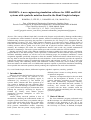
Proceedings of the 8th WSEAS Int. Conference on SOFTWARE ENGINEERING, PARALLEL and DISTRIBUTED SYSTEMS
BONDIN: A new engineering simulation software for ODE and DAE
systems with symbolic notation based in the Bond Graph technique
ROMERO, G.; FÉLEZ, J.; CABANELLAS, J. M.; MAROTO, J.;
Dep. of Mechanical Engineering. Engineering Graphics Group.
Escuela Técnica Superior de Ingenieros Industriales. Universidad Politécnica de Madrid
C\José Gutiérrez Abascal Nº 2. 28006 Madrid. Spain
Tel +34 91 336 31 15 FAX: +34 915 618 618
e-mail: [gregorio.romero, jesus.felez, josemaria.cabanellas, joaquin.maroto]@upm.es
Abstract: The concept of Bond Graph (BG), introduced by Paynter and perfected by Karnopp and Rosenberg
[1] contributed a unified method to describe dynamic models of multidisciplinary systems since they can be
modelled using elements possessing the properties of generation (Se, Sf), storage (I, C), dissipation (R) and
transformation of energy (TF, GY). These elements interrelate in a conservative energy field by means of
bonds that indicate the energy transfer and bonds (0, 1), which symbolise the system’s dynamic behaviour. The
resulting structure offers a global view of the system and its physical structure. Moreover, after obtaining
causality, this technique also offers the computational structure and reveals any possible mathematical
problems in simulating it. The entire system remains open and accessible unlike the classical methods.
Starting out from a study of the different simulation programs available, this paper presents a simulation
program based on the BG technique, which represents a considerable advance towards improving current
automatic modelling methods. As will be seen in the following pages, the technique contributes a causal
assignation algorithm specifically designed to allow the modeller maximum freedom without their having to
take any kind of decision that might affect the end calculation. It also automatically provides the optimised,
reduced state equations required to symbolically analyse linear and non-linear systems. To do so, it solves the
problems arising when simulating models with differential causality without any need to modify the graph
charts and reduces the model to the set of differential equations required to perform the simulation, eliminating
where possible the restriction equations, thereby reducing the computation time used in the simulation.
Key words: Bond Graph, software, differential equations, algebraic equations, causality, symbolic.
difficulty when it comes to solving them by means
of numerical integration.
Therefore, an important objective that was dealt
with in the development of Bondin © was to
generate alternative procedures to existing ones,
that would automatically implement causality,
analyse the BG and obtain the break variables, if
necessary, and consider the DAE equations
associated with the break variables inside the
differential equations and finally solve the resulting
system of equations.
1 Introduction
Efforts to automate the BG method in recent years
have focused on solving the problem of the
dependent co-ordinates that frequently appear in
mechanical [2], electrical [3] and thermal [4]
systems. Some solutions that have appeared up to
now consist in handling the state equations either
manually [2] or with the help of symbolic calculators
[5]. Other solutions add stiff type elements that allow
relaxing the system by increasing its degrees of
freedom [6]. Finally, some authors propose
introducing Lagrange multipliers to solve the
problem [2] [7].
Another mainly unsolved problem is that of
automatically obtaining the mathematical model of
complex systems where there is any number and type
of zero order causal paths (ZCP); that is, paths along
which there are no integration operations. These
ZCPs generate mathematical models comprising
DAE systems that can present varying degrees of
ISSN: 1790-5117
2 State-of-the-art
The first simulation program performed using
the BG technique was called ENPORT [8] and was
developed at the beginning of the 70s at the
University of Michigan. At the end of this decade
the University of Twente, in Holland, developed
90
ISBN: 978-960-474-052-9
Proceedings of the 8th WSEAS Int. Conference on SOFTWARE ENGINEERING, PARALLEL and DISTRIBUTED SYSTEMS
another BG-based tool called THTSIM in Europe and
TUTSIM in the United States.
Later, at the beginning of the 90s, the same
research group that had developed THTSIMTUTSIM produced CAMAS, based on the SIDOPS
simulation language that would eventually evolve
into 20-SIM. Also at the beginning of the 90s,
Madrid Technical University, the University of
California and the University of Michigan developed
other similar software (BONDYN, CAMP-G and
CAMBAS), the two latter with the purpose of
converting a BG into a series of data that would be
valid for digital simulation languages (DSL) and for
working with machines running the SUN operating
system respectively. Halfway through the 90s,
Research Park Ideon, Sweden, developed DYMOLA,
a general purpose modelling and simulation program
developed in the language oriented towards
MODELICA objects, which offered the possibility of
representation using BG. Also halfway through the
90s, the University of Glasgow generated software
called MTT. At the end of the 90s a modelling
workbench developed in partnership with EDF
(Electricité de France) generated MS1, which
performed a symbolic manipulation of the equations
in the model by means of causal analysis, generating
the code required to run the simulation. Also in the
same period the Indian Institute of Technology
carried out SYMBOLS, which permitted hierarchic
modelling using objects and systems control.
Apart from the tools specified above, there are
other less widespread applications (ARCHER,
PASION-32, BONDLAB, HYBRSIM).
In sum, it may be said that the most advanced
applications usually generate instructions in a
particular language so that once complied it can be
run and simulated. Some of the other computer
applications can only be used with linear systems and
constant parameters. In other cases, the user is
required to make decisions that usually lead to
unequal results. Finally, should there be any, the
equations obtained, either symbolically or
numerically, are only for the user to understand the
simulation model and not to be worked with in depth.
Therefore, taking the existing software as a basis,
in 2002 work was begun on a tool that would be
capable of correctly obtaining the causality of the
models so that the modeller would have maximum
freedom and the tool then automatically provide the
optimised reduced state equations required to analyse
linear and non-linear systems symbolically and
finally go on to simulate ODE and DAE systems.
Bondin © has been used in numerous papers [10][15] and pieces of research work undertaken by the
authors since then and it has now been decided to
propagate it among the scientific community.
ISSN: 1790-5117
3 Main characteristics
This software incorporates algorithms for causal
analysis and for reducing DAE systems of
equations to ODE, whenever possible, that have
been developed to that end. Thus, the main features
are:
• Bond Graph model simulation and variable
parameters that are user- programmable, either
under pseudo-programming or by calling on
external dynamic libraries without the need to
do any compilation whatsoever.
• The different elements are parametrically and
symbolically defined.
• Subset libraries are east to create.
• A model can be given unlimited hierarchical
structuring using subsets.
• Automatic generation of causality.
• The equations resulting from the model can be
obtained symbolically and legibly.
• Obtaining the minimum set of equations by
reducing the number of constraint equations
and using symbolic operations automatically.
• Numerical resolution of the model and graphic
output.
Throughout the following sections a brief
description will be made of the visible part and of
the different algorithms developed that have been
used.
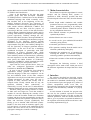
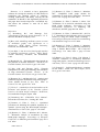
4 Interface
The software described here basically consists
of a menu bar, a tool bar and a work window where
the model to be simulated is defined (fig. 1), either
by the notation of ports and graphs or by means of
subsets encapsulated under icons that are
hierarchically structured in the program installation
directory and automatically reflected in a pop-up
window.
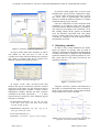
As each element is inserted, the program asks
the user for the symbolic expression associated
with its definition in order to be able to relate the
different parameters with one another and thus be
able to go on to produce an optimal formulation of
the equations associated with the model once it has
been fully implemented (fig 2).
91
ISBN: 978-960-474-052-9
Proceedings of the 8th WSEAS Int. Conference on SOFTWARE ENGINEERING, PARALLEL and DISTRIBUTED SYSTEMS
So that the results graphs show a correct result
(displacement, speed, pressure, temperature, angle,
…) and the values associated with each port have
the correct units of measurement, the physical
domain to which the different elements of a model
simulation belong can be selected.
Once the composition of a BG model has been
completed, as to both the form and the values
associated with the different elements, everything is
now ready for proceeding to the simulation. To do
this, initially almost all the options are disabled,
since the functions associated with each option
require a certain order. Due to this, as one function
or another is completed, new menu options will be
automatically activated.
5 Obtaining causality
In order to carry out the simulation of a model,
firstly an analysis of causality must be made to
indirectly determine the dependent and independent
variables, the number of algebraic and differential
equations and detect any possible problems. It is for
this reason that the only option activated at the
beginning is this one.
Figure 1: Schematic capabilities of Bondin ©.
In respect of the name of the elements, as will be
seen further on, this will serve to refer to the
variables associated with the different ports when the
user needs to program and also to interpret the
different equations and graphs produced.
Figure 2: Parameters dialogue box.
Figure 3: ´Calculation´ menu.
In respect of the value associated with each
element, this may be a numerical, symbolic or mixed
expression. In the latter case the expression may be
dependent on the generic variable ‘t’ (time) or on the
independent variables. Besides the basic operators
contained in the whole expression (+, -, *, /), these
expressions may contain any of the following typical
functions or constants:
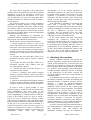
Using the ‘Causality’ option a causal analysis of
the model is performed and the result is shown by
means of the causality lines on the graphs and their
being assigned one colour or another.
• Trigonometric functions: sin, cos, tan, cot, asin,
acos, atan, ascot, sinh, cosh, tanh, coth, arsinh,
arcosh, artanh, arcoth.
• Mathematical functions: sqr, sqrt, exp, lg, ln,
abs, sgn, round, fac, rand.
• Universal constants: pi, e.
• Operators: ! (factorial), ^ (power), % (percentage).
Figure 4: Electrical operation of a lathe by using PI type
regulators with solved causality in Bondin ©.
ISSN: 1790-5117
92
ISBN: 978-960-474-052-9
Proceedings of the 8th WSEAS Int. Conference on SOFTWARE ENGINEERING, PARALLEL and DISTRIBUTED SYSTEMS
automatically one of the integral causalities to
differential causalities, the study can be continued.
If another similar conflict is again found, the same
operation is performed on successive integral
causalities. By this procedure, there should only
remain as many ports with integral causality as
there are degrees of freedom.
If the algorithm is incapable of continuing and
enters into a recurring loop, the causality
assignation starts again and checks that each time a
causality is imposed if a conflict is created or not. If
the case is affirmative, go back and clean
everything that has happened since this latest
imposition of causality and carry on with the
following element or intermediate bond.
If the causal analysis has been successfully
completed, the ‘Parameters’ option will be
activated in the menu below the ‘Causality’ menu,
from which, strictly speaking, the simulation will
be performed after assigning numerical values or
programming on the user-inserted parameters. To
do this, the program automatically analyses each
and every one of the written expressions and
deduces the names of the different parameters.
The colour blue is assigned to the graphs where
causality has been obtained from other pre-calculated
causalities or due to the imposition of integral or
differential causalities on the different I or C ports
(fig. 4) while pink is reserved for the graphs where
causality needed to be imposed in order to obtain a
correct analysis.
The program consists of two causal assignation
algorithms. It initially attempts to assign causality
using the first algorithm, but if this cannot be done
successfully, it does so with the second one. If this is
the case a message appears to inform of this with the
only purpose of stating which of the two algorithms
has been satisfactorily used.
Karnopp and Rosemberg [1] introduced the
sequential causality assignation procedure (SCAP),
this being the conventional procedure to use.
This procedure consists of the following steps:
1.- Assign appropriate causality to one of the
sources and extend across the other nodes. Repeat
until all the sources have been taken account of.
2.- Choose any I or K element and assign integral
causality. Extend it across the other nodes. Repeat
until all the I and K ports have been taken into
account.
3.a.- Examine the state of the BG: If there is an
incomplete causality, with no conflicts, continue
in step 4.
3.b.- Examine the state of the BG: If there is an
incomplete causality, with conflicts, stop and
correct the model by the user.
3.c.- Examine the state of the BG: If there is a
complete causality, finalise.
4.- Choose a resistance port without assigned
causality, assign an arbitrary causality and extend
it. Repeat until all the resistances have been taken
into account.
5.- Choose an intermediate bond without assigned
causality, assign an arbitrary causality and extend
it. Repeat until all the bonds have been completed.
6 Obtaining the equations
Having calculated causality and inserted the
different parameters requested, the following two
options of the submenu (fig. 3) become active and
from here we proceed to calculate the differential
and/or algebraic-differential equations of the model
in a symbolic form depending on the independent
variables and those inserted by the user. According
to the compelexity of the model, reducing the
system of equations can involve a large amount of
computation time.
At ICBGM’05 (New Orleans, USA) [9] two of
the authors presented a procedure for obtaining the
minimum number of equations necessary and for
reducing a system of algebraic-differential
equations to a purely differential one within a
simulation model carried out with a bond graph,
and based only on causal assignation. The method
employs a series of basic rules for assigning
causality correctly in order to avoid any type of
incompatibility. Subsequently, depending on the
different types of causal paths and algebraic loops
coexisting, through a succession of algebraic
operations carried out on matrices, the method is
capable of obtaining a system of reduced equations,
all of which is done by using symbolic notation.
As can be seen from the paper mentioned above
[9], any model can be condensed into a general one
that contemplates ports with integral and
differential causality, and type “R” elements or
In order to study a greater number of cases
without having to change the BG model structure,
some modifications have been made to this
procedure. These are in point 3.b, where the option of
causal compatibility or conflicts has been considered.
Firstly, if the conflict occurs in a node to which a
type I or C port is attached, the causality of these
ports changes automatically. They will initially have
integral causality and then become differential. When
all the type I or C ports have been concluded, if a
conflict is produced in a node to which no type I or C
element is attached, the next step is to eliminate all
information referring to causality in resistances and
intermediate
bonds.
Then,
after
changing
ISSN: 1790-5117
93
ISBN: 978-960-474-052-9
Proceedings of the 8th WSEAS Int. Conference on SOFTWARE ENGINEERING, PARALLEL and DISTRIBUTED SYSTEMS
⎡
⎛
⎡ Se_Ri ⎤ ⎤ ⎞
⎜
⎢
⎢
⎥⎥⎟
Se_I ⎤ d ⎜⎜ ⎡ 1 ⎤ ⎢⎢
⎡Pm_i( t )⎤ + [ F ] ⎡Se_i( t )⎤ + [ G ] ⎢⎢ Sf_Ri ⎥⎥ ⎥⎥ ⎟⎟
(-1) ⎡⎢⎢
[
E
]
⎥⎥ = ⎜ ⎢⎢
⎢
⎥
⎢
⎥
⎢
⎢
⎥⎥⎟
⎥
⎥
⎢
⎥
⎢
⎥
⎜
⎢
⎢
⎥⎥⎟
[
J
]
d
t
⎦⎢
⎣Sf_C ⎦
⎣XK_i( t )⎦
⎣ Sf_i( t )⎦
⎜⎣
⎢Se_gr_i⎥ ⎥ ⎟
⎜⎜
⎢⎢
⎢⎢
⎥⎥ ⎥⎥ ⎟⎟
⎝
⎣
⎣ Sf_gr_i ⎦ ⎦ ⎠
intermediate bonds where it has been necessary to
assign arbitrary causality. The way to proceed is
exactly the same in the singular cases but, obviously
the complexity will be somewhat greater, as there
will now be three interrelated systems instead of two.
In these cases, once the three systems of equations
have been formed:
⎡ Se_Ri ⎤
⎡ d Pm_i( t )⎤
⎥
⎢
⎥
⎢
⎢ Sf_Ri ⎥
⎥
⎢dt
Se_i( t )⎤
⎥ + [ D ] ⎡⎢ Se_I ⎤⎥
⎢
⎥ = [ A ] ⎡⎢Pm_i( t )⎤⎥ + [ B ] ⎡⎢
⎢
[
C
]
+
⎥
⎥
⎢
⎥
⎢d
⎢Sf_C ⎥
⎥
⎢
⎥
⎢
⎥
⎢
⎥
⎢
⎦
⎣
⎣ Sf_i( t )⎦
⎣XK_i( t )⎦
⎢Se_gr_i⎥
⎢ Xk_i( t ) ⎥
⎥⎥
⎢⎢
⎥
⎢ dt
⎦
⎣
⎣ Sf_gr_i ⎦
⎡ Se_Ri ⎤
⎡
⎡ Se_Ri ⎤ ⎤
⎢
⎢
⎥
⎢
⎥⎥
⎢ Sf_Ri ⎥
⎢
⎢ Sf_Ri ⎥ ⎥
Pm_i( t )⎤
Se_i( t )⎤
⎡
⎡
⎢
⎢
⎥
⎥⎥
[ Sgn ] ⎢
⎥⎥ + [ M ] ⎢⎢
⎥⎥ + [ N ] ⎢⎢
⎥ = [ P ] ⎢ [ L ] ⎢⎢
⎥⎥
⎢Se_gr_i ⎥
⎢
⎢Se_gr_i ⎥ ⎥
⎣XK_i( t )⎦
⎣ Sf_i( t ) ⎦
⎢
⎢
⎥
⎢
⎥⎥
⎢⎢
⎢⎢
⎥⎥
⎢⎢
⎥⎥ ⎥⎥
⎣ Sf_gr_i ⎦
⎣
⎣ Sf_gr_i ⎦ ⎦
[ A1 ] =
To reduce the systems (1) to (3), which are
composed by differential and algebraic equations,
we can reformulate the systems and a final system
of differential equations can be obtained:
⎡ d Se_i( t )⎤
⎡ d Pm_i( t )⎤
⎢
⎥
⎢
⎥
⎢dt
⎥
⎢dt
⎥
Pm_i( t )⎤
⎡Se_i( t )⎤
⎢
⎥
⎢
⎥ = [ A1 ] ⎡⎢
[
B2
]
[
B1
]
+
+
⎥⎥
⎥⎥
⎢⎢
⎢
⎥
⎢d
⎥
⎢
Sf_i( t ) ⎦
XK_i( t )⎦
⎢d
⎥
⎢
⎥
⎣
⎣
⎢ Sf_i( t ) ⎥
⎢ Xk_i( t ) ⎥
⎢dt
⎥
⎢ dt
⎥
⎣
⎦
⎣
⎦
(1)
[P] [ L ]
[P] [ L ]
[P] [ L ]
⎤ − [D] ⎡⎛ d ⎛ [ E ] ⎞⎞ + ⎛ d ⎛ [G ] ⎞⎞ ⎡
⎤⎞⎤
⎤ + ⎡ [G ] ⎤ ⎛ d ⎡
[ A ] + [ C ] ⎡⎢⎢
⎢⎢ ⎜⎜ ⎜⎜
⎥⎥
⎥⎥ ⎟⎟ ⎥⎥
⎥⎥ ⎢⎢
⎥⎥ ⎜⎜ ⎢⎢
⎟⎟ ⎟⎟ ⎜⎜ ⎜⎜
⎟⎟ ⎟⎟ ⎢⎢
⎣ [Sgn] − [ P ] [ N ] ⎦
⎣ ⎝ dt ⎝ [ J ] ⎠ ⎠ ⎝ dt ⎝ [ J ] ⎠ ⎠ ⎣ [Sgn] − [ P ] [ N ] ⎦ ⎣ [ J ] ⎦ ⎝ dt ⎣ [Sgn] − [ P ] [ N ] ⎦ ⎠ ⎦
[
P
]
[
L
]
⎡ [ E ] + [G ] ⎡
⎤⎤
⎢
⎢⎢
⎥⎥ ⎥
⎢
⎣ [Sgn] − [ P ] [ N ] ⎦ ⎥⎥
[ I ] + [ D ] ⎢⎢
⎥
J
[
]
⎣
⎦
[ P ] [M ]
⎤+
⎛ [ F ] ⎞ ⎞ + ⎛ d ⎛ [ G ] ⎞ ⎞ ⎡⎢
⎥
⎜⎜
⎟⎟ ⎜ ⎜
⎟⎟
⎝ [ J ] ⎟⎠ ⎟⎠ ⎜⎝ dt ⎜⎝ [ J ] ⎟⎠ ⎟⎠ ⎢⎣ [Sgn ] − [ P ] [ N ] ⎥⎦
[P ] [ L ]
⎡⎢ [ E ] + [ G ] ⎡⎢
⎤⎤
⎢ [Sgn ] − [ P ] [ N ] ⎥⎥ ⎥⎥
⎢
⎣
⎦⎥
⎢
[I] + [D] ⎢
⎥
[J]
⎣
⎦
[D] ⎤ ⎡
[ P ] [M]
⎡
⎤⎤
- ⎡⎢⎢
⎥⎥ ⎥⎥
⎥⎥ ⎢⎢ [ F ] + [ G ] ⎢⎢
⎣ [Sgn] − [ P ] [ N ] ⎦ ⎦
⎣ [J] ⎦ ⎣
[
P
]
[
L
]
⎤⎤
⎡ [ E ] + [G ] ⎡
⎢
⎢⎢
⎥⎥ ⎥
⎢
⎣ [Sgn] − [ P ] [ N ] ⎦ ⎥⎥
[ I ] + [ D ] ⎢⎢
⎥
[
J
]
⎦
⎣
(7)
[ P ] [M ]
⎡
⎤⎞⎤
⎢⎢
⎥⎥ ⎟⎟ ⎥⎥
⎣ [Sgn ] − [ P ] [ N ] ⎦ ⎠ ⎦
(6)
7 Calling the variables
To define the value associated with the different
elements, it has been seen that those values can be
numerical or symbolic expressions. In the latter
case, the parameters can be constant, conditioned
variables inserted by the user or the dependent and
independent variables associated with the different
ports.
In order to be able to call a dependent or
independent variable, either when writing the
expression associated with a specific parameter or
when writing a certain condition, these variables
must take the form shown below.
Should the variable correspond to an
'Inertance' type port (named 'I_n'), that variable
must be the speed 'V' of that port (in translational
mechanics) and its integral, and 'X' the movement
(also in translational mechanics), which means it
will be called by placing the letter 'V' or 'X' before
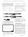
===================== NON-REDUCED EQUATIONS (DAE) =====================
----------------------------------------- Algebraic-differential equations ----------------------------------------d/dt[VI_1]=-1/m1*R*VI_1+1/m1*K*XK_1-1/m1*m2*g+1/m1*R*Vo-g - 1/m1*m2*d/dt[VI_2]
d/dt[XK_1]=-VI_1+Vo
VI_2=VI_1
======================= REDUCED EQUATIONS (ODE) =======================
------------------------------ Differential equations -----------------------------d/dt[VI_1]=(-1/(m2+m1)*R)*VI_1+(1/(m2+m1)*K)*XK_1+(1/(m2+m1))*
*(-m2*g) + (1/(m2+m1)*R)*(Vo)+(1/(m2+m1))*(-m1*g)
d/dt[XK_1]=(-1)*VI_1+(1)*(Vo)
equations.txt
d/dt[VI_2]= d/dt[VI_1]
Figure 5: File with equations obtained from a model
composed by two inertances with a rigid union.
As soon as the calculation of the ODE/DAE
expressions has been concluded, these can be viewed
ISSN: 1790-5117
⎡ [ G ] ⎤ ⎛⎜ d
⎢⎢
⎥
⎣ [ J ] ⎥⎦ ⎜⎝ dt
(5)
in a form that is user-readable (fig. 5) and they can
be numerically simulated.
When a pre-calculation of the DAE and ODE
system equations has been made, they can then be
simulated independently in order to reach
conclusions and undertake time studies.
To obtain the equations defining a model totally
automatically that are user-transparent Maple © must
be used. This should be installed in the computer to
carry out symbolic operations such as matrix
manipulation, deriving and simplifying expressions.
---------------------------- Algebraic equations ---------------------------VI_2=VI_1
(4)
The equations (4) can be generated
automatically simply by operating and deriving the
different matrices as follows:
(2)
[ P ] [M]
⎤ − [D] ⎡⎛ d
[ B ] + [ C ] ⎡⎢⎢
⎢⎢ ⎜⎜
⎥
[Sgn ] − [ P ] [ N ] ⎥⎦
⎣ ⎝ dt
⎣
[ B1 ] =
[ B2 ] =
(3)
94
ISBN: 978-960-474-052-9
Proceedings of the 8th WSEAS Int. Conference on SOFTWARE ENGINEERING, PARALLEL and DISTRIBUTED SYSTEMS
the name of the port (I_n); in addition the character
reserved '_' will need to be placed before and after.
if ((abs(_VI1_-_VI2_)>0) and (abs(_VI1_-_VI2_)<=5))
{
750
};
'_' + 'V' or 'X' + name_port_Inertance + '_'
if ((abs(_VI1_-_VI2_)>5) and (abs(_VI1_-_VI2_)<=10))
{
1000
};
Thus, '_VI_n_' would be used to indicate the
speed or the independent variable associated with the
inertance 'I_n' and '_XI_n_' to indicate its movement
or the integral of the previous independent variable.
If dealing with 'Compliance' type ports (named
'C_n'), the variable to be taken into account is its
movement 'X' (in translational mechanics), its
integral having no physical sense. Therefore, in this
type of port, the letter 'X' should be placed before the
name of the element in question (C_n) and the
character '_' placed before and after.
if (abs(_VI1_-_VI2_)>10)
{
1500
};
Figure 6: Pseudo-code of a variable parameter.
Calling a function from an external *.dll-type
library will be done when the code is too complex
to do it using simple conditions and must be
compiled as a dynamic library (DLL).
To make the call the reserved word 'DLL' must
first appear to indicate that an external library
needs to be loaded, and then the name of the '*.dll'
dynamic library that it is wished to load and the
name of the function to be called. Finally, the
different variables must be indicated in the
appropriate order, whose numerical values are
required to be passed to the function in question, it
not being necessary to do it with the time variable
't' since this is an internal variable. The different
names and variables mentioned above must be
separated by the reserved character '$'.
'_' + 'X' + name_port_Compliance + '_'
Thus, we will get '_XC_n_' to indicate the
movement made by the spring 'C_n' or the
independent variable associated with that element.
8 Programming: scripts and dlls
Sometimes, when it is wished to perform a
simulation with greater realism and therefore greater
complexity, it is not sufficient to insert constant
parameters or variables that are governed by a
particular expression. What must be done is to
program a series of conditions that will make these
variables vary in one way or another. While on some
occasions it is sufficient to write some simple
conditions, on others it is not and functions belonging
to more complex external libraries need to be called
on.
To this end, two modules have been designed
through which conditions can be inserted in one way
or another.
Should it be wished to insert conditions directly,
each of them must begin with the reserved word ‘if’
and immediately after in brackets the requirement
wished to be met must be written. Then, in brace
brackets the numerical value must be placed or the
expression linked to the condition. Finally, in order
to indicate that writing the condition has concluded, a
semi-colon must be put in place. Should there be
several requirements in a single condition, each of
these must be in brackets and separated by the
reserved word 'and'.
Thus, in order to program a variable damper so
that depending on the difference of speed between its
ends (inertances ‘I1’ and ‘I2’), the damper is softer or
harder, it would suffice to write it as shown in figure
6.
ISSN: 1790-5117
DLL$library$function$parameter1$..$ parameterN$
Therefore, if it is wished to define the value of
the damper in the previous example by calling the
'hardness' function corresponding to the library
'characteristics.dll', by passing on to it as
parameters the speed of the inertances situated at
the ends 'I1' and ‘I2’ (‘_VI1_’ and‘_VI2_’), it will
need to be written in the following form:
DLL$characteristics$hardness$_VI1_$_VI2_$
9 Creating and handling subsets
When it is required to repeatedly create models
containing several similar structures, as for
example, a hydraulic circuit [13] or a mechanism
comprising several bars [15], this task can be
simplified by saving these structures individually
and then inserting them where they are needed, as
if they were new elements.
To create a subset, all that needs to be done is to
design the model in question and leave a series of
incomplete nodes through which the remaining
elements of the end model will be connected at a
future time.
95
ISBN: 978-960-474-052-9
Proceedings of the 8th WSEAS Int. Conference on SOFTWARE ENGINEERING, PARALLEL and DISTRIBUTED SYSTEMS
Figure 7: Front-loader mechanism by using subsets in Bondin ©.
As can be seen, the speed with which a complex
model can be prepared from previously saved and
configured models makes this a very useful tool for
generating large models. On the other hand, if it is
compared with its original model, its simplicity
makes it much easier to understand. Finally, given
the importance of the issue, particular emphasis has
been placed on the fact that a subset can be inserted
into another as many times as required, with no limits
of levels.
As we have commented throughout, the systems
generated can be of type ODE or DAE. While the
former can be solved with a large quantity of
algorithms, the latter requires specific numerical
methods to solve it, for which reason Dassl [16]
has been chosen for its robustness and rapid
convergence.
11 Conclusion
The problems involved in any model made by a
Bond-Graph are directly related to causality and are
greater the more complex the calculation. Many of
the options put forward in other works attempt to
simplify the calculation of causality and oblige the
user to carry out changes or simplifications to the
original model. This means that since it is the
modeller that makes the decisions, in many cases
the results vary or the simulation is simply not
carried out to completion.
On the other hand, the difficulty of numerically
solving a system of equations depends on the type
of system (ODE or DAE), and on the number of
equations, that is to say, the number of variables
and on the integration pass that is conditioned by
the appearance of certain elements.
Finally, every calculation that is made
symbolically instead of numerically allows a
clearer interpretation to be made together with a
global view of each and every parameter in the
model.
10 Obtaining the results
When a simulation has been successfully
completed, the results can be shown in graphic form
using a dialogue box that allows choosing the
variables to be displayed, either individually or as a
set, and lets certain areas be zoomed in on.
Angle of ‘J1’ (rad) _ Time (s)
Angle of ‘J2’ (rad) _ Time (s)
Figure 8: Superimposed graphs obtained.
ISSN: 1790-5117
96
ISBN: 978-960-474-052-9
Proceedings of the 8th WSEAS Int. Conference on SOFTWARE ENGINEERING, PARALLEL and DISTRIBUTED SYSTEMS
[11] Romero, G., Félez, J., Maroto, J., Martínez,
M.L. “Simplified bond graph models for
simulations of earth moving machines“. Simulation
Series. Vol. 39. pags 139 a 147. 2007.
However, it is essential to have appropriate
software for solving the causality of a BG model, for
simplifying the resulting system of equations,
working symbolically and finally carrying out the
simulation. In Bondin © the algorithms proposed in
this paper have been developed in a condensed way
that allows the software to meet all of these
conditions.
[12] Romero, G., Félez, J., Maroto., J., Mera, J. M.
“Simulation of an electrical substation using the
Bond Graph technique“. Proceedings of 10th
International Conference on Modelling and
Simulation, de IEEE, pags 584-589. 2008.
References
[1] Rosemberg, R.C. and Karnopp, D.C.
“Introduction to Physical System Dynamics”. N. Y.
McGraw-Hill Book Company. 1983.
[13] Romero, G., Félez, J., Martínez, M.L., del Vas,
J. J. “Simulation of the hydraulic circuit of a wheel
loader by using the Bond Graph technique “.
Proceedings of European Conference on Modelling
and Simulation. Pags 313 a 321. 2008.
[2] Bos, A.M. “Modelling mulibody systems in terms
of multibond graphs with application to a
motorcycle”. Ph.D. Thesis. Twente University,
Enschede, The Netherlands. 1986.
[14] Romero, G., Félez, J., Maroto., J., Martínez,
M.L. “Simulation of an Asynchronous Machine by
using a Pseudo Bond Graph“. AIP Conference
Proceedings. Vol. 1060, Issue 1, pags 137-146.
2008.
[3] van Dijk, J. “On the role of bond graph causality
in modelling mechatronic systems”. Ph.D. Thesis.
Twente University, Enschede, The Netherlands.
1994.
[15] Romero, G., Félez, J., Mera, J. M., Maroto, J.
“Efficient simulation of mechanism kinematics
using bond graphs“. Simulation Modelling Practice
and Theory. Vol. 17, Issue 1, pags 293-308. 2009.
[4] Breedveld, P.C. “Thermodynamic bond graphs an
the problem of thermal inertances”. Journal of the
Franklin Institute, Vol.314, No.2, pp.15-40. 1982.
[16] Petzold, L. “Differential/algebraic equations
are not ODE's”. SIAM J.Sci. Stat. Comput., Vol.3,
No.3, pp.367-384. 1982.
[5] Bos, A.M. and Tiernego, M.J.L. “Formula
manipulation in bond graph modeling and simulation
of large mechanical systems”. Journal of the
Franklin Institute. Vol.319, No.1/2, pp.51-65, 1985.
[6] Karnopp, D. C. and Margolis, D.L. “Analysis and
simulation of planar mechanisms using bond graphs”.
Trans. ASME Journal of Syst. Dyn., Meas. &
Control, Vol. 101, pp.187-191. 1979.
[7] Fé1ez, J. “A method for the unified análisis of the
kinematic and dynamic of the vehicular systems
based in the Bond Graph technique”. Ph.D.Tesis,
Universidad de Zaragoza, Spain. 1989.
[8] Rosenberg, R.C. “ENPORT-6 User's Manual”.
Rosencode Associates, Inc., Lansing, MI. 1985.
[9] Romero, G., Félez, J., Vera, C.; “Optimised
procedures for obtaining the symbolic equations of a
dynamic system using the Bond-Graph technique“.
Simulation Series.Vol.37,Nº1, pags 51 a 58. 2005.
[10] Romero, G., Félez, J., Martínez, M.L., Maroto,
J.; “Kinematic analysis of mechanism by using
Bond-graph language“. Proceedings of European
Conference on Modelling and Simulation. pags 155 a
165. 2006.
ISSN: 1790-5117
97
ISBN: 978-960-474-052-9