Download ThunderSTORM: a comprehensive ImageJ plugin for PALM and

Charles University in Prague
First Faculty of Medicine
Institute of Cellular Biology and Pathology
ThunderSTORM: a comprehensive ImageJ
plugin for PALM and STORM data analysis
and super-resolution imaging
User’s Guide
Version 1.1
Martin Ovesný, Pavel Křı́žek, Josef Borkovec, Zdeněk Švindrych, and Guy M. Hagen
Contents
1.
About ........................................................................................................................................ 2
1.1.
Installation .......................................................................................................................... 2
1.2.
Compatibility notes ............................................................................................................. 2
1.3.
Help with ImageJ ................................................................................................................ 2
1.4.
Help with ThunderSTORM................................................................................................. 2
1.5.
Initial settings of ImageJ ..................................................................................................... 2
1.6.
Updating ThunderSTORM.................................................................................................. 3
1.7.
Input / Output ..................................................................................................................... 3
1.8.
Building ThunderSTORM................................................................................................... 3
1.9.
Report a bug ....................................................................................................................... 3
2.
Processing 2D data ................................................................................................................... 4
3.
Processing 3D data (astigmatism method) ............................................................................... 8
4.
Post-processing modules......................................................................................................... 10
4.1.
Filter ................................................................................................................................. 10
4.2.
Remove duplicates ............................................................................................................ 11
4.3.
Merging ............................................................................................................................ 11
4.4.
Drift correction ................................................................................................................. 11
4.5.
Z-stage offset .................................................................................................................... 12
4.6.
Visualizing and exporting molecular localizations from a region of interest ....................... 12
5.
Analyzing super-resolution images with ImageJ ................................................................... 13
6.
Specifying a threshold for detection of molecules .................................................................. 14
7.
Generator of simulated data .................................................................................................. 16
8.
Performance evaluation ......................................................................................................... 16
9.
Monte Carlo simulations – an example using the ImageJ Macro Language ........................ 17
1
1.
About
1.1. Installation
ThunderSTORM is written in Java and is distributed under the terms of the GNU GPLv3 license as a
plugin for ImageJ. The official download site for the latest version of ImageJ is accessible at
http://rsbweb.nih.gov/ij/download.html. Note that ImageJ requires the Java Runtime Environment
(JRE) to be installed. If you do not have JRE installed, download a bundled version of ImageJ & JRE
for your platform. We recommend using the 64-bit version of Java for a 64-bit operating system.
To install the ThunderSTORM plugin for the first time, download the latest version from the website
https://code.google.com/p/thunder-storm/ and copy the Java Archive file (Thunder_STORM.jar) into
the plugins subfolder of your ImageJ installation. The location on a Windows system is, for example,
“C:\Program Files\ImageJ\plugins\Thunder_STORM.jar”.
To verify successful installation of ThunderSTORM, run ImageJ. There should be an item called
ThunderSTORM in the Plugins menu of ImageJ. If the item does not exist, make sure that the file name
Thunder_STORM.jar is correct as it has to contain the underscore “_” character.
1.2. Compatibility notes
·
·
·
ThunderSTORM has been tested on Windows XP (32b), Windows 7 (32b/64b), Debian and
Ubuntu Linux (32b/64b), and MacOS X 10.8.5.
ThunderSTORM is compatible with ImageJ based applications such as Fiji and μManager.
ThunderSTORM is compiled for Java 1.6 and is compatible with ImageJ 1.45s or later.
1.3. Help with ImageJ
The official ImageJ documentation is available at http://rsbweb.nih.gov/ij/docs/guide/user-guide.pdf.
1.4. Help with ThunderSTORM
To get help with using ThunderSTORM, please consult this User’s manual or the project Wiki page.
To get help related to a specific function, click on a blue icon with a question mark
next to
a particular control panel. A detailed description of algorithms used for the data analysis is also
available in the Supplementary Note ThunderSTORM: Methodology and Algorithms. All
documentation is accessible at https://code.google.com/p/thunder-storm/.
1.5. Initial settings of ImageJ
Since data acquired by Single Molecule Localization Microscopy (SMLM) are usually very large
(several GB) and processing the data is computationally demanding, we recommend setting the
number of processing threads equal to the number of available CPU cores. It is also crucial to set the
memory limit to the highest possible value, but at the same time to keep enough memory (~2 GB) for
the operating system.
For example, our setup uses a computer with an Intel i5 (4 cores) processor and 32 GB of RAM. We
set the number of processing threads to 4 and the memory limit to 30 GB. To decrease memory
consumption, load your data as a virtual stack (see ImageJ documentation).
To set the number of processing threads and the memory limit in ImageJ, select Edit → Options →
Memory & Threads.
2
1.6. Updating ThunderSTORM
ThunderSTORM has an integrated updater. From ImageJ, select Plugins → ThunderSTORM → Check
for updates... and select the version you want to upgrade (or downgrade) to, and click OK. If the
updater cannot be used for some reason, download the latest Thunder_STORM.jar file from the project
website, and copy it into the plugins subfolder of your ImageJ installation.
Please restart ImageJ before running the updated version of ThunderSTORM.
1.7. Input / Output
·
·
Images – all image formats supported by ImageJ and its plugins.
Molecular localizations and ground truth data – CSV, XSL, XML, YAML, JSON, and Tagged
Spot File (TSF) format.
1.8. Building ThunderSTORM
To make any changes or upgrades to the code on your own, and to build ThunderSTORM, clone the
Git repository by running the “git clone https://code.google.com/p/thunder-storm/”
command from the Git console. The repository contains a NetBeans 7.4 project which can be
compiled in the NetBeans IDE or from a console using the Ant utility.
In order to run ThunderSTORM directly from NetBeans, right-click on the Thunder_STORM project
and select Properties. Then select Run and type the ImageJ path into the Working directory text
field, for example, “C:\Program Files\ImageJ”. Note that running ThunderSTORM directly from
NetBeans will start ImageJ version 1.45s.
1.9. Report a bug
Prior to submitting a bug report, please upgrade to the latest version of ThunderSTORM and see if the
error still occurs.
If you receive an exception that ImageJ ran out of memory, try to increase the memory limit or to load
the SMLM data as a virtual stack (see ImageJ documentation).
In the case of a malfunction, please let us know by using the Google Code issue tracking system at the
project website: https://code.google.com/p/thunder-storm/issues/list. Please specify the malfunction,
and describe the procedure to reproduce the error. If an exception occurs, copy the stacktrace into the
description box and specify your platform, i.e., your versions of Java, ImageJ, ThunderSTORM, and
operating system.
3
2.
Processing 2D data
This is an example of the workflow for processing 2D SMLM data in ThunderSTORM. Note that
processing data with more channels should be done for each channel separately.
An example of (a fragment of) one of our real datasets is provided on the project website. More
datasets, both artificial and real, can be found on the Single-Molecule Localization Microscopy
Challenge website at http://bigwww.epfl.ch/smlm/.
Step 1 – Loading the data
Small datasets: Drag and drop the data file from the file explorer to ImageJ, or select File → Open
in ImageJ, browse to the data file and press Open. This will load the entire image stack into memory.
Large datasets: For datasets larger than the memory allocated to ImageJ, select File → Import →
TIFF Virtual Stack, browse to the file and press Open. This loads just a TIFF header and the
currently displayed frame into memory.
Sequence of images: If the dataset is not a single file but a sequence of files (all images have to be in
the same folder), select File → Import → Image Sequence, browse to the first image of the
sequence and press Open. The image sequence can also be opened with the Bio-Formats Importer
plugin, which is available at http://www.openmicroscopy.org/site/products/bio-formats. Please be sure
to use the latest version of Bio-Formats. For large datasets, use the Virtual stack option.
Step 2 – Camera settings
Set the camera pixel size in the sample plane, conversion factor between photons and digital units,
base level offset of the camera digitizer, and EM gain of the camera. This is important for fitting
methods and for estimation of localization accuracy, as these methods work with photon counts.
Plugins → ThunderSTORM → Camera setup
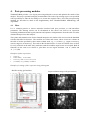
Step 3 – Processing the data
After opening the data, select Plugins → ThunderSTORM → Run analysis. There is a good deal of
freedom for experienced users to set the processing parameters. However, the default options provide
very good results on various datasets we have tried. Press OK to start the processing. An instant
preview of the results achieved so far during the data analysis is shown. The table with results appears
after the data analysis is finished.
Note that processing can be limited to an arbitrarily-shaped, user-specified region of interest in the
input images. This can greatly speed up the processing in large data sets. The processing can be
stopped at any point by pressing Escape on the keyboard.
Details about the algorithms used are accessible by clicking the particular help button, or in the
Supplementary Note ThunderSTORM: Methodology and Algorithms.
4
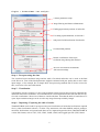
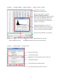
Plugins → ThunderSTORM → Run analysis
Camera parameters setup.
Image filtering and feature enhancement.
Finding approximate position of molecules.
For setting up the threshold, see Section 6.
Sub-pixel 2D/3D localization of molecules.
Crowded-field problem.
Instant visualization of the superresolution image during data analysis.
Preview of molecular localizations
with current settings.
Step 4 – Post-processing the data
The visualized super-resolution image and the table of localized molecules can be used as the final
result. However, some of the fitted parameters might be estimated with poor quality due to noise in the
input images, or for example, due to sample drift. Post-processing methods can be used to correct for
this, see Section 4 for more information.
Step 5 – Visualization
Visualization involves creation of a new, high resolution image based on the previously obtained subdiffraction molecular coordinates. Several methods have been implemented for both 2D and slice-byslice 3D visualization. Choose one of them to visualize the data. Note that the table of results has to be
open. Super-resolution images can be saved in any image format provided by ImageJ.
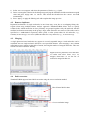
Step 6 – Importing / Exporting the table of results
ThunderSTORM can be used for post-processing and visualization of molecular localizations acquired
also by other localization software. To allow easy interaction with other SMLM analysis packages,
molecular localizations and ground truth data can be imported/exported to/from ThunderSTORM in
various file formats, such as: CSV, XSL, XML, YAML, JSON, and Tagged Spot File (TSF) format.
5
Plugins → ThunderSTORM → Import/Export → Show results table
Left click to sort values.
Right click to change units.
Results of the analysis: localized
molecules and their parameters.
Select rows and right click on the selection
to show the corresponding molecules in
the overlay layer of the raw data, or to
remove localizations in the selection by
Filter, see Section 4.
Plotting the histogram of values for
a particular variable can be used, e.g., to
remove molecules with poor localization
accuracy, see Section 4 for an example.
Post-processing methods, see Section 4.
Import/export of the results.
Camera parameters setup.
Visualization method for preview and final image.
Plugins → ThunderSTORM → Visualization
Defines camera ROI.
Visualization method.
Magnification with respect to the raw image size.
Visualization options.
Create final super-resolution image.
Use selected options for the live preview.
6
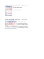
Plugins → ThunderSTORM → Import/Export → Export results
File name and data format.
Export data processing
protocol in YAML format.
Measurements for export.
Plugins → ThunderSTORM → Import/Export → Import results
File name and data format.
Allows to concatenate several
files with results into one table.
Show imported localizations as
an overlay in the image sequence.
7
3.
Processing 3D data (astigmatism method)
This is an example of the workflow for processing 3D SMLM data in ThunderSTORM in which the
axial molecular position is estimated from astigmatism introduced by a cylindrical lens. The procedure
is basically the same as in the case of processing 2D data. The only difference is that calibration of the
system needs to be performed prior to processing the data in order to estimate the axial positions. An
example of (a fragment of) one of our real 3D datasets is provided on the project website.
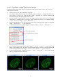
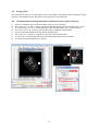
Step 1 – Calibration of the system
Load the calibration data and select Plugins → ThunderSTORM → 3D calibration → Cylindrical
lens calibration. The default settings for processing the data should be fine to use. Specify the
Z stage step (10 nm in our example dataset) and a location where the result of the calibration will
be saved. Then click OK to run the calibration. All necessary information for 3D fitting is saved in the
YAML file format.
Note that calibration can be limited to a user-specified region of interest in the input images.
Parameters of the fitted calibration curves and the
angle of the astigmatic lens with respect to the camera.
Calibration z-stack, where beads used for calibration
are marked with red circles and slice-by-slice subpixel localizations are marked with blue crosses.
Fitted calibration curves.
Step 2 – Processing the data
Load the image sequence acquired with the cylindrical lens and select Plugins → ThunderSTORM →
Run analysis. In the panel Sub-pixel localization of molecules, select PSF: Elliptical
Gaussian (3D astigmatism) and specify the path to the Calibration file generated in Step 1.
Click OK to run the analysis.
Step 3 – Visualization
Make sure that the 3D option is enabled in the visualization dialog to get 3D super-resolution images,
otherwise only a 2D image will be visualized. Specify the Z range to set the axial range and the step
between slices. Enable the Colorize z-stack option to get a color-coded z-position (implemented
as an ImageJ hyper-stack of channels with different lookup tables). Then Click OK.
8
Step 4 – Visualizing a rotating 3D projection (optional)
A rotating 3D projection of the data can be generated using ImageJ feature such as 3D Project ...
The steps are as follows:
1)
2)
3)
4)
5)
Create a slice-by-slice 3D visualization of the data.
Set optimal image contrast using the command Image → Adjust → Brightness/Contrast
(Ctrl+Shift+C). Press Set from the B&C menu to propagate the required minimum and
maximum intensity value through the whole Z-stack.
Prior to creating a 3D projection, convert the image stack to 8-bits in the case of grayscale
visualization, or to RGB, if the Colorize z-stack option was selected. Use commands Image
→ Type → 8-bit or Image → Type → RGB Color.
Set units and appropriate size of pixels for the final super-resolution image using the command:
Image → Properties ... (Ctrl+Shift+P).
A rotating 3D projection is created using the command Image → Stacks → 3D Project ...
Set z-slice spacing.
Set parameters of rotation.
Select interpolate.
6)
7)
Text with the rotation angle can be added: Image → Stacks → Label ... In the Label stack
dialog, set the starting value, step interval, text location, and Use Overaly. The text color might
need to be changed first using: Image → Color → Color Picker ... (Ctrl+Shift+K).
To add a scale bar, use the command Analyze → Tools → Scale Bar ... Set scale bar length,
text size, location, and select Overlay.
9
4.
Post-processing modules
ThunderSTORM provides a set of post-processing methods to correct and optimize the results of the
analysis. This step is optional but highly recommended. The order of processing steps is user-specified
with a possibility to undo the last change or to restore the original values. All of the post-processing
methods are described in detail in the Supplementary Note ThunderSTORM: Methodology and
Algorithms.
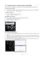
4.1. Filter
It is a common practice to remove molecules localized with poor precision, or with unrealistic
parameters. The filtering criteria can be formulated in the Filter text field as an expression
combining mathematical and logical functions and operators with parameters from the table of results
obtained from previous data analysis.
The syntax and semantics rules for the formula interpreter are similar to the ones used in the threshold
selection described in Section 6. The variables are scalars and vectors, where vectors are columns in
the table of results specified by their names without units, e.g., id, frame, x, y, sigma, intensity,
offset, bkgstd, uncertainty. The result of the formula must be a vector of booleans (true or false)
for every molecule in the table. Only molecules with the condition equal to true are accepted. Built-in
functions are the same as in Section 6, plus there are two logical functions “a & b” (AND) and
“a | b” (OR).
Examples of filter expressions
·
·
·
·
sigma>15
frame<1000 | frame>2000
intensity>100 & uncertainty<20
(x-10000)^2+(y-10000)^2<2000^2
Example of creating a filter expression using a histogram
Bad fits causing grid artefacts
Super-resolution image with grid artefacts
Filtered super-resolution image
2
3
1
10
1) Select Plot histogram and select the parameter of choice (e.g., sigma).
2) Draw a rectangular selection in the histogram specifying the minimum and the maximum accepted
value and press Apply ROI to filter. This inserts the formula into the Filter text field
automatically.
3) Press Apply to apply the filtering rule and to update the image preview.
4.2. Remove duplicates
Repeated localizations of single molecules in one frame may occur due to overlapping fitting subregions when using multiple-emitter analysis approach. ThunderSTORM allows users to specify
a radius below which molecules in close proximity are grouped together. Only the molecule with the
smallest localization uncertainty in the group is kept, other molecules are removed. The radius can be
specified as a mathematical expression which yields a scalar (same radius for all molecules, e.g.,
5*mean(uncertainty)) or a vector (different radius for every molecule, e.g., 3*uncertainty).
4.3. Merging
A single photo-activated molecule may appear in several sequential images. Such molecules can be
combined into one single molecule based on a user-specified distance. After merging, a new column
called detections appears in the table of results, showing the number of merged molecules. This new
column can also be used for filtering.
Right-click on a particular row in the table
of results and select Show list of
merged molecules to see the list of
molecules merged in that row.
4.4. Drift correction
ThunderSTORM supports lateral drift correction using the cross-correlation method.
Plot of lateral drift in time.
Cross-correlation image.
11
4.5. Z-stage offset
The axial field of view in 3D experiments can be extended by acquiring the data in multiple Z-stage
positions. This method corrects the absolute axial positions of each molecule.
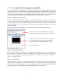
4.6. Visualizing and exporting molecular localizations from a region of interest
1)
2)
3)
4)
5)
6)
7)
8)
Select a rectangular region of interest (ROI) in the live preview image.
Press Restrict to ROI. A logical expression defining the ROI will be included in the Filter.
To resize the preview, or to visualize the data in the selected region, press Visualization.
Press Auto size by results to define the image coordinates based on ROI.
Set the visualization method and the desired magnification.
Press Use for preview to crop the live preview image based on ROI.
Or, press OK to visualize the final super-resolution image from the selected ROI.
To export data from the ROI, press Export.
6
1
4
2
3
5
8
6
12
7
5.
Analyzing super-resolution images with ImageJ
Here we provide few examples of how ImageJ can be used for analyzing super-resolution images.
Setting image properties
1)
The first step is to set the units and pixel size in the super-resolution image using the command:
Image → Properties ... (Ctrl+Shift+P)
Drawing a scale bar
1)
A scale bar can be drawn using command:
Analyze → Tools → Scale Bar ...
Measuring size of objects
1)
2)
Draw a region, e.g., free hand selection, around object of interest.
Measure the object size using command:
Analyze → Measure (Ctrl+M)
Measuring an intensity profile
1)
2)
3)
Line selection: set line width (double click on the line tool) and draw a line across the object of
interest.
Rectangular selection: A rectangular selection can be used only for horizontal intensity profiles.
Therefore, the image might need to be rotated first so that the structure of interest is vertical using
command: Image → Transform → Rotate ...
The intensity profile can be plotted using the command Analyze → Plot Profile (Ctrl+K).
13
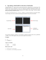
6.
Specifying a threshold for detection of molecules
ThunderSTORM uses a single-valued intensity threshold which is updated for every input image. The
threshold value can be specified by users as an expression combining mathematical functions and
operators with variables based on the current raw or filtered image. This is a powerful option, because
users can specify the threshold value systematically for unknown input images, where the global
intensity may slowly fluctuate over time.
Use the Preview button in the Run analysis window to see which molecules are detected with the
current settings. This can be useful for fine-tuning the threshold value given by the formula.
Original image
Filtered image
Calculated
threshold value
Detections
The formula interpreter provides several built-in statistical functions and some predefined
variables. A brief description of the syntax and semantic rules follows.
Examples
·
·
·
150
3*std(Wave.F1)
0.2+min(F)
Types of variables
·
·
Scalar
Matrix
– a number
– an image
Main syntax rules
·
·
all names are case insensitive
use a period (.) as a decimal point delimiter
14
Built-in operators
·
·
·
·
·
·
a
a
a
a
a
a
+
–
*
/
%
^
b
b
b
b
b
b
–
–
–
–
–
–
addition
subtraction
multiplication
division
modulo
b-th power of a
Semantics (all matrix operations are performed element-wise; matrices must have the same size)
·
·
·
scalar + scalar = scalar
matrix + matrix = matrix
matrix + scalar = matrix (scalar is added to each element of the matrix)
Built-in functions
·
·
·
·
·
·
·
·
var(x)
std(x)
mean(x)
median(x)
min(x)
max(x)
sum(x)
abs(x)
–
–
–
–
–
–
–
–
variance of x
standard deviation of x
mean value of x
median of x
minimum in x
maximum in x
sum of all items in x
absolute value of x
Variables provided by different feature enhancement filters
All the filters provide these variables:
·
·
I
F
– input image without any changes
– final filtered image
Variables representing the filters:
·
·
·
·
·
·
·
–
Med.F
–
Gauss.F
–
LowGauss
–
DoG.F
–
o DoG.G1 –
o DoG.G2 –
DoB.F
–
o DoB.B1 –
o DoB B2 –
Wave.F
–
o Wave.F1 –
o Wave.F2 –
o Wave.F3 –
Box.F
Averaging (Box) filter
Median filter
Gaussian filter
Lowered Gaussian filter
Difference-of-Gaussians filter
Input image filtered by 1st Gaussian function of DoG filter
Input image filtered by 2nd Gaussian function of DoG filter
Difference of averaging filters
Input image filtered by 1st Box of DoB filter
Input image filtered by 2nd Box of DoB filter
Wavelet filter
1st Wavelet level of the input image
2nd Wavelet level of the input image
3rd Wavelet level of the input image
15
7.
Generator of simulated data
ThunderSTORM is capable of generating a sequence of SMLM-like images in which the ground-truth
positions of the molecules are known. Users can specify the image size, sequence length, and ranges
for the intensity, imaged size, and spatial density of the generated molecules. The spatial density of the
molecules can be varied according to a user-supplied grayscale image.
Plugins → ThunderSTORM → Performance testing → Generator of simulated data
Camera parameters setup.
Size of the generated image stack.
Parameters of the generated molecules and
background noise.
Simulated sample drift in the lateral dimension.
Grayscale image used to vary the spatial density
of molecules. Note that the size can be different
from the size of the image stack.
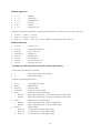
8.
Performance evaluation
If ground truth molecular positions are available, ThunderSTORM can evaluate the performance of the
processing methods. Ground truth data can be created by the generator of simulated data described in
Section 7, or imported from a file by selecting Plugins → ThunderSTORM → Import/Export →
Import ground-truth. To start evaluation, select Plugins → ThunderSTORM → Performance
testing → Performance evaluation, enter the tolerance radius for accepting true-positive
detections, and click OK. The results indicate true-positive detections (green), false positive detections
(red), false negatives (orange), and related statistical measures (e.g., recall, precision, F1 score).
16
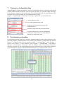
9.
Monte Carlo simulations – an example using the ImageJ
Macro Language
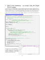
Any procedure in ThunderSTORM can be automated using the ImageJ Macro Language. Here we
show an example of a Monte-Carlo simulation which searches for an optimal threshold value for
different configurations of various localization algorithms. This example can be easily extended to any
other combination of functions, such as automated sequential processing of several different datasets.
To get more information about the ImageJ Macro Language, see the official documentation at
http://rsb.info.nih.gov/ij/developer/macro/macros.html.
requires("1.46c");
// because of `Array.concat` and `Array.slice` functions
run("Generator of simulated data", "width=256 height=256 frames=1000 density=0.3 "+
"addpoissonvar=30.0 fwhmrange=200:350 intensityrange=700:900 driftdist=0.0 "+
"driftangle=0.0");
filters = newArray("[Lowered Gaussian filter] sigma=1.6 size=11",
"[Difference-of-Gaussians filter] sigma1=1.3 sigma2=1.8 size=11",
"[Wavelet filter] level=[use 2nd wavelet level]");
colors = newArray("red","blue","magenta");
labelX = newArray(0.05, 0.33, 0.7);
labelText = newArray("Lowered Gaussian","Difference Of Gaussians","Wavelet");
xvals = newArray();
yvals = newArray();
len = 9;
fmax = 3;
for(f = 0; f < fmax; f += 1) {
run("Clear Results");
for(thr = 1.0, r = 0; thr <= 5.0; thr += 0.5, r += 1) {
selectWindow("ThunderSTORM: artificial dataset");
run("Run analysis", "filter="+filters[f]+
" detector=[Local maximum] connectivity=8-neighbourhood threshold="+thr+
"*std(F) estimator=[PSF: Integrated Gaussian] sigma=1.6 "+
"method=[Least squares] fitradius=3 mfaenabled=false renderer=[No Renderer]");
run("Performance evaluation","tolerance=50");
setResult("Threshold multiplier",r,thr);
xvals = Array.concat(xvals, thr);
yvals = Array.concat(yvals,getResult("F1-measure",r));
}
}
Plot.create("Simulation results", "threshold multiplier", "F1-measure");
Plot.setLimits(1.0,5.0,0.0,1.0);
for(f = 0; f < fmax; f += 1) {
x = Array.slice(xvals,f*len,(f+1)*len);
y = Array.slice(yvals,f*len,(f+1)*len);
Plot.setColor(colors[f]);
Plot.add("line",x,y);
Plot.add("x",x,y);
Plot.addText(labelText[f], labelX[f], 0.1);
}
Plot.show();
Note that results of the simulation can
be further improved by using a more
complex threshold for approximate
molecular localizations, or by more
complex post-processing rules.
17